Image sensing with multilayer, nonlinear optical neural networks

Tianyu Wang These authors contributed equally. School of Applied and Engineering Physics, Cornell University, Ithaca, NY 14853, USA Mandar M. Sohoni These authors contributed equally. School of Applied and Engineering Physics, Cornell University, Ithaca, NY 14853, USA Logan G. Wright School of Applied and Engineering Physics, Cornell University, Ithaca, NY 14853, USA NTT Physics and Informatics Laboratories, NTT Research, Inc., Sunnyvale, CA 94085, USA Martin M. Stein School of Applied and Engineering Physics, Cornell University, Ithaca, NY 14853, USA Shi-Yuan Ma School of Applied and Engineering Physics, Cornell University, Ithaca, NY 14853, USA Tatsuhiro Onodera School of Applied and Engineering Physics, Cornell University, Ithaca, NY 14853, USA NTT Physics and Informatics Laboratories, NTT Research, Inc., Sunnyvale, CA 94085, USA Maxwell Anderson School of Applied and Engineering Physics, Cornell University, Ithaca, NY 14853, USA Peter L. McMahon To whom correspondence should be addressed:
tw329@cornell.edu, mms477@cornell.edu, lgw32@cornell.edu, pmcmahon@cornell.edu School of Applied and Engineering Physics, Cornell University, Ithaca, NY 14853, USA Kavli Institute at Cornell for Nanoscale Science, Cornell University, Ithaca, NY 14853, USA

Abstract

Optical imaging is commonly used for both scientific and technological applications across industry and academia. In image sensing, a measurement, such as of an object’s position or contour, is performed by computational analysis of a digitized image. An emerging image-sensing paradigm [1, 2, 3, 4, 5, 6] breaks this delineation between data collection and analysis by designing optical components to perform not imaging, but encoding. By optically encoding images into a compressed, low-dimensional latent space suitable for efficient computational post-analysis, these image sensors can operate with fewer pixels and fewer photons, allowing higher-throughput, lower-latency operation. Optical neural networks (ONNs), primarily developed as accelerators for deep-neural-network inference, offer a platform for processing data in the analog, optical domain [7, 8, 9, 10, 11, 4, 12, 13, 14, 15, 16, 17, 18, 19, 20]. ONN-based sensors have however been limited to linear processing, which is equivalent to a single-layer neural network (NN) [21, 22, 1, 23, 2, 24, 3, 4, 25, 26, 27, 28, 29, 30]. Nonlinearity is a prerequisite for depth, and multilayer NNs significantly outperform shallow NNs on many tasks, including image processing and compression [31, 32, 33]. Here, we realize a multilayer ONN pre-processor for image sensing, using a commercial image intensifier as a parallel optoelectronic, optical-to-optical nonlinear activation function. We demonstrate that the nonlinear ONN pre-processor can achieve compression ratios of up to 800:1 – corresponding to compressing the input to just a two-dimensional output vector – while still enabling high accuracy across several representative computer-vision tasks, including machine-vision benchmarks, flow-cytometry image classification, and measurement and identification of objects in real scenes. In all cases we find that the ONN’s nonlinearity and depth allowed it to outperform a purely linear ONN encoder. Although our experimental demonstrations are specialized to ONN sensors for incoherent-light images, the growing multitude of ONN platforms should facilitate a range of ONN sensors. These ONN sensors may surpass conventional sensors by pre-processing optical information in spatial, temporal, and/or spectral dimensions, potentially with coherent and quantum qualities, all natively in the optical domain.

I Introduction

Optical images are widely used to capture and convey information about the state or dynamics of physical systems, both in fundamental science and in technology. They are used to guide autonomous machines, to assess manufacturing processes, and to inform medical diagnoses and procedures. In all these applications, an optical system such as a microscope forms an image of a subject on a camera, which converts the photonic, analog image into an electronic, digital image. Digital images are typically many megabytes. For most applications however, nearly all this information is redundant or irrelevant. There are three main reasons: (i) natural images contain sparse information, and are therefore compressible [1, 34, 35]; (ii) most applications involve images of subjects with additional underlying commonalities beyond sparsity, and (iii) most information in an image is irrelevant to the image’s end use. Here, we refer to machine-vision applications, for which factor (iii) is applicable, as image sensing – for these applications only a specific subset of information from each image is sought, as depicted in Figure 1a.

The information inefficiency of conventional imaging has inspired machine-vision paradigms in which optics are designed not as a conventional imaging system, but instead as an optical encoder – a computational pre-processor that extracts relevant information from an image [1, 2, 3, 4, 25, 26, 6, 27, 28, 29, 30]. Techniques include end-to-end optimization [21, 22, 23, 36, 24, 3, 26, 37, 6, 38, 39, 27, 29, 30], compressed sensing and single-pixel imaging [1, 40, 35, 41], coded apertures [42, 39, 43, 28, 30], and related approaches for computational lensless imaging [44, 45]. A common feature and limitation of these techniques is that the optics perform only linear operations. In end-to-end optimization, where the processing algorithm is usually a DNN, the optical system is effectively a linear encoder equivalent to a single-layer NN [24, 3, 26, 4, 27, 28]. Since these approaches may emulate the hierarchical information distillation of biological vision, some are considered neuromorphic [46, 34, 47]. Related trends include the broader fields of smart cameras [5], in- and near-sensor computing [48, 49, 25], variational quantum sensors [50], and machine-learning-enabled smart sensors [51, 52].

Optical pre-processing allows image-sensing systems to overcome a fundamental bottleneck in performance, enabling faster, smaller, and more energy-efficient image sensors. In a conventional image sensor, using a camera with $C$ -fold fewer pixels typically leads to a $C$ -fold improvement in achievable frame rate, number of photons per pixel, system power, size, weight, and cost, and at least a $C$ -fold-lower decision latency. The reason for this is that these performance metrics are directly bottlenecked by the speed and energy cost of transducing images from the optical to digital electronic domain, of transporting them from the sensor to post-processor, and of post-processing high-dimensional digital image data. Nevertheless, conventional imaging pixel resolution cannot be reduced significantly without losing important content. This fundamental trade-off can be circumvented by using optical encoders to compress images into a low-dimensional latent feature space. In most applications, compression by $\gg$ 10 times is in principle feasible. However, while such high compression is routinely achieved with electronic DNNs, the computational capacity of simple optical encoders (such as single random or optimized masks) is rarely sufficient.

Fortuitously, more computationally capable optical encoders are now within reach due to recent advances in optical neural networks (ONNs) [4, 15, 19]. ONNs are optoelectronic systems that optically perform mathematical operations involved in typical DNN inference calculations. By taking advantage of the large number of optical modes available in space, time, or frequency [53, 4], ONNs allow completely parallel, optical-domain computation of wide and densely connected layers in DNNs [10, 11, 4, 16], with the potential be orders of magnitude faster than electronic DNNs [13, 15, 19]. While most experimentally demonstrated ONNs have involved only linear operations, such as matrix-vector multiplications and convolutions, being performed optically, it is widely appreciated that ONNs should also incorporate nonlinear activation functions [4]. Compelling proposals for and early demonstrations of this have been reported [54, 55, 56, 57, 58], but the problem of developing a suitable nonlinearity that can enable large-scale, deep ONNs is still considered a major outstanding challenge in the field [4].

ONNs are thus ideal for enabling a new class of image sensing devices, ONN sensors [59, 2, 3, 4, 26, 25, 19, 27], in which an ONN pre-processes data from and in the analog optical domain, prior to its conversion into digital-electronic signals. While linear ONNs still expand the capabilities of end-to-end-optimized image sensors compared to simpler optical systems, the pre-processing they provide is nonetheless still mathematically equivalent to at most a single NN layer. Depth -– and nonlinearity –- are essential for high-performance, efficient NN image processing: deep, nonlinear networks are exponentially (in the number of neurons) more efficient than single-layer NNs at approximating practically relevant functions [60, 61].

Here, we demonstrate an optical neural network image sensor that uses an optoelectronic optical-to-optical nonlinear activation (OONA) to perform multilayer ONN pre-processing for a variety of image sensing applications. Our multilayer, nonlinear ONN pre-processor conditionally compresses image data into a low-dimensional latent feature space in a single shot, achieving compression ratios up to 800:1. At high compression ratios, our device consistently outperforms conventional image sensing and linear optical pre-processing on experiments based on standard machine vision datasets, on flow cytometry image classification, and for real-scene object detection and measurement. The OONA used in our experiments is based on a commercial image intensifier typically used, e.g., in night-vision goggles or low-light scientific imaging. The linear layers (matrix-vector multiplications) in our ONN are implemented using a technique designed to facilitate incoherent images as direct inputs, with a microlens array for all-optical fan-out. Broadly, our findings support the use of multilayer ONNs with nonlinear activations as optical-domain pre-processors for sensors. Given the numerous ONN platforms and optical nonlinear activations now being developed, we expect that a multitude of deep ONN sensors is possible; these future sensors may detect information encoded in light’s spatial, spectral, and/or temporal degrees of freedom.

II An ONN-based image sensor with optical-to-optical nonlinearity

Refer to caption — Figure 1: A multilayer optical-neural-network encoder as a frontend for image sensing. a, Image sensing via direct imaging vs optical encoding. In conventional image sensing, an image is collected by a camera, and processed, often using a neural network (NN), to extract a small piece of relevant information, such as the speed limit or text of a sign. Rather than faithfully reproducing the full image of a scene onto the sensor array, an optical-neural-network (ONN) encoder instead pre-processes the image, compressing and extracting only the image information necessary for its end use, allowing a much smaller (fewer pixel) sensor array. b, The neural-network diagram and corresponding mathematical operations of the ONN encoder used in this study. The ONN encoder consists of interleaved linear and nonlinear layers before the compressed signal is captured by a small photodetector array. $\vec{x}$ : input image; $W_{i}$ : weight matrix of fully connected layer $i$ ; $\sigma$ : optical-to-optical nonlinear activation function; $f_{\text{digi}}$ : digital backend function. c, The schematic of the fully optical matrix-vector multiplier used for constructing both linear layers in (b). d, The schematic of the optical-to-optical nonlinear activation layer realized with a saturating image intensifier. The inset plot shows that the output light intensity of a single spatial mode begins to saturate as the input light intensity increases, resembling the sigmoid activation function.

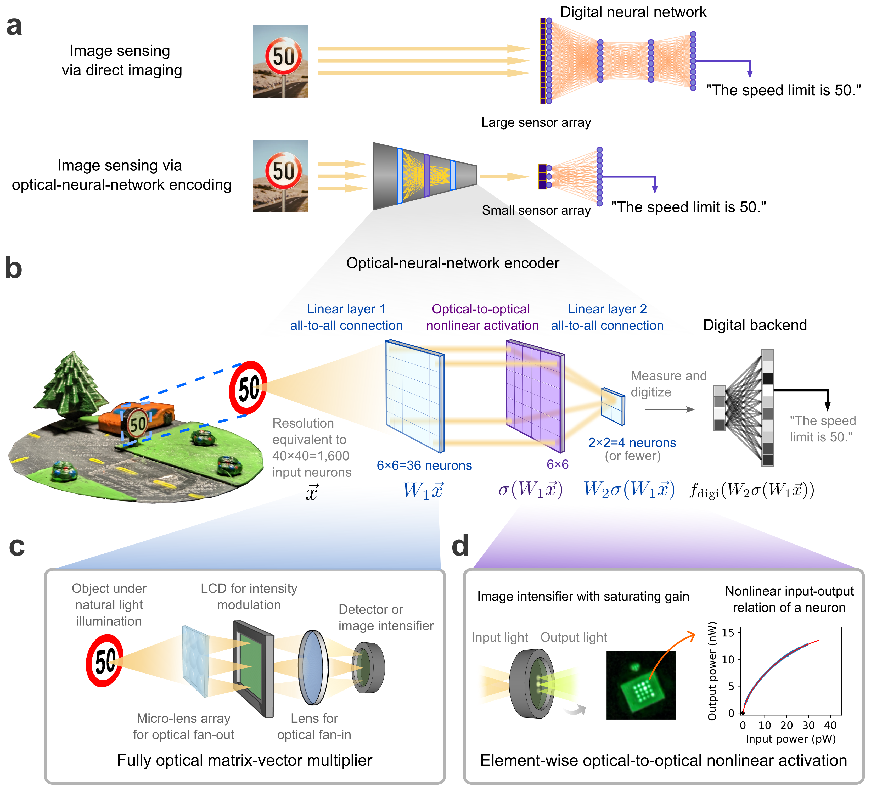
Our experimental optical-neural-network (ONN)-based image sensor consists of a 2-layer, fully connected optical neural network in which the optical-to-optical, element-wise nonlinear activation function following the first layer is realized by a saturating microchannel plate inside a commercial image intensifier. The sensor read-out is implemented by a CMOS camera and subsequent digital post-processing. The optical pre-processor implements a nonlinear encoder – it maps input images carried by incoherent light to an abstract, lower-dimensional latent space. In our work, the encoder is not intended to perform lossless image compression. Instead, the optical encoder is trained to preserve only the information most relevant to a given image-sensing task (Fig. 1a).

Imaging applications typically involve broadband, incoherent ambient light, so our device was designed to operate directly on broadband, incoherent visible light images. Starting with fanout – which effectively creates copies of the input image – implemented by an array of microlenses, optical fully connected matrix-vector multiplications are performed using a method similar to previous works [16, 17, 29] (see Methods and Supplementary Note 2). Briefly, multiplication is achieved by attenuating the copies of the input image in proportion to the components of the weight matrix, and the summation of each output vector element is realized by focusing the attenuated light components using a lens (Fig. 1d). To realize the optical-to-optical nonlinear activation (OONA) operations applied to each element of this output vector, light is focused onto an image intensifier tube. Incident light generates free electrons from a photocathode, which are locally amplified by a microchannel plate (MCP) and then produce new, amplified bright spots as they strike a phosphor screen [62]. The local saturation of the MCP’s amplification leads to a saturating nonlinear response, qualitatively similar to the positive half of the sigmoid function (Fig. 1e and Supplementary Figure 8). Although the OONA is optoelectronic, rather than all-optical, its local, in-place realization preserves the spatial parallelism of the ONN, and avoids the time and energy costs required for read-out/in when the nonlinear activation is computed on a separate electronic processor, as in some previous work [59, 16, 17]. To implement the second layer of the ONN, the light produced by the intensifier is processed by a second copy of the optical matrix-vector multiplier depicted in Figure 1d. The output from this layer is detected by up to 4 binned superpixels of a camera (see Methods), but in principle can be captured by an array of 4 photodetectors.

To compare the multilayer, nonlinear ONN encoder to conventional (direct) image sensing and to a single-layer, linear ONN encoder, we included a beamsplitter prior to the intensifier OONA, which allowed us to reconfigure the image sensor for direct imaging (by setting the LCD from the first linear layer to be transparent) and for single-layer ONN pre-processing (by applying linear-layer weights to the first LCD).

II.1 Nonlinear ONN encoders extract information more effectively than linear encoders

Figure 2: Comparison between linear ONN and nonlinear ONN encoders on diverse image classification tasks. a, Classification of hand-drawn figures from 10 different classes in the Quick, Draw! (QuickDraw) dataset. b, The results of QuickDraw [63] classification with a linear or, c, nonlinear ONN encoder as the frontend. The neural-network architecture with corresponding mathematical operations is placed above the confusion matrix it produces (blue slabs: layers of linear optical neurons, purple slabs: layers of nonlinear activation function, grey bars: layers of digital neurons.

\vec{x}

: input image;

W_{i}

: weight matrix of fully connected layer

i

;

\sigma

: optical-to-optical nonlinear activation function). d, Comparison of the accuracy derived from classifiers equipped with different frontends, including direct imaging (with downsampling), a linear ONN encoder, a linear digital electronic encoder, a nonlinear ONN encoder, and a nonlinear digital electronic encoder (from left to right). In all cases, the encoder’s output dimension (number of pixels) is 4. e, Classification of HeLa cells labeled for different organelles from a dataset acquired from flow cytometry experiments [64]. f, The results of cell-organelle classification with a linear, or a nonlinear g ONN encoder as the frontend. The neural-network architecture is placed above the confusion matrix it resulted in. h, Visualization of the compressed cell-organelle data with density uniform manifold approximation and projection (DensMAP) [65]. The data points are labeled as the ground truth. i, Recognizing 3D objects: each of 8 3D-printed speed-limit signs are viewed from different perspectives by an optical encoder, to classify the speed-limit number on the sign. j, The results of classifying speed limits with a linear or, k, a nonlinear ONN encoder as the frontend. The neural-network architecture is shown above the confusion matrix it produces. l, Classification accuracy as a function of the viewing angle. The shaded area denotes one standard deviation from the mean for repeated classification tests.

To evaluate the performance of the multilayer, nonlinear ONN encoder, we first performed several image classification tasks, summarized in Figure 2. As a benchmark, we trained classifiers for 10 pre-selected classes of the Quick, Draw! (QuickDraw) image dataset [63]. Input images (28×28 pixels) were binarized and displayed on a digital micromirror display (DMD), which was placed in front of each image sensor (nonlinear multilayer, linear single-layer, and direct imaging). For a direct comparison, the vector dimension at the optical-electronic bottleneck in each sensor is the same, a 2×2 array or 4-dimensional latent space, which represents a 196:1 image-compression ratio. The nonlinear, multilayer ONN sensor achieves better classification accuracy than the other sensors (Fig. 2b-c). Since our ONN components are not perfectly calibrated, they typically perform slightly worse than digital neural networks with similar architectures. To ensure that the accuracy advantage of the nonlinear, multilayer ONN encoder is consistently better than any possible linear encoder with the same bottleneck dimension, we also trained all-digital (with real-number weights and biases) single-layer linear encoders for the same task, without image downsampling (Fig. 2d). Despite the constraint of non-negative weights and the non-analytical form of our OONA, the experimental, multilayer nonlinear ONN encoder’s performance (79% test accuracy) robustly surpasses that of linear encoders, beating both the optical (69.5%) and optimized digital (74%) single-layer encoders. Compared to an ideal digital multilayer encoder with real-valued weights plus biases and sigmoid nonlinear function, the experimental nonlinear ONN encoder has a reduced test accuracy but not by much (79% vs 82%).

To explore the potential of ONN image sensors for a more practically important application, we next tested our image sensors on the task of classifying fluorescent images of cell organelles acquired in a flow-cytometry device [64]. Image-based flow cytometry is an emerging technique in which cells are pulled through a microfluidic tube and imaged, ideally one-by-one, e.g., by fluorescence and/or phase imaging [66, 67, 68, 64]. The cells can be autonomously sorted if each image can be analyzed quickly to determine the type of cell or the cell’s characteristics. In order to process statistically useful collections of cells, so as to detect, e.g., extremely rare cancerous cells, it is essential to minimize the latency of each sorting decision to maintain a high throughput, such as 100,000 cells per second [67, 68, 64]. In our experiments, we displayed binarized images from the dataset in Ref. [64] on the DMD and performed classification with each sensor, as in the QuickDraw experiments (Fig. 2e). The multilayer, nonlinear ONN encoder compresses the input images by an effective ratio of 400:1, and results in a classification accuracy for the 5 considered classes that is better than the linear-ONN sensor (93% vs 88.5% test accuracy, Fig. 2f and g; higher local density within clusters, Fig. 2h).

The two tasks considered so far are effectively experimental simulations of image-sensing tasks; real image-sensing tasks involve directly processing photons arriving from real 3D objects. To test this setting, we applied the image sensors to the task of classifying traffic signs in a real-model scene, the 3D-printed intersection shown in Fig. 2i. Due to the limited field-of-view of the particular microlens array used in this experiment, the input images to the image sensors (insets of Fig. 2g) contain primarily only the speed limit sign being classified. The nonlinear, multilayer ONN encoder results in better identification of the speed limit than the linear ONN encoder across a range of viewing angles from 0 to 80 degrees (Fig. 2j-l).

II.2 The same optically compressed features enable a variety of image-sensing applications

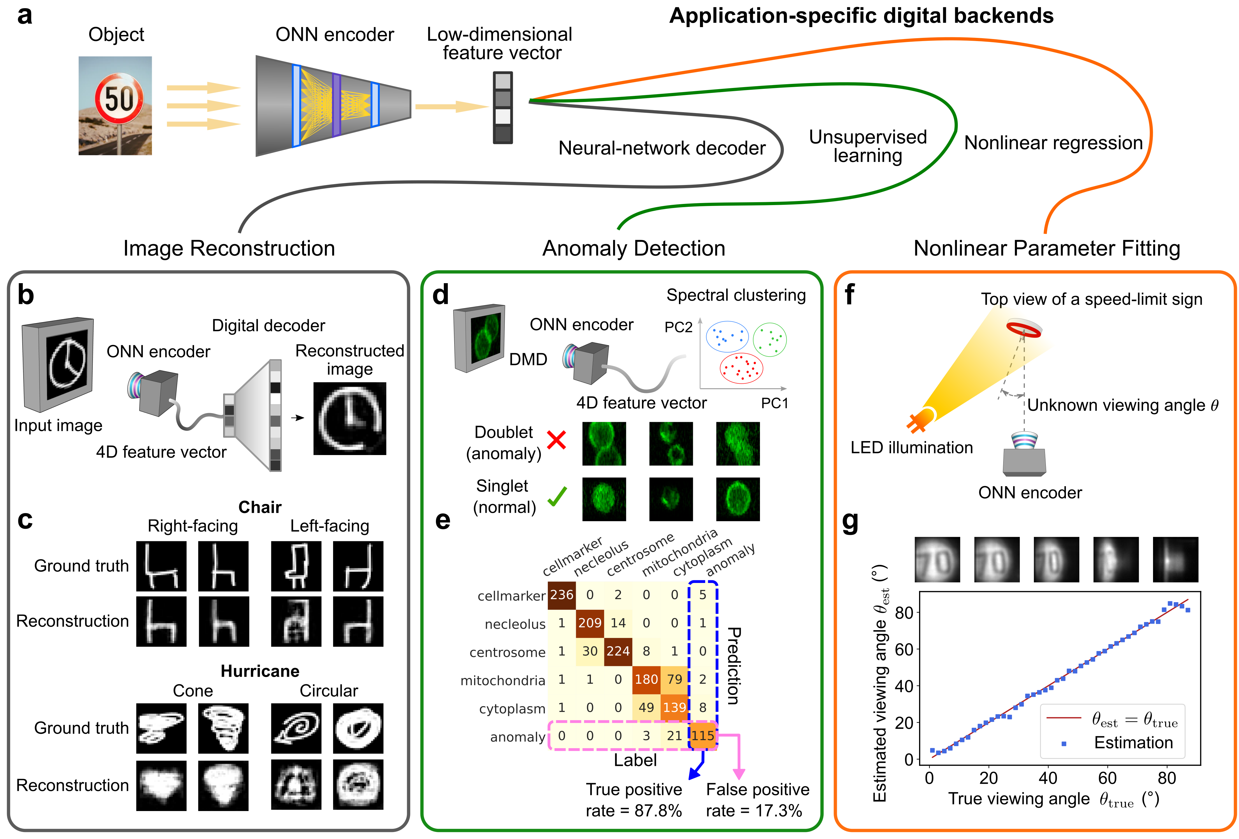
By training new digital post-processers only, the same optical encoders trained for classification in the previous section can be re-used for a variety of other image-sensing tasks. If suitably trained (see Methods), encoders can produce robust representations of high-dimensional images in the low-dimensional latent space, which preserve far more information than the bare minimum required for classification. For example, although the QuickDraw-classification encoder (Fig. 2a-c) was trained only to facilitate classification, the feature space evidently preserves more complex attributes of the original images beyond just the figure’s class. When a digital decoder is trained to reconstruct QuickDraw images from the classification encoder’s features (Fig. 3b-c), it produces reconstructions that, while often lacking specific details (like the position of the clock’s hands), captures coarse intra-class details like the orientation or shape of chairs and hurricanes.

Similarly, using the same multilayer ONN encoder previously trained for traffic-sign classification (Fig. 2i-l), we trained a new digital backend to predict the angle at which a traffic sign was viewed (Fig. 3f and 3g). The resulting predictions are very accurate, although the performance is reduced if the network is required to predict viewing angle for all, rather than just one, speed-limit class at a time (Supplementary Figure 24).

Finally, in many image-sensing applications, initial device training will not be able to account for edge cases that may be encountered in deployment. To test the capacity for anomalies not previously observed (and on which the optical encoder was not trained) to be detected, we introduced anomalous images of doublet cell clusters to the ONN image sensor (Fig. 3d). To detect these anomalies, we applied spectral clustering to the normalized 4-dimensional feature vectors produced by the ONN encoder previously trained for cell-organelle classification (see Methods). By identifying the six most prominent clusters as the five trained classes, plus one class corresponding to anomalous images, we were able to adapt the digital decoder to reliably identify anomalous images in the test set (Fig. 3e). These results show that the nonlinear ONN encoder does not overfit to the initial training dataset, but instead preserves important data structure beyond the initially chosen classes, while still compressing the original images to a low-dimensional space.

III Multilayer ONN sensors scale favorably to complex image sensing tasks

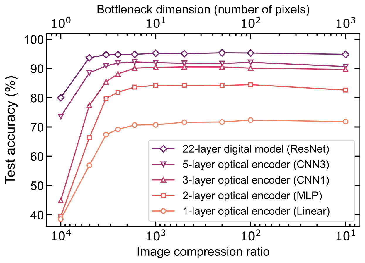
The results presented in Figs 2 and 3 illustrate that a 2-layer nonlinear ONN pre-processor enables consistently better image-sensing performance than conventional imaging with direct downsampling or linear-ONN pre-processing, across a wide range of tasks. Nonetheless, ONN encoders with two fully connected layers is merely a first step. A key motivation for using an OONA is that it will facilitate even deeper ONN encoders and, in turn, facilitate more sophisticated optical pre-processing. To explore what may soon be possible with deeper, nonlinear ONN encoders, we performed realistic simulations of four different optical pre-processors, each with a different number of nonlinear and linear optical layers (see Figure 4), performing an extended (10-class) version of the organelle-classification task considered in Figs 2-3 (Supplementary Figure 25). We chose this dataset, which is more challenging than the 5-class cell-organelle classification demonstrated in earlier experiments, so that we could study the performance for more complicated ONN encoders. Our simulations (see Methods for details) consider physical noise, and involve strictly non-negative weights, which is a critical constraint for ONNs operating on incoherent light, such as fluorescence.

Figure 4 shows how the classification accuracy of the different ONN pre-processors varies as the compression ratio is changed. The compression ratio is changed by modifying the number of output neurons in the final optical layer, which determines the number of pixels or photodetectors required on the photosensor. As a reference for achievable performance, we also performed the task with a fully digital classifier based on a ResNet model (18-layer pretrained ResNet plus 4 additional adapting layers) [69]. All networks, including the all-digital reference, have the same single-layer digital decoder architecture.

The key result in Fig. 4 is that deeper ONNs, incorporating multiple nonlinear layers, lead to progressively better classification performance across a wide range of compression ratios. The benefit of pre-processor depth becomes especially evident at very high compression ratios: for a compression ratio of $10^{4}$ (bottleneck dimension 1) the 5-layer pre-processor (CNN3) achieves nearly double the accuracy of shallower networks.

IV Discussion

Our results show that nonlinear, multilayer optical neural network (ONN) image pre-processors enable image sensors that outperform both image sensors based on conventional direct imaging, and those with only linear-optical pre-processing at high-compression ratios. In this high-compression regime, through a diverse range of image-sensing tasks, we show that deep, nonlinear optical image pre-processing enables better extraction of image information, resulting in better image-sensing performance. Furthermore, we see that the performance advantages of nonlinear ONN encoders scale favorably with additional layers of ONN pre-processing. Such nonlinear optical encoders extend the paradigm of end-to-end image system optimization [21, 22, 23, 36, 24, 3, 37, 26, 39, 38, 27, 29, 30] to include more powerful nonlinear optical image pre-processing. As their capabilities are improved, we anticipate nonlinear ONN sensors will provide versatile, almost universal frontends for processing images in the analog, optical domain, facilitating both quantitative and qualitative advances throughout image sensing and machine vision.

Although the performance advantages possible with ONN-based optical frontends might appear to come at the cost of increasing overall device complexity, the opposite may turn out to be true. In traditional optical sensors, the optical system must be optimized to agnostically preserve as much information in the incident optical signal as possible, since any of the image’s content could in principle be relevant to the end use. In an ONN-based sensor, the amount of information that must be preserved can be far less (only the relevant information), and distortions (including many manufacturing imperfections) may simply be adapted to by parameter adjustments, enabling, in principle, smaller, cheaper, and easier-to-manufacture optoelectronic systems for image sensing.

Perhaps the most compelling evidence supporting the potential future impact of ONN-based sensors is the wide-ranging, rapid modern development of relevant optoelectronic technology. While ONNs, and even ONN-based sensors, were considered three decades ago (e.g., Refs [7, 54, 70, 59]), bringing these inspiring concepts beyond the laboratory is only recently starting to become feasible [9, 4]. This is in part due to advances in relevant optoelectronics and nanophotonics needed to create low-cost, mass-manufacturable and small-footprint realizations of ONN devices, such as 2D-material optoelectronics [25, 71, 52], optical metasurfaces [72, 73, 74, 27], large-scale VCSEL arrays [75, 76], as well as silicon nanophotonics and micro-optoelectronics. Additionally, a key driver for this technology today is the anticipated demand for optical deep learning accelerator hardware [9, 4]. This application, motivated by the surging computation demands required for scaling deep-neural-network models, has inspired ONN hardware platforms that process information encoded not just in optical spatial modes, but also in time, frequency or mixed domains [10, 11, 4, 12, 15, 13, 14].

The diversity of emerging ONN platforms suggests a multitude of ONN sensors will soon be possible to realize. ONN processors that process information encoded in different spatial degrees-of-freedom could be used to adapt the image-sensing paradigm to other optical degrees-of-freedom, extracting information not from incoherent-light images but rather from optical spectroscopic traces, or hyperspectral, LiDAR, or coherent image inputs. For high-resolution image sensing, a free-space-facing ONN platform will still be necessary for early network layers, but integrated, compact ONN platforms could be used to partially or entirely replace the digital backend used in our work, taking as inputs directly the low-dimensional optical outputs of the free-space-facing layers. By entirely bypassing electronic bottlenecks on speed, sensitivity, and resolution, these all-optical intelligent sensors could one day operate with multi-THz bandwidth, gigapixel effective spatial resolution, and picosecond-scale latency.

Data and code availability

Demonstration code for data gathering, and the code for training for all optical/digital neural networks is available at: https://github.com/mcmahon-lab/Image-sensing-with-multilayer-nonlinear-optical-neural-networks. All data generated and code used in this work is available at: https://doi.org/10.5281/zenodo.6888985.

Acknowledgements

The authors wish to thank NTT Research for their financial and technical support. Portions of this work were supported by the National Science Foundation (award CCF-1918549) and a David and Lucile Packard Foundation Fellowship. P.L.M. acknowledges membership of the CIFAR Quantum Information Science Program as an Azrieli Global Scholar. We acknowledge helpful discussions with Alen Senanian, Benjamin Malia, Federico Presutti, Vladimir Kremenetski, Sridhar Prabhu, Anna Barth, and Rachel Oliver. We also acknowledge Sonalee Sohoni for help with figure design.

Author Contributions

T.W., L.G.W., Mandar M.S., and P.L.M. conceived the project and designed the experiments. Mandar M.S. and T.W. built and performed the experiments on the nonlinear and linear ONN encoders, and analyzed the data. T.W. performed the extended cell-organelle simulations. Martin M.S. performed the neural architecture search for QuickDraw reconstruction. S.M. and T.O. aided in simulations of deep optical encoders. M.G.A. assisted with 3D-scene modelling. L.G.W., T.W., Mandar M.S. and P.L.M. wrote the manuscript. P.L.M. and L.G.W. supervised the project.

Competing Interests

T.W., Mandar M.S., L.G.W. and P.L.M. are listed as inventors on a U.S. provisional patent application (Serial No. 63/392,042) on nonlinear optical neural network pre-processors for imaging and image sensing.

References

[1] Duarte, M. F. et al. Single-pixel imaging via compressive sampling. IEEE Signal Processing Magazine 25, 83–91 (2008).
[2] Chang, J., Sitzmann, V., Dun, X., Heidrich, W. & Wetzstein, G. Hybrid optical-electronic convolutional neural networks with optimized diffractive optics for image classification. Scientific Reports 8, 1–10 (2018).
[3] Martel, J. N. P., Mueller, L. K., Carey, S. J., Dudek, P. & Wetzstein, G. Neural sensors: Learning pixel exposures for HDR imaging and video compressive sensing with programmable sensors. IEEE Transactions on Pattern Analysis and Machine Intelligence 42, 1642–1653 (2020).
[4] Wetzstein, G. et al. Inference in artificial intelligence with deep optics and photonics. Nature 588, 39–47 (2020).
[5] Brady, D. J. et al. Smart cameras. arXiv preprint arXiv:2002.04705 (2020).
[6] Musk, E. Tesla AI Day, https://www.youtube.com/watch?v=j0z4FweCy4M (2021).
[7] Farhat, N. H., Psaltis, D., Prata, A. & Paek, E. Optical implementation of the Hopfield model. Applied Optics 24, 1469–1475 (1985).
[8] Denz, C. Optical Neural Networks (Vieweg+Teubner Verlag Wiesbaden, 1998), 1st edn.
[9] Shen, Y. et al. Deep learning with coherent nanophotonic circuits. Nature Photonics 11, 441–446 (2017).
[10] Lin, X. et al. All-optical machine learning using diffractive deep neural networks. Science 361, 1004–1008 (2018).
[11] Hamerly, R., Bernstein, L., Sludds, A., Soljačić, M. & Englund, D. Large-scale optical neural networks based on photoelectric multiplication. Physical Review X 9, 21032 (2019).
[12] Nahmias, M. A. et al. Photonic multiply-accumulate operations for neural networks. IEEE Journal of Selected Topics in Quantum Electronics 26, 1–18 (2020).
[13] Xu, X. et al. 11 TOPS photonic convolutional accelerator for optical neural networks. Nature 589, 44–51 (2021).
[14] Feldmann, J. et al. Parallel convolutional processing using an integrated photonic tensor core. Nature 589, 52–58 (2021).
[15] Shastri, B. J. et al. Photonics for artificial intelligence and neuromorphic computing. Nature Photonics 15, 102–114 (2021).
[16] Wang, T. et al. An optical neural network using less than 1 photon per multiplication. Nature Communications 13, 1–8 (2022).
[17] Bernstein, L. et al. Single-shot optical neural network. arXiv preprint arXiv:2205.09103 (2022).
[18] Tait, A. N. Quantifying power in silicon photonic neural networks. Physical Review Applied 17, 054029 (2022).
[19] Huang, C. et al. Prospects and applications of photonic neural networks. Advances in Physics: X 7, 1981155 (2022).
[20] Sludds, A. et al. Delocalized photonic deep learning on the internet’s edge. arXiv preprint arXiv:2203.05466 (2022).
[21] Matic, R. M. & Goodman, J. W. Comparison of optical predetection processing and postdetection linear processing for partially coherent image estimation. Journal of the Optical Society of America A 6, 213–228 (1989).
[22] Kubala, K., Dowski, E. & Cathey, W. T. Reducing complexity in computational imaging systems. Optics Express 11, 2102–2108 (2003).
[23] Stork, D. G. & Robinson, M. D. Theoretical foundations for joint digital-optical analysis of electro-optical imaging systems. Applied Optics 47, B64–B75 (2008).
[24] Colburn, S., Chu, Y., Shilzerman, E. & Majumdar, A. Optical frontend for a convolutional neural network. Applied Optics 58, 3179–3186 (2019).
[25] Mennel, L. et al. Ultrafast machine vision with 2D material neural network image sensors. Nature 579, 62–66 (2020).
[26] Pad, P. et al. Efficient neural vision systems based on convolutional image acquisition. In Proceedings of the IEEE/CVF Conference on Computer Vision and Pattern Recognition, 12285–12294 (2020).
[27] Zheng, H. et al. Meta-optic accelerators for object classifiers. arXiv preprint arXiv:2201.11034 (2022).
[28] Shi, W. et al. LOEN: Lensless opto-electronic neural network empowered machine vision. Light: Science & Applications 11, 1–12 (2022).
[29] Chen, Y. et al. Photonic unsupervised learning processor for secure and high-throughput optical fiber communication. arXiv preprint arXiv:2203.03807 (2022).
[30] Bezzam, E., Vetterli, M. & Simeoni, M. Learning rich optical embeddings for privacy-preserving lensless image classification. arXiv preprint arXiv:2206.01429 (2022).
[31] Hinton, G. E. & Salakhutdinov, R. R. Reducing the dimensionality of data with neural networks. Science 313, 504–507 (2006).
[32] Krizhevsky, A., Sutskever, I. & Hinton, G. E. ImageNet classification with deep convolutional neural networks. In Proceedings of the 25th International Conference on Neural Information Processing Systems (NeurIPS) (2012).
[33] Goodfellow, I., Bengio, Y. & Courville, A. Deep Learning (MIT Press, 2016).
[34] Sterling, P. Principles of neural design (MIT Press, 2015).
[35] Gibson, G. M., Johnson, S. D. & Padgett, M. J. Single-pixel imaging 12 years on: A review. Optics Express 28, 28190–28208 (2020).
[36] Sitzmann, V. et al. End-to-end optimization of optics and image processing for achromatic extended depth of field and super-resolution imaging. ACM Transactions on Graphics (TOG) 37, 1–13 (2018).
[37] Kim, K., Konda, P. C., Cooke, C. L., Appel, R. & Horstmeyer, R. Multi-element microscope optimization by a learned sensing network with composite physical layers. Optics Letters 45, 5684–5687 (2020).
[38] Markley, E., Liu, F. L., Kellman, M., Antipa, N. & Waller, L. Physics-based learned diffuser for single-shot 3D imaging. In NeurIPS 2021 Workshop on Deep Learning and Inverse Problems (2021).
[39] Vargas, E., Martel, J. N. P., Wetzstein, G. & Arguello, H. Time-multiplexed coded aperture imaging: Learned coded aperture and pixel exposures for compressive imaging systems. In Proceedings of the IEEE/CVF International Conference on Computer Vision, 2692–2702 (2021).
[40] Liutkus, A. et al. Imaging with nature: Compressive imaging using a multiply scattering medium. Scientific Reports 4, 1–7 (2014).
[41] Li, J. et al. Spectrally encoded single-pixel machine vision using diffractive networks. Science Advances 7, eabd7690 (2021).
[42] Asif, M. S., Ayremlou, A., Sankaranarayanan, A., Veeraraghavan, A. & Baraniuk, R. G. Flatcam: Thin, lensless cameras using coded aperture and computation. IEEE Transactions on Computational Imaging 3, 384–397 (2016).
[43] Baek, S.-H. et al. Single-shot hyperspectral-depth imaging with learned diffractive optics. In Proceedings of the IEEE/CVF International Conference on Computer Vision, 2651–2660 (2021).
[44] Sinha, A., Lee, J., Li, S. & Barbastathis, G. Lensless computational imaging through deep learning. Optica 4, 1117–1125 (2017).
[45] Boominathan, V., Robinson, J. T., Waller, L. & Veeraraghavan, A. Recent advances in lensless imaging. Optica 9, 1–16 (2022).
[46] Serre, T. & Poggio, T. A neuromorphic approach to computer vision. Communications of the ACM 53, 54–61 (2010).
[47] Mead, C. How we created neuromorphic engineering. Nature Electronics 3, 434–435 (2020).
[48] Burt, P. J. Smart sensing within a pyramid vision machine. Proceedings of the IEEE 76, 1006–1015 (1988).
[49] Zhou, F. & Chai, Y. Near-sensor and in-sensor computing. Nature Electronics 3, 664–671 (2020).
[50] Marciniak, C. D. et al. Optimal metrology with programmable quantum sensors. Nature 603, 604–609 (2022).
[51] Ballard, Z., Brown, C., Madni, A. M. & Ozcan, A. Machine learning and computation-enabled intelligent sensor design. Nature Machine Intelligence 3, 556–565 (2021).
[52] Ma, C. et al. Intelligent infrared sensing enabled by tunable moiré quantum geometry. Nature 604, 266–272 (2022).
[53] Miller, D. A. B. Waves, modes, communications, and optics: A tutorial. Advances in Optics and Photonics 11, 679–825 (2019).
[54] Wagner, K. & Psaltis, D. Multilayer optical learning networks. Applied Optics 26, 5061–5076 (1987).
[55] Zuo, Y. et al. All-optical neural network with nonlinear activation functions. Optica 6, 1132–1137 (2019).
[56] Fard, M. M. P. et al. Experimental realization of arbitrary activation functions for optical neural networks. Optics Express 28, 12138–12148 (2020).
[57] Ryou, A. et al. Free-space optical neural network based on thermal atomic nonlinearity. Photonics Research 9, B128–B134 (2021).
[58] Li, G. H. et al. All-optical ultrafast relu function for energy-efficient nanophotonic deep learning. Nanophotonics (2022).
[59] Li, H.-Y. S., Qiao, Y. & Psaltis, D. Optical network for real-time face recognition. Applied Optics 32, 5026–5035 (1993).
[60] Lin, H. W., Tegmark, M. & Rolnick, D. Why does deep and cheap learning work so well? Journal of Statistical Physics 168, 1223–1247 (2017).
[61] Poole, B., Lahiri, S., Raghu, M., Sohl-Dickstein, J. & Ganguli, S. Exponential expressivity in deep neural networks through transient chaos. In Proceddings of the 29th International Conference on Neural Information Processing Systems (NeurIPS), 3368–3376 (2016).
[62] Zemel, J. N. Sensors V 6 - Optical sensors - A Comprehensive Survey (John Wiley & Sons, Web, 1991).
[63] Jongejan, J., Rowley, H., Kawashima, T., Kim, J. & Fox-Gieg, N. The Quick, Draw! AI experiment (2016). URL: https://quickdraw.withgoogle.com/.
[64] Schraivogel, D. et al. High-speed fluorescence image–enabled cell sorting. Science 375, 315–320 (2022).
[65] Narayan, A., Berger, B. & Cho, H. Assessing single-cell transcriptomic variability through density-preserving data visualization. Nature Biotechnology 39, 765–774 (2021).
[66] Han, Y., Gu, Y., Zhang, A. C. & Lo, Y.-H. Imaging technologies for flow cytometry. Lab on a Chip 16, 4639–4647 (2016).
[67] Li, Y. et al. Deep cytometry: deep learning with real-time inference in cell sorting and flow cytometry. Scientific Reports 9, 1–12 (2019).
[68] Lee, K. C. M., Guck, J., Goda, K. & Tsia, K. K. Toward deep biophysical cytometry: Prospects and challenges. Trends in Biotechnology 39, 1249–1262 (2021).
[69] He, K., Zhang, X., Ren, S. & Sun, J. Deep residual learning for image recognition. In Proceedings of the IEEE Conference on Computer Vision and Pattern Recognition, 770–778 (2016).
[70] Psaltis, D., Brady, D. & Wagner, K. Adaptive optical networks using photorefractive crystals. Applied Optics 27, 1752–1759 (1988).
[71] Tan, T., Jiang, X., Wang, C., Yao, B. & Zhang, H. 2D material optoelectronics for information functional device applications: status and challenges. Advanced Science 7, 2000058 (2020).
[72] Kildishev, A. V., Boltasseva, A. & Shalaev, V. M. Planar photonics with metasurfaces. Science 339, 1232009 (2013).
[73] Quevedo-Teruel, O. et al. Roadmap on metasurfaces. Journal of Optics 21, 73002 (2019).
[74] Luo, X. et al. Metasurface-enabled on-chip multiplexed diffractive neural networks in the visible. Light: Science & Applications 11, 1 – 11 (2022).
[75] Heuser, T. et al. Developing a photonic hardware platform for brain-inspired computing based on 5 $\times$ 5 VCSEL arrays. Journal of Physics: Photonics 2, 44002 (2020).
[76] Chen, Z. et al. Deep learning with coherent VCSEL neural networks. arXiv preprint arXiv:2207.05329 (2022).
[77] Loshchilov, I. & Hutter, F. Decoupled weight decay regularization. In 7th International Conference on Learning Representations, ICLR (2019).
[78] Akiba, T., Sano, S., Yanase, T., Ohta, T. & Koyama, M. Optuna: A next-generation hyperparameter optimization framework. In Proceedings of the 25th ACM SIGKDD International Conference on Knowledge Discovery and Data Mining, 2623–2631 (2019).

Methods

Multilayer optical-neural-network image pre-processor

The optical neural network (ONN) pre-processor (Supplementary Figure 1a) consists of an optical matrix-vector multiplier unit, an optical-to-optical nonlinear activation (OONA) unit, a second optical matrix-vector multiplier, and finally a camera. Light is detected in the compressed, low-dimensional latent space on the camera, and is subsequently digitally post-processed. For additional details, readers may consult Supplementary Note 1.

The optical matrix-vector multiplier treats an image with $N$ pixels as an $N$ -dimensional vector and multiplies it with a user-specified matrix. To implement an $N$ by $N^{\prime}$ matrix $W$ multiplying the $N$ -dimensional input vector, the following steps occur, which are also illustrated graphically in Supplementary Figure 3a. First, the input image (vector) is fanned-out to create $N^{\prime}$ identical copies. This is done by using a microlens array (MLA) to form $N^{\prime}$ identical images on regions of a spatial light modulator (SLM). Second, each optically fanned out copy of the image covers $N$ pixels on the SLM, and the intensity of each image was modulated in an element-wise fashion according to a different column of matrix $W$ . Finally, after the intensity modulation by the SLM, which implements the weight multiplication, the intensity-modulated image copies are optically fanned-in by forming a demagnified image of the $N^{\prime}$ copies onto an image intensifier or a camera. Provided the size of the focused image of each attenuated copy is smaller than the resolution of the image intensifier (or the size of the camera superpixel), the photoelectrons generated by each optical copy are pooled to achieve the summation step of the matrix-vector multiplication for each row, producing the $N^{\prime}$ -dimensional output vector.

For the optical matrix-vector multiplier that implements the first fully connected layer, the square MLA array has a pitch of 1.1 ± 0.001 mm and a focal length of 128.8 mm (APO-Q-P1100-F105, OKO Optics). For the second fully connected layer, the MLA has a rectangular pitch of 4 mm × 3 mm and a focal length of 38.10 mm (#63-230, Edmund Optics). The weights of each layer are stored as pixel values on a liquid crystal display (LCD, Sony LCX029, with LCX017 controllers by bild- und lichtsysteme GmbH). The LCDs were operated as transmissive intensity-modulation SLMs by placing two polarizers, oriented at +45 and -45 degrees relative to the pixel grid of the LCD, before and after the LCD panel. The transmission as a function of the LCD pixel value was calibrated. The calibration procedure for the LCD-based matrix-vector multipliers is described in Supplementary Note 2. Under white-light illumination, the extinction ratio of the LCD pixels was measured to be at least 400, and the LCD can provide 256 discrete modulation levels.

The optical fan-in for the first layer was implemented by demagnifying optical fan-out copies after they were modulated by an LCD. The demagnification factor was 30x, implemented by a $4f$ imaging system composed of a singlet lens (LA1484-A-ML, Thorlabs Inc., f = 300 mm) and an objective lens (MY20X-804, 20x, Mitutoyo, f = 10 mm). The optical fan-in of the second layer was done using a zoom lens (Zoom 7000, Navitar Inc.) and imaged onto a camera (Prime 95B Scientific CMOS Camera, Teledyne Photometrics). The pixels values were summed digitally after read-out, but could equivalently be summed in an analog fashion by binning camera pixels, or by using larger pixels/photodetectors.

The optical-to-optical nonlinearity after the first matrix-vector multiplication was realized with a commercial image intensifier tube (MCP125/Q/S20/P46/GL, Photek Inc.). The image intensifier provides large input-output gains (around 800 in our work), a crucial feature for multilayer networks and low-light operation. A more subtle feature of the image intensifier optical-to-optical nonlinear activation (OONA) is that it resets the number of spatial optical modes: even though the number of modes incident to the photocathodes is equal to the number of weights in the weight matrix $NN^{\prime}$ , the number of distinct output beams is only equal to the output vector size $N^{\prime}$ .

The device, and its local nonlinearity, operates as follows. In the image intensifier, light is collected on a photocathode, which produces photoelectrons in proportion to the local input light intensity. These photoelectrons are then locally amplified with a multi-channel plate (MCP). The amplified photoelectrons in each channel then excite photons on a phosphor screen, producing the light input to the next layer. The saturation of this input-output response results in the nonlinearity used in our ONN encoders. The image intensifier used in our experiments is from Photek, Inc., and includes a S20 photocathode, 1-stage MCP and P46 phosphor. We find that the nonlinearity of intensifier varies slightly from channel to channel, so we calibrated the input-output response for all 36 illuminated regions separately (Supplementary Figure 8), fitting them each to a curve of the form $y=a(1-e^{-bx})+c(1-e^{-dx})$ , where $a,b,c,d$ are fit parameters for each region. The intensifier’s response time was measured to be approximately 20 µs (Supplementary Figure 7).

For most experiments in this work, the ONN device and architecture are similar: the input is a 1,600 (40×40 pixels) image, and the first fully connected layer consists of a 1,600 by 36 weight matrix, while the second fully connected layer, after the optical-to-optical nonlinearity, usually consisted of a 36 by 4 weight matrix, except for the traffic sign classification task, which used a 36 by 2 weight matrix. The convention for matrix size used throughout this paper is: the first dimension is the length of input vector or the number of neurons in the input layer, and the second dimension is the output vector dimension or the number of neurons in the output layer. The effective input image size equals the number of LCD pixels each optically fanned out copy of the input image covers on the first LCD, which is used as a transmissive SLM for element-wise multiplication.

In order to monitor the light at intermediate locations in the ONN pre-processor, and to enable us to perform experiments with direct-imaging and single-layer ONN pre-processing, we included a beamsplitter (BP245B1, Thorlabs Inc.) after the first LCD, and another (BS013, Thorlabs, Inc.) immediately after the image intensifier. Each beamsplitter directs part of the light to a monitoring camera, which enabled us to observe several intermediate steps of computation. The full experimental setup including these details is depicted in Supplementary Figure 2.

QuickDraw image classification

We chose the Quick, Draw! (QuickDraw) dataset [63, 2] to benchmark the performance of the encoders because it (a) is significantly harder than the MNIST dataset, and (b) can be binarized and displayed on a digital micromirror display (DMD) without significant loss of image information. 10 classes (clock, chair, computer, eyeglasses, tent, snowflake, pants, hurricane, flower, crown) were chosen arbitrarily (by hand, but with no deliberate rationale other than to ensure the classes were not too similar) from the available 250+ classes. Inappropriate images or images that were obviously not of the intended class were removed by hand. The first 300 images remaining for each class were used for the training set (total size 3,000) with a random train-validation split of 250:50, while the next 50 were used for testing (total size 500). This dataset is included with all other data for this manuscript at https://doi.org/10.5281/zenodo.6888985.

For experiments, the QuickDraw images were resized to 100×100 pixels, binarized, and then displayed on a DMD (V650L Vialux GmbH). The DMD was illuminated by a white-light source (MNWHL4 - 4900 K, Thorlabs Inc.).

To train the ONN’s weights, we needed to first measure the input images that were seen by the ONN device. This was necessary since the optically fanned out images formed on the LCD differed slightly from the digital image loaded onto the DMD, due to the imaging resolution limit and aberrations of the MLA. To measure these, we displayed each QuickDraw image on the DMD, leaving the LCD pixels all at their highest transmission, and then inserted a pellicle beamsplitter (BP245B1, Thorlabs) after the LCD to reflect part of light to a monitoring camera (see Supplementary Figure 2 for details). An image of the LCD panel was formed on the camera so that each fanned out copy of the input image could be captured by the monitoring camera as the effective ground truth of input images. These ground truth images were used for training the weights of ONN pre-processor on a computer (Supplementary Note 5) and for checking the accuracy of optical matrix-vector multipliers (Supplementary Figure 5 and 6). Each ground truth image of the fanned-out copies was re-sized to 40×40=1,600 pixels, corresponding to the 40×40 LCD pixels used as the weights for each image.

For the QuickDraw image classification task shown in Figure 2a, the multilayer ONN encoder consisted of a matrix-vector multiplication with a weight matrix size 1,600 by 36, the 36 optical-to-optical nonlinear activations, and a final matrix-vector multiplication with a weight matrix size of 36 by 4 (Supplementary Figure 9). The digital decoder consisted of a single matrix-vector multiplication with a weight matrix size of 4 by 10. The linear ONN pre-processor involved just a single optical matrix-vector multiplication with a weight matrix size of 1,600 by 4, followed by a 4 by 10 digital decoder. For direct imaging, the 40×40 ground truth images were resized to 2×2 images by averaging pixel values and sent to a digital decoder consisting of a 4 by 10 weight matrix. The linear digital neural network shown in Figure 2d consists of a linear layer with a 1,600 by 4 weight matrix followed by another linear layer with a 4 by 10 weight matrix. There is no nonlinear activation function between the two linear layers, and both have real-valued weights and bias terms. The nonlinear digital neural network shown in Figure 2d has a linear layer with a 1,600 by 36 weight matrix, followed by element-wise nonlinear activations (sigmoid), followed by another linear layer with a 36 by 4 weight matrix, and finally a linear layer with a 4 by 10 weight matrix. There is no nonlinear activation between the 36 by 4 linear layer and 4 by 10 linear layer. All layers have real-valued weights and bias terms.

Optical-neural-network training

Training of the ONN layers was achieved primarily by creating an accurate model (digital twin) of the optical layers, and training the model’s parameters in silico, including the digital post-processing layer(s). The digital model treated each optical fully connected layer as matrix-vector multiplication, and included the 36 individually calibrated nonlinear curves for the image intensifier activation functions. Since our optical matrix-vector multiplier was engineered to exactly perform matrix-vector multiplication, our digital models are composed of mathematical operations like those in regular digital neural networks, but do not require simulation of any physical process such as optical diffraction. To improve the robustness of the model and allow it to be accurately implemented experimentally despite the imperfection of this calibration, we made use of three key techniques: an accurate calibrated digital model as described above, data augmentation for modeling physical noise and errors, and a layer-by-layer fine-tuning with experimentally collected data.

We performed data augmentation on training data with random image misalignments and convolutions, which were intended to mimic realistic optical aberrations and misalignments. This included translations (±5% of the image size in each direction) and mismatched zoom factor (±4% image scale). To manage the computational cost of this augmentation, we found that it was sufficient to only apply these augmentations to the input layer. We also added noise on the forward pass during training of about 2% to each activation, after both the first and second layer (more details in Supplementary Note 5).

We first trained models entirely digitally. We used a stochastic gradient optimizer (AdamW [77]) for training. The training parameters, such as learning rate, vary from task to task and are only included in training code deposited in GitHub or Zenodo. Generally, each model was trained for multiple times with each training parameter randomly generated within a range. The parameters were fine-tuned from trial to trial by using the package Optuna [78], until the best training result was achieved (e.g., the highest validation accuracy without obvious overfitting).

After this digital training step, we fine-tuned the trained models using a layer-by-layer training scheme that incorporated data collected from the experimental device. We first uploaded the weights for the first optical layer obtained by training the digital model, and collected the nonlinear activations for each training image after the image intensifier using the monitoring imaging systems (see Supplementary Note 3). Using the images after the image intensifier as the input, we then retrained the second optical layer. We then uploaded the obtained weights for the second optical layer, and for each image in the training set collected the output from this second layer experimentally, which was used to finally retrain the last digital linear layer. Only after this layer-by-layer fine-tuning did we perform experimental testing with the test dataset.

Flow-cytometry image classification

We performed an experimental benchmark of image-based cell-organelle classification using a procedure mostly similar to the QuickDraw benchmarks, including the experimental collection of input ground truth images, and the training procedures. Images from Ref. [64] (S-BSST644, available from https://www.ebi.ac.uk/biostudies/) were filtered into 5 classes based on the organelles (nucleolus, cytoplasm, centrosomes, cell mask, mitochondria) and the first 200 valid images per class were selected by hand for training (1,000 images in total) with a random train-validation split of 160:40, and the next 40 valid images per class were used for testing. Our selection criterion was to discard invalid images that involve multiple or no cells. Incidentally, images with multiple cells were added back later for the anomaly detection benchmark shown in Figure 3. Like the QuickDraw images, these images were binarized and displayed on the DMD with a 100×100 resolution (in terms of DMD pixels), illuminated by the white light source.

Real-scene image classification

For classification of objects in a real scene, we 3D-printed a small scene consisting of a road intersection centered around a traffic sign holder, in which different speed-limit signs could be placed. We used a zoom lens (Zoom 7000, Navitar Inc.) to image the speed-limit sign onto the input of the ONN image processor (Supplementary Figure 1). The demagnification of this lens was chosen so that the image of the sign relayed in front of the ONN encoder approximately spanned about 1 mm by 1 mm, which was the same physical size of the images displayed on the DMD. The scene was illuminated by two green LED lights (M530L4-C1, Thorlabs, Inc.) from different angles for more uniform illumination.

To train the ONN weights for the real-scene tasks, we collected ground truth input images using a procedure similar to the classification tasks performed with the DMD input. These images were collected for each angle (0 to 88 degrees in 1-degree increments), for each of 8 classes (15, 20, 25, 30, 40, 55, 70 and 80 speed limits). Every 4th angle collected was used in the validation set, so the total dataset included 536 images for training and 176 images for validation.

All other aspects of the training and network design are similar to the previous tasks, with only two exceptions: (a) The digital backend consisted of two layers instead of one layer. (b) The compressed dimension was 2, rather than 4. As with other tasks, this compression ratio was selected as the highest compression ratio for which the nonlinear, multilayer ONN was still able to perform the task with a reasonable accuracy.

Additional image sensing tasks based on different digital backends

Image reconstruction with autoencoders: We reconstructed QuickDraw images (as shown in Fig. 3b-c) with a digital decoder in the following way. Starting with the 4-dimensional feature vectors produced by the ONN encoder previously trained for classification (Fig. 2), we trained a new digital decoder neural network that would produce an image whose structural similarity index (SSIM) was minimized relative to the ground truth training dataset images. The decoder neural network was chosen to be a multilayer perceptron, with batch normalization layers before each sigmoid activation function. The number and widths of the hidden layers were found by random neural architecture search, which produced a best-performing network with three hidden layers, where the final output dimension corresponds to the reconstructed 28 × 28 image. We found that larger (i.e., more powerful) decoders were unable to produce better reconstructions, suggesting that the 4-dimensional bottleneck is the limit on reconstruction accuracy here. The reconstructed images shown in Figure 3c are randomly chosen test images in the hurricane and chair classes. All reconstructed images in the test set are shown in Supplementary Figure 13 to 22. For additional details, see Supplementary Note 9.

Anomaly detection with unsupervised learning: We performed the anomaly detection shown in Figure 3d-e as follows. First, we created a dataset consisting of 418 anomaly images by including images containing at least two cells from all the 5 original classes. These were previously excluded from training dataset for the cell-organelle classifier shown in Figure 2e-h. Next, we displayed all images in this new, anomaly dataset on the DMD and, with the ONN encoder’s weights kept identical to those originally obtained for cell-organelle classification, collected the 4-dimensional feature vector for each image. Principal component analysis on these feature vectors (Supplementary Figure 23) shows that the anomalous images are distinct from the previously trained classes, occupying a part of the latent space that was previously not accessed by any of the trained classes. As a result, we were able to successfully perform spectral clustering on these feature vectors. This procedure involves computing the nearest-neighbor distances of the vectors to compute an affinity matrix, whose eigenvectors correspond to localized clusters. The largest five clusters (largest eigenvalues) of this matrix were found to correspond to each of the previously trained classes, while the sixth cluster was found to correspond to anomalous images. After assigning the most probable class label to each cluster for the maximum overall likelihood (Supplementary Figure 23), we computed the confusion matrix of classifying the original 5 classes plus the new anomaly class by comparing to the ground truth labels (Fig. 3e). The true positive rate was calculated as the percentage of anomalous images classified as anomalous images, and the false positive rate was calculated as the percentage of normal images in the total number of images classified as anomalies.

Nonlinear parameter fitting: We performed the estimation of speed-sign viewing angle as follows. Using the 2-dimensional feature vectors produced by the ONN encoder trained for speed limit classification in Figure 3, we trained a new digital decoder neural network to predict sign viewing angle. The dataset split between training and validation here was that every even angle was used in the train set and every odd angle was used in the validation set, except we only considered one class (i.e., one speed limit) at a time (in other words, the sign angle estimation decoder only works for a given speed limit sign, rather than for an arbitrary sign). A multilayer perceptron with dimensions 2 $\rightarrow$ 50 $\rightarrow$ 100 $\rightarrow$ 1 was found to perform well when trained with an L1 loss function, i.e., $|\theta_{\text{predicted}}-\theta_{\text{true}}|$ . The angle prediction can be performed for all, rather than just one, speed-limit class at a time, albeit with reduced performance. The results are shown in Supplementary Figure 24.

Simulation of Deeper Optical Neural Networks for 10-class cell-organelle classification

To explore the possible performance and applications of future, scaled-up nonlinear ONN encoders, we performed realistic physical simulations of optical neural networks based on our experiments, for a more challenging task: 10-class cell-organelle classification for image-based cytometry.

A key motivation for using nonlinear, multilayer ONN encoders is that these encoders should be able to achieve much higher compression ratios than linear encoders, facilitating higher speed or potentially imaging with fewer detected photons. We therefore sought to compare the performance on the 10-class cell-organelle classification task for ONN encoders of varying depth and compression ratio. As Figure 4 shows, in general deeper networks produce higher quality compression (as evidenced by better classification accuracy), and this quality advantage is especially clear for very high compression ratios.

The five networks considered are as follows. The first ONN pre-processor is a wide ( $100\times 100$ =10,000-dimensional input vector), linear single-layer ONN (Linear). The second is a 2-layer multilayer perceptron (MLP) with 10,000-dimensional input, and a 200-dimensional hidden layer. Besides both the input and hidden dimension being much larger, this network is similar to the 2-layer fully connected ONN we realized experimentally. The third and fourth models extend this network deeper, adding one, for CNN1, or three, for CNN3, optical convolutional layers. Multi-channel optical convolutional layers of this kind have been realized before with $4f$ systems (e.g., [2, 24]) , which are in many regards simpler and more amenable to compact implementation than fully connected optical layers. These convolutional neural networks (CNNs) also include a shifted ReLU activation (i.e., trained batch normalization layers followed by ReLU), which could be realized with a slight modification of the image intensifier electronics, or by the threshold-linear behavior of optically controlled VCSEL [75] or LED arrays. We have primarily assumed pooling operations are AvgPool, which are straightforwardly implemented with optical summation. The MaxPool operation used once in CNN3 is more challenging but could plausibly be realized effectively by using a broad-area semiconductor laser or placing a master limit on the energy available to a VCSEL or LED array, such that the first unit to rise above threshold would suppress activity in others. These ONN designs are ultimately speculative; In general, we anticipate that practically realizing more powerful ONN encoders will require jointly designing compact, low-cost ONN hardware components and developing optics-friendly DNN architectures, rather than simply directly adapting existing digital DNN architectures.

The decoders used for all networks are identical linear layers with dimensions N $\rightarrow$ 10, where N is the bottleneck dimension. Note that the compression ratio is taken to be 100×100=10,000, the original image resolution, divided by N.

All optical networks were simulated with emulated physical noise on the forward pass (as described in detail in Supplementary Note 12), and weights were constrained to be non-negative (because we assumed incoherent light). We note that it is possible that intermediate layers could be realized with coherent light (and therefore with real-valued weights) even if the input light is strictly incoherent, i.e by using arrays of VCSELs [75, 76]. We find that, while non-negative weights can generally be trained for various tasks, the performance of these networks is generally inferior to what is possible with real (i.e., both positive and negative) weights. Consequently, our results here are roughly a lower bound with respect to the performance of coherent-light-based ONN encoders.

The dataset used for this task was adapted from Ref. [64]’s data (S-BSST644, available from https://www.ebi.ac.uk/biostudies/) in the following way. First, we selected 10 of the 12 provided classes (the other two, Golgi and Control, had too few images and no fluorescent channel respectively). Unlike our dataset preparation for the 5-class version of this task performed experimentally, here we retained all images, including those with multiple or no cells.

As a reference for achievable classification accuracy on this cell-organelle classification task (i.e., a practical upper-bound, in part due to the presence of anomalous multi- or no-cell images), we trained a purely digital classifier based on a ResNet-18 [69] which was pretrained on ImageNet. This network includes four additional layers to adapt input images to the ResNet core, and to produce the final classification output. All weights of this network were fine-tuned by training with the training set.