Initialization and Alignment
for Adversarial Texture Optimization

Abstract

While recovery of geometry from image and video data has received a lot of attention in computer vision, methods to capture the texture for a given geometry are less mature. Specifically, classical methods for texture generation often assume clean geometry and reasonably well-aligned image data. While very recent methods, e.g., adversarial texture optimization, better handle lower-quality data obtained from hand-held devices, we find them to still struggle frequently. To improve robustness, particularly of recent adversarial texture optimization, we develop an explicit initialization and an alignment procedure. It deals with complex geometry due to a robust mapping of the geometry to the texture map and a hard-assignment-based initialization. It deals with misalignment of geometry and images by integrating fast image-alignment into the texture refinement optimization. We demonstrate efficacy of our texture generation on a dataset of 11 scenes with a total of 2807 frames, observing 7.8% and 11.1% relative improvements regarding perceptual and sharpness measurements.

1 Introduction

Accurate scene reconstruction is one of the major goals in computer vision. Decades of research have been devoted to developing robust methods like ‘Structure from Motion,’ ‘Bundle Adjustment,’ and more recently also single view reconstruction techniques. While reconstruction of geometry from image and video data has become increasingly popular and accurate in recent years, recovered 3D models remain often pale because textures aren’t considered.

Given a reconstructed 3D model of a scene consisting of triangular faces, and given a sequence of images depicting the scene, texture mapping aims to find for each triangle a suitable texture. The problem of automatic texture mapping has been studied in different areas since late 1990 and early 2000. For instance, in the graphics community [12, 29, 30], in computer vision [45, 27, 43], architecture [19] and photogrammetry [14]. Many of the proposed algorithms work very well in a controlled lab-setting where geometry is known perfectly, or in a setting where accurate 3D models are available from a 3D laser scanner.

However, applying texture mapping techniques to noisy mesh geometry obtained on the fly from a recent LiDAR equipped iPad reveals missing robustness because of multiple reasons: 1) images and 3D models are often not perfectly aligned; 2) 3D models are not accurate and the obtained meshes aren’t necessarily manifold-connected. Even recent techniques for mesh flattening [41] and texturing [16, 54, 24] result in surprising artifacts due to streamed geometry and pose inaccuracies as shown later.

Figure 1: We study texture generation given RGBD images with associated camera parameters as well as a reconstructed mesh. (a) TexInit: we initialize the texture using an assignment-based texture generation framework. (b) TexSmooth: a data-driven adversarial loss is utilized to optimize out artifacts incurred in the assignment step.

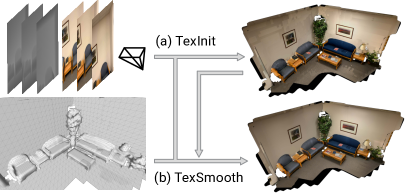
To address this robustness issue we find equipping of the recently-proposed adversarial texture optimization technique [24] with classical initialization and alignment techniques to be remarkably effective. Without the added initialization and alignment, we find current methods don’t produce high-quality textures. Concretely and as illustrated in Fig. 1, we aim for texture generation which operates on a sequence of images and corresponding depth maps as well as their camera parameters. Moreover, we assume the 3D model to be given and fixed. Importantly, we consider a streaming setup, with all data obtained on the fly, and not further processed, e.g., via batch structure-from-motion. The setup is ubiquitous and the form of data can be acquired easily from consumer-grade devices these days, e.g., from a recent iPad or iPhone [1]. We aim to translate this data into texture maps. For this, we first flatten the triangle mesh using recent advances [41]. We then use a Markov Random Field (MRF) to resolve overlaps in flattened meshes for non-manifold-connected data. In a next step we determine the image frame from which to extract the texture of each mesh triangle using a simple optimization. We refer to this as TexInit, which permits to obtain a high-quality initialization for subsequent refinement. Next we address inaccuracies in camera poses and in geometry by automatically shifting images using the result of a fast Fourier transformation (FFT) [6]. The final optimized texture is obtained by integrating this FFT-alignment component into adversarial optimization [24]. We dub this stage TexSmooth. The obtained texture can be used in any 3D engine for downstream applications.

To study efficacy of the proposed framework we acquire 11 complex scenes using a recent iPad. We establish accuracy of the proposed technique to generate and use the texture by showing that the quality of rendered views is superior to prior approaches on these scenes. Quantitatively, our framework improves prior work by 7.8% and 11.1% relatively with respect to perceptual (LPIPS [53]) and sharpness ($S_{3}$ [47]) measurements respectively. Besides, our framework improves over baselines on ScanNet [11], demonstrating the ability to generalize.

2 Related Work

We aim for accurate recovery of texture for a reconstructed 3D scene from a sequence of RGBD images. For this, a variety of techniques have been proposed, which can be roughly categorized into four groups: 1) averaging-based; 2) warping-based; 3) learning-based; and 4) assignment-based. Averaging-based methods find all views within which a point is visible and combine the color observations. Warping-based approaches either distort or synthesize source images to handle mesh misalignment or camera drift. Learning-based ones learn the texture representation. Assignment-based methods attempt to find the best view and ‘copy’ the observation into a texture. We review these groups next:

Averaging-based: Very early work by Marshner [29] estimates the parameters of a bidirectional reflectance distribution function (BRDF) for every point on the texture map. To compute this estimation, all observations from the recorded images where the point is visible are used. Similar techniques have been investigated in subsequent work [9].

Similarly, to compute a texture map, [30] and [12] perform a weighted blending of all recorded images. The weights take visibility and other factors into account. The developed approaches are semi-automatic as they require an initial estimate of the camera orientations which is obtained from interactively selected point correspondences or marked lines. Multi-resolution textures [33], face textures [36] and blending [31, 8] have also been studied.

Warping-based: Aganj et al. [4] morph each source image to align to the mesh. Furthermore, [54, 23] propose to optimize camera poses and image warping parameters jointly. However, this line of vertex-based optimization has stringent requirements on the mesh density and cannot be applied to a sparse mesh. More recently, Bi et al. [10] follow patch-synthesis [50, 7] to re-synthesize aligned target images for each source view. However, such methods require costly multiscale optimization to avoid a large number of local optima. In contrast, the proposed approach does not require those techniques.

Learning-based: Recently, learning-based methods have been introduced for texture optimization. Some works focus on specific object and scene categories [18, 40] while we do not make such assumptions. Moreover, learned representations, e.g., neural textures, have also been developed [46, 44, 5]. Meanwhile, generative models are developed to synthesize a holistic texture from a single image or pattern [21, 32] while we focus on texture reconstruction. AtlasNet [20] and NeuTex [52] focus on learning a 3D-to-2D mapping, which can be utilized in texture editing, while we focus on reconstructing realistic textures from source images. The recently-proposed adversarial texture optimization [24] utilizes adversarial training to reconstruct the texture. However, despite advances, adversarial optimization still struggles with misalignments. We improve this shortcoming via an explicit high-quality initialization and an efficient alignment module.

Assignment-based: Classical assignment-based methods operated within controlled environments [38, 39, 14, 15] or utilized special camera rigs [15, 19]. These works suggest computing for each vertex a set of ‘valid’ images, which are subsequently refined by iterating over each vertex and adjusting the assignment to obtain more consistency. Finally, texture data is ‘copied’ from the images. In contrast, we aim to create a texture in an uncontrolled setting. Consequently, 3D geometry is not accurate and very noisy. Other early work [13, 28, 22, 51, 39] focuses on closed surfaces and small-scale meshes, making them not applicable to our setting. More recently, upon finding the best texture independently for each face using cues like visibility, orientation, resolution, and distortion, refinement techniques like texture coordinate optimization, color adjustments, or scores-based optimization have been discussed [34, 48, 3].

Figure 2: Noisy geometry. The wall has two layers.

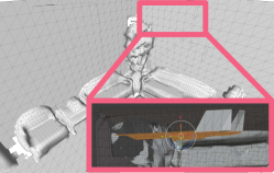
Related to our approach are methods that formulate texture selection using a Markov Random Field (MRF) [27, 42, 16]. Shu et al. [42] suggest visibility as the data term and employ texture smoothness to reduce transitions. Lempitsky et al. [27] study color-continuity which integrates over face seams. Fu et al. [16] additionally use the projected 2D face area to select a texture assignment for each face. However, noisy geometry like the one shown in Fig. 2, makes it difficult for assignment-based methods to yield high quality results, which we will show later. Therefore, different from these methods, we address texture drift in a data-driven refinement procedure rather than in an assignment stage.

3 Approach

We want to automatically create the texture ${\cal T}$ from a set of RGBD images $I=\{I_{1},\dots,I_{T}\}$, for each of which we also know camera parameters $\{p_{t}\}_{t=1}^{T}$, i.e., extrinsics and intrinsics. We are also given a triangular scene mesh $M=\left\{\texttt{Tri}_{i}\right\}_{i=1}^{|M|}$, where $\texttt{Tri}_{i}$ denotes the $i$-th triangle. This form of data is easily accessible from commercially available consumer devices, e.g., a recent iPhone or iPad.

We construct the texture ${\cal T}$ in two steps that combine advantages of assignment-based and learning-based techniques: 1) TexInit: we generate a texture initialization ${\cal T}_{\text{init}}\in\mathbb{R}^{H\times W\times 3}$ of height $H$, width $W$ and $3$ color channels in an assignment-based manner (Sec. 3.1); 2) TexSmooth: we then refine ${\cal T}_{\text{init}}$ with an improved data-driven adversarial optimization that integrates an efficient alignment procedure (Sec. 3.2). Formally, the final texture ${\cal T}$ is computed via

$${\cal T}=\texttt{TexSmooth}\left({\cal T}_{\text{init}},\{I_{t}\}_{t=1}^{T},\{p_{t}\}_{t=1}^{T},M\right),$$

where $${\cal T}_{\text{init}}=\texttt{TexInit}\left(\{I_{t}\}_{t=1}^{T},\{p_{t}\}_{t=1}^{T},M\right).$$ (1)

We detail each component next.

3.1 Texture Initialization (TexInit)

The proposed approach to obtain the texture initialization ${\cal T}_{\text{init}}$ is outlined in Fig. 3 and consists of following three steps: 1) We flatten the provided mesh $M$. For this we detect overlaps within the flattened mesh, which may happen due to the fact that we operate with general meshes that are not guaranteed to have a manifold connectivity. Overlap detection ensures that every triangle is assigned a unique position in the texture. 2) We identify for each triangle the ‘best’ texture index ${\bf t}^{\ast}$. Hereby, ‘best’ is defined using cues like visibility and color consistency. 3) After identifying the index ${\bf t}^{\ast}=(t_{1}^{\ast},\dots,t_{|M|}^{\ast})$ for each triangle, we create the texture ${\cal T}_{\text{init}}$ by transferring for all $(u,v)\in[1,\dots,W]\times[1,\dots,H]$ locations in the texture, the RGB data from the corresponding location $(a,b)$ in image $I_{t}$.

Figure 3: Texture initialization TexInit (Sec. 3.1). (a) Mesh flattening: we flatten a 3D mesh into the 2D plane using overlap detection. (b) Triangle-image assignment: we develop a simple formulation to compute the triangle-image assignment ${\bf t}^{\ast}$ from mesh $M$, frames $I_{t}$ and camera parameters $p_{t}$. We assign frames to each triangle $\texttt{Tri}_{i}$ based on ${\bf t}^{\ast}$. (c) Color transfer: based on the flattened mesh in (a) and the best assignment ${\bf t}^{\ast}$ from (b), we generate the texture ${\cal T}_{\text{init}}$.

1) Mesh Flattening:white1) Mesh Flattening: In a first step, as illustrated in Fig. 3 (left), we flatten the given mesh $M$. For this we use the recently proposed boundary first flattening (BFF) technique [41]. The flattening is fully automatic, with distortion mathematically guaranteed to be as low or lower than any other conformal mapping.

However, despite those guarantees, BFF still requires meshes to have a manifold connectivity. While we augment work by [41] using vertex duplication to circumvent this restriction, flattening may still result in overlapping regions as illustrated in Fig. 5. To fix this and uniquely assign a triangle to a position in the texture, we perform overlap detection as discussed next.

Overlap Detection: Overlap detection operates on flattened and possibly overlapping triangle meshes like the one illustrated in Fig. 4(a). Our goal is to assign triangles to different planes. Upon re-packing the triangles assigned to different planes, we obtain the non-overlapping triangle mesh illustrated in Fig. 4(b).

In order to not break the triangle mesh at a random position and end up with many individual triangles, i.e., in order to maintain large triangle connectivity, we formulate this problem using a Markov Random Field (MRF). Formally, let the discrete variable $y_{i}\in{\cal Y}=\{1,\dots,|{\cal Y}|\}$ denote the discrete plane index that the $i$-th triangle $\texttt{Tri}_{i}$ is assigned to. Hereby, $|{\cal Y}|$ denotes the maximum number of planes which is identical to the maximum number of triangles that overlap initially at any one location. We obtain the triangle-plane assignment $y^{\ast}=(y_{1}^{\ast},\dots,y_{|M|}^{\ast})$ for all $|M|$ triangles by addressing

$$y^{\ast}=\arg\max_{y}\sum_{i=1}^{|M|}\phi_{i}(y_{i})+\sum_{(i,j)\in{\cal A}\cup{\cal O}}\phi_{i,j}(y_{i},y_{j}),$$ (2)

where ${\cal A}$ and ${\cal O}$ are sets of triangle index pairs which are adjacent and overlapping respectively. Here, $\phi_{i}(\cdot)$ denotes triangle $\texttt{Tri}_{i}$’s priority over ${\cal Y}$ when considering only its local information, while $\phi_{i,j}(\cdot)$ refers to $\texttt{Tri}_{i}$ and $\texttt{Tri}_{j}$’s joint preference on their assignments. Eq. (2) is solved with belief propagation [17].

Intuitively, by addressing the program given in Eq. (2) we want a different plane index for overlapping triangles, while encouraging mesh $M$’s adjacent triangles to be placed on the same plane. To achieve this we use

$$\phi_{i}(y_{i}) =\begin{cases}1.0,&\text{if }y_{i}=\min{\cal Y}_{i,\text{non-overlap}}\\ 0.0,&\text{otherwise}\end{cases},\text{~{}and}$$ (3)

$$\phi_{i,j}(y_{i},y_{j}) =\begin{cases}\mathbbm{1}\{y_{i}=y_{j}\},&\text{if }(i,j)\in{\cal A}\\ \mathbbm{1}\{y_{i}\neq y_{j}\},&\text{if }(i,j)\in{\cal O}\end{cases}.$$ (4)

Here, $\mathbbm{1}\{\cdot\}$ denotes the indicator function and ${\cal Y}_{i,\text{non-overlap}}$ contains all plane indices where $\texttt{Tri}_{i}$ has no overlap with others. Intuitively, Eq. (3) encourages to assign the minimum of such indices to $\texttt{Tri}_{i}$.

(a) Flattened mesh overlaps.

(b) Overlap-free.

Figure 4: Flattening. (a) Red triangles indicate where overlap happens. (b) The proposed method (Sec. 3.1) resolves this issue while keeping connectivity of areas.

(c) L2Avg.

(d) ${\cal T}_{\text{init}}$.

Figure 5: Initialization comparison. (a) We use PyTorch3D’s rendering pipeline [37] to project each pixel of every RGB image back to the texture. The color of each pixel in the texture is the average of all colors that project to it. This texture minimizes the $\mathcal{L}_{2}$ loss of the difference between the rendered and the ground truth images. We dub it L2Avg. (b) ${\cal T}_{\text{init}}$ from Sec. 3.1 permits to maintain details. The seam artifacts will be optimized out using TexSmooth (Sec. 3.2). Besides over-smoothness, without taking into account misalignments of geometry and camera poses, L2Avg produces texture that overfits to available views, e.g., the sofa’s blue colors are painted onto the wall.

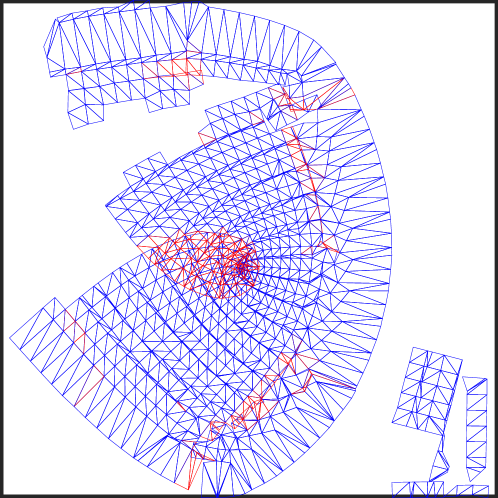
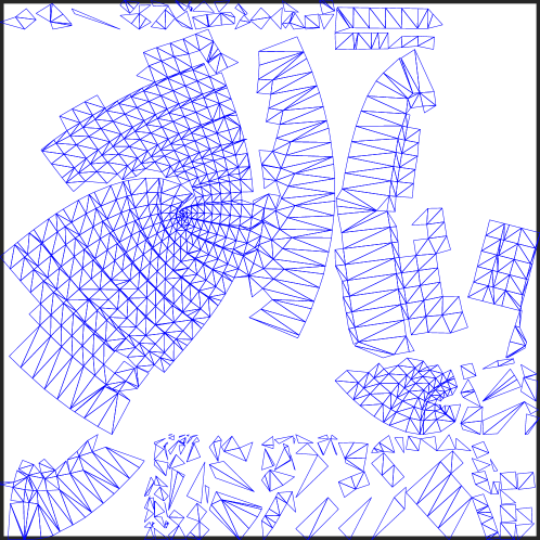
As fast MRF optimizers remove most overlaps but don’t provide guarantees, we add a light post-processing to manually assign the remaining few overlapping triangles to separate planes. This guarantees overlap-free results. As mentioned before, after having identified the plane assignment $y^{\ast}$ for each triangle we use a bin packing to uniquely assign each triangle to a position in the texture. Conversely, for every texture coordinate $u,v$ we obtain a unique triangle index

$$i=G(u,v).$$ (5)

A qualitative result is illustrated in Fig. 4(b). Next, we identify the image which should be used to texture each triangle.

2) Textures from Triangle-Image Assignments:white2) Textures from Triangle-Image Assignments: Our goal is to identify a suitable frame $I_{t_{i}}$, $t_{i}\in\{1,\dots,T+1\}$, for each triangle $\texttt{Tri}_{i}$, $i\in\{1,\dots,|M|\}$. Note that the $(T+1)$-th option $I_{T+1}$ refers to an empty texture. We compute the texture assignments ${\bf t}^{\ast}=(t_{1}^{\ast},\dots,t_{|M|}^{\ast})$ using a purely local optimization:

$${\bf t}^{\ast}=\mathop{\mathrm{argmax}}_{\bf t}\sum_{i=1}^{|M|}\psi_{i}(t_{i}).$$ (6)

Here $\psi_{i}$ captures unary cues. Note, we also studied pairwise cues but did not observe significant improvements. Please see the Appendix for more details. Due to better efficiency, we therefore only consider unary cues. Intuitively, we want the program given in Eq. (6) to encourage triangle-image assignment to be ‘best’ for each triangle $\texttt{Tri}_{i}$. We describe the unary cues to do so next.

Figure 6: Texture smoothing TexSmooth (Sec. 3.2). We utilize adversarial optimization (AdvOptim) [24] to refine the texture ${\cal T}_{\text{init}}$ from Sec. 3.1. Differently: 1) We initialize with ${\cal T}_{\text{init}}$. 2) To resolve the issue of misalignment between rendering and ground truth (GT), we integrate an alignment module based on the fast Fourier transform (FFT).

Unary Potentials $\psi_{i}(t_{i})$ for each pair of triangle $\texttt{Tri}_{i}$ and frame $I_{t_{i}}$ are

$$\psi_{i}(t_{i}) =\begin{cases}\psi_{i}^{\texttt{C}}(t_{i}),&\text{if }\psi_{i}^{\texttt{V}}(t_{i})=1\\ -\infty,&\text{otherwise}\end{cases},$$ (7)

where $\psi_{i}^{\texttt{V}}(t_{i})$ and $\psi_{i}^{\texttt{C}}(t_{i})$ represent validity check and potentials from cues respectively. Concretely, we use

$$\psi_{i}^{\texttt{V}}(t_{i}) =\mathbbm{1}\{I_{t_{i}}\in\mathcal{S}_{i}^{\texttt{V}}\},$$ (8)

$$\psi_{i}^{\texttt{C}}(t_{i}) =\omega_{1}\cdot\psi_{i}^{\texttt{C}_{1}}(t_{i})+\omega_{2}\cdot\psi_{i}^{\texttt{C}_{2}}(t_{i})+\omega_{3}\cdot\psi_{i}^{\texttt{C}_{3}}(t_{i}),$$ (9)

where $\mathcal{S}_{i}^{\texttt{V}}$ denotes the set of valid frames for $\texttt{Tri}_{i}$ and $\omega_{1},\omega_{2},\omega_{3}$ represent weights for potentials $\psi_{i}^{\texttt{C}_{1}},\psi_{i}^{\texttt{C}_{2}},\psi_{i}^{\texttt{C}_{3}}$. We discuss each one next:

$\bullet$ Validity (V). To assess whether frame $I_{t_{i}}$ is valid for $\texttt{Tri}_{i}$, we check the visibility of $\texttt{Tri}_{i}$ in $I_{t_{i}}$. We approximate this by checking visibility of $\texttt{Tri}_{i}$’s three vertices as well as its centroid. Concretely, we transform the vertices and centroid from world coordinates to the normalized device coordinates of the $t_{i}$-th camera. If all vertices and centroid are visible, i.e., their coordinates are in the interval $[-1,1]$, we add frame $I_{t_{i}}$ to the set $\mathcal{S}_{i}^{\texttt{V}}$ of valid frames for triangle $\texttt{Tri}_{i}$.

$\bullet$ Triangle area ($\texttt{C}_{1}$). Based on a camera’s pose $p_{t_{i}}$, a triangle’s area changes. The larger the area, the more detailed is the information for $\texttt{Tri}_{i}$ in frame $I_{t_{i}}$. We encourage to assign $\texttt{Tri}_{i}$ to frames $I_{t_{i}}$ with large area by defining $\psi_{i}^{\texttt{C}_{1}}(t_{i})=\texttt{Area}_{t_{i}}(\texttt{Tri}_{i})$ and set $\omega_{1}>0$.

$\bullet$ Discrepancy between $z$-buffer and actual depth ($\texttt{C}_{2}$). For a valid frame $I_{t_{i}}\in\mathcal{S}_{i}^{\texttt{V}}$, a triangle’s vertices and its centroid project to valid image coordinates. We compute the discrepancy between: 1) the depth from frame $I_{t_{i}}$ at the image coordinates of the vertices and centroid; 2) the depth of vertices and centroid in the camera’s coordinate system. We set $\psi_{i}^{\texttt{C}_{2}}(t_{i})$ to be the sum of absolute value differences between both depth estimates while using $\omega_{2}<0$.

$\bullet$ Perceptual consistency ($\texttt{C}_{3}$). Due to diverse illumination, triangle $\texttt{Tri}_{i}$’s appearance changes across frames. Intuitively, we don’t want to assign a texture to $\texttt{Tri}_{i}$ using a frame that contains colors that deviate drastically from other frames. Concretely, we first average all triangle’s three vertices color values across all valid frames, i.e., across all $I_{t_{i}}\in\mathcal{S}_{i}^{\texttt{V}}$. We then compare this global average to the local average obtained independently for the three vertices of every valid frame $I_{t_{i}}\in\mathcal{S}_{i}^{\texttt{V}}$ using an absolute value difference. We require $\omega_{3}<0$.

3) Color Transfer:white3) Color Transfer: Given the inferred triangle-frame assignments ${\bf t}^{\ast}$ we complete the texture ${\cal T}_{\text{init}}$ by transferring RGB data from image $I_{t_{i}^{\ast}}$ for $\texttt{Tri}_{i},i\in\{1,\dots,|M|\}$. For this we leverage the camera pose $p_{t_{i}^{\ast}}$ which permits to transform the texture coordinates $(u,v)$ of locations within $\texttt{Tri}_{i}$ to corresponding image coordinates $(a,b)$ in texture $I_{t_{i}^{\ast}}$ via the mapping $F:\mathbb{R}^{2}\rightarrow\mathbb{R}^{2}$, i.e.,

$$(a,b)=F(u,v,t_{i}^{\ast},p_{t_{i}^{\ast}}).$$ (10)

Intuitively, given the $(u,v)$ coordinates on the texture in a coordinate system which is local to the triangle $\texttt{Tri}_{i}$, and given the camera pose $p_{t_{i}^{\ast}}$ used to record image $I_{t_{i}^{\ast}}$, the mapping $F$ retrieves the image coordinates $(a,b)$ corresponding to texture coordinate $(u,v)$. Using this mapping, we obtain the texture ${\cal T}_{\text{init}}$ at location $(u,v)$, i.e., ${\cal T}_{\text{init}}(u,v)$, from the image data $I_{t_{i}^{\ast}}(a,b)\in\mathbb{R}^{3}$ via

$${\cal T}_{\text{init}}(u,v)=I_{t_{i}^{\ast}}(F(u,v,t_{i}^{\ast},p_{t_{i}^{\ast}})).$$ (11)

Note, because of the overlap detection, we obtain a unique triangle index $i=G(u,v)$ for every $(u,v)$ coordinate from Eq. (5). Having transferred RGB data for all coordinates within all triangles results in the texture ${\cal T}_{\text{init}}\in\mathbb{R}^{H\times W\times 3}$, which we compare to standard L2 averaging initialization in Fig. 5. We next refine this texture via adversarial optimization. We observe that this initialization ${\cal T}_{\text{init}}$ is crucial to obtain high-quality textures, which we will show in Sec. 4.

3.2 Texture Smoothing (TexSmooth)

As can be seen in Fig. 4(d), the texture ${\cal T}_{\text{init}}$ contains seams that affect visual quality. To reconstruct a seamless texture ${\cal T}$, we extend recent adversarial optimization (AdvOptim). Different from prior work [24] which initializes with blank (paper) or averaged (code release) textures, we initialize with ${\cal T}_{\text{init}}$. Also, we find AdvOptim doesn’t handle common camera pose and geometry misalignment well. To resolve this, we develop an efficient alignment module. This is depicted in Fig. 6 and will be detailed next.

Smoothing with Adversarial Optimization:whiteSmoothing with Adversarial Optimization: To optimize the texture, AdvOptim iterates over camera poses. When optimizing for a specific target camera pose $p_{\text{tar}}$, AdvOptim uses three images: 1) the ground truth image $I_{p_{\text{tar}}}$ of the target camera pose $p_{\text{tar}}$; 2) a rendering $\hat{I}_{p_{\text{tar}}}$ for the target camera pose $p_{\text{tar}}$ from the texture map ${\cal T}$; and 3) a re-projection from another camera pose $p_{\text{src}}$’s ground truth image, which we refer to as $I_{p_{\text{src}}\rightarrow p_{\text{tar}}}$. It then optimizes by minimizing an $\mathcal{L}_{1}$ plus a conditional adversarial loss. However, we find AdvOptim to struggle with alignment errors due to inaccurate geometry. Therefore, we integrate an efficient alignment operation into AdvOptim. Instead of directly using the input images, we first compute a 2D offset $(\Delta h_{p_{\text{tar}}},\Delta w_{p_{\text{tar}}})$ between $I_{p_{\text{tar}}}$ and $\hat{I}_{p_{\text{tar}}}$, which we apply to align $I_{p_{\text{tar}}}$ and $\hat{I}_{p_{\text{tar}}}$ as well as $I_{p_{\text{src}}\rightarrow p_{\text{tar}}}$ via

$$I^{\texttt{A}}\doteq\texttt{Align}(I,(\Delta h,\Delta w)),$$ (12)

where $I^{\texttt{A}}$ marks aligned images. We then use the three aligned images as input:

$$\mathcal{L}= \lambda\|I_{p_{\text{tar}}}^{\texttt{A}}-\hat{I}_{p_{\text{tar}}}^{\texttt{A}}\|_{1}+\mathbb{E}_{I_{p_{\text{tar}}}^{\texttt{A}},I_{p_{\text{src}}\rightarrow p_{\text{tar}}}^{\texttt{A}}}\left[\log D(I_{p_{\text{src}}\rightarrow p_{\text{tar}}}^{\texttt{A}}|I_{p_{\text{tar}}}^{\texttt{A}})\right]$$

$$+\mathbb{E}_{I_{p_{\text{tar}}}^{\texttt{A}},\hat{I}_{p_{\text{tar}}}^{\texttt{A}}}\left[\log(1-D(\hat{I}_{p_{\text{tar}}}^{\texttt{A}}|I_{p_{\text{tar}}}^{\texttt{A}}))\right].$$ (13)

Here, $D$ is a convolutional deep-net based discriminator. When using the unaligned image $I$ instead of $I^{\texttt{A}}$, Eq. (3.2) reduces to the vanilla version in [24]. We now discuss a fast way to align images.

Alignment with Fourier Transformation:whiteAlignment with Fourier Transformation: To align ground truth $I_{p_{\text{tar}}}$ and rendering $\hat{I}_{p_{\text{tar}}}$, one could use naïve grid-search to find the offset which results in the minimum difference of the shifted images. However, such a grid-search is prohibitively costly during an iterative optimization, especially with high-resolution images (e.g., we use a resolution up to 1920$\times$1440). Instead, we use the fast Fourier transformation (FFT) to complete the job [6]. Specifically, given a misaligned image pair of $I\in\mathbb{R}^{h\times w\times 3}$ and $\hat{I}\in\mathbb{R}^{h\times w\times 3}$, we compute for every channel the maximum correlation via

$$\mathop{\mathrm{argmax}}\limits_{(i,j)}\;\texttt{FFT}^{-1}\left(\texttt{FFT}(I)\cdot\overline{\texttt{FFT}(\hat{I})}\,\right)[i,j].$$ (14)

Here, $\texttt{FFT}(\cdot)$ represents the fast Fourier transformation while $\texttt{FFT}^{-1}(\cdot)$ denotes its inverse and $\overline{\texttt{FFT}(\hat{I})}$ refers to the complex conjugate. After decoding the maximum correlation response and averaging across channels, we obtain the final offset $(\Delta h,\Delta w)$. As can be seen in Fig. 8(d), the offset $(\Delta h,\Delta w)$ is very accurate. Moreover, the computation finishes in around 0.4 seconds even for $1920\times 1440$-resolution images. Note, we don’t need to maintain gradients for $(\Delta h,\Delta w)$, since the offset is only used to shift images and not to backpropagate through it.

Figure 7: Alignment with fast Fourier transformation (FFT) (Sec. 3.2). We show results for ${\cal T}_{\text{init}}$ (Sec. 3.1) and L2Avg (Fig. 5) in top and bottom rows. (a): ground-truth (GT); (b) and (e): texture rendering with (a)’s corresponding camera; (c) and (d): difference between (a) and (b); (f) and (g): difference between (a) and (e). The top row: FFT successfully aligns GT image and rendering from ${\cal T}_{\text{init}}$. Within expectation, there is almost no misalignment for the texture L2Avg as it overfits to available views (Fig. 5).

(a)

(b)

(c)

Figure 8: Alignment is important for evaluation (Sec. 4.1). Clearly, (c) is more desirable than (b). However, before alignment, LPIPS yields 0.3347 and 0.4971 for (a)-(b) and (a)-(c) pairs respectively. This is misleading as lower LPIPS indicates higher quality. After alignment, LPIPS produces 0.3343 and 0.2428 for the same pairs, which provides correct signals for evaluation.

4 Experiments

4.1 Experimental Setup

Data Acquisition. We use a 2020 iPad Pro and develop an iOS app to acquire the RGBD images $I_{t}$, camera pose $p_{t}$, and scene mesh $M$ via Apple’s ARKit [1].

UofI Texture Scenes. We collect a dataset of 11 scenes: four indoor and seven outdoor scenes. This dataset consists of a total of 2807 frames, of which 91, 2052, and 664 are of resolution $480\times 360$, $960\times 720$, and $1920\times 1440$ respectively. For each scene, we use 90% of its views for optimization and the remainder for evaluation. In total, we have 2521 training frames and 286 test frames. This setting is more challenging than prior work where [24] “select(s) 10 views uniformly distributed from the scanning video” for evaluation while using up to thousands of frames for texture generation. On average, the angular differences between test set view directions and their nearest neighbour in the training sets are 2.05^∘ (min 0.85^∘/max 13.8^∘). Angular distances are computed following [25]. Please see Appendix for scene-level statistics.

Implementation. We compare to five baselines for texture generation: L2Avg, ColorMap [54], TexMap [16], MVSTex [48], and AdvTex [24]. For ColorMap, TexMap, and MVSTex, we use their official implementations. For AdvOptim (Sec. 3.2) used in both AdvTex and ours, we re-implement a PyTorch [35] version based on their official release in TensorFlow [2].Footnote 1 We evaluate AdvTex with two different initializations: 1) blank textures as stated in the paper (AdvTex-B); 2) the initialization used in the official code release (AdvTex-C). We run AdvOptim using the Adam optimizer [26]. See Appendix for more details. For our TexInit (Sec. 3.1), we use a generic set of weights across all scenes: $\omega_{1}=1e^{-3}$ (triangle area), $\omega_{2}=-10$ (depth discrepancy), and $\omega_{3}=-1$ (perception consistency), which makes cue magnitudes roughly similar.

On a 3.10GHz Intel Xeon Gold 6254 CPU, ColorMap takes less than two minutes to complete while TexMap’s running time ranges from 40 minutes to 4 hours. MVSTex can be completed in no more than 10 minutes. Our ${\cal T}_{\text{init}}$ (Sec. 3.1) completes in two minutes. Additionally, the AdvOptim takes around 20 minutes for 4000 iterations to complete with an Nvidia RTX A6000 GPU.

Evaluation metrics. To assess the efficacy of the method, we study the quality of the texture from two perspectives: perceptual quality and sharpness. 1) For perceptual quality, we assess the similarity between rendered and collected ground-truth views using the Structural Similarity Index Measure (SSIM) [49] and the Learned Perceptual Image Patch Similarity (LPIPS) [53]. 2) For sharpness, we consider measurement $S_{3}$ [47] and the norm of image gradient (Grad) following [24]. Specifically, for each pixel, we compute its $S_{3}$ value, whose difference between the rendered and ground truth (GT) is used for averaging across the whole image. A similar procedure is applied to Grad. For all four metrics, we report the mean and standard deviation across 11 scenes.

Alignment in evaluation. As can be seen in Fig. 8, evaluation will be misleading if we do not align images during evaluation. Therefore, we propose the following procedure: 1) for each method, we align the rendered image and the GT using an FFT (Sec. 3.2); 2) to avoid various resolutions caused by different methods, we crop out the maximum common area across methods. 3) we then compute metrics on those cropped regions. The resulting comparison is fair as all methods are evaluated on the same number of pixels and aligned content.

4.2 Experimental Evaluation

Quantitative evaluation. Tab. 1 reports aggregated results on all 11 scenes. The quality of our texture ${\cal T}$ (Row 6) outperforms baselines on LPIPS, $S_{3}$ and Grad, confirming the effectiveness of the proposed pipeline. Specifically, we improve LPIPS by 7.8% from 0.335 ($2^{\text{nd}}$-best) to 0.309, indicating high perceptual similarity. Moreover, ${\cal T}$ maintains sharpness as we improve $S_{3}$ by 11.1% from 0.135 ($2^{\text{nd}}$-best) to 0.120 and Grad from 7.171 ($2^{\text{nd}}$-best) to 6.871. Regarding SSIM, we find it to favor L2Avg in almost all scenes (see Appendix) which aligns with the findings in [53].

Ablation study. We verify the design choices of TexInit and TexSmooth in Tab. 2. 1) TexSmooth is required: we directly evaluate ${\cal T}_{\text{init}}$ and $1^{\text{st}}$ vs. $4^{\text{th}}$ row confirms the performance drop: -0.092 (SSIM), +0.033 (LPIPS), +0.021 ($S_{3}$), and +1.221 (Grad). 2) ${\cal T}_{\text{init}}$ is needed: we replace ${\cal T}_{\text{init}}$ with L2Avg as it performs better than ColorMap and TexMap in Tab. 1 and still incorporate FFT into AdvOptim. We observe inferior performance: -0.010 (SSIM), +0.023 (LPIPS), +0.010 ($S_{3}$) in $2^{\text{nd}}$ vs. $4^{\text{th}}$ row. 3) Alignment is important: we use the vanilla AdvOptim but initialize with ${\cal T}_{\text{init}}$. As shown in Tab. 2’s $3^{\text{rd}}$ vs. $4^{\text{th}}$ row, the texture quality drops by -0.043 (SSIM), +0.037 (LPIPS), +0.005 ($S_{3}$), and +0.373 (Grad).

Table 1: Aggregated quantitative evaluation on UofI Texture Scenes. We report results in the form of $\texttt{mean}{\scriptsize\pm\texttt{std}}$. Please see Fig. 9 for qualitative texture comparisons and Appendix C.1 for scene-level quantitative results.

SSIM$\uparrow$ LPIPS$\downarrow$ $S_{3}\downarrow$ Grad$\downarrow$ 1 L2Avg 0.610$\pm$0.191 0.386$\pm$0.116 0.173$\pm$0.105 7.066$\pm$4.575 2 ColorMap 0.553$\pm$0.193 0.581$\pm$0.132 0.234$\pm$0.140 7.969$\pm$5.114 3 TexMap 0.376$\pm$0.113 0.488$\pm$0.097 0.179$\pm$0.062 8.918$\pm$4.174 4 MVSTex 0.476$\pm$0.164 0.335$\pm$0.086 0.139$\pm$0.047 8.198$\pm$3.936 5-1 AdvTex-B 0.495$\pm$0.174 0.369$\pm$0.092 0.148$\pm$0.047 8.229$\pm$4.586 5-2 AdvTex-C 0.563$\pm$0.191 0.365$\pm$0.096 0.135$\pm$0.067 7.171$\pm$4.272   6 Ours 0.602$\pm$0.189 0.309$\pm$0.086 0.120$\pm$0.058 6.871$\pm$4.342

Table 2: Ablation study. We report results in the form of $\texttt{mean}{\scriptsize\pm\texttt{std}}$.

Adv Optim FFT Align ${\cal T}_{\text{init}}$ SSIM$\uparrow$ LPIPS$\downarrow$ $S_{3}\downarrow$ Grad$\downarrow$ 1 ✓ 0.510$\pm$0.175 0.342$\pm$0.060 0.141$\pm$0.052 8.092$\pm$4.488 2 ✓ ✓ 0.592$\pm$0.192 0.332$\pm$0.102 0.130$\pm$0.066 6.864$\pm$4.211 3 ✓ ✓ 0.559$\pm$0.196 0.346$\pm$0.082 0.125$\pm$0.057 7.244$\pm$4.359   4 ✓ ✓ ✓ 0.602$\pm$0.189 0.309$\pm$0.086 0.120$\pm$0.058 6.871$\pm$4.342

(a) L2Avg.

(b) ColorMap [54].

(c) TexMap [16].

(d) MVSTex [48]. It removes geometry, which is not desirable.

(e) AdvTex-C [24]. We highlight artifacts with boxes. 1) Scene 1: sofa’s texture is mapped to the wall and the figure on the wall is broken; 2) Scene 2: the door’s color is mapped to the floor and the brick wall’s pattern is mapped to light; 3) Scene 3: ball’s color is projected to brick walls; 4) Scene 4: bench’s color is added to the bush and ground; 5) Scene 5: the crack breaks and stair’s color is on the ground.

(f) Ours. Compared to Fig. 9(e), our method reduces artifacts.

(g) Highlights. From left to right and top to bottom, we show ground-truth image and renderings at the same camera pose with texture from ColorMap, TexMap, MVSTex, AdvTex-C, and ours respectively. Compared to AdvTex-C: 1) Scene 1: ours produces much more complete and sharper pattern for the sofa; 2) Scene 2: ours generates sharper cracks on brick walls; 3) Scene 3: our balls are more complete while AdvTex-C maps the top of the ball to the left brick wall; 4) Scene 4: AdvTex-C maps the bench to the bush while ours is much cleaner; 5) Scene 5: the pattern on the ground from ours is much sharper.

Figure 9: Qualitative results on UofI Texture Scenes. For each method, we show results for Scene 1 to 5 from left to right. Best viewed in color and zoomed-in.

Table 3: ScanNet results. We report results in the form of $\texttt{mean}{\scriptsize\pm\texttt{std}}$. Note, this can’t be directly compared to [23]’s Tab. 2: while we reserve 10% views for evaluation, [23] reserves only 10/2011 ($\approx$ 0.5%), where 2011 is the number of average views per scene.

SSIM$\uparrow$ LPIPS$\downarrow$ $S_{3}\downarrow$ Grad$\downarrow$ 1-1 AdvTex-B 0.534$\pm$0.074 0.557$\pm$0.071 0.143$\pm$0.028 3.753$\pm$0.730 1-2 AdvTex-C 0.531$\pm$0.074 0.558$\pm$0.075 0.161$\pm$0.044 4.565$\pm$1.399   2 Ours 0.571$\pm$0.069 0.503$\pm$0.090 0.127$\pm$0.031 3.324$\pm$0.826

Figure 10: Remaining six scenes with our textures. See Appendix for all methods’ results on these scenes.

Figure 11: Results on ScanNet. Left to right: AdvTex-B/C and ours. Ours alleviates artifacts: colors from box on the cabinet are mapped to the backpack and wall.

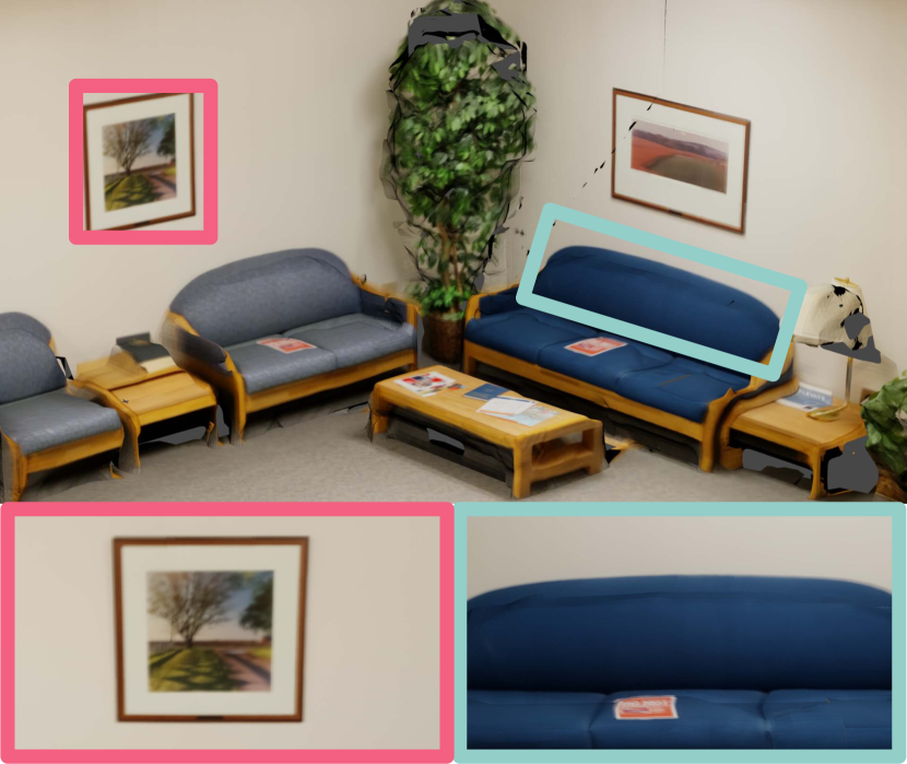
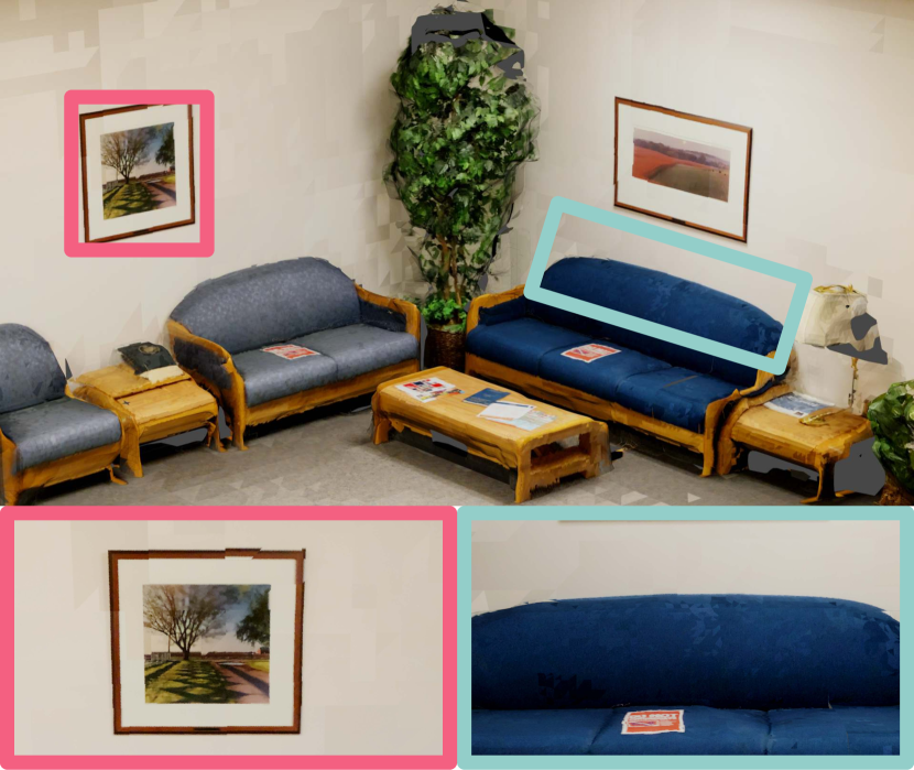
Qualitative evaluation. We present qualitative examples in Fig. 9. Fig. 9(a) and Fig. 9(b) demonstrate that L2Avg and ColorMap produce overly smooth texture. Meanwhile, due to noise in the geometry, e.g., Fig. 2, TexMap fails to resolve texture seams and cannot produce a complete texture (Fig. 9(c)). MVSTex results in Fig. 9(d) are undesirable as geometries are removed. This is because MVSTex requires ray collision checking to remove occluded faces. Due to the misalignment between geometries and cameras, artifacts are introduced. We show results of AdvTex-C in Fig. 9(e) as it outperforms AdvTex-B from Tab. 1. Artifacts are highlighted. Our method can largly mitigate such seams, which can be inferred from Fig. 9(f). 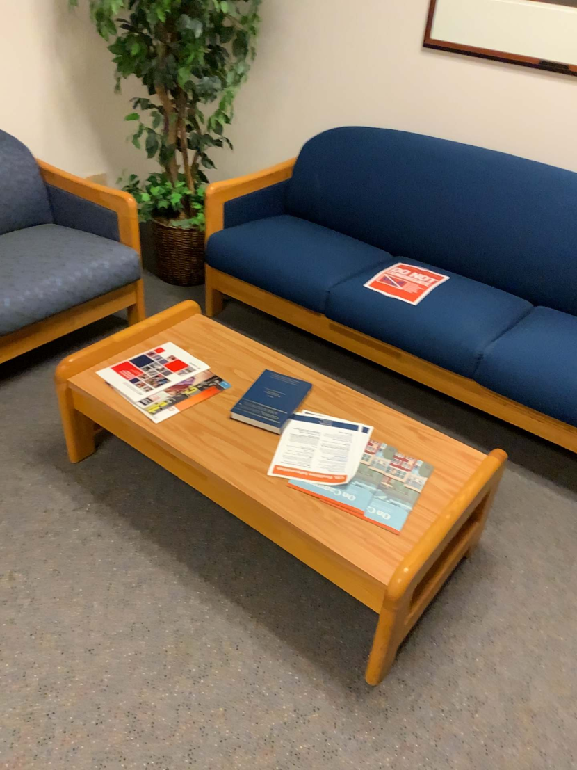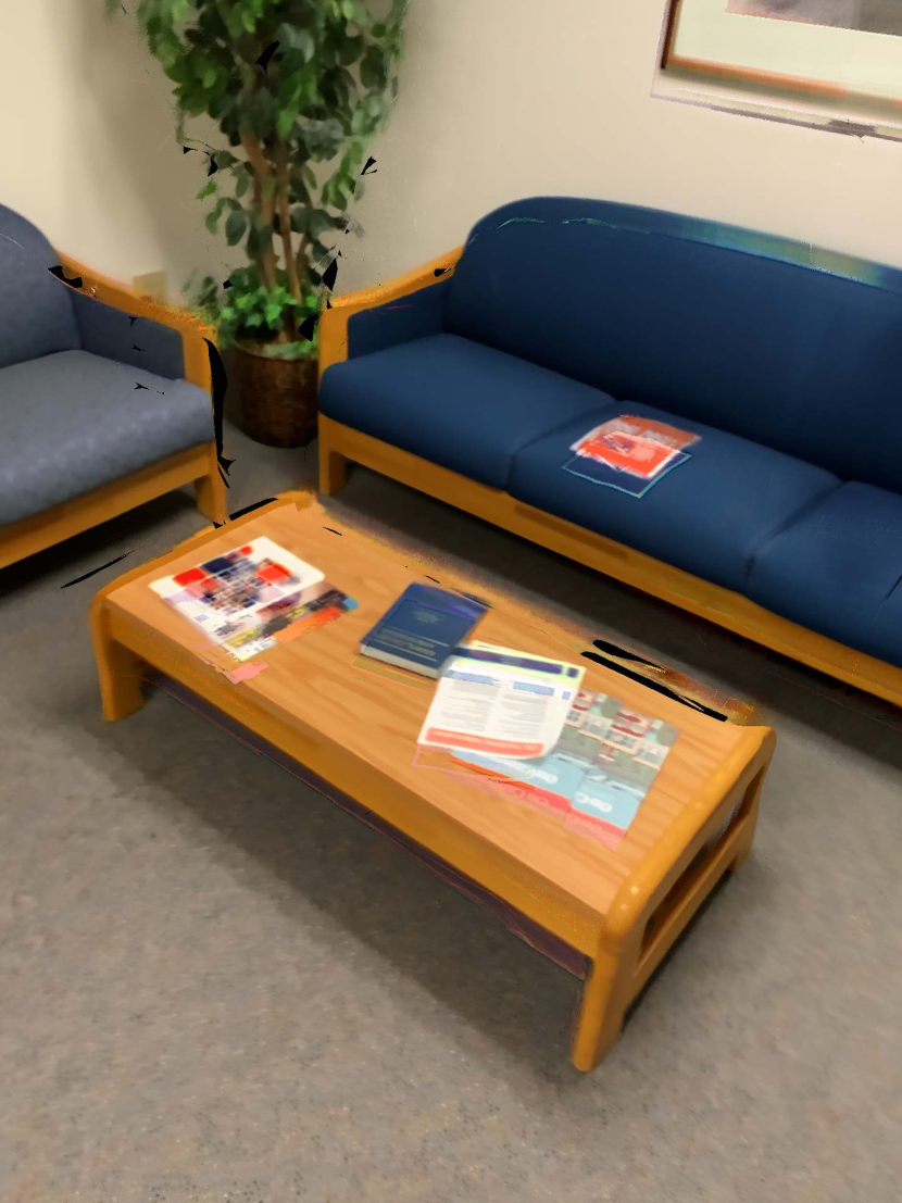In Fig. 9(g), we show renderings, which demonstrate the effectiveness of the proposed method. Please see Appendix for complete qualitative results of scenes in Fig. 11.

On ScanNet [11]. Following [24], we study scenes with ID $\leq$ 20 ( Fig. 11, Tab. 3). We improve upon baselines (AdvTex-B/C) by a margin on SSIM (0.534 $\rightarrow$ 0.571), LPIPS (0.557 $\rightarrow$ 0.503), $S_{3}$ (0.143 $\rightarrow$ 0.127), and Grad (3.753 $\rightarrow$ 3.324).

5 Conclusion

We develop an initialization and an alignment method for fully-automatic texture generation from a given scene mesh, and a given sequence of RGBD images and their camera parameters. We observe the proposed method to yield appealing results, addressing robustness issues due to noisy geometry and misalignment of prior work. Quantitatively we observe improvements on both perceptual similarity (LPIPS from 0.335 to 0.309) and sharpness ($S_{3}$ from 0.135 to 0.120).

Acknowledgements: Supported in part by NSF grants 1718221, 2008387, 2045586, 2106825, MRI #1725729, and NIFA award 2020-67021-32799.

Supplementary Material:
Initialization and Alignment
for Adversarial Texture Optimization

This supplementary is structured as follows:

• Sec. A provides details regarding the scenes;

• Sec. B describes implementation details;

• Sec. C provides more quantitative results;

• Sec. D gives more ablation studies;

• Sec. E shows more qualitative results.

Appendix A UofI Texture Scenes Details

We provide detailed scene statistics in Tab. S1. As mentioned in Sec. 4.1, we collect a dataset of 11 scenes: four indoor and seven outdoor scenes. This dataset consists of a total of 2807 frames, of which 91, 2052, and 664 are of resolution $480\times 360$, $960\times 720$, and $1920\times 1440$ respectively. For each scene, we reserve 10% of the views for evaluation. In contrast, prior work [24] “select(s) 10 views uniformly distributed from the scanning video” for evaluation while using up to thousands of frames for texture generation. The studied setting is hence more demanding.

Appendix B Implementation Details

B.1 Network Structure for TexSmooth

As mentioned in Sec. 3.2, we utilize a convolutional neural network for the discriminator $D$ in Eq. (3.2). Specifically, we follow [24]’s code release to utilize five convolutional layers with structures (6, 64, 2), (64, 128, 2), (128, 128, 2), (128, 128, 1), (128, 1, 1), where $(in,out,s)$ indicates the number of input channels, the number of output channels, and stride respectively. All layers employ a $4\times 4$ kernel and use VALID padding. Regarding activation functions, the first four layers contain leakyReLUs while the last one uses a sigmoid activation.

B.2 Hyperparameters

The weight for the $\mathcal{L}_{1}$ loss in Eq. (3.2) is $\lambda=10$. We decay it by a factor of 0.8 every 960 steps. We use Adam [26] with $\beta_{1}=0.5$ and $\beta_{2}=0.999$. The learning rates for the texture and discriminator are set to $1e^{-3}$ and $1e^{-4}$ respectively. We run AdvOptim for 4000 iterations for AdvTex-C and our TexSmooth stage, following the code release.Footnote 3 For AdvTex-B, AdvOptim runs for 50000 iterations as stated in their paper [24].

B.3 AdvOptim Reimplementation

As mentioned in Sec. 4.1, we re-implement AdvOptim using PyTorch based on the official TensorFlow (TF) code. To verify the correctness of our implementation, we compare results from the official code release and our re-implemented version on the Chair dataset from [24], which contains 35 scanned chairs. Specifically, similar to Sec. 4.1, we reserve 10% of the views from each scan for evaluation, resulting in 14,836 training views and 1663 test views. As can be seen from the $1^{\text{st}}$ vs. $2^{\text{nd}}$ row in Tab. S2, we observe 0.830 vs. 0.828 SSIM, 0.163 vs. 0.167 LPIPS, 0.068 vs. 0.069 $S_{3}$, and 2.052 vs. 2.047 Grad. This verifies the correctness of our re-implementation.

Table S1: Statistics of UofI Texture Scenes. For each column, the format is indicated below the header. We reserve 10% views for evaluation. “Angular Diff” measures the the angular differences between test set view directions and their nearest neighbour in the training sets.

	Mesh $\#$Faces	$\#$Views total (test)	Resolution value ($\#$count)	Angular Diff avg (min/max)
1	77,528	160 (16)	1920$\times$1440 (160)	2.04∘ (0.38∘/4.26∘)
2	104,684	195 (20)	960$\times$720 (195)	0.85∘ (0.06∘/2.46∘)
3	132,196	94 (10)	1920$\times$1440 (3) 480$\times$360 (91)	4.58∘ (1.14∘/13.8∘)
4	65,832	43 (5)	960$\times$720 (43)	3.48∘ (0.12∘/6.66∘)
5	143,108	584 (59)	960$\times$720 (584)	1.28∘ (0.19∘/3.18∘)
6	168,664	372 (38)	1920$\times$1440 (372)	1.45∘ (0.36∘/3.13∘)
7	77,627	233 (24)	960$\times$720 (233)	3.24∘ (0.67∘/12.6∘)
8	80,240	352 (36)	960$\times$720 (352)	1.60∘ (0.27∘/6.89∘)
9	199,976	347 (35)	960$\times$720 (347)	1.81∘ (0.21∘/4.55∘)
10	69,484	129 (13)	1920$\times$1440 (129)	1.12∘ (0.19∘/2.59∘)
11	149,176	298 (30)	960$\times$720 (298)	1.13∘ (0.27∘/2.60∘)

Table S2: Quantitative results on Chair dataset. We report in the form of $\texttt{mean}{\scriptsize\pm\texttt{std}}$.

		SSIM$\uparrow$	LPIPS$\downarrow$	$S_{3}\downarrow$	Grad$\downarrow$
1	TF	0.830$\pm$0.072	0.163$\pm$0.072	0.068$\pm$0.020	2.052$\pm$1.267
2	PyTorch	0.828$\pm$0.072	0.167$\pm$0.073	0.069$\pm$0.020	2.047$\pm$1.275
3	TexInit + TexSmooth	0.827$\pm$0.073	0.167$\pm$0.073	0.068$\pm$0.019	2.071$\pm$1.289

B.4 Determine ${\cal T}$ resolution

To determine the $H$ and $W$ of the texture ${\cal T}$, we use the following three steps: 1) for each of the $|{\cal Y}|$ planes mentioned in Sec. 3.1’s “Overlap Detection”, we use a resolution of $512^{2}$, $1024^{2}$, or $2048^{2}$ based on whether the major RGB resolution’s larger side is 480, 960, or 1920; 2) all $|{\cal Y}|$ planes are concatenated to obtain the texture ${\cal T}$’s $H$ and $W$; 3) For a fair comparison, AdvTex baselines use the same resolution as ours.

Appendix C More Quantitative Results

C.1 Scene-level Quantitative Results

We provide scene-level quantitative results in Tab. S5. As can be seen from the number for the Best or $2^{\text{nd}}$-Best results (last two rows), our technique improves upon all baselines. Specifically, ours dominates the count (ours vs. runner-up) for “best” (17 vs. 14), “2${}^{\text{nd}}$-best” (14 vs. 13), and “best or 2${}^{\text{nd}}$-best” (31 vs. 18).

C.2 Results on Existing Dataset

We apply our TexInit + TexSmooth on the Chair dataset. We directly utilize the provided conformal mapping to ensure a fair comparison. Quantitative results are shown in $2^{\text{nd}}$ vs. $3^{\text{rd}}$ row of Tab. S2. Our method performs on par with the baseline. This is expected as we do not observe geometry and images of those scans to be misaligned. Beneficially and as expected, the proposed technique doesn’t harm the result if geometry and images are well aligned.

C.3 Robustness to Inaccurate Camera Poses

To verify the robustness of the proposed pipeline, we conduct studies by deliberately adding more noise to camera poses in the training split. Concretely, given a camera pose with rotation $(r_{x},r_{y},r_{z})$ (represented in Euler angles) and translation $(t_{x},t_{y},t_{z})$, we add uniformly-sampled noise, i.e., we have $\widehat{r}_{x}=r_{x}+\epsilon_{r_{x}}$, where $\epsilon_{r_{x}}\sim\mathcal{U}(-0.05\cdot|r_{x}|,0.05\cdot|r_{x}|)$, and analogously $\widehat{r}_{y},\widehat{r}_{z},\widehat{t}_{x},\widehat{t}_{y},\widehat{t}_{z}$. We apply AdvTex-B/C and ours on data with these corrupted camera poses. Tab. S3 corroborates the robustness of the method: we outperform baselines on SSIM (0.456 vs. 0.452, $\uparrow$ is better), LPIPS (0.472 vs. 0.490, $\downarrow$ is better), and sharpness $S_{3}$ (0.142 vs. 0.153, $\downarrow$ is better).

Table S3: Evaluation with noise added to camera poses on UofI Texture Scenes. Results are in the form of $\texttt{mean}{\scriptsize\pm\texttt{std}}$. Ours is the most robust.

		SSIM$\uparrow$	LPIPS$\downarrow$	$S_{3}\downarrow$	Grad$\downarrow$
1-1	AdvTex-B	0.378$\pm$0.158	0.503$\pm$0.091	0.160$\pm$0.040	9.193$\pm$4.562
1-2	AdvTex-C	0.452$\pm$0.191	0.490$\pm$0.082	0.153$\pm$0.072	7.949$\pm$4.364
2	Ours	0.456$\pm$0.196	0.472$\pm$0.078	0.142$\pm$0.050	8.177$\pm$4.441

Appendix D More Ablations

D.1 Unary vs. Pairwise Cues

As stated in Eq. (6), we use pure-unary cues for TexInit. To verify this design choice, we ablate with a setup where TexInit considers both unary and pairwise cues. Concretely, we consider the following optimization problem:

$${\bf t}^{\ast}=\mathop{\mathrm{argmax}}_{\bf t}\sum_{i=1}^{|M|}\psi_{i}(t_{i})+\sum_{(i,j)\in{\cal A}}\psi_{i,j}(t_{i},t_{j}),$$ (S1)

where ${\cal A}$ is the adjacency used in Eq. (2). Here $\psi_{i}$ refers to the unary cues in Eq. (6) while $\psi_{i,j}$ captures pairwise ones. Therefore, besides $\texttt{C}_{1}$, $\texttt{C}_{2}$, and $\texttt{C}_{3}$ discussed in Sec. 3.1, we take into account another cue $\texttt{C}_{4}$:

$$\psi_{i,j}(t_{i},t_{j})\doteq\psi_{i,j}^{\texttt{C}_{4}}(t_{i},t_{j}).$$ (S2)

$\bullet$ Explicit adjacency encouragement ($\texttt{C}_{4}$). Intuitively, adjacent triangles $\texttt{Tri}_{i}$ and $\texttt{Tri}_{j}$ maintain smoothness if they are assigned textures from the same frame. We encourage this choice using $\psi_{i,j}^{\texttt{C}_{4}}(t_{i},t_{j})=\mathbbm{1}(t_{i}=t_{j})$ and set $\omega_{4}>0$.

In our experiments, we set $\omega_{4}=1$ for TexInit. The TexSmooth stage remains the same. Quantitative results are shown in Column 1-1 vs. 1-2 in Tab. S6. We do not observe a big difference when integrating pairwise cues. Concretely, when comparing pairwise vs. unary only cues, we have 0.601 vs. 0.602 (SSIM), 0.305 vs. 0.309 (LPIPS), 0.120 vs. 0.120 ($S_{3}$), and 6.872 vs. 6.871 (Grad), which corroborate our design.

D.2 View Sparsity Analysis

To understand whether our framework is sensitive to the sparsity of training views, we conduct an ablation: 1) we reserve 10% of the views, which are uniformly sampled, for evaluation. As a consequence, we have 90% of all views that can be used for training; 2) within those 90% of all views, we again uniformly sample images for optimization every $k$ views. We use $k\in\{1,2,3,4,5\}$. Note, the results reported in Tab. 1, Tab. 2, and Tab. S5 are situations where $k=1$, namely all 90% views are used. Quantitative results are reported in Column 1-1 to Column 5 in Tab. S6. As expected, when the number of training views decreases, we observe the results’ quality to drop. However, our framework is robust to the view sparsity as the performance gap is small. Specifically, we observe best vs. worst results as 0.604 vs. 0.580 (SSIM), 0.303 vs. 0.316 (LPIPS), 0.120 vs. 0.127 ($S_{3}$), and 6.859 vs. 7.026 (Grad). The reason that $k=2$ performs slightly better than $k=1$ is that 1) $k=2$ still provides dense enough views for TexInit and TexSmooth; 2) the initialization from TexInit can contain less seams as less views are considered.

D.3 Patchwise Alignment

We assess the results of patch-wise alignment in our pipeline. Tab. S4 and Fig. S1 verify: a patch-wise method ignores global content and is inferior.

Table S4: Patchwise alignment on UofI Texture Scenes. Results are in the form of $\texttt{mean}{\scriptsize\pm\texttt{std}}$. $X\times Y$ in the ‘#Patches’ column denotes the number of patches created by splitting along height ($X$) and width ($Y$). See Fig. S1 for qualitative results.

	#Patches	SSIM$\uparrow$	LPIPS$\downarrow$	$S_{3}\downarrow$	Grad$\downarrow$
1	$1\times 1$	0.602$\pm$0.189	0.309$\pm$0.086	0.120$\pm$0.058	6.871$\pm$4.342
2	$2\times 2$	0.556$\pm$0.184	0.330$\pm$0.069	0.123$\pm$0.055	7.122$\pm$4.306
3	$4\times 4$	0.545$\pm$0.175	0.338$\pm$0.064	0.122$\pm$0.054	7.163$\pm$4.257

Figure S1: Patch-wise alignment on UofI Texture Scenes. Highlighted issues: sofa and plant colors are mapped to the wall in (b,c).

Table S5: Scene-level quantitative results on UofI Texture Scenes. We use bold and underline to mark best and $2^{\text{nd}}$-best results for each row respectively. If one value’s difference from its higher-rank counterpart is no larger than 0.001, we treat them as the same.

1 2 3 4 5 6 7 8 9 10 L2Avg ColorMap TexMap MVSTex AdvTex-B AdvTex-C ${\cal T}_{\text{init}}$ Only w/o ${\cal T}_{\text{init}}$ w/o Align Ours Scene 1 SSIM$\uparrow$ 0.866 0.831 0.608 0.718 0.774 0.834 0.769 0.863 0.845 0.876 LPIPS$\downarrow$ 0.235 0.361 0.387 0.260 0.227 0.261 0.251 0.215 0.228 0.187 $S_{3}\downarrow$ 0.042 0.058 0.088 0.073 0.064 0.051 0.070 0.043 0.046 0.041 Grad$\downarrow$ 1.806 2.085 3.232 2.977 2.349 2.073 2.414 1.816 1.936 1.724 Scene 2 SSIM$\uparrow$ 0.584 0.428 0.384 0.494 0.486 0.541 0.521 0.592 0.532 0.626 LPIPS$\downarrow$ 0.319 0.653 0.433 0.221 0.288 0.290 0.271 0.231 0.294 0.226 $S_{3}\downarrow$ 0.227 0.342 0.253 0.172 0.172 0.180 0.190 0.165 0.174 0.164 Grad$\downarrow$ 8.910 11.09 11.75 10.28 9.909 9.499 9.749 8.488 9.707 8.067 Scene 3 SSIM$\uparrow$ 0.651 0.594 0.465 0.575 0.534 0.605 0.561 0.630 0.585 0.636 LPIPS$\downarrow$ 0.362 0.533 0.459 0.301 0.383 0.344 0.354 0.324 0.348 0.309 $S_{3}\downarrow$ 0.135 0.170 0.188 0.129 0.153 0.121 0.132 0.128 0.124 0.121 Grad$\downarrow$ 5.721 5.707 8.203 6.836 7.468 6.051 6.566 6.118 6.238 5.659 Scene 4 SSIM$\uparrow$ 0.217 0.182 0.168 0.155 0.133 0.187 0.176 0.198 0.180 0.244 LPIPS$\downarrow$ 0.656 0.845 0.468 0.370 0.575 0.540 0.430 0.516 0.500 0.440 $S_{3}\downarrow$ 0.310 0.441 0.168 0.112 0.152 0.143 0.118 0.141 0.128 0.121 Grad$\downarrow$ 16.79 18.35 16.68 15.78 18.05 16.07 16.76 15.95 16.13 16.09 Scene 5 SSIM$\uparrow$ 0.480 0.430 0.397 0.412 0.422 0.448 0.422 0.474 0.430 0.472 LPIPS$\downarrow$ 0.427 0.615 0.391 0.268 0.343 0.351 0.308 0.332 0.321 0.293 $S_{3}\downarrow$ 0.326 0.403 0.267 0.213 0.225 0.227 0.223 0.220 0.210 0.205 Grad$\downarrow$ 10.38 11.80 11.83 10.62 10.85 9.359 11.18 9.230 10.12 9.807 Scene 6 SSIM$\uparrow$ 0.684 0.615 0.330 0.392 0.509 0.598 0.480 0.637 0.591 0.642 LPIPS$\downarrow$ 0.374 0.615 0.674 0.553 0.386 0.403 0.419 0.343 0.408 0.363 $S_{3}\downarrow$ 0.058 0.099 0.122 0.109 0.129 0.066 0.127 0.064 0.075 0.067 Grad$\downarrow$ 3.020 3.552 4.925 4.790 4.500 3.435 4.476 3.360 3.551 3.256 Scene 7 SSIM$\uparrow$ 0.423 0.378 0.343 0.346 0.362 0.384 0.374 0.411 0.373 0.396 LPIPS$\downarrow$ 0.465 0.650 0.475 0.347 0.436 0.442 0.356 0.448 0.392 0.367 $S_{3}\downarrow$ 0.280 0.385 0.262 0.215 0.216 0.245 0.220 0.239 0.203 0.200 Grad$\downarrow$ 12.16 13.98 13.27 12.93 13.27 12.09 13.65 11.60 12.11 11.91 Scene 8 SSIM$\uparrow$ 0.846 0.808 0.265 0.629 0.679 0.815 0.740 0.839 0.816 0.842 LPIPS$\downarrow$ 0.269 0.498 0.680 0.396 0.328 0.286 0.349 0.259 0.278 0.250 $S_{3}\downarrow$ 0.060 0.084 0.135 0.117 0.096 0.063 0.080 0.058 0.060 0.055 Grad$\downarrow$ 2.062 2.489 4.627 4.405 3.181 2.275 2.877 2.070 2.257 2.011 Scene 9 SSIM$\uparrow$ 0.545 0.502 0.306 0.373 0.376 0.450 0.383 0.500 0.469 0.508 LPIPS$\downarrow$ 0.483 0.709 0.509 0.371 0.460 0.520 0.419 0.474 0.454 0.451 $S_{3}\downarrow$ 0.194 0.254 0.197 0.146 0.146 0.163 0.132 0.159 0.138 0.143 Grad$\downarrow$ 6.988 8.042 9.815 8.751 8.582 7.514 8.380 6.765 6.985 6.814 Scene 10 SSIM$\uparrow$ 0.853 0.800 0.493 0.718 0.716 0.810 0.744 0.828 0.816 0.839 LPIPS$\downarrow$ 0.260 0.403 0.492 0.305 0.282 0.244 0.267 0.204 0.240 0.198 $S_{3}\downarrow$ 0.043 0.059 0.088 0.072 0.099 0.051 0.081 0.047 0.049 0.045 Grad$\downarrow$ 2.159 2.476 3.740 3.366 3.295 2.564 3.081 2.416 2.421 2.283 Scene 11 SSIM$\uparrow$ 0.563 0.520 0.374 0.428 0.454 0.518 0.443 0.546 0.513 0.544 LPIPS$\downarrow$ 0.398 0.510 0.399 0.292 0.350 0.337 0.334 0.307 0.345 0.312 $S_{3}\downarrow$ 0.229 0.278 0.198 0.167 0.178 0.177 0.179 0.165 0.167 0.158 Grad$\downarrow$ 7.742 8.100 10.04 9.435 9.057 7.946 9.878 7.684 8.225 7.957 Count Best 14 0 0 9 0 1 1 5 0 17 $2^{\text{nd}}$-Best 4 1 0 0 0 2 4 13 3 14

Table S6: Scene-level ablation results on UofI Texture Scenes. The fractions below each header indicate the portion of training views utilized during optimization. Note, we do not consider the already-reserved 10% views for evaluation. Namely, $1/1$ means we use all 90% training views. For Column 1-1, we use pairwise cues for TexInit while only unary cues are utilized for the remaining columns. We report $\texttt{mean}{\scriptsize\pm\texttt{std}}$.

		1-1	1-2	2	3	4	5
		1/1-pairwise	1/1	1/2	1/3	1/4	1/5
Scene 1	SSIM$\uparrow$	0.876	0.876	0.873	0.868	0.831	0.826
	LPIPS$\downarrow$	0.186	0.187	0.185	0.187	0.216	0.213
	$S_{3}\downarrow$	0.040	0.041	0.042	0.044	0.058	0.063
	Grad$\downarrow$	1.727	1.724	1.742	1.770	2.045	2.120
Scene 2	SSIM$\uparrow$	0.622	0.626	0.624	0.617	0.614	0.610
	LPIPS$\downarrow$	0.219	0.226	0.218	0.215	0.221	0.215
	$S_{3}\downarrow$	0.162	0.164	0.160	0.161	0.161	0.159
	Grad$\downarrow$	8.070	8.067	8.053	8.105	8.162	8.124
Scene 3	SSIM$\uparrow$	0.637	0.636	0.657	0.630	0.601	0.639
	LPIPS$\downarrow$	0.307	0.309	0.293	0.312	0.314	0.265
	$S_{3}\downarrow$	0.120	0.121	0.117	0.125	0.133	0.112
	Grad$\downarrow$	5.639	5.659	5.445	5.706	6.008	5.435
Scene 4	SSIM$\uparrow$	0.237	0.244	0.258	0.240	0.219	0.204
	LPIPS$\downarrow$	0.442	0.440	0.440	0.444	0.466	0.417
	$S_{3}\downarrow$	0.123	0.121	0.122	0.128	0.128	0.114
	Grad$\downarrow$	16.21	16.09	16.09	16.33	16.00	16.45
Scene 5	SSIM$\uparrow$	0.473	0.472	0.471	0.473	0.473	0.474
	LPIPS$\downarrow$	0.294	0.293	0.288	0.288	0.290	0.287
	$S_{3}\downarrow$	0.206	0.205	0.205	0.205	0.205	0.203
	Grad$\downarrow$	9.853	9.807	9.866	9.830	9.850	9.889
Scene 6	SSIM$\uparrow$	0.644	0.642	0.643	0.627	0.621	0.618
	LPIPS$\downarrow$	0.364	0.363	0.351	0.351	0.355	0.353
	$S_{3}\downarrow$	0.066	0.067	0.070	0.073	0.074	0.073
	Grad$\downarrow$	3.245	3.256	3.284	3.349	3.375	3.352
Scene 7	SSIM$\uparrow$	0.400	0.396	0.407	0.400	0.400	0.411
	LPIPS$\downarrow$	0.367	0.367	0.368	0.366	0.366	0.354
	$S_{3}\downarrow$	0.201	0.200	0.199	0.200	0.201	0.194
	Grad$\downarrow$	11.88	11.91	11.74	11.94	11.93	11.62
Scene 8	SSIM$\uparrow$	0.837	0.842	0.827	0.816	0.814	0.815
	LPIPS$\downarrow$	0.249	0.250	0.257	0.271	0.270	0.268
	$S_{3}\downarrow$	0.055	0.055	0.060	0.065	0.065	0.065
	Grad$\downarrow$	2.035	2.011	2.115	2.209	2.224	2.224
Scene 9	SSIM$\uparrow$	0.509	0.508	0.506	0.498	0.490	0.489
	LPIPS$\downarrow$	0.440	0.451	0.441	0.441	0.441	0.428
	$S_{3}\downarrow$	0.143	0.143	0.142	0.141	0.142	0.140
	Grad$\downarrow$	6.788	6.814	6.787	6.844	6.886	6.852
Scene 10	SSIM$\uparrow$	0.839	0.839	0.839	0.826	0.802	0.801
	LPIPS$\downarrow$	0.194	0.198	0.189	0.202	0.221	0.219
	$S_{3}\downarrow$	0.044	0.045	0.046	0.051	0.067	0.069
	Grad$\downarrow$	2.256	2.283	2.282	2.379	2.599	2.636
Scene 11	SSIM$\uparrow$	0.540	0.544	0.537	0.530	0.518	0.523
	LPIPS$\downarrow$	0.297	0.312	0.310	0.311	0.315	0.311
	$S_{3}\downarrow$	0.155	0.158	0.157	0.159	0.160	0.159
	Grad$\downarrow$	7.890	7.957	8.034	8.085	8.204	8.106
Aggregated	SSIM$\uparrow$	0.601$\pm$0.189	0.602$\pm$0.189	0.604$\pm$0.184	0.593$\pm$0.184	0.580$\pm$0.180	0.583$\pm$0.182
	LPIPS$\downarrow$	0.305$\pm$0.086	0.309$\pm$0.086	0.304$\pm$0.086	0.308$\pm$0.084	0.316$\pm$0.082	0.303$\pm$0.074
	$S_{3}\downarrow$	0.120$\pm$0.058	0.120$\pm$0.058	0.120$\pm$0.056	0.123$\pm$0.055	0.127$\pm$0.051	0.123$\pm$0.049
	Grad$\downarrow$	6.872$\pm$4.364	6.871$\pm$4.342	6.859$\pm$4.321	6.959$\pm$4.355	7.026$\pm$4.233	6.983$\pm$4.296

Appendix E More Qualitative Results

E.1 Alignment Visualizations

As mentioned in Sec. 3.2, we utilize the Fourier transformation to align ground-truth image and rendering from ${\cal T}_{\text{init}}$. We show qualitative results of the alignment for all 11 scenes in Fig. S2. As can be seen clearly, our module successfully mitigates the misalignment, verifying the efficacy.

Figure S2: Effect of alignment module. From top to bottom, we show alignment results for Scene 1 to 11 respectively. For each scene, from left to right, we display the ground-truth image (GT), rendering from ${\cal T}_{\text{init}}$, difference between GT and rendering before alignment, and difference after alignment.

E.2 Complete Qualitative Results

We display qualitative results for the six scenes that are not shown in the main submission in Fig. S3. Compared to AdvTex-C, our TexInit + TexSmooth framework largely reduces artifacts (Fig. 3(e) vs. Fig. 3(f)), yielding more perceptual similarity while maintaining more sharpness (Fig. 3(g)).

In addition, we provide an HTML page in the supplementary to display more rendering comparisons from those 10% evaluation views.

(a) L2Avg.

(b) ColorMap.

(c) TexMap.

(d) MVSTex. Besides removing geometries, we also highlight artifacts that MVSTex produces.

(e) AdvTex-C. We highlight artifacts: 1) Scene 6: chair’s texture is mapped to the door in the background and the curtain’s pattern breaks; 2) Scene 7: leaf colors are fused into the ground; 3) Scene 8: the boundary between lower gray and upper white areas are fused; 4) Scene 9: the color on the wall breaks; 5) Scene 10: on the right: the texture of the bookshelf’s lower part is mapped to the floor; on the left: the texture of carpet is mapped to the wall and the wall’s color breaks; 6) Scene 11: bricks’ cracks are mixed together.

(f) Ours. Compared to Fig. 3(e), our method reduces artifacts.

(g) Highlights. From left to right and top to bottom, we show ground-truth image as well as renderings at the same camera pose with texture from ColorMap, TexMap, MVSTex, AdvTex-C, and ours respectively. 1) Compared to MVSTex: Besides our method producing more complete geometry, we observe 1.1) Scene 6: MVSTex produces an apparent split of the color on the carpet; 1.2) Scene 7: MVSTex produces purple-like color at the far-end of the wall; 1.3) Scene 8: for MVSTex, the top-middle of the image has an apparent color seam on the wall; 1.4) Scene 9: MVSTex produces an apparent color seam at the far-end of the red ceramic ground; 1.5) Scene 10: MVSTex produces apparent color seams on the door; 1.6) Scene 11: MVSTex generates large color seams on the meadow. 2) Compared to AdvTex-C: 2.1) Scene 6: the carpet’s pattern of our method is sharper and the color is smoother; 2.2) Scene 7: our method generates a sharper pattern of the wall; 2.3) Scene 8: our method produces a sharper boundary between the lower gray and upper white areas of the wall; 2.4) Scene 9: our method produces sharper boundaries of the architecture and there are no color breaks on the ground; 2.5) Scene 10: our reconstruction has a sharper boundary for the door while AdvTex-C fused the door and wall; 2.6) Scene 11: our method generates sharper cracks on the wall.

Figure S3: Qualitative results on UofI Texture Scenes. For each method, we show results for Scene 6 to 11 from left to right. Best viewed in color and zoomed-in.

References

- [1] Augmented Reality - Apple Developer. https://developer.apple.com/augmented-reality/ (2021), accessed: 2021-11-14
- [2] Abadi, M., Barham, P., Chen, J., Chen, Z., Davis, A., Dean, J., Devin, M., Ghemawat, S., Irving, G., Isard, M., Kudlur, M., Levenberg, J., Monga, R., Moore, S., Murray, D.G., Steiner, B., Tucker, P.A., Vasudevan, V., Warden, P., Wicke, M., Yu, Y., Zhang, X.: Tensorflow: A system for large-scale machine learning. In: OSDI (2016)
- [3] Abdelhafiz, A., Mostafa, Y.G.: Automatic texture mapping mega-projects. Journal of Spatial Science (2020)
- [4] Aganj, E., Monasse, P., Keriven, R.: Multi-view Texturing of Imprecise Mesh. In: ACCV (2009)
- [5] Aliev, K.A., Ulyanov, D., Lempitsky, V.S.: Neural Point-Based Graphics. In: ECCV (2020)
- [6] Anuta, P.E.: Spatial Registration of Multispectral and Multitemporal Digital Imagery Using FastFourierTransform Techniques. Trans. Geoscience Electronics (1970)
- [7] Barnes, C., Shechtman, E., Finkelstein, A., Goldman, D.B.: PatchMatch: a randomized correspondence algorithm for structural image editing. In: SIGGRAPH (2009)
- [8] Baumberg, A.: Blending Images for Texturing 3D Models. BMVC (2002)
- [9] Bernardini, F., Martin, I., Rushmeier, H.: High Quality Texture Reconstruction from Multiple Scans. TVCG (2001)
- [10] Bi, S., Kalantari, N.K., Ramamoorthi, R.: Patch-based optimization for image-based texture mapping. TOG (2017)
- [11] Dai, A., Chang, A.X., Savva, M., Halber, M., Funkhouser, T.A., Nießner, M.: Scannet: Richly-annotated 3d reconstructions of indoor scenes. CVPR (2017)
- [12] Debevec, P., Taylor, C., Malik, J.: Modeling and rendering architecture from photographs: A hybrid geometry and image-based approach. SIGGRAPH (1996)
- [13] Duan, Y.: Topology Adaptive Deformable Models for Visual Computing. Ph.D. thesis, State University of New York (2003)
- [14] El-Hakim, S., Gonzo, L., Picard, M., Girardi, S., Simoni, A.: Visualization of Frescoed surfaces: Buonconsiglio Castle – Aquila Tower, “Cycle of the Months”. IAPRS (2003)
- [15] Früh, C., Sammon, R., Zakhor, A.: Automated texture mapping of 3D city models with oblique aerial imagery. 3DPVT (2004)
- [16] Fu, Y., Yan, Q., Yang, L., Liao, J., Xiao, C.: Texture Mapping for 3D Reconstruction with RGB-D Sensor. CVPR (2018)
- [17] Globerson, A., Jaakkola, T.: Fixing Max-Product: Convergent Message Passing Algorithms for MAP LP-Relaxations. In: NIPS (2007)
- [18] Goel, S., Kanazawa, A., Malik, J.: Shape and Viewpoint without Keypoints. In: ECCV (2020)
- [19] Grammatikopoulos, L., Kalisperakis, I., Karras, G., Petsa, E.: Automatic multi-view texture mapping of 3D surface projections. International Workshop 3D-ARCH (2007)
- [20] Groueix, T., Fisher, M., Kim, V.G., Russell, B.C., Aubry, M.: AtlasNet: A Papier-Mâché Approach to Learning 3D Surface Generation. CVPR (2018)
- [21] Henzler, P., Mitra, N.J., Ritschel, T.: Learning a Neural 3D Texture Space From 2D Exemplars. CVPR (2020)
- [22] Hernández-Esteban, C.: Stereo and Silhouette Fusion for 3D Object Modeling from Uncalibrated Images Under Circular Motion. Ph.D. thesis, École Nationale Supérieure des Télécommunications (2004)
- [23] Huang, J., Dai, A., Guibas, L., Nießner, M.: 3Dlite: Towards Commodity 3D Scanning for Content Creation. ACM TOG (2017)
- [24] Huang, J., Thies, J., Dai, A., Kundu, A., Jiang, C.M., Guibas, L., Nießner, M., Funkhouser, T.: Adversarial Texture Optimization From RGB-D Scans. CVPR (2020)
- [25] Huynh, D.: Metrics for 3D Rotations: Comparison and Analysis. Journal of Mathematical Imaging and Vision (2009)
- [26] Kingma, D.P., Ba, J.: Adam: A Method for Stochastic Optimization. ArXiv (2015)
- [27] Lempitsky, V., Ivanov, D.: Seamless mosaicing of image-based texture maps. CVPR (2007)
- [28] Lensch, H., Heidrich, W., Seidel, H.P.: Automated texture registration and stitching for real world models. Graphical Models (2001)
- [29] Marshner, S.R.: Inverse rendering for computer graphics. Ph.D. thesis, Cornell University (1998)
- [30] Neugebauer, P.J., Klein, K.: Texturing 3d models of real world objects from multiple unregistered photographic views. Eurographics (1999)
- [31] Niem, W., Wingbermühle, J.: Automatic reconstruction of 3D objects using a mobile camera. IVC (1999)
- [32] Oechsle, M., Mescheder, L.M., Niemeyer, M., Strauss, T., Geiger, A.: Texture Fields: Learning Texture Representations in Function Space. ICCV (2019)
- [33] Ofek, E., Shilat, E., Rappoport, A., Werman, M.: Multiresolution Textures from Image Sequences. Computer Graphics & Applications (1997)
- [34] Pan, R., Taubin, G.: Color adjustment in image-based texture maps. Graphical Models (2015)
- [35] Paszke, A., Gross, S., Massa, F., Lerer, A., Bradbury, J., Chanan, G., Killeen, T., Lin, Z., Gimelshein, N., Antiga, L., Desmaison, A., Köpf, A., Yang, E., DeVito, Z., Raison, M., Tejani, A., Chilamkurthy, S., Steiner, B., Fang, L., Bai, J., Chintala, S.: Pytorch: An imperative style, high-performance deep learning library. ArXiv abs/1912.01703 (2019)
- [36] Pighin, F., Hecker, J., Lischinski, D., Szeliski, R., Salesin, D.H.: Synthesizing realistic facial expressions from photographs. CGIT (1998)
- [37] Ravi, N., Reizenstein, J., Novotny, D., Gordon, T., Lo, W.Y., Johnson, J., Gkioxari, G.: Accelerating 3D Deep Learning with PyTorch3D. arXiv:2007.08501 (2020)
- [38] Rocchini, C., Cignoni, P., Montani, C., Scopigno, R.: Multiple textures stitching and blending on 3D objects. Eurographics Workshop on Rendering (1999)
- [39] Rocchini, C., Cignoni, P., Montani, C., Scopigno, R.: Aquiring, stitching and blending diffuse appearance attributes on 3d models. The Visual Computer (2002)
- [40] Saito, S., Wei, L., Hu, L., Nagano, K., Li, H.: Photorealistic Facial Texture Inference Using Deep Neural Networks. CVPR (2017)
- [41] Sawhney, R., Crane, K.: Boundary first flattening. ACM TOG (2018)
- [42] Shu, J., Liu, Y., Li, J., Xu, Z., Du, S.: Rich and seamless texture mapping to 3D mesh models. Advances in Image and Graphics Technologies (2016)
- [43] Sinha, S.N., Steedly, D., Szeliski, R., Agrawala, M., Pollefeys, M.: Interactive 3D architectural modeling from unordered photo collections. In: SIGGRAPH 2008 (2008)
- [44] Sitzmann, V., Thies, J., Heide, F., Nießner, M., Wetzstein, G., Zollhöfer, M.: DeepVoxels: Learning Persistent 3D Feature Embeddings. CVPR (2019)
- [45] Thierry, M., David, F., Gorria, P., Salvi, J.: Automatic texture mapping on real 3D model. CVPR (2007)
- [46] Thies, J., Zollhöfer, M., Nießner, M.: Deferred Neural Rendering. ACM TOG (2019)
- [47] Vu, C.T., Phan, T.D., Chandler, D.M.: : A spectral and spatial measure of local perceived sharpness in natural images. IEEE Transactions on Image Processing (2012)
- [48] Waechter, M., Moehrle, N., Goesele, M.: Let There Be Color! Large-Scale Texturing of 3D Reconstructions. In: ECCV (2014)
- [49] Wang, Z., Bovik, A., Sheikh, H.R., Simoncelli, E.P.: Image Quality Assessment: from Error Visibility to Structural Similarity. IEEE Transactions on Image Processing (2004)
- [50] Wexler, Y., Shechtman, E., Irani, M.: Space-time video completion. In: CVPR (2004)
- [51] Wuhrer, S., Atanassov, R., Shu, C.: Fully Automatic Texture Mapping for Image-Based Modeling. Tech. rep., Institute for Information Technology (2006)
- [52] Xiang, F., Xu, Z., Havsan, M., Hold-Geoffroy, Y., Sunkavalli, K., Su, H.: NeuTex: Neural Texture Mapping for Volumetric Neural Rendering. In: CVPR (2021)
- [53] Zhang, R., Isola, P., Efros, A.A., Shechtman, E., Wang, O.: The Unreasonable Effectiveness of Deep Features as a Perceptual Metric. CVPR (2018)
- [54] Zhou, Q.Y., Koltun, V.: Color Map Optimization for 3D Reconstruction with Consumer Depth Cameras. ACM TOG (2014)