Wasserstein interpolation with constraints and application to a parking problem

Abstract.

We consider optimal transport problems where the cost for transporting a given probability measure $\mu_{0}$ to another one $\mu_{1}$ consists of two parts: the first one measures the transportation from $\mu_{0}$ to an intermediate (pivot) measure $\mu$ to be determined (and subject to various constraints), and the second one measures the transportation from $\mu$ to $\mu_{1}$. This leads to Wasserstein interpolation problems under constraints for which we establish various properties of the optimal pivot measures $\mu$. Considering the more general situation where only some part of the mass uses the intermediate stop leads to a mathematical model for the optimal location of a parking region around a city. Numerical simulations, based on entropic regularization, are presented both for the optimal parking regions and for Wasserstein constrained interpolation problems.

Keywords: optimal transport, Wasserstein distance, measure interpolation, optimal parking regions.

2010 Mathematics Subject Classification: 49Q22, 49J45, 49M29, 49K99.

1. Introduction

We consider optimal transport problems where a given probability measure $\mu_{0}$ in $\mathbb{R}^{d}$ has to be transported to a given probability measure $\mu_{1}$ with minimal transportation cost. This cost consists of two parts: the first one measures the transportation from $\mu_{0}$ to an intermediate measure $\mu$, to be determined, and the second one measures the transportation from $\mu$ to $\mu_{1}$. This situation occurs in some applications, where the transport of $\mu_{0}$ to $\mu_{1}$ is not directly made but the possibility of an intermediate stop is taken into account. The two parts are described by the Wasserstein functionals $W_{c_{0}}(\mu_{0},\mu)$ and $W_{c_{1}}(\mu,\mu_{1})$ respectively, where for every pair of probabilities $\rho_{0}$, $\rho_{1}$ we set

$$W_{c}(\rho_{0},\rho_{1})=\inf\Big{\{}\int_{\mathbb{R}^{d}\times\mathbb{R}^{d}}c(x,y)\,\,\mathrm{d}\gamma(x,y)\ :\ \gamma\in\Pi(\rho_{0},\rho_{1})\Big{\}}.$$ (1.1)

Here

$$\Pi(\rho_{0},\rho_{1})\coloneqq\left\{\gamma\in\mathcal{P}(\mathbb{R}^{d}\times\mathbb{R}^{d})\ :\ \pi_{i}^{\#}\gamma=\rho_{i},\ i=0,1\right\}$$

is the set of transport plans between $\rho_{0}$ and $\rho_{1}$, denoting by $\pi_{i}:\mathbb{R}^{d}\times\mathbb{R}^{d}\to\mathbb{R}^{d}$ ($i=0,1$) the projections on the first and second factor respectively, $\pi_{i}^{\#}\gamma$ are the marginals of $\gamma$, so that a probability measure $\gamma$ on $\mathbb{R}^{d}\times\mathbb{R}^{d}$ belongs to $\Pi(\rho_{0},\rho_{1})$ when

$$\begin{cases}\pi_{0}^{\#}\gamma(A)=\gamma(A\times\mathbb{R}^{d})=\rho_{0}(A),\\ \pi_{1}^{\#}\gamma(A)=\gamma(\mathbb{R}^{d}\times A)=\rho_{1}(A)\end{cases}\qquad\text{for all Borel set }A\subset\mathbb{R}^{d}.$$

Some extra constraints on the pivot measure $\mu$ can be added, as for instance:

• location constraints, where the support of $\mu$, $\operatorname{spt}\mu$, is required to be contained in a given region $K\subset\mathbb{R}^{d}$;

• density constraints, where the measure $\mu$ is required to be absolutely continuous and with a density not exceeding a prescribed function $\phi$.

Without additional constraint on the measure $\mu$, the minimization of $W_{c_{0}}(\mu_{0},.)+W_{c_{1}}(.,\mu_{1})$, or its generalizations to more than two prescribed measures, arise in different applied settings such as multi-population matching [5] or Wasserstein barycenters [1]. In particular, in the quadratic case where $c_{0}(x,y)=c_{1}(x,y)=|x-y|^{2}$, minimizers of $W_{c_{0}}(\mu_{0},.)+W_{c_{1}}(.,\mu_{1})$ are the midpoints of McCann’s displacement interpolation [11] between $\mu_{0}$ and $\mu_{1}$ i.e. geodesics for the quadratic Wasserstein metric. A first goal of the present paper is to investigate the effect of location and density constraints on such Wasserstein interpolation problems. Let us also mention that the minimization of $W_{c_{0}}(\mu_{0},\mu)$ with respect to $\mu$ in a class of measures which are singular with respect to $\mu_{0}$ was addressed in [3].

A second goal of the paper is to investigate a more general class of problems as a mathematical model for the optimal location of a parking region around a city. In this context, one is given two probability measures $\nu_{0}$ and $\nu_{1}$, which may be interpreted as a distribution of residents and a distribution of services respectively. A resident living at $x_{0}$ reaching a service located at $x_{1}$ may either walk directly to $x_{1}$ for the cost $c_{1}(x_{0},x_{1})$ or drive to an intermediate parking location $x$ and then walk from $x$ to $x_{1}$ paying the sum $c_{0}(x_{0},x)+c_{1}(x,x_{1})$. In this model, detailed in Section 6, the pivot/parking measure $\mu$ may have total mass less than $1$, and one may decompose $\nu_{0}$ and $\nu_{1}$ as $\nu_{i}=\nu_{i}-\mu_{i}+\mu_{i}$ with $0\leq\mu_{i}\leq\nu_{i}$ denoting the driving part of $\nu_{i}$ and the unknowns $\mu_{0}$, $\mu$ and $\mu_{1}$ (with same total mass) should minimize the overall cost $W_{c_{1}}(\nu_{0}-\mu_{0},\nu_{1}-\mu_{1})+W_{c_{0}}(\mu_{0},\mu)+W_{c_{1}}(\mu,\mu_{1})$ subject to possible additional location and density constraints on $\mu$. Let us remark that if $(\mu_{0},\mu_{1},\mu)$ solves this parking problem, then $\mu$ solves the corresponding Wasserstein interpolation problem i.e. minimizes $W_{c_{0}}(\mu_{0},.)+W_{c_{1}}(.,\mu_{1})$ so that the qualitative properties established in Sections 4 and 5 will be directly applicable to optimal parking measures.

In Section 2, we consider the general optimization problem (2.1) and after solving an explicit example, we prove existence and discuss uniqueness of solutions. Dual formulations are introduced in Section 3. In Section 4, the particular case of distance-like costs is studied, while Section 5 deals with the case of strictly convex cost functions, in these sections we study various qualitative properties of the solutions, in particular their integrability. In Section 6, we study a problem related to the optimization of a parking area. Finally, in Section 7, we present some numerical simulations thanks to an entropic approximation scheme and compare the solutions of interpolation and parking problems.

2. Wasserstein interpolation with constraints

Let $\mu_{0},\mu_{1}\in\mathcal{P}(\mathbb{R}^{d})$ be two probabilities with compact support, and let $c_{0},c_{1}:\mathbb{R}^{d}\times\mathbb{R}^{d}\to\mathbb{R}_{+}$ be two continuous cost functions. For a class $\mathcal{A}\subset\mathcal{P}(\mathbb{R}^{d})$ we are interested in solving the optimization problem

$$\inf\big{\{}W_{c_{0}}(\mu_{0},\mu)+W_{c_{1}}(\mu,\mu_{1})\ :\ \mu\in\mathcal{A}\big{\}}.$$ (2.1)

Here $W_{c_{i}}(\rho_{0},\rho_{1})$ denotes the value of the optimal transport problem between two measures $\rho_{0},\rho_{1}\in\mathcal{P}(\mathbb{R}^{d})$, obtained by means of the Wasserstein functionals defined in (1.1). In order to simplify the presentation, by an abuse of notation, if $\rho$ is a measure and $\phi$ is a nonnegative Lebesgue integrable function, by $\rho\leq\phi$ we mean that $\rho$ is is absolutely continuous and its density, again denoted $\rho$, satisfies $\rho\leq\phi$ Lebesgue a.e. ; also, all the integrals with no domain of integration explicitly defined are intended on the whole $\mathbb{R}^{d}$.

Typical cases for the class $\mathcal{A}$ of admissible choices are:

1. no constraint, that is $\mathcal{A}=\mathcal{P}(\mathbb{R}^{d})$;

2. location constraints, that is $\mathcal{A}=\mathcal{P}(K)$ for a nonempty compact subset $K$ of $\mathbb{R}^{d}$;

3. density constraints, that is $\mathcal{A}=\{\rho\in\mathcal{P}_{\mathrm{ac}}(\mathbb{R}^{d}):~{}\rho\leq\phi\}$ for an $L^{1}$-function $\phi:\mathbb{R}^{d}\to\mathbb{R}_{+}$ with compact support and $\int\phi\,dx>1$.

2.1. Explicit one-dimensional examples

Before going to the general case, let us illustrate our problem in a simple one-dimensional case.

Example 2.1.

Consider the one-dimensional case and the measures

$$\mu_{0}(x)=\mathds{1}_{[0,1]}(x),\qquad\mu_{1}(x)=\mathds{1}_{[5,6]}(x).$$

We first look at the case where the cost functions are given by distances:

$$c_{0}(x,y)=(1-t)|x-y|,\qquad c_{1}(x,y)=t|x-y|\qquad\text{ with }t\in]0,1[.$$

The following results can be easily seen by rephrasing the problem in terms of the distribution functions $f,f_{0},f_{1}$ of the probabilities $\mu,\mu_{0},\mu_{1}$ (see for instance Chapter 2 of [17]):

$$\min\left\{\int_{0}^{6}(1-t)|f_{0}-f|+t|f-f_{1}|\,dx\ :\ f\text{ nondecreasing, }f(0)=0,\ f(6)=1\right\}$$

with the constraints

1. no additional constraint;

2. $\operatorname{spt}f^{\prime}\subset[2,4]$;

3. $f^{\prime}\leq\theta\mathds{1}_{[2,4]}$.

Since $f_{0}\leq f_{1}$, it is easy to see that in the minimization above, one can always assume that $f_{0}\leq f\leq f_{1}$ and then remove the absolute values and minimize under the constraint that $f$ is nondecreasing and $f_{0}\leq f\leq f_{1}$. We then have:

1. In the absence of constraints, this becomes the problem of finding the Wasserstein median between $\mu_{0}$ and $\mu_{1}$ (see [4] for more on Wasserstein medians). In particular, the optimal solutions $\mu$ are characterized as follows:

   • if $t>1/2$ (respectively $t<1/2$), the unique solution is given by $\mu=\mu_{1}$ (respectively $\mu=\mu_{0}$);

   • if $t=1/2$, any probability $\mu$ whose distribution function $f$ is between the two distribution functions $f_{0}$ and $f_{1}$ of $\mu_{0}$ and $\mu_{1}$, in the sense that

     $$f_{0}(x)\leq f(x)\leq f_{1}(x)\qquad\text{for all }x\in\mathbb{R},$$

     is a minimizer.

2. In the case of the location constraint $K=[2,4]$, we observe a similar threshold effect:

   • if $t>1/2$ (respectively $t<1/2$), the unique solution is given by $\mu=\delta_{4}$ (respectively $\mu=\delta_{2}$);

   • if $t=1/2$, then any probability measure supported on $K$ is a solution.

3. In the case of density constraint $\phi(x)\coloneqq\theta\mathds{1}_{[2,4]}(x)$ with $\theta>1/2$ we have:

   • if $t>1/2$ (respectively $t<1/2$), the unique solution is given by $\mu=\theta\mathds{1}_{[4-1/\theta,4]}$ (respectively $\mu=\theta\mathds{1}_{[2,2+1/\theta]}$);

   • if $t=1/2$ any probability measure satisfying the constraint is a solution.

The example above relies on the fact that for distance-like costs, optimality somehow forces the triangular inequality to be saturated in dimension 1. We will investigate this phenomenon further in Section 4.

We consider now strictly convex cost functions: as a prototype we take, with the same measures $\mu_{0}$ and $\mu_{1}$ above,

$$c_{0}(x,y)=(1-t)|x-y|^{2},\quad c_{1}(x,y)=t|x-y|^{2}\qquad\text{with }t\in(0,1).$$

Also this case can be rephrased in terms of the so-called pseudo-inverse $g,g_{0},g_{1}$ of the distribution functions $f,f_{0},f_{1}$ as:

$$\min\left\{\int_{0}^{1}(1-t)(g-g_{0})^{2}+t(g_{1}-g)^{2}ds\ :\ g\text{ nondecreasing}\right\}$$

with the constraints

1. no additional constraint;

2. $g([0,1])\subset[2,4]$;

3. $g^{\prime}\geq 1/\theta$ and $g([0,1])\subset[2,4]$.

This implies:

1. In the unconstrained case the solution simply corresponds to the Wasserstein-geodesic from $\mu_{0}$ to $\mu_{1}$ at time $t\in(0,1),$ or equivalently the weighted barycenter. It is given by

   $$\mu_{t}(x)\coloneqq\mathds{1}_{[5t,1+5t]}(x).$$

2. Take the constraint $K=[2,4]$, as above. Here the solution depends on the location of the unconstrained geodesic $\mu_{t}$. We present a few cases (the other ones are clear by symmetry)

   • if $t\leq\frac{1}{5}$ the support of $\mu_{t}$ is contained in $[0,2]$, hence the optimal solution is $\delta_{2}$;

   • if $\frac{1}{5}<t<\frac{2}{5}$ the optimal solution is $\mu=(2-5t)\delta_{2}+\mathds{1}_{[2,1+5t]}$;

   • if $\frac{2}{5}\leq t\leq\frac{3}{5}$ the support of $\mu_{t}$ is contained in $[2,4]$, hence the solution is simply $\mu_{t}$.

3. Take the function $\phi(x)\coloneqq\theta\mathds{1}_{[2,4]}(x)$ with $1>\theta>\frac{1}{2}$. The solution depends again on the location of the unconstrained geodesic $\mu_{t}.$ We have the following cases (remaining cases are again obtained by symmetry)

   • if $t\leq\frac{1}{5}$ the support of $\mu_{t}$ is contained in $[0,2]$, hence the optimal solution is $\theta\mathds{1}_{[2,2+1/\theta]}$;

   • if $\frac{1}{5}<t<\frac{2}{5}$ the optimal solution is still $\mu=\theta\mathds{1}_{[2,2+1/\theta]}$;

   • if $\frac{2}{5}\leq t\leq\frac{3}{5}$ the support of $\mu_{t}$ is contained in $[2,4]$, but by the density constraint $\mu_{t}$ is not even feasible this time. So the solution is of the form $\theta\mathds{1}_{[a,b]}$ with $2\leq a<b\leq 4$ and $b-a=1/\theta$.

2.2. Reformulation, existence, uniqueness

Let us now come back to the constrained Wasserstein interpolation problem (2.1) assuming that the measures $\mu_{0}$ and $\mu_{1}$ are compactly supported and the costs $c_{0}$ and $c_{1}$ are continuous and nonnegative, then by the direct method one directly gets:

Lemma 2.2.

Assume either (ii): $\mathcal{A}=\mathcal{P}(K)$ with $K$ compact or (iii) $\mathcal{A}:=\{\rho\in\mathcal{P}(\mathbb{R}^{d})\ :\ \rho\leq\phi\}$ with $\phi\in L^{1}$ compactly supported and $\int\phi\,\mathrm{d}x\geq 1$. Then problem (2.1) admits a solution.

Proof.

In both cases, one is left to optimize over probabilities over a fixed compact set, the sum of two Wasserstein terms which are weakly* lsc. ∎

In the unconstrained case where $\mathcal{A}:=\mathcal{P}(\mathbb{R}^{d})$, one of course needs some coercivity in the problem. We shall therefore assume that there exists a compact subset of $\mathbb{R}^{d}$, denoted (again) by $K$, such that for every $(x_{0},x_{1})\in\operatorname{spt}(\mu_{0})\times\operatorname{spt}(\mu_{1})$ one has

$$\operatorname*{argmin}_{x\in\mathbb{R}^{d}}\{c_{0}(x_{0},x)+c_{1}(x,x_{1})\}\mbox{ is nonempty and included in $K$}.$$ (2.2)

We then define, for $(x_{0},x_{1})\in\operatorname{spt}(\mu_{0})\times\operatorname{spt}(\mu_{1})$

$$c(x_{0},x_{1}):=\inf_{x\in\mathbb{R}^{d}}\{c_{0}(x_{0},x)+c_{1}(x,x_{1})\}=\min_{x\in K}\{c_{0}(x_{0},x)+c_{1}(x,x_{1})\}.$$

In the following proposition, we show that the optimization problem (2.1), with $\mathcal{A}=\mathcal{P}(\mathbb{R}^{d})$, is equivalent to the standard transport problem with cost $c$:

$$\inf_{\gamma\in\Pi(\mu_{0},\mu_{1})}\int_{\mathbb{R}^{d}\times\mathbb{R}^{d}}c(x_{0},x_{1})\,\mathrm{d}\gamma(x_{0},x_{1})$$ (2.3)

which clearly admits a solution, since $c\in C(\operatorname{spt}(\mu_{0})\times\operatorname{spt}(\mu_{1}))$. We easily deduce the existence of a solution to (2.1) when $\mathcal{A}=\mathcal{P}(\mathbb{R}^{d})$ as well as the fact that all solutions are supported by $K$.

We will denote by $\Pi(\mu_{0},\mu,\mu_{1})$ the set of transport plans in the variables $(x_{0},x,x_{1})$ with marginals $\mu_{0},\mu,\mu_{1}$, and we denote by $\pi_{0,\mathrm{piv}}$, $\pi_{\mathrm{piv},1}$, $\pi_{0,1}$ the projections on the first and second, second and third, first and third factors respectively.

Proposition 2.3.

Assume (2.2). Let $\gamma\in\Pi(\mu_{0},\mu_{1})$ solve (2.3) and let $T:\operatorname{spt}(\mu_{0})\times\operatorname{spt}(\mu_{1})\to\mathbb{R}^{d}$ be measurable and such that

$$T(x_{0},x_{1})\in\operatorname*{argmin}_{x\in K}\{c_{0}(x_{0},x)+c_{1}(x,x_{1})\}\qquad\forall(x_{0},x_{1})\in\operatorname{spt}(\mu_{0})\times\operatorname{spt}(\mu_{1}).$$

Then

• $T^{\#}\gamma$ is a solution of (2.1) with $\mathcal{A}=\mathcal{P}(\mathbb{R}^{d})$ and the optimal values of (2.1) and (2.3) coincide;

• conversely, for any optimal solution $\mu$ of (2.1), consider optimal transport plans $\gamma_{0}\in\Pi(\mu_{0},\mu)$ with respect to the cost $c_{0}$ and $\gamma_{1}\in\Pi(\mu,\mu_{1})$ with respect to the cost $c_{1}$. Then there exists a plan $\tilde{\gamma}\in\Pi(\mu_{0},\mu,\mu_{1})$ with $\pi_{0,\mathrm{piv}}^{\#}\tilde{\gamma}=\gamma_{0}$ and $\pi_{\mathrm{piv},1}^{\#}\tilde{\gamma}=\gamma_{1}$ such that $\pi_{0,1}^{\#}\tilde{\gamma}$ is optimal for (2.3) and $c_{0}(x_{0},x)+c_{1}(x,x_{1})=c(x_{0},x_{1})$ on $\operatorname{spt}(\tilde{\gamma})$ so that $\mu$ is supported by $K$.

The previous equivalence also holds between (2.1) with $\mathcal{A}=\mathcal{P}(K)$ (with $K$ a given compact subset of $\mathbb{R}^{d}$) and (2.3) with $c$ given by $c(x_{0},x_{1})=\min_{x\in K}\{c_{0}(x_{0},x)+c_{1}(x,x_{1})\}$.

Proof.

Let $\mu\in\mathcal{P}(\mathbb{R}^{d})$, $\gamma_{0}\in\Pi(\mu_{0},\mu)$ and $\gamma_{1}\in\Pi(\mu,\mu_{1})$; by the gluing Lemma (see Lemma 7.6 in [18]), there is a plan $\tilde{\gamma}\in\Pi(\mu_{0},\mu,\mu_{1})$ with $\pi_{0,\mathrm{piv}}^{\#}\tilde{\gamma}=\gamma_{0}$ and $\pi_{\mathrm{piv},1}^{\#}\tilde{\gamma}=\gamma_{1}$. Hence, since $\gamma$ solves (2.3) and $\pi_{0,1}^{\#}\tilde{\gamma}\in\Pi(\mu_{0},\mu_{1})$, we have

$$\int_{\mathbb{R}^{d}\times\mathbb{R}^{d}}c_{0}\,\mathrm{d}\gamma_{0}+\int_{\mathbb{R}^{d}\times\mathbb{R}^{d}}c_{1}\,\mathrm{d}\gamma_{1} =\int_{\mathbb{R}^{d}\times\mathbb{R}^{d}\times\mathbb{R}^{d}}\left\{c_{0}(x_{0},x)+c_{1}(x,x_{1})\right\}\,\mathrm{d}\tilde{\gamma}(x_{0},x,x_{1})$$

$$\geq\int_{\mathbb{R}^{d}\times\mathbb{R}^{d}\times}c\,\mathrm{d}\pi_{0,1}^{\#}\tilde{\gamma}\geq\int_{\mathbb{R}^{d}\times\mathbb{R}^{d}}c\,\mathrm{d}\gamma$$

$$=\int_{\mathbb{R}^{d}\times\mathbb{R}^{d}}\left\{c_{0}(x_{0},T(x_{0},x_{1}))+c_{1}(T(x_{0},x_{1}),x_{1})\right\}\,\mathrm{d}\gamma(x_{0},x_{1})$$

$$\geq W_{c_{0}}(\mu_{0},T^{\#}\gamma)+W_{c_{1}}(T^{\#}\gamma,\mu_{1})$$

which, taking the infimum with respect to $\gamma_{0}\in\Pi(\mu_{0},\mu)$ and $\gamma_{1}\in\Pi(\mu,\mu_{1})$, enable us to deduce that $T^{\#}\gamma$ solves (2.1) as well as the equality of the optimal values of (2.1) and (2.3).

Assume now that $\mu$ solves (2.1) and consider optimal transport plans $\gamma_{0}\in\Pi(\mu_{0},\mu)$ with respect to the cost $c_{0}$ and $\gamma_{1}\in\Pi(\mu,\mu_{1})$ with respect to the cost $c_{1}$. Using again the gluing lemma we find $\tilde{\gamma}\in\Pi(\mu_{0},\mu,\mu_{1})$ with $\pi_{0,\mathrm{piv}}^{\#}\tilde{\gamma}=\gamma_{0}$ and $\pi_{\mathrm{piv},1}^{\#}\tilde{\gamma}=\gamma_{1}$, and we then have

$$\inf\eqref{eq:InfCostF} =\inf\eqref{eq:transportwcar}=\int_{\mathbb{R}^{d}\times\mathbb{R}^{d}\times\mathbb{R}^{d}}\left\{c_{0}(x_{0},x)+c_{1}(x,x_{1})\right\}\,\mathrm{d}\tilde{\gamma}(x_{0},x,x_{1})$$

$$\geq\int_{\mathbb{R}^{d}\times\mathbb{R}^{d}\times\mathbb{R}^{d}}c(x_{0},x_{1})\,\mathrm{d}\tilde{\gamma}(x_{0},x,x_{1})=\int_{\mathbb{R}^{d}\times\mathbb{R}^{d}\times}c\,\mathrm{d}\pi_{0,1}^{\#}\tilde{\gamma}.$$

Therefore $\pi_{0,1}^{\#}\tilde{\gamma}$ is optimal for (2.3) and $c_{0}(x_{0},x)+c_{1}(x,x_{1})=c(x_{0},x_{1})$ on $\operatorname{spt}(\tilde{\gamma})$. ∎

In other words, the coercivity condition (2.2) ensures that we can replace $\mathcal{A}=\mathcal{P}(\mathbb{R}^{d})$ by $\mathcal{A}=\mathcal{P}(K)$ in (2.1) and therefore always optimize over probabilities over a fixed compact subset of $\mathbb{R}^{d}$.

Remark 2.4.

If $\mu_{0}$ is absolutely continuous and $c_{0}$ is locally Lipschitz and satisfies the twist condition, i.e. it is differentiable in the first coordinate and for every $x_{0}\in\operatorname{spt}(\mu_{0})$

$$y\mapsto\nabla_{x_{0}}c_{0}(x_{0},y)\qquad\hbox{is injective,}$$

then (2.1) has a unique minimizer. Indeed, the conditions above imply that

$$\mu\mapsto W_{c_{0}}(\mu,\mu_{0})\qquad\hbox{is strictly convex.}$$

The proof follows along the lines of Proposition 7.19 of [17] once one observes that, thanks to the twist condition and the regularity assumptions on $c_{0}$ and $\mu_{0}$, the optimal transport problem between $\mu_{0}$ and $\mu$ has a unique transport plan induced by a map, see Proposition 1.15 of [17] and discussion after. This gives uniqueness for smooth and strictly convex costs. Note that this also gives uniqueness for ii and iii in the case of concave costs, i.e. when $c_{0}(x,y)=l(|x-y|)$ for $l:\mathbb{R}_{+}\to\mathbb{R}_{+}$ strictly concave, increasing and differentiable on $(0,+\infty)$, if we assume $\mu_{0}$ absolutely continuous and for ii $K\cap\operatorname{spt}\mu_{0}=\emptyset$, or for iii $\operatorname{spt}(\phi)\cap\operatorname{spt}\mu_{0}=\emptyset$ (see [10] or [16] for refinements and weaker conditions). All these arguments for uniqueness of course remain true if we replace the assumptions on $\mu_{0}$ and $c_{0}$ by similar assumptions on $\mu_{1}$ and $c_{1}$.

3. Dual formulations

3.1. Location constraints

Thanks to the coercivity condition (2.2) any solution $\mu$ to (2.1) with $\mathcal{A}=\mathcal{P}(\mathbb{R}^{d})$ is necessarily concentrated on the compact set $K$, hence both cases (i) and (ii) can be formulated over $\mathcal{P}(K)$. In this case, it can be convenient, to characterize solutions of the convex minimization problem (2.1) by duality as follows. Given $\varphi\in C(K)$, define the $c_{0}$-transform of $\varphi$, $\varphi^{c_{0}}\in C(\operatorname{spt}(\mu_{0}))$ by

$$\varphi_{0}^{c_{0}}(x_{0}):=\min_{x\in K}\{c_{0}(x_{0},x)-\varphi(x)\}\qquad\forall x_{0}\in\operatorname{spt}(\mu_{0}),$$ (3.1)

and similarly define the $c_{1}$-transform of $\varphi$, $\varphi^{c_{1}}\in C(\operatorname{spt}(\mu_{1}))$ by

$$\varphi_{1}^{c_{1}}(x_{1}):=\min_{x\in K}\{c_{1}(x,x_{1})-\varphi(x)\}\qquad\forall x_{1}\in\operatorname{spt}(\mu_{1}).$$ (3.2)

Then the minimum in (2.1) coincides with the value of the dual:

$$\sup\left\{\int\varphi_{0}^{c_{0}}\,\mathrm{d}\mu_{0}+\int\varphi_{1}^{c_{1}}\,\mathrm{d}\mu_{1}\ :\ \varphi_{0},\varphi_{1}\in C(K),\ \varphi_{0}+\varphi_{1}=0\right\},$$ (3.3)

and the supremum in (3.3) is achieved, see for instance Theorem 3 in [5] (where the more general multi-marginal case is considered). Moreover, if $\varphi_{0}$ and $\varphi_{1}$ solve (3.3), then $\mu\in\mathcal{P}(K)$ solves (2.1) if and only if $\varphi_{0}$ is a Kantorovich potential between $\mu_{0}$ and $\mu$ and $\varphi_{1}$ is a Kantorovich potential (see [18] and [17] for more on Kantorovich duality) between $\mu$ and $\mu_{1}$ i.e. there exist $(\gamma_{0},\gamma_{1})\in\Pi(\mu_{0},\mu)\times\Pi(\mu,\mu_{1})$ such that

$$\begin{split}&\varphi_{0}(x)+\varphi_{0}^{c_{0}}(x_{0})=c_{0}(x_{0},x)\qquad\forall(x_{0},x)\in\operatorname{spt}(\gamma_{0}),\\ &\varphi_{1}(x)+\varphi_{1}^{c_{1}}(x_{1})=c_{1}(x,x_{1})\qquad\forall(x,x_{1})\in\operatorname{spt}(\gamma_{1}).\end{split}$$

Defining the $c_{0}$-concave envelope of $\varphi_{0}$ and the $c_{1}$-concave envelope of $\varphi_{1}$ by

$$\begin{split}&\widetilde{\varphi}_{0}(x):=\min_{x_{0}\in\operatorname{spt}(\mu_{0})}\{c_{0}(x_{0},x)-\varphi_{0}^{c_{0}}(x_{0})\},\\ &\widetilde{\varphi}_{1}(x):=\min_{x_{1}\in\operatorname{spt}(\mu_{1})}\{c_{1}(x,x_{1})-\varphi_{1}^{c_{1}}(x_{1})\},\end{split}$$

one has $\widetilde{\varphi}_{0}\geq\varphi_{0}$ and $\widetilde{\varphi}_{1}\geq\varphi_{1}$ with an equality on $\operatorname{spt}(\mu)$ so that $\widetilde{\varphi}_{0}+\widetilde{\varphi}_{1}\geq 0$ with an equality on $\operatorname{spt}(\mu)$.

3.2. Density constraint

We now consider case (iii) where there is a constraint on the density $\mu\leq\phi$, one can characterize minimizers by duality as follows:

Proposition 3.1.

Consider (2.1) in the case (iii) where there is a constraint on the density $\mu\leq\phi$ with $\phi\in L^{1}(\mathbb{R}^{d})$, $\phi\geq 0$, $\int\phi\,dx>1$ and $\operatorname{spt}(\phi)$ compact (as well as $\operatorname{spt}(\mu_{0})$ and $\operatorname{spt}(\mu_{1})$). Then the value of (2.1) coincides with the value of its (pre-)dual formulation

$$\sup_{\varphi_{0},\varphi_{1}\in C(\operatorname{spt}(\phi))^{2}}\int\varphi_{0}^{c_{0}}\,\mathrm{d}\mu_{0}+\int\varphi_{1}^{c_{1}}\,\mathrm{d}\mu_{1}+\int\min(\varphi_{0}+\varphi_{1},0)\phi\,dx$$ (3.4)

(where $\varphi_{i}^{c_{i}}$ are as in formulae (3.1)-(3.2) with $K$ replaced by $\operatorname{spt}(\phi)$). Moreover, the supremum in (3.4) is attained. If $(\varphi_{0},\varphi_{1})$ solves (3.4), then $\mu$ solves (2.1) under the constraint $\mu\leq\phi$ if and only if there exist $\gamma_{0}\in\Pi(\mu,\mu_{0})$ and $\gamma_{1}\in\Pi(\mu,\mu_{1})$ such that

$$\varphi_{0}(x)+\varphi_{0}^{c_{0}}(x_{0})=c_{0}(x_{0},x),\qquad\forall(x_{0},x)\in\operatorname{spt}(\gamma_{0}),$$ (3.5)

$$\varphi_{1}(x)+\varphi_{1}^{c_{1}}(x_{1})=c_{1}(x,x_{1}),\qquad\forall(x,x_{1})\in\operatorname{spt}(\gamma_{1})$$ (3.6)

(so that $\gamma_{0}$ and $\gamma_{1}$ are optimal plans and $\varphi_{0}$ and $\varphi_{1}$ are Kantorovich potentials) and

$$\varphi_{0}+\varphi_{1}\geq 0\mbox{ on }\operatorname{spt}(\phi-\mu),\qquad\varphi_{0}+\varphi_{1}\leq 0\mbox{ on }\operatorname{spt}(\mu).$$ (3.7)

Proof.

The fact that the concave maximization problem (3.4) is the dual of (2.1) under the constraint $\mu\leq\phi$ follows directly from the Fenchel-Rockafellar duality theorem and the Kantorovich duality formula.

Let us prove now that (3.4) admits a solution. To see this we remark that the objective is unchanged when one replaces $(\varphi_{0},\varphi_{1})$ by $(\varphi_{0}+\lambda,\varphi_{1}-\lambda)$ where $\lambda$ is a constant. Moreover, replacing $\varphi_{0}$ and $\varphi_{1}$ by their $c_{0}/c_{1}$-concave envelopes defined for every $x\in\operatorname{spt}(\phi)$ by:

$$\begin{split}\widetilde{\varphi}_{0}(x)&:=\min_{x_{0}\in\operatorname{spt}(\mu_{0})}\{c_{0}(x_{0},x)-\varphi_{0}^{c_{0}}(x_{0})\},\;\\ \widetilde{\varphi}_{1}(x)&:=\min_{x_{1}\in\operatorname{spt}(\mu_{1})}\{c_{1}(x,x_{1})-\varphi_{1}^{c_{1}}(x_{1})\}\end{split}$$ (3.8)

it is well-known that $\widetilde{\varphi}_{i}\geq\varphi_{i}$ and $\widetilde{\varphi}_{i}^{c_{i}}=\varphi_{i}^{c_{i}}$ for $i=0,1$ so that replacing $\varphi_{i}$ by $\widetilde{\varphi}_{i}$ is an improvement in the objective of (3.4), moreover the functions $\widetilde{\varphi}_{i}$ have a uniform modulus of continuity inherited from the uniform continuity of $c_{i}$. From these observations, we can find a uniformly equicontinuous maximizing sequence $(\varphi_{0}^{n},\varphi_{1}^{n})_{n}$ for which $\min_{\operatorname{spt}(\phi)}\varphi_{0}^{n}=0$ so that $\varphi_{0}^{n}$ is also uniformly bounded. Since $\min(\varphi_{1}^{n}+\varphi_{0}^{n},0)\leq 0$, the fact that $(\varphi_{0}^{n},\varphi_{1}^{n})_{n}$ is a maximizing sequence together with the uniform bounds on $\varphi_{0}^{n}$ we get a uniform lower bound on $\int(\varphi_{1}^{n})^{c_{1}}d\mu_{1}$ from which we easily derive a uniform upper bound on $\varphi_{1}^{n}$ thanks to (3.8). To show that $\varphi_{1}^{n}$ is also uniformly bounded from below, we observe that the quantity

$$\int(\varphi_{1}^{n})^{c_{1}}d\mu_{1}+\int\min(\varphi_{1}^{n}+\varphi_{0}^{n},0)\phi\,dx$$

is bounded from below and bounded from above by $C+(\int\phi\,dx-1)\min_{\operatorname{spt}(\phi)}\varphi_{1}^{n}$ for some constant $C$. Since $\int\phi\,dx>1$ this gives the desired lower bound. Having thus found a uniformly bounded and equicontinuous maximizing sequence, we deduce the existence of a solution to (3.4) from Arzelà-Ascoli theorem.

Let us now look at the optimality conditions which follow from the above duality. If $(\varphi_{0},\varphi_{1})$ solves (3.4), then $\mu$ solves (2.1) under the constraint $\mu\leq\phi$ if and only if

$$W_{c_{0}}(\mu_{0},\mu)+W_{c_{1}}(\mu,\mu_{1})=\int\varphi_{0}^{c_{0}}\,\mathrm{d}\mu_{0}+\int\varphi_{1}^{c_{1}}\,\mathrm{d}\mu_{1}+\int\min(\varphi_{0}+\varphi_{1},0)\phi.$$

If $\gamma_{0}$ (respectively $\gamma_{1}$) is an optimal plan for $c_{0}$ (resp. $c_{1}$) between $\mu_{0}$ and $\mu$ (resp. $\mu$ and $\mu_{1}$), we thus have

$$\begin{split}&\int\varphi_{0}^{c_{0}}\,\mathrm{d}\mu_{0}+\int\varphi_{1}^{c_{1}}\,\mathrm{d}\mu_{1}+\int\min(\varphi_{0}+\varphi_{1},0)\phi=\int c_{0}\,\mathrm{d}\gamma_{0}+\int c_{1}\,\mathrm{d}\gamma_{1}\\ &\qquad\geq\int(\varphi_{0}^{c_{0}}(x_{0})+\varphi_{0}(x))\,\mathrm{d}\gamma_{0}(x_{0},x)+\int(\varphi_{1}^{c_{1}}(x_{1})+\varphi_{1}(x))\,\mathrm{d}\gamma_{1}(x,x_{1})\\ &\qquad=\int\varphi_{0}^{c_{0}}\,\mathrm{d}\mu_{0}+\int\varphi_{1}^{c_{1}}\,\mathrm{d}\mu_{0}+\int(\varphi_{0}+\varphi_{1})\,\mathrm{d}\mu\\ &\qquad\geq\int\varphi_{0}^{c_{0}}\,\mathrm{d}\mu_{0}+\int\varphi_{1}^{c_{1}}\,\mathrm{d}\mu_{0}+\int\min(\varphi_{0}+\varphi_{1},0)\,\mathrm{d}\mu\\ &\qquad\geq\int\varphi_{0}^{c_{0}}\,\mathrm{d}\mu_{0}+\int\varphi_{1}^{c_{1}}\,\mathrm{d}\mu_{0}+\int\min(\varphi_{0}+\varphi_{1},0)\phi\,\,\mathrm{d}x\end{split}$$

where we have used that $\mu\leq\phi$ in the last line. All the inequalities above should therefore be equalities which together with the continuity of $\varphi_{0}$ and $\varphi_{1}$ is easily seen to imply (3.5)-(3.6)-(3.7). This shows the necessity of these conditions, the proof of sufficiency by duality is direct and therefore left to the reader. ∎

Corollary 3.2.

Under the same assumptions as in Proposition 3.1, assume that $\mu$ is optimal for (2.1) under the constraint $\mu\leq\phi$ and let $\gamma_{0}$ and $\gamma_{1}$ be optimal transport plans. Then, whenever $x_{0},x,x_{1}$ are such that $(x_{0},x)\in\operatorname{spt}(\gamma_{0})$, $(x,x_{1})\in\operatorname{spt}(\gamma_{1})$, $x\in\operatorname{spt}(\phi-\mu)$, we have

$$c_{0}(x_{0},x)+c_{1}(x,x_{1})=\min_{y\in\operatorname{spt}(\phi-\mu)}\big{\{}c_{0}(x_{0},y)+c_{1}(y,x_{1})\big{\}}.$$

Proof.

Let $(\varphi_{0},\varphi_{1})$ solve (3.4). By construction, for every $(x_{0},x_{1},y)\in\operatorname{spt}(\mu_{0})\times\operatorname{spt}(\mu_{1})\times\operatorname{spt}(\phi)$ one has

$$c_{0}(x_{0},y)+c_{1}(y,x_{1})\geq\varphi_{0}^{c_{0}}(x_{0})+\varphi_{1}^{c_{1}}(x_{1})+(\varphi_{0}+\varphi_{1})(y).$$

Together with (3.7) this implies that for every $(x_{0},x_{1})\in\operatorname{spt}(\mu_{0})\times\operatorname{spt}(\mu_{1})$

$$\min_{y\in\operatorname{spt}(\phi-\mu)}\{c_{0}(x_{0},y)+c_{1}(y,x_{1})\}\geq\varphi_{0}^{c_{0}}(x_{0})+\varphi_{1}^{c_{1}}(x_{1}).$$

But now if $x\in\operatorname{spt}(\mu)\cap\operatorname{spt}(\phi-\mu)$, by (3.7) again we have $\varphi_{0}(x)+\varphi_{1}(x)=0$. Hence by (3.5)-(3.6) whenever $(x_{0},x)\in\operatorname{spt}(\gamma_{0})$, $(x,x_{1})\in\operatorname{spt}(\gamma_{1})$ and $x\in\operatorname{spt}(\phi-\mu)$ we have

$$\varphi_{0}^{c_{0}}(x_{0})+\varphi_{1}^{c_{1}}(x_{1})=c_{0}(x_{0},x)+c_{1}(x,x_{1})\geq\min_{y\in\operatorname{spt}(\phi-\mu)}\{c_{0}(x_{0},y)+c_{1}(y,x_{1})\},$$

which yields the desired result. ∎

In the discrete case, we can easily deduce an bang-bang result stating that the constraint $\mu\leq\phi$ is always binding when $\mu>0$ under mild conditions on the cost. We will give similar bang-bang results for distance-like costs in Section 4.

Corollary 3.3.

Assume that $\mu_{0}$ and $\mu_{1}$ are discrete, that for every $(x_{0},x_{1})\in\operatorname{spt}(\mu_{0})\times\operatorname{spt}(\mu_{1})$, $c_{0}(x_{0},.)$ and $c_{1}(.,x_{1})$ are $C^{1}$ and $M$-Lipschitz on $\operatorname{spt}(\phi)$ (for some $M$ that does not depend on $x_{0}$ and $x_{1}$) and that the set

$$\{x\in\operatorname{spt}(\phi)\;:\;\nabla_{x}c_{0}(x_{0},x)+\nabla_{x}c_{1}(x,x_{1})=0\}$$ (3.9)

is Lebesgue negligible. Then if $\mu$ is optimal for (2.1) under the constraint $\mu\leq\phi$ there exists a measurable subset $E$ of $\operatorname{spt}(\phi)$ such that $\mu=\phi\mathds{1}_{E}$.

Proof.

Let $(\varphi_{0},\varphi_{1})$ solve (3.4), As seen in the proof of Proposition 3.1, we may assume that, for every $x\in\operatorname{spt}(\phi)$

$$\begin{split}&\varphi_{0}(x):=\min_{x_{0}\in\operatorname{spt}(\mu_{0})}\{c_{0}(x_{0},x)-\varphi_{0}^{c_{0}}(x_{0})\},\\ &\varphi_{1}(x):=\min_{x_{1}\in\operatorname{spt}(\mu_{1})}\{c_{1}(x,x_{1})-\varphi_{1}^{c_{1}}(x_{1})\},\end{split}$$

so that $\varphi_{0}$ and $\varphi_{1}$ are Lipschitz hence differentiable a.e. on $\operatorname{spt}(\phi)$. Since $\varphi_{0}+\varphi_{1}=0$ on $\operatorname{spt}(\mu)\cap\operatorname{spt}(\phi-\mu)$, we then have

$$\nabla\varphi_{0}+\nabla\varphi_{1}=0\qquad\mbox{ a.e. on }\{0<\mu<\phi\}$$

but if $\varphi_{0}$ (respectively $\varphi_{1}$) is differentiable at $x$ and $(x_{0},x)\in\operatorname{spt}(\gamma_{0})$ (resp. $(x,x_{1})\in\operatorname{spt}(\gamma_{1}))$, where $\gamma_{0}$ and $\gamma_{1}$ are optimal plans, then

$$\nabla\varphi_{0}(x)=\nabla_{x}c_{0}(x_{0},x),\qquad\nabla\varphi_{1}(x)=\nabla_{x}c_{1}(x,x_{1}).$$

Hence, denoting by $A_{i}$ the countable concentration set of $\mu_{i}$ ($i=0,1$), a.e. $x$ such that $0<\mu(x)<\phi(x)$ belongs to

$$\bigcup_{(x_{0},x_{1})\in A_{0}\times A_{1}}\{x\in\operatorname{spt}(\phi)\;:\;\nabla_{x}c_{0}(x_{0},x)+\nabla_{x}c_{1}(x,x_{1})=0\},$$

which is negligible by assumption. The desired bang-bang conclusion then readily follows. ∎

Remark 3.4.

In some cases, for instance when the costs $c_{0}$ and $c_{1}$ depend quadratically or more generally as a $p$-th power of the distance (with $p>1$), the set in (3.9) reduces to a single point which depends in a Lipschitz way on $x_{0}$ and $x_{1}$. The conclusion of Corollary 3.3 then still holds under the weaker assumption that one between $\mu_{0}$ and $\mu_{1}$ is discrete and the other one is singular with respect to the Lebesgue measure. More precisely, this still holds if the Hausdorff dimension of the support of $\mu_{0}$ is $h_{0}$, and the Hausdorff dimension of the support of $\mu_{1}$ is $h_{1}$, with $h_{0}+h_{1}<d$.

4. Distance like costs

In this section, we pay special attention to the case of distance-like costs:

$$c_{0}(x_{0},x):=|x_{0}-x|^{\alpha},\qquad c_{1}(x,x_{1}):=\lambda|x-x_{1}|^{\alpha},$$ (4.1)

with $0<\alpha\leq 1$ and $\lambda>0$.

4.1. Location constraint, concentration and integrability on the boundary

Let us start with the case of a location constraint of type (ii): $\mu\in\mathcal{P}(K)$ for some nonempty compact subset $K$ of $\mathbb{R}^{d}$.

Lemma 4.1.

Assume $K$ is a compact subset of $\mathbb{R}^{d}$ and that one of the following assumption holds:

• $\alpha=1$, $\lambda>1$ and the interior of $K$ is disjoint from $\operatorname{spt}(\mu_{1})$,

• $\alpha\in(0,1)$ and the interior of $K$ is disjoint from $\operatorname{spt}(\mu_{0})\cup\operatorname{spt}(\mu_{1})$.

Then any solution $\mu$ of (2.1) under the constraint $\mu\in\mathcal{P}(K)$ is supported by $\partial K$.

Proof.

For $(x_{0},x_{1})\in\operatorname{spt}(\mu_{0})\times\operatorname{spt}(\mu_{1})$, set

$$\begin{split}&c(x_{0},x_{1}):=\min_{x\in K}\{|x_{0}-x|^{\alpha}+\lambda|x-x_{1}|^{\alpha}\},\\ &T(x_{0},x_{1}):=\operatorname*{argmin}_{x\in K}\{|x_{0}-x|^{\alpha}+\lambda|x-x_{1}|^{\alpha}\}.\end{split}$$

We know from Proposition 2.3 that $\mu$ is supported by $T(\operatorname{spt}(\mu_{0})\times\operatorname{spt}(\mu_{1}))$. In particular, if $x\in\operatorname{spt}(\mu)$ is an interior point of $K$ then it is a local minimizer of $c_{0}(x_{0},\cdot)+c_{1}(\cdot,x_{1})$ for some $(x_{0},x_{1})\in\operatorname{spt}(\mu_{0})\times\operatorname{spt}(\mu_{1})$. In the case $\alpha=1$, $\lambda>1$, since $x\neq x_{1}$, this is clearly impossible. In the case $\alpha<1$, our assumption implies that $x\notin\{x_{0},x_{1}\}$, so that $x$ has to be a critical point of $c_{0}(x_{0},\cdot)+c_{1}(\cdot,x_{1})$. One should have

$$\alpha|x-x_{0}|^{\alpha-2}(x-x_{0})+\lambda\alpha|x-x_{1}|^{\alpha-2}(x-x_{1})=0,$$

so that $x_{0}\neq x_{1}$ and $x\in[x_{0},x_{1}]$. But $c_{0}(x_{0},\cdot)+c_{1}(\cdot,x_{1})$ is strictly concave on $[x_{0},x_{1}]$ which contradicts $x$ being a local minimizer. ∎

Remark 4.2.

If $\alpha=\lambda=1$ the previous result is false: if $d=1$, $\mu_{0}=\delta_{0}$ and $\mu_{1}=\delta_{1}$, and $K=[1/4,3/4]$, then it follows from the triangle inequality that any probability supported by $K$ is actually optimal.

Now that we know that minimizers are supported by $\partial K$, one may wonder, if $K$ and $\mu_{1}$ are regular enough, whether these minimizers are absolutely continuous with respect to the $(d-1)$-Hausdorff measure on $\partial K$, the answer is positive if $\mu_{0}$ is discrete, i.e. is concentrated on a countable set, $\mu_{0}(K)=0$ and $\mu_{1}$ is absolutely continuous with support disjoint from $\operatorname{int}(K)$ (see Proposition 4.4 below). A first step consists in the following result.

Lemma 4.3.

Assume that $c_{0}$ and $c_{1}$ are as in (4.1) (with $\alpha\in(0,1]$ and $\lambda>1$ if $\alpha=1$), and that $K$ is compact. Then for every $x_{0}$ and (Lebesgue-)almost every $x_{1}\in\mathbb{R}^{d}\setminus K$, the set

$$T_{x_{0}}(x_{1}):=\operatorname*{argmin}_{x\in K}\big{\{}|x_{0}-x|^{\alpha}+\lambda|x-x_{1}|^{\alpha}\big{\}}$$

is a singleton.

Proof.

Fix $x_{0}$, set

$$c_{x_{0}}(x_{1}):=\min_{x\in K}\big{\{}|x_{0}-x|^{\alpha}+\lambda|x-x_{1}|^{\alpha}\big{\}},$$

and observe that $c_{x_{0}}$ is locally Lipschitz on $\mathbb{R}^{d}\setminus K$. It thus follows from Rademacher’s theorem that almost every $x_{1}\in\mathbb{R}^{d}\setminus K$ is a point of differentiability of $c_{x_{0}}$, and for such a point, if $x\in T_{x_{0}}(x_{1})$, we have

$$\nabla c_{x_{0}}(x_{1})=\lambda\alpha|x_{1}-x|^{\alpha-2}(x_{1}-x)\neq 0.$$

If $\alpha\in(0,1)$ this immediately gives the claim with

$$T_{x_{0}}(x_{1})=\{x_{1}+(\lambda\alpha)^{\frac{1}{1-\alpha}}|\nabla c_{x_{0}}(x_{1})|^{\frac{2-\alpha}{\alpha-1}}\nabla c_{x_{0}}(x_{1})\}.$$

If $\alpha=1$ and $\lambda>1$, if both $x$ and $x^{\prime}$ belong to $T_{x_{0}}(x_{1})$ then $x_{1},x$ and $x^{\prime}$ are aligned, so that the triangle inequality between their differences is saturated. But if $x\in[x_{1},x^{\prime})$, by the definition of $T_{x_{0}}(x_{1})$ and $\lambda>1$, we should also have

$$\begin{split}c_{x_{0}}(x_{1})&=|x-x_{0}|+\lambda|x-x_{1}|=|x^{\prime}-x_{0}|+\lambda|x^{\prime}-x_{1}|\\ &=|x^{\prime}-x_{0}|+\lambda(|x-x_{1}|+|x^{\prime}-x|)\\ &>|x^{\prime}-x_{0}|+|x^{\prime}-x|+\lambda|x-x_{1}|,\end{split}$$

which is impossible by the triangle inequality, yielding the a.e. single-valuedness of $T_{x_{0}}$ in this case as well. ∎

Proposition 4.4.

Assume that either $\alpha=1$, $\lambda>1$ or $\alpha\in(0,1)$ and

• $K$ is the closure of an open, bounded set in $\mathbb{R}^{d}$ with a boundary of class $C^{1,1},$

• $\mu_{0}$ is discrete and $\mu_{0}(K)=0$,

• $\mu_{1}$ is absolutely continuous and $\operatorname{int}(K)\cap\operatorname{spt}\mu_{1}=\emptyset$.

Then, any solution $\mu$ of (2.1) under the constraint $\mu\in\mathcal{P}(K)$ is absolutely continuous with respect to the $(d-1)$-Hausdorff measure on $\partial K$.

Proof.

Since $\mu_{0}$ is discrete, we can write $\mu_{0}=\sum_{x_{0}\in A_{0}}p_{x_{0}}\delta_{x_{0}},$ with $A_{0}$ at most countable, disjoint from $K$ and $p_{x_{0}}>0$ for every $x_{0}\in A_{0}$. It follows from Proposition 2.3 and Lemma 4.3 that there exists a transport plan $\gamma$ between $\mu_{0}$ and $\mu_{1}$, which can be written as

$$\gamma=\sum_{x_{0}\in A_{0}}p_{x_{0}}\delta_{x_{0}}\otimes\mu_{1}^{x_{0}},$$

such that defining $T_{x_{0}}$ as in Lemma 4.3 and $T(x_{0},x_{1})=T_{x_{0}}(x_{1})$ one has

$$\mu=T^{\#}\gamma=\sum_{x_{0}\in A_{0}}p_{x_{0}}T_{x_{0}}^{\#}\mu_{1}^{x_{0}}.$$

Since the second marginal of $\gamma$ is $\mu_{1}$, we also have

$$\mu_{1}=\sum_{x_{0}\in A_{0}}p_{x_{0}}\mu_{1}^{x_{0}},$$

so that all the measures $\mu_{1}^{x_{0}}$ are dominated by $1/p_{x_{0}}\mu_{1}$ hence absolutely continuous. We are thus left to show that for each fixed $x_{0}$ in the countable set $A_{0}$, the measure $T_{x_{0}}^{\#}\mu_{1}^{x_{0}}$ (which is supported by $\partial K$ by Lemma 4.1) is absolutely continuous with respect to the $(d-1)$-Hausdorff measure on $\partial K$ which from now on we denote by $\sigma_{(d-1),\partial K}$. We now fix $x_{0}\in A_{0}$ and a Borel subset $A$ of $\partial K$ and our aim is to bound

$$(T_{x_{0}}^{\#}\mu_{1}^{x_{0}})(A)=\mu_{1}^{x_{0}}(T_{x_{0}}^{-1}(A)).$$

To this end, let us distinguish the two cases $\alpha=1$, $\lambda>1$ and $\alpha\in(0,1)$.

Assume $\alpha=1$ and $\lambda>1$. Since $\mu_{1}(K)=0$ (because $\partial K$ being a smooth hypersurface, it is Lebesgue negligible and $\mu_{1}(\operatorname{int}(K))=0$), we have

$$\mu_{1}^{x_{0}}(T_{x_{0}}^{-1}(A)\setminus K)=\mu_{1}^{x_{0}}(T_{x_{0}}^{-1}(A)).$$

Now take $x=T_{x_{0}}(x_{1})\in\partial K$ with $x_{1}\notin K$ which is $\mu_{1}$-a.e. the case (so that $x\notin\{x_{0},x_{1}\}$). By optimality, there exists $\beta\geq 0$ such that

$$\widehat{x-x_{0}}+\lambda\widehat{x-x_{1}}+\beta n(x)=0,$$

where for $\xi\in\mathbb{R}^{d}\setminus\{0\}$, we have set $\widehat{\xi}=\xi/|\xi|$, and where $n(x)$ is the outward normal to $\partial K$ at $x$. Using the fact that $\lambda\widehat{x-x_{1}}$ has norm $\lambda$ yields

$$\lambda^{2}=\beta^{2}+1+2\beta n(x)\cdot\widehat{x-x_{0}}$$

whose only nonnegative root is

$$\beta=\beta_{x_{0}}(x):=-n(x)\cdot\widehat{x-x_{0}}+\sqrt{\lambda^{2}-1+(n(x)\cdot\widehat{x-x_{0}})^{2}},$$

so that

$$\lambda\widehat{x_{1}-x}=\beta_{x_{0}}(x)n(x)+\widehat{x-x_{0}}$$

and the right hand side is a Lipschitz function of $x$ thanks to our assumptions ($\partial K$ being $C^{1,1}$ and $x_{0}$ being at a positive distance from $K$, hence from $x$). Using again that $\lambda\widehat{x-x_{1}}$ has norm $\lambda$, this shows that if $x=T_{x_{0}}(x_{1})$ then for some $r\in[0,R]$ with $R=\lambda^{-1}\operatorname{diam}(\operatorname{spt}\mu_{1}-K)$ there holds

$$x_{1}=F_{x_{0}}(r,x):=x+r[\beta_{x_{0}}(x)n(x)+\widehat{x-x_{0}}].$$

Hence

$$\mu_{1}^{x_{0}}(T_{x_{0}}^{-1}(A))\leq\mu_{1}^{x_{0}}(F_{x_{0}}([0,R]\times A)).$$

If $\sigma_{(d-1),\partial K}(A)=0$, the smoothness of $K$ and the fact that $F_{x_{0}}$ is Lipschitz on $[0,R]\times\partial K$, readily imply that $F_{x_{0}}([0,R]\times A)$ is Lebesgue negligible. Hence $\mu_{1}^{x_{0}}(T_{x_{0}}^{-1}(A))=0$ and since this holds for any $x_{0}\in A_{0}$, we also have $\mu(A)=0$, which implies the absolute continuity of $\mu$ with respect to $\sigma_{(d-1),\partial K}$.

Let us now assume that $\alpha\in(0,1)$. To cope with the fact that $c_{1}(x,x_{1})$ is not differentiable if $x=x_{1}$, it will be convenient to fix $\varepsilon>0$ and to consider $x_{1}\in A_{1}^{\varepsilon}$, where

$$A_{1}^{\varepsilon}:=\{x_{1}\in\operatorname{spt}(\mu_{1})\ ;\ \;d(K,x_{1})\geq\varepsilon\}$$

and

$$d(K,x):=\min_{y\in K}|x-y|$$

is the Euclidean distance to $K$. If $x_{1}\in A_{1}^{\varepsilon}\cap T_{x_{0}}^{-1}(x)$ with $x\in A$, it follows from the first-order optimality condition, there is some $r\geq 0$ such that

$$x_{1}=G_{x_{0}}(r,x)\coloneqq x+|H_{x_{0}}(r,x)|^{\frac{2-\alpha}{\alpha-1}}H_{x_{0}}(r,x),$$

where

$$H_{x_{0}}(r,x)=rn(x)+\lambda^{-1}|x-x_{0}|^{\alpha-2}(x-x_{0}).$$

Now, note that

$$|H_{x_{0}}(r,x)|=|x_{1}-x|^{\alpha-1}.$$

This shows that

$$|r| \leq|x_{1}-x|^{\alpha-1}+\lambda^{-1}|x-x_{0}|^{\alpha-1}$$

$$\leq\varepsilon^{\alpha-1}+\lambda^{-1}\max_{x\in K}|x-x_{0}|^{\alpha-1}=:R_{\varepsilon}(x_{0}).$$

Hence, $A_{1}^{\varepsilon}\cap T_{x_{0}}^{-1}(x)$ is included in the image by $G_{x_{0}}$ of the set $\{(r,x),\;x\in A,\ r\in[0,R_{\varepsilon}(x_{0})]\}$. Since $G_{x_{0}}$ is Lipschitz (with a Lipschitz constant depending on $\varepsilon$) on this set we obtain as soon as $\sigma_{(d-1),\partial K}(A)=0$

$$\mu_{1}^{x_{0}}(T_{x_{0}}^{-1}(A)) =\mu_{1}^{x_{0}}(T_{x_{0}}^{-1}(A)\setminus K)=\lim_{\varepsilon\searrow 0}\mu_{1}^{x_{0}}(T_{x_{0}}^{-1}(A)\cap A_{1}^{\varepsilon})$$

$$\leq\lim_{\varepsilon\searrow 0}\mu_{1}^{x_{0}}(G_{x_{0}}([0,R_{\varepsilon}(x_{0})]\times A))=0.$$

Thus we can conclude as before that $\mu$ is absolutely continuous. ∎

Proposition 4.5.

Suppose in addition to the assumptions of Proposition 4.4 that $\mu_{0}$ has finite support, $\mu_{1}$ has a bounded density with respect to the $d$-dimensional Lebesgue measure. If $\alpha\in(0,1)$, further assume that $K\cap\operatorname{spt}\mu_{1}=\emptyset$. Then $\mu$ has a bounded density with respect to the $(d-1)$-Hausdorff measure on $\partial K$.

Proof.

In the case $\alpha=1,$ $\lambda>1$ we can continue using the same notation and Lipschitz mapping $F_{x_{0}}$ and $R$ as in the proof of Proposition 4.4 to conclude for any Borel subset $A$ of $\partial K$

$$\mu(A) =\sum_{x_{0}\in\operatorname{spt}(\mu_{0})}p_{x_{0}}\mu_{1}^{x_{0}}(T_{x_{0}}^{-1}(A))$$

$$\leq\sum_{x_{0}\in\operatorname{spt}(\mu_{0})}p_{x_{0}}\mu_{1}^{x_{0}}(F_{x_{0}}([0,R]\times A))$$

$$\leq\sum_{x_{0}\in\operatorname{spt}(\mu_{0})}\|\mu_{1}\|_{L^{\infty}}\mathcal{L}^{d}(F_{x_{0}}([0,R]\times A))$$

$$\leq C{\mathrm{card}}(\operatorname{spt}\mu_{0})\|\mu_{1}\|_{L^{\infty}}R\sigma_{(d-1),\partial K}(A)$$

where $C$ is a constant that only depends on the $C^{1,1}$ smoothness of $\partial K$ and the maximal Lipschitz constant of $F_{x_{0}}$ over $[0,R]\times\partial K$, with respect to $x_{0}\in\operatorname{spt}(\mu_{0})$. This way we deduce that $\mu\in L^{\infty}(\partial K,\sigma_{(d-1),\partial K})$.

For the case $\alpha\in(0,1)$ we need in addition $K\cap\operatorname{spt}\mu_{1}=\emptyset$ to ensure that, again using the same arguments and notation as in the proof of Proposition 4.4, there is an $\varepsilon_{0}>0$ such that $A^{\varepsilon_{0}}_{1}=\operatorname{spt}(\mu_{1})$. In this way, all the analysis from the previous proof can be carried through on $A^{\varepsilon_{0}}_{1}$ and we obtain

$$\mu(A) =\sum_{x_{0}\in\operatorname{spt}(\mu_{0})}p_{x_{0}}\mu_{1}^{x_{0}}(T_{x_{0}}^{-1}(A)\cap A^{\varepsilon_{0}}_{1})$$

$$\leq\sum_{x_{0}\in\operatorname{spt}(\mu_{0})}p_{x_{0}}\mu_{1}^{x_{0}}(G_{x_{0}}([0,R_{\varepsilon_{0}}(x_{0})]\times A))$$

$$\leq\sum_{x_{0}\in\operatorname{spt}(\mu_{0})}\|\mu_{1}\|_{L^{\infty}}\mathcal{L}^{d}(G_{x_{0}}([0,R_{\varepsilon_{0}}(x_{0})]\times A))$$

$$\leq C{\mathrm{card}}(\operatorname{spt}\mu_{0})\|\mu_{1}\|_{L^{\infty}}R_{\varepsilon_{0}}(x_{0})\sigma_{(d-1),\partial K}(A),$$

where $C$ is a constant that only depends on the $C^{1,1}$ smoothness of $\partial K$ and the maximal with respect to $x_{0}\in\operatorname{spt}(\mu_{0})$ Lipschitz constant of $G_{x_{0}}$ over $[0,R_{\varepsilon_{0}}(x_{0})]\times\partial K$. ∎

One might also be interested in the case that the distribution of residents represented by $\mu_{0}$ is absolutely continuous and $\mu_{1}$ is discrete. The case $\alpha\in(0,1)$ is completely symmetric as we have not assumed $\lambda>1$ in the previous proofs. However for the case $\alpha=1,\lambda>1$, the proof slightly differs as we shall see below. Arguing as for the proof of Lemma 4.3, we have:

Lemma 4.6.

Assume that $c_{0}$ and $c_{1}$ are as in (4.1) (with $\alpha\in(0,1]$ and $\lambda>1$ if $\alpha=1$), and that $K$ is compact. Then for (Lebesgue-)almost every $x_{0}\in\mathbb{R}^{d}\setminus K$ and every $x_{1}$, the set

$$T_{x_{1}}(x_{0}):=\operatorname*{argmin}_{x\in K}\big{\{}|x_{0}-x|^{\alpha}+\lambda|x-x_{1}|^{\alpha}\big{\}}$$

is a singleton.

The analogue of Proposition 4.4, then reads

Proposition 4.7.

Assume that either $\alpha=1$, $\lambda>1$ or $\alpha\in(0,1)$ and

• $K$ is the closure of an open, bounded set in $\mathbb{R}^{d}$ with a boundary of class $C^{1,1},$

• $\mu_{0}$ is absolutely continuous and $\operatorname{int}(K)\cap\operatorname{spt}\mu_{0}=\emptyset,$

• $\mu_{1}$ is discrete and $\mu_{1}(K)=0.$

Then, any solution $\mu$ of (2.1) under the constraint $\mu\in\mathcal{P}(K)$ is absolutely continuous with respect to the $(d-1)$-Hausdorff measure on $\partial K$.

Proof.

As already explained, the case $\alpha>1$ can be handled exactly as for Proposition 4.4, we shall therefore assume that $\alpha=1$ and $\lambda>1$. We write $\mu_{1}=\sum_{x_{1}\in A_{1}}p_{x_{1}}\delta_{x_{1}}$, with $A_{1}$ countable and $p_{x_{1}}>0.$ It follows from Proposition 2.3 and Lemma 4.6 that there exists a transport plan $\gamma$ between $\mu_{0}$ and $\mu_{1}$, which can be written as

$$\gamma=\sum_{x_{1}\in A_{1}}\mu_{0}^{x_{1}}\otimes p_{x_{1}}\delta_{x_{1}},$$

such that defining $T_{x_{1}}$ as in Lemma 4.3 and $T(x_{0},x_{1})=T_{x_{1}}(x_{0})$ one has

$$\mu=T^{\#}\gamma=\sum_{x_{1}\in A_{1}}p_{x_{1}}T_{x_{1}}^{\#}\mu_{0}^{x_{1}}.$$

Since the first marginal of $\gamma$ is $\mu_{0}$, $\mu_{0}^{x_{1}}$ is absolutely continuous for every $x_{1}\in A_{1}$. We are thus left to show that for each fixed $x_{1}$ in the countable set $A_{1}$, the measure $T_{x_{1}}^{\#}\mu_{0}^{x_{1}}$ is absolutely continuous with respect to the $(d-1)$-Hausdorff measure on $\partial K$ which from now on we denote by $\sigma_{(d-1),\partial K}$. We now fix $x_{1}\in\operatorname{spt}(\mu_{1})$ and a Borel subset $A$ of $\partial K$ and our aim is to bound

$$(T_{x_{1}}^{\#}\mu_{0}^{x_{1}})(A)=\mu_{0}^{x_{1}}(T_{x_{1}}^{-1}(A)).$$

Since $\mu_{0}(K)=0$, we have $\mu_{0}^{x_{1}}(T_{x_{1}}^{-1}(A)\setminus K)=\mu_{0}^{x_{1}}(T_{x_{1}}^{-1}(A))$. Now take $x=T_{x_{1}}(x_{0})\in\partial K$ with $x_{0}\notin K$. By optimality, there exists $\beta\geq 0$ such that

$$\widehat{x-x_{0}}+\lambda\widehat{x-x_{1}}+\beta n(x)=0\mbox{ where for $\xi\in\mathbb{R}^{d}\setminus\{0\}$, we have set }\widehat{\xi}=\xi/|\xi|$$

where $n(x)$ is the outward normal to $\partial K$ at $x$. This time our aim is to write, for fixed $x_{1}$, $x_{0}$ as a Lipschitz function of $x$ and a length factor, so we proceed as follows. Using the fact that $\lambda\widehat{x-x_{1}}$ has norm $\lambda$ yields

$$1=\beta^{2}+\lambda^{2}+2\beta\lambda n(x)\cdot\widehat{x-x_{1}}.$$

This time, it is possible that there are two positive solutions for $\beta.$ We denote them

$$\beta^{+}_{x_{1}}(x) \coloneqq-\lambda n(x)\cdot\widehat{x-x_{1}}+\sqrt{(\lambda n(x)\cdot\widehat{x-x_{1}})^{2}+1-\lambda^{2}},$$

$$\beta^{-}_{x_{1}}(x) \coloneqq-\lambda n(x)\cdot\widehat{x-x_{1}}-\sqrt{(\lambda n(x)\cdot\widehat{x-x_{1}})^{2}+1-\lambda^{2}}.$$

Hence, we have one of the following equalities is satisfied by $(x_{0},x,x_{1})$

$$x_{0} =x+r(\lambda\widehat{x-x_{1}}+\beta^{+}_{x_{1}}(x)n(x))=:F^{+}_{x_{1}}(r,x),$$

$$x_{0} =x+r(\lambda\widehat{x-x_{1}}+\beta^{-}_{x_{1}}(x)n(x))=:F^{-}_{x_{1}}(r,x),$$

where $r\in[0,R]$ and $R=\operatorname{diam}(\operatorname{spt}\mu_{0}-K)$.

Consider now a Borel set $A\subset\partial K$ with $\sigma_{(d-1),\partial K}(A)=0.$ We distinguish the cases where the discriminant $(\lambda n(x)\cdot\widehat{x-x_{1}})^{2}+1-\lambda^{2}$ is zero or positive

$$A_{0} \coloneqq \left\{x\in A:(\lambda n(x)\cdot\widehat{x-x_{1}})^{2}+1-\lambda^{2}=0\right\},$$

$$A_{>} \coloneqq \left\{x\in A:(\lambda n(x)\cdot\widehat{x-x_{1}})^{2}+1-\lambda^{2}>0\right\}$$

$$= \bigcap_{\delta>0}\underbrace{\left\{x\in A:(\lambda n(x)\cdot\widehat{x-x_{1}})^{2}+1-\lambda^{2}\geq\delta\right\}}_{=:A_{\delta}}.$$

Since $F_{x_{1}}^{+}$ and $F_{x_{1}}^{-}$ agree with Lipschitz functions on $[0,R]\times A_{0}$ and $[0,R]\times A_{\delta}$ for $\delta>0$ fixed, we obtain

$$\mu_{0}^{x_{1}}(T_{x_{1}}^{-1}(A)) \leq\mu_{0}^{x_{1}}(T_{x_{1}}^{-1}(A_{0}))+\lim_{\delta\searrow 0}\mu_{0}^{x_{1}}(T_{x_{1}}^{-1}(A_{\delta}))$$

$$\leq\mu_{0}^{x_{1}}(F^{+}_{x_{1}}([0,R]\times A_{0}))+\lim_{\delta\searrow 0}\left(\mu_{0}^{x_{1}}(F^{+}_{x_{1}}([0,R]\times A_{\delta}))+\mu_{0}^{x_{1}}(F^{-}_{x_{1}}([0,R]\times A_{\delta}))\right)$$

$$=0,$$

as required. ∎

It is unclear whether an $L^{\infty}$-bound can be obtained with the same proof strategy since the Lipschitz constant of the maps $F_{x_{1}}^{+}$ and $F_{x_{1}}^{-}$ may blow up as $\delta\rightarrow 0^{+}$. In addition, in Proposition 4.4 the smoothness of $K$ is crucial, as the example below shows.

Example 4.8.

In the two-dimensional case take as $K$ the square $\{|x|+|y|\leq 1\}$ and consider the distance-like cost of Proposition 4.4 with $\alpha=1$ and $\lambda>1$. Take as $\mu_{0}$ the Lebesgue measure on the disc $B(x_{0},r)$ and as $\mu_{1}$ the Lebesgue measure on the disc $B(x_{1},r)$, with $x_{0}=(-a,0)$ and $x_{1}=(a,0)$ as in Figure 1. The optimal pivot measure $\mu$ has in this case a part proportional to the Dirac mass $\delta_{(1,0)}$ and in some cases, when $\lambda$ is large, $a$ is large, and $r$ is small, actually reduces to the Dirac mass $\delta_{(1,0)}$.

Figure 1. A nonsmooth constraint set $K$ may provide a singular optimal pivot measure.

4.2. Density constrained solutions are bang-bang

We end this section by observing that in the case of a density constraint $\mu\leq\phi$, for distance-like costs minimizers are of bang bang type.

Proposition 4.9.

Assume that $c_{0}$ and $c_{1}$ are as in (4.1) with $\lambda>1$ if $\alpha=1$, that $\phi\in L^{1}(\mathbb{R}^{d})$ is nonnegative with compact support, that $\int\phi\,dx>1$, and that both $\operatorname{spt}(\phi)\cap\operatorname{spt}(\mu_{0})$ and $\operatorname{spt}(\phi)\cap\operatorname{spt}(\mu_{1})$ are Lebesgue negligible. Then any solution $\mu$ of (2.1) under the constraint $\mu\leq\phi$ is of the form $\mu=\phi\mathds{1}_{E}$ for some measurable subset $E$ of $\operatorname{spt}(\phi)$.

Proof.

Let us start with the case $\alpha=1$, $\lambda>1$ and define $A:=\{0<\mu<\phi\}$, we then consider (Lipschitz) potentials $\varphi_{0}$ and $\varphi_{1}$ as in the proof of Corollary 3.3. A.e. point of $A$ is a differentiability point of $\varphi_{0}$ and $\varphi_{1}$, satisfies $\nabla\varphi_{0}+\nabla\varphi_{1}=0$ and lies in $\mathbb{R}^{d}\setminus(\operatorname{spt}(\mu_{0})\cup\operatorname{spt}(\mu_{1}))$. Hence arguing as in the proof of Corollary 3.3, for a.e. $x$ in $A$ one can find $x_{0}\in\operatorname{spt}(\mu_{0})\setminus\{x\}$ and $x_{1}\in\operatorname{spt}(\mu_{1})\setminus\{x\}$ such that

$$0=\nabla\varphi_{0}(x)+\lambda\nabla\varphi_{1}(x)=\frac{x-x_{0}}{|x-x_{0}|}+\lambda\frac{x-x_{1}}{|x-x_{1}|}$$

which is impossible since $\lambda>1$. This shows that $A$ is negligible and ends the proof for this case.

Consider now the slightly more complicated case where $\alpha\in(0,1)$, since $x\mapsto|x-x_{0}|^{\alpha}$ is Lipschitz only away from $x_{0}$, it is convenient for $\delta>0$ to introduce the set

$$B_{\delta}:=\{x\in\operatorname{spt}(\phi)\;:\;d(x,\operatorname{spt}(\mu_{0})\cup\operatorname{spt}(\mu_{1}))\geq\delta\}$$

on $B_{\delta}$ the potentials $\varphi_{0}$ and $\varphi_{1}$ are Lipschitz and we can find a subset $\widetilde{B}_{\delta}$ of $B_{\delta}$ with $B_{\delta}\setminus\widetilde{B}_{\delta}$ negligible such that $\varphi_{0}$ and $\varphi_{1}$ are differentiable on $\widetilde{B}_{\delta}$. Consider now for $\varepsilon>0$

$$A_{\varepsilon}:=\{\varepsilon<\mu<\phi-\varepsilon\}$$

and let $\widetilde{A}_{\varepsilon}$ be the subset (of full Lebesgue measure) consisting of its points of density $1$ (so that $\widetilde{A}_{\varepsilon}\subset\operatorname{spt}(\phi-\mu)$). Arguing as before for a.e. $x\in\widetilde{A}_{\varepsilon}\cap\widetilde{B}_{\delta}$, we can find $(x_{0},x_{1})\in\operatorname{spt}(\mu_{0})\times\operatorname{spt}(\mu_{1})$ such that

$$\nabla\varphi_{0}(x)+\nabla\varphi_{1}(x)=\nabla f_{x_{0},x_{1}}(x)=0,$$

where $f_{x_{0},x_{1}}(x):=|x-x_{0}|^{\alpha}+\lambda|x-x_{1}|^{\alpha}$. Moreover we know from Corollary 3.2 that $\operatorname{spt}(\phi-\mu)$ (hence also $\widetilde{A}_{\varepsilon}$) is included in the level set $f_{x_{0},x_{1}}\geq f_{x_{0},x_{1}}(x)$. Since $x\notin\{x_{0},x_{1}\}$ is a critical point of $f_{x_{0},x_{1}}$ we have $x_{1}\neq x_{0}$ and $x$ belongs to $[x_{0},x_{1}]$

$$e:=\widehat{x-x_{0}}=\widehat{x_{1}-x}=\widehat{x_{1}-x_{0}}.$$

And then the Hessian $D^{2}f_{x_{0},x_{1}}$ at $x$ takes the form

$$D^{2}f_{x_{0},x_{1}}(x)=(\alpha|x-x_{0}|^{\alpha-2}+\lambda\alpha|x-x_{0}|^{\alpha-2})(\operatorname{id}+(\alpha-2)e\otimes e)$$

which shows that $x$ is a saddle-point of $f_{x_{0},x_{1}}$, its hessian having a negative eigenvalue with eigenvector $e$ and being positive definite on $e^{\perp}$.

Hence for small $r>0$, $\widetilde{A}_{\varepsilon}$ should lie in the intersection of $B(x,r)$ with a certain strict quadratic cone of $\mathbb{R}^{d}$ contradicting the fact that $x$ is a point of density $1$ of $\widetilde{A}_{\varepsilon}$. This shows that $A_{\varepsilon}\cap B_{\delta}$ is negligible, letting $\delta\to 0^{+}$ we find that $A_{\varepsilon}$ is negligible and since this is true for every $\varepsilon>0$, the desired conclusion follows. ∎

5. The case of strictly convex costs with a convex location constraint

We now consider (2.1) in the case of the location constraint $\mathcal{A}=\mathcal{P}(K)$ where $K$ is a compact convex subset of $\mathbb{R}^{d}$ with nonempty interior and $c_{0}$ and $c_{1}$ satisfy the strong convexity and smoothness assumptions:

$$c_{i}(x,y):=F_{i}(y-x),\;F_{i}\in C^{2}(\mathbb{R}^{d}),\;\lambda\operatorname{id}\leq D^{2}F_{i}\leq\Lambda\operatorname{id},\;i=0,\;1$$ (5.1)

for some constants $0<\lambda\leq\Lambda$. Since these costs are twisted, (2.1) in the case of the location constraint $\mathcal{A}=\mathcal{P}(K)$ admits a unique solution as soon as $\mu_{0}$ (or $\mu_{1}$) is absolutely continuous, see Remark 2.4.

Example 5.1.

Consider the two dimensional case with a location constraint given by the square $K$ of Example 4.8; take $\mu_{0}=\delta_{(-2,0)}$, $\mu_{1}$ uniform on the ball of radius $1$ centered at $(3,0)$, $c_{0}(x,y)=|x-y|^{2}$ and $c_{1}(x,y)=2|x-y|^{2}$. Then by a direct application of Proposition 2.3, the (unique) solution of (2.1) is explicit: it is the image of the uniform measure on the ball $B$ of radius $2/3$ centered at $(4/3,0)$ by the projection onto $K$. It has an atom at $(1,0)$, an absolutely continuous part, uniform on $B\cap K$ and a one dimensional part corresponding to the points of $B$ which project onto the segments $[(0,1),(1,0)]$ and $[(0,-1),(1,0)]$.

This shows that, contrary to the case of distance like costs, one should expect that $\mu$ in general decomposes into a (nonzero) interior part and a boundary part:

$$\mu=\mu^{\operatorname{int}}+\mu^{\mathrm{bd}}\mbox{ where }\mu^{\operatorname{int}}(A):=\mu(A\cap\operatorname{int}(K)),\;\mu^{\mathrm{bd}}(A):=\mu(A\cap\partial K)$$ (5.2)

for every Borel subset $A$ of $\mathbb{R}^{d}$. Regarding $\mu^{\mathrm{bd}}$, arguing as in Proposition 4.4, one can show that if $\mu_{0}$ is absolutely continuous, $\mu_{1}$ is discrete and $K$ is of class $C^{1,1}$, $\mu^{\mathrm{bd}}$ is absolutely continuous with respect to the $(d-1)$-Hausdorff measure on $\partial K$ (and has a bounded density if in addition $\mu_{0}\in L^{\infty}$ and $\mu_{1}$ is finitely supported, see Proposition 4.5). As for the regularity of $\mu^{\operatorname{int}}$, we have:

Proposition 5.2.

Assume $c_{0}$ and $c_{1}$ are of the form (5.1), that $\mu_{0}$ and $\mu_{1}$ are compactly supported, with $\mu_{0}\in L^{\infty}$ and that $K$ is a compact convex subset of $\mathbb{R}^{d}$ with nonempty interior. Decomposing the solution $\mu$ of (2.1) in the case of the location constraint $\mathcal{A}:=\mathcal{P}(K)$ as in (5.2), we have $\mu^{\operatorname{int}}\in L^{\infty}$ and more precisely (identifying $\mu^{\operatorname{int}}$ with its density), we have

$$\|\mu^{\operatorname{int}}\|_{L^{\infty}}\leq\|\mu_{0}\|_{L^{\infty}}2^{d}\lambda^{-d}\Lambda^{d}$$ (5.3)

where $\lambda$ and $\Lambda$ are the positive constants appearing in (5.1).

To establish the $L^{\infty}$ bound in (5.3), we shall use a penalization strategy, detailed in the next paragraph, the proof by a standard $\Gamma$-convergence argument is postponed to the end of this section.

5.1. Penalization

Given $g\in C^{2}(\mathbb{R}^{d})$, with $g$ convex and nonnegative, let us consider

$$\inf_{\mu\in\mathcal{P}(\mathbb{R}^{d})}T(\mu)+\int_{\mathbb{R}^{d}}g\mu\mbox{ with }T(\mu):=W_{c_{0}}(\mu_{0},\mu)+W_{c_{1}}(\mu_{1},\mu)$$ (5.4)

then we have:

Proposition 5.3.

Assuming (5.1) and $\mu_{0}\in L^{\infty}$, (5.4) admits a unique solution $\mu_{g}$. Moreover $\mu_{g}$ is absolutely continuous with respect to the Lebesgue measure and its density (still denoted $\mu_{g}$) satisfies for a.e. $x\in\mathbb{R}^{d}$, the bound

$$\mu_{g}(x)\leq\|\mu_{0}\|_{L^{\infty}}\lambda^{-d}\det(D^{2}g(x)+2\Lambda\operatorname{id})$$ (5.5)

where $\lambda$ and $\Lambda$ are the positive constants appearing in (5.1).

Proof.

The coercivity of $c_{0}$, $c_{1}$ and $g\geq 0$ easily give the existence of a minimizer as in Proposition 2.3 (incorporating $g$ in one of the costs considered there), whereas uniqueness is guaranteed by twistedness of the costs and the absolute continuity of $\mu_{0}$, see Remark 2.4. Also Proposition 2.3 ensures there is some ball $B$ which contains a neighbourhood of $\operatorname{spt}(\mu_{g})$. Then, Theorem 3.3 from Pass [13] guarantees that the minimizer $\mu_{g}$ is absolutely continuous. The optimality condition derived from the dual formulation of (5.4), (see (3.3)) gives the existence of potentials $\varphi_{0}$ and $\varphi_{1}$ such that

$$\varphi_{0}+\varphi_{1}+g=0\mbox{ on $B$}$$ (5.6)

and

$$W_{c_{0}}(\mu_{0},\mu_{g})=\int_{\mathbb{R}^{d}}\varphi_{0}^{c_{0}}\mu_{0}+\int_{\mathbb{R}^{d}}\varphi_{0}\mu_{g},\;W_{c_{1}}(\mu_{g},\mu_{1})=\int_{\mathbb{R}^{d}}\varphi_{1}^{c_{1}}\mu_{1}+\int_{\mathbb{R}^{d}}\varphi_{1}\mu_{g}$$

so that defining the $c_{i}$-concave potentials

$$\begin{split}&\widetilde{\varphi}_{0}(x):=\inf_{x_{0}\in\operatorname{spt}(\mu_{0})}\{c_{0}(x_{0},x)-\varphi_{0}^{c_{0}}(x_{0})\},\\ &\widetilde{\varphi}_{1}(x):=\inf_{x_{1}\in\operatorname{spt}(\mu_{1})}\{c_{1}(x,x_{1})-\varphi_{1}^{c_{1}}(x)\},\end{split}$$

one should have

$$\varphi_{i}\leq\widetilde{\varphi}_{i}\mbox{ on $B$\qquad and\qquad}\varphi_{i}=\widetilde{\varphi}_{i}\mbox{ on $\operatorname{spt}(\mu_{g})$}.$$ (5.7)

Now observe that thanks to (5.1), $\widetilde{\varphi}_{0}$ and $\widetilde{\varphi}_{1}$ are semi-concave and more precisely

$$D^{2}\widetilde{\varphi}_{i}\leq\Lambda\operatorname{id},\qquad i=0,1.$$ (5.8)

In particular $\widetilde{\varphi}_{0}$ and $\widetilde{\varphi}_{1}$ are everywhere superdifferentiable, but on $\operatorname{spt}(\mu_{g})$, thanks to (5.6) and (5.7), $\widetilde{\varphi}_{0}+\widetilde{\varphi}_{1}+g$ is minimal and since $g$ is differentiable this implies that $\widetilde{\varphi}_{0}+\widetilde{\varphi}_{1}$ is also subdifferentiable on $\operatorname{spt}(\mu_{g})$. This readily implies that $\widetilde{\varphi}_{0}$ and $\widetilde{\varphi}_{1}$ are differentiable on $\operatorname{spt}(\mu_{g})$ and that

$$\nabla\widetilde{\varphi}_{0}+\nabla\widetilde{\varphi}_{1}+\nabla g=0\mbox{ on $\operatorname{spt}(\mu_{g})$}.$$

By Alexandrov’s Theorem (see Theorem 6.9 in [8]) , $\widetilde{\varphi}_{0}$ and $\widetilde{\varphi}_{1}$ are also twice differentiable $\mu_{g}$-a.e. and minimality of $\widetilde{\varphi}_{0}+\widetilde{\varphi}_{1}+g$ on $\operatorname{spt}(\mu_{g})$ also gives

$$D^{2}\widetilde{\varphi}_{0}+D^{2}\widetilde{\varphi}_{1}+D^{2}g\geq 0\mbox{ $\mu_{g}$-a.e.}.$$ (5.9)

The optimal transport $S_{0}$ for the cost $c_{0}$ between $\mu_{g}$ and $\mu_{0}$ (see Theorem 3.7 in [10]) is then given by

$$S_{0}(x)=x-\nabla F_{0}^{*}(\nabla\widetilde{\varphi}_{0}(x)),\;x\in\operatorname{spt}(\mu_{g}),$$

where $F_{0}^{*}$ is the Legendre transform of $F_{0}$. The absolute continuity of $\mu_{g}$ enables us to use Theorem 4.8 of Cordero-Erausquin [6] to get the existence of a set of full measure for $\mu_{g}$ for which one has the Jacobian equation

$$\mu_{g}=\mu_{0}\circ S_{0}\det(\operatorname{id}-D^{2}F_{0}^{*}(\nabla\widetilde{\varphi}_{0})D^{2}\widetilde{\varphi}_{0}),$$ (5.10)

where $D^{2}\widetilde{\varphi}_{0}(x)$ is to be understood in the sense of Alexandrov and the matrix $\operatorname{id}-D^{2}F_{0}^{*}(\nabla\widetilde{\varphi}_{0})D^{2}\widetilde{\varphi}_{0}$ which is diagonalizable with real and nonnegative eigenvalues can be rewritten as

$$\operatorname{id}-D^{2}F_{0}^{*}(\nabla\widetilde{\varphi}_{0})D^{2}\widetilde{\varphi}_{0}=D^{2}F_{0}^{*}(\nabla\widetilde{\varphi}_{0})(D^{2}F_{0}(x-S_{0}(x))-D^{2}\widetilde{\varphi}_{0}(x)).$$

Together with (5.10), since $D^{2}F_{0}^{*}\leq\lambda^{-1}\operatorname{id}$ and $D^{2}F_{0}(x-S_{0}(x))-D^{2}\widetilde{\varphi}_{0}(x)$ is semidefinite positive, this gives for $\mu_{g}$ a.e. $x$:

$$\mu_{g}(x)\leq\|\mu_{0}\|_{L^{\infty}}\lambda^{-d}\det(D^{2}F_{0}(x-S_{0}(x))-D^{2}\widetilde{\varphi}_{0}(x))$$

by (5.9) and (5.8), we then have

$$-D^{2}\widetilde{\varphi}_{0}(x)\leq D^{2}g(x)+D^{2}\widetilde{\varphi}_{1}(x)\leq D^{2}g(x)+\Lambda\operatorname{id}$$

but since $D^{2}F_{0}\leq\Lambda\operatorname{id}$, the bound (5.5) follows. ∎

5.2. Proof of the bound by $\Gamma$-convergence

Recall that we have assumed that $K$ is a convex compact subset with nonempty interior, for $\varepsilon>0$, setting $K_{\varepsilon}:=K+\varepsilon B$ (where $B$ is the unit Euclidean ball of $\mathbb{R}^{d}$); consider the mollifiers $\eta_{\varepsilon}=\varepsilon^{-d}\eta(\frac{\cdot}{\varepsilon})$ with $\eta$ a smooth probability density supported on $B$, consider the smooth and convex function

$$g_{\varepsilon}:=\eta_{\varepsilon}\star\varepsilon^{-1}d_{K_{\varepsilon}}^{2}$$

where $d_{K_{\varepsilon}}$ is the distance to $K_{\varepsilon}$. Defining $T$ as in (5.4) and for every $\nu\in\mathcal{P}(\mathbb{R}^{d})$:

$$J_{\varepsilon}(\nu):=T(\nu)+\int_{\mathbb{R}^{d}}g_{\varepsilon}\nu,\;J(\nu):=\begin{cases}T(\nu)\mbox{ if $\nu\in\mathcal{P}(K)$}\\ +\infty\mbox{ otherwise}\end{cases}$$

it is easy to see that $J_{\varepsilon}$ $\Gamma$-converges to $J$ as $\varepsilon\to 0^{+}$ for the narrow topology. Hence the tight sequence of minimizers of $J_{\varepsilon}$, $\mu_{\varepsilon}:=\mu_{g_{\varepsilon}}$ converges narrowly to $\mu$ the minimizer of $J$ i.e. the solution of (2.1) with $\mathcal{A}=\mathcal{P}(K)$. Since $D^{2}g_{\varepsilon}=0$ on $\operatorname{int}(K)$, we deduce from (5.5) that for every open $\Omega$ such that $\Omega\Subset\operatorname{int}(K)$

$$\|\mu_{\varepsilon}\|_{L^{\infty}(\Omega)}\leq\|\mu_{0}\|_{L^{\infty}}2^{d}\lambda^{-d}\Lambda^{d}$$

from which one deduces (5.3) by letting $\varepsilon\to 0^{+}$.

6. A parking location model

In this section, we introduce a mathematical model for the optimal location of a parking area in a city. We fix:

• a compactly supported probability measure on $\mathbb{R}^{d}$, $\nu_{0}$ which represents the distribution of residents in a given area;

• a a compactly supported probability measure on $\mathbb{R}^{d}$, $\nu_{1}$ which represents the distribution of services.

The goal is to determine a measure $\mu$ which represents the density of parking places, in order a suitable total transportation cost be minimized. All the residents travel to reach the services, but some of them may simply walk (which will cost $c_{1}(x,y)$ to go from $x$ to $y$), while some other ones may use their car to reach a parking place (which will cost $c_{0}(x,y)$ to go from $x$ to the parking place $y$) and then walk from the parking place to the services (which will cost $c_{1}(y,z)$ to go from $y$ to $z$). We consider two cost functions $c_{0}$ and $c_{1}$ and the corresponding Wasserstein functionals $W_{c_{0}}$ and $W_{c_{1}}$, defined as in (1.1), respectively representing the cost of moving by car and the cost of walking. It may be natural to assume that walking is more costly than driving i.e. $c_{1}\geq c_{0}$, for instance we may take $p\geq 1$ and

$$c_{0}(x,y)=|x-y|^{p},\qquad c_{1}(x,y)=\lambda|x-y|^{p}\hbox{ with }\lambda\geq 1.$$ (6.1)

Assuming that $\mu_{0}\leq\nu_{0}$ denotes the distribution of driving residents and $\mu_{1}\leq\nu_{1}$ the corresponding services they reach for, the total cost we consider is

$$F(\mu_{0},\mu_{1},\mu)=W_{c_{1}}(\nu_{0}-\mu_{0},\nu_{1}-\mu_{1})+W_{c_{0}}(\mu_{0},\mu)+W_{c_{1}}(\mu,\mu_{1}).$$ (6.2)

The optimization problems we consider are then the minimization of $F(\mu_{0},\mu_{1},\mu)$, subject to the constraints

$$0\leq\mu_{0}\leq\nu_{0},\quad 0\leq\mu_{1}\leq\nu_{1},\quad\int d\mu_{0}=\int d\mu_{1}=\int d\mu,$$

and additional constraints as:

• no other constraints on the parking density $\mu$;

• location constraints, that is $\operatorname{spt}\mu\subset K$, with a compact set $K\subset\mathbb{R}^{d}$ a priori given;

• density constraints, that is $\mu\leq\phi$, for a given nonnegative and integrable function $\phi$.

This optimization problem in the case of a location constraint can also be reformulated as a linear program in the following way

$$\inf_{\begin{matrix}\gamma,\tilde{\gamma}\geq 0,\\ \gamma+\pi_{0,1}^{\#}\tilde{\gamma}\in\Pi(\nu_{0},\nu_{1})\end{matrix}}\int_{\mathbb{R}^{d}\times\mathbb{R}^{d}}c_{1}(x_{0},x_{1})\,\mathrm{d}\gamma(x_{0},x_{1})+\int_{\mathbb{R}^{d}\times\mathbb{R}^{d}\times K}(c_{0}(x_{0},x)+c_{1}(x,x_{1}))\,\mathrm{d}\tilde{\gamma}(x_{0},x,x_{1}).$$ (6.3)

It is indeed easy to see that the optimal solution to minimizing the functional in (6.2) is given by $\pi_{\mathrm{piv}}^{\#}\tilde{\gamma}$. Hence to incorporate a density constraint in the formulation (6.3) one needs to add the constraint $\pi_{\mathrm{piv}}^{\#}\tilde{\gamma}\leq\phi.$ The problem with location constraint is actually equivalent to a standard optimal transport problem with cost function

$$C(x_{0},x_{1})\coloneqq\min\left\{c_{1}(x_{0},x_{1}),\inf_{x\in K}\{c_{0}(x_{0},x)+c_{1}(x,x_{1})\}\right\}.$$

More precisely, consider

$$\inf_{\beta\in\Pi(\nu_{0},\nu_{1})}\int_{\mathbb{R}^{d}\times\mathbb{R}^{d}}C(x_{0},x_{1})\,\mathrm{d}\beta(x_{0},x_{1}).$$ (6.4)

Then both (6.3) and (6.4) admit solutions and they are equivalent in the following sense

• $\min\eqref{eq:displacementparking}=\min\eqref{eq:parkingOneCost},$

• if $\gamma,\tilde{\gamma}$ are optimal for (6.3), then $\beta\coloneqq\gamma+\pi_{0,1}^{\#}\tilde{\gamma}$ is optimal for $\eqref{eq:parkingOneCost},$

• if $\beta$ is optimal for (6.4), then defining

  $$V_{1}\coloneqq\left\{(x_{0},x_{1})\in\mathbb{R}^{d}\times\mathbb{R}^{d}:~{}c_{1}(x_{0},x_{1})=C(x_{0},x_{1})\right\}$$

  $\gamma\coloneqq\beta_{|V_{1}}$ and $P:\mathbb{R}^{d}\times\mathbb{R}^{d}\rightarrow\mathbb{R}^{d}$ (measurable)

  $$P(x_{0},x_{1})\in\operatorname*{argmin}_{x\in K}\{c_{0}(x_{0},x)+c_{1}(x,x_{1})\},$$

  and

  $$\,\mathrm{d}\tilde{\gamma}(x_{0},x_{1},x)\coloneqq\delta_{P(x_{0},x_{1})}(x)\otimes\,\mathrm{d}\beta_{|\mathbb{R}^{d}\setminus V_{1}}(x_{0},x_{1}),$$

  then $\gamma$ and $\tilde{\gamma}$ are optimal for (6.3).

Remark 6.1.

Note that the solutions $(\mu_{0},\mu,\mu_{1})$ to minimizing (6.2), (respectively the solutions $\gamma$ and $\tilde{\gamma}$ to (6.3)) are not necessarily probability measures. The optimal common total mass of $\tilde{\gamma}$, $\mu_{0}$ and $\mu_{1}$ represents the fraction of $\nu_{0}$ which uses the parking. Thus, the parking problem is a generalization of the interpolation problem from Section 2, which corresponds to imposing that the parking measure is of full mass.

6.1. Examples

We first solve a simple particular example in $\mathbb{R}^{2}$ before giving some numerical simulations. This example shows that in some cases the optimal choices for $\mu_{0},\mu_{1},\mu$ are not of unitary mass, that corresponds to the cases where it is more efficient for some residents to walk from their residence to the services without using their car.

Example 6.2.

Let $\nu_{0}=\delta_{x_{0}}$ and $\nu_{1}=\delta_{0}$ be two Dirac masses in $\mathbb{R}^{2}$; with $x_{0}\neq 0$. We consider the costs $c_{0}$ and $c_{1}$ as in (6.1) with $p\geq 1$ and $\lambda>1$. Then $\mu_{0}=\alpha\delta_{x_{0}}$ and $\mu_{1}=\alpha\delta_{0}$, for some $\alpha\in[0,1]$, and the optimization problems for the functional $F$ in (6.2) become the minimization of the quantity

$$\begin{split}\lambda(1-\alpha)|x_{0}|^{p}&+\int\big{(}|x-x_{0}|^{p}+\lambda|x|^{p}\big{)}\,d\mu\\ &=\lambda|x_{0}|^{p}+\int\big{(}|x-x_{0}|^{p}+\lambda|x|^{p}-\lambda|x_{0}|^{p}\big{)}\,d\mu.\end{split}$$

Since $\lambda|x_{0}|^{p}$ is fixed we are reduced to minimize the quantity

$$\int\big{(}|x-x_{0}|^{p}+\lambda|x|^{p}-\lambda|x_{0}|^{p}\big{)}\,d\mu$$

with the constraint $\int d\mu\leq 1$ and possibly other location and density constraints on $\mu$, as illustrated above. Setting

$$f(x)=|x-x_{0}|^{p}+\lambda|x|^{p}-\lambda|x_{0}|^{p}$$ (6.5)

it is clear that $\mu$ has to be concentrated on the set where $f\leq 0$. The optimization problem with no other constraints on $\mu$ has then the trivial solution $\alpha=1$ and $\mu=\delta_{\operatorname*{argmin}f}$ (for instance $\mu=\delta_{0}$ if $p=1$ and $\mu=\delta_{(1+\lambda)^{-1}x_{0}}$ if $p=2$). The situation becomes more interesting when other constraints on $\mu$ are present. If we impose $\operatorname{spt}\mu\subset K$ let $\bar{x}\in K$ be a minimum point of the function $f$ in (6.5). If $f(\bar{x})<0$ then $\alpha=1$ and $\mu=\delta_{\bar{x}}$ is a solution; if $f(\bar{x})\geq 0$ then $\alpha=0$ and $\mu=0$ is a solution.

We consider now the more realistic case when a density constraint on $\mu$ is imposed, we take $\mu\leq 1$. The optimal measure $\mu$ for the cost (6.2) is then the characteristic function $1_{A_{c}}$ of a suitable level set $A_{c}=\{f\leq c\}$ with $c\leq 0$. Thus the following situations may occur.

• If $|\{f\leq 0\}|\geq 1$ then $\alpha=1$ and $\mu=1_{A_{c}}$, where the level $c\leq 0$ is such that $|A_{c}|=1$. Note that, since the function $f$ is convex, the set $A_{c}$ is convex too. This happens when $x_{0}$ is far enough from the origin, and all people then drive to the parking area $A_{c}$.

• If $|\{f\leq 0\}|<1$ then $\alpha=|\{f\leq 0\}|$ and $\mu=1_{A_{0}}$.

For instance, when $p=2$ it is easy to see that the set $A_{0}$ is the ball centered at $x_{0}/(1+\lambda)$ with radius $\lambda|x_{0}|/(1+\lambda)$. Therefore:

• if $|x_{0}|\geq\pi^{-1/2}(\lambda+1)/\lambda$ we have $\alpha=1$ and $\mu_{opt}=1_{A}$, where $A$ is the disk centered at $x_{0}/(1+\lambda)$ of unitary area;

• if $|x_{0}|<\pi^{-1/2}(\lambda+1)/\lambda$ we have $\alpha=\pi|x_{0}|^{2}\lambda^{2}/(\lambda+1)^{2}$ and $\mu_{opt}=1_{A_{0}}$. In this case only the fraction $\alpha$ of people drive to reach a parking, while the rest of residents walk up to the services.

In Figure 2 the two situations are graphically represented in the cases $p=\lambda=2$, while in Figure 3 we plot the two optimal parking areas when $p=1$ and $\lambda=2$.

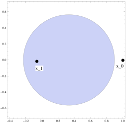
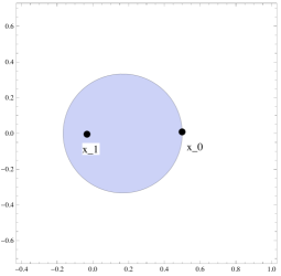
Figure 2. The case $p=\lambda=2$. On the left $|x_{0}|=1$ gives $|A_{opt}|=1$; on the right $|x_{0}|=1/2$ gives $|A_{opt}|\simeq 0.35$.

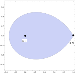
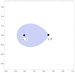
Figure 3. The case $p=1$ and $\lambda=2$. On the left $|x_{0}|=1$ gives $|A_{opt}|\simeq 0.97$; on the right $|x_{0}|=1/2$ gives $|A_{opt}|\simeq 0.24$.

7. Numerical simulations

For the numerical simulation of examples in the case of interpolation between measures (2.1) and the parking problem (6.2) we replace the optimal transportation costs by their entropically regularized versions. This will enable us to apply some variants of the celebrated Sinkhorn’s algorithm, popularized in the context of optimal transport and matching by [7] and [9]. For an introduction to this rapidly developing subject and convergence results, we refer the reader to [14] and [12].

7.1. Description of the Sinkhorn-like algorithm

The entropically regularized optimal transport cost for a cost function $c$, a regularizing parameter $\varepsilon>0$ and a fixed reference measure $Q\in\mathcal{P}(\mathbb{R}^{d}\times\mathbb{R}^{d})$ is given by

$$\inf\left\{\int_{\mathbb{R}^{d}\times\mathbb{R}^{d}}c(x,y)\,\,\mathrm{d}\gamma(x,y)+\varepsilon H(\gamma|Q)\;:\ \gamma\in\Pi(\mu_{0},\mu_{1})\right\},$$ (7.1)

where the relative entropy $H(P|Q)$ between two nonnegative finite measures $P,Q$ on $\mathbb{R}^{d}$ is defined by

$$H(P|Q)\coloneqq\begin{cases}\int_{\mathbb{R}^{d}}\left(\log\left(\frac{\,\mathrm{d}P}{\,\mathrm{d}Q}\right)-1\right)\,\mathrm{d}P\mbox{ if $P\ll Q$,}\\ +\infty\mbox{ otherwise.}\end{cases}$$

Note that, by setting $R=e^{-c/\varepsilon}Q$, we have

$$\varepsilon H(\gamma|R)=\int_{\mathbb{R}^{d}\times\mathbb{R}^{d}}c(x,y)\,\,\mathrm{d}\gamma(x,y)\ +\varepsilon H(\gamma|Q)$$

so that (7.1) amounts to minimizing $H(.|R)$ among transport plans between $\mu_{0}$ and $\mu_{1}$. As already observed in [2] in Section 3.2 the entropically regularized version of (2.1) becomes for two suitably chosen reference measures $R_{0}$, $R_{1}$

$$\inf\Big{\{}H(\gamma_{0}|R_{0})+H(\gamma_{1}|R_{1})\ :\ \mu\in\mathcal{A},\ \gamma_{0}\in\Pi(\mu_{0},\mu),\ \gamma_{1}\in\Pi(\mu,\mu_{1})\Big{\}}.$$ (7.2)

The cases i with no additional constraint and ii with location constraint $K$ can be treated by choosing the reference measures to enforce the support of $\mu$ being included in $K$. Namely we choose

$$R_{0}=e^{-c_{0}/\varepsilon}\mu_{0}\otimes\mathds{1}_{K},\quad R_{1}=e^{-c_{1}/\varepsilon}\mathds{1}_{K}\otimes\mu_{1},$$ (7.3)

where for case i we choose $K$ large enough (yet still compact) as before. The resulting Sinkhorn iterations are standard, see for instance Proposition 1 and 2 in [2]. The case iii of a density constraint $\phi$ requires performing a suitable projection of the estimated interpolation, as specified in Proposition 4.1 in [15] in the case of $\phi\equiv\kappa.$ We write the corresponding Sinkhorn iterations including the projection for the density constraint for sake of completeness in its dual form where the algorithm essentially becomes alternate gradient ascent. For this, note that the dual of (7.2) with $R_{i}$ as in (7.3) in the case of a density constraint $\mu\leq\phi$ ($\operatorname{spt}\phi\subset K$) is given by

$$\sup_{\begin{subarray}{c}\varphi_{0},\varphi_{1},\\ \psi_{0},\psi_{1}\end{subarray}}\left\{-\sum_{i=0}^{1}\int_{\mathbb{R}^{2d}}\exp\left(\varphi_{i}+\psi_{i}\right)\,\mathrm{d}R_{i}+\sum_{i=0}^{1}\int_{\mathbb{R}^{d}}\varphi_{i}\,\mathrm{d}\mu_{i}+\int_{\mathbb{R}^{d}}\left(\psi_{0}+\psi_{1}\right)\phi\,\mathrm{d}x:\psi_{0}+\psi_{1}\leq 0\right\}.$$

Sinkhorn iterations are given by the explicit coordinate ascent updates for this dual formulation:

$$\begin{split}&\exp\left(\varphi_{i}^{l+1}(x_{i})\right)=\left(\int_{K}\exp\left(-\frac{c_{i}}{\varepsilon}+\psi_{i}^{l}(x)\right)\,\mathrm{d}x\right)^{-1},\\ &\exp\left(\psi_{i}^{l+1}(x)\right)=\min\left\{\mu^{l},\phi\right\}\left(\int_{\mathbb{R}^{d}}\exp\left(-\frac{c_{i}}{\varepsilon}+\varphi_{i}^{l+1}(x_{i})\right)\,\mathrm{d}\mu_{i}(x_{i})\right)^{-1},\end{split}$$

where $\mu^{l}$ is the current approximate interpolation which is given by the geometric mean formula (see Proposition 2 of [2]):

$$\mu^{l}=\prod_{j=0}^{1}\left(\int\exp\left(-\frac{c_{j}}{\varepsilon}+\varphi_{j}^{l+1}+\psi_{j}^{l}\right)\,\mathrm{d}\mu_{j}(x_{j})\right)^{\frac{1}{2}}.$$

Regularizing the parking problem (6.2) in a similar way leads to

$$\inf_{\gamma,\tilde{\gamma_{0}},\tilde{\gamma_{1}},\tilde{\gamma}\in\mathcal{M}}\left\{H\left(\gamma|R\right)+H\left(\tilde{\gamma_{0}}|R_{0}\right)+H\left(\tilde{\gamma_{1}}|R_{1}\right)\right\},$$ (7.4)

where

$$\begin{split}\mathcal{M}&=\Big{\{}\gamma,\tilde{\gamma_{0}},\tilde{\gamma_{1}},\tilde{\gamma}\in\mathcal{M}_{+}(\mathbb{R}^{2d})^{3}\times\mathcal{M}_{+}(\mathbb{R}^{3d}):\\ &\qquad\gamma+\pi_{0,1}^{\#}\tilde{\gamma}\in\Pi(\nu_{0},\nu_{1}),\pi_{0,\mathrm{piv}}^{\#}\tilde{\gamma}=\tilde{\gamma_{0}},\pi_{\mathrm{piv},1}^{\#}\tilde{\gamma}=\tilde{\gamma_{1}}\Big{\}}.\end{split}$$

As before, a location constraint on a given set $K$ can be encoded in the choice of the reference measures:

$$R=e^{-c_{1}/\varepsilon}\nu_{0}\otimes\nu_{1},\quad R_{0}=e^{-c_{0}/\varepsilon}\nu_{0}\otimes\mathds{1}_{K},\quad R_{1}=e^{-c_{1}/\varepsilon}\mathds{1}_{K}\otimes\nu_{1}.$$

For the density constraint, we have to add the condition $\pi_{1}^{\#}\tilde{\gamma_{0}}\leq\phi$. The dual of (7.4) in the case of a density constraint is then given by

$$\sup_{\begin{subarray}{c}\varphi_{0},\varphi_{1},\\ \psi_{0},\psi_{1}\end{subarray}}\left\{-\int_{\mathbb{R}^{2d}}\exp\left(\varphi_{0}+\varphi_{1}\right)\,\mathrm{d}R-\sum_{i=0}^{1}\int_{\mathbb{R}^{2d}}\exp\left(\varphi_{i}+\psi_{i}\right)\,\mathrm{d}R_{i}\right.$$

$$\left.+\sum_{i=0}^{1}\int_{\mathbb{R}^{d}}\varphi_{i}\,\mathrm{d}\nu_{i}+\int_{\mathbb{R}^{d}}\left(\psi_{0}+\psi_{1}\right)\phi\,\mathrm{d}x\ :\ \psi_{0}+\psi_{1}\leq 0\right\}.$$

The Sinkhorn iterations (density constraint included) in the dual variables then become

$$\begin{split}\exp\left(\varphi_{i}^{l+1}(x_{i})\right)&=\left(\int\exp\left(-\frac{c_{1}}{\varepsilon}+\varphi_{i+1\mod 2}^{l}(x)\right)\,\mathrm{d}x+\int\exp\left(-\frac{c_{i}}{\varepsilon}+\psi_{i}^{l}(x)\right)\,\mathrm{d}x\right)^{-1},\\ \exp\left(\psi_{i}^{l+1}(x)\right)&=\min\left\{\mu^{l},\phi\right\}\left(\int\exp\left(-\frac{c_{i}}{\varepsilon}+\varphi_{i}^{l+1}(x_{i})\right)\,\mathrm{d}\mu_{i}(x_{i})\right)^{-1},\end{split}$$

and $\mu^{l}$, the current approximate parking measure, is again given by an explicit geometric mean expression.

7.2. Numerical results: comparison of the optimal interpolation and the optimal parking

We now present some numerical results based on the iterative schemes described in the previous paragraph. In all our examples (presented in Figures 4 to 7), we compare the solutions of the interpolation and parking problems with a constant density constraint on the unit square $K=[0,1]^{2}$. We always take as distribution of services $\mu_{1}=\nu_{1}=\delta_{(0.5,0.5)}$, the Dirac at the center of the square and as distribution of residents, we take a symmetric sum of four Dirac masses:

$$\mu_{0}=\nu_{0}=\frac{1}{4}\Big{(}\delta_{(0.5,0.1)}+\delta_{(0.5,0.9)}+\delta_{(0.1,0.5)}+\delta_{(0.9,0.5)}\Big{)}$$

We consider power-like costs

$$c_{0}(x,y)=|x-y|^{p},\qquad c_{1}(x,y)=1.5\,c_{0}(x,y)$$

for several values of $p$ corresponding to concave, linear or convex costs and various constant threshold values for the density constraints $\phi$. In this setting, we know (Corollary 3.3 for $p>1$ and Proposition 4.9 for $p\leq 1$) that the optimal interpolation and the optimal parking are of bang-bang type. Even with the entropic regularization (which has the effect of blurring the true solution) this is clearly what we observe in these figures with a small regularization $\varepsilon=5.10^{-4}$. Since the optimal parking may have total mass less than $1$ (it can even be $0$, see Figure 4), we have indicated its total mass on each figure, of course if the total mass of the parking is $1$ it coincides with the interpolation, a case which is more likely to occur when the threshold level is high. Finally, one can see the influence of the exponent $p$ on the shape of the support of the optimal measure and in particular recognize for $p=1$ (Figure 6) the drop-like shape which was explicitly computed and plotted in Figure 3 and balls for $p=2$ (Figure 7).

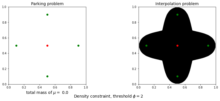
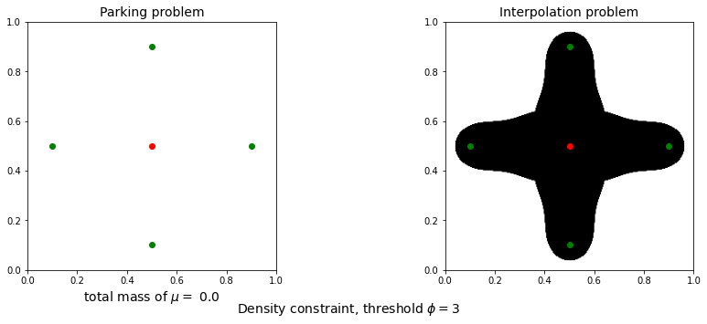
Figure 4. concave cost $p=0.25$

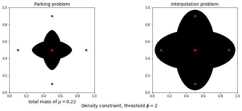
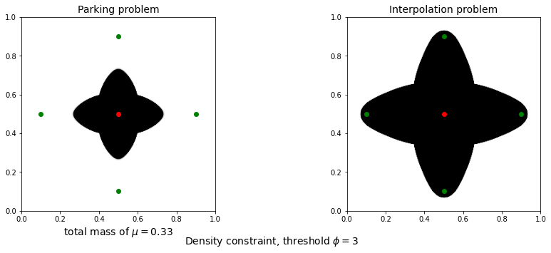
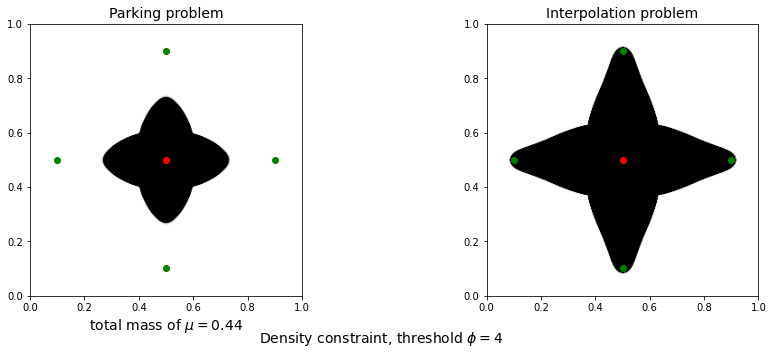
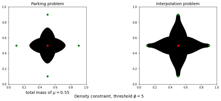
Figure 5. concave cost $p=0.75$

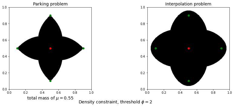
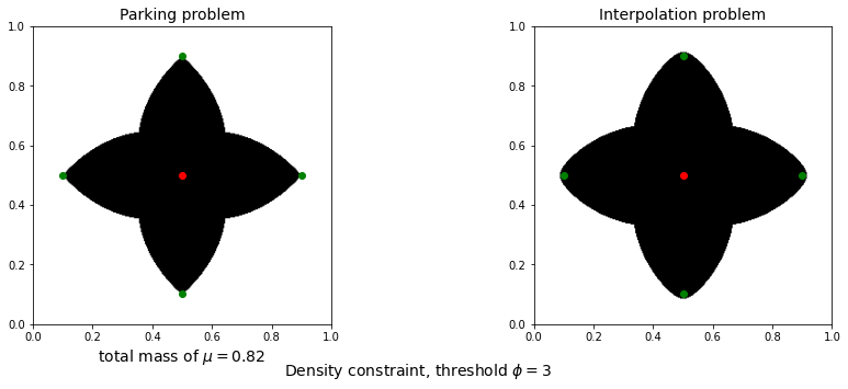
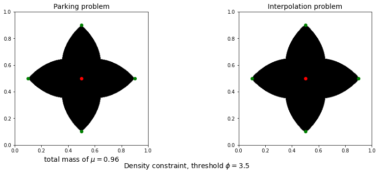
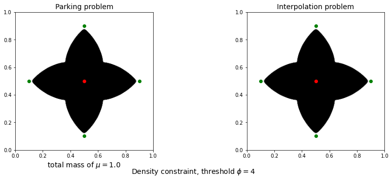
Figure 6. Linear cost $p=1$

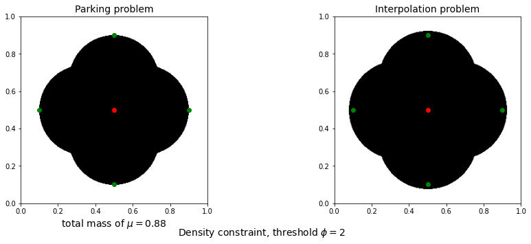
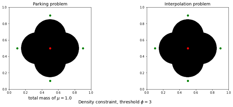
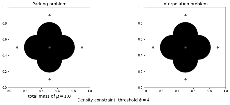
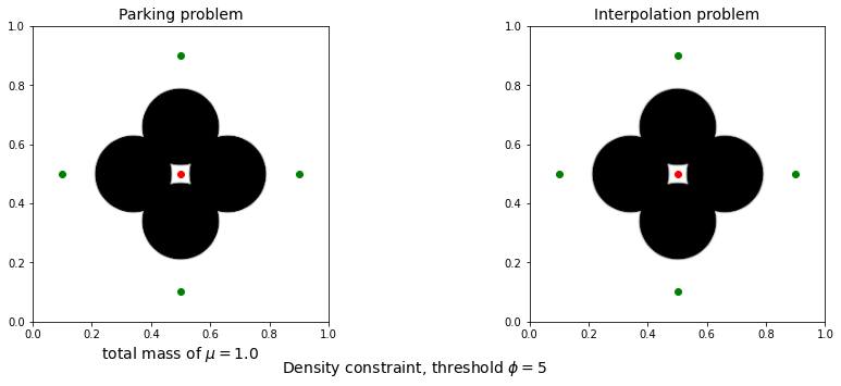
Figure 7. Convex cost $p=2$

Acknowledgments. The first author is member of the Gruppo Nazionale per l’Analisi Matematica, la Probabilità e le loro Applicazioni (GNAMPA) of the Istituto Nazionale di Alta Matematica (INdAM); his work is part of the project 2017TEXA3H “Gradient flows, Optimal Transport and Metric Measure Structures” funded by the Italian Ministry of Research and University. This work was initiated during a visit of GC and KE at the Dipartimento di Matematica of the University of Pisa, the hospitality of this institution is gratefully acknowledged as well as the support from the Agence Nationale de la Recherche through the project MAGA (ANR-16-CE40-0014). G.C. acknowledges the support of the Lagrange Mathematics and Computing Research Center. KE acknowledges that this project has received funding from the European Union’s Horizon 2020 research and innovation programme under the Marie Skłodowska-Curie grant agreement No 754362.

Giuseppe Buttazzo: Dipartimento di Matematica, Università di Pisa
Largo B. Pontecorvo 5, 56127 Pisa - ITALY
giuseppe.buttazzo@unipi.it
http://www.dm.unipi.it/pages/buttazzo/

Guillaume Carlier: CEREMADE, Université Paris Dauphine and Inria-Mokaplan, PSL
Place du Maréchal de Lattre de Tassigny, 75775 Paris Cedex 16 - FRANCE
carlier@ceremade.dauphine.fr
https://www.ceremade.dauphine.fr/ carlier/

Katharina Eichinger: CEREMADE, Université Paris Dauphine and Inria-Mokaplan, PSL
Place du Maréchal de Lattre de Tassigny, 75775 Paris Cedex 16 - FRANCE
eichinger@ceremade.dauphine.fr

References

• [1] Martial Agueh and Guillaume Carlier. Barycenters in the Wasserstein space. SIAM J. Math. Anal., 43(2):904โ€“924, 2011.
• [2] Jean-David Benamou, Guillaume Carlier, Marco Cuturi, Luca Nenna, and Gabriel Peyrรฉ. Iterative Bregman Projections for Regularized Transportation Problems. SIAM Journal on Scientific Computing, 37(2):A1111โ€“A1138, January 2015.
• [3] Giuseppe Buttazzo, Guillaume Carlier, and Maxime Laborde. On the Wasserstein distance between mutually singular measures. Adv. Calc. Var., 13(2):141โ€“154, 2020.
• [4] G.ย Carlier, E.ย Chenchene, and K.ย Eichinger. Wasserstein medians: theory and numerics. in preparation, 2022.
• [5] G.ย Carlier and I.ย Ekeland. Matching for teams. Econom. Theory, 42(2):397โ€“418, 2010.
• [6] Dario Cordero-Erausquin. Non-smooth differential properties of optimal transport. In Recent advances in the theory and applications of mass transport, volume 353 of Contemp. Math., pages 61โ€“71. Amer. Math. Soc., Providence, RI, 2004.
• [7] Marco Cuturi. Sinkhorn Distances: Lightspeed Computation of Optimal Transport. In Advances in Neural Information Processing Systems, volumeย 26. Curran Associates, Inc., 2013.
• [8] Lawrenceย C. Evans and Ronaldย F. Gariepy. Measure theory and fine properties of functions. Studies in Advanced Mathematics. CRC Press, Boca Raton, FL, 1992.
• [9] Alfred Galichon and Bernard Salaniรฉ. Matching with Trade-Offs: Revealed Preferences over Competing Characteristics. Technical Report info:hdl:2441/1293p84sf58s482v2dpn0gsd67, Sciences Po, March 2010. Publication Title: Sciences Po publications.
• [10] Wilfrid Gangbo and Robertย J. McCann. The geometry of optimal transportation. Acta Math., 177(2):113โ€“161, 1996.
• [11] Robertย J. McCann. A convexity principle for interacting gases. Adv. Math., 128(1):153โ€“179, 1997.
• [12] Marcel Nutz. Introduction to Entropic Optimal Transport, 2022.
• [13] Brendan Pass. Multi-marginal optimal transport and multi-agent matching problems: uniqueness and structure of solutions. Discrete Contin. Dyn. Syst., 34(4):1623โ€“1639, 2014.
• [14] Gabriel Peyrรฉ and Marco Cuturi. Computational Optimal Transport: With Applications to Data Science, volumeย 11. February 2019. Publisher: Now Publishers, Inc.
• [15] Gabriel Peyrรฉ. Entropic Approximation of Wasserstein Gradient Flows. SIAM Journal on Imaging Sciences, 8(4):2323โ€“2351, January 2015. Publisher: Society for Industrial and Applied Mathematics.
• [16] Davide Piazzoli, Filippo Santambrogio, and Paul Pegon. Full characterization of optimal transport plans for concave costs. Discrete and Continuous Dynamical Systems, 35(12):6113โ€“6132, May 2015.
• [17] Filippo Santambrogio. Optimal transport for applied mathematicians, volumeย 87 of Progress in Nonlinear Differential Equations and their Applications. Birkhรคuser/Springer, Cham, 2015. Calculus of variations, PDEs, and modeling.
• [18] Cรฉdric Villani. Topics in optimal transportation, volumeย 58 of Graduate Studies in Mathematics. American Mathematical Society, Providence, RI, 2003.