Complete three-loop QCD corrections to leptonic width of vector quarkonium

Abstract

Within the nonrelativistic QCD (NRQCD) factorization framework, we compute the order-$\alpha_{s}^{3}$ perturbative corrections to the leptonic decay of the $\Upsilon$ and $J/\psi$ with high numerical accuracy, at the lowest order in velocity expansion. We confirm the existing three-loop results in literature. Furthermore, we explicitly consider the complex-valued light-by-light (singlet) contributions. We for the first time also consider the finite charm quark mass effect for $\Upsilon$ leptonic decay, and obtain a new piece of 3-loop contribution to the anomalous dimension related to the composite NRQCD bilinear of vector current that arises from the nonzero charm quark mass. Based on the complete three-loop NRQCD short-distance coefficients, we also present a comprehensive phenomenological analysis for $\Upsilon(J/\psi)$ leptonic width.

I Introduction

The leptonic decay of vector quarkonium (exemplified by $J/\psi,\Upsilon\to l^{+}l^{-}$), as the simplest quarkonium decay process, has already been extensively studied both experimentally and theoretically. On the experimental side, these very clean decay channels have already been measured with very high precision. These decay channels are also very useful to reconstruct the vector quarkonium in various collision experiments. On the theoretically ground, these types of quarkonium electromagnetic decay processes directly probe the vector quarkonium decay constant, a basic nonperturbative parameter characterizing the quarkonium dynamics. Numerous theoretical efforts have been devoted to predicting the quakonium decay constant, including all sorts of phenomenological model predictions together with the first-principle approach, the lattice QCD simulation Hatton:2020qhk ; Hatton:2021dvg . Reassuringly, the good agreement is reached between the experimental measurement and lattice result.

From the theoretical angle, nonrelativistic QCD (NRQCD) Caswell:1985ui ; Bodwin:1994jh also provides a model-indepent framework to investigate the vector quarkonium leptonic decay. Since the leading-order (LO) prediction has been known since $1967$ VanRoyen:1967nq , a tremendous progress including higher-order corrections within the NRQCD framework has been constantly made during the past half century. For example, the $\mathcal{O}(\alpha_{s}v^{0})$ correction was computed in late 70s Barbieri:1975ki ; Celmaster:1978yz ($v$ denotes the typical heavy quark velocity inside quarkonium), while the leading relativistic correction of $\mathcal{O}(\alpha_{s}^{0}v^{2})$ and $\mathcal{O}(\alpha_{s}^{0}v^{4})$ were investigated in Bodwin:1994jh ; Bodwin:2002cfe . The $\mathcal{O}(\alpha_{s}v^{2})$ correction is calculated in Luke:1997ys . The two-loop QCD corrections yet at lowest order in $v$ were calculated in Czarnecki:1997vz ; Beneke:1997jm ; Kniehl:2006qw ; Egner:2021lxd . Finally, the $\mathcal{O}(\alpha_{s}^{3})$ fermionic Marquard:2006qi ; Marquard:2009bj and and pure gluonic corrections Marquard:2014pea ; Beneke:2014qea to $\Upsilon\to l^{+}l^{-}$ have also been known in the past decade.

In this paper, we make some further progress for the three-loop matching of the vector current into QCD with the corresponding operator in NRQCD. Explicitly speaking, we refine the existing three-loop results by including the light-by-light (singlet) contributions, as well as including the finite charm mass effect in $\Upsilon$ decay. There are some nontrivial technical challenges we have to overcome, because we have to deal with complex-valued loop integrals for the former, and deal with two mass scales in loop integration for the latter. Our calculation is made possible with the aid of the newly developed auxiliary mass flow (AMF) method to compute the master integrals with exceptional numerical accuracy Liu:2017jxz ; Liu:2020kpc ; Liu:2022chg . An interesting theoretical progress is that we find that the finite charm mass effect leads to a new piece of contribution to the three-loop anomalous dimension for the NRQCD vector current. We also present a comprehensive analysis of the $J/\psi$ and $\Upsilon$ leptonic decay width at the three-loop level, carefully assessing various sources of theoretical uncertainty.

The rest of the paper is structured as follows. In Section II, we recapitulate the general formalism for NRQCD factorization and vector current matching. In Section III we sketch the strategy of our three-loop calculation and present the numerical SDCs as well as the analytical expressions of the renormalization constant and the anomalous dimension of the NRQCD vector current. Section IV is devoted to phenomenological analysis of the confrontation of the finest NRQCD predictions to the measured $J/\psi$ and $\Upsilon$ leptonic decay width. Finally, we summarize Section V.

II Matching of the electromagnetic current

We start by define the leptonic decay constant $f_{V}$ for a given vector quarkonium $V$, through the vacuum-to-quarkonium matrix element of the electromagnetic current $\mathcal{J}_{\text{EM}}^{\mu}$:

$$\left\langle 0|\mathcal{J}_{\text{EM}}^{\mu}|V(\bm{\upepsilon})\right\rangle={M_{V}f_{V}\varepsilon_{V}^{\mu}},$$

$$\mathcal{J}_{\text{EM}}^{\mu}=\sum_{f}e_{f}\bar{\Psi}_{f}\gamma^{\mu}\Psi_{f},$$ (1)

where $M_{V}$ and $\varepsilon_{V}^{\mu}$ denote the mass and polarization vector of a vector quarkonium. The summation in definition of the EM current includes all the flavors of quarks, with $e_{u}=2/3$ for the up-type quarks and $e_{d}=-1/3$ for down-type quarks.

The leptonic decay width of the vector quarkonium $V$ then becomes

$$\Gamma(V\rightarrow l^{+}l^{-})={\dfrac{4\uppi\alpha^{2}}{3M_{V}}|f_{V}|^{2}},$$ (2)

where $\alpha$ is the QED fine structure constant.

According to NRQCD factorization formula, the decay constant $f_{V}$ is not a completely nonperturvative object. At the lowest order in velocity expansion, it can be further factorized in the following form:

$$f_{V}\epsilon_{V}^{i}= {\sqrt{2M_{V}}e_{Q}\mathcal{C}\dfrac{\left\langle 0|\tilde{j}^{i}|V(\bm{\upepsilon})\right\rangle}{M_{V}}}+\mathcal{O}\left(v^{2}\right)$$

$$= {\sqrt{2M_{V}}e_{Q}\left(\mathcal{C}_{\text{dir}}+\sum_{f\neq Q}\mathcal{C}_{\text{ind,f}}\dfrac{e_{f}}{e_{Q}}\right)\dfrac{\left\langle 0|\tilde{j}^{i}|V(\bm{\upepsilon})\right\rangle}{M_{V}}}+\mathcal{O}\left(v^{2}\right),$$ (3)

where $\tilde{j}=\chi^{\dagger}\bm{\upsigma}\psi$ is the corresponding NRQCD vector currentoperator, with $\sigma^{i}$ ($i=1,2,3$) denoting the Pauli matrices, and $\psi$ and $\chi^{\dagger}$ representing two-component spinor fields that annihilate a heavy quark and a heavy anti-quark, respectively. The factor $\sqrt{2M_{V}}$ has been explicitly inserted in the right-hand side of (3), in order to compensate the fact that the quarkonium state in the QCD side is relativistically normalized, where the quarkonium state in the NRQCD matrix element is conventionally nonrelativistically normalized. The dimensionless coefficient $\mathcal{C}$ is the short-distance coefficient (SDC), which encodes the effect from the relativistic quantum fluctuation, which can be reliably computed in perturbation theory owing to asymptotic freedom of QCD. For the sake of clarity, we devide the SDCs into two categories, the direct one and the indirect one. The former corresponds to the matching of heavy-quark vector current $j^{\mu}=\bar{\Psi}_{Q}\gamma^{\mu}\Psi_{Q}$ (the quark flavor in the current is the same as with the leading Fock state of a vector quarkonium). The latter arises from the contribution from the the quark flavors in the EM current in (1) which differ from the dominant quark flavor comprising the vector quarkonium. This can be viewed as the the manifestation of high-order Fock state components of a vector quarkonium with a short-distance origin. For example, the $\Upsilon$ may contain a tiny yet nonzero content of $u\bar{u}({}^{3}S_{1})$ or $c\bar{c}({}^{3}S_{1})$ components, since $b\bar{b}({}^{3}S_{1})$ might mix with these states through three-gluon annihilation.

The SDC can be systematically computed in perturbation theory since $m_{Q}\gg\Lambda_{\text{QCD}}$. The main purpose of this paper is to complete the evaluation of SDCs through ${\cal O}(\alpha_{s}^{3})$, , include the indirect contributions (often referred to as singlet or light-by-light contribution) and include the diagrams where the quarks in the closed loop can carry nonvanishing mass $m_{M}\neq m_{Q}$.

The SDC can be determined through the standard perturbative matching procedure. One calculates the on-shell vertex functions in both perturbative QCD and perturbative NRQCD sides, then solve the SDC through the following matching condition:

$$Z_{2}\Gamma= {\sqrt{2M_{V}}}\mathcal{C}\tilde{Z}_{2}\tilde{Z}_{v}^{-1}\tilde{\Gamma}+\mathcal{O}\left(v^{2}\right),$$ (4)

where the quantities with a tilde are defined in NRQCD. $Z_{2}$ denotes the on-shell field strength renormalization constant of the heavy quark. $\Gamma$ denotes the one-particle irreducible vertex diagrams with on-shell heavy quarks. Some representative diagrams up to two-loop order are shown in FIG. 1.

(a) LO

(b) NLO

(c) NNLO

Figure 1: Some representative Feynman diagrams up to two-loop order. The cross denotes the insertion of the external EM current.

${Z}_{v}=1$ since the vector current in QCD is a conserving current which does not require operator renormalization. $\tilde{Z}_{v}^{-1}$ is the renormalization constant affiliated with the NRQCD vector current $\tilde{\mathbf{j}}$. As for $\tilde{Z}_{v}$, the known analytical results only include the contributions of internal closed quark loops which are either massless or have the same mass with the external quark ($m_{Q}$) Beneke:1997jm ; Marquard:2006qi ; Kniehl:2002yv ; Beneke:2007pj . If we extend to the case where the closed quark loop could have a different mass ($m_{M}$), it is possible that $\tilde{Z}_{v}$ might contain an extra unknown term denoted as $\gamma_{0}$:

$$\tilde{Z}_{v}= 1+\left(\dfrac{\alpha_{s}(\mu_{\Lambda})}{\uppi}\right)^{2}\dfrac{C_{F}\uppi^{2}}{\epsilon}\left(\dfrac{1}{12}C_{F}+\dfrac{1}{8}C_{A}\right)+\left(\dfrac{\alpha_{s}(\mu_{\Lambda})}{\uppi}\right)^{3}C_{F}\uppi^{2}$$

$$\times\Bigg{\{}C_{F}^{2}\left[\dfrac{5}{144\epsilon^{2}}+\left(\dfrac{43}{144}-\dfrac{1}{2}\ln 2+\dfrac{5}{48}\ln\dfrac{\mu_{\Lambda}^{2}}{m_{Q}^{2}}\right)\dfrac{1}{\epsilon}\right]$$

$$+C_{F}C_{A}\left[\dfrac{1}{864\epsilon^{2}}+\left(\dfrac{113}{324}+\dfrac{1}{4}\ln 2+\dfrac{5}{32}\ln\dfrac{\mu_{\Lambda}^{2}}{m_{Q}^{2}}\right)\dfrac{1}{\epsilon}\right]$$

$$+C_{A}^{2}\left[-\dfrac{1}{16\epsilon^{2}}+\left(\dfrac{2}{27}+\dfrac{1}{4}\ln 2+\dfrac{1}{24}\ln\dfrac{\mu_{\Lambda}^{2}}{m_{Q}^{2}}\right)\dfrac{1}{\epsilon}\right]$$

$$+T_{F}n_{L}\left[C_{F}\left(\dfrac{1}{54\epsilon^{2}}-\dfrac{25}{324\epsilon}\right)+C_{A}\left(\dfrac{1}{36\epsilon^{2}}-\dfrac{37}{432\epsilon}\right)\right]$$

$$+T_{F}n_{H}\dfrac{C_{F}}{60\epsilon}+T_{F}n_{M}\dfrac{1}{\epsilon}\left[\gamma_{0}-\left(\dfrac{C_{F}}{18}+\dfrac{C_{A}}{12}\right){\ln\dfrac{\mu_{\Lambda}^{2}}{m_{Q}^{2}}}\right]\Bigg{\}}+{\cal O}\left(\alpha_{s}^{4}\right),$$ (5)

where $\mu_{\Lambda}$ is the NRQCD factorization scale, whose maximum value is around the heavy quark mass, the natural UV cutoff of NRQCD. The group-theoretical factors are $T_{F}=1/2,C_{F}=(N_{c}^{2}-1)/(2N_{c})$, $C_{A}=N_{c}$ relevant for $SU(N_{c})$. $n_{L}=3$ is the number of light quark flavours, $n_{H}=1$ is the number of heavy quark. Here we introduce $n_{M}$ indicating that the number of massive quark appearing the closed quark loop. For example, we choose $n_{M}=0$ in $J/\psi$ leptonic decay, but choose $n_{M}=1$ for $\Upsilon$ leptonic decay if we include the closed loop formed by the massive charm quark. Note that the strong coupling constant in this paper is defined in the effective theory of QCD with $n_{f}=n_{L}+n_{M}$ active quark flavors unless otherwise specified. $\tilde{Z}_{v}$ should return to the known single-mass-scale results with $n_{H}=2$ for $n_{M}=n_{H}$, i.e., $\gamma_{0}(m_{M}=m_{Q})=C_{F}/60$ Marquard:2014pea .

To expedite the matching procedure, we take the shortcut by neglecting the relative motion between the external heavy quark and heavy antiquark when computing the vertex function $\Gamma$. This amounts to applying the strategy of region Beneke:1997zp to directly extract the hard region contributions. It saves lots of labors since there is no need to evaluate any loop diagrams in the NRQCD side. As a consequence, one can simply set $\tilde{\Gamma}=1$ and $\tilde{Z}_{2}=1$ in (4).

At the $\text{N}^{3}$LO in $\alpha_{s}$, the dimensionless SDCs are expected to bear the following structure:

$$\mathcal{C}\left(\dfrac{\mu_{R}}{m_{Q}},\dfrac{\mu_{\Lambda}}{m_{Q}},x\right)= 1+\dfrac{\alpha_{s}\left(\mu_{R}\right)}{\uppi}\mathcal{C}^{\left(1\right)}+\left[\dfrac{\alpha_{s}\left(\mu_{R}\right)}{\uppi}\right]^{2}\left[\mathcal{C}^{\left(1\right)}\dfrac{\beta_{0}}{4}\ln\dfrac{\mu_{R}^{2}}{m_{Q}^{2}}+\gamma_{v}^{\left(2\right)}\ln\dfrac{\mu_{\Lambda}^{2}}{m_{Q}^{2}}+\mathcal{C}^{\left(2\right)}\left(x\right)\right]$$

$$+\left[\dfrac{\alpha_{s}\left(\mu_{R}\right)}{\uppi}\right]^{3}\Bigg{\{}\dfrac{\mathcal{C}^{\left(1\right)}}{16}\beta_{0}^{2}\ln^{2}\dfrac{\mu_{R}^{2}}{m_{Q}^{2}}+\left[\dfrac{\mathcal{C}^{\left(1\right)}}{16}\beta_{1}+\mathcal{C}^{\left(2\right)}\left(x\right)\dfrac{\beta_{0}}{2}\right]\ln\dfrac{\mu_{R}^{2}}{m_{Q}^{2}}$$

$$+\gamma_{v}^{\left(2\right)}\dfrac{\beta_{0}}{2}\ln\dfrac{\mu_{\Lambda}^{2}}{m_{Q}^{2}}\ln\dfrac{\mu_{R}^{2}}{m_{Q}^{2}}+\dfrac{1}{4}\left[2\dfrac{\mathrm{d}\gamma_{v}^{(3)}\left(\mu_{\Lambda}\right)}{\mathrm{d}\ln\mu_{\Lambda}^{2}}-\beta_{0}\gamma_{v}^{\left(2\right)}\right]\ln^{2}\dfrac{\mu_{\Lambda}^{2}}{m_{Q}^{2}}$$

$$+\left[\mathcal{C}^{\left(1\right)}\gamma_{v}^{\left(2\right)}+\gamma_{v}^{\left(3\right)}\left(m_{Q}\right)\right]\ln\dfrac{\mu_{\Lambda}^{2}}{m_{Q}^{2}}+\mathcal{C}^{\left(3\right)}\left(x\right)\Bigg{\}}+\mathcal{O}\left(\alpha_{s}^{4}\right),$$ (6)

where $\mu_{R}$ is the renormalization scale. $\beta_{0}=11C_{A}/3-4T_{F}n_{f}/3$ and $\beta_{1}=34C_{A}^{2}/3-20C_{A}T_{F}n_{f}/3-4C_{F}T_{F}n_{f}$ are the first two coefficients in the QCD $\beta$ function. Note $\mu_{R}$ has quite different physical origin from the NRQCD factorization scale $\mu_{\Lambda}$. The mass ratio is defined by

$$x=\dfrac{m_{M}}{m_{Q}}.$$ (7)

$\gamma_{v}^{\left(2\right)}$ and $\gamma_{v}^{\left(3\right)}$ are the various coefficients of the anomalous dimension associated with the NRQCD vector current $\tilde{\mathbf{j}}$, which can be deduced by taking the logarithmic derivative of the renormalization constant $\tilde{Z}_{v}$:

$$\gamma_{v}= \dfrac{\mathrm{d}\ln\tilde{Z}_{v}}{\mathrm{d}\ln\mu_{\Lambda}^{2}}=\left(\dfrac{\alpha_{s}}{\uppi}\right)^{2}\gamma_{v}^{(2)}+\left(\dfrac{\alpha_{s}}{\uppi}\right)^{3}\gamma_{v}^{(3)}{\left(\mu_{\Lambda}\right)}+\mathcal{O}\left(\alpha_{s}^{4}\right).$$ (8)

The one- and two-loop corrections to the SDCs have been known long ago Kallen:1955fb ; Czarnecki:1997vz ; Beneke:1997jm ; Kniehl:2006qw ; Egner:2021lxd :

$$\mathcal{C}^{(1)}= -2C_{F},$$

$$\mathcal{C}^{(2)}= \left[-\dfrac{151}{72}+\dfrac{89\uppi^{2}}{144}-\dfrac{5\uppi^{2}}{6}\ln 2-\dfrac{13}{4}\zeta(3)\right]C_{A}C_{F}+\left[\dfrac{23}{8}-\dfrac{79\uppi^{2}}{36}+\uppi^{2}\ln 2-\dfrac{1}{2}\zeta(3)\right]C_{F}^{2}$$

$$+\left(\dfrac{22}{9}-\dfrac{2\uppi^{2}}{9}\right)C_{F}T_{F}n_{H}+\dfrac{11}{18}C_{F}T_{F}n_{L}$$

$$+n_{M}C_{F}T_{F}\bigg{\{}\dfrac{71}{72}+\dfrac{35x^{2}}{24}+\uppi^{2}\left(\dfrac{3}{32x}-\dfrac{11x}{48}-\dfrac{17x^{3}}{32}+\dfrac{2x^{4}}{9}\right)+\dfrac{1}{24}\left(23+19x^{2}\right)H_{0}(x)$$

$$+\dfrac{4}{3}x^{4}H_{0}^{2}(x)+\left(\dfrac{3}{16x}-\dfrac{11x}{24}-\dfrac{17x^{3}}{16}+\dfrac{4x^{4}}{3}\right)\left[H_{0}(x)H_{1}(x)-H_{0,1}(x)\right]$$

$$+\left(\dfrac{3}{16x}-\dfrac{11x}{24}-\dfrac{17x^{3}}{16}-\dfrac{4x^{4}}{3}\right)H_{-1,0}(x)+{\dfrac{2}{3}\ln\dfrac{m_{Q}^{2}}{m_{M}^{2}}}\bigg{\}},$$ (9)

where $H_{*}(x)$ are harmonic polylogarithms (HPLs).

III The SDCs in three loop

The Feynman diagrams for $\Gamma$ are generated by the packages QGraf Nogueira:1991ex and FeynArts Hahn:2000kx . There are more than $300$ diagrams contributing to the vector current matching at $\text{N}^{3}$LO. As illustrated in (3), the amplitudes have been divided into two classes: the direct one and indirect one. Some representative diagrams for each class are shown in FIG. 2 and FIG. 3, respectively. The latter contains a specific topology where a closed quark loop is linked with three gluons and the current. This topology is often denoted by the “light-by-light” or singlet diagrams in literature. We note that the singlet amplitudes in the direct channel has also been considered in a very recent preprint that investigating the three-loop corrections to massive quark vector form factor Boughezal:2022nof .

(a) $C_{F}^{3}$

(b) $(C_{A}-2C_{F})^{2}C_{F}$

(c) $(C_{A}-2C_{F})C_{F}^{2}$

(d) $(C_{A}-2C_{F})(C_{A}-C_{F})C_{F}$

(e) $C_{A}(C_{A}-2C_{F})C_{F}$

(f) $C_{A}C_{F}^{2}$

(g) $C_{A}^{2}C_{F}$

(h) $(C_{A}-2C_{F})C_{F}$

(i) $C_{A}C_{F}$

(j) $C_{F}^{2}$

(k) $C_{F}$

(l) $(4B_{F}\pm C_{A})C_{F}$

Figure 2: Some representative diagrams for the direct channel. The color factor $B_{F}$ is defined as $\sum_{bc}d^{abc}d^{ebc}\equiv 4B_{F}\delta^{ae}$ and $B_{F}=(N_{c}^{2}-4)/(4N_{c})$ for the $SU(N_{c})$ group.

(a) $\left(4B_{F}+C_{A}\right)C_{F}$

(b) $\left(4B_{F}-C_{A}\right)C_{F}$

Figure 3: Some representative diagrams for the indirect channel.

Since the sum of electric charge of three light quarks vanishes, i.e., $\sum_{l=u,d,s}e_{l}=0$, ${\mathcal{C}}_{\text{ind},l}^{(3)}$ can be safely ignored. Following the notation of literature Marquard:2014pea , we further decompose $\mathcal{C}^{(3)}_{\text{dir}}$ with respect to different color structures:

$$\mathcal{C}_{\text{dir}}^{(3)}= C_{F}\big{[}C_{F}^{2}\mathcal{C}_{FFF}+C_{F}C_{A}\mathcal{C}_{FFA}+C_{A}^{2}\mathcal{C}_{FAA}$$

$$+T_{F}n_{L}\left(C_{F}\mathcal{C}_{FFL}+C_{A}\mathcal{C}_{FAL}+T_{F}n_{H}\mathcal{C}_{FHL}+T_{F}n_{M}\mathcal{C}_{FML}+T_{F}n_{L}\mathcal{C}_{FLL}\right)$$

$$+T_{F}n_{H}\left(C_{F}\mathcal{C}_{FFH}+C_{A}\mathcal{C}_{FAH}+T_{F}n_{H}\mathcal{C}_{FHH}+T_{F}n_{M}\mathcal{C}_{FHM}+B_{F}\mathcal{C}_{BFH}\right)$$

$$+T_{F}n_{M}\left(C_{F}\mathcal{C}_{FFM}+C_{A}\mathcal{C}_{FAM}+T_{F}n_{M}\mathcal{C}_{FMM}\right)\big{]}.$$ (10)

In extracting the SDCs, we have employed the covariant projector technique to project the amplitude with free $Q\bar{Q}$ pair onto the desired quantum number ${}3S_{1}^{(1)}$. The packages FeynCalc/FormLink Mertig:1990an ; Feng:2012tk are then utilized to deal with the trace over Dirac and $SU(N_{c})$ color matrices. There are about $300$ master integrals (MIs) for the amplitudes after the integration-by-parts (IBP) reduction with the aid of Apart Feng:2012iq and FIRE Smirnov:2014hma . The ‘light-by-light” amplitudes have imaginary parts, making the numerical evaluation of these MIs a painful challenge for traditional numerical methods such as sector decomposition Hepp:1966eg . We instead turn to the newly developed AMF package based on numerical differential equation technique, which can compute the multi-loop MIs to a very high precision in a very effective way Liu:2017jxz ; Liu:2020kpc ; Liu:2022chg .

III.1 Reconstructing the NRQCD Renormalization Constant

To remove the UV divergences, we incorporate the on-shell field and mass renormalization by taking the order-$\alpha_{s}^{3}$ expressions of $Z_{2}$ and $Z_{m}$ from Broadhurst:1991fy ; Melnikov:2000zc ; Marquard:2007uj . The strong coupling constant is renormalized to two-loop order under $\overline{\rm MS}$ scheme. After the renormalization procedure, the amplitude still contains uncancelled IR poles. These IR divergences appearing in the hard region in QCD amplitude is an indicator that the NRQCD current requires additional renormalization, which should be cancelled by the UV divergences in $\tilde{Z}_{v}$. Therefore, one can calculate the coefficients of the single poles with different values of the mass ratio $x$, then reconstruct $\gamma_{0}$ through numerical fitting recipe:

$$\gamma_{0}=\dfrac{C_{F}m_{Q}^{2}}{60m_{M}^{2}}+\left(\dfrac{C_{F}}{18}+\dfrac{C_{A}}{12}\right)\ln\dfrac{m_{M}^{2}}{m_{Q}^{2}}.$$ (11)

This completes our knowledge about the renormalization constant $\tilde{Z}_{v}$. We are then able to deduce the complete expression for the anomalous dimension up to three-loop:

$$\gamma_{v}^{(2)}= -3\uppi^{2}C_{F}\left(\dfrac{1}{18}C_{F}+\dfrac{1}{12}C_{A}\right),$$

$$\gamma_{v}^{(3)}\left(\mu_{\Lambda}\right)= -3\uppi^{2}C_{F}\bigg{\{}\left(\dfrac{43}{144}-\dfrac{1}{2}\ln 2\right)C_{F}^{2}+\left(\dfrac{113}{324}+\dfrac{1}{4}\ln 2\right)C_{F}C_{A}+\left(\dfrac{2}{27}+\dfrac{1}{4}\ln 2\right)C_{A}^{2}$$

$$+T_{F}n_{L}\left(-\dfrac{25}{324}C_{F}-\dfrac{37}{432}C_{A}\right)+\dfrac{1}{60}T_{F}n_{H}C_{F}$$

$$+T_{F}n_{M}\left[\dfrac{1}{60x^{2}}+\left(\dfrac{1}{18}C_{F}+\dfrac{1}{12}C_{A}\right)\ln x^{2}\right]+\ln\dfrac{\mu_{\Lambda}^{2}}{m_{Q}^{2}}\bigg{[}\dfrac{5}{48}C_{F}^{2}+\dfrac{5}{32}C_{F}C_{A}$$

$$+\dfrac{1}{24}C_{A}^{2}-T_{F}n_{M}\left(\dfrac{1}{12}C_{F}+\dfrac{1}{8}C_{A}\right)\bigg{]}\bigg{\}}.$$ (12)

The $n_{M}$-independent parts of SDCs are independent of the mass ratio $x$. These SDCs, except for $\mathcal{C}_{BFH}$ and ${\mathcal{C}}_{\text{ind},l}^{(3)}$, have been evaluated in Marquard:2006qi ; Marquard:2009bj ; Marquard:2014pea ; Egner:2022jot . $\mathcal{C}_{FHL}$, $\mathcal{C}_{FLL}$ and $\mathcal{C}_{FHH}$ are calculated analytically, while others are known numerically. Our numerical results confirm the known results, but with much higher precision:

$$\mathcal{C}_{FFF}= {36.49486245880592537633476189872792031664181},$$

$$\mathcal{C}_{FFA}= {-188.07784165988071390579994023278476450389105},$$

$$\mathcal{C}_{FAA}= {-97.734973269918386342345245004574098439887181},$$

$$\mathcal{C}_{FFL}= {46.691692905515132467558267641260536017779126774},$$

$$\mathcal{C}_{FAL}= {39.6237185545244190773420474220534775186981204767},$$

$$\mathcal{C}_{FHL}= {-0.270250439156502171732138691397778647923997721},$$

$$\mathcal{C}_{FLL}= {-2.46833645448237411637054187652486189658968386},$$

$$\mathcal{C}_{FFH}= {-0.8435622911595001453055093736419593585798252},$$

$$\mathcal{C}_{FAH}= {-0.1024741614929317408574835971993802120163106},$$

$$\mathcal{C}_{FHH}= {0.05123960751198372493493118588999641369844635617},$$

$$\mathcal{C}_{BFH}= {2.1155782679809064984368222219139443700443356}$$

$${+\mathrm{i}\,0.494212710700672040241218108020160381155220487)},$$

$${\mathcal{C}}_{\text{ind},l}^{(3)}= T_{F}B_{F}C_{F}(-0.945532642977386+{\mathrm{i}\,1.28500237447426)}.$$ (13)

Since the $n_{M}$-dependent terms in the SDCs vary with $x$, they are complicated functions of $x$ instead of constants. We have numerically evaluate these terms with many different values of $x$ and show their profiles in FIG. 4.

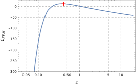
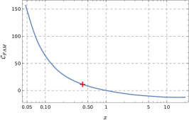
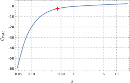
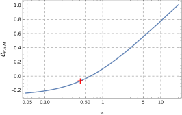
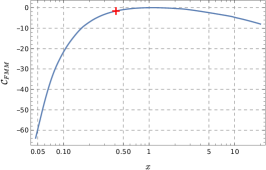
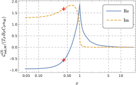
Figure 4: $n_{M}$-dependent terms of the SDCs as function of $x$. The crosses label the SDCs for $\Upsilon$ leptonic decay with charm quark mass $2.04$ GeV and bottom quark mass $4.98$ GeV. with physical mass ratio.

For reader’s convenience, we take the three-loop pole mass to be $m_{c}=2.04$ GeV and $m_{b}=4.98$ GeV, and define $x_{\text{phy}}$ as the corresponding ratio. We explicitly present the numerical SDCs for $\Upsilon$ decay with $x_{\text{phy}}=2.04/4.98$ as follows:

$$\mathcal{C}_{FFM}\left(x_{\text{phy}}\right)= 12.59634873592650205755866578463730117088523164,$$

$$\mathcal{C}_{FAM}\left(x_{\text{phy}}\right)= 11.485487450937888599629526907235667539099062,$$

$$\mathcal{C}_{FML}\left(x_{\text{phy}}\right)= -2.40343737830471435766973034309185481125317985382,$$

$$\mathcal{C}_{FHM}\left(x_{\text{phy}}\right)= -0.0697639123255824045909089712436335822048386627,$$

$$\mathcal{C}_{FMM}\left(x_{\text{phy}}\right)= -1.59441395438374277579099808902128228543581741117,$$

$${\mathcal{C}}_{\text{ind},M}^{(3)}\left(x_{\text{phy}}\right)= T_{F}B_{F}C_{F}n_{M}(-0.5600172596682562131259719921291458956964640$$

$${\mathrm{i}\,1.675430934114461038053844582307006798974491776)}.$$ (14)

We enumerate the SDCs at various perturbative order with $\mu_{R}=m_{b}$ and $\mu_{\Lambda}=1.5\,\mathrm{GeV}$. For the sake of clarity, we retain the explicit dependence on $n_{L},n_{H},n_{M}$ and separate out the “light-by-light” contributions at $\text{N}^{3}$LO:

$$\mathcal{C} \left({\mu_{R}=m_{b},\mu_{\Lambda}=1.5\,\mathrm{GeV},x_{\text{phy}}}\right)\approx 1-{\dfrac{8}{3}}\dfrac{\alpha_{s}(m_{b})}{\uppi}{-11.168625031474922}\left(\dfrac{\alpha_{s}(m_{b})}{\uppi}\right)^{2}$$

$$+\left(\dfrac{\alpha_{s}(m_{b})}{\uppi}\right)^{3}\big{[}{-1702.6786280810694238919125522+91.423820122192320694764194n_{L}}$$

$${+0.097945436227233777101707796n_{H}+19.1788305723128699826853781n_{M}}$$

$${-0.82277881816079137212351396n_{L}^{2}+0.0170798691706612416449770620n_{H}^{2}}$$

$${-0.53147131812791425859699936n_{M}^{2}-0.80114579276823811922324345n_{L}n_{M}}$$

$${-0.09008347971883405724404623n_{L}n_{H}-0.0232546374418608015303029904n_{M}n_{H}}$$

$$+(0.5876606299946962495657840+{\mathrm{i}\,0.1372813085279644556225606)_{\text{ind},H}}$$

$$+(0.3111206998156978961810956-{\mathrm{i}\,0.9307949633969227989188025)_{\text{ind},M}}\big{]}.$$ (15)

IV Phenomenology

With the complete three-loop SDCs in hand, we are able to present a finest NRQCD predictions to the leptonic width of vector quarkonium:

$$\Gamma(V\rightarrow l^{+}l^{-})={\dfrac{4\uppi\alpha^{2}}{3M_{V}}|f_{V}|^{2}}= \dfrac{8\uppi\alpha^{2}e_{Q}^{2}}{3M_{V}^{2}}\left|\mathcal{C}\left(\dfrac{\mu_{R}}{m_{Q}},\dfrac{\mu_{\Lambda}}{m_{Q}},x\right)\right|^{2}\left|\left\langle 0|\chi^{\dagger}\bm{\upsigma}\cdot\bm{\upepsilon}\psi(\mu_{\Lambda})|V(\bm{\upepsilon})\right\rangle\right|^{2}$$

$$= \dfrac{8\uppi\alpha^{2}e_{Q}^{2}}{3M_{V}^{2}}\left|\mathcal{C}_{\text{dir}}+\sum_{f\neq Q}\mathcal{C}_{\text{ind,f}}\dfrac{e_{f}}{e_{Q}}\right|^{2}\left|\left\langle 0|\chi^{\dagger}\bm{\upsigma}\cdot\bm{\upepsilon}\psi(\mu_{\Lambda})|V(\bm{\upepsilon})\right\rangle\right|^{2}.$$ (16)

The nonperturbative NRQCD matrix element can be estimated in variolous theoretical approach. It has been investigated in lattice NRQCD Choe:2003wx ; Gray:2005ur . In practice, it is often estimated in potential quark models and expressed in terms of $R_{V}(0)$, the radial Schrödinger function at the origin:

$$\left\langle 0|\chi^{\dagger}\bm{\upsigma}\cdot\bm{\upepsilon}\psi(\mu_{\Lambda})|V(\bm{\upepsilon})\right\rangle=\sqrt{\dfrac{N_{c}}{2\uppi}}R_{V}(0)$$ (17)

The exact value of $R_{V}(0)$ varies with the different potential models, which constitutes a major source of theoretical uncertainties. For reader’s convenience, in TABLE 1 we tabulate its value estimated in different potential models .

Potential Model	Cornell  Eichten:1995ch	Lattice  Choe:2003wx ; Gray:2005ur	B-T  Eichten:1995ch	Coul. $+$ power  Rai:2008sc	Bohr  Beneke:2014qea ; Egner:2021lxd	pNRQCD  Chung:2020zqc
$|R_{\Upsilon}(0)|^{2}\,(\mathrm{GeV}^{3})$	$14.05$	$5.05613$	$6.477$	$3.909\sim 9.181$	$2.1094^{+4.5371}_{-1.2913}$	$3.092$
$|R_{J/\psi}(0)|^{2}\,(\mathrm{GeV}^{3})$	$1.454$	$1.1184$	$0.810$	$0.610\sim 1.850$	$0.1423^{+0.5007}_{-0.0860}$	$0.421$
Potential Model	Screened  Azhothkaran:2020ipl	Power Law  Eichten:1995ch	Log  Eichten:1995ch	Modified NR  Akbar:2015evy ; Akbar:2011jd	Semi-relativistic  Radford:2007vd	Coul.
$|R_{\Upsilon}(0)|^{2}\,(\mathrm{GeV}^{3})$	$8.72$	$4.591$	$4.916$	$11.4185$	$6.143$	$4.221$
$|R_{J/\psi}(0)|^{2}\,(\mathrm{GeV}^{3})$	$1.19$	$0.999$	$0.815$	$1.9767$	$0.478$	$0.303$

Table 1: The values of $R_{V}(0)$ estimated in different theoretical approaches. Bowdin et al. Bodwin:2007fz also determined the value of LDMEs, and the results are not included here since their computation is based on the measured leptonic width as input.

In phenomenological study, we adopt the central value of $R_{V}(0)$ from the Buchmüller-Tye(BT) model Eichten:1995ch . To estimate the error caused by the uncertainty of the wave function at the origin, one may simply rescale the phenomenological predictions by a factor $\kappa$ to float the LDMEs. According to TABLE 1, one finds that $\kappa$ ranges from $0.1$ to $2.2$ for $\Upsilon$, and $0.07$ to $2.3$ for $J/\psi$.

To make concrete phenomenological predictions, we take the following values for various input parameters:

$${m_{b}=4.98\,\mathrm{GeV}},\quad{\alpha(2m_{b})=\dfrac{1}{132.5}},\quad\mu_{\Lambda}(\Upsilon)=1.5\,\mathrm{GeV},$$

$${m_{c}=2.04\,\mathrm{GeV}},\quad{\alpha(2m_{c})=\dfrac{1}{133.7}},\quad\mu_{\Lambda}(J/\psi)=1.0\,\mathrm{GeV}.$$ (18)

We compute the values bottom and charm quark pole mass using the three-loop formula by taking the precisely known $\overline{\text{MS}}$ masses as input. The running QED/QCD coupling constants $\alpha$/$\alpha_{s}$ are evaluated using the packages alphaQED Jegerlehner:2011mw and RunDec Herren:2017osy , respectively.

In TABLE 2, we present the NRQCD predictions at the various levels of perturbative accuracy for the leptonic width of $\Upsilon$ and $J/\psi$, juxtaposed with the precise experimental results. For $J/\psi$ decay, the bottom contributions are not included, i.e., $n_{M}=0$. The finite charm mass effect appears to be noticeable for the $\Upsilon$ leptonic decay, while the indirect contributions are completely insignificant. It seems that after including the $\text{N}^{3}$LO corrections, the finest NRQCD predictions for $\Upsilon$ and $J/\psi$ are much smaller than the experimental data.

In FIG. 5 we plot our NRQCD predictions for leptonic width as a function of $\mu_{R}$ at different levels of perturbative order. At $\text{N}^{3}$LO, the renormalization scale dependence becomes much worse than the lower orders. The reason is that the SDCs $\mathcal{C}_{FFA}$ and $\mathcal{C}_{FAA}$ are very large. In FIG. 6, we plot the $\text{N}^{3}$LO decay rate of $\Upsilon$ for both massive and massless charm cases.

	LO	NLO	NNLO	$\text{N}^{3}$LO			PDG
				Direct ($m_{M}=0$)	Direct ($m_{M}\neq 0$)	Total
$\Upsilon$	${1.6529}$	${{1.1095}_{-0.2922}^{+0.0888}}$	${{0.9750}_{-0.0942}^{+0.0642}}$	${0.1948_{-0.1948}^{+1.5900}}$	${{0.1763}_{-0.1763}^{+1.9577}}$	${{0.1764}_{-0.1764}^{+1.9560}}$	$1.340\pm 0.018$
$J/\psi$	${4.8392}$	${2.6999_{-1.0391}^{+0.4925}}$	${1.3138_{-1.1444}^{+0.7094}}$	${3.2219_{-3.2219}^{+123.4838}}$			$5.53\pm 0.10$

Table 2: Leptonic widths of $J/\psi$ and $\Upsilon$. The central values of predictions are obtained by setting $\mu_{R}=m_{Q}$, while the errors are estimated by varying $\mu_{R}$ from $\mu_{\Lambda}$ to $2m_{Q}$.

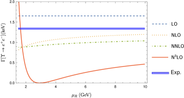
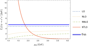
Figure 5: NRQCD predictions for leptonic width of $\Upsilon$ and $J/\psi$ as a function of renormalization scale $\mu_{R}$ at various level of perturbative expansion.

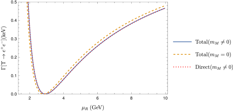
Figure 6: The $\text{N}^{3}$LO leptonic width of $\Upsilon$ as a function of renormalization scale $\mu_{R}$. One can see that the finite charm mass brings in a noticeable effect, but the indirect channel has a completely negligible impact.

V Summary

A complete $\text{N}^{3}$LO analysis of the $\Upsilon/J/\psi$ leptonic width is presented within the NRQCD factorization framework. The SDCs for both direct and indirect channels are calculated numerically with exquisitely high precision. We also consider the finite charm effect for $\Upsilon$ decay, also find a novel contribution to the anomalous dimension of NRQCD vector current for $\Upsilon$ decay that arises from keeping charm quark massive.

Adopting the values of the wave functions at the origin for $J/\psi$ and $\Upsilon$ from popular potential models, we evaluate the leptonic width of $\Upsilon$ and $J/\psi$ at $\text{N}^{3}$LO in $\alpha_{s}$. Unfortunately, the predictions exhibits a rather strong dependence on renormalization scale. For the natural range of $\mu_{R}$, there appears to exist an alarming discrepancy between the finest NRQCD predictions and the experimental data. How to resolve this discrepancy definitely deserves further investigation.

Appendix A $5$-Flavor

Our main results are expressed as a power series w.r.t. $\alpha_{s}^{(n_{L}+n_{M})}$ since the heavy quark is decoupled. In practice, we first calculate $\Gamma$ with $n_{L}+n_{M}+n_{H}$ active flavors in QCD and then apply the following formula to decouple the heavy quark from the running of $\alpha_{s}$.

$$\dfrac{\alpha_{s}^{\left(n_{L}+n_{M}+n_{H}\right)}\left(\mu_{R}\right)}{\pi}= \dfrac{\alpha_{s}^{\left(n_{L}+n_{M}\right)}\left(\mu_{R}\right)}{\pi}$$

$$+\left(\dfrac{\alpha_{s}^{\left(n_{L}+n_{M}\right)}\left(\mu_{R}\right)}{\pi}\right)^{2}T_{F}n_{H}\left[\dfrac{1}{3}\ln\dfrac{\mu_{\Lambda}^{2}}{m_{Q}^{2}}+\left(\dfrac{1}{6}\ln^{2}\dfrac{\mu_{\Lambda}}{m_{Q}}+\dfrac{1}{36}\pi^{2}\right)\epsilon+\mathcal{O}\left(\epsilon^{2}\right)\right]$$

$$+\left(\dfrac{\alpha_{s}^{\left(n_{L}+n_{M}\right)}\left(\mu_{R}\right)}{\pi}\right)^{3}T_{F}n_{H}\Bigg{[}\left(\dfrac{1}{4}\ln\dfrac{\mu_{\Lambda}^{2}}{m_{Q}^{2}}+\dfrac{15}{16}\right)C_{F}+\left(\dfrac{5}{12}\ln\dfrac{\mu_{\Lambda}^{2}}{m_{Q}^{2}}-\dfrac{2}{9}\right)C_{A}$$

$$+\dfrac{1}{9}T_{F}n_{H}\ln^{2}\dfrac{\mu_{\Lambda}}{m_{Q}}+\mathcal{O}\left(\epsilon\right)\Bigg{]}+{\cal O}\left(\alpha_{s}^{4}\right)$$ (19)

Here we also present the results with $n_{L}+n_{M}+n_{H}$ active flavors. To deal with the remaining IR divergence, one should adopt the corresponding renormalization constant with with $n_{L}+n_{M}+n_{H}$ active flavors. For simplicity, we omit the superscript $(n_{L}+n_{M}+n_{H})$ of $\alpha_{s}$ in the rest of paper.

$$\tilde{Z}_{v}= 1+\left(\dfrac{\alpha_{s}(\mu_{\Lambda})}{\uppi}\right)^{2}\dfrac{C_{F}\uppi^{2}}{\epsilon}\left(\dfrac{1}{12}C_{F}+\dfrac{1}{8}C_{A}\right)+\left(\dfrac{\alpha_{s}(\mu_{\Lambda})}{\uppi}\right)^{3}C_{F}\uppi^{2}$$

$$\times\Bigg{\{}C_{F}^{2}\left[\dfrac{5}{144\epsilon^{2}}+\left(\dfrac{43}{144}-\dfrac{1}{2}\ln 2+\dfrac{5}{48}\ln\dfrac{\mu_{\Lambda}^{2}}{m_{Q}^{2}}\right)\dfrac{1}{\epsilon}\right]$$

$$+C_{F}C_{A}\left[\dfrac{1}{864\epsilon^{2}}+\left(\dfrac{113}{324}+\dfrac{1}{4}\ln 2+\dfrac{5}{32}\ln\dfrac{\mu_{\Lambda}^{2}}{m_{Q}^{2}}\right)\dfrac{1}{\epsilon}\right]$$

$$+C_{A}^{2}\left[-\dfrac{1}{16\epsilon^{2}}+\left(\dfrac{2}{27}+\dfrac{1}{4}\ln 2+\dfrac{1}{24}\ln\dfrac{\mu_{\Lambda}^{2}}{m_{Q}^{2}}\right)\dfrac{1}{\epsilon}\right]$$

$$+T_{F}n_{L}\left[C_{F}\left(\dfrac{1}{54\epsilon^{2}}-\dfrac{25}{324\epsilon}\right)+C_{A}\left(\dfrac{1}{36\epsilon^{2}}-\dfrac{37}{432\epsilon}\right)\right]$$

$$+T_{F}n_{H}\left[\dfrac{C_{F}}{60\epsilon}-\left(\dfrac{1}{18}C_{F}+\dfrac{1}{12}C_{A}\right)\ln\dfrac{\mu_{\Lambda}^{2}}{m_{Q}^{2}}\dfrac{1}{\epsilon}\right]$$

$$+T_{F}n_{M}\left[\dfrac{1}{\epsilon}\gamma_{0}-\left(\dfrac{1}{18}C_{F}+\dfrac{1}{12}C_{A}\right)\ln\dfrac{\mu_{\Lambda}^{2}}{m_{Q}^{2}}\dfrac{1}{\epsilon}\right]\Bigg{\}}+{\cal O}(\alpha_{s}^{4})\,,$$ (20)

The SDCs are the same as the $n_{L}+n_{H}$-active-flavor case except for:

$$\mathcal{C}_{FFH}= {1.482405722886807434492825499916861}$$

$$\mathcal{C}_{FAH}= {0.129533415132085184395574268694405}$$ (21)

We plot the $\text{N}^{3}$LO NRQCD predictions for the decay rate as a function of $\mu_{R}$ with different active flavor numbers in FIG. 7. The $n_{L}+n_{M}+n_{H}$-active-flavor has a milder dependence on the renormalization scale.

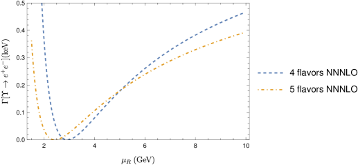
Figure 7: $\text{N}^{3}$LO NRQCD predictions for leptonic decay of $\Upsilon$ and $J/\psi$ as a function of renormalization scale $\mu_{R}$ with different active flavors.

References

- (1) D. Hatton et al. [HPQCD], Phys. Rev. D 102, no.5, 054511 (2020) doi:10.1103/PhysRevD.102.054511 [arXiv:2005.01845 [hep-lat]].
- (2) D. Hatton, C. T. H. Davies, J. Koponen, G. P. Lepage and A. T. Lytle, Phys. Rev. D 103, no.5, 054512 (2021) doi:10.1103/PhysRevD.103.054512 [arXiv:2101.08103 [hep-lat]].
- (3) W. E. Caswell and G. P. Lepage, Phys. Lett. B 167, 437-442 (1986) doi:10.1016/0370-2693(86)91297-9
- (4) G. T. Bodwin, E. Braaten and G. P. Lepage, Phys. Rev. D 51, 1125-1171 (1995) [erratum: Phys. Rev. D 55, 5853 (1997)] doi:10.1103/PhysRevD.55.5853 [arXiv:hep-ph/9407339 [hep-ph]].
- (5) R. Van Royen and V. F. Weisskopf, Nuovo Cim. A 50, 617-645 (1967) [erratum: Nuovo Cim. A 51, 583 (1967)] doi:10.1007/BF02823542
- (6) R. Barbieri, R. Gatto, R. Kogerler and Z. Kunszt, Phys. Lett. B 57, 455-459 (1975) doi:10.1016/0370-2693(75)90267-1
- (7) W. Celmaster, Phys. Rev. D 19, 1517 (1979) doi:10.1103/PhysRevD.19.1517
- (8) G. T. Bodwin and A. Petrelli, Phys. Rev. D 66, 094011 (2002) [erratum: Phys. Rev. D 87, no.3, 039902 (2013)] doi:10.1103/PhysRevD.66.094011 [arXiv:hep-ph/0205210 [hep-ph]].
- (9) M. E. Luke and M. J. Savage, Phys. Rev. D 57, 413-423 (1998) doi:10.1103/PhysRevD.57.413 [arXiv:hep-ph/9707313 [hep-ph]].
- (10) M. Beneke, A. Signer and V. A. Smirnov, Phys. Rev. Lett. 80, 2535-2538 (1998) doi:10.1103/PhysRevLett.80.2535 [arXiv:hep-ph/9712302 [hep-ph]].
- (11) A. Czarnecki and K. Melnikov, Phys. Rev. Lett. 80, 2531-2534 (1998) doi:10.1103/PhysRevLett.80.2531 [arXiv:hep-ph/9712222 [hep-ph]].
- (12) B. A. Kniehl, A. Onishchenko, J. H. Piclum and M. Steinhauser, Phys. Lett. B 638, 209-213 (2006) doi:10.1016/j.physletb.2006.05.023 [arXiv:hep-ph/0604072 [hep-ph]].
- (13) M. Egner, M. Fael, J. Piclum, K. Schoenwald and M. Steinhauser, Phys. Rev. D 104, no.5, 054033 (2021) doi:10.1103/PhysRevD.104.054033 [arXiv:2105.09332 [hep-ph]].
- (14) P. Marquard, J. H. Piclum, D. Seidel and M. Steinhauser, Nucl. Phys. B 758, 144-160 (2006) doi:10.1016/j.nuclphysb.2006.09.015 [arXiv:hep-ph/0607168 [hep-ph]].
- (15) P. Marquard, J. H. Piclum, D. Seidel and M. Steinhauser, Phys. Lett. B 678, 269-275 (2009) doi:10.1016/j.physletb.2009.05.070 [arXiv:0904.0920 [hep-ph]].
- (16) P. Marquard, J. H. Piclum, D. Seidel and M. Steinhauser, Phys. Rev. D 89, no.3, 034027 (2014) doi:10.1103/PhysRevD.89.034027 [arXiv:1401.3004 [hep-ph]].
- (17) M. Beneke, Y. Kiyo, P. Marquard, A. Penin, J. Piclum, D. Seidel and M. Steinhauser, Phys. Rev. Lett. 112, no.15, 151801 (2014) doi:10.1103/PhysRevLett.112.151801 [arXiv:1401.3005 [hep-ph]].
- (18) X. Liu, Y. Q. Ma and C. Y. Wang, Phys. Lett. B 779, 353-357 (2018) doi:10.1016/j.physletb.2018.02.026 [arXiv:1711.09572 [hep-ph]].
- (19) X. Liu, Y. Q. Ma, W. Tao and P. Zhang, Chin. Phys. C 45, no.1, 013115 (2021) doi:10.1088/1674-1137/abc538 [arXiv:2009.07987 [hep-ph]].
- (20) X. Liu and Y. Q. Ma, [arXiv:2201.11669 [hep-ph]].
- (21) M. Beneke, Y. Kiyo and A. A. Penin, Phys. Lett. B 653, 53-59 (2007) doi:10.1016/j.physletb.2007.06.068 [arXiv:0706.2733 [hep-ph]].
- (22) B. A. Kniehl, A. A. Penin, M. Steinhauser and V. A. Smirnov, Phys. Rev. Lett. 90, 212001 (2003) [erratum: Phys. Rev. Lett. 91, 139903 (2003)] doi:10.1103/PhysRevLett.90.212001 [arXiv:hep-ph/0210161 [hep-ph]].
- (23) M. Beneke and V. A. Smirnov, Nucl. Phys. B 522, 321-344 (1998) doi:10.1016/S0550-3213(98)00138-2 [arXiv:hep-ph/9711391 [hep-ph]].
- (24) A. O. G. Kallen and A. Sabry, Kong. Dan. Vid. Sel. Mat. Fys. Med. 29, no.17, 1-20 (1955) doi:10.1007/978-3-319-00627-7_93
- (25) P. Nogueira, J. Comput. Phys. 105, 279-289 (1993) doi:10.1006/jcph.1993.1074
- (26) T. Hahn, Comput. Phys. Commun. 140, 418-431 (2001) doi:10.1016/S0010-4655(01)00290-9 [arXiv:hep-ph/0012260 [hep-ph]].
- (27) R. Boughezal, Y. Huang and F. Petriello, [arXiv:2207.01703 [hep-ph]].
- (28) R. Mertig, M. Bohm and A. Denner, Comput. Phys. Commun. 64, 345-359 (1991) doi:10.1016/0010-4655(91)90130-D
- (29) F. Feng and R. Mertig, [arXiv:1212.3522 [hep-ph]].
- (30) F. Feng, Comput. Phys. Commun. 183, 2158-2164 (2012) doi:10.1016/j.cpc.2012.03.025 [arXiv:1204.2314 [hep-ph]].
- (31) A. V. Smirnov, Comput. Phys. Commun. 189, 182-191 (2015) doi:10.1016/j.cpc.2014.11.024 [arXiv:1408.2372 [hep-ph]].
- (32) K. Hepp, Commun. Math. Phys. 2, 301-326 (1966) doi:10.1007/BF01773358
- (33) D. J. Broadhurst, N. Gray and K. Schilcher, Z. Phys. C 52, 111-122 (1991) doi:10.1007/BF01412333
- (34) K. Melnikov and T. van Ritbergen, Nucl. Phys. B 591, 515-546 (2000) doi:10.1016/S0550-3213(00)00526-5 [arXiv:hep-ph/0005131 [hep-ph]].
- (35) P. Marquard, L. Mihaila, J. H. Piclum and M. Steinhauser, Nucl. Phys. B 773, 1-18 (2007) doi:10.1016/j.nuclphysb.2007.03.010 [arXiv:hep-ph/0702185 [hep-ph]].
- (36) M. Egner, M. Fael, F. Lange, K. Schönwald and M. Steinhauser, [arXiv:2203.11231 [hep-ph]].
- (37) S. Choe et al. [QCD-TARO], JHEP 08, 022 (2003) doi:10.1088/1126-6708/2003/08/022 [arXiv:hep-lat/0307004 [hep-lat]].
- (38) A. Gray, I. Allison, C. T. H. Davies, E. Dalgic, G. P. Lepage, J. Shigemitsu and M. Wingate, Phys. Rev. D 72, 094507 (2005) doi:10.1103/PhysRevD.72.094507 [arXiv:hep-lat/0507013 [hep-lat]].
- (39) E. J. Eichten and C. Quigg, Phys. Rev. D 52, 1726-1728 (1995) doi:10.1103/PhysRevD.52.1726 [arXiv:hep-ph/9503356 [hep-ph]].
- (40) A. K. Rai, B. Patel and P. C. Vinodkumar, Phys. Rev. C 78, 055202 (2008) doi:10.1103/PhysRevC.78.055202 [arXiv:0810.1832 [hep-ph]].
- (41) H. S. Chung, JHEP 12, 065 (2020) doi:10.1007/JHEP12(2020)065 [arXiv:2007.01737 [hep-ph]].
- (42) B. Azhothkaran and N. V. K., Int. J. Theor. Phys. 59, no.7, 2016-2028 (2020) doi:10.1007/s10773-020-04474-5
- (43) N. Akbar, M. A. Sultan, B. Masud and F. Akram, Phys. Rev. D 95, no.7, 074018 (2017) doi:10.1103/PhysRevD.95.074018 [arXiv:1511.03632 [hep-ph]].
- (44) N. Akbar, B. Masud and S. Noor, Eur. Phys. J. A 47, 124 (2011) [erratum: Eur. Phys. J. A 50, 121 (2014)] doi:10.1140/epja/i2011-11124-2 [arXiv:1106.3465 [hep-ph]].
- (45) S. F. Radford and W. W. Repko, Phys. Rev. D 75, 074031 (2007) doi:10.1103/PhysRevD.75.074031 [arXiv:hep-ph/0701117 [hep-ph]].
- (46) G. T. Bodwin, H. S. Chung, D. Kang, J. Lee and C. Yu, Phys. Rev. D 77, 094017 (2008) doi:10.1103/PhysRevD.77.094017 [arXiv:0710.0994 [hep-ph]].
- (47) F. Jegerlehner, Nuovo Cim. C 034S1, 31-40 (2011) doi:10.1393/ncc/i2011-11011-0 [arXiv:1107.4683 [hep-ph]].
- (48) F. Herren and M. Steinhauser, Comput. Phys. Commun. 224, 333-345 (2018) doi:10.1016/j.cpc.2017.11.014 [arXiv:1703.03751 [hep-ph]].