Abstract

Assuming confirmation of the anomalies in semi-leptonic $B$-decays, their explanation in terms of the exchange of a massive vector leptoquark field, $U_{\mu}^{a}$, of charge 2/3, appears to require the inclusion of $U_{\mu}^{a}$ in the vector multiplet of the adjoint of Pati-Salam $SU(4)$, $\mathcal{G}_{\mu}^{A}$, as well as the introduction of vector-like fermions, $F_{j}$, in the fundamental of $SU(4)$.

We consider simplified models characterised by the nature of the $SU(4)$ symmetry (global or local), by the number of vector-like fermions, and by the couplings of the Higgs boson to SM fermions (direct or induced by mixing with the vector-like fermions). In all cases, we implement a minimal breaking of a $U(2)^{n}_{f}$ flavour symmetry, with a single motivated exception. We then perform a global fit including the main observables sensitive to exchanges of the $\mathcal{G}_{\mu}^{A}$ at tree level and in loops dominated by logs insensitive to the UV completion.

1 Introduction and motivations

The intriguing deviations from the Standard Model (SM) appearing in neutral-current [1, 2, 3, 4] and charged-current [5, 6, 7, 8, 9, 10] semileptonic $B$-meson decays, if confirmed by experiments in progress, would point towards the existence of new physics close to the TeV scale, and hopefully shed some much-needed light on the flavour problem of the SM. This amply justifies the interest in the subject in the literature, with many different attempts put forward to explain these “B-anomalies”. Among them one emerging possibility is that the anomalies are due to the exchange of a vector leptoquark of charge $2/3$, $U_{\mu}^{a}$ [11] (see also Refs. [12, 13, 14]), for which several UV-complete models have been already suggested [15, 16, 17, 18, 19, 20, 21, 22].

Given this framework, generally speaking, two features seem unavoidable:

• The inclusion of $U_{\mu}^{a}$ in the vector multiplet, $\mathcal{G}_{\mu}^{A}$, of the adjoint of Pati-Salam $SU(4)$ with at least the first two generations of the Standard Model (SM) fermions not directly coupled to $\mathcal{G}_{\mu}^{A}$. Here we assume that at least some of the three generations of SM fermions, $f_{i}$, couple to the $\mathcal{G}_{\mu}^{A}$ by mixing with a suitable number of vector-like fermions, $F_{j}$, in the fundamental of $SU(4)$.

• An approximate flavour symmetry to allow for a relatively low mass for the vectors. To make contact with the observed pattern of quark and lepton masses and of quark mixings, we implement a minimal breaking of a $U(2)^{n}_{f}$ flavour symmetry, with a single motivated exception.

In this work, we propose a few simplified models that capture the essence of the vector leptoquark explanation of the anomalies and we analyse their consistency with the observables affected by $\mathcal{G}_{\mu}^{A}$ exchanges at tree level or in loops dominated by IR logs. While this is a seemingly step backward with respect to offering a full UV-complete model, we believe that this may help identify the proper direction for model building, as well as better appreciate the role of the expected experimental progress in different observables. To this end the tie with the observed flavour structure of the SM – which we shall implement differently in the different models – plays, in our view, a decisive role.

As said, we chose not to constrain ourselves into a specific UV-complete model. Nevertheless, broadly speaking, we have in mind at least two possibilities for the $\mathcal{G}_{\mu}^{A}$. They can be $\rho$-like states associated with a $SU(4)$ global symmetry of some strong dynamics at the TeV scale, with standard color $SU(3)$ gauged inside $SU(4)$ [15, 17]. Alternatively, $SU(4)$ can be part of a fully gauged $SU(4)\times SU(3)^{\prime}$, suitably included into a larger gauge group, with $SU(4)\times SU(3)^{\prime}$ broken to the diagonal standard colour $SU(3)$ [16, 18]. A model formulated in more than four dimensions can allow a bridge between these two scenarios [21, 23]. It is also conceivable, though not of concern in this work, that these models be extended to include as well a composite picture of ElectroWeak symmetry breaking, as in Refs. [17, 21, 22].

The paper is organised as follows. In Section 2 we define four different simplified models. In Section 3, for each model we determine the couplings of the massless fermions to the $\mathcal{G}_{\mu}^{A}$ before EW symmetry breaking, as well as their Yukawa couplings. Section 4 contains the phenomenological analysis. A discussion of the results is summarised in Section 5.

2 Definition of the models

A common element of the models we consider is a minimal set of $J$ vector-like fermions,

$$F_{j}=\left(\begin{array}[]{c}Q^{a}_{j}\\ L_{j}\end{array}\right)\,,\qquad j=1\dots J\,,$$ (2.1)

transforming in the fundamental of $SU(4)$. The apex $a$ is a color index, and $Q^{a}_{j}$ and $L_{j}$ are doublets under the standard $SU(2)_{L}$ gauge group, commuting with $SU(4)$. The $F_{j}$ have a universal mass term, $\mathcal{L}_{M}$, and a mass-mixing with the standard fermions $f_{i}$, $\mathcal{L}_{\rm mix}$:

$$\mathcal{L}_{m}=\mathcal{L}_{M}+\mathcal{L}_{\rm mix}\,,$$ (2.2)

and they may enter in the Yukawa couplings to the Higgs scalar in $\mathcal{L}_{Y}$. Both $\mathcal{L}_{m}$ and $\mathcal{L}_{Y}$ have to be invariant under the SM gauge group. The natural presence of further vector-like fermions in the fundamental of $SU(4)$ and transforming as singlets under $SU(2)_{L}$ does not play any significant phenomenological role, as we shall see in the following.

The four models that we consider (see Table 2.1) are classified according to the following properties:

• The coupling of the Higgs boson to the standard fermions $f_{i}$ is direct or arises only after their mixing with the vector-like fermions $F_{j}$;

• $SU(4)$ is a global or a local symmetry. In the latter case $SU(4)$ acts not only on the $F_{j}$ but also on the third family of standard quarks and leptons, extended to include a right-handed neutrino and organised in the usual Pati-Salam 4-plets.

In all cases, with a single motivated exception, we implement in both $\mathcal{L}_{Y}$ and $\mathcal{L}_{\rm mix}$ a minimal breaking of a $U(2)^{n}_{f}$ flavour symmetry acting on the first two generations of the $f_{i}$ [24, 25, 26] and, depending on the model, extended to the $F_{j}$.

Model	Direct SM Yukawa	$SU(4)$ gauged	min. $U(2)^{n}_{f}$ breaking	$J$
1	yes	no	yes	2
2	yes	yes	yes	1
3	yes	yes	no	2
4	no	no	yes	$3(\times 2)$

Table 2.1: Main features of the four simplified models considered.

2.1 Model 1

In this model, the SM fermions do not couple directly to the $\mathcal{G}_{\mu}^{A}$, while the two vector-like fermions $F_{j}$ are assumed to interact universally, in a $SU(4)$ invariant way, with the $\mathcal{G}_{\mu}^{A}$:

$$\mathcal{L}_{\rm int}=g_{U}\mathcal{G}_{\mu}^{A}J^{\mu\,A}\leavevmode\nobreak\ =\leavevmode\nobreak\ g_{U}\left[\frac{1}{\sqrt{2}}\left(U_{\mu}^{a}J_{U}^{\mu\,a}+{\rm h.c.}\right)+G^{\hat{a}}_{\mu}J_{G}^{\mu\,\hat{a}}+\frac{1}{2\sqrt{6}}\,X_{\mu}J_{X}^{\mu}\right]\,.$$ (2.3)

Here we have introduced, together with the leptoquark $U_{\mu}^{a}$, the coloron $G^{\hat{a}}_{\mu}$ and the $B$–$L$ vector $X_{\mu}$. The currents, written in terms of the components of the $F_{j}$, are

$${J}^{\mu\,a}_{U}\leavevmode\nobreak\ =\leavevmode\nobreak\ \bar{Q}_{j}^{a}\gamma_{\mu}L_{j}\,,\quad J_{G}^{\mu\,\hat{a}}\leavevmode\nobreak\ =\leavevmode\nobreak\ \bar{Q}_{j}T^{\hat{a}}\gamma_{\mu}Q_{j}\,,\quad{J}^{\mu}_{X}\leavevmode\nobreak\ =\leavevmode\nobreak\ \bar{Q}_{j}\gamma_{\mu}Q_{j}{-3}\bar{L}_{j}\,\gamma_{\mu}L_{j}\,.$$ (2.4)

with $j=1,2$. The flavour symmetry acting on the first two generations of chiral fermions $f_{i}$ is

$$U(2)^{5}_{f}=U(2)_{q}\times U(2)_{u}\times U(2)_{d}\times U(2)_{l}\times U(2)_{e},$$ (2.5)

where we used the standard notation for the irreducible representations of the SM gauge group. Following [24, 25, 26], we define as “minimal” the case where the breaking of $U(2)^{5}_{f}$ occurs only via

• the (leading) spurion doublets,

  $$V_{q}\sim 2_{q}\,,\qquad V_{l}\sim 2_{l}\,,$$ (2.6)

  whose natural size is set by the $32$ mixing in the CKM matrix ($|V_{cb}|\approx 4\times 10^{-2}$);

• the (subleading) spurion bi-doublets

  $$\Delta_{u}\sim(2_{q},\bar{2}_{u})\,,\quad\Delta_{d}\sim(2_{q},\bar{2}_{d})\,,\quad\Delta_{e}\sim(2_{l},\bar{2}_{e})\,,$$ (2.7)

  each with their two eigenvalues of order of magnitude similar to the two lightest quark and lepton masses relative to the third one.

The SM fermions couple directly to the Higgs field. The $U(2)^{5}_{f}$ breaking structure implies that the $3\times 3$ Yukawa matrices have the form

$$\mathcal{L}_{Y}^{u}=y_{t}H(\bar{q},\bar{q}_{3})\left(\begin{array}[]{c:c}\Delta_{u}&x_{t}V_{q}\\ \hdashline 0&1\end{array}\right)u_{R}\equiv H\bar{q}_{L}\hat{Y}_{u}u_{R}\,,$$ (2.8)

with $x_{t}={\mathcal{O}}(1)$, and similarly for $\mathcal{L}_{Y}^{d,e}$. After $SU(4)$ breaking, $\mathcal{L}_{m}=\mathcal{L}_{m}^{q}+\mathcal{L}_{m}^{l}$ can be decomposed as

$$\mathcal{L}_{m}^{q}=M[\bar{Q}_{j_{L}}+\alpha_{j}\bar{q}_{3}+\beta_{j}(\bar{q}V_{q})]Q_{j_{R}}\,,$$ (2.9)

with $\alpha_{j},\beta_{j}={\mathcal{O}}(1)$, and similarly for $\mathcal{L}_{m}^{l}$. In both Eq. (2.8) and Eq. (2.9) $V_{q}$ is contracted with the doublet component of $q$ under $U(2)_{q}$. Note that the minimality of the $U(2)^{5}_{f}$ breaking forbids any mixing of the two light generations with possible vector-like $SU(2)_{L}$-singlet fermions, thus justifying not having included the latter in the first place.

2.2 Model 2

At variance with Model 1, in Model 2 $SU(4)$ is gauged and acts also on the third family of SM quarks and leptons, embedded in Pati-Salam 4-plets with the addition of a right-handed neutrino. We also assume a single family of vector-like fermions charged under $SU(2)_{L}$ and $SU(4)$. The relevant part of the $SU(4)$ currents in Eq. (2.4) receives extra pieces:

$${J}^{\mu\,a}_{U}\leavevmode\nobreak\ =\leavevmode\nobreak\ \bar{Q}^{a}_{j}\gamma_{\mu}L_{j}+\bar{q}^{a}_{3}\gamma_{\mu}l_{3}\,,$$ (2.10)

$$J_{G}^{\mu\,\hat{a}}\leavevmode\nobreak\ =\leavevmode\nobreak\ \,\bar{Q}_{j}T^{\hat{a}}\gamma_{\mu}Q_{j}+\bar{q}_{3}T^{\hat{a}}\gamma_{\mu}q_{3}\,,$$ (2.11)

$${J}^{\mu}_{X}\leavevmode\nobreak\ =\leavevmode\nobreak\ \bar{Q}_{j}\gamma_{\mu}Q_{j}{-3}\bar{L}_{j}\,\gamma_{\mu}L_{j}+\bar{q}_{3}\gamma_{\mu}q_{3}{-3}\bar{l}_{3}\,\gamma_{\mu}l_{3}\,,$$ (2.12)

where we include explicitly only the left-handed $SU(2)_{L}$ doublets. We left the index $j$ for later purpose, although in this case there is a single family of vector-like fermions, dubbed $j=2$ for ease of notation. Unlike in Model 1, in this case, the universality of the couplings in these currents is dictated by gauge invariance.

The structure of both Yukawa coupling and vector-like mass terms is like in Model 1. Note, however, that in this case, we need $SU(4)$-breaking terms not only in $\mathcal{L}_{m}$ but also in the Yukawa coupling: the mixing between light and third generations in Eq. (2.8) breaks explicitly the $SU(4)$ gauge symmetry. This term can be viewed as the effective result of a $SU(4)$-conserving Yukawa interaction between vector-like fermions and the Higgs, after integrating out the heavy fermions.

2.3 Model 3

In Model 3 there is no change with respect to Model 2 either in the gauge structure or in the Yukawa couplings. However, we enlarge the matter field content with a second family of vector-like fermions ($j=1,2$). This allows us to extend the flavour symmetry to $U(2)^{5}_{f}\times U(2)_{F}$, and to introduce a non-minimal breaking of $U(2)^{5}_{f}$ via the bi-doublets

$$\Delta^{q}=(2_{q},\bar{2}_{F})\,,\qquad\Delta^{l}=(2_{l},\bar{2}_{F})\,.$$ (2.13)

The latter control the mixing between light families and vector-like fermions via

$$\mathcal{L}_{m}^{q}=M\left[\bar{Q}_{j_{L}}+\alpha_{j}\bar{q}_{3}+\bar{q}_{i}\Delta^{q}_{ij}\right]Q_{j_{R}}\,,$$ (2.14)

and similarly in $\mathcal{L}^{q}_{m}$. This will have important consequences for the alignment of the Yukawa couplings, which are not generic, with the mass eigenstates.

2.4 Model 4

As we are going to see, in none of the previous models there is a fixed orientation of the vector-like–SM-fermion mixing with respect to the up or down SM Yukawa couplings. This introduces an intrinsic uncertainty of the order of the Cabibbo-Kobayashi-Maskawa matrix, $V_{\rm CKM}$, in this relative orientation. To avoid this feature, we consider a model in which, as in Ref. [17], there is a doubling of the three vector-like $SU(4)$ multiplets (with the same weakly gauged quantum numbers)

$$F^{u}_{i}=(Q^{u},L^{\nu})_{i}\,,\quad F^{d}_{i}=(Q^{d},L^{e})_{i}\,,\quad\quad i=1,2,3\,,$$ (2.15)

and assume no direct coupling between the $SU(2)_{L}$-charged SM fermions and the Higgs. We further assume that:

• As in Model 1, only the vector-like fermions couple in a flavour universal way to the $\mathcal{G}_{\mu}^{A}$:

  $${J}^{\mu\,a}_{U}\leavevmode\nobreak\ =\leavevmode\nobreak\ \bar{Q}^{u\,a}_{i}\gamma_{\mu}L^{\nu}_{i}+\bar{Q}^{d\,a}_{i}\gamma_{\mu}L^{e}_{i}\,,$$ (2.16)

  $$J_{G}^{\mu\,\hat{a}}\leavevmode\nobreak\ =\leavevmode\nobreak\ \,\bar{Q}_{i}^{u}T^{\hat{a}}\gamma_{\mu}Q_{i}^{u}+\bar{Q}_{i}^{d}T^{\hat{a}}\gamma_{\mu}Q_{i}^{d}\,,$$ (2.17)

  $${J}^{\mu}_{X}\leavevmode\nobreak\ =\leavevmode\nobreak\ \bar{Q}_{i}^{u}\gamma_{\mu}Q_{i}^{u}+\bar{Q}_{i}^{d}\gamma_{\mu}Q_{i}^{d}{-3}\bar{L}_{i}^{\nu}\,\gamma_{\mu}L_{i}^{\nu}{-3}\bar{L}_{i}^{e}\,\gamma_{\mu}L_{i}^{e}\,.$$ (2.18)

• The allowed Yukawa couplings are between vector-like and chiral fermions,

  $$\mathcal{L}_{Y}=H\bar{Q}^{u}_{L}Y_{u}u_{R}+H\bar{L}^{\nu}_{L}Y_{\nu}\nu_{R}+H^{*}\bar{Q}^{d}_{L}Y_{d}d_{R}+H^{*}\bar{L}^{e}_{L}Y_{e}e_{R},$$ (2.19)

  and they are assumed to respect a product $U(2)_{F_{u}+u+\nu}\times U(2)_{F_{d}+d+e}$ of diagonal symmetries. The minimal breaking of the overall $U(2)_{q}\times U(2)_{l}\times U(2)_{F_{u}+u+\nu}\times U(2)_{F_{d}+d+e}$ flavour symmetry is controlled by

  $$\mathcal{L}_{\rm mix}=\bar{q}_{L}\hat{m}_{u}Q^{u}_{R}+\bar{q}_{L}\hat{m}_{d}Q^{d}_{R}+\bar{l}_{L}\hat{m}_{e}L^{e}_{R}+\bar{l}_{L}\hat{m}_{\nu}L^{\nu}_{R}\,,$$ (2.20)

  with the mixing matrices $\hat{m}_{u,d,e,\nu}$ having the same flavour structure as the Yukawa couplings in Eq. (2.8).

3 Couplings of the massless fermions

In this Section, we derive the couplings of the fermions which are massless before ElectroWeak symmetry breaking. Needless to say, their couplings to the SM gauge bosons are fixed by gauge invariance. We thus need to derive the couplings to the $\mathcal{G}_{\mu}^{A}$ and the Yukawa couplings, which are not flavour generic.

3.1 Model 1

Without loss of generality, we can take the spurion doublet $V_{q}$ oriented in the direction of $q_{2}$ with a single entry $\epsilon_{q}=O(|V_{cb}|)$. This way, the mixing part in Eq. (2.9) involves only the 2–3 sector and can be put in the form

$$\mathcal{L}_{\rm mix}=\bar{q}_{L}U_{q}m_{q}W_{q}^{+}Q_{R}\,,\qquad q_{L}=\left(\begin{array}[]{c}q_{2}\\ q_{3}\end{array}\right)\,,\quad Q_{R}=\left(\begin{array}[]{c}Q_{1_{R}}\\ Q_{2_{R}}\end{array}\right)\,,$$ (3.1)

where

$$m_{q}=M\left(\begin{array}[]{cc}O(\epsilon_{q})&0\\ 0&O(1)\end{array}\right),$$ (3.2)

and $U_{q}$ and $W_{q}$ are $2\times 2$ unitary matrices with off-diagonal elements of order $\epsilon_{q}$ and $1$, respectively. Note that, differently from the previous section, here $q_{L}$ denotes a two-component vector. We will go back to the three-family notation at the end of this section.

After inserting Eq. (3.1) into (2.9), the complete $\mathcal{L}_{m}$ leads to two massive states

$$Q^{h}_{L}=s_{q}U_{q}^{+}q_{L}+c_{q}W_{q}^{+}Q_{L}\,,\quad s_{q}=\frac{m_{q}}{\sqrt{m_{q}^{2}+M^{2}}}\,,$$ (3.3)

and two massless orthogonal combinations

$$q^{l}_{L}=c_{q}U_{q}^{+}q_{L}-s_{q}W_{q}^{+}Q_{L}\,,$$ (3.4)

which acquire a mass only via the Yukawa interaction. By inverting these equations, the components of the (interaction) fields $Q_{L}$ and $q_{L}$ involving the light states are

$$\left.Q_{L}\right|_{\rm light}=-W_{q}s_{q}q^{l}_{L}\,,\qquad\left.q_{L}\right|_{\rm light}=U_{q}c_{q}q^{l}_{L}\,.$$ (3.5)

Analogous expressions hold for the leptons.

The insertion of $Q_{L}|_{\rm light}$ and $L_{L}|_{\rm light}$ into the currents in Eq. (2.4) yields the couplings of the light states to the $SU(4)$ vectors. To simplify the notation we remove the suffix $l$ from the fields. For the coloron and the $B$–$L$ current there are no flavor-changing couplings:

$$J_{\mu}^{G\,\hat{a}} = \bar{q}_{L}s_{q}^{2}\gamma_{\mu}T^{\hat{a}}q_{L}\,,$$ (3.6)

$$J_{\mu}^{X} = \bar{q}_{L}s_{q}^{2}\gamma_{\mu}q_{L}-3\bar{l}_{L}s_{l}^{2}\gamma_{\mu}l_{L}\,.$$ (3.7)

The leptoquark current instead has the form:

$$J_{\mu}^{U\,a}=\bar{q}_{L}^{a}s_{q}Ws_{l}\gamma_{\mu}l_{L}\,,\quad\quad W=W_{q}^{+}W_{l}\,.$$ (3.8)

Since $q_{1}$ does not enter $\mathcal{L}_{\rm mix}$, we have $q_{1}=q_{1}^{l}$, hence in these expressions for the $SU(4)$ currents $q_{L}$ and $l_{L}$ can be thought to include all the three generations with $s_{q_{1}}=s_{l_{1}}=0$. Note that here the $q_{L}$ field does not correspond either to the up- or to the down-quark mass eigenstates, since we have not fully diagonalised the Yukawa couplings yet; similar considerations hold for $l_{L}$. It is readily seen that the transformation $q_{L}\rightarrow U_{q}c_{q}q^{l}$ in the 2–3 sector does not alter the structure of the Yukawa couplings in (2.8). These are diagonalised by a proper unitary matrix on the left side only.

$$\hat{y}_{d}=U_{d}y_{d}^{\rm diag}\,,\qquad\hat{y}_{u}=U_{u}y_{u}^{\rm diag}\,,\qquad\hat{y}_{e}=U_{e}y_{e}^{\rm diag}\,,$$ (3.9)

where $U_{u}=U_{d}V_{\rm CKM}^{\dagger}$. As shown in Ref. [27], $U_{d}$ and $U_{e}$ have the following parametric form:

$$U_{d}\approx\begin{pmatrix}c_{d}&-s_{d}\,e^{i\alpha_{d}}&0\\ s_{d}\,e^{-i\alpha_{d}}&c_{d}&s_{b}\\ -s_{d}\,s_{b}\,e^{-i(\alpha_{d}+\phi_{q})}&-c_{d}\,s_{b}\,e^{-i\phi_{q}}&e^{-i\phi_{q}}\end{pmatrix}\,,\qquad U_{e}\approx\begin{pmatrix}c_{e}&-s_{e}&0\\ s_{e}&c_{e}&s_{\tau}\\ -s_{e}s_{\tau}&-c_{e}s_{\tau}&1\end{pmatrix}\,.$$ (3.10)

These expressions are obtained expanding up to first non-trivial terms in the small mixing parameters $s_{d,b,e,\tau}$ with $s_{i}=\sin\theta_{i}$, $c_{i}=\cos\theta_{i}$. The known structure of the CKM matrix implies that $s_{d}$ and $\alpha_{d}$ are not free but are constrained by

$$\frac{s_{d}}{c_{d}}=\left|\frac{V_{td}}{V_{ts}}\right|\,,\qquad\alpha_{d}=\arg(V_{td}^{*}/V_{ts}^{*})\,.$$ (3.11)

On the other hand, the $2$–$3$ mixing angles, which are related to the Yukawa parameters by $s_{b}/c_{b}=|x_{b}|\,|V_{q}|$ and $s_{\tau}/c_{\tau}=|x_{\tau}|\,|V_{\ell}|$, cannot be expressed in terms of SM observables. Unconstrained are also $s_{e}$ and $\phi_{q}$ (that becomes unphysical in the limit $s_{b}\to 0$).

The $3\times 3$ unitary matrices $U_{d,u,e}$ appear in the currents (3.6)–(3.8) once these are written in terms of mass eigenstates. For instance, the coloron current involving down-type quarks takes the form

$$\left.J_{\mu}^{G\,\hat{a}}\right|_{\rm down}=\bar{d}_{L}\,U^{\dagger}_{d}s_{q}^{2}\gamma_{\mu}T^{\hat{a}}U_{d}\,q_{L}\,.$$ (3.12)

3.2 Models 2 and 3

We can effectively discuss these two models together by assuming two families of vector-like fermions and later treating $F_{1}$ as a null entry in Model 2. The part of $\mathcal{L}_{m}$ that contains only $SU(4)$ 4-plets $(f_{3},F_{1},F_{2})$ can be diagonalised by the unitary transformation

$$\left(\begin{matrix}q_{3}\\ Q_{1_{L}}\\ Q_{2_{L}}\end{matrix}\right)=W_{q}\left(\begin{matrix}q_{3}^{l}\\ Q_{1_{L}}^{h}\\ Q_{2_{L}}^{h}\end{matrix}\right)\,,$$ (3.13)

and similarly in the $2\times 2$ $Q_{R}$ sector. We can proceed analogously in the lepton sector.

In this new basis, the coloron and the $X$ currents remain universal and diagonal, whereas the leptoquark current is modified by a unitary matrix $W_{q}W_{l}^{+}\equiv W$. Also, mass mixing occurs only in the $2\times 2$ sector:

$$\mathcal{L}_{m}=M\bar{q}_{i}\tilde{\Delta}_{ij}Q_{j_{R}}^{h}+\bar{Q}_{j_{L}}^{h}M_{Qj}Q_{j_{R}}^{h}\,,$$ (3.14)

where

$$\left.\tilde{\Delta}\right|_{\rm Model\ 2}=O(\epsilon_{q})\times\left(\begin{array}[]{cc}0&0\\ 0&1\end{array}\right)\,,\qquad\left.\tilde{\Delta}\right|_{\rm Model\ 3}=O(\epsilon_{q})\times\left(\begin{array}[]{cc}O(\lambda^{2})&O(\lambda)\\ O(\lambda)&1\end{array}\right)\,,\qquad$$ (3.15)

with $\lambda=|V_{us}|$. Diagonalising $\mathcal{L}_{m}$ we obtain the light states $q^{l}_{L}\approx q_{L}-\hat{\Delta}_{q}Q^{h}_{L}$ and the heavy orthogonal combinations $\hat{Q}^{h}_{L}\approx Q^{h}_{L}+\hat{\Delta}_{q}^{\dagger}q_{L}$, with $\hat{\Delta}_{q}=\tilde{\Delta}M/M_{Q}$. Up to irrelevant unitary transformations from the right, we can write

$$\left.\hat{\Delta}_{q}\right|_{\rm Model\ 2}=\left(\begin{array}[]{cc}0&0\\ 0&s_{q_{2}}\end{array}\right)\,,\qquad\left.\hat{\Delta}_{q}\right|_{\rm Model\ 3}=\hat{U}\left(\begin{array}[]{cc}s_{q_{1}}&0\\ 0&s_{q_{2}}\end{array}\right)\,,$$ (3.16)

where $\hat{U}$ is a (complex) unitary $2\times 2$ matrix with off-diagonal entries of $O(\lambda)$.

As in the previous case, one obtains the final form of the $SU(4)$ currents by expressing the interaction fields in terms of their light components. In Model 2, this leads exactly to the same currents as in Model 1 with $s_{q_{3}}=s_{l_{3}}=1$ (and $s_{q_{1}}=s_{l_{1}}=0)$. At the same time, the structure of the Yukawa couplings remains unchanged.

In Model 3 there are three non vanishing hierarchical angles $s_{q_{1}}<s_{q_{2}}<s_{q_{3}}$ and, most important, a unitary transformation in the $1$–$2$ sector. The latter can be moved to the Yukawa sector, recovering a flavour-diagonal structure for the $SU(4)$ currents as in Eqs. (3.6)–(3.8), but altering the structure of the Yukawa couplings. This results in a difference in the Yukawa diagonalization matrices that is particularly relevant in the 1–2 quark sector. In the basis where the $SU(4)$ currents have the form in Eqs. (3.6)–(3.8),

$$\hat{y}_{d}=\hat{U}_{d}\ y_{d}^{\rm diag},\qquad\hat{U}_{d}=\left(\begin{array}[]{c:c}\hat{U}^{\dagger}&0\\ \hdashline 0&1\end{array}\right)\times U_{d}\,.$$ (3.17)

The matrix $\hat{U}_{d}$ has the same parametric form of $U_{d}$ in Eq. (3.10), with $O(\lambda)$ 1–2 off-diagonal entries, and 2–3 and 1–3 entries of order $O(s_{b})$ and $O(\lambda s_{b})$, respectively. Unlike in Model 2, however, the entries in the $2\times 2$ (light-family) block are now free parameters, not constrained by the CKM matrix elements. In particular, we can reach the limit of real mixing in the light-family sector (i.e. the limit where the $2\times 2$ light-family block of $\hat{U}_{d}$ is a real orthogonal matrix) that, as we shall see and as recently pointed out in Ref. [28], is phenomenologically favoured.

It is worth stressing that real mixing in the light-family sector can be obtained if all the $U(2)^{n}_{f}$ breaking bi-doublets in the quark sector ($\Delta_{u,d}$ and $\Delta^{q}$) are CP conserving. In this case, the phase of the CKM matrix originates only from the $V_{q}$ spurion, which in the basis where all the bi-doublets are real has a non-trivial orientation in $U(2)_{q}$ space.

3.3 Model 4

Let us define the 9-component vector made of the left-handed fields

$$Q=\left(\begin{matrix}q\\ Q^{u}\\ Q^{d}\end{matrix}\right),$$ (3.18)

as indicated. The mass matrix in the quark sector before ElectroWeak symmetry breaking, $\mathcal{L}_{m}^{q}$, is diagonalised from the left by a unitary transformation of the form $Q_{m}=WQ$, where

$$Q_{m}=\left(\begin{matrix}q^{l}\\ Q^{u}_{m}\\ Q^{d}_{m}\end{matrix}\right)\,,$$ (3.19)

and $q^{l}$ are the three massless states.

As in the previous cases, to determine the interactions of the light states both with the Higgs and with the $SU(4)$ vectors, what counts are the light components in $Q^{u,d}$:

$$\left.Q^{u}\right|_{\rm light}=w_{u}q^{l}\,,\qquad\left.Q^{d}\right|_{\rm light}=w_{d}q^{l}\,,$$ (3.20)

where $w_{u,d}$ are $3\times 3$ matrices. With similar considerations in the lepton sector, one obtains the Yukawa couplings

$$\hat{y}_{u}=w_{u}^{+}Y_{u}\,,\qquad\hat{y}_{d}=w_{d}^{+}Y_{d}\,,\qquad\hat{y}_{\nu}=w_{\nu}^{+}Y_{\nu}\,,\qquad\hat{y}_{e}=w_{e}^{+}Y_{e}\,.$$ (3.21)

Since $Y_{u,d,\nu,e}$ are diagonal matrices, the $SU(4)$ currents reads ($q^{l},l^{l}\rightarrow q,l$)

$$J_{\mu}^{U\,a} = \bar{q}^{a}\left(\hat{y}_{u}\frac{1}{Y_{u}Y_{\nu}}\hat{y}_{\nu}^{+}+\hat{y}_{d}\frac{1}{Y_{d}Y_{e}}\hat{y}_{e}^{+}\right)\gamma_{\mu}l\,,$$ (3.22)

$$J_{\mu}^{G\,\hat{a}} = \bar{q}\left(\hat{y}_{u}\frac{1}{Y_{u}^{2}}\hat{y}_{u}^{+}+\hat{y}_{d}\frac{1}{Y_{d}^{2}}\hat{y}_{d}^{+}\right)\gamma_{\mu}T^{\hat{a}}q\,,$$ (3.23)

$$J_{\mu}^{X} = \bar{q}\left(v\hat{y}_{u}\frac{1}{Y_{u}^{2}}\hat{y}_{u}^{+}+\hat{y}_{d}\frac{1}{Y_{d}^{2}}\hat{y}_{d}^{+})q-3\bar{l}(\hat{y}_{\nu}\frac{1}{Y_{\nu}^{2}}\hat{y}_{\nu}^{+}+\hat{y}_{e}\frac{1}{Y_{e}^{2}}\hat{y}_{e}^{+}\right)l\,.$$ (3.24)

At the same time, as implied by the spurion transformation properties under $U(2)^{n}_{f}$, the Yukawa couplings assume the usual structure

$$\hat{y}_{u}\approx U_{u}y_{u}W_{u}^{+}\,,\quad\hat{y}_{d}=U_{d}y_{d}W_{d}^{+}\,,\quad\hat{y}_{\nu}\approx U_{\nu}y_{\nu}W_{\nu}^{+}\,,\quad\hat{y}_{e}=U_{e}y_{e}W_{e}^{+}\,,$$ (3.25)

where $W_{u,d,\nu,e}$ are unitary matrices in the $2\times 2$ light-family sector only. Defining

$$U_{e}^{\dagger}U_{\nu}\equiv E\,,$$ (3.26)

and recalling that $U_{u}^{\dagger}U_{d}=V\equiv V_{\rm CKM}$, the $SU(4)$ currents, written in terms of the light mass eigenstates, are given by

$$J_{\mu}^{G\,\hat{a}} = \bar{u}_{L}(z_{u}^{2}+Vz_{d}^{2}V^{\dagger})\gamma_{\mu}T^{\hat{a}}u_{L}+\bar{d}_{L}(z_{d}^{2}+V^{\dagger}z_{u}^{2}V)\gamma_{\mu}T^{\hat{a}}d_{L}\,,$$ (3.27)

$$J_{\mu}^{Ua} = \bar{u}^{a}_{L}(z_{u}W_{u\nu}z_{\nu}E^{\dagger}+Vz_{d}W_{de}z_{e})\gamma_{\mu}\nu_{L}+\bar{d}^{a}_{L}(V^{\dagger}z_{u}W_{u\nu}z_{\nu}E^{\dagger}+z_{d}W_{de}z_{e})\gamma_{\mu}e_{L}\,,$$ (3.28)

$$J_{\mu}^{X} = -3\bar{e}_{L}(z_{e}^{2}+Ez_{\nu}^{2}E^{\dagger})\gamma_{\mu}e_{L}-3\bar{\nu}_{L}(z_{e}^{2}+Ez_{\nu}^{2}E^{\dagger})\gamma_{\mu}\nu_{L}+$$

$$\bar{u}_{L}(z_{u}^{2}+Vz_{d}^{2}V^{\dagger})\gamma_{\mu}u_{L}+\bar{d}_{L}(z_{d}^{2}+V^{\dagger}z_{u}^{2}V)\gamma_{\mu}d_{L}\,,$$

where

$$z_{u,d,\nu,e}=\left.\frac{y^{\rm diag}}{Y}\right|_{u,d,\nu,e}\,,\qquad W_{u\nu}=W_{u}^{\dagger}W_{\nu}\,,\qquad W_{de}=W_{d}^{\dagger}W_{e}\,.$$ (3.30)

Note that, due to $U(2)^{n}_{f}$ invariance of the Yukawa matrices in Eq. (2.19), we have:

$$\frac{z_{u1}}{z_{u2}}=\frac{m_{u}}{m_{c}}\,,\quad\frac{z_{d1}}{z_{d2}}=\frac{m_{d}}{m_{s}}\,,\quad\frac{z_{e1}}{z_{e2}}=\frac{m_{e}}{m_{\mu}}\,.$$ (3.31)

Note also the asymmetry between quarks and leptons in the above equations, given that the $\nu_{L}$ are defined as current eigenstates.

4 Phenomenological analysis

Class	Observable	Experiment/constraint	Correlation	SM prediction	Theory expr.
	$C_{9,\mathrm{NP}}^{\mu}=-C_{10,\mathrm{NP}}^{\mu}$	$-0.39\pm 0.07$ [29]	$-$	$0$	(A.2)
I	$R_{D}$	$0.340\pm 0.030$ [30]	$\rho=-0.38$	$0.298\pm 0.003$ [30]	(A.3)
	$R_{D^{\ast}}$	$0.295\pm 0.014$ [30]		$0.252\pm 0.005$ [30]	(A.3)
II	$(g_{\tau}/g_{e,\mu})$	$1.0012\pm 0.0012$ [30]	$-$	$1$	(A.7)
III	$\tau\to 3\mu$	$<2.1\times 10^{-8}$ [34]	$-$	$0$	(A.8)
	$K_{L}\to\mu^{\pm}e^{\mp}$	$<4.7\times 10^{-12}$ [34]	$-$	$0$
	$\delta(\Delta m_{B_{s}})$	$0.0\pm 0.1$ [*]	$-$	$0$	(A.11)
IV	${\rm Im}(\mathcal{C}_{uc}^{\rm NP})\leavevmode\nobreak\ [{\rm GeV}^{-2}]$	$(-0.03\pm 0.46)\times 10^{-14}$ [32, 33]	$-$	$0$	(A.10)
	${\rm Im}(\mathcal{C}_{ds}^{\rm NP})\leavevmode\nobreak\ [{\rm GeV}^{-2}]$	$(0.06\pm 0.09)\times 10^{-14}$ [32, 33]	$-$	$0$	(A.10)

Table 4.1: Relevant low-energy observables. Upper bounds on branching ratios correspond to 90% CL. The entry marked with a [*] denotes our constraint imposed on the magnitude of $\Delta m_{B_{s}}$.

We now proceed with a phenomenological analysis of the most relevant observables for the different models. We limit our analysis to observables that are either mediated at the tree-level by the new massive vectors, or are loop-induced but dominated by logs insensitive to the UV completion. The overall size of the non-standard contributions is controlled by the effective coupling $C_{U}$ or, equivalently, by the effective scale $m_{\rm{eff}}=m_{U}/g_{U}$, defined as

$$C_{U}=\frac{g_{U}^{2}}{m_{U}^{2}}\frac{m_{W}^{2}}{g^{2}}=\frac{v^{2}}{4m_{\rm{eff}}^{2}}\,.$$ (4.1)

To unify the description of the relevant observables, we introduce the effective couplings $\beta^{V}_{ij}$ parameterizing the currents of the heavy vectors to the light mass-eigenstates:

$$J_{\mu}^{U\,a}=\beta^{U}_{i\alpha}\,\bar{q}^{i\,a}_{L}\gamma_{\mu}\ell^{\alpha}_{L}\leavevmode\nobreak\ ,\qquad J^{G\,\hat{a}}_{\mu}=\beta^{G}_{ij}\,\bar{q}^{i}_{L}\gamma_{\mu}T^{\hat{a}}q^{j}_{L}\leavevmode\nobreak\ ,\qquad J^{X}_{\mu}=\beta^{X}_{ij}\,\bar{q}^{i}_{L}\gamma_{\mu}q^{j}_{L}\leavevmode\nobreak\ +\beta^{X}_{\alpha\beta}\,\bar{\ell}^{\alpha}_{L}\,\gamma_{\mu}\ell^{\beta}_{L}\,.$$ (4.2)

The expressions of the $\beta^{V}_{ij}$ in the different models can be readily derived from the previous section. Simplified expressions for the relevant observables in terms of the $\beta^{V}_{ij}$ are reported in Appendix A. The observables playing a relevant role in constraining the model parameters, given the current experimental data, are collected in Table 4.1. We can divide them into four groups:

• LFU anomalies. This group is the only one providing indications for non-vanishing $\beta^{V}_{ij}$. In the case of $b\to s\ell^{+}\ell^{-}$ observables, we use as inputs the best-fit value of the modified Wilson coefficients $C_{9,10}$ extracted from a global fit to $b\to s\ell^{+}\ell^{-}$ data in Ref. [29], assuming a pure left-handed structure for the non-standard contribution ($C_{9,\mathrm{NP}}^{\mu}=-C_{10,\mathrm{NP}}^{\mu}$ ). In the case of $b\to c\tau\nu$ observables, we use the HFLAV averages for the experimental results and for the theoretical predictions of $R_{D^{(*)}}$ [30].

• Tests of universality in $\tau$ decays. These are expressed via the effective coupling ratio $(g_{\tau}/g_{e,\mu})$ [30]. Despite not receiving tree-level contributions in our setup, a largely model-independent modification of $(g_{\tau}/g_{e,\mu})$ is generated at the one-loop level. As pointed out first in Ref. [31], this effect provides a significant constraint to any model addressing the $R_{D^{(*)}}$ anomalies.

• Lepton Flavour Violating (LFV) rates. The most relevant observables to constrain $\tau$–$\mu$ and $\mu$–$e$ couplings in our models are the bounds on $\mathcal{B}(\tau\to 3\mu)$ and $\mathcal{B}(K_{L}\to\mu e)$.

• $\Delta F=2$ observables. In this case, the most relevant constraints are derived from $\Delta m_{B_{s}}$, for which we assume a reference $10\%$ Gaussian error over its SM value, and CP violation in neutral $K$- and $D$-meson mixing. In the latter case, we use as inputs the constraints on the imaginary parts of four-quark left-handed Wilson coefficients determined in Refs. [32, 33], in the standard convention for the phases of the CKM matrix elements.

• In all models it is easy to accommodate the present central values of the $b\to s\ell^{+}\ell^{-}$ anomalies, and $\tau\to 3\mu$ does not pose a serious constraint

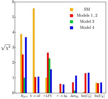
Figure 4.1: Contribution to $\sqrt{\chi^{2}}$ coming from each observable for models 1-4.

We distinguish three different non-SM fits, given that Models 1 and 2 are described by an equivalent set of effective parameters. The contribution to $(\chi^{2}_{\mathrm{min}})^{1/2}$ (or the pull of the fit) from the various observables in the three different cases, vs. the SM one, is reported in Figure 4.1. The best fit points for the model parameters are reported in Table 4.

A few details about the fit procedure are in order. Since $s_{e}$ is constrained only by $K_{L}\to\mu e$, in all cases we set $s_{e}=0$ and treat this parameter (as well as $K_{L}\to\mu e$) separately. In models 1,2,3 we assume $s_{l_{1}}=s_{q_{1}}=0$ and $s_{l_{3}}=s_{q_{3}}=1$. We further implement the requirement that $U(2)^{n}_{f}$ breaking should not exceed its natural size dictated by the structure of the SM Yukawa couplings, adding a smooth gaussian contribution with $\sigma=0.05$ to the $\chi^{2}$ for $\left|s_{\tau,b,q_{2},l_{2}}\right|>0.1$ and $\left|\theta_{d}\right|>0.3$. Additionally, we impose a smooth gaussian contribution for $\left|\theta_{\chi_{2}}\right|>0.5$. For Model 4, on top of adding a smooth gaussian contribution with $\sigma=0.05$ to the $\chi^{2}$ for $\left|s_{\tau}\right|>0.1$, we assume the following strict boundaries $\left|z_{u_{2},d_{2},e_{2},\nu_{2}}\right|<0.2$, $0.5<\left|z_{d_{3},u_{3},e_{3},\nu_{3}}\right|<1$, and $\left|z_{\nu_{1}}\right|<0.01$, again dictated by a natural flavour symmetry breaking structure.

case	$\chi^{2}_{\rm{min}}$	model parameters	best fit point	$1\sigma$
Model 1,2 $s_{d}$, $\alpha_{d}$ fixed $\theta_{\chi_{2}}$ free	$20.9(17.5)$	$m_{\rm eff}$ [TeV]	$0.76$	$[0.59,0.80]$
		$s_{q_{2}}$	$0.02$
		$s_{l_{2}}$	$0.18$
		$s_{\tau}$	$0.12$
		$s_{b}$	$0.004$
		$\theta_{\chi_{2}}$	$0.50$
		$\alpha_{\chi}$	$0.66$
Model 3    $s_{d}$, $\alpha_{d}$ free $\theta_{\chi_{2}}$ free	$6.8(6.2)$	$m_{\rm eff}$ [TeV]	$0.67$	$[0.66,0.92]$
		$s_{q_{2}}$	$0.13$
		$s_{l_{2}}$	$0.10$
		$s_{\tau}$	$0.10$
		$s_{b}$	$-0.002$
		$\theta_{\chi_{2}}$	$0.51$
		$\alpha_{\chi}$	$0$
		$\theta_{d}$	$-0.24$
		$\alpha_{d}$	$0.00005$
Model 4    minimal model	$23.7(20.9)$	$m_{\rm eff}$ [TeV]	$1.31$	$[0.93,1.35]$
		$z_{u_{2}}$	$0.02$
		$z_{u_{3}}$	$0.5$
		$z_{d_{2}}$	$-0.07$
		$z_{d_{3}}$	$-0.5$
		$z_{e_{2}}$	$0.2$
		$z_{e_{3}}$	$-1$
		$z_{\nu_{1}}$	$-0.01$
		$z_{\nu_{2}}$	$-0.2$
		$z_{\nu_{3}}$	$1$
		$s_{\tau}$	$0.17$

Table 4.2: Fit results for the different Models. In the $\chi^{2}_{\mathrm{min}}$ entry, the number in parenthesis is the contribution to $\chi^{2}_{\mathrm{min}}$ that comes solely from the observables. For reference, in the SM $\chi^{2}_{\rm{min,SM}}=47.6$.

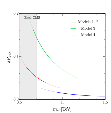
Figure 4.2: $\delta R_{D^{(\ast)}}$ as a function of $m_{\rm eff}$ varying $m_{\rm eff}$ in the $1\sigma$ (dark) and $2\sigma$ (light) region preferred by the fit. The remaining parameters entering $\delta R_{D^{(\ast)}}$ are fixed to the best-fit point. The grey band indicates the CMS exclusion at 700 GeV [35, 36, 37].

5 Discussion

From the analysis of the fit results, illustrated in Figures 4.1 and Table 4, we can deduce the following conclusions:

• In all models a strong lower bound on $m_{\rm eff}$ is set by LFU in $\tau$ decays. This limits the contribution to $\delta R_{D^{(\ast)}}$ from the pure third-generation semileptonic operator (in the down-quark mass basis) generated by the leptoquark exchange, i.e. the amplitude proportional to $C_{U}V_{cb}\beta^{U}_{b\tau}\beta^{U\ast}_{b\tau}$ in Eq. (A.3).

• In models 1, 2 and 3, if $\theta_{\chi_{2}}=O(1)$ and $s_{q_{2}}\not=0$, a sizeable effective coupling $\beta^{U}_{s\tau}\approx s_{\chi_{2}}s_{q_{2}}$ is generated. This can in turn yield an additional contribution to $\delta R_{D^{(\ast)}}$ proportional to $C_{U}V_{cs}\beta^{U}_{s\tau}\beta^{U\ast}_{b\tau}$. In Model 4, since there is no freedom in the flavour-changing interactions, we do not have such a possibility. Indeed, in this case it is not possible to generate a sizeable contribution to $R_{D^{(\ast)}}$. Additional constraints from $\Delta F=2$ observables drive the best-fit point for this model toward higher $m_{\rm eff}$ values.

• In models 1, 2 and 3, in order to reach the present central value of $\delta R_{D^{(\ast)}}$, we need not only $\theta_{\chi_{2}}=O(1)$ but also $s_{q_{2}}=O(0.1)$. The latter condition is phenomenologically viable only if we can adjust the parameters in $U_{d}$ (or $\hat{U}_{d}$) to minimize the $\Delta F=2$ amplitudes generated by the (tree-level) coloron exchange. While all models can satisfy the $B_{s}$ mixing bound in the $s_{b}\to 0$ limit, only in Model 3 is possible to adjust also $s_{d}$ and $\alpha_{d}$ in order to satisfy both $K-\bar{K}$ and $D-\bar{D}$ mixing bounds. As anticipated, this happens in the case of a real $2\times 2$ light block in $\hat{U}_{d}$.

• Also the constraint from $K_{L}\to\mu e$ is easily evaded. In particular, for the best fit point of Model 3, the $K_{L}\to\mu e$ bound implies the (weak) condition $|s_{e}|<0.6$.

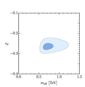
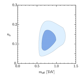
Figure 5.1: Two-dimensional preferred 1 and 2 $\sigma$ regions (in blue and light blue, respectively) for $m_{\rm eff}$ vs $s_{b}$, $s_{d}$, $s_{\tau}$, $s_{l_{2}}$ for Model 3.

A clear summary of the all these features is provided by the $\delta R_{D^{(\ast)}}$ vs. $m_{\rm eff}$ plot in Figure 4.2. As can be seen, only Model 3 is able to generate a contribution to $\delta R_{D^{(\ast)}}$ above $10\%$, provided $m_{\rm eff}$ lies close to its lower bound. In this figure, we also show the bound on $m_{\rm eff}$ obtained by searching for modifications of the Drell-Yan process $pp\to\tau^{+}\tau^{-}+X$ at high-energies, which is sensitive to the $t$-channel $U_{1}$ exchange [38, 39, 40]. A series of recent analyses by CMS of $pp\to\tau^{+}\tau^{-}+X$ [35, 36], and the related charged-current process $pp\to\tau\nu+X$ [37], allows us to set the bound $m_{\rm eff}\lower 3.01385pt\hbox{$\;\stackrel{{\scriptstyle\textstyle>}}{{\sim}}\;$}700$ GeV, with a tantalizing $3\sigma$ excess for $m_{\rm eff}\sim 800$ GeV [36].

Focusing on Model 3, in Figure 5.1 we illustrate the range of the mixing parameters determined by the fit. These plots provide a qualitative indication of the degree of flavour alignment necessary to successfully fit both sets of anomalies and, at the same time, satisfy all available constraints. As it can be seen, all parameters are compatible with their natural size, hence with the assumption of a mildly broken $U(2)^{n}_{f}$ symmetry. However, both $s_{d}$ and $s_{b}$ require a $10\%$ tuning with respect to their natural sizes: $s_{d}=O(\lambda)$ and $s_{b}=O(|V_{cb}|)$.

In summary, the proposal of a $U_{\mu}^{a}$ leptoquark, with couplings to fermions ruled by a mildly broken $U(2)^{n}_{f}$ flavour symmetry connected to the structure of the SM Yukawa couplings, originally formulated in [11], remains a very interesting option to address one or both sets of $B$ anomalies. The embedding of the $U_{\mu}^{a}$ in the adjoint of $SU(4)$, which is necessary for any realistic UV completion, makes this construction more constrained but still viable. In particular, addressing both sets of anomalies is possible only under rather specific conditions about the $U(2)^{n}_{f}$ symmetry breaking. The evolution of the experimental data in the near future will tell if (some of) the anomalies will persist and, in the positive case, in which direction their explanation in terms of $SU(4)$ vector leptoquarks will have to evolve. On general grounds, the relatively low value of $m_{\rm eff}$ that we found in all the simplified models we have considered makes the search for high-energy signatures of the leptoquark (and possibly the vector-like fermions) quite interesting in view of the high-luminosity phase of the LHC.

Acknowledgements

This project has received funding from the European Research Council (ERC) under the European Union’s Horizon 2020 research and innovation program under grant agreement 833280 (FLAY), and by the Swiss National Science Foundation (SNF) under contract 200020_204428. The research of C.C. was supported by the Cluster of Excellence Precision Physics, Fundamental Interactions, and Structure of Matter (PRISMA⁺ - EXC 2118/1) within the German Excellence Strategy (project ID 39083149). C.C. is grateful for the hospitality of Perimeter Institute where part of this work was carried out. Research at Perimeter Institute is supported in part by the Government of Canada through the Department of Innovation, Science and Economic Development Canada and by the province of Ontario through the Ministry of Economic Development, Job Creation and Trade. This research was also supported in part by the Simons Foundation through the Simons Foundation Emmy Noether Fellows Program at Perimeter Institute.

Appendix A Simplified expressions for low-energy observables

We denote the relative variation of an observable $O$ with respect to the SM by $\delta(O)$, with

$$\delta(O)=\frac{O-O_{\mathrm{SM}}}{O_{\mathrm{SM}}}\,.$$ (A.1)

$b\to sll$ and $b\to cl\nu$

$$C_{9,\mathrm{NP}}^{\mu}=-C_{10,\mathrm{NP}}^{\mu}=-\frac{2\pi}{\alpha V_{ts}^{\ast}V_{tb}}\left(C_{U}\beta^{U}_{s\mu}\beta^{U\ast}_{b\mu}-\frac{C_{X}}{4}\beta^{X}_{sb}\beta^{X}_{\mu\mu}\right)$$ (A.2)

$$\delta R_{D^{(\ast)}}^{\tau/\mu}=2C_{U}\mathrm{Re}\left[\frac{\beta^{U\ast}_{b\tau}\beta^{U}_{c\nu_{\tau}}-\beta^{U\ast}_{b\mu}\beta^{U}_{c\nu_{\mu}}}{V_{cb}}\right]\approx 2C_{U}\mathrm{Re}\left[\frac{V_{cb}\beta^{U\ast}_{b\tau}\beta^{U}_{b\tau}+V_{cs}\beta^{U\ast}_{b\tau}\beta^{U}_{s\tau}}{V_{cb}}\right]$$ (A.3)

Universality tests in leptonic $\tau$ decays

$$\left(\frac{g_{\alpha}}{g_{\beta}}\right)_{\ell}=\left[\frac{\mathcal{B}(\ell_{\alpha}\to\ell_{\rho}\,\nu\bar{\nu})_{\rm exp}/\mathcal{B}(\ell_{\alpha}\to\ell_{\rho}\,\nu\bar{\nu})_{\rm SM}}{\mathcal{B}(\ell_{\beta}\to\ell_{\rho}\,\nu\bar{\nu})_{\rm exp}/\mathcal{B}(\ell_{\beta}\to\ell_{\rho}\,\nu\bar{\nu})_{\rm SM}}\right]^{\frac{1}{2}}\,.$$ (A.4)

$$\left(\frac{g_{\tau}}{g_{\mu}}\right)_{\ell} =1+\frac{9}{12}C_{X}\left(\left|\beta^{X}_{\tau e}\right|^{2}-\left|\beta^{X}_{\mu e}\right|^{2}\right)-\eta\,C_{U}\left(\left|\beta^{U}_{b\tau}\right|^{2}-\left|\beta^{U}_{b\mu}\right|^{2}\right)$$ (A.5)

$$\left(\frac{g_{\tau}}{g_{e}}\right)_{\ell} =1+\frac{9}{12}C_{X}\left(\left|\beta^{X}_{\tau\mu}\right|^{2}-\left|\beta^{X}_{\mu e}\right|^{2}\right)-\eta\,C_{U}\left(\left|\beta^{U}_{b\tau}\right|^{2}-\left|\beta^{U}_{be}\right|^{2}\right)$$ (A.6)

Neglecting the $X$ contribution and using the fact that $\left|\beta^{U}_{b\mu,e}\right|\ll\left|\beta^{U}_{b\tau}\right|$, we have:

$$\left(\frac{g_{\tau}}{g_{\mu}}\right)_{\ell}\approx\left(\frac{g_{\tau}}{g_{e}}\right)_{\ell}\approx 1-\eta\,C_{U}\left|\beta^{U}_{b\tau}\right|^{2}\,,$$ (A.7)

where the running $\eta=0.079$ is computed assuming $\Lambda=2\,\mathrm{TeV}$.

$\tau-\mu$ LFV

$$\mathcal{B}(\tau\to 3\mu)=\frac{9}{8}C_{X}^{2}\left|\beta_{\mu\tau}^{X}\beta_{\mu\mu}^{X}\right|^{2}\mathcal{B}(\tau\to\mu\bar{\nu}\nu)_{\mathrm{SM}}$$ (A.8)

$\Delta F=2$ observables

Effective Lagrangian for the $\Delta F=2$ mixing amplitudes:

$$\begin{aligned} \mathcal{L}^{\Delta F=2}=-C_{bs}\left(\bar{b}_{L}\gamma_{\mu}s_{L}\right)^{2}-C_{bd}\left(\bar{b}_{L}\gamma_{\mu}d_{L}\right)^{2}-C_{uc}\left(\bar{u}_{L}\gamma_{\mu}c_{L}\right)^{2}+\text{h.c.}\,,\end{aligned}$$ (A.9)

NP contribution to these Wilson coefficients:

$$\begin{aligned} C_{bs}^{\mathrm{NP}}&=\frac{2}{v^{2}}\left(\frac{C_{G}}{3}\left.\beta^{G}_{bs}\right.^{2}+\frac{C_{X}}{24}\left.\beta^{X}_{bs}\right.^{2}\right)\\ C_{ds}^{\mathrm{NP}}&=\frac{2}{v^{2}}\left(\frac{C_{G}}{3}\left.\beta^{G}_{ds}\right.^{2}+\frac{C_{X}}{24}\left.\beta^{X}_{ds}\right.^{2}\right)\\ C_{uc}^{\mathrm{NP}}&=\frac{2}{v^{2}}\left(\frac{C_{G}}{3}\left.\beta^{G,u}_{uc}\right.^{2}+\frac{C_{X}}{24}\left.\beta^{X,u}_{uc}\right.^{2}\right)\end{aligned}$$ (A.10)

Main observables are $\mathrm{Im}[C_{uc}^{\mathrm{NP}}]$, $\mathrm{Im}[C_{ds}^{\mathrm{NP}}]$ and $\delta(\Delta m_{B_{s}})$. The latter is defined as

$$\delta(\Delta m_{B_{s}})=\left|1+\frac{C^{\rm NP}_{bs}}{C_{bs}^{\rm SM}}\right|-1\,,$$ (A.11)

where

$$C^{\rm SM}_{bs}=\frac{G_{F}^{2}m_{W}^{2}}{4\pi^{2}}\,\big{(}V_{tb}^{*}V_{ts}\big{)}^{2}\,S_{0}(x_{t})\,,$$ (A.12)

with $x_{t}=\frac{m_{t}^{2}}{m_{W}^{2}}$ and $S_{0}(x_{t})\approx 2.37$.

$\mu-e$ LFV

$$\begin{aligned} \mathcal{B}(K_{L}^{0}\to\mu^{-}e^{+})&=\frac{\tau_{K_{L}}G_{F}^{2}f_{K}^{2}m_{\mu}^{2}m_{K}}{8\pi}\left(1-\frac{m_{\mu}^{2}}{m_{K}^{2}}\right)^{2}\left|C_{U}\left(\beta^{U}_{de}\beta^{U\ast}_{s\mu}+\beta^{U}_{se}\beta^{U\ast}_{d\mu}\right)-\frac{C_{X}}{4}2\mathrm{Re}\left[\beta^{X}_{ds}\right]\beta^{X}_{\mu e}\right|^{2}\\ \mathcal{B}(K_{L}^{0}\to\mu^{+}e^{-})&=\frac{\tau_{K_{L}}G_{F}^{2}f_{K}^{2}m_{\mu}^{2}m_{K}}{8\pi}\left(1-\frac{m_{\mu}^{2}}{m_{K}^{2}}\right)^{2}\left|C_{U}\left(\beta^{U}_{d\mu}\beta^{U\ast}_{se}+\beta^{U}_{s\mu}\beta^{U\ast}_{de}\right)-\frac{C_{X}}{4}2\mathrm{Re}\left[\beta^{X}_{ds}\right]\beta^{X}_{e\mu}\right|^{2}\end{aligned}$$ (A.13)

$$\mathcal{B}(\mu\to 3e) =\frac{9}{8}C_{X}^{2}\left|\beta_{e\mu}^{X}\beta_{ee}^{X}\right|^{2}\mathcal{B}(\mu\to e\bar{\nu}\nu)_{\mathrm{SM}}$$ (A.14)

References

- [1] LHCb collaboration, R. Aaij et al., Test of lepton universality using decays, Phys. Rev. Lett. 113 (2014) 151601, [1406.6482].
- [2] LHCb collaboration, R. Aaij et al., Test of lepton universality with decays, JHEP 08 (2017) 055, [1705.05802].
- [3] LHCb collaboration, R. Aaij et al., Search for lepton-universality violation in decays, Phys. Rev. Lett. 122 (2019) 191801, [1903.09252].
- [4] LHCb collaboration, R. Aaij et al., Test of lepton universality in beauty-quark decays, Nature Phys. 18 (2022) 277–282, [2103.11769].
- [5] BaBar collaboration, J. P. Lees et al., Evidence for an excess of decays, Phys. Rev. Lett. 109 (2012) 101802, [1205.5442].
- [6] BaBar collaboration, J. P. Lees et al., Measurement of an Excess of Decays and Implications for Charged Higgs Bosons, Phys. Rev. D 88 (2013) 072012, [1303.0571].
- [7] Belle collaboration, M. Huschle et al., Measurement of the branching ratio of relative to decays with hadronic tagging at Belle, Phys. Rev. D 92 (2015) 072014, [1507.03233].
- [8] LHCb collaboration, R. Aaij et al., Measurement of the ratio of branching fractions , Phys. Rev. Lett. 115 (2015) 111803, [1506.08614].
- [9] LHCb collaboration, R. Aaij et al., Measurement of the ratio of the and branching fractions using three-prong -lepton decays, Phys. Rev. Lett. 120 (2018) 171802, [1708.08856].
- [10] LHCb collaboration, R. Aaij et al., Test of Lepton Flavor Universality by the measurement of the branching fraction using three-prong decays, Phys. Rev. D 97 (2018) 072013, [1711.02505].
- [11] R. Barbieri, G. Isidori, A. Pattori and F. Senia, Anomalies in -decays and flavour symmetry, Eur. Phys. J. C 76 (2016) 67, [1512.01560].
- [12] R. Alonso, B. Grinstein and J. Martin Camalich, Lepton universality violation and lepton flavor conservation in -meson decays, JHEP 10 (2015) 184, [1505.05164].
- [13] L. Calibbi, A. Crivellin and T. Ota, Effective Field Theory Approach to , and with Third Generation Couplings, Phys. Rev. Lett. 115 (2015) 181801, [1506.02661].
- [14] D. Buttazzo, A. Greljo, G. Isidori and D. Marzocca, B-physics anomalies: a guide to combined explanations, JHEP 11 (2017) 044, [1706.07808].
- [15] R. Barbieri, C. W. Murphy and F. Senia, B-decay Anomalies in a Composite Leptoquark Model, Eur. Phys. J. C 77 (2017) 8, [1611.04930].
- [16] L. Di Luzio, A. Greljo and M. Nardecchia, Gauge leptoquark as the origin of B-physics anomalies, Phys. Rev. D 96 (2017) 115011, [1708.08450].
- [17] R. Barbieri and A. Tesi, -decay anomalies in Pati-Salam SU(4), Eur. Phys. J. C 78 (2018) 193, [1712.06844].
- [18] M. Bordone, C. Cornella, J. Fuentes-Martin and G. Isidori, A three-site gauge model for flavor hierarchies and flavor anomalies, Phys. Lett. B 779 (2018) 317–323, [1712.01368].
- [19] A. Greljo and B. A. Stefanek, Third family quark–lepton unification at the TeV scale, Phys. Lett. B 782 (2018) 131–138, [1802.04274].
- [20] C. Cornella, J. Fuentes-Martin and G. Isidori, Revisiting the vector leptoquark explanation of the B-physics anomalies, JHEP 07 (2019) 168, [1903.11517].
- [21] J. Fuentes-Martín and P. Stangl, Third-family quark-lepton unification with a fundamental composite Higgs, Phys. Lett. B 811 (2020) 135953, [2004.11376].
- [22] J. Fuentes-Martin, G. Isidori, J. M. Lizana, N. Selimovic and B. A. Stefanek, Flavor hierarchies, flavor anomalies, and Higgs mass from a warped extra dimension, 2203.01952.
- [23] J. Fuentes-Martin, G. Isidori, J. Pagès and B. A. Stefanek, Flavor non-universal Pati-Salam unification and neutrino masses, Phys. Lett. B 820 (2021) 136484, [2012.10492].
- [24] R. Barbieri, G. Isidori, J. Jones-Perez, P. Lodone and D. M. Straub, and Minimal Flavour Violation in Supersymmetry, Eur. Phys. J. C 71 (2011) 1725, [1105.2296].
- [25] R. Barbieri, D. Buttazzo, F. Sala and D. M. Straub, Flavour physics from an approximate symmetry, JHEP 07 (2012) 181, [1203.4218].
- [26] G. Blankenburg, G. Isidori and J. Jones-Perez, Neutrino Masses and LFV from Minimal Breaking of and flavor Symmetries, Eur. Phys. J. C 72 (2012) 2126, [1204.0688].
- [27] J. Fuentes-Martín, G. Isidori, J. Pagès and K. Yamamoto, With or without U(2)? Probing non-standard flavor and helicity structures in semileptonic B decays, Phys. Lett. B 800 (2020) 135080, [1909.02519].
- [28] O. L. Crosas, G. Isidori, J. M. Lizana, N. Selimovic and B. A. Stefanek, Flavor Non-universal Vector Leptoquark Imprints in and Transitions, 2207.00018.
- [29] W. Altmannshofer and P. Stangl, New physics in rare B decays after Moriond 2021, Eur. Phys. J. C 81 (2021) 952, [2103.13370].
- [30] HFLAV collaboration, Y. Amhis et al., Averages of -hadron, -hadron, and -lepton properties as of 2021, 2206.07501.
- [31] F. Feruglio, P. Paradisi and A. Pattori, Revisiting Lepton Flavor Universality in B Decays, Phys. Rev. Lett. 118 (2017) 011801, [1606.00524].
- [32] “Flavor constraints on new physics.” https://agenda.infn.it/event/14377/contributions/24434/attachments/17481/19830/silvestriniLaThuile.pdf.
- [33] UTfit collaboration, M. Bona et al., Model-independent constraints on operators and the scale of new physics, JHEP 03 (2008) 049, [0707.0636].
- [34] Particle Data Group collaboration, P. A. Zyla et al., Review of Particle Physics, PTEP 2020 (2020) 083C01.
- [35] CMS collaboration, “CMS-PAS-HIG-21-001.” https://cds.cern.ch/record/2803739/files/HIG-21-001-pas.pdf.
- [36] CMS collaboration, “CMS-PAS-EXO-19-016.” http://cds.cern.ch/record/2815309/files/EXO-19-016-pas.pdf.
- [37] CMS collaboration, “CMS-PAS-EXO-21-009.” http://cds.cern.ch/record/2815310/files/EXO-21-009-pas.pdf.
- [38] D. A. Faroughy, A. Greljo and J. F. Kamenik, Confronting lepton flavor universality violation in B decays with high- tau lepton searches at LHC, Phys. Lett. B 764 (2017) 126–134, [1609.07138].
- [39] M. Schmaltz and Y.-M. Zhong, The leptoquark Hunter’s guide: large coupling, JHEP 01 (2019) 132, [1810.10017].
- [40] M. J. Baker, J. Fuentes-Martin, G. Isidori and M. König, High– signatures in vector-leptoquark models, Eur. Phys. J. C 79 (2019) 334, [1901.10480].