Leptogenesis and Dark Matter Through Relativistic Bubble Walls with Observable Gravitational Waves

Abstract

We study a scenario where both dark matter and heavy right handed neutrino (RHN) responsible for leptogenesis acquire masses by crossing the relativistic bubble walls formed as a result of a TeV scale supercooled first order phase transition (FOPT). While this leads to a large out-of-equilibrium abundance of right handed neutrino inside the bubble sufficient to produce the required lepton asymmetry, the dark matter being lighter can still remain in equilibrium with its relic being set by subsequent thermal freeze-out. A classical conformal symmetry ensures the origin of mass via FOPT induced by a singlet scalar while also ensuring supercooling leading to enhanced gravitational wave amplitude within the sensitivity of the LISA experiment. A minimal scenario with three RHN, one inert scalar doublet and one singlet scalar as additional fields beyond the standard model is sufficient to realize this possibility which also favours inert RHN dark matter over inert scalar doublet.

I Introduction

The observed baryon asymmetry of the universe (BAU) has been a longstanding puzzle in cosmology and particle physics. While only around $5\%$ of the present universe is made up of baryonic matter, the observed excess of baryons over anti-baryons is quoted in terms of the baryon to photon ratio as Aghanim:2018eyx

$$\eta_{B}=\frac{n_{B}-n_{\overline{B}}}{n_{\gamma}}\simeq 6.2\times 10^{-10},$$ (1)

based on the cosmic microwave background (CMB) measurements which also agrees well with the big bang nucleosynthesis (BBN) estimates Zyla:2020zbs . Assuming the universe to start in a matter-antimatter symmetric manner, the observed BAU can be generated dynamically if certain conditions, known as the Sakharov’s conditions Sakharov:1967dj are satisfied. Since the standard model (SM) fails to satisfy these criteria in required amount, several ways of generating the BAU has been proposed. In one such popular scenario, known as baryogenesis Weinberg:1979bt ; Kolb:1979qa , out-of-equilibrium decay of a heavy particle is responsible for generating the observed BAU. One interesting way to achieve baryogenesis is leptogenesis Fukugita:1986hr where a non-zero lepton asymmetry is first generated which later gets converted into the BAU via electroweak sphalerons Kuzmin:1985mm . While this asymmetric baryonic matter comprises $5\%$ of the present universe, the total matter content of the universe is around $32\%$ with the significant portion being in the form of a non-luminous, non-baryonic form of matter, known as dark matter (DM). While relative abundance of DM is approximately $27\%$, it is conventionally reported in terms of density parameter $\Omega_{\rm DM}$ and reduced Hubble constant $h=\text{Hubble Parameter}/(100\;\text{km}~{}\text{s}^{-1}\text{Mpc}^{-1})$ as Aghanim:2018eyx

$$\Omega_{\text{DM}}h^{2}=0.120\pm 0.001$$ (2)

at 68% CL. Similar to BAU, there is no explanation for DM in the SM, leading to a plethora of beyond standard model (BSM) scenarios. The weakly interacting massive particle (WIMP) paradigm has been the most widely studied particle DM scenario where a DM particle having mass and interactions around the electroweak ballpark naturally gives rise to the observed DM relic via thermal freeze-out, a remarkable coincidence often referred to as the WIMP Miracle.

In generic seesaw scenarios, there exists a lower bound on the scale of leptogenesis $M_{1}>10^{9}$ GeV, known as the Davidson-Ibarra bound Davidson:2002qv if such asymmetries arise from out-of-equilibrium decay. This keeps the scale of leptogenesis far away from any direct experimental probe. In scenarios where lepton asymmetry is generated from decay, introduction of additional fields on top of the ones required to implement a generic seesaw model of neutrino mass, can alleviate such strong lower bound on the scale of leptogenesis LeDall:2014too ; Alanne:2018brf ; Hambye:2009pw ; Racker:2013lua ; Clarke:2015hta ; Hugle:2018qbw ; Borah:2018rca ; Mahanta:2019gfe ; Mahanta:2019sfo ; Sarma:2020msa ; Borah:2020ivi . Even in such leptogenesis from decay type scenarios, there is another way to have TeV scale leptogenesis by resonant enhancement of the CP asymmetry, known as the resonant leptogenesis Pilaftsis:1998pd ; Pilaftsis:2003gt with fine-tuned mass splitting between decaying particles. Even for such TeV scale leptogenesis, the decaying particle say, a right handed neutrino, has very tiny couplings with leptons in order to satisfy light neutrino masses, making it difficult to probe it directly. Thus, leptogenesis from decay, in general, has limited direct experimental probe Chun:2017spz . This has led to some recent attempts in finding ways to probe leptogenesis via stochastic gravitational wave (GW) observation Dror:2019syi ; Blasi:2020wpy ; Fornal:2020esl ; Samanta:2020cdk ; Barman:2022yos ; Baldes:2021vyz ; Azatov:2021irb ; Huang:2022vkf ; Dasgupta:2022isg . While some of these works rely upon topological defects like cosmic strings, domain walls formed as a result of symmetry breaking Dror:2019syi ; Blasi:2020wpy ; Fornal:2020esl ; Samanta:2020cdk ; Barman:2022yos , others consider a first order phase transition (FOPT) to be responsible for generating GW Baldes:2021vyz ; Azatov:2021irb ; Huang:2022vkf ; Dasgupta:2022isg . Similarly, there have been attempts in finding complementary DM probes like stochastic GW background Yuan:2021ebu ; Tsukada:2020lgt ; Chatrchyan:2020pzh ; Bian:2021vmi ; Samanta:2021mdm ; Borah:2022byb ; Azatov:2021ifm ; Azatov:2022tii ; Baldes:2022oev , specially in view of the continued null results at direct detection experiments LUX-ZEPLIN:2022qhg .

Motivated by this, we consider a minimal scenario where both leptogenesis and DM are triggered by a strong first order phase transition with observable GW signatures. Similar to the baryogenesis mechanism adopted in Baldes:2021vyz followed by leptogenesis implementation in Huang:2022vkf ; Dasgupta:2022isg , we consider a scenario where DM as well as right handed neutrino responsible for leptogenesis acquire masses in a FOPT by crossing the relativistic bubble walls. Unlike additional gauge symmetries considered in these works, here we consider a minimal scenario without any gauge extension of the SM. Adopting a classical conformal symmetry required to generate masses of gauge singlet fermions via FOPT as well as to enhance the strength via supercooling, we first consider the conformal version of the minimal scotogenic model Ma:2006km . While this model contains DM as well as right handed neutrino (RHN) responsible for leptogenesis, we find that it is not possible to get the desired leptogenesis from RHN decay. This is due to strict constraints on the hierarchy of massive fields like DM and RHNs coupling to the singlet scalar field which is also driving the FOPT. We then adopt a hybrid setup with type I and scotogenic origin of light neutrino masses and discuss the resulting phenomenology of DM, leptogenesis and GW. With only five additional BSM fields, the model remains successful and predictive at experiments operational at different frontiers.

This paper is organised as follows. In section II we briefly discuss the conformal version of the scotogenic model followed by the details of first order phase transition in section III. In section IV, we discuss the details of gravitational wave production followed by discussion of leptogenesis and dark matter in section V. Finally, we conclude in section VI.

II Conformal Scotogenic Model

In order to realize a supercooled phase transition along with leptogenesis and dark matter, we first consider the conformal or scale invariant version Ahriche:2016cio of the minimal scotogenic model Ma:2006km where the SM is extended by three gauge singlet right handed neutrinos $N_{i}$ (with $i=1,2,3$), one additional scalar doublet $\eta$. An additional $Z_{2}$ symmetry is imposed under which these newly added particles are odd while all SM particles are even. In order to preserve the conformal nature and generate masses, an additional $Z_{2}$ even singlet scalar S is introduced.

The leptonic Yukawa Lagrangian relevant for light neutrino mass is

$${\cal L}\ \supset\ \frac{1}{2}Y^{\prime}_{ij}SN_{i}N_{j}+\left(Y_{ij}\,\bar{L}_{i}\tilde{\eta}N_{j}+\text{h.c.}\right)\ .$$ (3)

Clearly, there is no coupling of neutrinos to the SM Higgs doublet $\Phi_{1}$ due to the unbroken $Z_{2}$ symmetry. However, light neutrino masses arise at radiative level with $Z_{2}$ odd particles taking part in the loop.

The scalar potential of the model can be written as

$$V(\Phi_{1},\eta,S) \ =\ \frac{\lambda_{1}}{4}|\Phi_{1}|^{4}+\frac{\lambda_{2}}{4}|\eta|^{4}+\lambda_{3}|\Phi_{1}|^{2}|\eta|^{2}+\frac{1}{4}\lambda_{S}S^{4}+\lambda_{4}|\Phi_{1}^{\dagger}\eta|^{2}+\left[\frac{\lambda_{5}}{2}(\Phi_{1}^{\dagger}\eta)^{2}+\text{h.c.}\right]$$

$$\qquad+\lambda_{6}|\Phi_{1}|^{2}S^{2}+\lambda_{7}|\eta|^{2}S^{2}\,.$$ (4)

where $\Phi_{1}$ is the SM Higgs doublet. Light neutrino masses which arise at one loop level can be evaluated as  Ma:2006km ; Merle:2015ica

$$(m_{\nu})_{ij}\ =\ \sum_{k}\frac{Y_{ik}Y_{jk}M_{k}}{32\pi^{2}}\left(\frac{m^{2}_{H^{0}}}{m^{2}_{H^{0}}-M^{2}_{k}}\>\text{ln}\frac{m^{2}_{H^{0}}}{M^{2}_{k}}-\frac{m^{2}_{A^{0}}}{m^{2}_{A^{0}}-M^{2}_{k}}\>\text{ln}\frac{m^{2}_{A^{0}}}{M^{2}_{k}}\right)$$

$$\ \equiv\ \sum_{k}\frac{Y_{ik}Y_{jk}M_{k}}{32\pi^{2}}\left[L_{k}(m^{2}_{H^{0}})-L_{k}(m^{2}_{A^{0}})\right]\,,$$ (5)

where $M_{k}$ is the mass eigenvalue of the mass eigenstate $N_{k}$ in the internal line and the indices $i,j=1,2,3$ run over the three neutrino generations as well as three copies of $N_{i}$. Also, $A^{0},H^{0}$ are the neutral pseudoscalar and scalar respectively contained in $\eta$. The function $L_{k}(m^{2})$ is defined as

$$L_{k}(m^{2})\ =\ \frac{m^{2}}{m^{2}-M^{2}_{k}}\>\text{ln}\frac{m^{2}}{M^{2}_{k}}\,.$$ (6)

Using the physical scalar mass expressions Mahanta:2019sfo , one can write $m^{2}_{H^{0}}-m^{2}_{A^{0}}=\lambda_{5}v^{2}_{\rm ew}$ where $v_{\rm ew}$ is the vacuum expectation value (VEV) of SM Higgs doublet. Thus, light neutrino mass is directly proportional to the parameter $\lambda_{5}$. In upcoming discussions, we will discuss the effects of $\lambda_{5}$ in details.

III First order phase transition

Here we are interested in the phase transition driven by the singlet scalar field at a scale above the electroweak scale as preferred from leptogenesis point of view. For electroweak phase transition in minimal scotogenic model without any conformal symmetry or singlet scalar, please refer to earlier work Borah:2020wut .

In order to study the details of FOPT in conformal scotogenic model, we first write down the full one-loop potential which can be schematically divided into following form:

$$V_{\rm tot}=V_{\rm tree}+V_{\rm CW}+V_{\rm th},$$ (7)

where $V_{\rm tree},~{}V_{\rm CW}$ and $V_{\rm th}$ denote the tree level scalar potential, the one-loop Coleman-Weinberg potential, the thermal effective potential, respectively. The tree level scalar potential is given by Eq. (4). In finite-temperature field theory, the effective potential, $V_{\rm CW}$ and $V_{\rm thermal}$, are calculated by using standard background field method Dolan:1973qd ; Quiros:1999jp . In the following calculations, we take Landau gauge for simplicity.

The Coleman-Weinberg potential Coleman:1973jx with $\overline{\rm DR}$ regularisation is given by

$$V_{\rm CW}=\sum_{i}(-)^{n_{f}}\frac{n_{i}}{64\pi^{2}}m_{i}^{4}(\phi)\left(\log\left(\frac{m_{i}^{2}(\phi)}{\mu^{2}}\right)-\frac{3}{2}\right),$$ (8)

where suffix $i$ represents particle species, and $n_{i},~{}m_{i}(\phi)$ are the degrees of freedom (dof) and field dependent masses of $i$’th particle. In addition, $\mu$ is the renormalisation scale, and $(-)^{n_{f}}$ is $+1$ for bosons and $-1$ for fermions, respectively. Since we are tracking the singlet scalar field for FOPT, we consider its VEV, denoted by $M$ as the renormalisation scale as $\mu=M=\langle S\rangle$. We denote the singlet scalar as $S=(\phi+M)/\sqrt{2}$. The relevant field dependent masses along with their dof are

$$m_{\eta}^{2}=\lambda_{7}\phi^{2}/2\;(n_{\eta}=4),m_{s}^{2}=3\lambda_{s}\phi^{2}\;(n_{s}=1),m_{y_{i}}^{2}=2y_{i}^{2}\phi^{2}\;(n_{y}=2)$$ (9)

Thermal contributions to the effective potential are given by

$$V_{\rm th}=\sum_{i}\left(\frac{n_{\rm B_{i}}}{2\pi^{2}}T^{4}J_{B}\left[\frac{m_{\rm B_{i}}}{T}\right]-\frac{n_{\rm F_{i}}}{2\pi^{2}}T^{4}J_{F}\left[\frac{m_{\rm F_{i}}}{T}\right]\right),$$ (10)

where $n_{B_{i}}$ and $n_{F_{i}}$ denote the dof of the bosonic and fermionic particles, respectively. In this expressions, $J_{B}$ and $J_{F}$ functions are defined by following functions:

$$J_{B}(x)=\int^{\infty}_{0}dzz^{2}\log\left[1-e^{-\sqrt{z^{2}+x^{2}}}\right],$$ (11)

$$J_{F}(x)=\int^{\infty}_{0}dzz^{2}\log\left[1+e^{-\sqrt{z^{2}+x^{2}}}\right].$$ (12)

In the calculation of the thermal potential, we also consider the contribution from the daisy diagrams such that the total thermal potential reads $V_{T}(\phi,T)=V_{\rm th}+V_{\rm daisy}(\phi,T)$. This has to be done in order to improve the perturbative expansion during the FOPT Fendley:1987ef ; Parwani:1991gq ; Arnold:1992rz . Such corrections can be implemented in two ways by inserting thermal masses into the zero-temperature field dependent masses. In one of these resummation prescriptions, known as the Parwani method Parwani:1991gq , thermal corrected field dependent masses are used. In the other prescription, known as the Arnold-Espinosa method Arnold:1992rz , the effect of the daisy diagram is included only for Matsubara zero-modes inside $J_{B}$ function defined above. In our work, we use the Arnold-Espinosa method. The thermal part of the potential, including the daisy contributions can now be written as

$$V_{T}(\phi,T) =V_{\rm th}+V_{\rm daisy}(\phi,T),$$ (13)

$$V_{\rm daisy}(\phi,T) =-\sum_{i}\frac{g_{i}T}{12\pi}\left[m^{3}_{i}(\phi,T)-m^{3}_{i}(\phi)\right],$$

wherein, $V_{\rm th}$ is the thermal correction and $V_{\rm daisy}$ is the daisy subtraction Fendley:1987ef ; Parwani:1991gq ; Arnold:1992rz . Denoting $m^{2}_{i}(\phi,T)=m^{2}_{i}(\phi)+\Pi_{i}(T)$, the relevant thermal masses can be written as Cline:2008hr

$$\Pi_{\eta}(T)=(\frac{g_{2}^{2}}{8}+\frac{g_{1}^{2}+g_{2}^{2}}{16}+\frac{\lambda_{2}}{2}+\frac{\lambda_{3}+\lambda_{4}}{12})T^{2}$$

$$\Pi_{s}(T)=(\frac{\lambda_{s}}{4}+\frac{\lambda_{6}}{3}+\frac{\lambda_{7}}{3}+\frac{y_{1}^{2}}{8}+\frac{y_{2}^{2}}{8}+\frac{y_{2}^{2}}{8})T^{2}.$$

The FOPT proceeds via tunnelling, and the corresponding spherical symmetric field configurations known as bubbles are nucleated followed by expansion and coalescence. For recent reviews of FOPT in cosmological context, please refer to Mazumdar:2018dfl ; Hindmarsh:2020hop . The tunnelling rate per unit time per unit volume can be estimated as

$$\Gamma(T)=\mathcal{A}(T)e^{-S_{3}(T)/T},$$ (14)

where $\mathcal{A}(T)\sim T^{4}$ and $S_{3}(T)$ are determined by the dimensional analysis and given by the classical configurations, called bounce, respectively. At finite temperature, the $O(3)$ symmetric bounce solution Linde:1980tt can be obtained by solving the following equation

$$\frac{d^{2}\phi}{dr^{2}}+\frac{2}{r}\frac{d\phi}{dr}=\frac{\partial V_{\rm tot}}{\partial\phi}.$$ (15)

The boundary conditions required to solve the above differential equation are

$$\phi(r\to\infty)=\phi_{\rm false},~{}~{}~{}\left.\frac{d\phi}{dr}\right|_{r=0}=0,$$ (16)

where $\phi_{\rm false}$ denotes the position of the false vacuum. Using $\phi$ governed by the above equation and boundary conditions, the bounce action can be written as

$$S_{3}=\int_{0}^{\infty}dr4\pi r^{2}\left[\frac{1}{2}\left(\frac{d\phi}{dr}\right)^{2}+V_{\rm tot}(\phi,T)\right].$$ (17)

The temperature at which the bubbles are nucleated is called the nucleation temperature $T_{n}$. This can be calculated by comparing the tunnelling rate to the Hubble expansion rate as

$$\Gamma(T_{n})={\bf H}^{4}(T_{n}).$$ (18)

Here, assuming the usual radiation dominated universe, the Hubble parameter is given by ${\bf H}(T)\simeq 1.66\sqrt{g_{*}}T^{2}/M_{\rm Pl}$ with $g_{*}$ being the dof of the radiation component. Thus, the rate comparison equation above leads to

$$\frac{S_{3}(T_{n})}{T_{n}}\simeq 140,$$ (19)

for $g_{*}\sim 100$ and $T_{n}\sim 100$ GeV while for lower temperature near MeV where $g_{*}\sim 10$, the above ratio becomes larger. For higher nucleation temperature, as we have in the present scenario, the ratio $\frac{S_{3}(T_{n})}{T_{n}}$ becomes smaller than the one quoted above. If $\phi(T_{n})/T_{n}>1$ is satisfied, where $\phi(T_{n})$ is the singlet scalar VEV at the nucleation temperature, $T=T_{n}$, the corresponding phase transition is conventionally called strong first order. Alternatively, the ratio at critical temperature namely $\phi(T_{c})/T_{c}\equiv v_{c}/T_{c}>1$ is also used as the strength of the FOPT. The critical temperature $T_{c}$ corresponds to the temperature where the two minima of the potential are degenerate.

	$v_{c}$ (GeV)	$T_{c}$ (GeV)	v (GeV)	$v_{c}/T_{c}$	$\lambda_{7}(0)$	$Y^{\prime}(0)$	$\lambda_{s}(0)$
BP1	9540.78	2374	9901.77	4.01	1.5	0.5	0.02
BP2	9599.59	2407	9968.24	3.98	1.6	0.4	0.02
BP3	9734.10	2422	9997.27	4.01	1.2	0.2	0.02
BP4	9648.57	2391	9988.00	4.03	1.4	0.3	0.02

Table 1: Benchmark parameters of the model and other details of the FOPT in conformal scotogenic model.

In order to simplify the bounce calculation, we write the zero temperature one-loop effective potential as Jinno:2016knw ; Iso:2009nw

$$V_{0} =V_{\rm tree}+V_{\rm CW},$$

$$=\frac{1}{4}\lambda_{S}(t)G^{4}(t)\phi^{4}$$ (20)

where $t={\rm log}(\phi/\mu)$ with $\mu=M$ being the scale of renormalisation. $G(t)$ is given by

$$G(t)=e^{-\int^{t}_{0}dt^{\prime}\gamma(t^{\prime})},\;\gamma(t)=\frac{1}{32\pi^{2}}{\rm Tr}[Y^{\prime\dagger}Y^{\prime}],$$ (21)

The Yukawa couplings and quartic coupling at the renormalisation scale are calculated by solving the renormalisation group evolution (RGE) equations of the model given in Appendix A. Taking the renormalisation scale $\mu$ to be $M$, the condition $\frac{dV}{d\phi}|_{\phi=M}=0$ leads us to the relation,

$$10\lambda^{2}_{s}(0)+32\pi^{2}\lambda_{s}(0)+3Y^{\prime 2}(0)\lambda_{s}(0)-3Y^{\prime 4}(0)+\lambda^{2}_{6}(0)+\lambda^{2}_{7}(0)=0$$ (22)

assuming all three Yukawa couplings to be identical for simplicity. In order to get the required potential profile, the relative magnitude of the couplings $Y^{\prime}$ and $\lambda_{7}$ are important as we will discuss below. The other quartic coupling $\lambda_{6}$ needs to be small in order to get the desired electroweak symmetry breaking at later stages.

Apart from finding the nucleation and critical temperature, it is also required to estimate the epoch when the FOPT gets completed. The corresponding temperature is known as the percolation temperature $T_{p}$, typically defined as the temperature at which significant volume of the universe is converted from the symmetric phase (false vacuum) to the broken phase (true vacuum). Adopting the prescription given in Ellis:2018mja ; Ellis:2020nnr , the percolation temperature $T_{p}$ is obtained from the probability of finding a point still in the false vacuum given by

$$\mathcal{P}(T)=e^{-\mathcal{I}(T)},$$

where

$$\mathcal{I}(T)=\frac{4\pi}{3}\int^{T_{c}}_{T}\frac{dT^{\prime}}{T^{\prime 4}}\frac{\Gamma(T^{\prime})}{{\bf H}(T^{\prime})}\left(\int^{T^{\prime}}_{T}\frac{d\tilde{T}}{{\bf H}(\tilde{T})}\right)^{3}.$$ (23)

The percolation temperature is then calculated by using $\mathcal{I}(T_{p})=0.34$ Ellis:2018mja (implying that at least $34\%$ of the comoving volume is occupied by the true vacuum).

We then implement the model in PhaseTracer Athron:2020sbe to find the parameter space consistent with a FOPT. For a few benchmark points given in table 1, we show the potential profile in Fig. 1. For all these benchmarks, one can clearly see a barrier between the two minima at the critical temperature, indicating a FOPT. Such degenerate minima lead to the formation of bubbles which subsequently produce gravitational waves. We also perform a numerical scan to show the model parameter space in new scalar masses in Fig. 2. As shown in the colour code, the strength of the FOPT can be large $v_{c}/T_{c}\geq 3$ for certain region of the parameter space. This, along with the supercooled nature of the FOPT helps in enhancing the strength of the resulting gravitational waves emitted, as we discuss below.

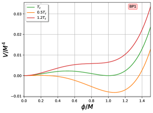
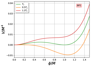
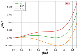
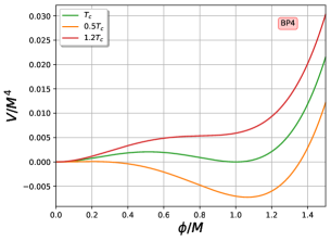
Figure 1: Shape of the potential at, above and below the critical temperature $T_{c}$ for chosen benchmark points shown in Table 1.

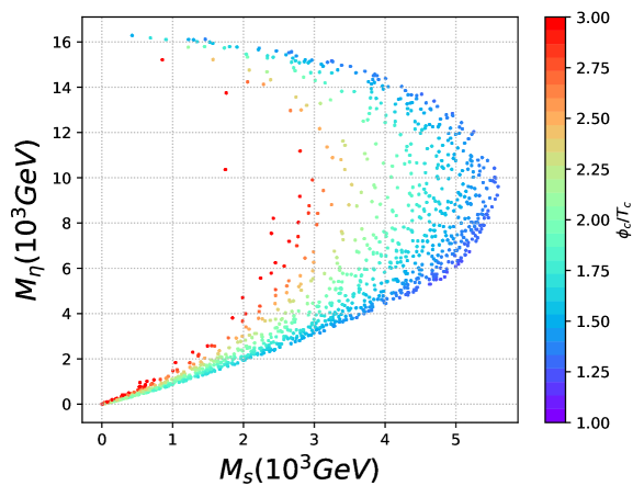
Figure 2: Parameter space in inert doublet Mass $M_{\eta}$ versus scalar singlet mass $M_{S}$ plane consistent with a FOPT in conformal scotogenic model. The colour code indicates the strength of the FOPT.

IV Stochastic Gravitational Waves from FOPT

A FOPT can lead to the formation of stochastic gravitational waves (GW) background primarily due to three distinct mechanisms: the bubble collisions Turner:1990rc ; Kosowsky:1991ua ; Kosowsky:1992rz ; Kosowsky:1992vn ; Turner:1992tz , the sound wave of the plasma Hindmarsh:2013xza ; Giblin:2014qia ; Hindmarsh:2015qta ; Hindmarsh:2017gnf and the turbulence of the plasma Kamionkowski:1993fg ; Kosowsky:2001xp ; Caprini:2006jb ; Gogoberidze:2007an ; Caprini:2009yp ; Niksa:2018ofa . The amplitude of such GW signal crucially depends upon two quantities: the amount of vacuum energy (or latent heat) released during the transition as well as the duration of the transition.

In order to calculate the energy released during the FOPT, we first find the free energy difference between the true and the false vacuum as

$$\Delta V_{\rm tot}\equiv V_{\rm tot}(\phi_{\rm false},T)-V_{\rm tot}(\phi_{\rm true},T).$$ (24)

As a result of the bubble nucleation, the amount of vacuum energy released during the FOPT, in the units of radiation energy density of the universe, $\rho_{\rm rad}=g_{*}\pi^{2}T^{4}/30$, is given by

$$\alpha_{*}=\frac{\epsilon_{*}}{\rho_{\rm rad}},$$ (25)

with

$$\epsilon_{*}=\left[\Delta V_{\rm tot}-\frac{T}{4}\frac{\partial\Delta V_{\rm tot}}{\partial T}\right]_{T=T_{*}},$$ (26)

which is also related to the change in the trace of the energy-momentum tensor across the bubble wall Caprini:2019egz ; Borah:2020wut .

On the other hand, the duration of the FOPT, denoted by the parameter $\beta$, is defined as Caprini:2015zlo

$$\frac{\beta}{{\bf H}(T)}\simeq T\frac{d}{dT}\left(\frac{S_{3}}{T}\right).$$ (27)

Here, $\alpha_{*}$ and $\beta/{\bf H}(T)$ are evaluated at the nucleation temperature $T=T_{*}$ with $S_{3}$ being evaluated using Eq. (17). In order to calculate the action numerically, we use a fit for the actual potential which matches very well with the actual potential, as shown in Appendix B. For the benchmark points discussed earlier, we calculate these key parameters and show them in Table 2 along with other relevant parameters.

	$T_{c}$ (GeV)	$v_{c}/T_{c}$	$T_{n}$ (GeV)	$T_{p}$ (GeV)	$(\beta/{\bf H}_{*})$	$v_{J}$	$\alpha_{*}$
BP1	2374	4.01	810.86	808.35	77.43	0.93	0.99
BP2	2407	3.98	1098.88	1084.30	168.18	0.86	0.35
BP3	2422	4.01	834.79	823.52	125.87	0.91	0.61
BP4	2391	4.03	975.59	962.33	150.66	0.88	0.44

Table 2: Benchmark parameters consistent with FOPT in conformal scotogenic model, along with the FOPT related parameters calculated for GW spectrum estimation.

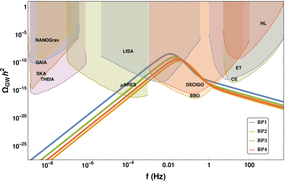
Figure 3: Gravitational wave spectrum from FOPT in conformal scotogenic model for four different benchmark points given in table 2. Different coloured curves show the sensitivities from GW search experiments like LISA, BBO, DECIGO, HL (aLIGO), ET, CE, NANOGrav, SKA, GAIA, THEIA and $\mu$ARES.

Now, considering the three contributions to GW production mentioned above, the corresponding GW power spectrum can be written as Cai:2017tmh

$$\Omega_{\rm GW}(f) =\Omega_{\phi}(f)+\Omega_{\rm sw}(f)+\Omega_{\rm turb}(f).$$ (28)

In general, each of these contributions can be characterised by its own peak frequency and each GW spectrum can be written in parametric form as

$$h^{2}\Omega(f) =\mathcal{R}\Delta(v_{w})\left(\frac{\kappa\alpha_{*}}{1+\alpha_{*}}\right)^{p}\left(\frac{{\bf H_{*}}}{\beta}\right)^{q}\mathcal{S}(f/f_{\rm peak}).$$ (29)

Here, the pre-factor $\mathcal{R}\simeq 7.69\times 10^{-5}g^{-1/3}_{*}$ takes in account the red-shift of the GW energy density, $\mathcal{S}(f/f_{\rm peak})$ parametrises the shape of the spectrum and $\Delta(v_{w})$ is the normalization factor which depends on the bubble wall velocity $v_{w}$. The Hubble parameter at the nucleation temperature $T=T_{n}$ is denoted by ${\bf H_{*}}$. For bubble collision as source, the spectrum can be written as Cai:2017tmh

$$\Omega_{\phi}h^{2}=1.67\times 10^{-5}\left(\frac{100}{g_{*}}\right)^{1/3}\left(\frac{{\bf H_{*}}}{\beta}\right)^{2}\left(\frac{\kappa\alpha_{*}}{1+\alpha_{*}}\right)^{2}\frac{0.11v^{3}_{w}}{0.42+v^{2}_{w}}\frac{3.8(f/f_{\rm peak})^{2.8}}{1+2.8(f/f_{\rm peak})^{3.8}}$$ (30)

with the peak frequency being given by

$$f_{\rm peak}=1.65\times 10^{-5}{\rm Hz}\left(\frac{g_{*}}{100}\right)^{1/6}\left(\frac{T_{n}}{100\;{\rm GeV}}\right)\frac{0.62}{1.8-0.1v_{w}+v^{2}_{w}}\left(\frac{\beta}{{\bf H_{*}}}\right).$$ (31)

Similarly, the other contributions can also be written following Cai:2017tmh and references therein. In order to calculate the bubble wall velocity., we first calculate the Jouguet velocity Kamionkowski:1993fg ; Steinhardt:1981ct ; Espinosa:2010hh :

$$v_{J}=\frac{1/\sqrt{3}+\sqrt{\alpha^{2}_{*}+2\alpha_{*}/3}}{1+\alpha_{*}}.$$ (32)

The bubble wall velocity is then calculated as Lewicki:2021pgr

$$v_{w}=\begin{cases}\sqrt{\frac{\Delta V_{\rm tot}}{\alpha_{*}\rho_{\rm rad}}}&\text{if}\,\,\sqrt{\frac{\Delta V_{\rm tot}}{\alpha_{*}\rho_{\rm rad}}}<v_{J}\\ 1&\text{if}\,\,\sqrt{\frac{\Delta V_{\rm tot}}{\alpha_{*}\rho_{\rm rad}}}\geq v_{J}.\\ \end{cases}$$ (33)

The total GW spectrum after summing over the contributions from all three sources is shown in Fig. 3 for the benchmark points shown in Table 2. The experimental sensitivities of NANOGrav McLaughlin:2013ira , SKA Weltman:2018zrl , GAIA Garcia-Bellido:2021zgu , THEIA Garcia-Bellido:2021zgu , $\mu$ARES Sesana:2019vho , LISA AmaroSeoane2012LaserIS , DECIGO Kawamura:2006up , BBO Yagi:2011wg , ET Punturo_2010 , CE LIGOScientific:2016wof and aLIGO LIGOScientific:2014pky are shown as shaded regions of different colours. Since the FOPT is occurring at a scale above the electroweak scale, the peak frequencies as well as the amplitudes are around the LISA sensitivity and hence remain verifiable in near future.

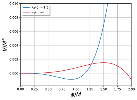
Figure 4: Zero temperature effective potential at one-loop for two different values of singlet-$\eta$ coupling $\lambda_{7}$, considering the singlet-RHN Yukawa coupling $Y^{\prime}(0)=0.8$.

V Dark Matter and Leptogenesis via FOPT

In order to realise leptogenesis from decay, one needs to ensure that at least one of the RHNs remain heavier than the scalar doublet $\eta$. Since both $\eta$ and RHNs acquire masses during the FOPT, this helps in realising DM and leptogenesis simultaneously. However, the desired profile of the scalar potential of singlet scalar $S$ as well as the minimisation condition given in Eq. (22) pose a problem. As understood from the FOPT, the scalar singlet potential has one unique minima $\phi=0$ at very high temperature $T\gg M$ with the effective self-quartic coupling $\lambda_{s}>0$. However, for low temperature $T\ll M$, the self quartic coupling turns negative and $\phi=0$ should become a false vacuum. This is however, not possible unless we have $\lambda^{2}_{7}(0)>3Y^{\prime 2}(0)$. This can be seen from Fig. 4 where the zero-temperature effective potential is shown for two different values of $\lambda_{7}(0)$ while keeping singlet-RHN Yukawa fixed $Y^{\prime}(0)=0.8$. Clearly, for smaller $\lambda_{7}(0)$, we can not achieve the desired potential profile at zero temperature.

In order to circumvent this problem, we consider a hybrid of scotogenic and type I seesaw model without increasing the number of fields. Out of the three RHNs in conformal scotogenic model, we consider two of them to be $Z_{2}$ even such that they couple to the SM lepton doublets via usual Higgs doublet as $y_{D}\overline{L}\tilde{\Phi_{1}}N_{2,3}$. The other RHN namely, $N_{1}$ is $Z_{2}$-odd and couple to the SM lepton doublets via $\eta$ as before. Thus, two of the active neutrinos will receive non-zero mass from type I seesaw while the third one will receive scotogenic contribution at one-loop. The scalar potential as well as singlet scalar coupling to RHNs remain same as before and hence we still require $\eta$ to be heavier than the RHNs. Therefore $N_{1}$ is our DM candidate and $N_{2,3}$ can decay into $L\Phi_{1}$ to generate the required lepton asymmetry.

We first identify a few benchmark points consistent with the FOPT and the mass hierarchy among RHN and scalar doublet $\eta$ required to have successful leptogenesis and DM phenomenology. The benchmark points along with other details calculated for the GW spectrum are shown in table 3. The corresponding GW spectrum is shown in Fig. 5. Clearly, choosing one RHN lighter and making the heavier RHNs $Z_{2}$ even does not change the FOPT details significantly and hence we obtain similar benchmark parameters and GW spectrum like before.

	$v_{c}$	$T_{c}$	v	$v_{c}/T_{c}$	$\lambda_{7}(0)$	$Y^{\prime}_{2}(0)$	$\lambda_{s}(0)$	$T_{n}$	$T_{p}$	$(\beta/{\bf H}_{*})$	$v_{J}$	$\alpha_{*}$
	(GeV)	(GeV)	(GeV)			$\approx Y^{\prime}_{3}(0)$		(GeV)	(GeV)
BP1	9634.17	2521	9934.17	3.82	1.5	0.5	0.02	988.32	974.98	151.06	0.89	0.46
BP2	9553.88	2416	9757.60	3.95	1.6	0.7	0.02	896.89	887.67	110.66	0.91	0.66
BP3	9698.63	2370	9988.01	4.09	1.2	0.3	0.02	779.49	770.72	103.96	0.92	0.80
BP4	9692.84	2391	9978.08	4.05	1.3	0.4	0.02	1207.09	1190.58	204.51	0.84	0.24

Table 3: Benchmark parameters and other details involved in the GW spectrum calculation of the hybrid model.

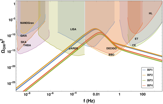
Figure 5: Gravitational wave spectrum from FOPT in the hybrid model for four different benchmark points given in table 3. Different coloured curves show the sensitivities from GW search experiments like LISA, BBO, DECIGO, HL (aLIGO), ET, CE, NANOGrav, SKA, GAIA, THEIA and $\mu$ARES.

Now we implement the baryogenesis via relativistic bubble wall mechanism proposed in Baldes:2021vyz to achieve leptogenesis in the hybrid model mentioned above. A first order phase transition in the singlet (S) sector will create bubbles such that the particles like $N_{i},\eta$ entering the bubble will become massive due to $\langle S\rangle\neq 0$ inside the bubble. This is followed by $N_{2,3}$ decays into leptons and SM Higgs creating the leptonic asymmetry. On the other hand $N_{1}$ being lighter than $\eta$ become stable due to unbroken $Z_{2}$ symmetry and hence act like a DM candidate.

	$\epsilon_{N}$	$T_{\rm RH}$ (GeV)	$T_{n}$ (GeV)	$M_{N_{2}}\approx M_{N_{3}}$ (GeV)	$y_{D}$	$\Delta V_{\rm tot}$ (GeV)4
BP1	$6.22\times 10^{-8}$	988.32	988.32	4966.67	$5.12\times 10^{-8}$	$1.75464\times 10^{13}$
BP2	$6.22\times 10^{-8}$	896.89	896.89	6826.16	$6\times 10^{-8}$	$1.69737\times 10^{13}$
BP3	$6.22\times 10^{-8}$	779.49	779.49	2996.39	$3.98\times 10^{-8}$	$1.15697\times 10^{13}$
BP4	$6.22\times 10^{-8}$	1207.58	1207.58	3991.16	$4.59\times 10^{-8}$	$2.15494\times 10^{13}$

Table 4: CP asymmetry and other relevant details involved in leptogenesis calculation for the hybrid model.

For the leptogenesis we closely follow Ref. Baldes:2021vyz ; Dasgupta:2022isg i.e., the mass -gain mechanism. Let us briefly mention the mass-gain mechanism employed in our work. Firstly, we need to ensure that the Lorentz boost of the bubble wall should be more than the Lorentz factor of the particle in the plasma frame

$$\gamma_{w}>\gamma_{N}\sim\frac{M_{N}}{T_{n}}$$ (34)

where $T_{n}$ is the nucleation temperature and $M_{N}=y_{N}v$ is the mass of the RHN coupling to the singlet scalar. Now, the above condition (34) pushes the RHN into the bubble while maintaining the equilibrium co-moving number density.

$$Y_{N} =\frac{135}{8\pi^{4}}\xi(3)\frac{g_{N}}{g_{*}}$$ (35)

where $g_{N}$ and $g_{*}$ are the degrees of freedom of RHN $N$ and the total relativistic degrees of freedom in the energy density of the universe, respectively.

The final baryonic asymmetry is then written as follows

$$Y_{B} =\epsilon_{N}\kappa_{\rm sph}Y_{N}\left(\frac{T_{n}}{T_{RH}}\right)^{3}.$$ (36)

where $\epsilon_{N}\simeq\sin(2\delta)/(16\pi)$ Pilaftsis:1998pd ; Pilaftsis:2003gt is the CP-asymmetry and $\delta$ is the relative CP phase between the RHNs (for resonant regime), $\kappa_{\rm Sph}=8/23$ is the sphaleron conversion factor in the presence of two Higgs doublets Kuzmin:1985mm , and $T_{\rm RH}$ is the reheating temperature after the FOPT. $T_{\rm RH}$ is defined as $T_{\rm RH}={\rm Max}[T_{n},T_{\rm inf}]$ Baldes:2021vyz where $T_{\rm inf}$ can be obtained from the following relation

$$\frac{g_{*}\pi^{2}}{30}T^{4}_{\rm inf}=\Delta V_{\rm tot}.$$ (37)

Using $\Delta V_{\rm tot}$ for the benchmark parameters given in table 4, we can calculate the corresponding $T_{\rm inf}$ and hence $T_{\rm RH}$. The $Y_{B}$ obtained in Eq. (36) should then be compared with the observed baryon asymmetry normalized over the entropy density: $Y_{B}^{\rm obs}=(8.61\pm 0.05)\times 10^{-11}$ Planck:2018vyg .

The above asymmetry is feasible after satisfying two condition

1. The feasibility of decay $N_{2,3}\rightarrow LH$

2. The wash-out from the dominant inverse decay to be suppressed.

For the first condition we will need to consider the thermally corrected masses for the SM Higgs and lepton doublets at the reheating temperature Giudice:2003jh

$$M_{H}^{2}(T) =\left(\frac{3}{16}g^{2}_{2}+\frac{1}{16}g^{2}_{1}+\frac{1}{4}y^{2}_{t}\right)T^{2}\,,$$

$$M^{2}_{L}(T) =\left(\frac{3}{32}g^{2}_{2}+\frac{1}{32}g^{2}_{1}\right)T^{2}\,,$$ (38)

where $g_{1}$ and $g_{2}$ are the $U(1)_{Y}$ and $SU(2)_{L}$ gauge couplings respectively, and $y_{t}$ is the top quark Yukawa coupling. Therefore, at the reheating temperature after considering the coupling values at the electroweak scale we get

$$M_{H}(T_{\rm RH})+M_{L}(T_{\rm RH}) \simeq 0.77T_{\rm RH},$$ (39)

Hence for the feasibility of the decay we need the mass of RHN at the reheating temperature to be $M_{N}/T_{\rm RH}\gtrsim 0.77$.

As for the second condition we have taken the Dirac Yukawa coupling $y_{D}$, which is responsible for the wash-out, to be parameterized by the Casas-Ibarra parameterization Casas:2001sr for type I seesaw with two RHNs given by

$$Y_{D} =\Lambda^{-1/2}\mathcal{O}\widehat{m}_{\nu}^{1/2}U^{\dagger}_{\rm PMNS}\,,$$ (40)

where $\Lambda=v^{2}_{\rm ew}/M_{N}$, ${\cal O}$ is an arbitrary complex orthogonal matrix, $\widehat{m}_{\nu}$ is the diagonal light neutrino mass matrix and $U_{\rm PMNS}$ is the light neutrino mixing matrix. Since only two RHNs contribute to type I seesaw, we consider the lightest active neutrino mass to be vanishing. Using the best-fit values of the light neutrino oscillation data Gonzalez-Garcia:2021dve for normal hierarchy and assuming ${\cal O}$ to be the identity matrix, we obtain

$$y_{D}\equiv\sum_{\alpha}y_{D_{1\alpha}}\sim 2.3\times 10^{-8}\left(\frac{M_{N}}{1~{}{\rm TeV}}\right)^{1/2}\,.$$ (41)

And proceeding with the above Dirac Yukawa we need to satisfy the following condition Baldes:2021vyz

$$\frac{M_{N}}{T_{\rm RH}}\gtrsim\ln\left[\frac{y_{D}^{2}M_{\rm Pl}}{24\pi T_{\rm RH}}\left(\frac{M_{N}}{T_{\rm RH}}\right)^{5/2}\right],$$ (42)

ensuring the inverse decay width to be suppressed. We calculate the required CP asymmetry and the Dirac Yukawa couplings for the four benchmark points and quote them in table 4. All these benchmark points satisfy the required baryon asymmetry due to the appropriate choice of Yukawa couplings and CP phase. As can be seen from the smallness of the Dirac Yukawa couplings, the decay width of the RHN remains small, also required from the resonant leptogenesis condition $M_{3}-M_{2}\sim\Gamma_{2}/2$. This also justifies the semi-degenerate nature of RHNs $N_{2,3}$ in the benchmark choice of parameters. We also check that the benchmark points satisfy the above mentioned conditions to ensure the viability of the leptogenesis scenario we are implementing.

For the standard vanilla leptogenesis scenario where the massive RHNs are in equilibrium, the baryon asymmetry in the weak washout regime $\Gamma/{\bf H}(T=M_{N})\ll 1$ can be written as

$$Y_{B} =\epsilon_{N}\kappa_{\rm sph}Y^{\rm eq}_{N}(T=M_{N});$$ (43)

$$Y^{\rm eq}_{N}(T) =\frac{45}{4\pi^{4}}\frac{g_{N}}{g_{*}}\left(\frac{M_{N}}{T}\right)^{2}K_{2}(M_{N}/T),$$ (44)

with $K_{2}$ being the modified Bessel function of 2nd order. Comparing with Eq. (36), we can see that in FOPT scenario there arises an extra dilution factor $(T_{n}/T_{\rm RH})^{3}$ compared to the standard case. This was also noticed in earlier works Huang:2022vkf ; Dasgupta:2022isg . However, due to a different structure of our model in the absence of any additional gauge symmetry, we have $T_{\rm inf}<T_{n}$ resulting in $T_{\rm RH}=T_{n}$. Therefore, the final baryon asymmetry in our setup remains same as the standard one, but with the added advantage of detection prospects via stochastic GW observations. In other words, the model without FOPT is also consistent with successful leptogenesis for same set of parameters. However, the presence of FOPT increases the detection prospects in terms of future observations of stochastic GW.

However, as we increase the scale of FOPT, we get deviations from $T_{\rm RH}=T_{n}$ resulting in dilution of lepton asymmetry compared to the standard one. To illustrate this, we show three such benchmark points for high scale leptogenesis in table 5 and 6 which are also consistent with a strong FOPT criteria. As can be seen from table 6, for such high scale FOPT, we have $T_{\rm inf}>T_{n}$ resulting in $T_{\rm RH}>T_{n}$. This leads to the dilution of lepton asymmetry by a factor $(T_{n}/T_{\rm RH})^{3}$ which is as large as $\sim 10^{3}$ for the last benchmark point in table 6. Accordingly, the required CP asymmetry parameter needs to be enhanced for such scenarios. Even though we are in weak washout regime, FOPT can also lead to sizeable washout at the end of the phase transition due to the large latent heat released. Such washout effects can be significant if $T_{\rm RH}\gg M_{N}$. In the benchmark points we have considered, $T_{\rm RH}<M_{N}$ and hence such washout effects are expected to be smaller. Therefore, in the weak washout regime, high scale FOPT scenario can give successful leptogenesis for the parameter space leading to overproduction of asymmetry in standard leptogenesis.

On the other hand, if we are in the strong washout regime of standard leptogenesis, the FOPT triggered leptogenesis can, in principle, enhance the production of asymmetry if the dilution effects are under control and $T_{\rm RH}\ll M_{N}$ in order keep the washout processes like inverse decay suppressed. A detailed investigation of this regime along with implications for dark matter will require the relevant Boltzmann equations to be solved numerically, which we leave for future works.

$v_{c}$	$T_{c}$	v	$v_{c}/T_{c}$	$\lambda_{7}(0)$	$Y^{\prime}_{2}(0)$	$\lambda_{s}(0)$
(GeV)	(GeV)	(GeV)			$\approx Y^{\prime}_{3}(0)$
$9.68\times 10^{7}$	$3.14\times 10^{7}$	$9.93\times 10^{7}$	3.07	2.2	0.6	0.02
$9.52\times 10^{8}$	$2.05\times 10^{8}$	$9.76\times 10^{8}$	4.63	1.2	0.6	0.02
$9.61\times 10^{9}$	$2.62\times 10^{9}$	$9.89\times 10^{9}$	3.66	1.7	0.6	0.02

Table 5: Benchmark parameters and other details for high scale leptogenesis scenario.

$\epsilon_{N}$	$T_{\rm RH}$ (GeV)	$T_{n}$ (GeV)	$M_{N_{2}}\approx M_{N_{3}}$ (GeV)	$y_{D}$	$\Delta V_{\rm tot}$ (GeV)4
$8.93\times 10^{-7}$	$9.87\times 10^{6}$	$4.09\times 10^{6}$	$5.96\times 10^{7}$	$5.62\times 10^{-6}$	$3.62\times 10^{29}$
$1.81\times 10^{-7}$	$7.04\times 10^{7}$	$4.97\times 10^{7}$	$5.85\times 10^{8}$	$1.76\times 10^{-5}$	$9.96\times 10^{32}$
$4.40\times 10^{-5}$	$8.59\times 10^{8}$	$9.71\times 10^{7}$	$5.93\times 10^{9}$	$5.60\times 10^{-5}$	$2.07\times 10^{37}$

Table 6: CP asymmetry and other relevant details involved in high scale leptogenesis calculation for the hybrid model.

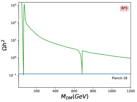
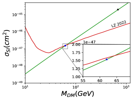
Figure 6: Left panel: WIMP DM relic as a function of its mass for BP3, while considering singlet-SM Higgs mixing to be $\sin{\theta_{hS}}=0.23$. Right panel: Spin-independent DM-nucleon cross-section as a function of DM mass for the same benchmark choices of parameters considered in left panel.

As mentioned earlier, the $Z_{2}$ odd RHN namely, $N_{1}$ is the DM candidate which can have light masses due to its small Yukawa couplings with the singlet scalar. It is possible, in principle, to realise either thermal WIMP or non-thermal DM scenario with the latter being popularly known as feebly interacting massive particle (FIMP) Hall:2009bx . As $M_{\rm DM}<T_{n}$, DM can be in equilibrium inside the bubble and undergo thermal freeze-out at a temperature $T_{f}\sim M_{\rm DM}/20$, if its coupling to the SM bath is sizeable enough. DM can annihilate into SM particles via two possible processes: Yukawa interactions with SM leptons via inert scalar doublet $\eta$ and singlet scalar mediated annihilations into SM particles via singlet-Higgs mixing. Since the scalar doublet $\eta$ is much heavier than the RHNs, the corresponding DM annihilation cross-section remains suppressed compared to the singlet scalar mediated one. Since the singlet scalar mass is small, we can get the desired relic of DM by appropriate tuning of singlet-Higgs mixing. In order to calculate the thermally averaged annihilation cross-sections and solve the Boltzmann equation for DM numerically, we use micrOMEGAs Belanger:2014vza . We consider one particular benchmark point namely, BP3 such that the singlet scalar mass is fixed. The relic abundance as a function of DM mass is shown on the left panel of Fig. 6. Even for a considerably large mixing between singlet scalar and the SM Higgs $\sin{\theta_{hS}}=0.23$, the relic can barely be satisfied at the resonances. Similarly, the stringent direct detection bounds LUX-ZEPLIN:2022qhg barely allows the relic satisfying point at the SM Higgs resonance while ruling out the heavier DM mass at singlet scalar resonance. This is due to the fact that, DM Yukawa coupling with singlet scalar is $\langle S\rangle/M_{\rm DM}=v/m_{N1}$ which is very small for this mass range. It should also be noted that the actual singlet-SM Higgs mixing will be $\sin{\theta_{hS}}\sim\lambda_{6}v_{\rm ew}/v\ll 0.23$ thereby ruling out the WIMP possibility in this minimal setup.

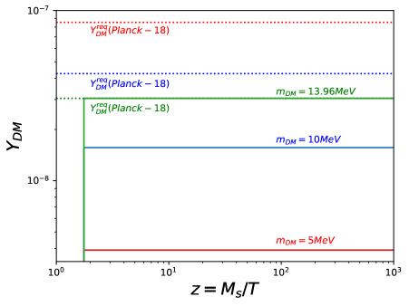
Figure 7: Comoving density of FIMP DM for BP3

We finally consider the FIMP DM possibility by considering singlet scalar decay after the phase transition. The corresponding Boltzmann equations can be written as

$$\frac{dY_{DM}}{dz}=\frac{2}{z\bf{H}}\Gamma_{sN1}Y_{s},\,\,\frac{dY_{s}}{dz}=-\frac{1}{z\bf{H}}(\Gamma_{sN1}+\Gamma_{sh})Y_{s},$$ (45)

with $z=M_{s}/T$ and assuming the relativistic dof to be constant, which is valid at temperatures above electroweak scale. While DM is produced only from the decay of singlet scalar, the latter can decay into SM Higgs as well. The corresponding decay widths are

$$\Gamma_{sN1}=\frac{1}{16\pi}y_{1}^{2}M_{s}\left(1-\frac{4M_{DM}^{2}}{M_{s}^{2}}\right)^{3/2},\,\,\Gamma_{sh}=\frac{y_{shh}^{2}}{16\pi M_{s}}\left(1-\frac{4M_{h}^{2}}{M_{s}^{2}}\right)^{1/2},$$ (46)

where $y_{shh}\sim\lambda_{6}v$. Similar to the case of heavy RHNs $N_{2,3}$, the singlet scalar also acquires a large abundance inside the bubble at nucleation temperature, close to the equilibrium comoving number density without Boltzmann suppression. Considering this to be the initial comoving abundance of S and taking appropriate partial decay width of S into SM Higgs, we solve the above Boltzmann equations for different DM masses and find that for DM mass around 14 MeV, the correct relic is satisfied if other parameters are fixed as in BP3 discussed before. Since singlet decay width into SM Higgs is substantial, we require somewhat large FIMP mass to satisfy the correct DM relic. This also leads to instantaneous freeze-in shortly after nucleation temperature $T\sim T_{*}$ as larger mass corresponds to larger Yukawa coupling of DM with singlet.

VI Conclusion

We have studied the possibility of getting dark matter and low scale leptogenesis from a supercooled first order phase transition driven by a singlet scalar around TeV scale. The right handed neutrinos responsible for generating lepton asymmetry via decay and dark matter acquire masses by crossing the relativistic bubble walls which arise as a result of the FOPT. This also leads to a large abundance of RHN in true vacuum inside the bubble sufficient for generating the required lepton asymmetry without washout or Boltzmann suppression. The dark matter is lighter than the nucleation temperature and hence can remain in equilibrium inside the bubble with its relic determined by thermal freeze-out at later stages. In order to implement the idea, we first consider a conformal version of the scotogenic model such that along with dark matter and right handed neutrino generating radiative light neutrino masses, we also have a strong supercooling to bring the resulting gravitational wave amplitude within near future experiment’s sensitivity. While a strong supercooled FOPT is possible, the hierarchy of the additional field content of the model does not allow the realisation of leptogenesis from RHN decay. We then consider a hybrid scenario with the same field content but different seesaw realisation to show correct DM phenomenology from the lightest RHN while the heavier two RHNs can lead to successful TeV scale resonant leptogenesis. The light neutrino mass arises from a hybrid seesaw mechanism involving both type I and radiative origin. As the FOPT details remain more or less similar to the conformal scotogenic model, we can probe this hybrid model in near future GW experiments like the LISA experiment. Due to TeV scale RHN and additional scalars, the model can also have complementary detection prospects at intensity and energy frontier experiments.

Appendix A Renormalisation Group Evolution Equations

The relevant RGE equations for the model parameters are Bhattacharya:2019tqq

$$\frac{d\lambda_{s}}{dt}=\frac{1}{16\pi^{2}}(20\lambda_{s}^{2}+2\lambda_{6}^{2}+2\lambda_{7}^{2}+8\lambda_{s}{\rm Tr}[Y^{\prime\dagger}Y^{\prime}]-{\rm Tr}[Y^{\prime\dagger}Y^{\prime}Y^{\prime\dagger}Y^{\prime}])$$

$$\frac{d\lambda_{2}}{dt}=\frac{1}{16\pi^{2}}(12\lambda_{2}^{2}+2\lambda_{7}^{2}+3g_{1}^{2}/4+9g_{2}^{2}/4+3g_{1}^{2}g_{2}^{2}/2)$$

$$\frac{d\lambda_{7}}{dt}=\frac{1}{16\pi^{2}}(4\lambda_{7}^{2}+6\lambda_{2}\lambda_{7}+8\lambda_{s}\lambda_{7}+4\lambda_{7}{\rm Tr}[Y^{\prime\dagger}Y^{\prime}])$$

$$\frac{d\lambda_{6}}{dt}=\frac{1}{16\pi^{2}}(4\lambda_{6}^{2}+6\lambda_{6}y_{t}^{2}+8\lambda_{s}\lambda_{6}+4\lambda_{6}{\rm Tr}[Y^{\prime\dagger}Y^{\prime}])$$

$$\frac{dY^{\prime}}{dt}=\frac{1}{16\pi^{2}}(4Y^{\prime 3}+2Y^{\prime}{\rm Tr}[Y^{\prime\dagger}Y^{\prime}])$$

$$\frac{dg_{1}}{dt}=\frac{1}{16\pi^{2}}(7g_{1}^{3})$$

$$\frac{dg_{2}}{dt}=\frac{1}{16\pi^{2}}(-3g_{2}^{3})$$

$$\frac{dy_{t}}{dt}=\frac{1}{16\pi^{2}}(9y_{t}^{3}/2-y_{t}(17g_{1}^{2}/12+9g_{2}^{2}/4))$$

Appendix B Fitting of the finite temperature potential

The generic form of quartic and logarithmic potential can be written asAdams:1993zs

$$V(\phi)=(2A-B)\sigma^{2}\phi^{2}-A\phi^{4}+B\phi^{4}\ln{\frac{\phi^{2}}{\sigma^{2}}}$$ (47)

The above expression as the effective potential can be used to calculate the semi-analytical expression of the Euclidean action in terms of the parameters of the potential. We can use the effective potential with consideration of the running coupling effect, one-loop thermal contribution, and Daisy corrections, which can then be fitted well to the generic potential as shown in Fig. 8 for BP1.

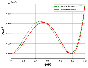
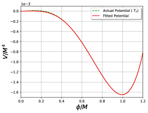
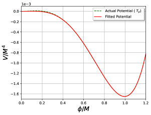
Figure 8: Comparison between the actual thermal potential and the fit at different temperatures.

The bounce equation of motion for the above generic potential in three dimensions is

$$\frac{d^{2}\phi}{dr^{2}}+\frac{2}{r}\frac{d\phi}{dr}=\frac{dV}{d\phi}$$ (48)

We obtain the derivative of the potential as

$$\frac{dV}{d\phi}=4B\sigma^{3}\Bigl{\{}\frac{2A-B}{2B}\Bigl{(}\frac{\phi}{\sigma}-\frac{\phi^{3}}{\sigma^{3}}\Bigl{)}+\frac{\phi^{3}}{\sigma^{3}}\ln{\frac{\phi^{2}}{\sigma^{2}}}\Bigl{\}}$$ (49)

Now using a scaling transformation ($\Phi=\phi/\sigma,\xi=2\sigma\sqrt{B}r$), we reduce the three parameters differential equation (DE) to one parameter DE given by

$$\frac{d^{2}\Phi}{d\xi^{2}}+\frac{2}{\xi}\frac{d\Phi}{d\xi}=\delta(\Phi-\Phi^{3})+\Phi^{3}\ln{\Phi^{2}}$$ (50)

where $\delta=\frac{2A-B}{2B}$. Following the approach of Adams:1993zs , the action in three dimensions, calculated in a semi-analytical manner, is found to be

$$S_{3}=\frac{16\pi\sigma I^{3}}{3(1-2\delta)^{2}}\Bigl{(}\frac{2}{B}\Bigl{)}^{1/2}(2\delta)^{n_{\mu}}\Bigl{\{}1+\mu_{1}\delta+\mu_{2}\delta^{2}+\mu_{3}\delta^{3}\Bigl{\}}$$ (51)

where, I=0.4199, $n_{\mu}=0.557$, $\mu_{1}=4.2719$, $\mu_{2}=-14.5908$ and $\mu_{3}=12.0940$. We have used it in our numerical analysis.

References

- (1) Planck collaboration, Planck 2018 results. VI. Cosmological parameters, 1807.06209.
- (2) Particle Data Group collaboration, Review of Particle Physics, PTEP 2020 (2020) 083C01.
- (3) A. D. Sakharov, Violation of CP Invariance, C asymmetry, and baryon asymmetry of the universe, Pisma Zh. Eksp. Teor. Fiz. 5 (1967) 32.
- (4) S. Weinberg, Cosmological Production of Baryons, Phys. Rev. Lett. 42 (1979) 850.
- (5) E. W. Kolb and S. Wolfram, Baryon Number Generation in the Early Universe, Nucl. Phys. B172 (1980) 224.
- (6) M. Fukugita and T. Yanagida, Baryogenesis Without Grand Unification, Phys. Lett. B174 (1986) 45.
- (7) V. A. Kuzmin, V. A. Rubakov and M. E. Shaposhnikov, On the Anomalous Electroweak Baryon Number Nonconservation in the Early Universe, Phys. Lett. 155B (1985) 36.
- (8) S. Davidson and A. Ibarra, A Lower bound on the right-handed neutrino mass from leptogenesis, Phys. Lett. B535 (2002) 25 [hep-ph/0202239].
- (9) E. K. Akhmedov, V. A. Rubakov and A. Y. Smirnov, Baryogenesis via neutrino oscillations, Phys. Rev. Lett. 81 (1998) 1359 [hep-ph/9803255].
- (10) T. Asaka and M. Shaposhnikov, The MSM, dark matter and baryon asymmetry of the universe, Phys. Lett. B 620 (2005) 17 [hep-ph/0505013].
- (11) A. Abada, G. Arcadi, V. Domcke, M. Drewes, J. Klaric and M. Lucente, Low-scale leptogenesis with three heavy neutrinos, JHEP 01 (2019) 164 [1810.12463].
- (12) M. Drewes, Y. Georis and J. Klarić, Mapping the Viable Parameter Space for Testable Leptogenesis, Phys. Rev. Lett. 128 (2022) 051801 [2106.16226].
- (13) M. Le Dall and A. Ritz, Leptogenesis and the Higgs Portal, Phys. Rev. D 90 (2014) 096002 [1408.2498].
- (14) T. Alanne, T. Hugle, M. Platscher and K. Schmitz, Low-scale leptogenesis assisted by a real scalar singlet, JCAP 03 (2019) 037 [1812.04421].
- (15) T. Hambye, F. S. Ling, L. Lopez Honorez and J. Rocher, Scalar Multiplet Dark Matter, JHEP 07 (2009) 090 [0903.4010].
- (16) J. Racker, Mass bounds for baryogenesis from particle decays and the inert doublet model, JCAP 03 (2014) 025 [1308.1840].
- (17) J. D. Clarke, R. Foot and R. R. Volkas, Natural leptogenesis and neutrino masses with two Higgs doublets, Phys. Rev. D 92 (2015) 033006 [1505.05744].
- (18) T. Hugle, M. Platscher and K. Schmitz, Low-Scale Leptogenesis in the Scotogenic Neutrino Mass Model, Phys. Rev. D 98 (2018) 023020 [1804.09660].
- (19) D. Borah, P. S. B. Dev and A. Kumar, TeV scale leptogenesis, inflaton dark matter and neutrino mass in a scotogenic model, Phys. Rev. D 99 (2019) 055012 [1810.03645].
- (20) D. Mahanta and D. Borah, Fermion dark matter with leptogenesis in minimal scotogenic model, JCAP 11 (2019) 021 [1906.03577].
- (21) D. Mahanta and D. Borah, TeV Scale Leptogenesis with Dark Matter in Non-standard Cosmology, JCAP 04 (2020) 032 [1912.09726].
- (22) L. Sarma, P. Das and M. K. Das, Scalar dark matter and leptogenesis in the minimal scotogenic model, Nucl. Phys. B 963 (2021) 115300 [2004.13762].
- (23) D. Borah, A. Dasgupta and D. Mahanta, Dark sector assisted low scale leptogenesis from three body decay, Phys. Rev. D 105 (2022) 015015 [2008.10627].
- (24) A. Pilaftsis, Heavy Majorana neutrinos and baryogenesis, Int. J. Mod. Phys. A 14 (1999) 1811 [hep-ph/9812256].
- (25) A. Pilaftsis and T. E. J. Underwood, Resonant leptogenesis, Nucl. Phys. B692 (2004) 303 [hep-ph/0309342].
- (26) E. J. Chun et al., Probing Leptogenesis, Int. J. Mod. Phys. A 33 (2018) 1842005 [1711.02865].
- (27) J. A. Dror, T. Hiramatsu, K. Kohri, H. Murayama and G. White, Testing the Seesaw Mechanism and Leptogenesis with Gravitational Waves, Phys. Rev. Lett. 124 (2020) 041804 [1908.03227].
- (28) S. Blasi, V. Brdar and K. Schmitz, Fingerprint of low-scale leptogenesis in the primordial gravitational-wave spectrum, Phys. Rev. Res. 2 (2020) 043321 [2004.02889].
- (29) B. Fornal and B. Shams Es Haghi, Baryon and Lepton Number Violation from Gravitational Waves, Phys. Rev. D 102 (2020) 115037 [2008.05111].
- (30) R. Samanta and S. Datta, Gravitational wave complementarity and impact of NANOGrav data on gravitational leptogenesis: cosmic strings, 2009.13452.
- (31) B. Barman, D. Borah, A. Dasgupta and A. Ghoshal, Probing high scale Dirac leptogenesis via gravitational waves from domain walls, Phys. Rev. D 106 (2022) 015007 [2205.03422].
- (32) I. Baldes, S. Blasi, A. Mariotti, A. Sevrin and K. Turbang, Baryogenesis via relativistic bubble expansion, Phys. Rev. D 104 (2021) 115029 [2106.15602].
- (33) A. Azatov, M. Vanvlasselaer and W. Yin, Baryogenesis via relativistic bubble walls, JHEP 10 (2021) 043 [2106.14913].
- (34) P. Huang and K.-P. Xie, Leptogenesis triggered by a first-order phase transition, 2206.04691.
- (35) A. Dasgupta, P. S. B. Dev, A. Ghoshal and A. Mazumdar, Gravitational Wave Pathway to Testable Leptogenesis, 2206.07032.
- (36) C. Yuan, R. Brito and V. Cardoso, Probing ultralight dark matter with future ground-based gravitational-wave detectors, Phys. Rev. D 104 (2021) 044011 [2106.00021].
- (37) L. Tsukada, R. Brito, W. E. East and N. Siemonsen, Modeling and searching for a stochastic gravitational-wave background from ultralight vector bosons, Phys. Rev. D 103 (2021) 083005 [2011.06995].
- (38) A. Chatrchyan and J. Jaeckel, Gravitational waves from the fragmentation of axion-like particle dark matter, JCAP 02 (2021) 003 [2004.07844].
- (39) L. Bian, X. Liu and K.-P. Xie, Probing superheavy dark matter with gravitational waves, JHEP 11 (2021) 175 [2107.13112].
- (40) R. Samanta and F. R. Urban, Testing Super Heavy Dark Matter from Primordial Black Holes with Gravitational Waves, 2112.04836.
- (41) D. Borah, S. J. Das, A. K. Saha and R. Samanta, Probing Miracle-less WIMP Dark Matter via Gravitational Waves Spectral Shapes, 2202.10474.
- (42) A. Azatov, M. Vanvlasselaer and W. Yin, Dark Matter production from relativistic bubble walls, JHEP 03 (2021) 288 [2101.05721].
- (43) A. Azatov, G. Barni, S. Chakraborty, M. Vanvlasselaer and W. Yin, Ultra-relativistic bubbles from the simplest Higgs portal and their cosmological consequences, 2207.02230.
- (44) I. Baldes, Y. Gouttenoire and F. Sala, Hot and Heavy Dark Matter from Supercooling, 2207.05096.
- (45) LUX-ZEPLIN collaboration, First Dark Matter Search Results from the LUX-ZEPLIN (LZ) Experiment, 2207.03764.
- (46) J. Arakawa, A. Rajaraman and T. M. P. Tait, Annihilogenesis, JHEP 08 (2022) 078 [2109.13941].
- (47) M. Ahmadvand, Filtered asymmetric dark matter during the Peccei-Quinn phase transition, JHEP 10 (2021) 109 [2108.00958].
- (48) E. Ma, Verifiable radiative seesaw mechanism of neutrino mass and dark matter, Phys. Rev. D 73 (2006) 077301 [hep-ph/0601225].
- (49) A. Ahriche, K. L. McDonald and S. Nasri, The Scale-Invariant Scotogenic Model, JHEP 06 (2016) 182 [1604.05569].
- (50) A. Merle and M. Platscher, Running of radiative neutrino masses: the scotogenic model — revisited, JHEP 11 (2015) 148 [1507.06314].
- (51) D. Borah, A. Dasgupta, K. Fujikura, S. K. Kang and D. Mahanta, Observable Gravitational Waves in Minimal Scotogenic Model, JCAP 08 (2020) 046 [2003.02276].
- (52) L. Dolan and R. Jackiw, Symmetry Behavior at Finite Temperature, Phys. Rev. D 9 (1974) 3320.
- (53) M. Quiros, Finite temperature field theory and phase transitions, in ICTP Summer School in High-Energy Physics and Cosmology, pp. 187–259, 1, 1999, hep-ph/9901312.
- (54) C. Wainwright, S. Profumo and M. J. Ramsey-Musolf, Gravity Waves from a Cosmological Phase Transition: Gauge Artifacts and Daisy Resummations, Phys. Rev. D 84 (2011) 023521 [1104.5487].
- (55) C. L. Wainwright, S. Profumo and M. J. Ramsey-Musolf, Phase Transitions and Gauge Artifacts in an Abelian Higgs Plus Singlet Model, Phys. Rev. D 86 (2012) 083537 [1204.5464].
- (56) S. R. Coleman and E. J. Weinberg, Radiative Corrections as the Origin of Spontaneous Symmetry Breaking, Phys. Rev. D 7 (1973) 1888.
- (57) P. Fendley, The Effective Potential and the Coupling Constant at High Temperature, Phys. Lett. B 196 (1987) 175.
- (58) R. R. Parwani, Resummation in a hot scalar field theory, Phys. Rev. D 45 (1992) 4695 [hep-ph/9204216].
- (59) P. B. Arnold and O. Espinosa, The Effective potential and first order phase transitions: Beyond leading-order, Phys. Rev. D 47 (1993) 3546 [hep-ph/9212235].
- (60) J. M. Cline, M. Jarvinen and F. Sannino, The Electroweak Phase Transition in Nearly Conformal Technicolor, Phys. Rev. D 78 (2008) 075027 [0808.1512].
- (61) A. Mazumdar and G. White, Review of cosmic phase transitions: their significance and experimental signatures, Rept. Prog. Phys. 82 (2019) 076901 [1811.01948].
- (62) M. B. Hindmarsh, M. Lüben, J. Lumma and M. Pauly, Phase transitions in the early universe, SciPost Phys. Lect. Notes 24 (2021) 1 [2008.09136].
- (63) A. D. Linde, Fate of the False Vacuum at Finite Temperature: Theory and Applications, Phys. Lett. B 100 (1981) 37.
- (64) R. Jinno and M. Takimoto, Probing a classically conformal B-L model with gravitational waves, Phys. Rev. D 95 (2017) 015020 [1604.05035].
- (65) S. Iso, N. Okada and Y. Orikasa, The minimal B-L model naturally realized at TeV scale, Phys. Rev. D 80 (2009) 115007 [0909.0128].
- (66) J. Ellis, M. Lewicki and J. M. No, On the Maximal Strength of a First-Order Electroweak Phase Transition and its Gravitational Wave Signal, 1809.08242.
- (67) J. Ellis, M. Lewicki and V. Vaskonen, Updated predictions for gravitational waves produced in a strongly supercooled phase transition, JCAP 11 (2020) 020 [2007.15586].
- (68) P. Athron, C. Balázs, A. Fowlie and Y. Zhang, PhaseTracer: tracing cosmological phases and calculating transition properties, Eur. Phys. J. C 80 (2020) 567 [2003.02859].
- (69) M. S. Turner and F. Wilczek, Relic gravitational waves and extended inflation, Phys. Rev. Lett. 65 (1990) 3080.
- (70) A. Kosowsky, M. S. Turner and R. Watkins, Gravitational radiation from colliding vacuum bubbles, Phys. Rev. D 45 (1992) 4514.
- (71) A. Kosowsky, M. S. Turner and R. Watkins, Gravitational waves from first order cosmological phase transitions, Phys. Rev. Lett. 69 (1992) 2026.
- (72) A. Kosowsky and M. S. Turner, Gravitational radiation from colliding vacuum bubbles: envelope approximation to many bubble collisions, Phys. Rev. D 47 (1993) 4372 [astro-ph/9211004].
- (73) M. S. Turner, E. J. Weinberg and L. M. Widrow, Bubble nucleation in first order inflation and other cosmological phase transitions, Phys. Rev. D 46 (1992) 2384.
- (74) M. Hindmarsh, S. J. Huber, K. Rummukainen and D. J. Weir, Gravitational waves from the sound of a first order phase transition, Phys. Rev. Lett. 112 (2014) 041301 [1304.2433].
- (75) J. T. Giblin and J. B. Mertens, Gravitional radiation from first-order phase transitions in the presence of a fluid, Phys. Rev. D 90 (2014) 023532 [1405.4005].
- (76) M. Hindmarsh, S. J. Huber, K. Rummukainen and D. J. Weir, Numerical simulations of acoustically generated gravitational waves at a first order phase transition, Phys. Rev. D 92 (2015) 123009 [1504.03291].
- (77) M. Hindmarsh, S. J. Huber, K. Rummukainen and D. J. Weir, Shape of the acoustic gravitational wave power spectrum from a first order phase transition, Phys. Rev. D 96 (2017) 103520 [1704.05871].
- (78) M. Kamionkowski, A. Kosowsky and M. S. Turner, Gravitational radiation from first order phase transitions, Phys. Rev. D 49 (1994) 2837 [astro-ph/9310044].
- (79) A. Kosowsky, A. Mack and T. Kahniashvili, Gravitational radiation from cosmological turbulence, Phys. Rev. D 66 (2002) 024030 [astro-ph/0111483].
- (80) C. Caprini and R. Durrer, Gravitational waves from stochastic relativistic sources: Primordial turbulence and magnetic fields, Phys. Rev. D74 (2006) 063521 [astro-ph/0603476].
- (81) G. Gogoberidze, T. Kahniashvili and A. Kosowsky, The Spectrum of Gravitational Radiation from Primordial Turbulence, Phys. Rev. D 76 (2007) 083002 [0705.1733].
- (82) C. Caprini, R. Durrer and G. Servant, The stochastic gravitational wave background from turbulence and magnetic fields generated by a first-order phase transition, JCAP 0912 (2009) 024 [0909.0622].
- (83) P. Niksa, M. Schlederer and G. Sigl, Gravitational Waves produced by Compressible MHD Turbulence from Cosmological Phase Transitions, Class. Quant. Grav. 35 (2018) 144001 [1803.02271].
- (84) C. Caprini et al., Detecting gravitational waves from cosmological phase transitions with LISA: an update, JCAP 03 (2020) 024 [1910.13125].
- (85) C. Caprini et al., Science with the space-based interferometer eLISA. II: Gravitational waves from cosmological phase transitions, JCAP 1604 (2016) 001 [1512.06239].
- (86) R.-G. Cai, M. Sasaki and S.-J. Wang, The gravitational waves from the first-order phase transition with a dimension-six operator, JCAP 08 (2017) 004 [1707.03001].
- (87) P. J. Steinhardt, Relativistic Detonation Waves and Bubble Growth in False Vacuum Decay, Phys. Rev. D25 (1982) 2074.
- (88) J. R. Espinosa, T. Konstandin, J. M. No and G. Servant, Energy Budget of Cosmological First-order Phase Transitions, JCAP 06 (2010) 028 [1004.4187].
- (89) S. J. Huber and M. Sopena, An efficient approach to electroweak bubble velocities, 1302.1044.
- (90) L. Leitao and A. Megevand, Hydrodynamics of phase transition fronts and the speed of sound in the plasma, Nucl. Phys. B 891 (2015) 159 [1410.3875].
- (91) G. C. Dorsch, S. J. Huber and T. Konstandin, Bubble wall velocities in the Standard Model and beyond, JCAP 12 (2018) 034 [1809.04907].
- (92) J. M. Cline and K. Kainulainen, Electroweak baryogenesis at high bubble wall velocities, Phys. Rev. D 101 (2020) 063525 [2001.00568].
- (93) M. Lewicki, M. Merchand and M. Zych, Electroweak bubble wall expansion: gravitational waves and baryogenesis in Standard Model-like thermal plasma, JHEP 02 (2022) 017 [2111.02393].
- (94) M. A. McLaughlin, The North American Nanohertz Observatory for Gravitational Waves, Class. Quant. Grav. 30 (2013) 224008 [1310.0758].
- (95) A. Weltman et al., Fundamental physics with the Square Kilometre Array, Publ. Astron. Soc. Austral. 37 (2020) e002 [1810.02680].
- (96) J. Garcia-Bellido, H. Murayama and G. White, Exploring the Early Universe with Gaia and THEIA, 2104.04778.
- (97) A. Sesana et al., Unveiling the gravitational universe at -Hz frequencies, Exper. Astron. 51 (2021) 1333 [1908.11391].
- (98) P. Amaro-Seoane, H. Audley, S. Babak, J. M. Baker, E. Barausse, P. L. Bender et al., Laser interferometer space antenna, 2012.
- (99) S. Kawamura et al., The Japanese space gravitational wave antenna DECIGO, Class. Quant. Grav. 23 (2006) S125.
- (100) K. Yagi and N. Seto, Detector configuration of DECIGO/BBO and identification of cosmological neutron-star binaries, Phys. Rev. D 83 (2011) 044011 [1101.3940].
- (101) M. Punturo, M. Abernathy, F. Acernese, B. Allen, N. Andersson, K. Arun et al., The einstein telescope: a third-generation gravitational wave observatory, Classical and Quantum Gravity 27 (2010) 194002.
- (102) LIGO Scientific collaboration, Exploring the Sensitivity of Next Generation Gravitational Wave Detectors, Class. Quant. Grav. 34 (2017) 044001 [1607.08697].
- (103) LIGO Scientific collaboration, Advanced LIGO, Class. Quant. Grav. 32 (2015) 074001 [1411.4547].
- (104) Planck collaboration, Planck 2018 results. VI. Cosmological parameters, Astron. Astrophys. 641 (2020) A6 [1807.06209].
- (105) G. Giudice, A. Notari, M. Raidal, A. Riotto and A. Strumia, Towards a complete theory of thermal leptogenesis in the SM and MSSM, Nucl. Phys. B 685 (2004) 89 [hep-ph/0310123].
- (106) J. A. Casas and A. Ibarra, Oscillating neutrinos and , Nucl. Phys. B 618 (2001) 171 [hep-ph/0103065].
- (107) M. C. Gonzalez-Garcia, M. Maltoni and T. Schwetz, NuFIT: Three-Flavour Global Analyses of Neutrino Oscillation Experiments, Universe 7 (2021) 459 [2111.03086].
- (108) L. J. Hall, K. Jedamzik, J. March-Russell and S. M. West, Freeze-In Production of FIMP Dark Matter, JHEP 03 (2010) 080 [0911.1120].
- (109) G. Bélanger, F. Boudjema, A. Pukhov and A. Semenov, micrOMEGAs4.1: two dark matter candidates, Comput. Phys. Commun. 192 (2015) 322 [1407.6129].
- (110) S. Bhattacharya, N. Chakrabarty, R. Roshan and A. Sil, Multicomponent dark matter in extended : neutrino mass and high scale validity, 1910.00612.
- (111) F. C. Adams, General solutions for tunneling of scalar fields with quartic potentials, Phys. Rev. D 48 (1993) 2800 [hep-ph/9302321].