Absence of thermalization in an interacting system of thousands of quantum spins

Abstract

Understanding how closed quantum systems dynamically approach thermal equilibrium presents a major unresolved problem in statistical physics. Generically, it is expected that non-integrable quantum systems thermalize as they comply with the Eigenstate Thermalization Hypothesis (ETH) [1, 2, 3]. A notable exception to this is the phenomenon of many-body localization [4, 5], where the emergence of local conserved quantities prevents thermalization, which has been observed in finite low-dimensional systems. We study an ensemble of Heisenberg spins with a tunable distribution of random coupling strengths realized by a Rydberg quantum simulator [6]. The total magnetization as a function of external field after a quench [7, 8] serves as a probe for thermalization. We find that such an isolated quantum system exhibits a non-thermalizing regime despite being non-integrable. It is shown that thermalization can be restored by reducing the disorder in the coupling strengths. As our system consists of up to 4000 spins, we thus show that closed quantum systems can fail to reach thermal equilibrium even at system sizes approaching the thermodynamic limit.

The success and accuracy of statistical mechanics to describe nature rests on the assumption that macroscopic systems quickly relax to thermal equilibrium. This complies with our everyday experience: The ripples on a pond caused by a rock being thrown into it disappear quickly leaving a calm surface. This apparent irreversibility of the macroscopic dynamics, despite the reversible laws describing the microscopic dynamics of the water molecules, is explained through the notion of typicality: Macroscopic observables, like the water flow at a specific point, take the same "typical" value for almost all allowed microstates of the system. Therefore, a system prepared in an atypical state will generically evolve into a typical state just because anything else is extremely unlikely. This notion is also expected to apply to quantum systems, where the microstates of the system are the eigenstates of the Hamiltonian operator. In this case, typicality means that local observables take the same values for all eigenstates consistent with dynamic constraints such as energy conservation [9]. As a result, local observables will generically relax towards equilibrium values which agree with a thermal ensemble description. This mechanism for quantum thermalization has been formalized through the ETH [1, 2, 3].

Notably, in disordered systems, the emergence of an extensive number of local conservation laws can invalidate the typicality assumption. As a consequence, quantum thermalization is absent even at infinite times as evidenced by the phenomenon of MBL [4, 5]. While this mechanism is firmly established for finite one-dimensional systems with disorder in external fields, the possibility of the absence of thermalization in systems approaching thermodynamic limit has been questioned [10, 11, 12]. In addition, many open questions remain about the possibility of violating ETH in higher dimensional systems [10, 13, 14, 15, 11] and for off-diagonal disorder [16, 17, 18].

This lack of understanding is rooted in the hardness of solving the out-of-equilibrium dynamics of strongly interacting quantum systems numerically on classical devices and in the scarcity of controlled perturbative approaches. Numerical exact diagonalization is limited to small system sizes of a few tens of particles where finite-size effects strongly affect the study of quantum thermalization [19]. Analytical treatments rely on phenomenological renormalization group approaches which involve uncontrolled approximations [20, 21, 22, 23]. Quantum simulation experiments, fully controlled model systems that can be implemented, e.g. in cold atomic gases [24, 25, 26, 27, 6], may help to overcome this problem. In these experiments, spatially resolved measurements can reveal the absence of transport and thereby demonstrate the failure of thermalization [28, 29, 30, 31]. As a microscopic probe of thermalization, recent works have focused on the direct detection of entanglement entropy [32, 33, 34]. However, relying on full microscopic resolution, again, limits the scalability of these quantum simulations.

In the present work, we show that the absence of thermalization can be probed without the requirement for spatial resolution through macroscopic observables, allowing to scale up accessible system sizes. Specifically, we show that the late-time global magnetization reveals localization effects in a strongly interacting Heisenberg spin-system with transverse field and disordered coupling constants. We find through numerical simulations that the system equilibrates to a steady-state characterized by a sharp cusp at small transverse field, not present in a thermal description of the system. We confirm the persistence of these features in the large system limit through a quantum simulation experiment realizing a Heisenberg spin system in a 3D cloud of thousands of Rydberg atoms. By imposing correlations on the coupling constants, we observe that thermalization is reestablished.

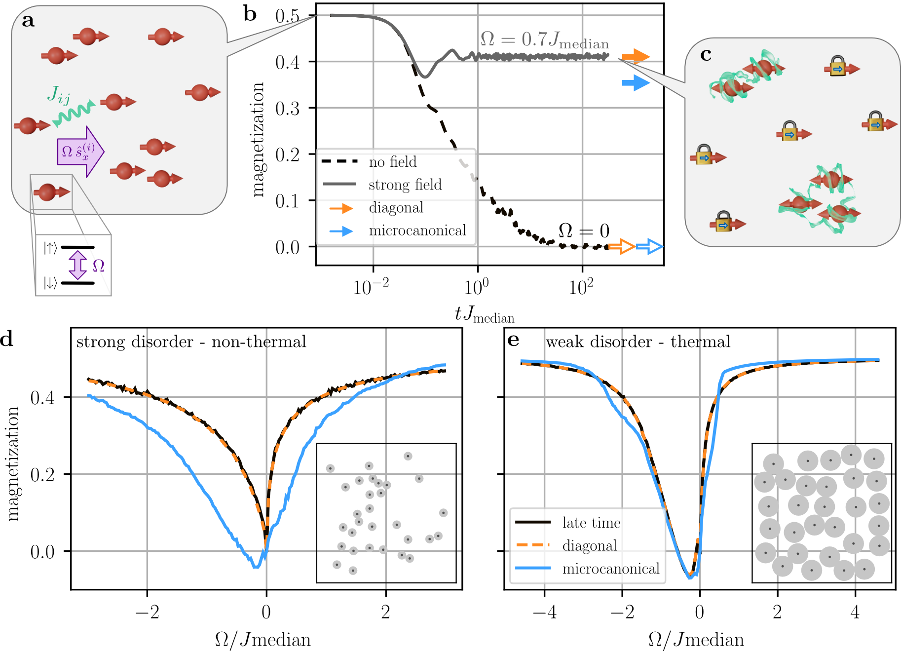
Figure 1: Heisenberg spin systems in transverse fields. a, Schematic illustration of the disordered spin system. Spins are positioned randomly and interact via power-law interactions described by Hamiltonian (2) with coupling constants $J_{ij}$. An external field represented by the violet arrow couples the energy levels of each spin-$\frac{1}{2}$ particle resonantly with a field strength $\Omega$. The phase is chosen such that it corresponds to an external field aligned with the spins in $x$-direction as described by Hamiltonian (3). b, Relaxation of the magnetization of disordered Heisenberg spins without external field (dashed black line) and with an external field of $\Omega=0.7J_{\mathrm{median}}$ (solid black line). The expectation values obtained by diagonal (orange) and microcanonical (blue) ensembles are indicated with arrows. c, Schematic illustration of spin locking and the build-up of entanglement. Spins that are spaced far apart interact weakly, and the external field impedes the relaxation of the magnetization (symbolized by a padlock). On the contrary, strongly interacting spins build up entanglement and become effectively depolarized (represented by the green ribbon). d and e, Late time magnetization (solid orange line), diagonal ensemble description (dashed black line), and microcanonical ensemble (solid blue line) at $t=100J_{\mathrm{median}}$ as function of external field $\Omega/J_{\mathrm{median}}$ for strong (d) and weak (e) disorder. The numerical simulations are obtained from 100 disorder averages by exact diagonalization of a Heisenberg Hamiltonian of 14 spins which are randomly distributed in a sphere with a minimal distance between the spins of $r_{\mathrm{bl}}=0.4r_{\mathrm{max}}$ (strong disorder, c) and $r_{\mathrm{bl}}=0.8r_{\mathrm{max}}$ (weak disorder, d).

I Thermalization in isolated quantum spin systems

The dynamics of a closed quantum system prepared in a state $\ket{\psi_{0}}$ is governed by the Schrödinger equation $i\hbar\partial_{t}\ket{\psi(t)}=\hat{H}\ket{\psi(t)}$ with system Hamiltonian $\hat{H}$. In terms of the eigenstates $\ket{\phi_{\alpha}}$ and eigenvalues $E_{\alpha}$ of $\hat{H}$, the time evolution of an observable $\widehat{\mathcal{O}}$ is given by

$$\langle\widehat{\mathcal{O}}\rangle=\langle\psi(t)|\widehat{\mathcal{O}}|\psi(t)\rangle=\sum_{\alpha,\,\beta}c_{\alpha}^{\star}c_{\beta}e^{i(E_{\alpha}-E_{\beta})t}\mathcal{O}_{\alpha\beta}\,,$$ (1)

with $\mathcal{O}_{\alpha\beta}=\langle\phi_{\alpha}|\widehat{\mathcal{O}}|\phi_{\beta}\rangle$ and $c_{\alpha}=\langle\psi_{0}|\phi_{\alpha}\rangle$.

The system is said to be locally thermalizing if local observables $\langle\widehat{\mathcal{O}}\rangle$ relax to their microcanonical ensemble value $\langle\widehat{\mathcal{O}}\rangle_{\mathrm{mc}}=\mathcal{N}^{-1}_{E_{0},\Delta E}\sum_{|E_{0}-E_{\alpha}|<\Delta E}\mathcal{O}_{\alpha\alpha}$, where $\mathcal{N}_{E_{0},\Delta E}$ denotes the number of states within the energy window $\Delta E$ around $E_{0}=\langle\psi_{0}|\hat{H}|\psi_{0}\rangle$, and stay close to it during most times [35].

The following set of conditions is sufficient for thermalization [35]: (i) Local observables equilibrate to the diagonal ensemble value $\langle\widehat{\mathcal{O}}\rangle_{d}=\sum_{\alpha}|c_{\alpha}|^{2}\mathcal{O}_{\alpha\alpha}$. (ii) The initial state is concentrated in energy, i.e. $c_{\alpha}$ is significantly different from zero only in a sufficiently small window of the eigenenergies $E_{\alpha}$. (iii) ETH holds, i.e. $\mathcal{O}_{\alpha\alpha}$ is an approximately smooth function of $E_{\alpha}$ [1, 2, 3, 36]. Condition (i) applies in generic non-integrable systems, including MBL systems, as the time-dependent (off-diagonal) terms in Eq. (1) average to zero, or dephase, for non-degenerate eigenstates [37]. The latter two conditions guarantee the equivalence between diagonal and microcanonical ensemble. We investigate in the following whether in our system conditions (ii) and (iii) can be violated due to strong disorder which prevents thermalization.

We consider the quantum spin-1/2 Heisenberg XXZ-model (in units where $\hbar=1$)

$$\hat{H}_{\text{int}}=\frac{1}{2}\sum_{i,j}J_{ij}\left(\hat{s}_{x}^{(i)}\hat{s}_{x}^{(j)}+\hat{s}_{y}^{(i)}\hat{s}_{y}^{(j)}+\delta\hat{s}_{z}^{(i)}\hat{s}_{z}^{(j)}\right)\,,$$ (2)

with spin operators $\hat{s}_{\alpha}^{(i)}=\hat{\sigma}_{\alpha}^{(i)}/2$ ($\alpha\in\{x,y,z\}$) acting on spin $i$. The interactions between spins decay with a power law $J_{ij}=C_{a}r_{ij}^{-a}$, where $r_{ij}$ are the distances between the spins $i$ and $j$. The spins are distributed randomly with an imposed minimal distance $r_{\mathrm{bl}}$ resulting in a random but correlated distribution of couplings $J_{ij}$ (Fig. 1a). This geometry is motivated by our experiments where the Rydberg blockade effect forbids two excitations being closer than $r_{\mathrm{bl}}$. The blockade constraint allows us to tune the strength of the disorder (illustrated in the insets of Fig. 1 c and d) from $r_{\mathrm{bl}}=0$, corresponding to a fully disordered random system, towards the configuration of close-packing where $r_{\mathrm{bl}}=r_{\mathrm{max}}$ (see methods).

We initially prepare the system in the fully $x$-polarized state $\ket{\psi_{0}}=\ket{\rightarrow}_{x}^{\otimes N}=2^{-N/2}(\ket{\uparrow}+\ket{\downarrow})^{\otimes N}$ which shows no classical dephasing or dynamics in a mean-field description (see appendix H), and observe the dynamics of the average magnetization $\langle\hat{S}_{x}\rangle=\langle\sum_{i}\hat{s}_{x}^{(i)}\rangle/N$. Since this observable is an average over local (single-spin) observables, it should relax to its thermal value if the system is locally thermalizing.

II Magnetization as a probe for thermalization

The dashed line in Fig. 1b shows the time evolution of the magnetization in an ensemble of $N=14$ spins at strong disorder ($r_{\mathrm{bl}}=0.4r_{\max}$) and Van-der-Waals interactions ($a=6$) simulated via exact diagonalization. Note that all data shown in Fig. 1 was averaged over $100$ samples of random atom positions to decrease statistical fluctuations from random couplings (see methods). The magnetization relaxes to zero slowly, following a stretched exponential law as discussed in previous work [7, 38, 39], and reaches a steady-state on a time scale of $\sim 10J_{\rm median}^{-1}$ in units of the inverse median nearest neighbor interaction strength. The steady-state value agrees with diagonal and microcanonical ensemble predictions (orange and blue hollow arrows) as all eigenstates already have vanishing $x$-magnetization due to the conservation of $\sum_{i}\hat{s}_{z}^{(i)}$. Hence the apparent relaxation of the magnetization to the thermal value is solely a consequence of the global $U(1)$ symmetry of the Hamiltonian.

This situation changes when adding a homogeneous transverse field term to the Hamiltonian

$$\hat{H}_{\text{ext}}=\Omega\sum_{i}\hat{s}_{x}^{(i)},$$ (3)

which breaks the $U(1)$ symmetry. The solid line in Fig. 1b shows the case of $\Omega=0.7J_{\mathrm{median}}$. The magnetization quickly saturates at a non-zero value consistent with the diagonal ensemble prediction, hence it equilibrates, but is inconsistent with the microcanonical ensemble prediction, hence it does not thermalize.

An intuitive explanation of the spin locking effect leading to the large steady-state magnetization is shown in Fig. 1c. At any finite field strength $\Omega$ there will be a competition between the field term and the interaction term in the Hamiltonian. Spins that only interact weakly with their neighbors ($J_{ij}\ll\Omega$) stay polarized due to the spin locking effect [40], causing the magnetization to saturate at a positive value. In the strongly disordered regime, where the blockade radius $r_{\mathrm{bl}}$ is small, we will always encounter some pairs of close-by spins that interact very strongly ($J_{ij}\gg\Omega$). These pairs will depolarize and evolve into entangled states, however, they will decouple from the rest of the system as the energy splitting between their eigenstates will typically be much larger than any other terms in the Hamiltonian affecting the pair. This effect hinders further spreading of entanglement which would effectively depolarize the ensemble. A detailed description of this mechanism is found in Appendices H and I where a mean-field model explaining the features observed in Fig. 1 is introduced.

Figure 1d shows the dependence of the late-time magnetization on the field strength $\Omega$. We globally find agreement with the diagonal ensemble, meaning that the magnetization equilibrates. However, the microcanonical ensemble prediction deviates for all finite non-zero field strengths . Strikingly, the late-time magnetization is strictly non-negative and shows a non-analytic feature (cusp) at $\Omega=0$. This non-analyticity contradicts ETH (condition (iii)) where eigenstate expectation values are a smooth function of the eigenergy such that a small perturbation in the external field only leads to a smooth change of magnetization. Indeed, the thermal ensembles predict a smooth $\Omega$-dependence with negative values at small negative fields.

When increasing the blockade radius to $r_{\mathrm{bl}}=0.8r_{\mathrm{max}}$ (Fig. 1e), thus decreasing the strength of the disorder, we find that the late-time magnetization agrees reasonably well with thermal ensemble predictions showing that the magnetization does thermalize at weak disorder.

III Eigenspectrum of disordered spin systems

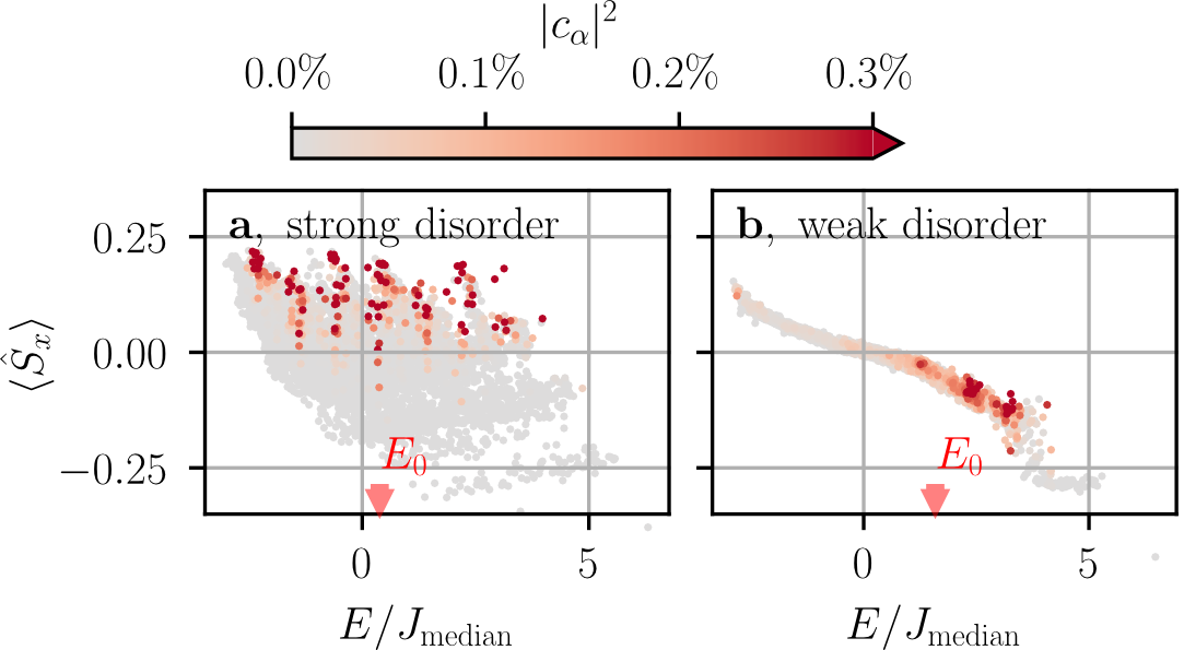
Figure 2: Eigenstate expectation values for the magnetization and eigenstate occupation numbers. Magnetization of each eigenstate $\alpha$ for a single disorder realization of 14 spins in a small negative locking field $\Omega=-0.3J_{\mathrm{median}}$ for strong a and weak disorder b as defined in Figure 1. The color code shows the overlap $|c_{\alpha}|^{2}$ of each eigenstate with the initial state. Additional data like the distributions $\rho(E)$ of the thermal ensembles and the density of states are provided in appendix F.

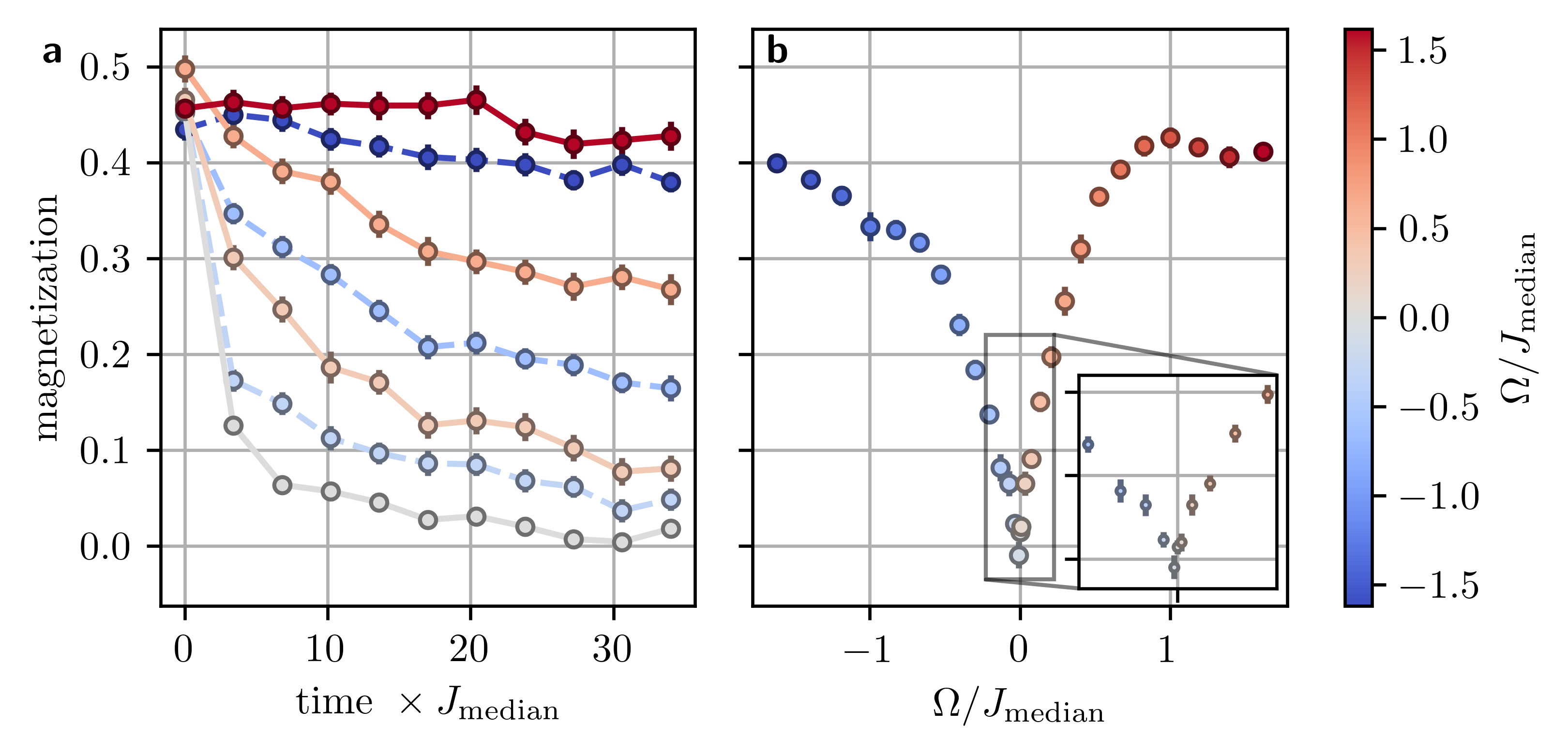
Figure 3: Relaxation dynamics of the magnetization and late time magnetization as function of the transverse field in a cloud of 3000 spins. a, Measured spin relaxation dynamcics for Van-der-Waals interactions for varying transverse field strengths ranging from $5.5\text{\,}\mathrm{MHz}$ (red) to $\Omega=$-5.5\text{\,}\mathrm{MHz}$$. b, Magnetization after $5\text{\,}\mathrm{\SIUnitSymbolMicro s}$ as a function of field strength $\Omega$ for Van-der-Waals interactions. The inset shows a zoom of the magnetization in vicinity of vanishing fields. The data was taken in a cloud of approximately 3000 spins with a median interaction strength of $J_{\mathrm{median}}=$3.4\text{\,}\mathrm{MHz}$$.

The observed absence of thermalization at strong disorder in numerical simulations of small systems of 14 spins is associated with a breakdown of the ETH. In order to illustrate this point, we analyze the eigenspectrum in Fig. 2. We find that at strong disorder (panel a), the eigenstate populations $|c_{\alpha}|^{2}$ (color encoded) are spread out over the entire spectrum, whereas, at weak disorder (panel b), eigenstates are populated mostly around $E_{0}$ (indicated by the red arrow). Also, the distribution of eigenstate expectation values $\mathcal{O}_{\alpha\alpha}$ for $\hat{\mathcal{O}}=\sum_{i}\hat{s}_{x}^{(i)}/N$ at any given energy is very broad in the case of strong disorder. In contrast, the magnetization expectation values are a smooth function of $E_{\alpha}$ in the case of weak disorder. We thus conclude that for small spin systems spectral localization of the initial state (ii) and ETH (iii) are violated for strong disorder.

The numerically observed breakdown of ETH can be understood within the simplified picture that spins can either be part of a strongly interacting pair or perfectly pinned by the external field (see Fig. 1 c). Within this picture two eigenstates can have similar energy while largely differing in magnetization because the energy penalty of flipping many spins can be compensated by changing the state of one strongly interacting pair, thus explaining the broad distribution observed in Fig. 2a. Conversely, two eigenstates with similar magnetization can be energetically far separated if they feature a strongly interacting pair in two different eigenstates leading to a large spectral spread of $|c_{\alpha}|^{2}$. This shows that the breakdown of ETH is rooted in the existence of strongly interacting pairs that effectively decouple from the rest of the system. Thus, the projectors onto the eigenstates of these pairs take the role of local integrals of motion, which in standard MBL models with random local fields are given by the individual spins [41, 42, 43]. We provide a more detailed discussion of the spectral properties in Appendix F.

We conclude from our numerical study that the non-negativity of the late time magnetization and its non-analytic dependence on $\Omega$ differ qualitatively from thermal ensemble predictions and are thus a clear sign of disorder-induced failure of thermalization. Many-body localization phenomena are known to be prone to finite size effects [19] which motivates us to probe the persistence of these features at significantly larger system sizes through a quantum simulation experiment.

IV Experimental signatures of breakdown of thermalization

In our experiment, we encode the spin degree of freedom in highly excited Rydberg states $\ket{\downarrow}=\ket{61S}$ and $\ket{\uparrow}=\ket{62S}$ leading to Van-der-Waals interactions as described by Eq. (2) with $\delta=$-0.7$$, $a=6$ and $C_{6}/(2\pi)=$1000\text{\,}\mathrm{GHz}\text{\,}{\mathrm{\SIUnitSymbolMicro m}}^{6}$$. By coupling the spin states with a microwave field $\Omega$, we can initialize the spins in the $x$-polarized initial state $\ket{\psi_{0}}=\ket{\rightarrow}^{\otimes N}$, implement the external field $\hat{H}_{\mathrm{ext}}$ and read out tomographically the final magnetization (see methods for details of the experimental protocol). We choose the density of the Rydberg cloud such that the median interaction strength $J_{\mathrm{median}}/(2\pi)=$6.8\text{\,}\mathrm{MHz}$$ is large compared to the decay rate of the Rydberg atoms of $\Gamma/(2\pi)=$0.06\text{\,}\mathrm{MHz}$$ (see methods for more details on the distribution of the Rydberg atoms). At this density, the blockade radius $r_{\mathrm{bl}}=$5.7\text{\,}\mathrm{\SIUnitSymbolMicro m}$$ is still small compared to the close-packing limit $r_{\mathrm{max}}=$14\text{\,}\mathrm{\SIUnitSymbolMicro m}$$, corresponding to the strong disorder regime (see Fig. 1 d).

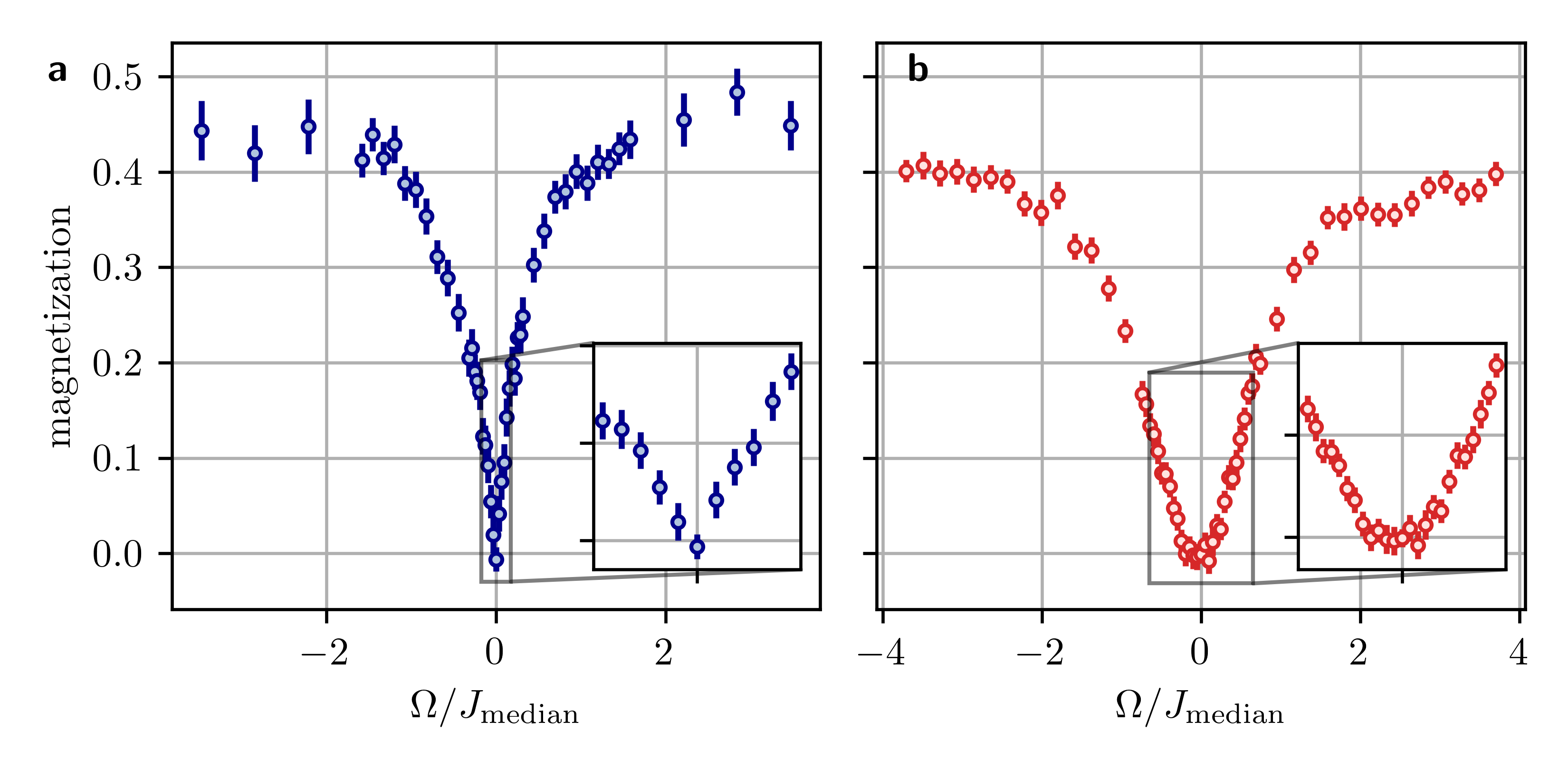
Figure 4: Late time magnetization for different strength of disorder for a spin system interacting with dipole-dipole interactions. a, At low density ($N=1150$, $J_{\mathrm{median}}=$1.4\text{\,}\mathrm{MHz}$$), corresponding to strong disorder ($r_{\mathrm{bl}}=0.3r_{\mathrm{max}}$), the late time magnetization exhibits the non-analyticity at zero field $\Omega$ expected for a non-thermal system. b, In the case of high density ($N=3900$, $J_{\mathrm{median}}=$2.7\text{\,}\mathrm{MHz}$$), respectively weak disorder ($r_{\mathrm{bl}}=0.5r_{\mathrm{max}}$), the late-time magnetization is a smooth function of the external field $\Omega$, indicating the system to be thermalized.

The dynamics for different field strengths are shown in Fig. 3 a. For $\Omega=0$ the system fully depolarizes after a few microseconds. For a weak field, the dynamics display the same rapid initial decay over $1\text{\,}\mathrm{\SIUnitSymbolMicro s}$ followed by slow saturation dynamics up to $10\text{\,}\mathrm{\SIUnitSymbolMicro s}$. The saturation value of the magnetization depends on the strength and the sign of the external field which is expected due to the spin locking mechanism explained above. Figure 3b shows the late-time value of the magnetization (taken after $10\text{\,}\mathrm{\SIUnitSymbolMicro s}$) as a function of the field strength. This curve features the same characteristics as the diagonal ensemble prediction obtained from exact diagonalization in the case of strong disorder (Fig. 1 d): In particular, we highlight the non-analytic feature at $\Omega=$0\text{\,}\mathrm{MHz}$$, which we had identified as inconsistent with thermal ensemble predictions. We thus observe that a system of 3000 spins fails to reach a thermal state on time scales exceeding the typical relaxation time of the system.

V Restoring thermalization in long-range interacting spin systems

Exploiting the full versatility of the Rydberg platform, we can tune the range of interaction by implementing a dipolar interacting spin system using the Rydberg states $\ket{\downarrow}=\ket{48S}$ and $\ket{\uparrow}=\ket{48P}$. For the resulting Hamiltonian with $\delta=0$, $C_{3}/(2\pi)=$1.15\text{\,}\mathrm{GHz}\text{\,}{\mathrm{\SIUnitSymbolMicro m}}^{3}$$ and a spatial anisotropy $J_{ij}(\theta)=(1-3\cos(\theta)^{2})/2$, the interaction range $a=3$ equals the dimension $d=3$ of the system. Resonance counting arguments suggest that for $a>d$ the system should no longer be localized [17], rendering the critical case $a=d$ a particularly interesting one, even more so as numerical simulations strongly suffer from finite size effects in this case (see appendix G). Our experiments enable us to study this case for system sizes increased more than 100-fold compared to what is accessible numerically.

Fig. 4a shows the late-time dynamics taken after $10\text{\,}\mathrm{\SIUnitSymbolMicro s}$ for dipolar interaction in the strongly disordered regime of $r_{\mathrm{bl}}=0.3r_{\mathrm{max}}$ (time resolved data is provided in appendix B). Interestingly, this curve strongly resembles the case of the Van-der-Waals spin system: At large fields, $\Omega>$2.5\text{\,}\mathrm{MHz}$$, compared to $J_{\mathrm{median}}\approx$1.4\text{\,}\mathrm{MHz}$$, the magnetization is locked to the initial value. The asymmetry is strongly reduced because the sign of the interaction strength is angular dependent and no longer purely repulsive. Most importantly, the sharp cusp feature has remained unchanged, which suggests the absence of thermalization also in the case of a strongly disordered dipolar system.

Finally, to show that thermalizing behavior is established at weaker disorder, we have saturated the Rydberg excitations in the cloud in a strongly blockaded regime where $r_{\mathrm{bl}}=0.5r_{\mathrm{max}}$. In this case, as shown in see Fig. 4 b, the cusp feature disappears and a smooth dependence on the external field strength is recovered, qualitatively agreeing with thermal ensemble predictions.

VI Discussion and Outlook

We have observed non-thermalizing dynamics of powerlaw interacting spins with positional disorder by studying late-time magnetization after a quantum quench. The observed magnetization equilibrates rapidly under the unitary dynamics, and thermal ensemble predictions differ qualitatively from the observed late-time values (Appendix J). Recent theoretical works claim that systems with power-law interactions or with dimensions $D>1$ thermalize due to rare ergodic regions that seed thermalizing avalanches [10, 13, 14, 15, 11] in the limit of infinite system sizes and evolution times. Yet, our observations demonstrate the absence of thermalization as expected for a system that is in a MBL phase. Thus, adopting the terminology of [11], we interpret our observation as an MBL regime, i.e. localization effects occurring at finite times and system sizes. We also note that the proliferation of thermalization avalanches should depend on the coordination number of the interaction graph (rather than the spatial dimension), which becomes small in the strongly disordered limit of our model [44, 45]. This would be consistent with the reestablishment of thermalization for more strongly correlated coupling constant corresponding to an increased coordination number. The characteristic features of our system, power-law interactions and static positional disorder, are naturally realized by a wide range of quantum simulation platforms beyond Rydberg atoms, including nuclear spins [46], color centers in diamond [47], polar molecules [48] and magnetic atoms [49, 50]. Our work thus paves a way to study quantum thermalization for a largely unexplored type of disordered systems in a scalable fashion.

VII Acknowledgements

We acknowledge Shannon Whitlock, Renato Ferracini Alves, and Asier Piñeiro Orioli for contributing to the preliminary work for this study. We thank Dmitry A. Abanin and M. Rigol for helpful discussions. This work is part of and supported by the Deutsche Forschungsgemeinschaft (DFG, German Research Foundation) under Germany’s Excellence Strategy EXC2181/1-390900948 (the Heidelberg STRUCTURES Excellence Cluster), within the Collaborative Research Centre “SFB 1225 (ISOQUANT),” the DFG Priority Program “GiRyd 1929,” the European Union H2020 projects FET Proactive project RySQ (Grant No. 640378), and FET flagship project PASQuanS (Grant No. 817482), and the Heidelberg Center for Quantum Dynamics. T. F. acknowledges funding by a graduate scholarship of the Heidelberg University (LGFG). This work is supported by Deutsche Forschungsgesellschaft (DFG, German Research Foundation) under Germany’s Excellence Strategy EXC2181/1-390900948 (the Heidelberg STRUCTURES Excellence Cluster). The authors acknowledge support by the state of Baden-Württemberg through bwHPC and the German Research Foundation (DFG) through Grant No. INST 40/575-1 FUGG (JUSTUS 2 cluster).

Methods

Here we provide further details on the numeric simulations and both the experimental protocol and the spatial configuration of the Rydberg cloud.

Details on numerical simulations. To diagonalize Hamiltonian (2), we take into account the parity symmetry with respect to a global spin-flip $P_{s}=\prod_{i}^{N}\hat{\sigma}_{x}^{(i)}$ which reduces the dimension of the Hilbert space by a factor of two and ensures that the thermal ensemble calculations only take eigenstates into account states that have the same (positive) spin parity as the initial state $\ket{\psi_{0}}$.

To obtain the microcanonical expectation value, an appropriate energy window $\Delta_{E}$ needs to be chosen. In the thermodynamic limit, the size of this window should vanish $\Delta_{E}\rightarrow 0^{+}$. However, for finite-size systems, the energy window needs to be finite to ensure that a sufficient number of eigenstates contributes to the microcanonical ensemble. In Fig. 8 in appendix D we compare the microcanonical expectation values for energy windows ranging from $10^{-6}J_{\mathrm{median}}$ to $10^{1}J_{\mathrm{median}}$ and find that the microcanonical ensemble simulation is independent of the energy window $\Delta_{E}$ signifying that the finite window size does not change the microcanonical expectation values.

Details on experimental implementation. We start the experiment by trapping $10^{6}$ Rubidium-87 in a cigar shaped dipole trap with a diameter of $300\text{\,}\mathrm{\SIUnitSymbolMicro m}$ (long axis) and $70\text{\,}\mathrm{\SIUnitSymbolMicro m}$(short axis) at a temperature of $10\text{\,}\mathrm{\SIUnitSymbolMicro K}$. We consider this gas to be frozen since the atoms move only a distance of $d_{\text{kin}}=t_{\text{exp}}\sqrt{\frac{3kT}{m}}=$0.5\text{\,}\mathrm{\SIUnitSymbolMicro m}$$ during an experimental cycle of $t_{\text{exp}}=$10\text{\,}\mathrm{\SIUnitSymbolMicro s}$$ which is small compared to the Rydberg blockade radius of $r_{\mathrm{bl}}\approx$5\text{\,}\mathrm{\SIUnitSymbolMicro m}$$. After optically pumping the atoms into the state $\ket{5S(F=2,m_{F}=2)}$, we optically excite the atoms to the spin state $\ket{\downarrow}$ via a two-photon off-resonant excitation process (single-photon detuning of $98\text{\,}\mathrm{MHz}$ and two-photon Rabi frequency of $1\text{\,}\mathrm{MHz}$). A global microwave $\pi/2$-pulse prepares the fully polarized initial state $\ket{\psi_{0}}=\ket{\rightarrow_{x}}^{\otimes N}$. In the case of Van-der-Waals interactions, the state $\ket{61}S$ is coupled resonantly to $\ket{62}S$ via a two-photon transition at a microwave frequency of $16.546\text{\,}\mathrm{GHz}$ which can be directly generated with a Keysight M8190A arbitrary waveform generator (AWG). For the dipolar interacting spin system, we couple the $\ket{48S}$ state resonantly with a single-photon transition at $35\text{\,}\mathrm{GHz}$. This frequency is generated by mixing a $5\text{\,}\mathrm{GHz}$ signal of the Keysight M8190A AWG with an Anritsu MG3697C signal generator. The same microwave setup is used to realize the spin locking field where a phase shift of 90 degrees needs to be added such that the field aligns with the spins. This allows us to implement the transverse field term, Eq. (3), with field strengths up to $\Omega/(2\pi)=$10\text{\,}\mathrm{MHz}$$. After a time evolution $t$, the $x$-magnetization is rotated tomographically onto the $z$-axis by applying a second $\pi/2$-pulse with various phases. Finally, the magnetization is obtained from a measurement of the population of one of the two spin states via field ionization, and the other spin state is optically deexcited to the ground state. A visual representation of the measurement protocol can be found in appendix A, and a more detailed explanation of the determination of the magnetization was reported in a previous publication [7].

Details on the Rydberg distribution. In this work, we can tune the disorder with the Rydberg blockade effect, which imposes a minimal distance $r_{\mathrm{bl}}$ between the spins. At small blockade radius, the spins are distributed randomly in the cloud, while a large radius introduces strong correlation between the atom positions and hence the coupling strength. To quantify the disorder strength, we compare the blockade radius to the distance ${r_{\mathrm{max}}}=2[3\eta_{\mathrm{cp}}/(4\pi\rho)]^{1/3}$ which corresponds to the distance between the spins in a close-packed arrangement at same density $\rho$ and packing fraction $\eta_{\mathrm{cp}}=\pi/\sqrt{18}\approx 0.74$.

In our experiment, we tune the spatial distribution of the Rydberg atoms by varying the volume of the ground state atoms with a short time-of-flight period after turning off the dipole trap and before exciting to the Rydberg states. Further, we can alter the Rydberg fraction by modifying the excitation time $t_{\mathrm{exc}}$. We measure the resulting Rydberg density through depletion imaging [51] where we deduce the Rydberg distribution from the ground state atoms that are missing after Rydberg excitation. The measured parameters of the Rydberg distribution are presented in detail in Table 1 in appendix A.

To estimate the Rydberg blockade radius, we model the excitation dynamics by the simplified description introduced in [7] which assumes a hard-sphere model for the Rydberg blockade effect. This model sets an upper limit on the blockade radius $r_{\mathrm{bl}}=\sqrt[6]{\frac{C_{6}}{\Gamma_{\mathrm{eff}}}}$ by estimating the effective linewidth of the laser, based on the duration of the excitation pulse and power broadening. The latter is calculated self-consistently, taking into account the enhancement factor induced by collective Rabi oscillations within a superatom [52, 53].

This established model of the Rydberg cloud can be benchmarked using the experimentally measured time evolution without a locking field, which is known to be well described by semiclassical Discrete Truncated Wigner Approximation (DTWA) [7] (see Fig. 7 in appendix C). This simulation is highly sensitive to the exact value of the blockade radius, and we can deduce that the hard-sphere model slightly overestimates the Rydberg blockade effect in the case of Van-der-Waals interactions where a fitted value of $r_{\mathrm{bl}}=$5.7\text{\,}\mathrm{\SIUnitSymbolMicro m}$=0.4r_{\mathrm{max}}$ describes the experiment perfectly. For the more long-range dipolar interactions, the blockade radius of $r_{\mathrm{bl}}=$6.5\text{\,}\mathrm{\SIUnitSymbolMicro m}$=0.5r_{\mathrm{max}}$ is already a reasonable estimate leading to a good agreement between the experiment and DTWA simulation.

From the excitation model, we can also compute the median of the nearest neighbor interaction strength $J_{\mathrm{median}}$ which ranges from $0.78\text{\,}\mathrm{MHz}$ to $3.4\text{\,}\mathrm{MHz}$ depending on the experimental setting (see table 1). The resulting time evolution can be considered unitary for up to $10\mu s$ which is an order of magnitude larger than the timescale of the experiment $J_{\mathrm{median}}^{-1}$.

Appendix A Illustration of the experimental protocol and parameters

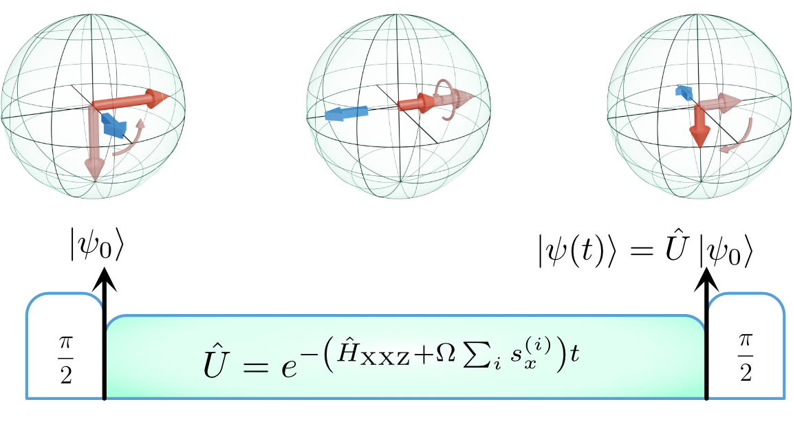
Figure 5: Experimental protocol: An initial $\pi/2$-pulse aligns the spins in $x$-direction. After unitary dynamics under the interaction Hamiltonian and the locking field, a second $\pi/2$-pulse with varying phases reads out the magnetization in the $xy$-plane. For each pulse, the Bloch spheres illustrate the spin state of the initial state (light red arrow), the final state (red arrow), and the direction of the external field (blue arrow).

	Van-der-Waals interactions (Figure 3 a and b)	Dipolar interactions (low density) (Figure 4 a)	Dipolar interactions (high density) (Figure 4 b)
$t_{\mathrm{exc}}$	$5\text{\,}\mathrm{\SIUnitSymbolMicro s}$	$1\text{\,}\mathrm{\SIUnitSymbolMicro s}$	$10\text{\,}\mathrm{\SIUnitSymbolMicro s}$
Rydberg volume	$$69\text{\,}\mathrm{\SIUnitSymbolMicro m}$\times$43\text{\,}\mathrm{\SIUnitSymbolMicro m}$\times$37\text{\,}\mathrm{\SIUnitSymbolMicro m}$$	$$59\text{\,}\mathrm{\SIUnitSymbolMicro m}$\times$44\text{\,}\mathrm{\SIUnitSymbolMicro m}$\times$36\text{\,}\mathrm{\SIUnitSymbolMicro m}$$	$$59\text{\,}\mathrm{\SIUnitSymbolMicro m}$\times$34\text{\,}\mathrm{\SIUnitSymbolMicro m}$\times$30\text{\,}\mathrm{\SIUnitSymbolMicro m}$$
$N_{\text{Ryd}}$	2900	1150	3900
$r_{\mathrm{bl}}$	$$5.7\text{\,}\mathrm{\SIUnitSymbolMicro m}$=0.4r_{\text{max}}$	$$5.3\text{\,}\mathrm{\SIUnitSymbolMicro m}$=0.29r_{\text{max}}$	$$6.5\text{\,}\mathrm{\SIUnitSymbolMicro m}$=0.5r_{\text{max}}$
$J_{\text{median}}$	$3.4\text{\,}\mathrm{M}\mathrm{H}\mathrm{z}$	$0.78\text{\,}\mathrm{M}\mathrm{H}\mathrm{z}$	$1.7\text{\,}\mathrm{M}\mathrm{H}\mathrm{z}$

Table 1: Experimental parameters. $t_{\mathrm{exc}}$ specifies the duration of the optical excitation to the Rydberg state, the Rydberg volume is specified by the radii ($1/e^{2}$) of the Rydberg cloud, $N_{\text{Ryd}}$ denotes the derived Rydberg number, $r_{\mathrm{bl}}$ the blockade radius and $J_{\text{median}}$ the obtained median nearest-neighbor interaction.

Appendix B Time evolution of the dipolar interacting spin system

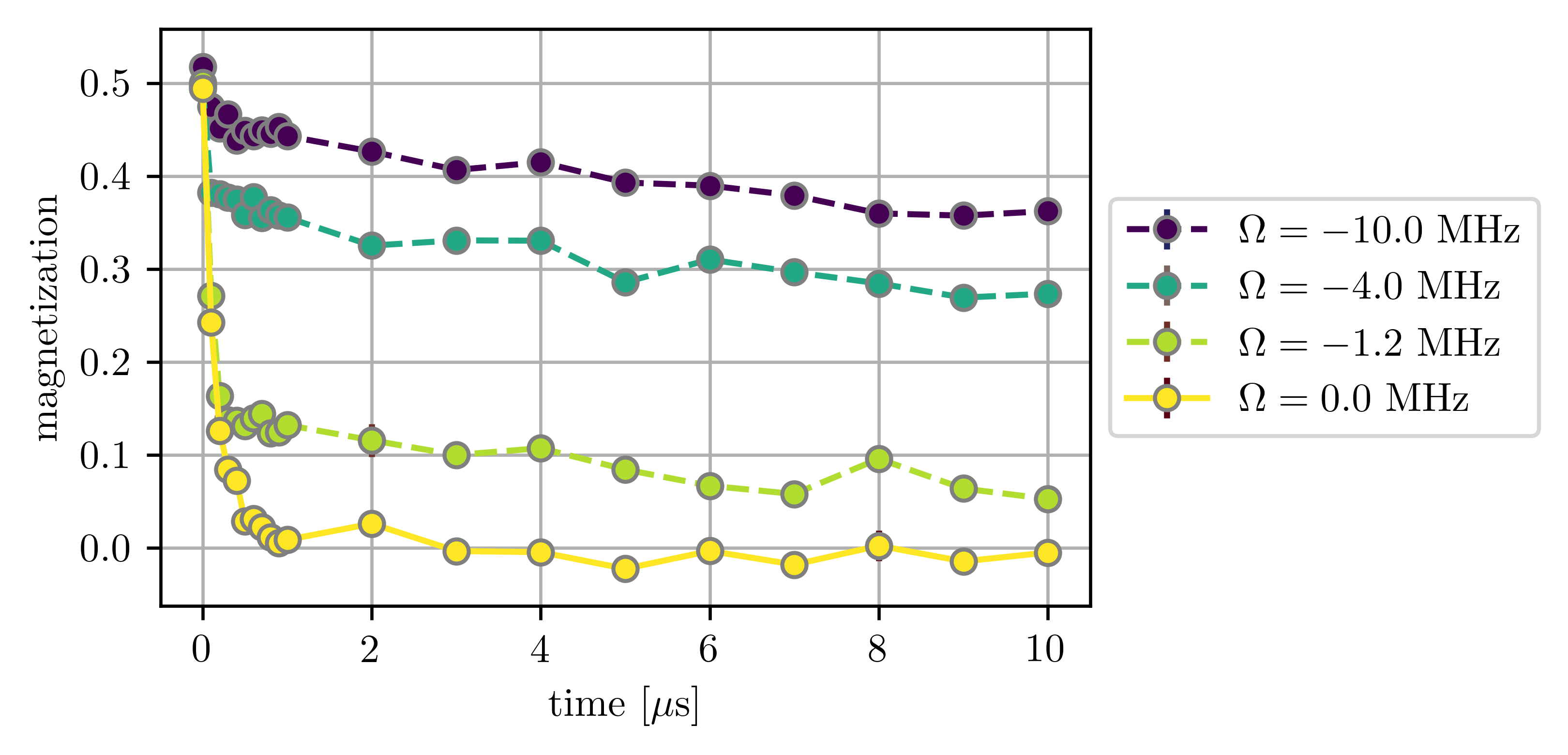
Figure 6: Time evolution of the dipolar interacting spin system. The experimental parameters for the time traces are identical to the quantum simulation shown in Fig. 4 b in the main text.

Analogously to Fig. 3 a in the main text, we also measured the time evolution of the magnetization for the dipolar interacting Rydberg spin system in the case of strong disorder for various external fields $\Omega$. The resulting dynamics are shown in Fig. 6. Similar to the case of Van-der-Waals interactions shown in Fig. 3 a in the main text, the magnetization relaxes within a microsecond to zero in the case of zero applied field ($\Omega=0$). With applied field, the dynamics show a rapid decay within the first microsecond, followed by a much slower relaxation until the final magnetization at $10\text{\,}\mathrm{\SIUnitSymbolMicro s}$ is reached. This late-time magnetization is plotted as a function of the external field in Fig. 4 in the main text.

Appendix C Semiclassical simulations of the Ramsey decay

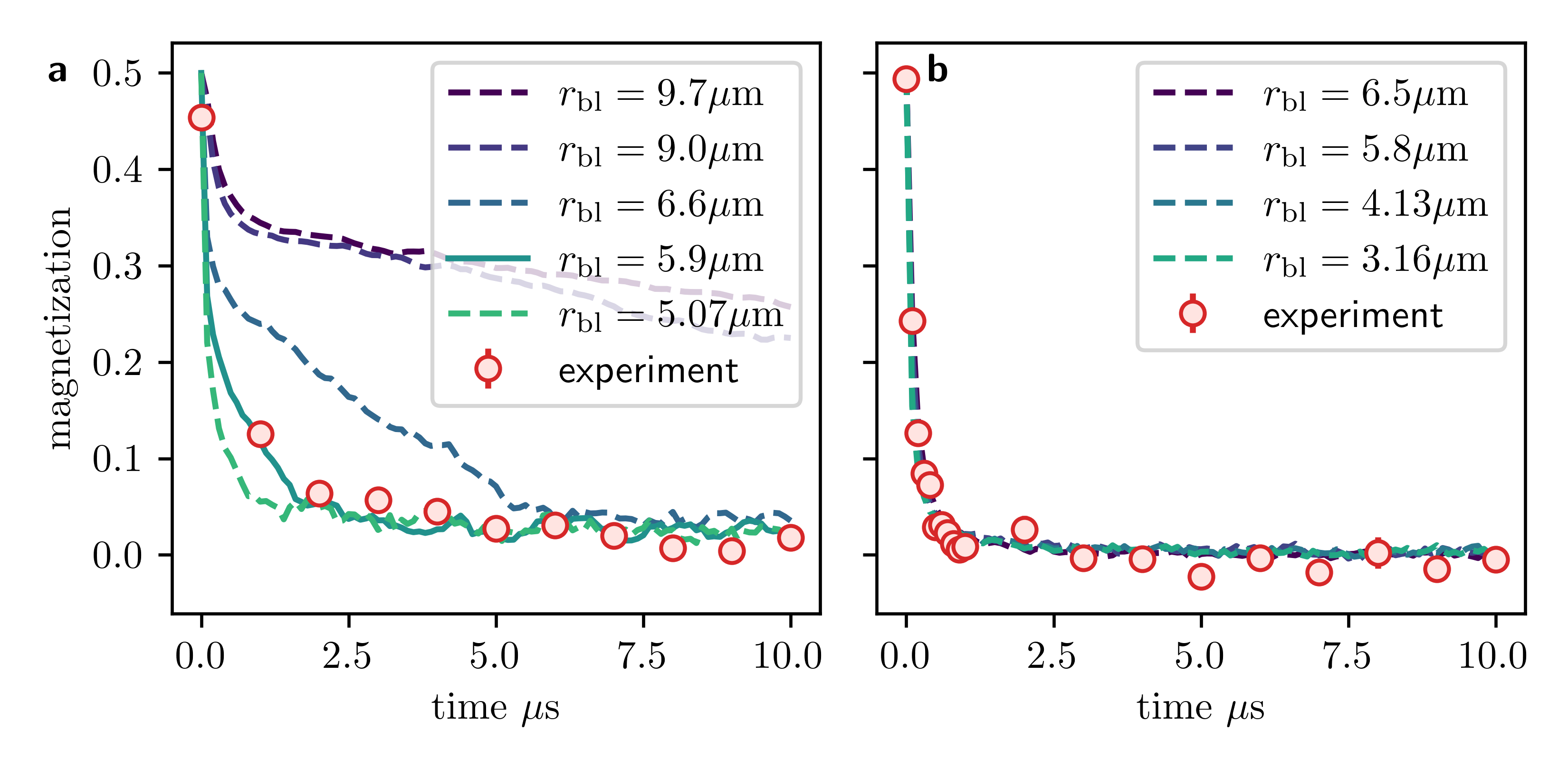
Figure 7: Semiclassical simulations using Discrete Truncated Wigner Approximation (DTWA) in the case of Van-der-Waals interactions (a) and dipolar interactions (b). The simulations are performed for realistic distributions of the Rydberg spins with the same density as the experiment (red dots), but for varying blockade radii. The maximal blockade radius corresponds to a linewidth of the Rydberg excitation determined by Fourier limit and power broadening. The simulation best fitting the experimental data is plotted as a solid line.

In previous work [54, 7], we could show that the semiclassical Discrete Truncated Wigner Approximation (DTWA) is well suited to describe the relaxation of the magnetization under the interaction Hamiltonian (2) defined in the main text. The main principle of DTWA is to sample classical time evolutions over different initial states such that the quantum uncertainty of the initial state is respected [55]. In Fig. 7, we compare the time evolution obtained from DTWA simulations for various blockade radii (solid lines) to the experimental data (red dots) in the case of Van-der-Waals (panel a) and dipolar interactions (panel b). It turns out that in the case of Van-der-Waals interactions, the resulting dynamics depend sensitively on the blockade radius, which allows estimating the correct blockade radius to be $5.9\text{\,}\mathrm{\SIUnitSymbolMicro m}$. This radius is small compared to the blockade radius of $7.8\text{\,}\mathrm{\SIUnitSymbolMicro m}$ estimated from power broadening and the Fourier limit determined from the length of the excitation pulse. This discrepancy in expected and simulated blockade radius might be explained by a finite linewidth of the excitation lasers, a small detuning [56] or from underestimated Rydberg-Rydberg interactions. In the case of dipolar interactions, the DTWA dynamics are less sensitive to the size of the blockade radius. The reason might be the longer-range interactions which cause the dynamics to be less dominated by the nearest neighbors. As a result, the dynamics for a Rydberg distribution with a blockade radius estimated from the Fourier limit agrees already well with the experimental observation.

Appendix D Sensitivity of the microcanonical ensemble on the energy window

To calculate the magnetization expectation value of the microcanonical ensemble, the average over all eigenstate expectation values within an energy window $\Delta_{E}$ is calculated. In the thermodynamic limit, it is possible to calculate the limit $\Delta_{E}\rightarrow 0$, but for a finite simulation, the energy window has to be chosen small but finite. To ensure that the choice of the energy window does not influence the magnetization expectation value of the microcanonical ensemble, we compare in Fig. 8 a the prediction of microcanonical ensembles for a large range of energy windows between $10^{-4}J_{\mathrm{median}}$ and $10^{1}J_{\mathrm{median}}$. Indeed, we find that the simulations agree if the energy window is small enough, i.e. $\Delta_{E}/J_{\rm{median}}<10^{-3}$. In particular, all curves are smooth and feature a negative magnetization at small negative fields. The existence of this large region of energy windows is a strong hint that the microcanonical expectation value is no longer dependent on details of the finite size system, indicating that the simulation is already converged for 14 spins. Importantly, any microcanonical ensemble prediction differs qualitatively from the diagonal ensemble (red dashed line in Fig. 8 a) for any choice of $\Delta_{E}$.

Fig. 8 b shows how many eigenstates are populated within a given energy window $\Delta_{E}$. This quantity is important to ensure that the window size is varied in a meaningful way, i.e. that a different number of eigenstates are populated for different window sizes. For the smallest window, on average less than a single eigenstate is populated  which leads to large fluctuations of the magnetization. Contrary, for a large energy window of $10^{1}J_{\mathrm{median}}$, almost all eigenstates are populated by the microcanonical ensemble. Within the region where $\Delta_{E}/J_{\rm{median}}<10^{-3}$ and the microcanonical ensemble is converged, the number of populated eigenstates varies from 1 to 300 which highlights the insensitivity of the microcanonical ensemble with respect to the width of the energy window.

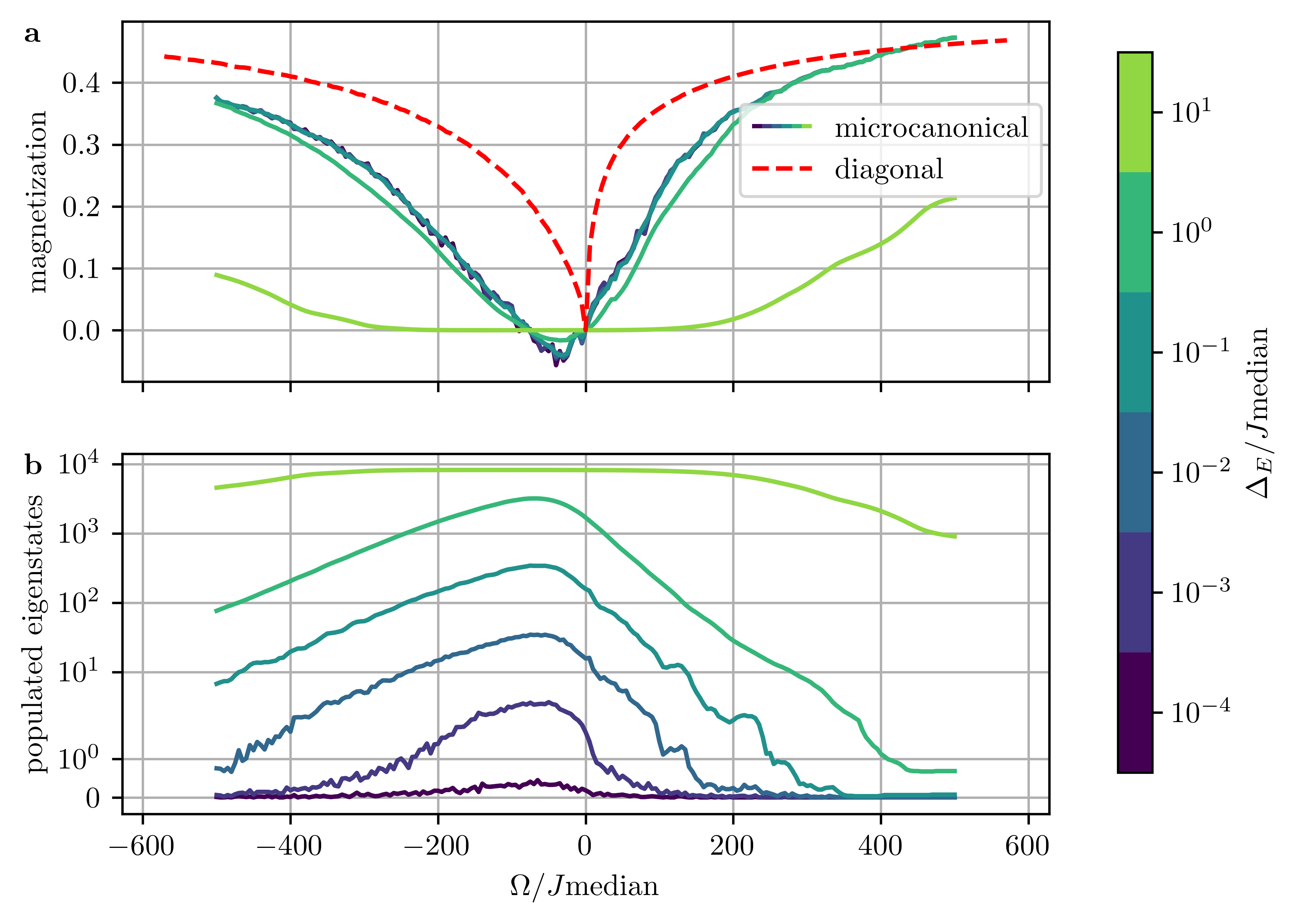
Figure 8: Microcanonical ensemble for different widths of the energy window $\Delta_{E}$ ranging from $10^{-6}J_{\mathrm{median}}$ to $10{1}J_{\mathrm{median}}$. The simulations are performed for the same system parameters as in Figure 1 of the main text (Heisenberg XXZ interactions with anisotropy $\delta=-0.7$, power law interactions $J_{ij}=\frac{C_{6}}{r^{6}}$, 100 disorder averages, 14 spins randomly distributed in a sphere with a minimal distance between the spins of $r_{\text{bl}}=0.4r_{\max}$). a, Magnetization as a function of $\Omega/J_{\mathrm{median}}$ for the microcanonical ensembles for different energy windows $\Delta_{E}$ (solid lines) and the diagonal ensemble (dashed red line). b, Number of populated eigenstates as a function of $\Omega/J_{\mathrm{median}}$ for different energy windows $\Delta_{E}$.

Appendix E Ensemble equivalence

In this work, we exemplary compute the microcanonical expectation values to show the behavior of a thermal system. It should be noted that one could as well choose the canonical ensemble $\langle\widehat{\mathcal{O}}\rangle_{\mathrm{c}}=Z^{-1}\sum_{\alpha}\mathcal{O}_{\alpha\alpha}e^{-\beta E_{\alpha}}$ (with inverse temperature $\beta$ satisfying $E_{0}=\langle\hat{H}\rangle_{\mathrm{c}}$ and partition function $Z$) as thermal ensembles become equivalent in the limit of large system sizes for short-range interacting systems [9]. Indeed, we find good agreement between the microcanonical ensemble and the canonical ensemble expectation value in the case of both strong and weak disorder (see Fig. 9). This agreement shows that thermal ensemble equivalence already holds at this moderate system size of 14 spins.

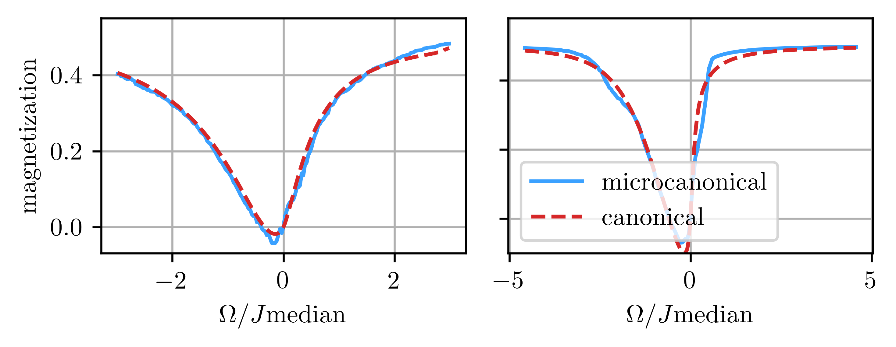
Figure 9: Comparison of the microcanonical (solid blue line) and the canonical ensemble (dashed red line) in the case of strong (panel a) and weak disoroder (panel b). For each thermal ensemble, the magnetization is plotted as a function of the external field $\Omega$

Appendix F Spectral properties for varying disorder strength

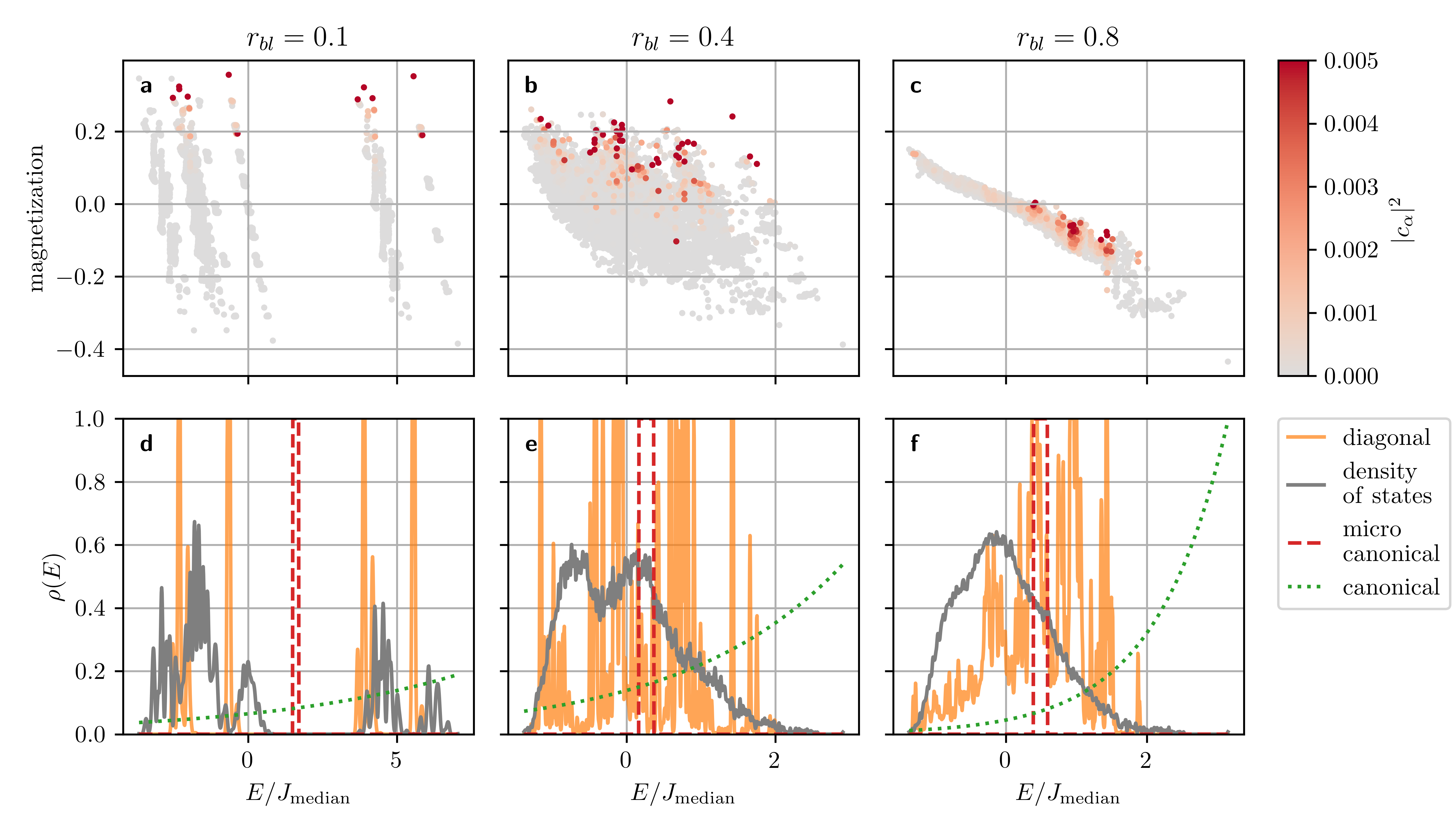
Figure 10: Same as Fig. 2 with three different blockade radii $r_{\mathrm{bl}}=0.1a_{0}$ (left column), $r_{\mathrm{bl}}=0.4a_{0}$ (central column), and $r_{\mathrm{bl}}=0.8a_{0}$ (right column). Top row (a - c: Eigenstate expectation value of the magnetization for a single disorder realization at $\Omega=-0.2J_{\mathrm{median}}$ for all eigenstates as a function of eigenenergy. The color encodes the eigenstate occupation $|\innerproduct{\psi_{0}}{\phi_{\alpha}}|^{2}$. Bottom row (d - f): Energy distributions $\rho(E)$ of the diagonal ensemble (solid orange line), microcanonical ensemble (dashed red line), and canonical ensemble (dotted green line) for the same disorder realization and field as in the top row. The solid gray line shows the density of states. The diagonal ensemble and density of states are obtained after a Gaussian kernel density estimation with bandwidth $0.01J_{\mathrm{median}}$, the energy gap of the microcanonical ensemble is $\Delta_{E}=0.1J_{\mathrm{median}}$.

Figure 10 gives additional details of the simulations shown in Fig. 1 and 2 of the main text. The middle and right columns represent the same simulation as in the main text for the strong and weak disordered systems, respectively.

The left column shows an even more strongly disordered case (smaller blockade radius), where all ensembles mutually disagree. For this very strong disorder, a sawtooth profile is visible where the magnetization in some regions of the spectrum depends linearly on energy (Fig. 10 a). As a consequence of extremely strong interacting pairs, the spectrum is energetically split into far apart blocks. In between, the density of states is zero (Fig. 10 d), which might be a sign of finite-size effects and indicate that the simulation is not yet converged to the thermodynamic limit. To explain how the sawtooth profile of the eigenstate expectation values emerges from disorder, we can consider a simplified scenario of a single strongly interacting pair where $J_{ij}^{\mathrm{strong}}\gg\Omega$ surrounded by $N$ weakly interacting spins where $\Omega\gg J_{ij}^{\mathrm{weak}}$ (see Fig. 1 a and c). To find approximate eigenstates for this system, we may first diagonalize the strongly interacting pair giving rise to two occupied eigenstates separated in energy by $J_{ij}^{\mathrm{strong}}$. The remaining spins can be approximately assumed to be non-interacting leading to $2^{N}$ configurations with energies $-\frac{N\Omega}{2},-\frac{(N-1)\Omega}{2},\dots,\frac{(N-1)\Omega}{2},\frac{N\Omega}{2}$. As a result, the spectrum is divided into two regions, each associated with one of the eigenstates of the strongly interacting pair; Within each region, magnetization is determined by the weakly interacting spins and depends linearly on energy with a slope $\frac{1}{N\Omega}$. In the case where $J_{ij}^{\mathrm{strong}}\approx N\Omega$, this scenario yields two states depicted by Fig. 1c of the main text that features similar eigenenergy but vastly different magnetization. We expect eigenstates where the weakly interacting spins are strongly polarized to share a significant wavefunction overlap with the fully magnetized initial state. However, these states may have completely different eigenenergies due to the internal state of the strongly interacting spins.

The central column shows a slightly less disordered system ("strong disorder" in the main text). Here, the microcanonical and canonical ensemble agree, but they differ from the diagonal one (Fig. 10 e). Like the strongly disordered case depicted in the left column of Fig. 10, strongly interacting pairs induce large variations of the eigenstate expectation values. However, due to the non-negligible blockade effect, the existence of extremely strong interacting pairs is prohibited. Therefore, the eigenspectrum is not split into clearly distinguishable blocks (Fig. 10 e), and as a consequence, the density of states becomes a smooth function without gaps. This smoothness might be indicative of a reasonable convergence of the simulation. Additional disorder realizations for this case are shown in Fig. 11. Qualitatively, they show very similar behavior, including a large variation of eigenstate expectation values and an extended spread of eigenstate occupation numbers.

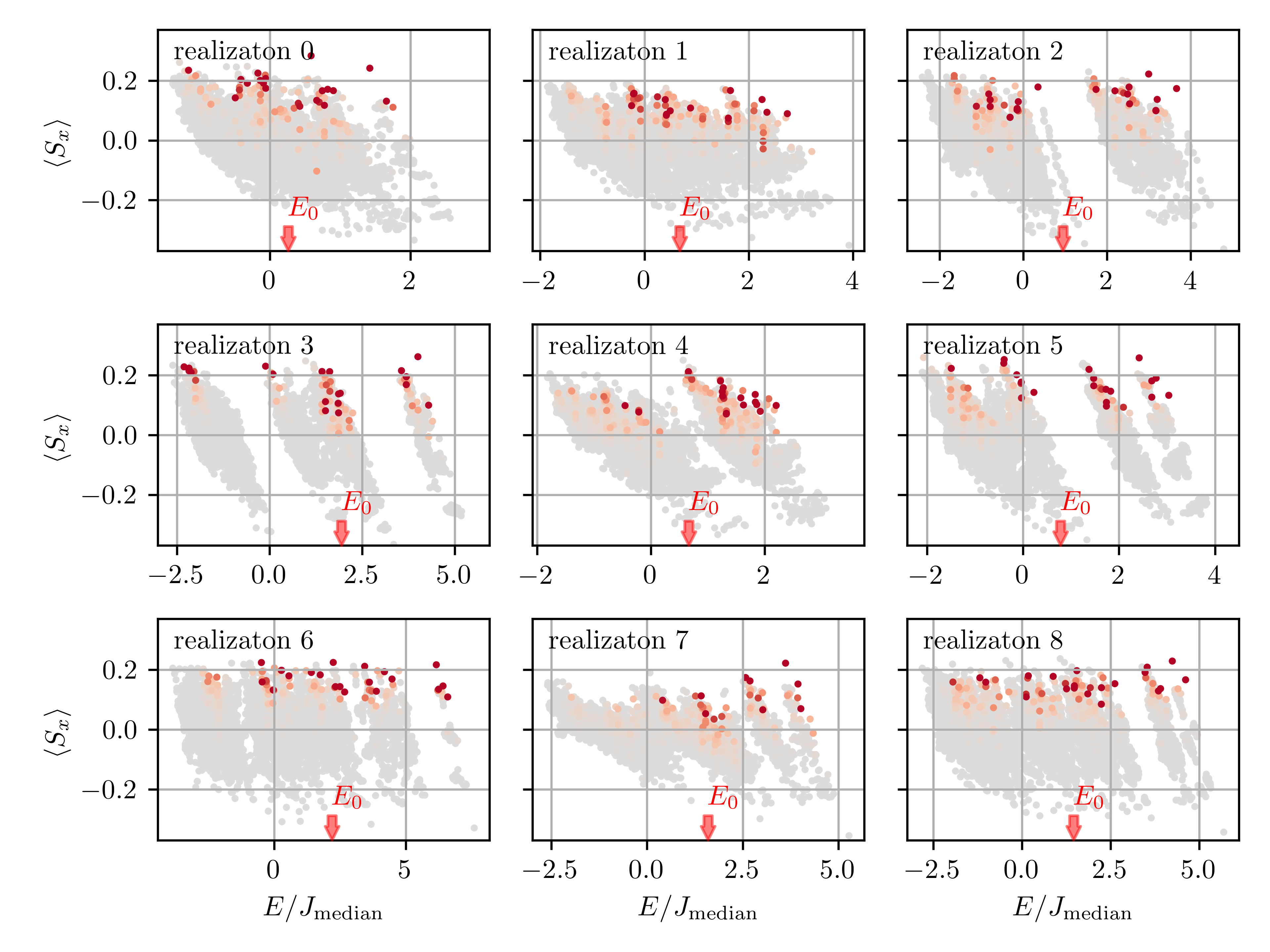
Figure 11: Similar to Fig. 10 b, Eigenstate expectation values of the magnetization for 9 different disorder realizations at $\Omega=-0.2J_{\mathrm{median}}$ and $r_{\mathrm{bl}}=0.4r_{\mathrm{max}}$ for all eigenstates as a function of eigenenergy. The color encodes the eigenstate occupation $|c_{\alpha}|^{2}=|\innerproduct{\psi_{0}}{\phi_{\alpha}}|^{2}$.

For weak disorder (right column in Fig. 10), all ensemble predictions agree, which indicates thermalization (Fig. 1 e). Quantum thermalization is confirmed by the eigenspectrum, which shows a smooth dependency of the eigenstate magnetization as a function of eigenenergy (Fig. 10 c) following ETH. Also, the eigenstate occupation (orange line in Fig. 10 f) is clearly peaked at the energy of the initial state as expected in a thermalizing system. However, this peak is still relatively broad compared to the energy window of the microcanonical ensemble (dashed red line in Fig. 10 i). This broadening of the eigenstate occupation number is a well-known finite size effect that is also present in other numerical studies [36].

Appendix G Numerical simulations for dipolar interactions

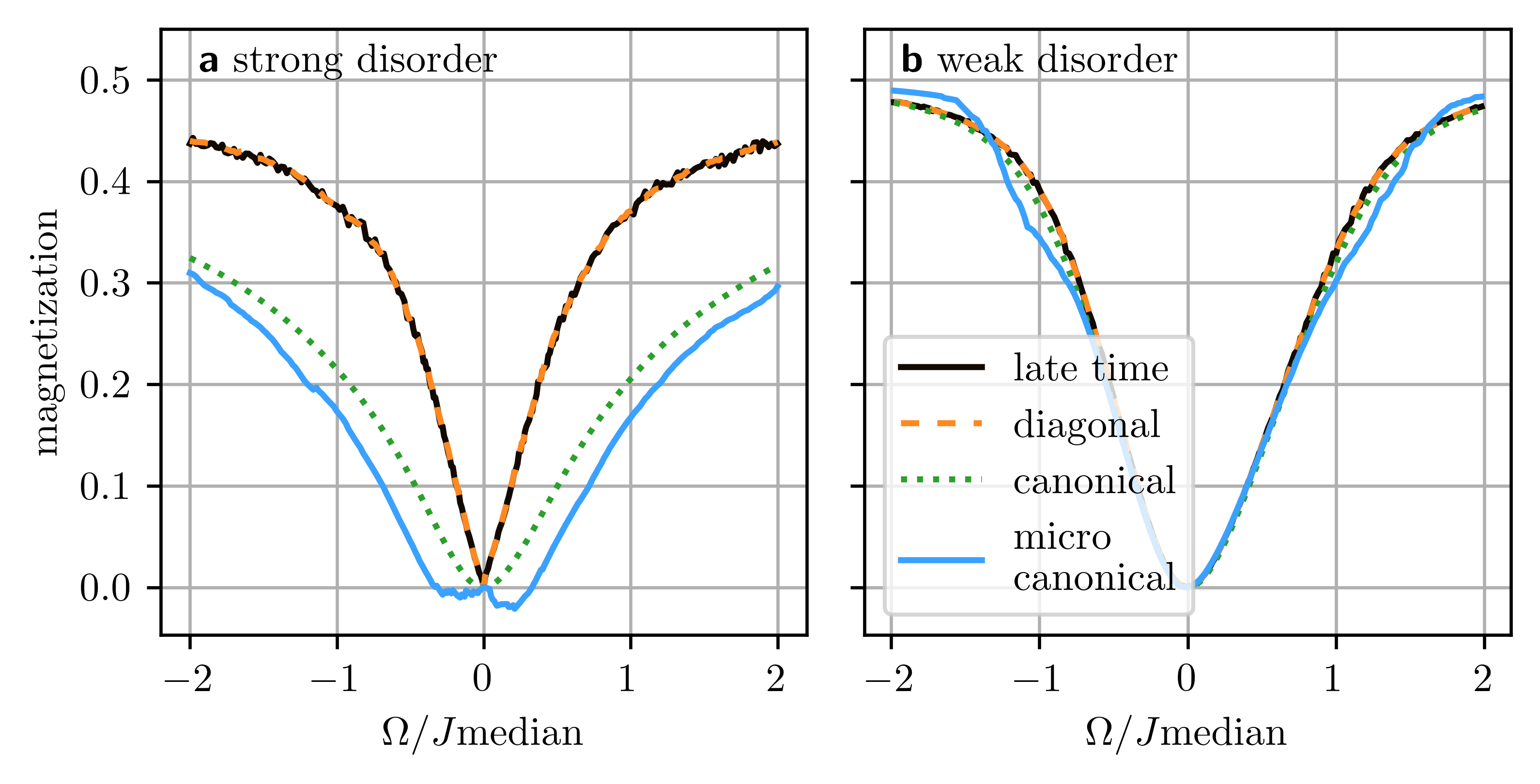
Figure 12: Similar to Fig. 1 d and e from the main text, but for dipolar interactions. The simulations are also obtained from 100 disorder averages by exact diagonalization of 14 spins, but the blockade radii are chosen differently ($r_{\mathrm{bl}}=0.01r_{\mathrm{max}}$ for strong disorder and $r_{\mathrm{bl}}=0.4r_{\mathrm{max}}$ weak disorder) to compensate for the more long-range interactions.

The simulations in the main text shown in Fig. 1 and 2 are performed in a Van-der-Waals interacting system with purely repulsive interactions and a power-law $a=6$. Changing the system to dipolar interaction modifies these two characteristics: The sign of the interactions becomes dependent on the angle $\theta$ between the quantization axis and the interatomic axis proportional to $1-3\cos(\theta)^{2}$ and the interactions are more long-range with $a=3$. This section will investigate how these changes alter the system dynamics and the steady-state properties.

Fig. 12 compares the late-time magnetization (dashed black line), the diagonal ensemble (solid orange line), the microcanonical ensemble expectation value (solid blue line) and the canonical ensemble (dotted green line) in the case of strong (panel a) and weak disorder (b). As in the case of Van-der-Waals interactions, the late-time magnetization agrees almost perfectly with the diagonal ensemble for both strong and weak disorders. This agreement shows that the system has equilibrated to a steady-state. Also, we can observe that the thermal ensembles (canonical and microcanonical) agree with the steady-state only in the case of weak disorder. For strong disorder, the thermal ensembles predict a magnetization being consistently lower than the steady-state value. This disagreement indicates, just like in the case of Van-der-Waals interaction, that the system appears to not thermalize at strong positional disorder.

Besides these similarities, the dipolar interacting system behaves in some aspects drastically different compared to the Van-der-Waals interacting spins. Most notably, the magnetization is almost perfectly symmetric with respect to the sign of the applied external field. This is explained by the spatial anisotropy which effectively cancels any mean-field shift $\beta_{\alpha}^{(i)}=\sum_{j}J_{ij}\langle\hat{s}_{\alpha}^{(j)}\rangle$ ($\alpha\in\left\{x,y,z\right\}$ on atom $i$ which causes the asymmetry (see appendix H for a derivation of the anisotropy from a mean-field model).

A more subtle difference between Van-der-Waals and dipolar interactions is the existence of the sharp cusp behavior around zero external fields. Unambiguously, the magnetization shows no sharp cusp in the case of weak disorder, just as we would expect from a thermalizing system. In comparison, the strongly disordered case shows much steeper slopes, albeit the non-analyticity is less pronounced compared to the case of Van-der-Waals interactions. In the inset of Figure 13, the dashed black line shows the diagonal ensemble expectation value in a zoom at small fields. Here, we can identify a small peaked structure at extremely small fields $|\Omega|<0.01J_{\mathrm{median}}$ which might correspond to the non-analyticity observed in the case of Van-der-Waals interactions. Aside from this small region, the curve looks smooth, reminiscent of thermalization.

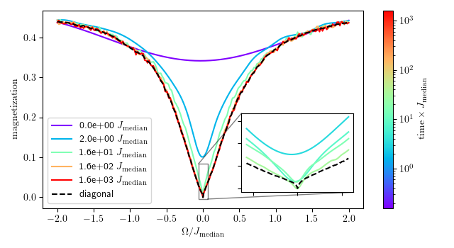
Figure 13: Similar to Fig. 11, Eigenstate expectation values of the magnetization for 9 different disorder realizations at $\Omega=-0.15J_{\mathrm{median}}$ and $r_{\mathrm{bl}}=0.1r_{\mathrm{max}}$ for all eigenstates as a function of eigenenergy. The color encodes the eigenstate occupation $|\innerproduct{\psi_{0}}{\phi_{\alpha}}|^{2}$.

The solid lines in Fig. 13 show the time-evolution of the magnetization, the time. At early times up to $\approx 10J_{\mathrm{median}}$, the magnetization depends smoothly on the external field $\Omega$, and the magnetization is strictly positive. After $\approx 10J_{\mathrm{median}}$, the dynamics without external fields have already almost reached a steady-state, whereas the magnetization continues to decrease if an external field is applied. As a result, the magnetization at $\approx 10J_{\mathrm{median}}$ features the steepest slope. In comparison, the steady-state, just like the diagonal ensemble, appears to be rather smooth apart from the small region within $|\Omega|<0.01J_{\mathrm{median}}$ showing the peaked structure.

This ambiguity concerning the existence of a cusp feature and hence thermalization shows most drastically when analyzing the eigenspectrum. Fig 14 shows the eigenstate expectation values and occupation numbers for 9 different disorder realizations for a dipolar interacting system with $r_{\mathrm{bl}}=0.1r_{\max}$. Interestingly, some realizations like realization 2, 3, and 5 show a scattered distribution of eigenstate expectation values which strongly resemble the strongly disordered case of Van-der-Waals interactions. These disorder realizations are inconsistent with ETH (condition (iii) in the main text). Contrary, other realizations, like realization 4, 7, and 8, exhibit a smooth dependence of the magnetization as a function of eigenenergy being compatible with ETH. In summary, we can’t conclude from the numeric simulations of only 14 dipolar interacting spins whether the system thermalizes or not. This uncertainty might be a consequence of the more long-range interactions with $a=d=3$, which generally favors thermalization.

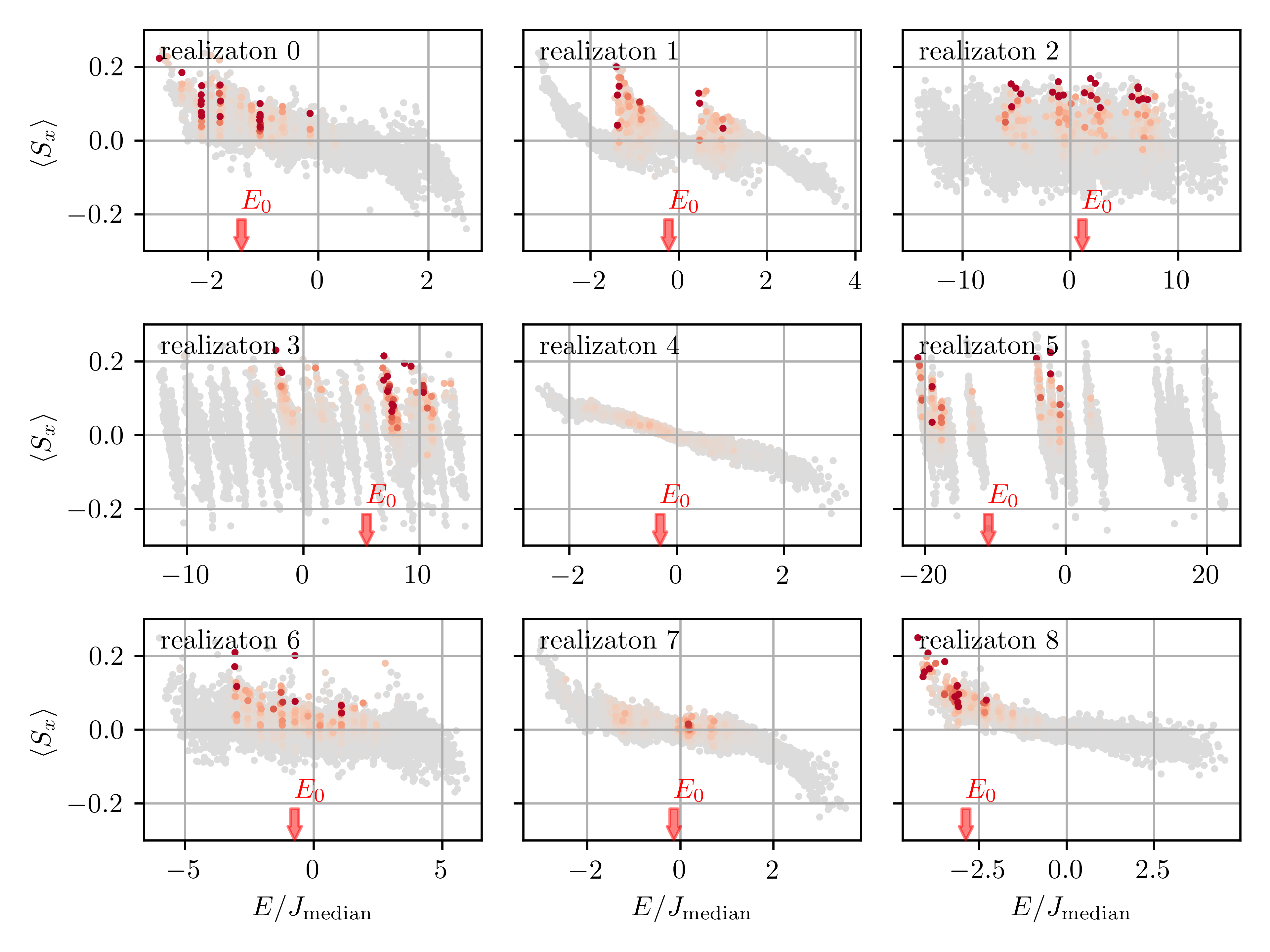
Figure 14: Similar to Fig. 11, Eigenstate expectation values of the magnetization for 9 different disorder realizations at $\Omega=-0.15J_{\mathrm{median}}$ and $r_{\mathrm{bl}}=0.1r_{\mathrm{max}}$ for all eigenstates as a function of eigenenergy. The color encodes the eigenstate occupation $|\innerproduct{\psi_{0}}{\phi_{\alpha}}|^{2}$.

Appendix H Mean-field model

It is often helpful to employ a mean-field approximation to obtain an intuitive understanding of the dynamics of interacting quantum systems. In this approximation, the Hamiltonian $\hat{H}_{\mathrm{int}}+\hat{H}_{\mathrm{iext}}$ becomes

$$\hat{H}_{\mathrm{mf}}=\sum_{i}\left(\left(\beta_{x}^{(i)}+\Omega\right)s_{x}^{(i)}+\beta_{y}^{(i)}s_{y}^{(i)}+\beta_{z}^{(i)}s_{z}^{(i)}\right)$$ (4)

where we defined the mean field $\beta_{\alpha}^{(i)}=\sum_{j}J_{ij}\langle\hat{s}_{\alpha}^{(j)}\rangle$ ($\alpha\in\left\{x,y,z\right\}$. Since the initial state is fully polarized in $x$-direction, the only non-zero component of the mean field is $\beta_{x}^{(i)}$ and the Hamiltonian simplifies to

$$\hat{H}_{\mathrm{mf}}=\sum_{i}\left(\beta_{x}^{(i)}+\Omega\right)s_{x}^{(i)}.$$ (5)

The resulting dynamics is a precession around the $x$-axis. Therefore in mean-field approximation, the initial state remains fully polarized and does not evolve at all, which is in stark contrast to the observed magnetization decay. Nonetheless, the mean-field picture provides an intuitive explanation for the asymmetry observed in the diagonal ensemble description of Fig. 1 c: For positive fields $\Omega$, the external field and the mean-field add up to a large effective field which leads to a strong spin locking effect. On the other hand, at small negative fields where $\Omega\approx-\beta_{x}^{(i)}$, the two components cancel each other, and the spin locking effect is diminished.

Appendix I Pair mean-field model

In this appendix, we introduce an approximation that remedies the shortcomings of the naive mean-field model by treating strongly interacting pairs of spins exactly and adding the effects of interactions between pairs on the mean-field level. This approximation provides an intuitive picture that allows us to explain all the observed features of the long-time magnetization (positivity, cusp, asymmetry).

For a single interacting pair, in the basis $\{\ket{\rightarrow\rightarrow},\ket{\rightarrow\leftarrow},\ket{\leftarrow\rightarrow},\ket{\leftarrow\leftarrow}\}$, Hamiltonian (2) reads

$$\hat{H}_{\mathrm{pair}} =2J\left(\Delta\hat{s}_{x}^{(1)}\hat{s}_{x}^{(2)}+\hat{s}_{y}^{(1)}\hat{s}_{y}^{(2)}+\hat{s}_{z}^{(1)}\hat{s}_{z}^{(2)}\right)+\Omega\sum_{i=1}^{2}\hat{s}_{z}^{(i)}$$ (6)

$$=\begin{pmatrix}J+\Omega&0&0&J(\Delta-1)\\ 0&-J&J(\Delta+1)&0\\ 0&J(\Delta+1)&-J&0\\ J(\Delta-1)&0&0&J-\Omega\end{pmatrix}$$ (7)

where we defined $J=J_{01}/4$. Out of the four eigenstates of this Hamiltonian, only two have non-zero overlap with the initial state $\ket{\rightarrow\rightarrow}$ (see table 2). Therefore, each interacting pair can be seen as an effective two-level system on its own, with a modified interaction between these "renormalized" spins. This ansatz of diagonalizing the strongest interacting pairs first can be seen as a first step in a real-space strong-disorder renormalization group treatment [20, 21, 22, 23]. Here, we do not aim to proceed further in this renormalization scheme, but instead, we use the basis of eigenstates of strongly interacting pairs to derive an intuitive understanding of the physics within mean-field theory.

Eigenvalue	Eigenvector	Occupation	Magnetization
$J\Delta$	$\dfrac{1\rule{0.0pt}{11.19443pt}}{\sqrt{2}\rule[-3.87495pt]{0.0pt}{0.0pt}}\left(\ket{\rightarrow\leftarrow}+\ket{\leftarrow\rightarrow}\right)$	0	0
$-J(2+\Delta)$	$\dfrac{1\rule{0.0pt}{11.19443pt}}{\sqrt{2}\rule[-3.87495pt]{0.0pt}{0.0pt}}\left(\ket{\rightarrow\leftarrow}-\ket{\leftarrow\rightarrow}\right)$	0	0
$J-\sqrt{\Omega^{2}+J^{2}\left(\Delta-1\right)^{2}}$	$\sqrt{\dfrac{1}{2}-\dfrac{\Omega}{2\sqrt{\Omega^{2}+j^{2}}}}\ket{\rightarrow\rightarrow}+\sqrt{\dfrac{1}{2}+\dfrac{\Omega}{2\sqrt{\Omega^{2}+j^{2}}}}\rule{0.0pt}{11.19443pt}\rule[-3.87495pt]{0.0pt}{0.0pt}\ket{\leftarrow\leftarrow}$	$\dfrac{1}{2}-\dfrac{\Omega}{2\sqrt{\Omega^{2}+j^{2}}}$	$-\dfrac{\Omega}{2\sqrt{\Omega^{2}+j^{2}}}$
$J+\sqrt{\Omega^{2}+J^{2}\left(\Delta-1\right)^{2}}$	$\sqrt{\dfrac{1}{2}+\dfrac{\Omega}{2\sqrt{\Omega^{2}+j^{2}}}}\ket{\rightarrow\rightarrow}+\sqrt{\dfrac{1}{2}-\dfrac{\Omega}{2\sqrt{\Omega^{2}+j^{2}}}}\rule{0.0pt}{11.19443pt}\rule[-3.87495pt]{0.0pt}{0.0pt}\ket{\leftarrow\leftarrow}$	$\dfrac{1}{2}+\dfrac{\Omega}{2\sqrt{\Omega^{2}+j^{2}}}$	$\dfrac{\Omega}{2\sqrt{\Omega^{2}+j^{2}}}$

Table 2: Properties of the four eigenstates of a single interacting spin pair. To simplify notation, we introduced $j=J\left(\Delta-1\right)$.

In contrast to a single spin which does not show any dynamics, a strongly interacting pair features oscillatory dynamics. Using the definition given in the main text, we can calculate the diagonal ensemble expectation value for single pair:

$$\overline{\langle\hat{S}_{x}\rangle_{\mathrm{pair}}}=\frac{\Omega^{2}}{2(\Omega^{2}+j^{2})}$$ (8)

where we introduced $j=J\left(\Delta-1\right)$. It should be noted that this diagonal ensemble does not describe the steady-state but rather the time average over the oscillations. The magnetization expectation value predicted by the diagonal ensemble of a single interacting pair represents an inverted Lorentz profile with width $j/2$, which features a quadratic dependence on $\Omega$ around zero (see Figure 15(a)). However, if we average over multiple pairs with different interaction strengths $j$, the diagonal ensemble value becomes more meaningful since we can assume that the different oscillation frequencies dephase. Also, the behavior of the magnetization changes: For example, assuming a uniform distribution of $j\in[0,\Delta_{j}]$, we obtain

$$\frac{1}{\Delta_{j}}\int_{0}^{\Delta_{j}}\overline{\langle\hat{S}_{x}\rangle_{\mathrm{pair}}}\,\mathrm{d}j=\frac{\Omega}{2\Delta_{j}}\arctan(\frac{\Delta_{j}}{\Omega})$$ (9)

which shows the non-analytic cusp feature at $\Omega=0$ (see Figure 15(b)). Close to the non-analytic point, the magnetization increases linearly with a slope $\dfrac{\pi}{4\Delta_{j}}$ inversely proportional to the width of the distribution of interaction strengths. Therefore, we can conclude that the non-analyticity is a direct consequence of disorder and the resulting broad distribution of nearest neighbor interaction strengths.

To obtain an even more realistic model and to understand additional features like the asymmetry, we add a mean-field interaction between pairs. For this purpose, we replace the external field with an effective mean-field acting on spin $i$:

$$\Omega\rightarrow\Omega_{i}=\Omega+\sum_{j}J_{ij}^{\mathrm{inter}}\langle\hat{s}_{x}^{(j)}\rangle$$ (10)

As a first example, we may consider a periodic chain of equally spaced pairs where all pairs are identical and the mean-field shift arising from interactions between the pairs is $J^{\mathrm{inter}}$. In this case, the diagonal ensemble expectation value can be calculated by solving the self-consistent equation

$$\overline{\langle\hat{S}_{x}\rangle}=\frac{1}{2}\frac{\left(\Omega+J^{\mathrm{inter}}\overline{\langle\hat{S}_{x}\rangle}\right)^{2}}{\left(\Omega+J^{\mathrm{inter}}\overline{\langle\hat{S}_{x}\rangle}\right)^{2}+j^{2}}.$$ (11)

Since the right-hand side of the equation only contains squares, the magnetization is still positive or zero. Therefore, for positive external fields $\Omega$, the effective field is larger than the external field ($\Omega_{i}\geq\Omega$), leading to an enhanced spin locking effect. Consequently, mean-field leads to an increased magnetization compared to the case of independent pairs. For negative $\Omega$, the external field is anti-aligned with the mean-field, and the resulting magnetization is decreased. Thus, the dependence of the magnetization as a function of field strength is asymmetric (see Figure 15(c)). In conclusion, we can attribute the asymmetry to mean-field interaction between different pairs.

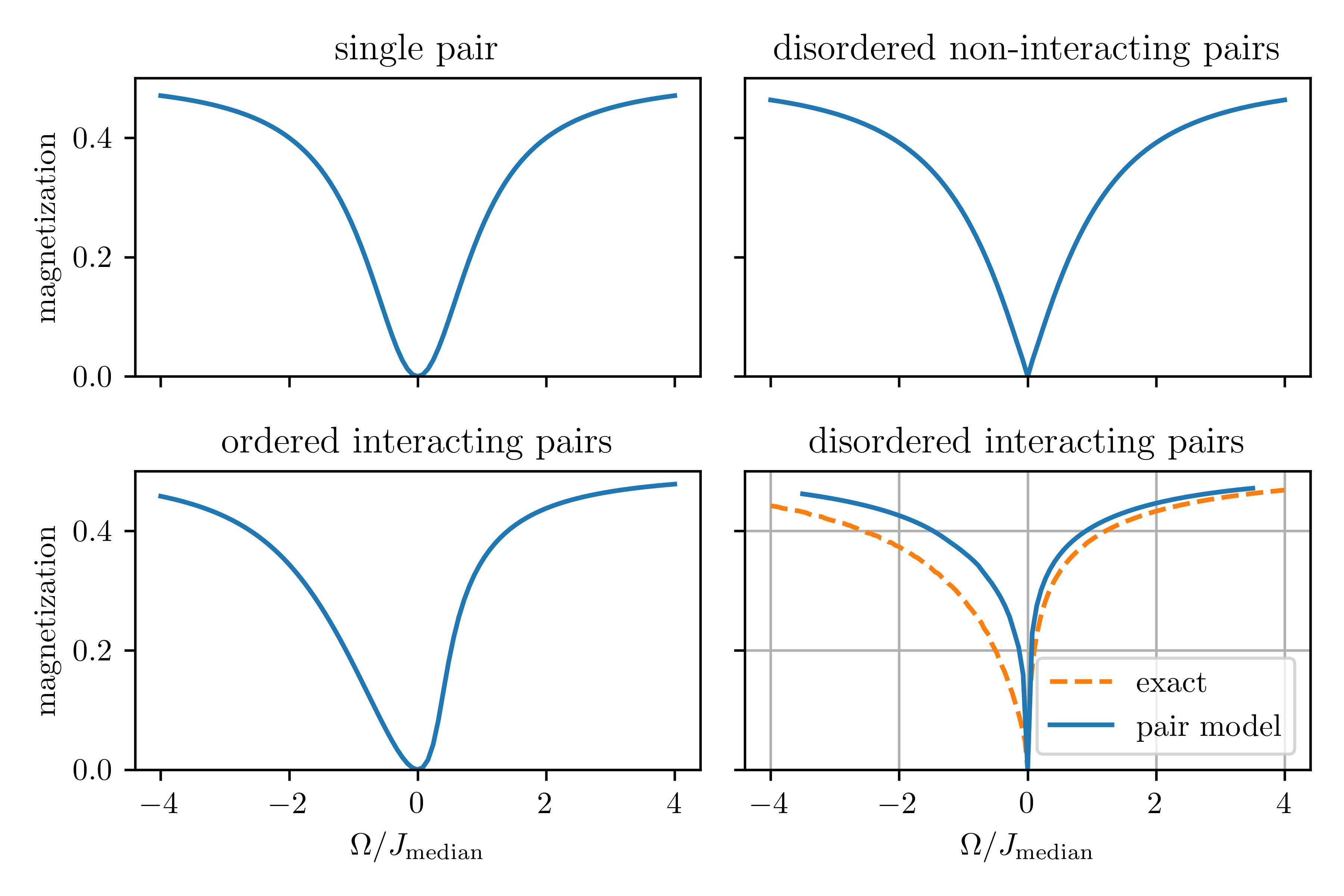
Figure 15: The diagonal ensemble expectation value of the magnetization as a function of applied external field $\Omega$ for (a) a single pair, (b) a disorder average of single pairs with interaction chosen randomly in the interval $J\in[0,1]$, (c) a system of identical pairs that interact with mean field interaction $J_{\mathrm{inter}}=1.5*J$, and (d) a realistic random distribution with power-law interactions, as described in the text. For the latter, the dashed orange line shows the full quantum mechanical solution obtained by exact diagonalization for the same system.

In order to model the disordered spin system realized experimentally, we apply the pair model to an ensemble of spins with randomly chosen positions. We cluster the spins $i$ into pairs $p$ in such a way that the sum over all pair distances is minimized. Naturally, the interaction $j_{p}$ of a pair $p$ consisting of spins $i$ and $j$ is given by the interaction strength between the spins. The interaction strength $J_{pq}^{\mathrm{inter}}$ between pair $p$ and $q$ can be obtained from the strongest interaction $J_{ij}$ where spin $i$ is in pair $p$ and $j$ in $q$ respectively. Now, we solve the system of self-consistent equations

$$\overline{\langle\hat{s}_{x}^{p}\rangle}=\frac{1}{2}\frac{\left(\Omega+\sum_{q}(J_{pq}^{\mathrm{inter}}\overline{\langle\hat{s}_{x}^{q}\rangle})\right)^{2}}{\left(\Omega+\sum_{q}(J_{pq}^{\mathrm{inter}}\overline{\langle\hat{s}_{x}^{q}\rangle})\right)^{2}+j_{p}^{2}}.$$ (12)

The resulting magnetization curve obtained after disorder averaging (see blue line in Figure 15(d)) closely resembles the exact diagonal ensemble prediction (orange line). Importantly, all qualitative features are captured, including a positive magnetization which is asymmetric with respect to the external field and shows a sharp cusp at zero field. The remaining discrepancy between the pair model and the exact solution, in particular the stronger asymmetry of the exact solution, can be attributed to clusters of spins containing more than two atoms where quantum fluctuations decrease the magnetization even further than predicted by the pair mean-field model.

We conclude that the heuristic pair mean-field model provides an intuitive understanding of the diagonal ensemble prediction. Furthermore, we can also apply it to investigate the microcanonical ensemble. To this end, we assume that the microcanonical ensemble expectation value is determined solely by the eigenstate closest in energy to the energy $E_{0}$ of the initial state. Without mean-field interaction, the energy of the system $E_{0}$ is closer to the upper eigenstate featuring positive magnetization for positive fields (respectively closer to the lower eigenstate for negative fields) (see Figure 16 (a and b). Thus, $E_{0}$ is always closer to the positively polarized eigenstate and we expect a positive magnetization for the microcanonical ensemble for all field values $\Omega$. This changes when we take into account the mean-field interaction between pairs. Due to the assumption that the system is exactly in a single eigenstate, we can calculate the magnetization of each eigenstate via the self-consistent equation

$$\langle\hat{s}_{x}\rangle_{\pm}=\pm\dfrac{\Omega+J^{\mathrm{inter}}\langle\hat{s}_{x}\rangle_{\pm}}{2\sqrt{(\Omega+J^{\mathrm{inter}}\langle\hat{s}_{x}\rangle_{\pm})^{2}+j^{2}}}\,.$$ (13)

The resulting effective field $\Omega+J^{\mathrm{inter}}\langle\hat{s}_{x}\rangle_{\pm}$ changes the eigenvalues, and the spectrum becomes asymmetric with respect to the lower and upper branch. Most strikingly, a region of small negative fields exists where the energy of the system $E_{0}$ is closer to the upper eigenstate which features a negative magnetization (compare the dashed gray line showing $E_{0}$ with the solid gray line showing the center between the eigenstates in Figure 16 (c and d)). This explains why the magnetization of the microcanonical ensemble can become negative for small negative $\Omega$.

Comparing this model to a many-body spectrum obtained by exact diagonalization of the full quantum mechanical Hamiltonian, we notice that the highest and lowest excited states show the same features as the two eigenstates of a single pair in the mean-field model. Additionally, in between these two states, we find a plethora of further eigenstates. In a microcanonical description, the eigenstates closest to the energy of the system are populated. Therefore, for small negative fields, the microcanonical ensemble populates states which are closer in energy to the highest excited state. Since these states typically feature negative magnetization, we obtain a negative magnetization for the microcanonical ensemble similar to the red line in Figure 1 c in the main text.

The right column of Figure 16 also shows the eigenstate occupation for each of the studies systems. Notably, we can see that not only the eigenstates closest in energy to $E_{0}$ are populated. Rather, the occupation is highly correlated with the magnetization of the eigenstate. Therefore, the assumption of the microcanonical ensemble is not justified leading to the qualitative different behavior of the microcanonical and diagonal ensembles.

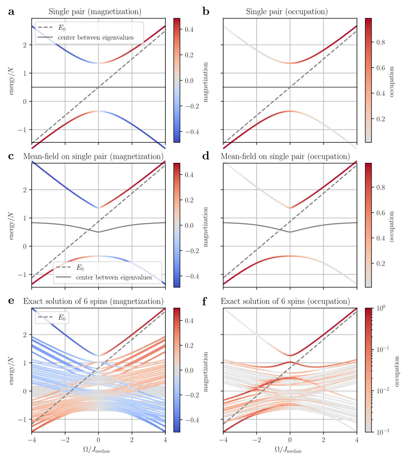
Figure 16: Eigenvalue spectra and eigenstate properties for pairs of spins compared to properties of the full many-body spectrum. In the left column, the color gradient encodes the magnetization of each eigenstate. In the right column, the color gradient represents the wavefunction overlap of the eigenstate with the initial state of fully $x$-polarized spins. Panels a and b show the eigenstate properties of a single pair given in Table 2. Panels c and d show the eigenstates of a pair including the mean-field shift caused by the surrounding pairs according to eq. (13). The full many-body spectrum of a disordered system of $N=6$ spins is shown in panels e and f. The qualitative correspondence between the middle row and the extremal states in the lower row is clearly visible, showing that the pair mean-field picture may provide an intuitive understanding of the properties of the many-body spectrum.

Appendix J Finite size scaling

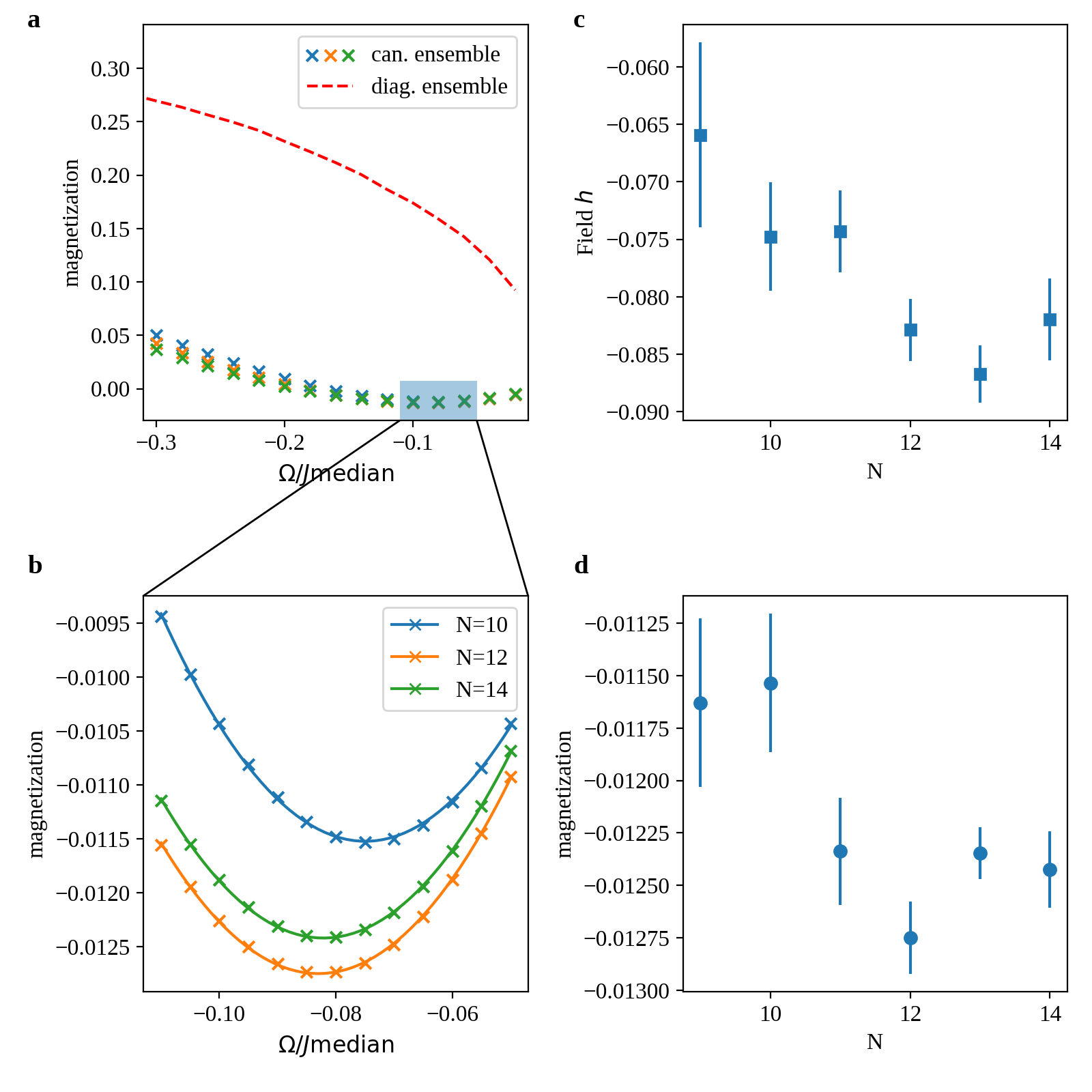
Figure 17: Finite size scaling methodology. a, shows an overview of diagonal and canonical ensembles. We obtain detailed data (b) around the minima for different $N$ and perform a quadratic fit to extract the position (c) and depth (d) of the minima.

To strengthen confidence in our results, we perform finite-size scaling on a one-dimensional system with periodic boundary conditions (at $r_{b}=0.5r_{\mathrm{max}}$ with van-der-Waals interactions). This analysis shows that the main qualitative difference between diagonal and thermal ensembles, being the thermal ensembles’ dip below zero magnetization at small negative field strength, appears to be stable. Figure 17 c and 17 d show that the position and depth of the minimum are not yet perfectly converged but seems to stabilize around at small negative values. There is no clear drift visible, meaning the thermal ensembles minimum is indeed negative and at small negative external field.

References

- Deutsch [1991] J. M. Deutsch, Physical Review A 43, 2046 (1991).
- Srednicki [1999] M. Srednicki, Journal of Physics A , 14 (1999).
- Srednicki [1994] M. Srednicki, Physical Review E 50, 888 (1994).
- Nandkishore and Huse [2015] R. Nandkishore and D. A. Huse, Annual Review of Condensed Matter Physics 6, 15 (2015).
- Abanin et al. [2019] D. A. Abanin, E. Altman, I. Bloch, and M. Serbyn, Reviews of Modern Physics 91, 021001 (2019).
- Browaeys and Lahaye [2020] A. Browaeys and T. Lahaye, Nature Physics 16, 132 (2020).
- Signoles et al. [2021] A. Signoles, T. Franz, R. Ferracini Alves, M. Gärttner, S. Whitlock, G. Zürn, and M. Weidemüller, Physical Review X 11, 011011 (2021).
- Geier et al. [2021] S. Geier, N. Thaicharoen, C. Hainaut, T. Franz, A. Salzinger, A. Tebben, D. Grimshandl, G. Zürn, and M. Weidemüller, Science 374, 1149 (2021).
- Mori et al. [2018] T. Mori, T. N. Ikeda, E. Kaminishi, and M. Ueda, Journal of Physics B: Atomic, Molecular and Optical Physics 51, 112001 (2018).
- De Roeck and Huveneers [2017] W. De Roeck and F. Huveneers, Physical Review B 95, 155129 (2017).
- Morningstar et al. [2022] A. Morningstar, L. Colmenarez, V. Khemani, D. J. Luitz, and D. A. Huse, Physical Review B 105, 174205 (2022).
- Sels and Polkovnikov [2022] D. Sels and A. Polkovnikov, “Thermalization of dilute impurities in one dimensional spin chains,” (2022), arXiv:2105.09348 [cond-mat, physics:quant-ph] .
- Luitz et al. [2017] D. J. Luitz, F. Huveneers, and W. De Roeck, Physical Review Letters 119, 150602 (2017).
- Ponte et al. [2017] P. Ponte, C. R. Laumann, D. A. Huse, and A. Chandran, Philosophical Transactions of the Royal Society A: Mathematical, Physical and Engineering Sciences 375, 20160428 (2017).
- Thiery et al. [2018] T. Thiery, F. Huveneers, M. Müller, and W. De Roeck, Physical Review Letters 121, 140601 (2018).
- Burin [2006] A. L. Burin, “Energy delocalization in strongly disordered systems induced by the long-range many-body interaction,” (2006), arXiv:cond-mat/0611387 .
- Yao et al. [2014] N. Y. Yao, C. R. Laumann, S. Gopalakrishnan, M. Knap, M. Müller, E. A. Demler, and M. D. Lukin, Physical Review Letters 113, 243002 (2014).
- Gutman et al. [2016] D. B. Gutman, I. V. Protopopov, A. L. Burin, I. V. Gornyi, R. A. Santos, and A. D. Mirlin, Physical Review B 93, 245427 (2016).
- Abanin et al. [2021] D. A. Abanin, J. H. Bardarson, G. De Tomasi, S. Gopalakrishnan, V. Khemani, S. A. Parameswaran, F. Pollmann, A. C. Potter, M. Serbyn, and R. Vasseur, Annals of Physics 427, 168415 (2021).
- Pekker et al. [2014] D. Pekker, G. Refael, E. Altman, E. Demler, and V. Oganesyan, Physical Review X 4, 011052 (2014).
- Vasseur et al. [2016] R. Vasseur, A. J. Friedman, S. A. Parameswaran, and A. C. Potter, Physical Review B 93, 134207 (2016).
- Vasseur et al. [2015] R. Vasseur, A. C. Potter, and S. A. Parameswaran, Physical Review Letters 114, 217201 (2015).
- Vosk and Altman [2013] R. Vosk and E. Altman, Physical Review Letters 110, 067204 (2013).
- Bloch et al. [2008] I. Bloch, J. Dalibard, and W. Zwerger, Reviews of Modern Physics 80, 885 (2008).
- Esslinger [2010] T. Esslinger, Annual Review of Condensed Matter Physics 1, 129 (2010).
- Bloch et al. [2012] I. Bloch, J. Dalibard, and S. Nascimbène, Nature Physics 8, 267 (2012).
- Gross and Bloch [2017] C. Gross and I. Bloch, Science 357, 995 (2017).
- Schreiber et al. [2015] M. Schreiber, S. S. Hodgman, P. Bordia, H. P. Lüschen, M. H. Fischer, R. Vosk, E. Altman, U. Schneider, and I. Bloch, Science 349, 842 (2015).
- Bordia et al. [2016] P. Bordia, H. P. Lüschen, S. S. Hodgman, M. Schreiber, I. Bloch, and U. Schneider, Physical Review Letters 116, 140401 (2016).
- Choi et al. [2016] J.-y. Choi, S. Hild, J. Zeiher, P. Schauß, A. Rubio-Abadal, T. Yefsah, V. Khemani, D. A. Huse, I. Bloch, and C. Gross, Science 352, 1547 (2016).
- Smith et al. [2016] J. Smith, A. Lee, P. Richerme, B. Neyenhuis, P. W. Hess, P. Hauke, M. Heyl, D. A. Huse, and C. Monroe, Nature Physics 12, 907 (2016).
- Kaufman et al. [2016] A. M. Kaufman, M. E. Tai, A. Lukin, M. Rispoli, R. Schittko, P. M. Preiss, and M. Greiner, Science 353, 794 (2016).
- Lukin et al. [2019] A. Lukin, M. Rispoli, R. Schittko, M. E. Tai, A. M. Kaufman, S. Choi, V. Khemani, J. Léonard, and M. Greiner, Science 364, 256 (2019).
- Léonard et al. [2020] J. Léonard, M. Rispoli, A. Lukin, R. Schittko, S. Kim, J. Kwan, D. Sels, E. Demler, and M. Greiner, (2020).
- Gogolin and Eisert [2016] C. Gogolin and J. Eisert, Reports on Progress in Physics 79, 056001 (2016).
- Rigol et al. [2008] M. Rigol, V. Dunjko, and M. Olshanii, Nature 452, 854 (2008).
- Linden et al. [2009] N. Linden, S. Popescu, A. J. Short, and A. Winter, Physical Review E 79, 061103 (2009).
- Schultzen et al. [2022a] P. Schultzen, T. Franz, S. Geier, A. Salzinger, A. Tebben, C. Hainaut, G. Zürn, M. Weidemüller, and M. Gärttner, Physical Review B 105, L020201 (2022a).
- Schultzen et al. [2022b] P. Schultzen, T. Franz, C. Hainaut, S. Geier, A. Salzinger, A. Tebben, G. Zürn, M. Gärttner, and M. Weidemüller, Physical Review B 105, L100201 (2022b).
- Günther [2013] H. Günther, NMR Spectroscopy: Basic Principles, Concepts and Applications in Chemistry, third, completely revised and updated edition ed. (Wiley-VCH, Weinheim, 2013).
- Serbyn et al. [2013] M. Serbyn, Z. Papić, and D. A. Abanin, Physical Review Letters 111, 127201 (2013).
- Huse et al. [2014] D. A. Huse, R. Nandkishore, and V. Oganesyan, Physical Review B 90, 174202 (2014).
- Imbrie [2016] J. Z. Imbrie, Journal of Statistical Physics 163, 998 (2016).
- Defenu et al. [2015] N. Defenu, A. Trombettoni, and A. Codello, Physical Review E 92, 052113 (2015).
- Millán et al. [2021] A. P. Millán, G. Gori, F. Battiston, T. Enss, and N. Defenu, Physical Review Research 3, 023015 (2021).
- Álvarez et al. [2015] G. A. Álvarez, D. Suter, and R. Kaiser, Science 349, 846 (2015).
- Waldherr et al. [2014] G. Waldherr, Y. Wang, S. Zaiser, M. Jamali, T. Schulte-Herbrüggen, H. Abe, T. Ohshima, J. Isoya, J. F. Du, P. Neumann, and J. Wrachtrup, Nature 506, 204 (2014).
- Yan et al. [2013] B. Yan, S. A. Moses, B. Gadway, J. P. Covey, K. R. A. Hazzard, A. M. Rey, D. S. Jin, and J. Ye, Nature 501, 521 (2013).
- de Paz et al. [2013] A. de Paz, A. Sharma, A. Chotia, E. Maréchal, J. H. Huckans, P. Pedri, L. Santos, O. Gorceix, L. Vernac, and B. Laburthe-Tolra, Phys. Rev. Lett. 111, 185305 (2013).
- Baier et al. [2016] S. Baier, M. J. Mark, D. Petter, K. Aikawa, L. Chomaz, Z. Cai, M. Baranov, P. Zoller, and F. Ferlaino, Science 352, 201 (2016).
- Ferreira-Cao et al. [2020] M. Ferreira-Cao, V. Gavryusev, T. Franz, R. F. Alves, A. Signoles, G. Zürn, and M. Weidemüller, Journal of Physics B: Atomic, Molecular and Optical Physics 53, 084004 (2020).
- Weimer et al. [2008] H. Weimer, R. Löw, T. Pfau, and H. P. Büchler, Physical Review Letters 101, 250601 (2008).
- Gärttner et al. [2012] M. Gärttner, K. P. Heeg, T. Gasenzer, and J. Evers, Physical Review A 86, 033422 (2012).
- Orioli et al. [2018] A. P. Orioli, A. Signoles, H. Wildhagen, G. Günter, J. Berges, S. Whitlock, and M. Weidemüller, Physical Review Letters 120, 063601 (2018).
- Schachenmayer et al. [2015] J. Schachenmayer, A. Pikovski, and A. M. Rey, Physical Review X 5, 011022 (2015).
- Amthor et al. [2010] T. Amthor, C. Giese, C. S. Hofmann, and M. Weidemüller, Physical Review Letters 104, 013001 (2010).