Endpoint factorization and next-to-leading power resummation of gluon thrust

Abstract

Endpoint divergences in the convolution integrals appearing in next-to-leading-power factorization theorems prevent a straightforward application of standard methods to resum large logarithmic power-suppressed corrections in collider physics. We study the power-suppressed configuration of the thrust distribution in the two-jet region, where a gluon-initiated jet recoils against a quark-antiquark pair. With the aid of operatorial endpoint factorization conditions, we derive a factorization formula where the individual terms are free from endpoint divergences and can be written in terms of renormalized hard, (anti) collinear, and soft functions in four dimensions. This framework enables us to perform the first resummation of the endpoint-divergent SCET_I observables at the leading logarithmic accuracy using exclusively renormalization-group methods.

1 Introduction

The endpoint factorization and next-to-leading power (NLP) resummation of gluon thrust employing renormalization group (RG) methods has recently been presented in [1]. This proceeding highlights the key insights alongside showcasing the main results. For precise definitions and technicalities of the derivation, we direct the interested reader to the original publication.

In the past, hadronic event shape variables in the two-jet region were of great importance in the development of diagrammatic resummation methods for QCD [2, 3]. Later, the advent of soft-collinear effective theory (SCET) enabled the accuracy of resummation to be further improved. This was first shown for the thrust variable $T$ [4], defined as

$$T=\mbox{max}_{\vec{n}}\,\frac{\sum_{i}\left|\vec{p_{i}}\cdot\vec{n}\right|}{\sum_{i}\left|\vec{p_{i}}\right|},$$ (1)

where the index $i$ sums over all final state hadrons (partons). As $\tau=1-T\to 0$,  back-to-back jets are formed by the particles, and large logarithms $\ln\tau$ appear at every order in $\alpha_{s}$, signalling a breakdown in perturbation theory. This phenomenon has been scrutinized in great detail for the quark-antiquark two-jet process that contributes at leading power (LP) in the $\tau$ expansion.

In the work presented here, we instead focus on the “gluon thrust” phase-space region where at leading order (LO) the gluon recoils a quark-antiquark pair

$$e^{+}e^{-}\to\gamma^{*}\to[g]_{c}+[q\bar{q}]_{\bar{c}}\,.$$ (2)

The gluon and the quark-antiquark jets are chosen to be in the collinear and anticollinear directions, respectively. As shown in figure 1, this process begins at $\mathcal{O}(\alpha_{s})$ and it is of particular interest in our investigations as in the limit of $\tau\to 0$ the LP $[\ln\tau/\tau]_{+}$ soft-gluon behaviour is absent. Instead, the process begins at NLP in the $\tau$ expansion, with the leading term being $\alpha_{s}\ln\tau$.

The study of power corrections in a multitude of contexts has recently gathered considerable attention. However, as we discuss below, further rapid progress has thus far been hindered by the ubiquitous appearance of endpoint divergences in convolution integrals between the hard, (anti-) collinear, and soft functions in the NLP factorization theorems, such as for the Drell-Yan threshold [5]. We address this key conceptual issue in the context of gluon thrust, as it allows us to focus on the problem of endpoint divergences without needing to address additional difficulties such as factorization of parton distribution functions, which would affect Drell-Yan and DIS processes.

The result for the all-order logarithmic structure of “gluon thrust” at the double logarithmic (DL) accuracy was first written down in [6] and later derived from $d$-dimensional consistency relations in [7]. An interesting feature of this result is the unconventional “quark” Sudakov form factor, which arises due to the colour mismatch between the back-to-back energetic particles when either the quark or anti-quark in the $q\bar{q}$-jet becomes soft, causing the double logarithms to be proportional to the difference of the colour charges, $C_{A}-C_{F}$. Despite the progress in the description of this process within SCET [6, 8, 7], it has not yet been possible to improve the resummation accuracy beyond DL order due to the presence of endpoint-divergences in the relevant convolution integrals.

In this work, we develop the refactorization ideas employed for the DIS process [7], and Higgs decay to two photons through light-quark loops [9, 10] in order to derive a SCET_I NLP factorization theorem valid in $d=4$ dimensions. To arrive at this result, we make use of standard factorization within SCET combined with endpoint factorization.

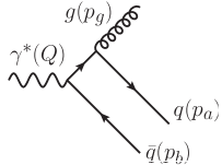
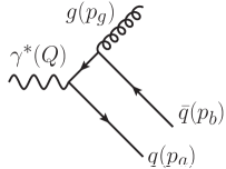
Figure 1: Diagrams contributing to gluon thrust at leading $\alpha_{s}$ order in QCD.

2 Heuristic discussion

In this section, we present a sketch of the factorization formula in the EFT framework, which aids in motivating the endpoint rearrangement and subtraction terms introduced below. At $\mathcal{O}(\alpha_{s})$, there are two ways to induce the gluon jet:

1. Both the quark and the anti-quark can carry large anti-collinear momentum and create a single jet recoiling against the collinear gluon.

2. Either the quark or the anti-quark is anti-collinear and balances the collinear gluon momentum, in which case the other fermion is soft.

Both situations provide identical power suppression in $\tau$, and the further evolution of the process is governed by LP interactions. However, the separation into possibilities I and II introduces an ambiguity in what is precisely meant by the “soft” and “anti-collinear” modes. If we begin with configuration I and lower the large anti-collinear momentum of either the quark or the anti-quark, eventually it will become soft, at which point it should in fact be counted as a contribution to situation II rather than I. As long as the definition of the jet is infrared safe, this separation is not an issue for fixed-order computations. It is a problem, however, if the goal is to perform resummation since, in this case, a clear separation of soft and (anti) collinear modes is required in order to disentangle large logarithms into single-scale pieces. This tension between the mathematical description of the modes and the physical picture is the origin of the endpoint-divergences which appear in convolution integrals of the NLP factorization theorems.

We now focus on the Feynman diagrams in figure 1 and analyze possibilities I and II from the point of view of SCET. Starting with I, later referred to as “B-type”, we see that the internal propagator in the left diagram carries hard momentum $q_{a}=p_{g}+p_{a}$ (since $p_{g}$ is collinear and $p_{a}$ anti-collinear). As the intermediate propagator is hard, $q_{a}^{2}\sim Q^{2}$, it is integrated out, and the hard scattering vertex in SCET directly produces a $q\bar{q}g$ state. This is shown in the left-most diagram of figure 2. Only the total momentum of the $q\bar{q}$ anti-collinear pair is fixed by momentum conservation, while the amplitude depends on the fraction of the momentum carried by each particle. In the case where one of these fractions becomes vanishingly small, the corresponding parton is effectively soft and should be counted as possibility II, which we later refer to as the “A-type” contribution. Here, the $q_{a}$-intermediate propagator, or $q_{b}$ for the soft anti-quark case, ceases to be hard. Therefore, the hard scattering vertex is the LP $\gamma^{*}\to q\bar{q}$ process and the entire momentum of the energetic quark (or anti-quark) is subsequently transferred to the gluon, rendering the daughter fermion soft. In SCET, such a situation is described by an insertion of a power-suppressed SCET Lagrangian interaction term $\mathcal{L}^{(1)}_{\xi q}$, which constitutes soft (anti-) quark emission, as depicted in the middle and right-most diagrams of figure 2.

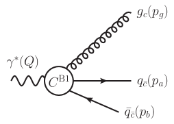
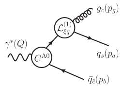
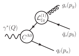
Figure 2: Representation of the gluon-thrust amplitude in the two-jet region in SCET.

The fact that there exists an overlap region where the limits of two different expressions can describe the same physical process is central to the idea of endpoint factorization. Before we make these concepts concrete, let us start with the following schematic discussion. In Laplace space, the factorization theorem for two-hemisphere invariant mass distribution of gluon thrust takes the following form:

$$\frac{1}{\sigma_{0}}\frac{\widetilde{d\sigma}}{ds_{R}ds_{L}} =\int_{0}^{\Lambda}d\omega d\omega^{\prime}\,\left|C^{A0}\right|^{2}\times\mathcal{J}^{(\bar{q})}_{\bar{c}}\times\mathcal{J}_{c}\left(\omega,\omega^{\prime}\right)\otimes S_{\rm NLP}\left(\omega,\omega^{\prime}\right)$$

$$+\int_{\Lambda/Q}^{1-\Lambda/Q}drdr^{\prime}\,C^{B1}(r)C^{B1}(r^{\prime})^{*}\otimes\mathcal{J}^{q\bar{q}}_{\bar{c}}\left(r,r^{\prime}\right)\times\mathcal{J}_{c}^{(g)}\times S^{(g)}\,.$$ (3)

In this formula, the hard matching coefficients are denoted by $C$, the jet functions by $\mathcal{J}$ and the soft functions by $S$. In the arguments of functions, we only retain the dependence on convolution variables which contain divergent integrals. The $\omega$ and $\omega^{\prime}$ soft-collinear convolutions diverge logarithmically for $\omega,\omega^{\prime}\to\infty$, and the $r$, $r^{\prime}$ hard-anti-collinear convolution integrals are logarithmically divergent for $r,r^{\prime}\to 0,1$.

The soft function $S_{\rm NLP}$ contains the soft quark from situation II. In the overlap region, this soft quark carries a large soft momentum $\omega$ and could be thought of as being a part of the $\mathcal{J}^{q\bar{q}}_{\bar{c}}$ anti-collinear function appearing in the bottom line of (3), with a small anti-collinear momentum fraction $r$. Taking away this quark from $S_{\rm NLP}$ leaves behind only $S^{(g)}$, therefore in total $S_{\rm NLP}\to S^{(g)}$, $\mathcal{J}^{(\bar{q})}_{\bar{c}}\to\mathcal{J}^{q\bar{q}}_{\bar{c}}$, and the hard process changes from A0-type to B1-type. Hence, in these limits, the integrands of the two terms in (3) should be identical. This fact allows us, in the singular limits, to perform a rearrangement at the integrand level, such that both terms are individually finite. At this stage, we can employ standard RG techniques to resum the logarithms in the hard, jet, and soft functions, as we show in more detail in the following sections.

3 Bare factorization theorem

Before focusing on endpoint factorization, we state the results of the derivation of the $d$-dimensional SCET factorization formula for gluon thrust [1]. To start, we integrate out the hard modes and match the electromagnetic current to

$$\bar{\psi}\gamma_{\perp}^{\mu}\psi(0) = \int dtd\bar{t}\,\widetilde{C}^{\rm A0}(t,\bar{t})\,\bar{\chi}_{c}(tn_{+})\gamma_{\perp}^{\mu}\chi_{\bar{c}}(\bar{t}n_{-})+(c\leftrightarrow\bar{c})$$ (4)

$$+\,\sum_{i=1,2}\int dtd\bar{t}_{1}d\bar{t}_{2}\,\widetilde{C}^{\rm B1}_{i}(t,\bar{t}_{1},\bar{t}_{2})\,\bar{\chi}_{\bar{c}}(\bar{t}_{1}n_{-})\Gamma_{i}^{\mu\nu}\mathcal{A}_{c\perp\nu}(tn_{+})\chi_{\bar{c}}(\bar{t}_{2}n_{-})+\ldots\qquad$$

In the first line, we have the LP hard scattering vertex, which produces a back-to-back quark-antiquark pair. It contributes to gluon thrust through a time-ordered product with the $\mathcal{O}(\lambda)$ suppressed SCET Lagrangian [11] term

$$\mathcal{L}_{\xi q}(x)=\bar{q}_{s}(x_{-})\not{\mathcal{A}}_{c\perp}(x)\chi_{c}(x)+\rm{h.c.}\,,$$ (5)

which transforms a collinear quark into a collinear gluon and a soft quark. The soft quark argument $x_{\mp}^{\mu}$ is defined as $x_{\mp}^{\mu}=(n_{\pm}\cdot x)\frac{n_{\mp}^{\mu}}{2}$. In the second line of (4), we have the $\mathcal{O}(\lambda)$ suppressed “B-type” SCET operator, which produces a collinear gluon and an anti-collinear quark-antiquark pair directly, see the left-most diagram in figure 2. The relevant Dirac structures in the B-type operator are

$$\Gamma_{1}^{\mu\nu}=\frac{\not{n}_{-}}{2}\gamma_{\perp}^{\nu}\gamma_{\perp}^{\mu}\,,\qquad\quad\Gamma_{2}^{\mu\nu}=\frac{\not{n}_{-}}{2}\gamma_{\perp}^{\mu}\gamma_{\perp}^{\nu}\,.$$ (6)

The remaining steps of the derivation are fairly standard. The collinear, anti-collinear and soft fields are decoupled at LP by the redefinition of the collinear field with the soft Wilson line [12] $Y_{n_{-}}(x)=\mathcal{P}\exp\left[ig_{s}\int_{0}^{\infty}dsn_{-}A_{s}(x+sn_{-})\right]$. We then square the matrix elements, sum and integrate over all possible final states. Since the final state $|X\rangle=|X_{c}\rangle|X_{\bar{c}}\rangle|X_{s}\rangle$ is made up of corresponding modes, the matrix element factorizes into collinear, anti-collinear and soft functions. Following this prescription for the two terms in (4) gives rise to the A-type and B-type contributions to the factorization formula, for which we present the results separately. We give results for the two-hemisphere invariant-mass distribution, which is related to the thrust distribution by

$$\frac{d\sigma}{d\tau}=\int dM_{R}^{2}dM_{L}^{2}\,\delta\!\left(\tau-\frac{M_{R}^{2}+M_{L}^{2}}{Q^{2}}\right)\frac{d\sigma}{dM_{R}^{2}dM_{L}^{2}}\,.$$ (7)

For the A-type contribution we find

$$\frac{1}{\sigma_{0}}\frac{d\sigma}{dM_{R}^{2}dM_{L}^{2}}|_{\rm A-type} = \frac{2C_{F}}{Q}\,f(\epsilon)\,|C^{\rm A0}(Q^{2})|^{2}\int_{0}^{\infty}dl_{+}dl_{-}\,\int d\omega d\omega^{\prime}\,\mathcal{J}_{\bar{c}}^{(\bar{q})}(M_{R}^{2}-Ql_{+})$$ (8)

$$\times\,\bigg{\{}\,\mathcal{J}_{c}(M_{L}^{2}-Ql_{-},\omega,\omega^{\prime})\,S_{\rm NLP}(l_{+},l_{-},\omega,\omega^{\prime})+\,\widehat{\mathcal{J}}_{c}(M_{L}^{2}-Ql_{-},\omega,\omega^{\prime})\,\widehat{S}_{\rm NLP}(l_{+},l_{-},\omega,\omega^{\prime})\,\bigg{\}}\,,$$

and for the B-type

$$\frac{1}{\sigma_{0}}\frac{d\sigma}{dM_{R}^{2}dM_{L}^{2}}|_{\rm B-type} = \frac{2C_{F}}{Q^{2}}\,f(\epsilon)\int_{0}^{\infty}dl_{+}dl_{-}\,\sum_{i,i^{\prime}=1,2}\int drdr^{\prime}\,C^{\rm B1*}_{i^{\prime}}(Q^{2},r^{\prime})C^{\rm B1}_{i}(Q^{2},r)$$

$$\times\bigg{\{}\delta_{ii^{\prime}}\mathcal{J}_{\bar{c}}^{q\bar{q}(8)}(M_{R}^{2}-Ql_{+},r,r^{\prime})+(1-\delta_{ii^{\prime}})\mathcal{\widehat{J}}_{\bar{c}}^{q\bar{q}(8)}(M_{R}^{2}-Ql_{+},r,r^{\prime})\bigg{\}}\mathcal{J}_{c}^{(g)}(M_{L}^{2}-Ql_{-})\,S^{(g)}(l_{+},l_{-})\,.$$

In the above equations, $f(\epsilon)$ is a $d$-dimensional factor with $f(0)=1$ in four dimensions. The precise operator definitions for all the functions, along with the lowest-order results, can be found in sections 3.1 and 3.2 of [1] for the A and B-type parts, respectively.

3.1 Tree-level evaluation

It is instructive to investigate the structure of the expressions already at the lowest order. We take the tree-level results for all required functions from [1] and insert them into equations (8) and (3) which yields the following expressions. The A-type soft-quark term is

$$\frac{1}{\sigma_{0}}\frac{d^{2}\sigma}{dM^{2}_{R}\,dM^{2}_{L}}|_{\scriptsize{\begin{array}[]{l}$\rm A--type$,\\[-2.84544pt] \rm tree\end{array}}}\!=\frac{\alpha_{s}}{4\pi}\frac{2C_{F}}{Q^{2}}\frac{f(\epsilon)e^{\epsilon\gamma_{E}}}{\Gamma(1-\epsilon)}\bigg{[}\frac{1}{\epsilon}\delta^{+}(M^{2}_{L})\left(\frac{({M^{2}_{R}})^{2}}{{Q}^{2}\mu^{2}}\right)^{\!-\epsilon}\!-\frac{\delta^{+}(M^{2}_{R})}{1-\epsilon}\left(\frac{(M^{2}_{L})^{2}}{Q^{2}\mu^{2}}\right)^{\!-\epsilon}\bigg{]},$$ (12)

where the $\epsilon$-pole originates from the logarithmic divergence in the $\int_{l_{+}}^{\infty}d\omega/\omega$ integral for large $\omega$ values. The soft-antiquark term is identical to the above. Turning to the B-type term, we find

$$\frac{1}{\sigma_{0}}\frac{d^{2}\sigma}{dM^{2}_{L}\,dM^{2}_{R}}|_{\scriptsize{\begin{array}[]{l}$\rm B--type$,\\[-2.84544pt] \rm tree\end{array}}}\!=\frac{\alpha_{s}}{4\pi}\,\frac{4C_{F}}{Q^{2}}\,f(\epsilon)\,\bigg{\{}-\frac{1}{\epsilon}+\frac{\epsilon}{(1-\epsilon)^{2}}\,\bigg{\}}\,\delta^{+}(M^{2}_{L})\bigg{(}\frac{M^{2}_{R}}{\mu^{2}e^{\gamma_{E}}}\bigg{)}^{\!-\epsilon}\frac{\Gamma(2-\epsilon)}{\Gamma(2-2\epsilon)}\,.$$ (15)

Here, the $\epsilon$-pole is due to a logarithmic divergence in the integral over the momentum fraction $r$ as $r\to 0$ and $r\to 1$. Summing both contributions, and taking the limit $\epsilon\to 0$, we arrive at

$$\frac{1}{\sigma_{0}}\frac{d^{2}\sigma}{dM^{2}_{L}\,dM^{2}_{R}} = \frac{\alpha_{s}C_{F}}{\pi}\,\frac{1}{Q^{2}}\,\bigg{\{}\delta^{+}(M^{2}_{L})\left[\ln\frac{Q^{2}}{M_{R}^{2}}-1\right]-\delta^{+}(M^{2}_{R})\bigg{\}}\,.$$ (16)

After accounting for the soft-antiquark contribution to the A-type term, the $\epsilon$-poles cancel in the sum of A-type and B-type expressions, as it is needed since gluon-thrust is an infrared safe observable. We also reproduce the coefficient $-\alpha_{s}C_{F}/\pi$ of the $\ln\tau$ term in [13] after converting to thrust.

The single logarithm in (16) comes from dimensionally regulated convolution integrals that are divergent in $d=4$. However, in order to perform resummation, we must define renormalized hard, (anti) collinear, and soft functions and set $\epsilon\to 0$ before the convolution integrals are performed. This order of proceeding is at this point ill-defined, and in what follows, we explain how this problem can be solved. Before proceeding, we make a helpful tree-level observation. Considering (8) with tree-level expressions for the appearing functions, we can expand the integrand in the limit of large $\omega,\omega^{\prime}$ before performing the convolutions and arrive at the expression

$$\frac{\alpha_{s}}{4\pi}\,\frac{2C_{F}}{Q^{2}}\,\delta^{+}(M^{2}_{L})\,\frac{\delta(\omega-\omega^{\prime})}{\omega\omega^{\prime}}\,\frac{f(\epsilon)}{\Gamma(1-\epsilon)}\,\omega\left(\frac{M_{R}^{2}\omega}{Q\mu^{2}e^{\gamma_{E}}}\right)^{\!-\epsilon}$$ (17)

for the integrand of the $\omega,\omega^{\prime}$ integral. Similarly for the B-type term, inserting tree-level results into (3), expanding the integrand in the small-$r$ limit, and only then performing the $dl_{+}dl_{-}$ integrals yields

$$\frac{\alpha_{s}}{4\pi}\,\frac{2C_{F}}{Q^{2}}\,\delta^{+}(M^{2}_{L})\,\frac{\delta(r-r^{\prime})}{rr^{\prime}}\frac{f(\epsilon)}{\Gamma(1-\epsilon)}\,r\,\bigg{(}\frac{M^{2}_{R}r}{\mu^{2}e^{\gamma_{E}}}\bigg{)}^{\!-\epsilon}$$ (18)

for the $r,r^{\prime}$ integrand. The expression in (18) is identical to one in (17) if we identify $r=\omega/Q$, $r^{\prime}=\omega^{\prime}/Q$. From the heuristic discussion given in section 2, it is apparent that the agreement is not a coincidence, but rather it must hold to all orders in $\alpha_{s}$ expansion. We formalize these statements next.

4 Endpoint factorization

In this section, we use the coincidence of integrands of the A-type and B-type terms in the asymptotic limits discussed above to rearrange and factorize the endpoint contributions so as to render the convolution integrals finite. Similar techniques were previously used in amplitude-factorization problems to derive endpoint factorization for exclusive $B$ decays to P-wave charmonia [14], which uses both SCET and non-relativistic QCD, and Higgs decay to two photons [10], which is a SCET_II process. Gluon thrust, on the other hand, is a cross-section level SCET_I problem, but the main mechanism that achieves endpoint factorization resembles the above-mentioned cases.

4.1 B1 matching coefficients in the soft-collinear limit

A key ingredient in the endpoint factorization discussion is the factorization property of the $C^{{\rm{B}}1}_{i}$ coefficient function of the $q\bar{q}g$ SCET B1 operators in the $r\to 0,1$ limits. The endpoint divergence in this contribution arises because the intermediate quark or anti-quark goes on-shell, see figure 1. The matching coefficient in the original definition is a single-scale, hard function. However, for $r\to 0$ (soft quark) and $r\to 1$ (soft anti-quark) cases it becomes a two-scale object and can be itself factorized as follows [7]:

$$\hskip 14.22636pt\displaystyle C_{1}^{\rm B1}(Q^{2},r)=C^{\rm A0}(Q^{2})\times\frac{D^{\rm B1}(rQ^{2})}{r}+\mathcal{O}(r^{0})\,.$$ (19)

Now, the two scales $Q^{2}$ and $rQ^{2}$ are separated into the LP hard matching coefficient, and a new coefficient $D^{\rm B1}(rQ^{2})$, which depends on the endpoint-scale $\sqrt{r}Q$.

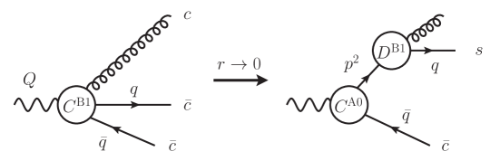
Figure 3: Representation of the B1 matching coefficient factorization in the soft-quark limit given in (19).

The matching coefficient $D^{\rm B1}(p^{2})$ is a universal function that will appear in different processes involving soft quark emission. The DL resummation of $D^{\rm B1}(p^{2})$ has been derived in [7]. It comprises the all-order $(C_{A}-C_{F})^{n}$ colour coefficient that appears to be characteristic in soft quark emissions [15, 6, 7]. The identical coefficient also enters the $ggH$ amplitude with a bottom-quark loop and was computed recently at two-loops [16]. The $D^{\rm B1}(p^{2})$ coefficient and its evolution equation can be obtained from the corresponding B1 operator coefficients and anomalous dimension [17, 18] by taking the limit $r\to 0$. The extraction of the anomalous dimension resembles to the derivation of the asymptotic kernel for the QED light-meson light-cone distribution amplitude [19], see also [10]. For the derivation and results, we refer to appendix A of [1]. When the gluon is replaced by a photon, the abelian version of $D^{\rm B1}(p^{2})$ corresponds to the jet function in the LP factorization of $B\to\gamma\ell\nu$ [20], and in the NLP endpoint factorization of the $H\to\gamma\gamma$ amplitude [10]. In the abelian case, the evolution up to two loops was inferred from renormalization-group consistency of the $B\to\gamma\ell\nu$ observable [21]. The one-loop evolution kernel of the jet function has also been obtained by direct computation in [22].

4.2 Endpoint factorization consistency conditions

As motivated in section 2 and confirmed explicitly above at $\mathcal{O}(\alpha_{s})$, we expect the integrands of the A- and B-type terms to have the same asymptotic limits to all orders, which is a prerequisite for endpoint factorization. Concretely, the limit of the anti-collinear momentum $n_{-}\cdot p_{\bar{c}}=rQ,r^{\prime}Q\to 0$ in the B-type term should match the limit $n_{-}\cdot k=\omega,\omega^{\prime}\to\infty$ of the corresponding soft momentum component in the A-type term. The above picture is formalized by the two refactorization conditions [1]:

(I) $$\hskip 14.22636pt\mathcal{J}_{c}\left(p^{2},\omega,\omega^{\prime}\right)=\mathcal{J}_{c}^{(g)}(p^{2})\,\displaystyle\frac{D^{\rm B1}(\omega Q)}{\omega}\frac{{D^{\rm B1}}^{*}(\omega^{\prime}Q)}{\omega^{\prime}}+\mathcal{O}\!\left(\frac{1}{\omega^{(\prime)}}\right)\,,$$ (20)

and

(II) $$\hskip-42.67912ptQ\,\widetilde{\mathcal{J}}^{(\bar{q})}_{\bar{c}}(s_{R})\,\widetilde{S}_{\rm NLP}\left(s_{R},s_{L},\omega,\omega^{\prime}\right)\Big{|}_{\omega^{(\prime)}\to\infty}$$ (21)

$$\hskip 71.13188pt\displaystyle=\widetilde{\mathcal{J}}^{q\bar{q}(8)}_{\bar{c}}\left(s_{R},r,r^{\prime}\right)\widetilde{S}^{(g)}(s_{R},s_{L})\Big{|}_{r^{(\prime)}=\omega^{(\prime)}/Q\to 0}\,.$$

For large $\omega$, the soft quark field in $S_{\rm NLP}$ turns anti-collinear, $\bar{q}_{s}Y_{n_{-}}\to\bar{\chi}_{\bar{c}}$, so it moves from $S_{\rm NLP}$ to $\mathcal{J}^{q\bar{q}(8)}_{\bar{c}}$. Removing $\bar{q}_{s}Y_{n_{-}}$ from $S_{\rm NLP}$ leaves the LP soft function $S^{(g)}$, and adding it as $\bar{\chi}_{\bar{c}}$ to $\mathcal{J}^{(\bar{q})}_{\bar{c}}$ changes the anti-quark jet function into $\mathcal{J}^{q\bar{q}(8)}_{\bar{c}}$. In total, this results in $S_{\rm NLP}\mathcal{J}^{(\bar{q})}_{\bar{c}}\to S^{(g)}\mathcal{J}^{q\bar{q}(8)}_{\bar{c}}$, which is relation (II). At the same time, the quark fields in the A-type collinear function become highly off-shell, which removes them from $\mathcal{J}_{c}(p^{2},\omega,\omega^{\prime})$. This leaves behind only the collinear gluon, so $C^{\rm A0}$ turns into $C^{\rm B1}$. Therefore, $|C^{\rm A0}|^{2}\mathcal{J}_{c}\to|C^{\rm B1}|^{2}\mathcal{J}_{c}^{(g)}$, which is relation (I).

4.3 Endpoint factorization formula

We can now state the endpoint-finite factorization formula. To do so concisely, we use the double-bracket notation introduced in [9] to denote the asymptotic behaviours of the various functions. In functions of $\omega,\omega^{\prime}$, rescale $\omega\to\kappa\omega$, $\omega^{\prime}\to\kappa\omega^{\prime}$ and take $\kappa\to\infty$. Then

$$\llbracket S_{\rm NLP}\left(l_{+},l_{-},\omega,\omega^{\prime}\right)\rrbracket\equiv S_{\rm NLP}\left(l_{+},l_{-},\omega,\omega^{\prime}\right)|_{\mathcal{O}(\kappa^{0})},$$ (22)

$$\llbracket\mathcal{J}_{c}(p^{2},\omega,\omega^{\prime})\rrbracket\equiv\mathcal{J}_{c}(p^{2},\omega,\omega^{\prime})|_{\mathcal{O}(\kappa^{-2})}\,.$$ (23)

The right-hand side of the above equation equals the right-hand side of the consistency relation (I). Similarly, in functions of $r,r^{\prime}$, rescale $r\to r\kappa$, $r^{\prime}\to r^{\prime}\kappa$ and take $\kappa\to 0$, or the corresponding rescaling is applied to $\bar{r}$, $\bar{r}^{\prime}$. Which of the two is meant, will be indicated by the subscript 0 or 1 on the double bracket. Then $\llbracket C^{\rm B1}_{1}(Q^{2},r)\rrbracket_{0}\equiv C^{\rm B1}_{1}(Q^{2},r)|_{\mathcal{O}(\kappa^{-1})}\,$, and $\llbracket C^{\rm B1}_{2}(Q^{2},r)\rrbracket_{1}\equiv C^{\rm B1}_{2}(Q^{2},r)|_{\mathcal{O}(\kappa^{-1})}\,$, while $\llbracket C^{\rm B1}_{1}(Q^{2},r)\rrbracket_{1}=\llbracket C^{\rm B1}_{2}(Q^{2},r)\rrbracket_{0}=0$. To implement the rearrangement of endpoint-singular terms we introduce the scaleless integral

$$\frac{2C_{F}}{Q}\,f(\epsilon)\,|C^{\rm A0}|^{2}\widetilde{\mathcal{J}}^{(\bar{q})}_{\bar{c}}\widetilde{\mathcal{J}}_{c}^{(g)}\int_{0}^{\infty}d\omega d\omega^{\prime}\,\frac{D^{\rm B1}(\omega Q)}{\omega}\frac{D^{\rm B1*}(\omega^{\prime}Q)}{\omega^{\prime}}\left\llbracket\widetilde{S}_{\rm NLP}(s_{R},s_{L},\omega,\omega^{\prime})\right\rrbracket,$$ (24)

which vanishes in $d$-dimensions. We split this integral in two terms $I_{1,2}$, $I_{1}+I_{2}=0$, with $I_{1}$ being defined by $\omega$ or $\omega^{\prime}$ smaller than a parameter $\Lambda$ and $I_{2}$ the complement region, as shown on the left-hand side of figure 4. In the complement region $\omega,\omega^{\prime}>\Lambda$, and the double-bracket asymptotic behaviour can be used for functions of $\omega,\omega^{\prime}$ in the A-type term. The endpoint rearrangement consists of subtracting $I_{1}$ from the B-type term and $I_{2}$ from the A-type term. The subtracted expressions are now separately endpoint-finite, but depend on $\Lambda$ which cancels exactly between the two terms as long as we do not make further approximations.

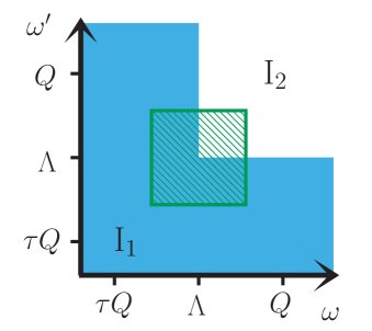
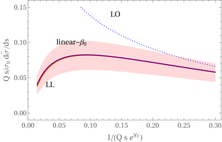
Figure 4: On the left we show the split of (24) into $I_{1}+I_{2}$ according to the correspondingly indicated regions in the $\omega-\omega^{\prime}$ plane as described in the text below (24). In the overlap region in green the asymptotic behaviour of the A- and B-type term must agree. On the right, we display the Laplace-space LL gluon thrust distribution. Variation of the initial scales as described in the text yields the light-red band.

Starting with the A-type contribution,subtracting from it the complement region $I_{2}$ of the integral (24), and using the endpoint factorization conditions results in

$$\frac{1}{\sigma_{0}}\frac{\widetilde{d\sigma}}{ds_{R}ds_{L}}|_{\rm A-type}\! = \frac{2C_{F}}{Q}|C^{\rm A0}|^{2}\,\widetilde{\mathcal{J}}_{\bar{c}}^{(\bar{q})}\,\int_{0}^{\infty}d\omega d\omega^{\prime}\,\bigg{\{}\,\widetilde{\mathcal{J}}_{c}(s_{L},\omega,\omega^{\prime})\,\widetilde{S}_{\rm NLP}(s_{R},s_{L},\omega,\omega^{\prime})$$ (25)

$$-\,\theta(\omega-\Lambda)\theta(\omega^{\prime}-\Lambda)\,\llbracket\widetilde{\mathcal{J}}_{c}(s_{L},\omega,\omega^{\prime})\rrbracket\llbracket\widetilde{S}_{\rm NLP}(s_{R},s_{L},\omega,\omega^{\prime})\rrbracket$$

$$+\;\,\widetilde{\!\!\widehat{\mathcal{J}}}_{\!c}(s_{L},\omega,\omega^{\prime})\,\,\widetilde{\!\widehat{S}}_{\rm NLP}(s_{R},s_{L},\omega,\omega^{\prime})\,\bigg{\}}\,,\quad$$

where we set $f(\epsilon)=1$ as $\epsilon\to 0$. The remaining part $I_{1}$ of the integral (24) is now combined with $i=i^{\prime}=1$ part of the B-type term, and after using refactorization conditions we have

$$\frac{1}{\sigma_{0}}\frac{\widetilde{d\sigma}}{ds_{R}ds_{L}}|_{\scriptsize{\begin{array}[]{l}$\rm B--type$\\[-2.84544pt] $i=i'=1$\end{array}}}\! = \frac{2C_{F}}{Q^{2}}\widetilde{\mathcal{J}}_{c}^{(g)}\,\widetilde{S}^{(g)}(s_{R},s_{L})\,\int_{0}^{\infty}drdr^{\prime}\,\bigg{[}$$ (29)

$$\theta(1-r)\theta(1-r^{\prime})C^{\rm B1*}_{1}(r^{\prime})C^{\rm B1}_{1}(r)\,\widetilde{\mathcal{J}}_{\bar{c}}^{q\bar{q}(8)}(s_{R},r,r^{\prime})$$

$$-\big{[}1-\theta(r-\Lambda/Q)\theta(r^{\prime}-\Lambda/Q)\big{]}\,\llbracket C^{\rm B1*}_{1}(r^{\prime})\rrbracket_{0}\,\llbracket C^{\rm B1}_{1}(r)\rrbracket_{0}\,\llbracket\widetilde{\mathcal{J}}_{\bar{c}}^{q\bar{q}(8)}(s_{R},r,r^{\prime})\rrbracket_{0}\bigg{]}\,.$$

The $i=i^{\prime}=2$ term with the anti-quark becoming soft takes a similar form and is explicitly provided in [1].

5 Resummation

Solving of the necessary RG equations for the objects appearing in the above factorization formulas is discussed in detail in sections 5.1 and 5.2 of [1]. The final result for the leading-logarithmic accurate resummed expression after all the individual pieces combined together reads in Laplace space:

$$\frac{1}{\sigma_{0}}\frac{\widetilde{d\sigma}}{ds_{R}ds_{L}}|_{\rm LL} = 2\cdot\frac{2C_{F}}{Qs_{R}}\frac{\alpha_{s}(\mu_{c})}{4\pi}\,\,\exp\left[4C_{F}S\left(\mu_{h},\mu_{\bar{c}}\right)+4C_{A}S\left(\mu_{s},\mu_{c}\right)\right]\times\left(\frac{Q^{2}}{\mu_{h}^{2}}\right)^{\!-2C_{F}A\left(\mu_{h},\mu_{\bar{c}}\right)}$$ (30)

$$\times\left(\frac{1}{s_{L}s_{R}e^{2\gamma_{E}}\mu_{s}^{2}}\right)^{\!-2C_{A}A\left(\mu_{s},\mu_{c}\right)}\int_{\sigma}^{Q}\frac{d\omega}{\omega}\,\left(\frac{\omega}{s_{R}e^{\gamma_{E}}\mu_{s\Lambda}^{2}}\right)^{\!-2\left(C_{F}-C_{A}\right)A\left(\mu_{s\Lambda},\mu_{h\Lambda}\right)}$$

$$\times\exp\left[4\left(C_{F}-C_{A}\right)S\left(\mu_{s\Lambda},\mu_{h\Lambda}\right)\right]\,\left(s_{R}e^{\gamma_{E}}Q\right)^{2C_{F}A\left(\mu_{h\Lambda},\mu_{\bar{c}}\right)+2C_{A}A\left(\mu_{c},\mu_{h\Lambda}\right)}\,,$$

with the functions $S\left(\nu,\mu\right)$ and $A_{\gamma_{i}}\left(\nu,\mu\right)$ defined as in [23]. We note that $\mu^{2}_{h\Lambda}\sim\omega Q$ and $\mu^{2}_{s\Lambda}\sim\omega/s_{R}$ are $\omega$-dependent scales that appear inside the integrand for reasons explained in [1]. The importance of next-to-leading logarithms can be studied by varying the various matching scales around the values adopted in (30). We vary the three pairs of scales $(\mu_{h},\mu_{h\Lambda})$, $(\mu_{c},\mu_{\bar{c}})$, $(\mu_{s},\mu_{s\Lambda})$ by a factor of $1/2$ and 2 around their default scales. Taking the minimum and maximum values to compute the scale variation. We show this for the normalized Laplace-space distribution $\frac{Qs}{\sigma_{0}}\frac{\widetilde{d\sigma}}{ds}$ in the right-hand panel of figure 4 as the light-red band around the red curve (LL) that represents (30). For comparison, the tree-level (LO) and linear-$\beta_{0}$ truncation of the LL expression are displayed. The sizeable scale variation in the figure emphasizes the need for NLL resummation. The endpoint-rearranged factorization formula presented in this work provides the starting point for this systematic improvement.

6 Conclusion

In this work, we summarized the derivation of a novel endpoint factorization relation for the NLP gluon-thrust distribution in the two-jet region, as achieved in [1]. This off-diagonal contribution contains a gluon-initiated jet recoiling against a quark-antiquark pair, which involves subleading-power cross-section level soft and jet functions. The framework shares many similarities with the rearrangement employed for the resummation of the $H\to\gamma\gamma$ bottom-loop amplitude [9, 10] and allows for the first time to systematically remove endpoint divergences in the convolution integrals of SCET_I factorization theorems, opening the path to NLP resummation for collider observables with soft quark emission. Employing the subtraction of endpoint divergences with the aid of operatorial factorization conditions, we managed to reshuffle the factorization theorem such that the individual terms are free from endpoint divergences and can be written in terms of renormalized hard, (anti) collinear, and soft functions in four dimensions. At this point, standard RG techniques can be applied to obtain the resummed integrands. In [1], we derived the anomalous dimensions of the NLP jet and soft functions using RG consistency and endpoint factorization relations. We also calculated the one-loop anomalous dimension for the hard matching coefficients, which enabled us to perform the first resummation of the endpoint-divergent SCET_I observable at the LL accuracy using exclusively RG methods. We verified that our results can recover the earlier results at DL accuracy [6, 7] and we evaluated the numerical impact of the LL corrections. Our main result for gluon-thrust is (30), which provides an expression for the two-hemisphere invariant mass distribution in Laplace space. The next step in further exploration of NLP resummation is the extension of the present work and related soft-quark emission processes to NLL accuracy, which requires the calculation of renormalization kernels for the NLP soft and jet functions at order $\mathcal{O}(\alpha_{s})$, and application of the methods presented here to address endpoint divergent issues appearing in diagonal channels of relevant processes.

Acknowledgements

This work has been supported by the Excellence Cluster ORIGINS funded by the Deutsche Forschungsgemeinschaft (DFG, German Research Foundation) under Germany’s Excellence Strategy –EXC-2094 –390783311. S.J. is supported by the UK Science and Technology Facilities Council under grant ST/T001011/1. R.S. is supported by the United States Department of Energy under Grant Contract DE-SC0012704. L.V. is funded by Fellini Fellowship for Innovation at INFN, and by the European Union’s Horizon 2020 research programme under the Marie Skłodowska-Curie Cofund Action, grant agreement no. 754496. J.W. is funded by the National Natural Science Foundation of China (No. 12005117) and the Taishan Scholar Foundation of Shandong province (tsqn201909011).

References

- [1] M. Beneke, M. Garny, S. Jaskiewicz, J. Strohm, R. Szafron, L. Vernazza et al., Next-to-leading power endpoint factorization and resummation for off-diagonal “gluon” thrust, JHEP 07 (2022) 144, [2205.04479].
- [2] S. Catani, G. Turnock, B. R. Webber and L. Trentadue, Thrust distribution in e+ e- annihilation, Phys. Lett. B 263 (1991) 491–497.
- [3] S. Catani, L. Trentadue, G. Turnock and B. R. Webber, Resummation of large logarithms in e+ e- event shape distributions, Nucl. Phys. B 407 (1993) 3–42.
- [4] T. Becher and M. D. Schwartz, A precise determination of from LEP thrust data using effective field theory, JHEP 07 (2008) 034, [0803.0342].
- [5] M. Beneke, A. Broggio, S. Jaskiewicz and L. Vernazza, Threshold factorization of the Drell-Yan process at next-to-leading power, JHEP 07 (2020) 078, [1912.01585].
- [6] I. Moult, I. W. Stewart, G. Vita and H. X. Zhu, The Soft Quark Sudakov, JHEP 05 (2020) 089, [1910.14038].
- [7] M. Beneke, M. Garny, S. Jaskiewicz, R. Szafron, L. Vernazza and J. Wang, Large-x resummation of off-diagonal deep-inelastic parton scattering from d-dimensional refactorization, JHEP 10 (2020) 196, [2008.04943].
- [8] I. Moult, I. W. Stewart and G. Vita, Subleading Power Factorization with Radiative Functions, JHEP 11 (2019) 153, [1905.07411].
- [9] Z. L. Liu and M. Neubert, Factorization at subleading power and endpoint-divergent convolutions in decay, JHEP 04 (2020) 033, [1912.08818].
- [10] Z. L. Liu, B. Mecaj, M. Neubert and X. Wang, Factorization at subleading power and endpoint divergences in decay. Part II. Renormalization and scale evolution, JHEP 01 (2021) 077, [2009.06779].
- [11] M. Beneke, A. P. Chapovsky, M. Diehl and T. Feldmann, Soft collinear effective theory and heavy to light currents beyond leading power, Nucl. Phys. B643 (2002) 431–476, [hep-ph/0206152].
- [12] C. W. Bauer, D. Pirjol and I. W. Stewart, Soft collinear factorization in effective field theory, Phys. Rev. D65 (2002) 054022, [hep-ph/0109045].
- [13] I. Moult, L. Rothen, I. W. Stewart, F. J. Tackmann and H. X. Zhu, Subleading Power Corrections for N-Jettiness Subtractions, Phys. Rev. D95 (2017) 074023, [1612.00450].
- [14] M. Beneke and L. Vernazza, decays revisited, Nucl. Phys. B 811 (2009) 155–181, [0810.3575].
- [15] A. Vogt, Leading logarithmic large-x resummation of off-diagonal splitting functions and coefficient functions, Phys. Lett. B 691 (2010) 77–81, [1005.1606].
- [16] Z. L. Liu, M. Neubert, M. Schnubel and X. Wang, Radiative quark jet function with an external gluon, JHEP 02 (2022) 075, [2112.00018].
- [17] M. Beneke, M. Garny, R. Szafron and J. Wang, Anomalous dimension of subleading-power N-jet operators, JHEP 03 (2018) 001, [1712.04416].
- [18] M. Beneke, M. Garny, R. Szafron and J. Wang, Anomalous dimension of subleading-power -jet operators. Part II, JHEP 11 (2018) 112, [1808.04742].
- [19] M. Beneke, P. Böer, J.-N. Toelstede and K. K. Vos, Light-cone distribution amplitudes of light mesons with QED effects, JHEP 11 (2021) 059, [2108.05589].
- [20] S. W. Bosch, R. J. Hill, B. O. Lange and M. Neubert, Factorization and Sudakov resummation in leptonic radiative B decay, Phys. Rev. D 67 (2003) 094014, [hep-ph/0301123].
- [21] Z. L. Liu and M. Neubert, Two-Loop Radiative Jet Function for Exclusive -Meson and Higgs Decays, JHEP 06 (2020) 060, [2003.03393].
- [22] G. T. Bodwin, J.-H. Ee, J. Lee and X.-P. Wang, Renormalization of the radiative jet function, Phys. Rev. D 104 (2021) 116025, [2107.07941].
- [23] M. Neubert, Renormalization-group improved calculation of the branching ratio, Eur. Phys. J. C 40 (2005) 165–186, [hep-ph/0408179].