Relevant Analytic Spontaneous Magnetization
Relation for the Face-Centered-Cubic Ising Lattice

Abstract

The relevant approximate spontaneous magnetization relations for the simple-cubic and body-centered-cubic Ising lattices have recently been obtained analytically by a novel approach that conflates the Callen–Suzuki identity with a heuristic odd-spin correlation magnetization relation. By exploiting this approach, we study an approximate analytic spontaneous magnetization expression for the face-centered-cubic Ising lattice. We report that the results of the analytic relation obtained in this work are nearly consistent with those derived from the Monte Carlo simulation.

I Introduction

Concerning the phase transition theory [1], the Ising model [2] is one of the most studied spin systems that exhibits a phase transition at a nonzero finite temperature when the dimension $d\geq 2$, resulting in spontaneous magnetization from spontaneously broken discrete $\mathbb{Z}_{2}$ global symmetry [3]. The Hamiltonian of the Ising model is given by

$$\mathcal{H}=-J\sum_{\langle i,j\rangle}\sigma_{i}\sigma_{j},$$

where, $J$ is the coupling strength, $\sum_{\langle i,j\rangle}$ indicates the summation over nearest neighbors, $\sigma_{i}$ may take values $\pm 1$, and its symmetry time-reversal $\mathbb{Z}_{2}$ originates in that leaves it invariant under the $\sigma_{i}\rightarrow-\sigma_{i}{}$ transformation. The exact solutions of one-dimensional and two-dimensional (2D) rectangular lattice Ising models were performed by, respectively, Ising [2] and Onsager [4]. The former has no spontaneous magnetization since it does not undergo a phase transition at a nonzero finite temperature due to its dimensionality. The latter, besides having an exact solution, has an exact spontaneous magnetization relation obtained by Yang [5]. Though this was previously obtained by Onsager and Kaufman [6], they never published their derivation. After these pioneering contributions by Onsager and Yang for the 2D rectangular lattice Ising model, the exact solutions and exact spontaneous magnetization relations for the other various 2D lattices, e.g., honeycomb, triangular, etc., were also obtained [7, 8, 9, 10, 11, 12, 13, 14, 15, 16].

The three-dimensional (3D) Ising model, although subjected to a number of notable attempted solutions [17, 18, 19, 20, 21, 22, 23] and recent advances [24, 25, 26, 27], remains a big mystery as to whether or not it can be solved exactly [28]. The lack of exact treatments, as in the case of the 3D Ising model, necessitates the development of approximate methods and concepts in order to explore and detect the emergence properties and critical values in a tractable manner while studying phase transition theory [29]. These methods and concepts vary from renormalization group theory [30, 31, 32, 33], series expansions [34, 35], field-theoretic [36], conformal bootstrap [37, 38], Monte Carlo (MC) simulations [39, 40, 41, 42, 43, 44, 45, 46, 47, 48, 49, 50], and recently developed machine-learning-aided techniques [51, 52, 53, 54, 55, 56]. For a further discussion on the exact results and approximate methods, we recommend seeing Refs. [57, 58, 59, 60, 61, 62, 63]. The Ising model, with its existing exact treatment literature [2, 4, 5, 7, 8, 9, 10, 11, 12, 13, 14, 15, 16, 64, 65, 66, 67, 68, 69, 70, 71, 72, 73], even if it falls in a limited region, plays a central role in the testing ground for the new methods and techniques and finds interdisciplinary applications in the fields where complexity and intractability emerge, such as economics [74, 75, 76], biology [77, 78], sociology [79], neuroscience [80, 81], and deep learning [82, 83], etc.

Considering the spontaneous magnetization of the 3D Ising model, a most recent approach in the context of effective field theory [58] given by Kaya [84, 85, 86] has successively led to the derivation of relevant approximate analytic spontaneous magnetization relations for the simple-cubic (SC) and body-centered-cubic Ising lattices. This has been achieved by proposing a heuristic odd-spin correlation magnetization (OSCM) relation by means of associating it to the Callen–Suzuki [69, 87, 88] identity. In order for the OSCM (heuristic Kaya relation) to apply in this approach, it requires a form of expanded Callen–Suzuki identity in terms of odd-spin correlations. Briefly, the heuristic OSCM relation implements the idea given in the following statement: the odd-spin correlations in the vicinity of the critical point decay as power-law with the same critical exponent of the spontaneous magnetization but with different amplitudes. This was concluded previously for three-point correlations thereby the exact relations performed by Baxter [89] on the triangular Ising lattice. Such behavior, however, is not very well known for the higher-order odd-correlations when we consider they have relatively restricted literature [90], unlike three-point correlations [91, 92, 93, 94, 95, 96, 97, 98, 99]. Nevertheless, the validity of this approach has been verified [86, 84] on the 2D Ising lattices, e.g., honeycomb, square, and triangular, where there are exact expressions for the spontaneous magnetization [5, 14, 15] to be compared. For the SC Ising lattice, it has also been reported that the results derived from this approach [84] are in agreement with those of an empirical relation obtained by Talapov and Blöte [100] decades ago. It should also be noted that the critical values needed within this approach, i.e., critical temperature and critical exponent, are made supplementary use of the present results in the literature. As a complementary work, in the present paper, we shall utilize this approach to obtain a relevant approximate analytic spontaneous magnetization expression for a far more complex crystal structure, the face-centered-cubic (FCC) Ising lattice, and perform an MC simulation to compare the results of this analytic relation with those of the MC simulation.

It has been pointed out [101, 24, 25, 26, 27] that in 3D lattices, in addition to the contribution from the local spin alignment, there is one more type of contribution to the physical properties (including spontaneous magnetization). The latter is due to the nontrivial topological contributions, i.e., the long-range entanglements among the spins. For a further discussion, see Ref. [24]. We would like to acknowledge that the present method in this paper does not study such nontrivial topological contributions to spontaneous magnetization.

II Methods and Results

II.1 Expansion of the Callen–Suzuki Identity

Let us begin by writing down the Callen–Suzuki identity as

$$\left\langle\sigma_{i}\right\rangle=\left\langle\tanh{\left(K\sum_{j}^{q}\sigma_{j}\right)}\right\rangle,$$ (1)

where, $K=J/(k_{B}T)$, here $T$ and $k_{B}$ correspond, respectively, to the temperature and the Boltzmann’s constant, $\left\langle\cdots\right\rangle$ indicates the ensemble average, $\sigma_{j}$’s are the neighboring spins while $\sigma_{i}$ is the central spin, and $q$ denotes the number of nearest neighbors, which is equal to 12 for the FCC lattice. The $\tanh{}$ term given above can be expanded as

$$\tanh{\left(K\sum_{j}^{12}\sigma_{j}\right)} =A\sum_{(12)}\sigma_{j}+B\sum_{(220)}\sigma_{j_{1}}\sigma_{j_{2}}\sigma_{j_{3}}+C\sum_{(792)}\sigma_{j_{1}}\sigma_{j_{2}}\sigma_{j_{3}}\sigma_{j_{4}}\sigma_{j_{5}}+D\sum_{(792)}\sigma_{j_{1}}\sigma_{j_{2}}\sigma_{j_{3}}\sigma_{j_{4}}\sigma_{j_{5}}\sigma_{j_{6}}\sigma_{j_{7}}$$

$$\qquad+E\sum_{(220)}\sigma_{j_{1}}\sigma_{j_{2}}\sigma_{j_{3}}\sigma_{j_{4}}\sigma_{j_{5}}\sigma_{j_{6}}\sigma_{j_{7}}\sigma_{j_{8}}\sigma_{j_{9}}+F\sum_{(12)}\sigma_{j_{1}}\sigma_{j_{2}}\sigma_{j_{3}}\sigma_{j_{4}}\sigma_{j_{5}}\sigma_{j_{6}}\sigma_{j_{7}}\sigma_{j_{8}}\sigma_{j_{9}}\sigma_{j_{10}}\sigma_{j_{11}},$$ (2)

where, summations for each odd-spin terms run over the combinations of a given configuration $\sigma_{j_{1}},\sigma_{j_{2}},\ldots,\sigma_{j_{12}}$ of the neighboring spins. One can prove the expansion as follows: feeding a fully pointing down configuration, $\{-1,-1,\ldots,-1\}$, into the $\tanh$ term demonstrates that no terms with an even number of spins are allowed to occur in the right-hand-side because $\tanh$ is an odd function. Moreover, the permutation symmetry does not allow for more than six different coefficients. These unknown coefficients $A,B,\ldots,F$, can be determined self-consistently by considering all $2^{12}$ configurations of the neighboring spins. Substituting all configurations into Equation (II.1) results in only six unique equations

$$\tanh\left(2K\right) =2A-10B+20C-20D+10E-2F,$$

$$\tanh\left(4K\right) =4A-12B+8C+8D-12E+4F,$$

$$\tanh\left(6K\right) =6A+2B-36C+36D-2E+6F,$$

$$\tanh\left(8K\right) =8A+40B-48C-48D+40E+8F,$$

$$\tanh\left(10K\right) =10A+110B+132C-132D-100E-10F,$$

$$\tanh\left(12K\right) =12A+220B+792C+792D+220E+12F,$$

through this set of equations, the coefficients can be obtained straightforwardly as follows

$$A(K) =\frac{1}{2048}\big{[}132\tanh{\left(2K\right)}+165\tanh{\left(4K\right)}+110\tanh{\left(6K\right)}+44\tanh{\left(8K\right)}+10\tanh{\left(10K\right)}+\tanh{\left(12K\right)}\big{]},$$

$$B(K) =\frac{1}{2048}\big{[}-36\tanh{\left(2K\right)}-27\tanh{\left(4K\right)}+2\tanh{\left(6K\right)}+12\tanh{\left(8K\right)}+6\tanh{\left(10K\right)}+\tanh{\left(12K\right)}\big{]},$$

$$C(K) =\frac{1}{2048}\big{[}20\tanh{\left(2K\right)}+5\tanh{\left(4K\right)}-10\tanh{\left(6K\right)}-4\tanh{\left(8K\right)}+2\tanh{\left(10K\right)}+\tanh{\left(12K\right)}\big{]},$$

$$D(K) =\frac{1}{2048}\big{[}-20\tanh{\left(2K\right)}+5\tanh{\left(4K\right)}+10\tanh{\left(6K\right)}-4\tanh{\left(8K\right)}-2\tanh{\left(10K\right)}+\tanh{\left(12K\right)}\big{]},$$

$$E(K) =\frac{1}{2048}\big{[}36\tanh{\left(2K\right)}-27\tanh{\left(4K\right)}-2\tanh{\left(6K\right)}+12\tanh{\left(8K\right)}-6\tanh{\left(10K\right)}+\tanh{\left(12K\right)}\big{]},$$

$$F(K) =\frac{1}{2048}\big{[}-132\tanh{\left(2K\right)}+165\tanh{\left(4K\right)}-110\tanh{\left(6K\right)}+44\tanh{\left(8K\right)}-10\tanh{\left(10K\right)}+\tanh{\left(12K\right)}\big{]}.$$

Substituting Equation (II.1) into Equation (1) and then taking averages over them yields a form of expanded Callen–Suzuki identity in terms of odd-spin correlations as given in the following

$$\left\langle\sigma\right\rangle =12A(K)\left\langle\sigma\right\rangle+220B(K)\left\langle\sigma_{j_{1}}\sigma_{j_{2}}\sigma_{j_{3}}\right\rangle+792C(K)\left\langle\sigma_{j_{1}}\sigma_{j_{2}}\sigma_{j_{3}}\sigma_{j_{4}}\sigma_{j_{5}}\right\rangle+792D(K)\left\langle\sigma_{j_{1}}\sigma_{j_{2}}\sigma_{j_{3}}\sigma_{j_{4}}\sigma_{j_{5}}\sigma_{j_{6}}\sigma_{j_{7}}\right\rangle$$

$$\quad+220E(K)\left\langle\sigma_{j_{1}}\sigma_{j_{2}}\sigma_{j_{3}}\sigma_{j_{4}}\sigma_{j_{5}}\sigma_{j_{6}}\sigma_{j_{7}}\sigma_{j_{8}}\sigma_{j_{9}}\right\rangle+12F(K)\left\langle\sigma_{j_{1}}\sigma_{j_{2}}\sigma_{j_{3}}\sigma_{j_{4}}\sigma_{j_{5}}\sigma_{j_{6}}\sigma_{j_{7}}\sigma_{j_{8}}\sigma_{j_{9}}\sigma_{j_{10}}\sigma_{j_{11}}\right\rangle,$$ (3)

where we have used $\left\langle\sigma_{i}\right\rangle=\left\langle\sigma_{j}\right\rangle\equiv\left\langle\sigma\right\rangle$. The combinations of the pairwise distances of the neighboring spins on the lattice are different from one another, and the correlation amplitude between two spins on the different lattice locations is the function of this pairwise distance [90]. It will be, therefore, more convenient to group these correlations with respect to the sum of the pairwise distances of the neighboring spins on the lattice for each odd-spin correlation as

$$220\left\langle\sigma_{j_{1}}\sigma_{j_{2}}\sigma_{j_{3}}\right\rangle =8\left\langle\sigma_{1}\sigma_{5}\sigma_{8}\right\rangle+24\left\langle\sigma_{1}\sigma_{2}\sigma_{5}\right\rangle+24\left\langle\sigma_{1}\sigma_{5}\sigma_{12}\right\rangle+48\left\langle\sigma_{1}\sigma_{2}\sigma_{12}\right\rangle+24\left\langle\sigma_{1}\sigma_{5}\sigma_{10}\right\rangle+48\left\langle\sigma_{1}\sigma_{3}\sigma_{12}\right\rangle+12\left\langle\sigma_{1}\sigma_{2}\sigma_{3}\right\rangle$$

$$\quad+24\left\langle\sigma_{1}\sigma_{2}\sigma_{11}\right\rangle+8\left\langle\sigma_{1}\sigma_{6}\sigma_{11}\right\rangle,$$

$$792\left\langle\sigma_{j_{1}}\sigma_{j_{2}}\cdots\sigma_{j_{5}}\right\rangle =36\left\langle\sigma_{1}\sigma_{2}\sigma_{5}\sigma_{9}\sigma_{12}\right\rangle+48\left\langle\sigma_{1}\sigma_{2}\sigma_{5}\sigma_{8}\sigma_{12}\right\rangle+24\left\langle\sigma_{1}\sigma_{2}\sigma_{4}\sigma_{9}\sigma_{12}\right\rangle+48\left\langle\sigma_{1}\sigma_{2}\sigma_{5}\sigma_{6}\sigma_{12}\right\rangle+24\left\langle\sigma_{1}\sigma_{2}\sigma_{4}\sigma_{8}\sigma_{12}\right\rangle$$

$$\quad+24\left\langle\sigma_{1}\sigma_{2}\sigma_{5}\sigma_{10}\sigma_{12}\right\rangle+72\left\langle\sigma_{1}\sigma_{2}\sigma_{3}\sigma_{9}\sigma_{12}\right\rangle+96\left\langle\sigma_{1}\sigma_{2}\sigma_{5}\sigma_{11}\sigma_{12}\right\rangle+48\left\langle\sigma_{1}\sigma_{2}\sigma_{3}\sigma_{10}\sigma_{12}\right\rangle+48\left\langle\sigma_{1}\sigma_{4}\sigma_{5}\sigma_{6}\sigma_{9}\right\rangle$$

$$\quad+72\left\langle\sigma_{1}\sigma_{2}\sigma_{3}\sigma_{11}\sigma_{12}\right\rangle+48\left\langle\sigma_{1}\sigma_{3}\sigma_{5}\sigma_{11}\sigma_{12}\right\rangle+48\left\langle\sigma_{1}\sigma_{3}\sigma_{6}\sigma_{8}\sigma_{12}\right\rangle+48\left\langle\sigma_{1}\sigma_{2}\sigma_{6}\sigma_{11}\sigma_{12}\right\rangle+24\left\langle\sigma_{1}\sigma_{2}\sigma_{3}\sigma_{4}\sigma_{5}\right\rangle$$

$$\quad+24\left\langle\sigma_{1}\sigma_{2}\sigma_{3}\sigma_{8}\sigma_{12}\right\rangle+36\left\langle\sigma_{1}\sigma_{2}\sigma_{7}\sigma_{10}\sigma_{12}\right\rangle+24\left\langle\sigma_{1}\sigma_{2}\sigma_{3}\sigma_{7}\sigma_{12}\right\rangle,$$

$$792\left\langle\sigma_{j_{1}}\sigma_{j_{2}}\cdots\sigma_{j_{7}}\right\rangle =36\left\langle\sigma_{1}\sigma_{2}\sigma_{3}\sigma_{9}\sigma_{10}\sigma_{11}\sigma_{12}\right\rangle+48\left\langle\sigma_{1}\sigma_{2}\sigma_{3}\sigma_{5}\sigma_{9}\sigma_{10}\sigma_{12}\right\rangle+24\left\langle\sigma_{1}\sigma_{2}\sigma_{3}\sigma_{6}\sigma_{9}\sigma_{10}\sigma_{12}\right\rangle+48\left\langle\sigma_{1}\sigma_{2}\sigma_{4}\sigma_{5}\sigma_{8}\sigma_{11}\sigma_{12}\right\rangle$$

$$\quad+24\left\langle\sigma_{1}\sigma_{2}\sigma_{3}\sigma_{4}\sigma_{9}\sigma_{10}\sigma_{12}\right\rangle+24\left\langle\sigma_{1}\sigma_{2}\sigma_{3}\sigma_{5}\sigma_{8}\sigma_{9}\sigma_{12}\right\rangle+72\left\langle\sigma_{1}\sigma_{2}\sigma_{3}\sigma_{5}\sigma_{6}\sigma_{8}\sigma_{12}\right\rangle+96\left\langle\sigma_{1}\sigma_{2}\sigma_{3}\sigma_{5}\sigma_{10}\sigma_{11}\sigma_{12}\right\rangle$$

$$\quad+48\left\langle\sigma_{1}\sigma_{2}\sigma_{5}\sigma_{7}\sigma_{9}\sigma_{11}\sigma_{12}\right\rangle+48\left\langle\sigma_{1}\sigma_{2}\sigma_{3}\sigma_{7}\sigma_{10}\sigma_{11}\sigma_{12}\right\rangle+72\left\langle\sigma_{1}\sigma_{2}\sigma_{3}\sigma_{5}\sigma_{7}\sigma_{9}\sigma_{12}\right\rangle+48\left\langle\sigma_{1}\sigma_{2}\sigma_{3}\sigma_{6}\sigma_{7}\sigma_{9}\sigma_{12}\right\rangle$$

$$\quad+48\left\langle\sigma_{1}\sigma_{2}\sigma_{3}\sigma_{4}\sigma_{5}\sigma_{11}\sigma_{12}\right\rangle+48\left\langle\sigma_{1}\sigma_{2}\sigma_{3}\sigma_{5}\sigma_{8}\sigma_{11}\sigma_{12}\right\rangle+24\left\langle\sigma_{1}\sigma_{2}\sigma_{3}\sigma_{4}\sigma_{8}\sigma_{10}\sigma_{12}\right\rangle+24\left\langle\sigma_{1}\sigma_{2}\sigma_{3}\sigma_{4}\sigma_{5}\sigma_{7}\sigma_{12}\right\rangle$$

$$\quad+36\left\langle\sigma_{1}\sigma_{2}\sigma_{3}\sigma_{7}\sigma_{8}\sigma_{11}\sigma_{12}\right\rangle+24\left\langle\sigma_{1}\sigma_{2}\sigma_{3}\sigma_{5}\sigma_{7}\sigma_{11}\sigma_{12}\right\rangle,$$

$$220\left\langle\sigma_{j_{1}}\sigma_{j_{2}}\cdots\sigma_{j_{9}}\right\rangle =8\left\langle\sigma_{1}\sigma_{2}\sigma_{3}\sigma_{5}\sigma_{6}\sigma_{9}\sigma_{10}\sigma_{11}\sigma_{12}\right\rangle+24\left\langle\sigma_{1}\sigma_{2}\sigma_{3}\sigma_{4}\sigma_{5}\sigma_{6}\sigma_{7}\sigma_{8}\sigma_{12}\right\rangle+24\left\langle\sigma_{1}\sigma_{2}\sigma_{3}\sigma_{5}\sigma_{8}\sigma_{9}\sigma_{10}\sigma_{11}\sigma_{12}\right\rangle$$

$$\quad+48\left\langle\sigma_{1}\sigma_{2}\sigma_{3}\sigma_{4}\sigma_{5}\sigma_{6}\sigma_{8}\sigma_{9}\sigma_{12}\right\rangle+24\left\langle\sigma_{1}\sigma_{2}\sigma_{3}\sigma_{5}\sigma_{6}\sigma_{7}\sigma_{8}\sigma_{11}\sigma_{12}\right\rangle+48\left\langle\sigma_{1}\sigma_{3}\sigma_{5}\sigma_{6}\sigma_{7}\sigma_{9}\sigma_{10}\sigma_{11}\sigma_{12}\right\rangle$$

$$\quad+12\left\langle\sigma_{1}\sigma_{2}\sigma_{3}\sigma_{4}\sigma_{5}\sigma_{7}\sigma_{9}\sigma_{11}\sigma_{12}\right\rangle+24\left\langle\sigma_{1}\sigma_{2}\sigma_{3}\sigma_{4}\sigma_{5}\sigma_{6}\sigma_{7}\sigma_{10}\sigma_{12}\right\rangle+8\left\langle\sigma_{1}\sigma_{2}\sigma_{3}\sigma_{5}\sigma_{7}\sigma_{8}\sigma_{10}\sigma_{11}\sigma_{12}\right\rangle,$$

where, the correlations specified by the neighboring spins on the lattice, as indicated in Fig. 1, represent the entire group to which they belong, and the correlations here have been chosen arbitrarily from the group in which they are included. On the other hand, the last term in Equation (II.1) has not been grouped since the sum of the pairwise distances of all the combinations on the lattice are equal to each other.

For the proof, the derivation, and further discussions for the Callen–Suzuki identity and its odd-spin correlation expansion for the six neighboring spins (e.g., SC lattice), similar to what we detailed in this paper, see Refs. [65, 21, 58, 88, 90].

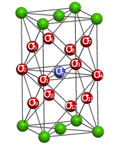
Figure 1: (Color Online) A diagram of FCC lattice. $\sigma_{1},\sigma_{2},\ldots,\sigma_{12}$ (red spins) denote the neighboring spins whereas $\sigma_{0}$ (blue spin) denotes the central spin.

II.2 Derivation of the Analytic Relation for the Spontaneous Magnetization

We now proceed by introducing the heuristic Kaya relation as given in Refs. [86, 84, 85] in the form

$$\left\langle\sigma_{j_{1}}\sigma_{j_{2}}\ldots\sigma_{j_{k}}\right\rangle=\lambda_{k,r}\left\langle\sigma\right\rangle+\left(1-\lambda_{k,r}\right)\left\langle\sigma\right\rangle^{\frac{1+\beta}{\beta}},$$ (4)

in which $k$ on the subscript is an odd number that refers to the order of the odd-correlations, $r$ labels the groups, $\beta$ denotes the critical exponent, and $\lambda_{k,r}$ may take $0\leq\lambda_{k,r}\leq 1$ values by definition [86, 84, 85]. Applying Equation (4) to all the grouped correlations and then substituting these expressions into Equation (II.1) leads to

$$\left\langle\sigma\right\rangle =\left\langle\sigma\right\rangle\big{(}12A+B\mathcal{C}_{3}+C\mathcal{C}_{5}+D\mathcal{C}_{7}+E\mathcal{C}_{9}+F\mathcal{C}_{11}\big{)}$$

$$\quad+\left\langle\sigma\right\rangle^{\frac{1+\beta}{\beta}}\big{(}220B+792C+792D+220E+12F$$

$$\qquad\qquad\qquad-B\mathcal{C}_{3}-C\mathcal{C}_{5}-D\mathcal{C}_{7}-E\mathcal{C}_{9}-F\mathcal{C}_{11}\big{)},$$

where,

$$\mathcal{C}_{3} \equiv 8\lambda_{3,1}+24\lambda_{3,2}+24\lambda_{3,3}+48\lambda_{3,4}+24\lambda_{3,5}+48\lambda_{3,6}+12\lambda_{3,7}+24\lambda_{3,8}+8\lambda_{3,9},$$

$$\mathcal{C}_{5} \equiv 36\lambda_{5,1}+48\lambda_{5,2}+24\lambda_{5,3}+48\lambda_{5,4}+24\lambda_{5,5}+24\lambda_{5,6}+72\lambda_{5,7}+96\lambda_{5,8}+48\lambda_{5,9}+48\lambda_{5,10}$$

$$\quad+72\lambda_{5,11}+48\lambda_{5,12}+48\lambda_{5,13}+48\lambda_{5,14}+24\lambda_{5,15}+24\lambda_{5,16}+36\lambda_{5,17}+24\lambda_{5,18},$$

$$\mathcal{C}_{7} \equiv 36\lambda_{7,1}+48\lambda_{7,2}+24\lambda_{7,3}+48\lambda_{7,4}+24\lambda_{7,5}+24\lambda_{7,6}+72\lambda_{7,7}+96\lambda_{7,8}+48\lambda_{7,9}+48\lambda_{7,10}$$

$$\quad+72\lambda_{7,11}+48\lambda_{7,12}+48\lambda_{7,13}+48\lambda_{7,14}+24\lambda_{7,15}+24\lambda_{7,16}+36\lambda_{7,17}+24\lambda_{7,18},$$

$$\mathcal{C}_{9} \equiv 8\lambda_{9,1}+24\lambda_{9,2}+24\lambda_{9,3}+48\lambda_{9,4}+24\lambda_{9,5}+48\lambda_{9,6}+12\lambda_{9,7}+24\lambda_{9,8}+8\lambda_{9,9},$$

$$\mathcal{C}_{11} \equiv 12\lambda_{11,1}.$$

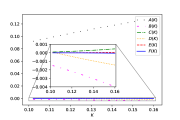
Figure 2: (Color Online) The plots of $A(K)$, $B(K)$, $C(K)$, $D(K)$, $E(K)$, and $F(K)$ versus $K$. The lines loosely-dotted (black), loosely-dash-dotted (magenta), dash-dotted (green), dotted (orange), dashed (red), and solid (blue) correspond to $A(K)$, $B(K)$, $C(K)$, $D(K)$, $E(K)$, and $F(K)$, respectively. The inset zooms in the selected region in the figure.

Now, let us cancel $\left\langle\sigma\right\rangle$ terms in Equation (II.2), then, it turns out to be

$$1 =\big{(}12A+B\mathcal{C}_{3}+C\mathcal{C}_{5}+D\mathcal{C}_{7}+E\mathcal{C}_{9}+F\mathcal{C}_{11}\big{)}$$

$$\quad+\left\langle\sigma\right\rangle^{\frac{1}{\beta}}\big{(}220B+792C+792D+220E+12F$$

$$\qquad\qquad\quad-B\mathcal{C}_{3}-C\mathcal{C}_{5}-D\mathcal{C}_{7}-E\mathcal{C}_{9}-F\mathcal{C}_{11}\big{)}.$$

As these $\lambda_{k,r}$s are unknown, we restrict ourselves to adopting an approximation at this stage. As can be seen in Fig. 2, $E(K)$ and $F(K)$ give almost no contribution. Thus, we can omit the $\mathcal{C}_{9}$ and $\mathcal{C}_{11}$ terms since they are multiplied by $E(K)$ and $F(K)$, respectively. The remaining terms $\mathcal{C}_{3}$, $\mathcal{C}_{5}$, and $\mathcal{C}_{7}$ can be assumed to be nearly equal to each other. Hence, we summarize the approximation we shall adopt as follows

$$\mathcal{C}_{3}\simeq\mathcal{C}_{5}\simeq\mathcal{C}_{7},$$ (7a)

$$E(K),F(K)\approx 0.$$ (7b)

Within this approximation, we reduce the number of unknown parameters to only one, which is $\mathcal{C}_{3}$, and then calculate this single unknown parameter by using the behavior of the spontaneous magnetization in the vicinity of the critical point $K_{c}$ as given by

$$\left\langle\sigma\right\rangle=\begin{cases}\neq 0,&K>K_{c},\\ 0,&K\leq K_{c}.\end{cases}$$

Once the approximation procedure given in Equations (7a) and (7b) is applied, Equation (II.2) then becomes

$$1 =12A+\mathcal{C}_{3}\big{(}B(K)+C(K)+D(K)\big{)}$$

$$\quad+\left\langle\sigma\right\rangle^{\frac{1}{\beta}}\bigg{[}220B(K)+792C(K)+792D(K)-\mathcal{C}_{3}\big{(}B(K)+C(K)+D(K)\big{)}\bigg{]}.$$ (8)

To determine the $\mathcal{C}_{3}$ from Equation (8) with the aid of the aforementioned behavior of spontaneous magnetization, we need the $K_{c}$ value. For which we take $K_{c}=0.1270707\pm 0.0000002$ as predicted in Ref. [48], which is the most recent result in the literature. There are also some other predictions in Refs. [47, 46], nevertheless, all of them are consistent with one another within the respective error bars. From now on, we abbreviate the terms that contain uncertainty by using shorthand notation, e.g., $K_{c}=0.1270707(2)$, for simplicity. Now, since the last term $\left\langle\sigma\right\rangle^{\frac{1}{\beta}}$ in Equation (8) vanishes at the critical point $K_{c}$, we thus calculate $\mathcal{C}_{3}$ by

$$\left(\frac{1-12A(K)}{B(K)+C(K)+D(K)}\right)\bigg{|}_{K=K_{c}}=\mathcal{C}_{3},$$ (9)

and we obtain $\mathcal{C}_{3}=74.3922(9)$. Now, substituting the $\mathcal{C}_{3}$ term into Equation (8) and then rearranging it leads to spontaneous magnetization

$$\left\langle\sigma\right\rangle=\left[\frac{1-12A(K)-\mathcal{C}_{3}\big{(}B(K)+C(K)+D(K)\big{)}}{220B(K)+792C(K)+792D(K)-\mathcal{C}_{3}\big{(}B(K)+C(K)+D(K)\big{)}}\right]^{\beta}.$$ (10)

The analytic relation given in Equation (10) has been plotted in Fig. 3, where we have taken the critical exponent $\beta=0.32630(22)$ [49] for the 3D Ising universality class.

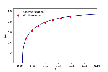
Figure 3: (Color Online) The plot of $K$ versus $\langle\sigma\rangle$. The solid (blue) line and the filled points (red) correspond to Equation (10) and the MC data, respectively. The figure also includes error bars; however, they are invisible because they are smaller than the marker points.

II.3 Spontaneous Magnetization through MC Simulation

To obtain the spontaneous magnetization of the FCC Ising lattice by a different and reliable method, we have also performed an MC simulation by employing the Wolff [42] cluster MC algorithm. It is one of the most efficient algorithms for the 3D Ising model [102] because it does not suffer from the critical slowing down in the vicinity of the critical point.

In this process, at each $K$ point, we ran the simulation on a relatively larger $256\times 256\times 256$ lattice with periodic boundary conditions to avoid the finite size and edge effects. We then collected data at every correlation time interval after running a sufficient number (2000) of thermalization time steps. To minimize statistical errors, we set the correlation time interval $\tau$ to 50. We thus have calculated the spontaneous magnetization using the relation

$$\left\langle\sigma\right\rangle=\left\langle\left\lvert\frac{1}{N}\sum_{i}\sigma_{i}\right\rvert\right\rangle,$$

where, $N$ is the number of spins on the lattice, $\lvert\cdots\rvert$ indicates the absolute value, and averages run over the thermal states (or configurations). The results have been displayed in Fig. 3. The error bars were also constructed using Jackknife analysis [39]; however, they are invisible as they are smaller than the marker points.

III Discussion and Conclusions

In this work, we have studied spontaneous magnetization for the FCC Ising lattice and have obtained an expression as given in Equation (10). To show the relevance of the analytic relation, we have also performed an MC simulation. The results of both the MC simulation and Equation (10) have been plotted in Fig. 3, where the solid line (blue) and filled marker points (red) correspond to the results of the analytic relation and those derived from the MC simulation, respectively. As can be seen in Fig. 3, there is a minute difference between the centers of the filled points and the solid line. Since the resolution of the figure does not allow for the viewing of error bars, there is no information as to whether the solid line passes through the error bars of the filled points or not. Consequently, we do not have strong evidence to support the claim that there is an inconsistency between these results. We, therefore, simply interpret that these results are nearly consistent with each other due to the fact that the solid line intersects with the filled points. On the other hand, if there is a deviation, this could either arise from the approximation we adopted in the derivation of the analytic relation as given in Equations (7a) and (7b) or from the inherent drawbacks of the MC simulations such as finite size effects. Nevertheless, in the MC simulation, we set the lattice size to $L=256$, which is a highly sufficient lattice size to minimize this effect as reported in Ref. [100]. Therefore, as further work, one may clarify these points that we stressed out by calculating the $\mathcal{C}_{3},\mathcal{C}_{5},\ldots,\mathcal{C}_{11}$ values empirically through an MC simulation. This could be simply realized by recalling Equation (4) in the form

$$\lambda_{k,r}=\frac{\left\langle\sigma_{j_{1}}\sigma_{j_{2}}\ldots\sigma_{j_{k}}\right\rangle-\left\langle\sigma\right\rangle^{\frac{1+\beta}{\beta}}}{\left\langle\sigma\right\rangle-\left\langle\sigma\right\rangle^{\frac{1+\beta}{\beta}}}.$$

As $K$ is approached to the $K_{c}^{+}$, the $\left\langle\sigma\right\rangle^{\frac{1+\beta}{\beta}}$ term above goes to zero more rapidly than the other terms. Thus, near the critical point, the $\lambda_{k,r}$ simply becomes amplitude ratio, as shown in the following

$$\lambda_{k,r}\simeq\frac{\left\langle\sigma_{j_{1}}\sigma_{j_{2}}\ldots\sigma_{j_{k}}\right\rangle}{\left\langle\sigma\right\rangle}.$$

Once $\lambda_{k,r}$’s terms have been calculated over odd-spin correlation and spontaneous magnetization at the critical point $K_{c}$, it would then be quite straightforward to derive an analytic relation similar to the one performed in this paper.

Considering the fact that the spontaneous magnetization expression of the FCC lattice Ising model is a long-standing open problem, we would like to emphasize that the relation we have obtained herein is quite relevant and remarkable regardless of whether it requires a better approximation at the stage of its derivation.

Funding

This research received no external funding.

Data Availability

The datasets generated during and/or analysed during the current study are available from the author on reasonable request.

Acknowledgments

The author would like to thank Yaşar Seher for their support in drawing the FCC diagram.

Conflict of Iinterest

The author declares no conflict of interest.

References

- Stanley [1971] H. Stanley, Introduction to Phase Transitions and Critical Phenomena, International series of monographs on physics (Oxford University Press, New York, 1971).
- Ising [1925] E. Ising, Contribution to the theory of ferromagnetism, Z. Phys. 31, 253 (1925).
- Smits et al. [2021] J. Smits, H. T. C. Stoof, and P. van der Straten, Spontaneous breaking of a discrete time-translation symmetry, Phys. Rev. A 104, 023318 (2021).
- Onsager [1944] L. Onsager, Crystal statistics. I. a two-dimensional model with an order-disorder transition, Phys. Rev. 65, 117 (1944).
- Yang [1952] C. N. Yang, The spontaneous magnetization of a two-dimensional Ising model, Phys. Rev. 85, 808 (1952).
- Baxter [2012] R. J. Baxter, Onsager and Kaufman’s calculation of the spontaneous magnetization of the Ising model: II, J. Stat. Phys. 149, 1164 (2012).
- Houtappel [1950] R. Houtappel, Order-disorder in hexagonal lattices, Physica 16, 425 (1950).
- Husimi and Syôzi [1950] K. Husimi and I. Syôzi, The statistics of honeycomb and triangular lattice. I, Prog. Theor. Phys. 5, 177 (1950).
- Syozi [1950] I. Syozi, The statistics of honeycomb and triangular lattice. II, Prog. Theor. Phys. 5, 341 (1950).
- Newell [1950] G. F. Newell, Crystal statistics of a two-dimensional triangular Ising lattice, Phys. Rev. 79, 876 (1950).
- Temperley [1950] H. Temperley, Statistical mechanics of the two-dimensional assembly, Proc. R. Soc. Lond. A Math. Phys. Sci. 202, 202 (1950).
- Wannier [1950] G. H. Wannier, Antiferromagnetism. the triangular Ising net, Phys. Rev. 79, 357 (1950).
- Potts [1955] R. B. Potts, Combinatorial solution of the triangular Ising lattice, Proc. Phys. Soc. A 68, 145 (1955).
- Naya [1954] S. Naya, On the Spontaneous Magnetizations of Honeycomb and Kagomé Ising Lattices, Prog. Theor. Phys. 11, 53 (1954).
- Potts [1952] R. B. Potts, Spontaneous magnetization of a triangular Ising lattice, Phys. Rev. 88, 352 (1952).
- Lin and Ma [1983] K. Y. Lin and W. J. Ma, Two-dimensional Ising model on a ruby lattice, J. Phys. A Math. Gen. 16, 3895 (1983).
- Zhang [2007] Z.-D. Zhang, Conjectures on the exact solution of three-dimensional (3d) simple orthorhombic Ising lattices, Phil. Mag. 87, 5309 (2007).
- Wu et al. [2008] F. Wu, B. McCoy, M. Fisher, and L. Chayes, Comment on a recent conjectured solution of the three-dimensional Ising model, Phil. Mag. 88, 3093 (2008).
- Perk [2009] J. H. Perk, Comment on ‘conjectures on exact solution of three-dimensional (3d) simple orthorhombic Ising lattices’, Phil. Mag. 89, 761 (2009).
- Zhang [2009] Z. Zhang, Response to the comment on ‘conjectures on exact solution of three-dimensional (3d) simple orthorhombic Ising lattices’, Phil. Mag. 89, 765 (2009).
- Perk [2012] J. H. H. Perk, Erroneous solution of three-dimensional (3d) simple orthorhombic Ising lattices, Bull. Société Sci. Lettres LÓDZ 62, 45 (2012), arXiv:1209.0731 [cond-mat] .
- Zhang [2013] Z.-D. Zhang, Mathematical structure of the three-dimensional (3d) Ising model, Chin. Phys. B 22, 030513 (2013).
- Perk [2013] J. H. H. Perk, Comment on ‘mathematical structure of the three-dimensional (3d) Ising model’, Chin. Phys. B 22, 080508 (2013).
- Zhang et al. [2019] Z. Zhang, O. Suzuki, and N. H. March, Clifford algebra approach of 3d Ising model, Adv. Appl. Clifford Algebras 29, 12 (2019).
- Suzuki and Zhang [2021] O. Suzuki and Z. Zhang, A method of Riemann–Hilbert problem for Zhang’s conjecture 1 in a ferromagnetic 3d Ising model: Trivialization of topological structure, Mathematics 9, 776 (2021).
- Zhang and Suzuki [2021] Z. Zhang and O. Suzuki, A method of the Riemann–Hilbert problem for Zhang’s conjecture 2 in a ferromagnetic 3d Ising model: Topological phases, Mathematics 9, 2936 (2021).
- Zhang [2022] Z. Zhang, Topological quantum statistical mechanics and topological quantum field theories, Symmetry 14, 323 (2022).
- Viswanathan et al. [2022] G. M. Viswanathan, M. A. G. Portillo, E. P. Raposo, and M. G. E. da Luz, What does it take to solve the 3d ising model? minimal necessary conditions for a valid solution, Entropy 24, 1665 (2022).
- Domb [1960] C. Domb, On the theory of cooperative phenomena in crystals, Adv. Phys. 9, 245 (1960).
- Wilson [1971a] K. G. Wilson, Renormalization group and critical phenomena. i. renormalization group and the Kadanoff scaling picture, Phys. Rev. B 4, 3174 (1971a).
- Wilson [1971b] K. G. Wilson, Renormalization group and critical phenomena. ii. phase-space cell analysis of critical behavior, Phys. Rev. B 4, 3184 (1971b).
- Wilson [1983] K. G. Wilson, The renormalization group and critical phenomena, Rev. Mod. Phys. 55, 583 (1983).
- Goldenfeld [1992] N. Goldenfeld, Lectures on phase transitions and the renormalization group (CRC Press, Boca Raton, 1992).
- Butera and Comi [2002] P. Butera and M. Comi, Critical universality and hyperscaling revisited for Ising models of general spin using extended high-temperature series, Phys. Rev. B 65, 144431 (2002).
- Salman and Adler [1998] Z. Salman and J. Adler, High and low temperature series estimates for the critical temperature of the 3d Ising model, Int. J. Mod. Phys. C 9, 195 (1998).
- Jasch and Kleinert [2001] F. Jasch and H. Kleinert, Fast-convergent resummation algorithm and critical exponents of -theory in three dimensions, J. Math. Phys. 42, 52 (2001).
- El-Showk et al. [2012] S. El-Showk, M. F. Paulos, D. Poland, S. Rychkov, D. Simmons-Duffin, and A. Vichi, Solving the 3d Ising model with the conformal bootstrap, Phys. Rev. D 86, 025022 (2012).
- El-Showk et al. [2014] S. El-Showk, M. F. Paulos, D. Poland, S. Rychkov, D. Simmons-Duffin, and A. Vichi, Solving the 3d Ising model with the conformal bootstrap II. -minimization and precise critical exponents, J. Stat. Phys. 157, 869 (2014).
- Landau and Binder [2014] D. P. Landau and K. Binder, A Guide to Monte Carlo Simulations in Statistical Physics, 4th ed. (Cambridge University Press, Cambridge, 2014).
- Metropolis et al. [1953] N. Metropolis, A. W. Rosenbluth, M. N. Rosenbluth, A. H. Teller, and E. Teller, Equation of state calculations by fast computing machines, J. Chem. Phys. 21, 1087 (1953).
- Swendsen and Wang [1987] R. H. Swendsen and J.-S. Wang, Nonuniversal critical dynamics in monte carlo simulations, Phys. Rev. Lett. 58, 86 (1987).
- Wolff [1989] U. Wolff, Collective monte carlo updating for spin systems, Phys. Rev. Lett. 62, 361 (1989).
- Hasenbusch [2001] M. Hasenbusch, Monte carlo studies of the three-dimensional Ising model in equilibrium, Int. J. Mod. Phys. C 12, 911 (2001).
- Blöte et al. [1996] H. W. J. Blöte, J. R. Heringa, A. Hoogland, E. W. Meyer, and T. S. Smit, Monte carlo renormalization of the 3d Ising model: Analyticity and convergence, Phys. Rev. Lett. 76, 2613 (1996).
- Gupta and Tamayo [1996] R. Gupta and P. Tamayo, Critical exponents of the 3-d Ising model, Int. J. Mod. Phys. C 07, 305 (1996).
- Murase and Ito [2007] Y. Murase and N. Ito, Dynamic critical exponents of three-dimensional Ising models and two-dimensional three-states Potts models, J. Phys. Soc. Japan 77, 014002 (2007).
- Lundow et al. [2009] P. H. Lundow, K. Markström, and A. Rosengren, The Ising model for the bcc, fcc and diamond lattices: A comparison, Phil. Mag. 89, 2009 (2009).
- Yu [2015] U. Yu, Critical temperature of the Ising ferromagnet on the fcc, hcp, and dhcp lattices, Phys. A: Stat. Mech. Appl. 419, 75 (2015).
- Ferrenberg et al. [2018] A. M. Ferrenberg, J. Xu, and D. P. Landau, Pushing the limits of monte carlo simulations for the three-dimensional Ising model, Phys. Rev. E 97, 043301 (2018).
- Netz and Berker [1991] R. R. Netz and A. N. Berker, Monte carlo mean-field theory and frustrated systems in two and three dimensions, Phys. Rev. Lett. 66, 377 (1991).
- Wang [2016] L. Wang, Discovering phase transitions with unsupervised learning, Phys. Rev. B 94, 195105 (2016).
- Torlai and Melko [2016] G. Torlai and R. G. Melko, Learning thermodynamics with Boltzmann machines, Phys. Rev. B 94, 165134 (2016).
- Carrasquilla and Melko [2017] J. Carrasquilla and R. G. Melko, Machine learning phases of matter, Nat. Phys. 13, 431 (2017).
- Hu et al. [2017] W. Hu, R. R. P. Singh, and R. T. Scalettar, Discovering phases, phase transitions, and crossovers through unsupervised machine learning: A critical examination, Phys. Rev. E 95, 062122 (2017).
- Chung and Kao [2021] J.-H. Chung and Y.-J. Kao, Neural monte carlo renormalization group, Phys. Rev. Res. 3, 023230 (2021).
- Carleo et al. [2019] G. Carleo, I. Cirac, K. Cranmer, L. Daudet, M. Schuld, N. Tishby, L. Vogt-Maranto, and L. Zdeborová, Machine learning and the physical sciences, Rev. Mod. Phys. 91, 045002 (2019).
- Hu [2014] C.-K. Hu, Historical review on analytic, monte carlo, and renormalization group approaches to critical phenomena of some lattice models, Chin. J. Phys. 52, 1 (2014).
- Strecka and Jaščur [2015] J. Strecka and M. Jaščur, A brief account of the Ising and Ising-like models: Mean-field, effective-field and exact results, Acta Phys. Slovaca 65, 235 (2015), arXiv:1511.03031 [cond-mat] .
- McCoy [2009] B. McCoy, Advanced Statistical Mechanics, International series of monographs on physics (Oxford University Press, New York, 2009).
- Kardar [2007] M. Kardar, Statistical Physics of Fields (Cambridge University Press, Cambridge, 2007).
- McCoy and Wu [2014] B. M. McCoy and T. T. Wu, The two-dimensional Ising Model (Courier Corporation, New York, 2014).
- Baxter [1982] R. J. Baxter, Exactly Solved Models in Statistical Mechanics (Academic Press, London, 1982).
- Pelissetto and Vicari [2002] A. Pelissetto and E. Vicari, Critical phenomena and renormalization-group theory, Phys. Rep. 368, 549 (2002).
- Kramers and Wannier [1941] H. A. Kramers and G. H. Wannier, Statistics of the two-dimensional ferromagnet. part I, Phys. Rev. 60, 252 (1941).
- Fisher [1959] M. E. Fisher, Transformations of Ising models, Phys. Rev. 113, 969 (1959).
- Kaufman [1949] B. Kaufman, Crystal statistics. II. partition function evaluated by spinor analysis, Phys. Rev. 76, 1232 (1949).
- Kaufman and Onsager [1949] B. Kaufman and L. Onsager, Crystal statistics. III. short-range order in a binary Ising lattice, Phys. Rev. 76, 1244 (1949).
- Perk [1980] J. Perk, Quadratic identities for Ising model correlations, Phys. Lett. A 79, 3 (1980).
- Callen [1963] H. Callen, A note on Green functions and the Ising model, Phys. Lett. 4, 161 (1963).
- Yang [1988] C. N. Yang, Journey through statistical mechanics, Int. J. Mod. Phys. B 02, 1325 (1988).
- Kac and Ward [1952] M. Kac and J. C. Ward, A combinatorial solution of the two-dimensional Ising model, Phys. Rev. 88, 1332 (1952).
- Hurst and Green [1960] C. A. Hurst and H. S. Green, New solution of the Ising problem for a rectangular lattice, J. Chem. Phys. 33, 1059 (1960).
- Montroll et al. [1963] E. W. Montroll, R. B. Potts, and J. C. Ward, Correlations and spontaneous magnetization of the two‐dimensional Ising model, J. Math. Phys. 4, 308 (1963).
- Bornholdt and Wagner [2002] S. Bornholdt and F. Wagner, Stability of money: phase transitions in an Ising economy, Phys. A: Stat. Mech. Appl. 316, 453 (2002).
- Sornette and Zhou [2006] D. Sornette and W.-X. Zhou, Importance of positive feedbacks and overconfidence in a self-fulfilling Ising model of financial markets, Phys. A: Stat. Mech. Appl. 370, 704 (2006).
- Stauffer [2008] D. Stauffer, Social applications of two-dimensional Ising models, Am. J. Phys. 76, 470 (2008).
- Weber and Buceta [2016] M. Weber and J. Buceta, The cellular Ising model: a framework for phase transitions in multicellular environments, J. R. Soc. Interface 13, 20151092 (2016).
- Matsuda [1981] H. Matsuda, The Ising Model for Population Biology, Prog. Theor. Phys. 66, 1078 (1981).
- Castellano et al. [2009] C. Castellano, S. Fortunato, and V. Loreto, Statistical physics of social dynamics, Rev. Mod. Phys. 81, 591 (2009).
- Schneidman et al. [2006] E. Schneidman, M. J. Berry, R. Segev, and W. Bialek, Weak pairwise correlations imply strongly correlated network states in a neural population, Nature 440, 1007 (2006).
- Amit [1989] D. J. Amit, Modeling Brain Function: The World of Attractor Neural Networks (Cambridge University Press, Cambridge, 1989).
- Decelle and Furtlehner [2021] A. Decelle and C. Furtlehner, Restricted Boltzmann machine: Recent advances and mean-field theory, Chin. Phys. B 30, 040202 (2021).
- Engel and Van den Broeck [2001] A. Engel and C. Van den Broeck, Statistical Mechanics of Learning (Cambridge University Press, Cambridge, 2001).
- Kaya [2022a] T. Kaya, Relevant spontaneous magnetization relations for the triangular and the cubic lattice Ising model, Chin. J. Phys. 77, 2676 (2022a).
- Kaya [2022b] T. Kaya, Analytic average magnetization expression for the body-centered cubic Ising lattice, Eur. Phys. J. Plus 137, 1130 (2022b).
- Kaya [2022c] T. Kaya, Relevant alternative analytic average magnetization calculation method for the square and the honeycomb Ising lattices, Chin. J. Phys. 77, 747 (2022c).
- Suzuki [1965] M. Suzuki, Generalized exact formula for the correlations of the Ising model and other classical systems, Phys. Lett. 19, 267 (1965).
- Suzuki [2002] M. Suzuki, Correlation identities and application, Int. J. Mod. Phys. B 16, 1749 (2002).
- Baxter [1975] R. Baxter, Triplet order parameter of the triangular Ising model, J. Phys. A Math. Gen. 8, 1797 (1975).
- Barry et al. [1982] J. Barry, C. Múnera, and T. Tanaka, Exact solutions for Ising model odd-number correlations on the honeycomb and triangular lattices, Phys. A: Stat. Mech. Appl. 113, 367 (1982).
- Pink [1968] D. A. Pink, Three-site correlation functions of the two-dimensional Ising model, Can. J. Phys. 46, 2399 (1968).
- Enting [1977] I. G. Enting, Triplet order parameters in triangular and honeycomb Ising models, J. Phys. A Math. Gen. 10, 1737 (1977).
- Barber [1976] M. N. Barber, On the nature of the critical point in the three-spin triangular Ising model, J. Phys. A Math. Gen. 9, L171 (1976).
- Wood and Griffiths [1976] D. W. Wood and H. P. Griffiths, Triplet order parameters for three-dimensional Ising models, J. Phys. A Math. Gen. 9, 407 (1976).
- Taggart [1982] G. B. Taggart, Effective field model for Ising ferromagnets: Influence of triplet correlations, J. Appl. Phys. 53, 1907 (1982).
- Baxter and Choy [1989] R. J. Baxter and T. C. Choy, Local three-spin correlations in the free-fermion and planar Ising models, Proc. R. Soc. Lond. A Math. Phys. Sci. 423, 279 (1989).
- Kaya [2020] T. Kaya, Exact three spin correlation function relations for the square and the honeycomb Ising lattices, Chin. J. Phys. 66, 415 (2020).
- Lin [1989] K. Y. Lin, Three-spin correlation of the Ising model on the generalized checkerboard lattice, J. Stat. Phys. 56, 631 (1989).
- Lin and Chen [1990] K. Y. Lin and B. H. Chen, Three-spin correlation of the Ising model on a Kagome lattice, Int. J. Mod. Phys. B 04, 123 (1990).
- Talapov and Blöte [1996] A. L. Talapov and H. W. J. Blöte, The magnetization of the 3d Ising model, J. Phys. A Math. Gen. 29, 5727 (1996).
- Newell and Montroll [1953] G. F. Newell and E. W. Montroll, On the theory of the Ising model of ferromagnetism, Rev. Mod. Phys. 25, 159 (1953).
- Binder and Luijten [2001] K. Binder and E. Luijten, Monte carlo tests of renormalization-group predictions for critical phenomena in Ising models, Phys. Rep. 344, 179 (2001).