Continuum Thermodynamics of the Phase Transformation of Thermoelastic Fluids

Abstract.

This study uses continuum thermodynamics of pure thermoelastic fluids to examine their phase transformation. To examine phase transformation kinetics, a special emphasis is placed on the jump condition for the axiom of entropy inequality, thereby recovering the conventional result that stable phase equilibrium coincides with continuity of temperature, pressure, and free enthalpy across the phase boundary. Moreover, this jump condition leads to the formulation of a constitutive relation for the phase transformation mass flux, $-\left[\left[\frac{1}{T}\mathbf{q}\right]\right]\cdot\mathbf{n}^{\Gamma}/\left[\left[s\right]\right]$, where $\left[\left[\frac{1}{T}\mathbf{q}\right]\right]\cdot\mathbf{n}^{\Gamma}$ is the jump in entropy flux normal to, and across the phase interface $\Gamma$, and $\left[\left[s\right]\right]$ is the corresponding jump in entropy. This relation implies that phase transformations must be accompanied by a jump in temperature across the phase boundary. Encouraging agreement is found between this formula and limited available experimental data. Further evidence is needed to conclusively validate this proposed constitutive model. This continuum framework is well suited for implementation in a computational framework, such as the finite element method.

1. Introduction

The primary objective of this study is to formulate phase transformation kinetics of pure thermoelastic fluids under general ‘non-equilibrium’ conditions. We present a complete approach for formulating constitutive models for real gases and liquids, of the type used to populate thermodynamic tables, using virial expansions. Our approach employs the specific free energy as the main function of state that needs to be characterized to completely describe the properties of a thermoelastic fluid. By adopting an arbitrary reference pressure and reference temperature, we obtain relatively simple expressions for the specific free energy of real liquids and gases.

We place a special emphasis on understanding jump conditions across interfaces, especially those involving a jump in temperature in the absence or presence of a phase transformation. We show that the concepts of specific enthalpy and specific free enthalpy emerge naturally from those jump conditions, albeit using gauge instead of absolute pressure. To examine phase transformations, we adopt the framework of reactive mixture theory [36, 14, 8, 1] to model a phase transformation as a reaction, and specialize it to conditions prevailing across the phase boundary. We verify that our approach reproduces the classical result that pressure, temperature and specific free enthalpy are continuous across the phase boundary at phase equilibrium, though we also find that continuity of temperature is only sufficient, not necessary to satisfy the entropy inequality under these conditions.

Finally, we propose a constitutive relation for the reactive (e.g., evaporative) mass flux across a phase boundary which satisfies the entropy inequality jump that regulates the feasibility of interfacial processes. We find that this reactive mass flux for phase transformation can only occur in the presence of a non-zero temperature jump and a non-zero average heat flux across the phase boundary. By also satisfying the mass, momentum and energy jumps, this constitutive relation produces a unique solution for the jump in temperature during a phase transformation. This novel constitutive relation is grounded entirely in the framework of continuum mechanics, without appeal to the kinetic theory of gases or statistical rate theory.

A purely continuum-based formulation was adopted here because it represents a fundamental framework employed by engineers for analyzing thermofluid processes. We recognize that the axiomatic presentation of conservation laws for mass, momentum and energy, and the entropy inequality, are not always favored in other fields of the physical sciences. However, it is not our purpose here to present a universal, or molecular, or statistical foundation for thermodynamics of phase transformations. Instead, for those investigators who favor the continuum approach, our goal with this study is to fill a missing element of this framework, namely by providing a method to formulate and constrain a constitutive model for the evaporation or condensation rates in a phase transformation.

2. Kinematics and Notation Convention

We describe the motion of a thermoelastic fluid using the standard approach in continuum mechanics (for example, see Chapter 2 of [22]). Let $\mathbf{X}$ denote the position of a material particle in the reference configuration and let $\mathbf{x}$ represent the spatial position of this particle at the current time $t$. The motion of the particle is given by the function $\boldsymbol{\chi}$, such that $\mathbf{x}=\boldsymbol{\chi}\left(\mathbf{X},t\right)$. Any function $f$ associated with the material (such as its temperature $T$, velocity $\mathbf{v}$, mass density $\rho$, etc.) may be expressed mathematically in the material frame as $\check{f}\left(\mathbf{X},t\right)$ and in the spatial frame as $\tilde{f}\left(\mathbf{x},t\right)$, such that $f=\check{f}\left(\mathbf{X},t\right)=\tilde{f}\left(\mathbf{x},t\right)$. This identity remains valid component-wise when $f$ is a tensor of any order, as long as $\mathbf{x}$ and $\mathbf{X}$ are expressed in the same basis. The material time derivative of $f$ is denoted by $\dot{f}$. It may be evaluated in either frame as

$$\dot{f}=\frac{\partial\check{f}}{\partial t}=\frac{\partial\tilde{f}}{\partial t}+\operatorname{grad}\tilde{f}\cdot\mathbf{v}\,,$$ (2.1)

where $\operatorname{grad}\tilde{f}=\partial\tilde{f}/\partial\mathbf{x}$ and $\mathbf{v}=\partial\boldsymbol{\chi}/\partial t$ is the material’s velocity. In the notation convention adopted here, we forgo the explicit use of $\check{f}$ and $\tilde{f}$, relying on $f$ to represent the function in either frame. Thus, $f\left(\mathbf{X},t\right)\equiv\check{f}\left(\mathbf{X},t\right)$ and $f\left(\mathbf{x},t\right)\equiv\tilde{f}\left(\mathbf{x},t\right)$. For example, $\operatorname{grad}f$ is most conveniently evaluated as $\partial\tilde{f}/\partial\mathbf{x}$ in the spatial frame, but it may then be expressed in the material frame by substituting the motion $\mathbf{x}=\boldsymbol{\chi}\left(\mathbf{X},t\right)$ into its expression.

The deformation gradient is given by $\mathbf{F}=\partial\boldsymbol{\chi}/\partial\mathbf{X}$. Its determinant, $J=\det\mathbf{F}$, is the Jacobian of the transformation from the material to the spatial frame; it represents the ratio of an elemental volume $dV$ of the material in the current configuration to the corresponding elemental volume $dV_{r}$ in its reference configuration. The volumetric strain, representing the relative change in volume of $dV_{r}$, is given by $e=J-1$. Using the chain rule of differentiation, the material time derivative of the deformation gradient is $\dot{\mathbf{F}}=\mathbf{L}\cdot\mathbf{F}$ where $\mathbf{L}=\operatorname{grad}\mathbf{v}$. Using this relation and the fact that $\partial J/\partial\mathbf{F}=J\mathbf{F}^{-T}$, it follows that

$$\dot{J}=J\operatorname{div}\mathbf{v}\,.$$ (2.2)

This fundamental kinematic constraint between $J$ and $\mathbf{v}$ is rarely used in fluid mechanics and thermodynamics, but we use it throughout the formulation of our framework. Importantly, this identity holds in both material and spatial frames.

3. Single Phase

3.1. Axioms of Conservation and Entropy Inequality

Before tackling phase transformations, we first consider the thermodynamics of a single phase. The axioms of mass, momentum and energy balance are typically formulated in integral form over a control volume, and then reduced to differential form following the application of the divergence theorem. This standard procedure can be found in textbooks and we omit those details here. In particular, the background for the material reviewed in this section can be found in the book by Gurtin et al. [20] and in Chapter 4 of [22].

The differential statement of the axiom of mass balance for a single constituent (a pure substance in a single phase) is given by

$$\dot{\rho}+\rho\operatorname{div}\mathbf{v}=0\,,$$ (3.1)

where $\rho$ is the mass density of the material (mass per volume in the current configuration). Substituting $\operatorname{div}\mathbf{v}=\dot{J}/J$ from the kinematic constraint (2.2) into (3.1) and multiplying across by $J$ produces the differential statement $\dot{\overline{\rho J}}=0$. This equation may be integrated to produce the algebraic solution to the equation of mass balance,

$$\rho=\frac{\rho_{r}}{J}\,,$$ (3.2)

where $\rho_{r}$ is a constant, representing the mass density of the material in its reference configuration (when $J=1$). This exact solution is valid in the material and spatial frames.

The relation (3.2) is essential for our formulation of a thermodynamics framework where $J$ is a state variable. Experimental measurements of the density of a fluid at various temperatures and pressures are routinely tabulated. To evaluate $J$, we choose an arbitrary reference configuration for which we know the absolute temperature $T_{r}$, absolute pressure $P_{r}$, and mass density $\rho_{r}$. At all other temperatures $T$ and pressures $P$, we then use (3.2) to evaluate $J=\rho_{r}/\rho$.

The axiom of linear momentum balance requires us to introduce the Cauchy stress tensor $\boldsymbol{\sigma}$, which is conventionally taken to be zero in the material’s reference configuration. This concept of setting the stress to zero in some chosen reference configuration represents an essential element of the presentations of this study and a deviation from prior continuum thermodynamic treatments, as will become slowly evident in the developments that follow. An arbitrary stress-free reference configuration is commonly assumed in solid mechanics, motivated by the theoretical impossibility of observing residual stresses in a material domain, even when this domain is seemingly under traction-free conditions. In a strict sense, this theoretical concept applies to fluids as well.

The differential statement of the axiom of momentum balance is given by

$$\rho\dot{\mathbf{v}}=\operatorname{div}\boldsymbol{\sigma}+\rho\mathbf{b}\,,$$ (3.3)

where $\dot{\mathbf{v}}$ is the acceleration and $\mathbf{b}$ represents a user-specified specific body force (units of force per mass). For non-polar media, the axiom of angular momentum balance requires the stress tensor to be symmetric, $\boldsymbol{\sigma}^{T}=\boldsymbol{\sigma}$.

The differential statement of the axiom of energy balance is

$$\rho\dot{u}=\boldsymbol{\sigma}:\mathbf{D}-\operatorname{div}\mathbf{q}+\rho r\,,$$ (3.4)

where $u$ is the specific internal energy (with units of energy per mass), $\mathbf{D}$ is the rate of deformation tensor (the symmetric part of the velocity gradient $\operatorname{grad}\mathbf{v}$), $\mathbf{q}$ is the heat flux (units of power per area) and $r$ is a user-specified specific heat supply (units of power per mass) from sources not modeled explicitly (such as radiative heating in a framework that does not model electromagnetism, or Joule heating in a framework that does not model relative motion between charged constituents and their frictional interactions). The significance of this heat supply term is discussed in greater detail below.

The functions of state that describe the behavior of specific materials are the stress $\boldsymbol{\sigma}$, the specific internal energy $u$, and the heat flux $\mathbf{q}$, which appear in the momentum and energy balance equations. Experimentally-validated constitutive relations need to be provided for these functions of state, subject to constraints imposed by the axiom of entropy inequality [11]. The axiom of entropy inequality may be expressed as a differential statement in the form of the Clausius-Duhem inequality [36],

$$\rho\dot{s}+\operatorname{div}\frac{\mathbf{q}}{T}-\rho\frac{r}{T}\geqslant 0\,,$$ (3.5)

where the specific entropy $s$ represents another function of state. Since $r$ is a user-specified parameter, we may eliminate it from the entropy inequality by judiciously combining it with the energy balance (3.4) to produce

$$-\rho\left(\dot{a}+s\dot{T}\right)+\boldsymbol{\sigma}:\mathbf{D}-\frac{1}{T}\mathbf{q}\cdot\operatorname{grad}T\geqslant 0\,,$$ (3.6)

where

$$a=u-Ts$$ (3.7)

is the specific free energy. This important result shows that the specific free energy is a function of state that emerges naturally from the axioms of energy balance and entropy inequality. Since the form of the entropy inequality in (3.6) is free of the user-specified heat supply $r$, it may be used to place constraints on the functions of state $a$, $s$, $\boldsymbol{\sigma}$ and $\mathbf{q}$.

Remark 1.

In the classical thermodynamics literature $a$ is named after Helmholtz, to distinguish it from another function commonly associated with free energy named after Gibbs. In the framework presented here, $a$ is the sole measure of free energy. The function of state conventionally named after Gibbs, which is also called the free enthalpy, emerges naturally in a different context, presented further below.

3.2. State Variables and Thermodynamic Constraints

To formulate constitutive relations that satisfy the entropy inequality, we adapt the approach of Coleman and Noll [11]. Fundamentally, we first need to decide which materials and associated mechanisms we would like to model, then base our choice of state variables on those constraints. In contrast to the work of these authors, in our approach we consider that state variables are exclusively observable variables, derived from measurements of time and space.

In our case, we would like to limit our choice of materials to thermoelastic fluids. Thus, to account for the deformation of such materials, we only need to include the volume ratio $J$ in our list of state variables, instead of a more complete tensorial measure of strain. To account for variations of functions of state with temperature, we include $T$ as a state variable. Finally, to account for the flow of heat, we also include the temperature gradient $\mathbf{g}=\operatorname{grad}T$. To help clarify this approach, we note that the rate of deformation $\mathbf{D}$ is excluded from our list of state variables because we choose to ignore fluid viscosity in our formulation of thermoelastic fluids.

Based on the principle of equipresence [36], all functions of state are initially assumed to depend on the selected list $\left(T,J,\mathbf{g}\right)$ of state variables. We evaluate the material time derivative of $a$ using the chain rule of differentiation,

$$\dot{a}=\frac{\partial a}{\partial T}\dot{T}+\frac{\partial a}{\partial J}\dot{J}+\frac{\partial a}{\partial\mathbf{g}}\cdot\dot{\mathbf{g}}\,,$$ (3.8)

make use of the kinematic identity (2.2) in the form $\dot{J}=J\mathbf{I}:\mathbf{D}$ as well as (3.2), substitute the resulting expression into (3.6) and group terms together to produce

$$-\rho\left(\frac{\partial a}{\partial T}+s\right)\dot{T}+\left(\boldsymbol{\sigma}-\rho_{r}\frac{\partial a}{\partial J}\mathbf{I}\right):\mathbf{D}-\rho\frac{\partial a}{\partial\mathbf{g}}\cdot\dot{\mathbf{g}}-\frac{1}{T}\mathbf{q}\cdot\mathbf{g}\geqslant 0\,.$$ (3.9)

In these expressions, $\mathbf{I}$ is the identity tensor. This inequality must hold for arbitrary processes, which implies arbitrary changes in the observable variables of state $\dot{T}$, $\mathbf{D}$, $\mathbf{g}$, and $\dot{\mathbf{g}}$, under our self-imposed constraint that $a$, $s$, $\boldsymbol{\sigma}$ and $\mathbf{q}$ cannot depend on $\dot{T}$, $\mathbf{D}$ or $\dot{\mathbf{g}}$. For example, looking at the first term, which is the only one that involves $\dot{T}$, we expect that this term must be positive regardless of the algebraic sign of $\dot{T}$; however, since the coefficient multiplying $\dot{T}$ is independent of it, this inequality can be satisfied if and only if the coefficient is zero. Applying the same reasoning to the terms involving $\mathbf{D}$ and $\dot{\mathbf{g}}$, we conclude that

$$s=-\frac{\partial a}{\partial T}\,,$$ (3.10)

$$\boldsymbol{\sigma}=-p\mathbf{I}\,,\quad p\equiv-\rho_{r}\frac{\partial a}{\partial J}\,,$$ (3.11)

and

$$\frac{\partial a}{\partial\mathbf{g}}=\mathbf{0}\,.$$ (3.12)

The thermodynamic constraint (3.11) indicates that the state of stress in a thermoelastic fluid is hydrostatic, represented by the pressure $p$. The remaining term in (3.9) involves a function of $\mathbf{g}$, preventing us from simplifying this expression further. Thus, we are left with the residual dissipation statement,

$$\mathbf{q}\left(T,J,\mathbf{g}\right)\cdot\mathbf{g}\leq 0\,.$$ (3.13)

Equations (3.10) and (3.11) show that the entropy inequality imposes constraints on the specific entropy and the stress, making them entirely dependent on the specific free energy. These relations are sometimes described as basic thermodynamic relations, but our approach shows that they are a direct result of applying the entropy inequality to constrain the behavior of a specific material model (a thermoelastic fluid here).

Equation (3.12) indicates that, contrary to our a priori assumption, the free energy cannot depend on the temperature gradient; it follows from Eqs.(3.7) and (3.10) that $u$, $s$ and $p$ must also be independent of those state variables,

$$a=a\left(T,J\right)\,,\quad u=u\left(T,J\right)\,,\quad s=s\left(T,J\right)\,,\quad p=p\left(T,J\right).$$ (3.14)

The residual dissipation statement in (3.13) provides necessary and sufficient constraints on the constitutive models we may adopt for the heat flux $\mathbf{q}$. Thus, any constitutive model for $\mathbf{q}$ must satisfy (3.13), as will be illustrated below. As we shall also discuss in greater detail, terms that remain in the residual dissipation represent the irreversible processes for the material being modeled, whereas terms from the entropy inequality that reduce to zero (such as the coefficients of $\dot{T}$, $\mathbf{D}$ and $\dot{\mathbf{g}}$) may be associated with reversible processes.

The relations obtained in this section are classical relations of continuum thermodynamics. In particular, the derivation of the relations of (3.10)-(3.11) can be found in [35]. The residual dissipation statement of (3.13) can be found in [11].

3.3. Implications for Energy Balance

Given the constraint on $s$ in (3.10) and the relation between $a$ and $u$ in Eq.(3.7), we find that the specific internal energy may be derived entirely from the specific free energy,

$$u=a-T\frac{\partial a}{\partial T}\,,$$ (3.15)

where $u$ is only a function of $\left(T,J\right)$. Since the material time derivative of $u$ appears in the energy balance (3.4), we may use the chain rule to expand it as

$$\dot{u}=\frac{\partial u}{\partial T}\dot{T}+\frac{\partial u}{\partial J}\dot{J}\,.$$ (3.16)

The coefficient of $\dot{T}$ in this expression is denoted by $c_{v}$, where

$$c_{v}\left(T,J\right)\equiv\frac{\partial u}{\partial T}=T\frac{\partial s}{\partial T}=-T\frac{\partial^{2}a}{\partial T^{2}}$$ (3.17)

is conventionally defined as the isochoric specific heat capacity [21].

Similarly, we may evaluate $\partial u/\partial J$ from (3.15) while also employing (3.11),

$$\frac{\partial u}{\partial J}=\frac{\partial a}{\partial J}-T\frac{\partial}{\partial T}\left(\frac{\partial a}{\partial J}\right)=-\frac{p}{\rho_{r}}+\frac{T}{\rho_{r}}\frac{\partial p}{\partial T}\,.$$ (3.18)

We may substitute (3.17) and (3.18) into (3.16) and the resulting expression into the energy balance (3.4) to produce the axiom of energy balance for a thermoelastic fluid,

$$\rho c_{v}\dot{T}=-T\frac{\partial p}{\partial T}\frac{\dot{J}}{J}-\operatorname{div}\mathbf{q}+\rho r\,.$$ (3.19)

It becomes apparent from this relation that $-T\frac{\partial p}{\partial T}\frac{\dot{J}}{J}$ is the heat supply density resulting from the rate of change of the fluid volume ratio, whereas $-\operatorname{div}\mathbf{q}$ is the heat supply density resulting from a converging heat flux.

Yet another way to rearrange the energy balance is to express $\dot{u}=\dot{a}+\dot{T}s+T\dot{s}$ based on (3.7), then use (3.10)-(3.12) to find $\dot{a}=-s\dot{T}-p\dot{J}/\rho_{r}$, so that $\dot{u}=T\dot{s}-p\dot{J}/\rho_{r}$. Substituting this result into (3.4), and making use of (2.2) produces an alternative form of the energy balance in terms of the material time derivative of the specific entropy,

$$\dot{s}=\frac{1}{T}\left(-\frac{1}{\rho}\operatorname{div}\mathbf{q}+r\right)\,.$$ (3.20)

This expression shows that the entropy changes over time if, and only if, heat is supplied from a user-specified source ($r\neq 0$), or provided in the form of a diverging heat flux ($\operatorname{div}\mathbf{q}\neq\mathbf{0}$), such that neither combines with the other to produce $\dot{s}=0$.

As a final note on this subtopic, if we now subtract (3.20) from the entropy inequality (3.5), we recover the residual dissipation inequality in (3.13). This outcome emphasizes that the mechanisms responsible for irreversible processes are well defined, given a set of constitutive assumptions embodied in the choice of state variables.

The relations presented in this section are also common in the continuum mechanics literature. For example, the form of equations (3.19)-(3.20) is consistent with those presented in section 57.5 of [20].

3.4. Heat Conduction

To satisfy the constraint on $\mathbf{q}$ in (3.13) unconditionally for any $\mathbf{g}$, we recognize that $\mathbf{q}$ must be proportional to the temperature gradient $\mathbf{g}$,

$$\mathbf{q}\left(T,J,\mathbf{g}\right)=-k\left(T,J,\mathbf{g}\right)\mathbf{g}$$ (3.21)

where $k$ is a scalar function of state (since fluids are isotropic) known as the thermal conductivity. Now, the residual dissipation (3.13), which reduces to $k\mathbf{g}\cdot\mathbf{g}\geq 0$, is satisfied if and only if $k$ is positive for all $\left(T,J,\mathbf{g}\right)$. The constitutive relation in (3.21) is a generalization of Fourier’s law of heat conduction; in most materials and processes, it is observed experimentally that $k$ is negligibly dependent on the temperature gradient $\mathbf{g}$.

Substituting Fourier’s law into the energy balance (3.19) produces

$$\rho c_{v}\dot{T}=-T\frac{\partial p}{\partial T}\frac{\dot{J}}{J}+\operatorname{div}\left(k\operatorname{grad}T\right)+\rho r\,.$$ (3.22)

This equation is generally called the heat equation. This is a standard procedure for finding a constitutive model for $\mathbf{q}$ that satisfies the residual dissipation statement [11].

3.5. Reversible and Irreversible Processes

We found two types of constraints resulting from the Clausius-Duhem inequality: Constraints that reduce the corresponding terms to zero, such as those in (3.10)-(3.12), and constraints that persist in the residual dissipation statement, as in (3.13). We deduced that the processes associated with terms that vanish from the residual dissipation are reversible, since they produce no dissipation, whereas processes that persist in the residual dissipation are irreversible. In the derivations presented above it becomes apparent that processes which only alter the temperature ($\dot{T}\neq 0$), or the volume ($\dot{J}\neq 0$) while maintaining zero dissipation, $-\mathbf{q}\cdot\mathbf{g}/T=0$, are reversible processes. Therefore, a necessary and sufficient condition for reversibility in this material model is to satisfy $\mathbf{q}\cdot\mathbf{g}=0$. In real materials, where $\mathbf{q}$ must be proportional to $\mathbf{g}$ with $k>0$, this reversibility condition is satisfied if and only if $\mathbf{g}=\mathbf{0}$ (uniform temperature throughout a process). Therefore, any process that generates a temperature gradient ($\mathbf{g}\neq\mathbf{0}$) is an irreversible process. (For materials idealized as perfect heat insulators, the thermal conductivity is $k=0$, in which case $\mathbf{q}=\mathbf{0}$ even if $\mathbf{g}\neq\mathbf{0}$; however, no real materials exist for which $k=0$.)

In fluid mechanics and thermodynamics we often consider isentropic flows or isentropic processes; these are processes that keep the entropy uniform in space and constant in time, thus $\dot{s}=0$. Examining the energy balance given in the form of (3.20), we note that an isentropic process must satisfy $\rho r-\operatorname{div}\mathbf{q}=0$. A sufficient condition is to satisfy $\mathbf{q}=\mathbf{0}$ and $r=0$, which represents an adiabatic process. Therefore, adiabatic processes in a single constituent material are always isentropic and reversible (since $\mathbf{q}=\mathbf{0}$). However, processes may exist where $\mathbf{q}\neq\mathbf{0}$ (irreversible) even though $\rho r-\operatorname{div}\mathbf{q}=0$ and thus $\dot{s}=0$ (such as one-dimensional steady-state heat conduction). Therefore, isentropic processes are not necessarily reversible processes.

In introductory engineering thermodynamics courses it is generally assumed that the temperature is uniform within each domain under consideration in a process, thus $\mathbf{g}=\mathbf{0}$ implying $\mathbf{q}=\mathbf{0}$ according to (3.21). The only mechanism by which heat may be exchanged in such isothermal processes is via a non-zero user-specified heat supply $r$. In that case (3.20) reduces to $\dot{s}=r/T$. Hence, an isentropic process ($\dot{s}=0$) must be adiabatic ($r=0$) and reversible (since $\mathbf{q}=\mathbf{0}$), in which case these terms become interchangeable (isentropic$\Leftrightarrow$adiabatic$\Leftrightarrow$reversible). The derivations provided here show that this is only a special, idealized case. Generally, isentropic processes are not always reversible.

Recall that we eliminated the heat supply $r$ from the entropy inequality (3.5) by combining it with the energy balance (3.4). As a result, $r$ does not appear in the residual dissipation statement (5.18) and we may wonder whether this user-specified heat supply term is dissipative or not. This apparent ambiguity arises from the fact that we introduced $r$ to simulate various potential sources of heat supplies, such as microwave heating, Joule heating, exothermic or endothermic chemical reactions, etc., without explicitly accounting for the mechanisms that give rise to these phenomena. In reality, all these illustrative phenomena are dissipative, as shown for reactive processes as well as frictional interactions between electrically neutral or charged species in [1]. Therefore, the absence of $r$ in the residual dissipation statement for a single constituent (here, a thermoelastic fluid) represents a simplifying idealization of actual dissipative processes.

Example 2.

So far we have idealized fluids to be inviscid. In this example we briefly review how fluid viscosity contributes to the residual dissipation. Since viscous stresses are generated when a fluid is sheared, we need to introduce the rate of deformation tensor, $\mathbf{D}$, as an additional state variable in our list, $\left(T,J,\mathbf{g},\mathbf{D}\right)$. When analyzing this slightly more general framework using the entropy inequality, we obtain the same constraints as in (3.10)-(3.12), supplemented by $\partial a/\partial\mathbf{D}=\mathbf{0}$, implying that neither $a$, nor any of its related functions of state ($p$, $u$ and $s$) can depend on $\mathbf{D}$. In this case, the residual dissipation includes an additional term,

$$\boldsymbol{\tau}:\mathbf{D}-\frac{1}{T}\mathbf{q}\cdot\mathbf{g}\geq 0\,,$$ (3.23)

where $\boldsymbol{\tau}\equiv\boldsymbol{\sigma}+p\mathbf{I}$, and $\boldsymbol{\tau}:\mathbf{D}$ describes the heat supply density generated in the fluid due to viscous dissipation. Since this term does not vanish from the residual dissipation, we conclude that viscous dissipation is an irreversible process. Furthermore, when including viscous stresses, the energy balance equation presented in (3.19) has an additional term,

$$\rho c_{v}\dot{T}=-T\frac{\partial p}{\partial T}\frac{\dot{J}}{J}-\operatorname{div}\mathbf{q}+\rho r+\boldsymbol{\tau}:\mathbf{D}\,,$$ (3.24)

which clearly shows that $\boldsymbol{\tau}:\mathbf{D}$ is a heat supply density analogous to $\rho r$. This example emphasizes that $r$ is a generic placeholder for processes that have not been modeled explicitly via the adoption of suitable state variables (such as neglecting viscosity in our thermoelastic fluid model). Similarly, the common assumption that $\mathbf{g}=\mathbf{0}$ in introductory thermodynamic textbooks implies that the heat flux $\mathbf{q}$ may not be modeled explicitly in that classical framework. In that case, the only mechanism by which heat exchanges may be included in the energy balance is to let $\rho r$ serve as a placeholder for a converging heat flux $-\operatorname{div}\mathbf{q}$.

The concepts presented and illustrated in this section demonstrate that the framework of undergraduate engineering thermodynamics textbooks is fundamentally suited for reversible processes only ($\mathbf{q}=\mathbf{0}$ and $\boldsymbol{\tau}=\mathbf{0}$), as recognized explicitly in those textbooks (for example, see section 5.3.1 of [26]).

3.6. Constitutive Relations for the Free Energy

The constraints placed by the entropy inequaliy on the functions of state demonstrate that the pressure $p$, specific entropy $s$, and internal energy $u$ may all be derived from the specific free energy $a$. Thus, the formulation of constitutive relations for $a$ represents an essential foundation for modeling the thermodynamics of real and idealized fluids. In our approach we use $J$ as a kinematic state variable, instead of the more commonly used specific volume $\upsilon=1/\rho$, and the gauge pressure $p$ as a function of state, instead of the absolute pressure $P$. We start with ideal gases, as they represent a canonical problem, then work our way through real gases using the concept of virial expansions [38]. We then consider real liquids, with special consideration of their phase transition curve. As commonly done in thermodynamics, we work from the assumption that experimental static measurements exist for the fluid pressure $P$ at various temperatures $T$ and densities $\rho$. We also assume that the isochoric specific heat capacity $c_{v}$ has been characterized experimentally over a range of conditions, as specified below [38].

3.6.1. Ideal Gases

Ideal gases represent a special case of inviscid compressible fluids. The absolute pressure in ideal gases may be related to temperature and density via $P=RT\rho/M$, where $R$ is the universal gas constant and $M$ is the gas molar mass. The deviation from ideal behavior occurs at low temperatures and high pressures. From experimental observations, $c_{v}$ in ideal gases is only a function of temperature; conventionally its value for ideal gases is represented by $c_{v0}\left(T\right)$. We now use these relations, in addition to the integrated form (3.2) of the mass balance equation, to recover the functions of state $p$ and $a$.

The gauge pressure $p=P-P_{r}$ is taken to be zero in the reference state, when $T=T_{r}$ and $J=1$, thus $\rho=\rho_{r}$. The reference pressure is $P_{r}=RT_{r}\rho_{r}/M$ and the gauge pressure $p$ of an ideal gas has the form

$$p\left(T,J\right)=\frac{RT_{r}}{M}\rho_{r}\left(\frac{T}{JT_{r}}-1\right)\,.$$ (3.25)

Substituting this expression into the thermodynamic constraint of (3.11) and integrating with respect to $J$ produces

$$a\left(T,J\right)=-\frac{RT_{r}}{M}\left[\frac{T}{T_{r}}\left(1-\ln\frac{T}{JT_{r}}\right)-J\right]+a_{0}\left(T\right)\,,$$ (3.26)

where $a_{0}\left(T\right)$ is an integration function, carefully chosen to produce $a=a_{0}$ when $p=0$ (i.e., when $J=T/T_{r}$ according to (3.25)). Then, $a-a_{0}$ represents the part of the free energy that varies with pressure. We substitute this expression into (3.17) to find that

$$c_{p0}\left(T\right)=-Ta_{0}^{\prime\prime}\left(T\right)\,,$$ (3.27)

where

$$c_{p0}\left(T\right)\equiv c_{v0}\left(T\right)+\frac{R}{M}$$ (3.28)

is conventionally called the isobaric specific heat capacity [26], since it is evaluated from that part of the specific free energy, $a_{0}\left(T\right)$, which does not vary with pressure. Since $c_{v0}$ and $c_{p0}$ are only functions of temperature for an ideal gas, we may integrate this expression once, subject to the condition $a_{0}^{\prime}\left(T_{r}\right)=-s_{r}$, to produce

$$a_{0}^{\prime}\left(T\right)=-s_{r}-s^{\circ}\left(T\right)\,,\quad s^{\circ}\left(T\right)\equiv\int_{T_{r}}^{T}\frac{c_{p0}\left(\vartheta\right)}{\vartheta}d\vartheta\,,$$ (3.29)

where $s_{r}$ is the entropy in the reference configuration. The function $s^{\circ}\left(T\right)$, which satisfies $s^{\circ}\left(T_{r}\right)=0$, is often tabulated. Integrating this expression a second time, subject to the condition $a_{0}\left(T_{r}\right)=a_{r}$ where $a_{r}$ is the specific free energy in the reference configuration, produces

$$a_{0}\left(T\right)=a_{r}+a^{\circ}\left(T\right)-s_{r}\left(T-T_{r}\right)\,,\quad a^{\circ}\left(T\right)\equiv-\int_{T_{r}}^{T}s^{\circ}\left(\vartheta\right)\,d\vartheta\,,$$ (3.30)

where the function $a^{\circ}\left(T\right)$ satisfies $a^{\circ}\left(T_{r}\right)=0$. Therefore, the final expression for the specific free energy of an ideal gas is

$$a\left(T,J\right)=\frac{R}{M}\left(JT_{r}-T+T\ln\frac{T}{JT_{r}}\right)+a^{\circ}\left(T\right)+a_{r}-s_{r}\left(T-T_{r}\right)\,.$$ (3.31)

This result shows that a complete characterization of the specific free energy for a thermoelastic fluid requires experimental measurements of $p\left(T,J\right)$ as well as an experimental estimation of $c_{v0}\left(T\right)$. (In practice, it is common for $c_{v0}\left(T\right)$ to be calculated using statistical thermodynamics.) It also shows that, in a continuum framework, the functions of state are given within arbitrary reference values $a_{r}$ and $s_{r}$.

This expression for $a\left(T,J\right)$ may be substituted into (3.10) to produce the specific entropy

$$s\left(T,J\right)=-\frac{R}{M}\ln\frac{T}{JT_{r}}+s^{\circ}\left(T\right)+s_{r}\,,$$ (3.32)

and into (3.15) to produce the specific internal energy,

$$u\left(T,J\right)=\frac{R}{M}\left(JT_{r}-T\right)+u^{\circ}\left(T\right)+u_{r}\,,$$ (3.33)

where $u^{\circ}\left(T\right)\equiv a^{\circ}\left(T\right)+Ts^{\circ}\left(T\right)$ and $u_{r}\equiv a_{r}+T_{r}s_{r}$. We may use these relations to evaluate the specific gauge enthalpy $h$ of an ideal gas as

$$h\left(T,J\right)\equiv u+\frac{p}{\rho}=u^{\circ}\left(T\right)+u_{r}\,.$$ (3.34)

Notably the gauge enthalpy is independent of the volume ratio $J$, as it only varies with temperature. Importantly, the enthalpy evaluated here uses the gauge pressure, not the absolute pressure.

The relation of (3.31) for the specific free energy of an ideal gas is not given in undergraduate engineering thermodynamics textbooks, despite its simplicity. In fact, the concept of free energy is not typically mentioned in textbooks for mechanical engineering students, as can be deduced from the absence of this term from the subject index of popular coursebooks [37, 26]. Moreover, this relation cannot be found in compressible flow textbooks, such as [25, 30], nor in edited books on continuum thermodynamics [13, 35]. It is also not given in papers that report methods for formulating thermodynamic properties of water [38]. The closest analogy to this relation can be found in the book by Müller [27], who derived an expression in a similar manner, but assumed that $p$ is the absolute pressure; the resulting expression (equation 6.71 in that book) is necessarily not the same as (3.31) above. Indeed, based on our review of the classical literature, we believe that the relation presented in (3.31) is original.

Example 3.

We may specialize ideal gas relations to the case where $c_{v0}$ and $c_{p0}$ are constants. Then it can be shown that the specific free energy is

$$\begin{aligned} a\left(T,J\right)&=\frac{RT_{r}}{M}\left(J-1-\frac{T}{T_{r}}\ln J\right)-c_{v0}T\ln\frac{T}{T_{r}}\\ &+\left(c_{v0}-s_{r}\right)\left(T-T_{r}\right)+a_{r}\end{aligned}\,,$$ (3.35)

the specific entropy is

$$s\left(T,J\right)=\frac{R}{M}\ln J+c_{v0}\ln\frac{T}{T_{r}}+s_{r}\,,$$ (3.36)

the specific internal energy is

$$u\left(T,J\right)=\frac{RT_{r}}{M}\left(J-1\right)+c_{v0}\left(T-T_{r}\right)+u_{r}\,,$$ (3.37)

and the specific gauge enthalpy is

$$h\left(T,J\right)=c_{p0}\left(T-T_{r}\right)+u_{r}\,.$$ (3.38)

While equation (3.35) is not given elsewhere, the relation of (3.38) for the enthalpy, and the relation of (3.37) for the internal energy, evaluated in the special case when $T_{r}=0$, reproduce classical textbook relations [26]. It is also easy to show that setting $\dot{s}=0$ in (3.32) and (3.36) can reproduce classical relations between temperature and volume for isentropic processes in ideal gases [37, 26].

3.6.2. Real Gases

The behavior of a real gas can be modeled by assuming that its absolute pressure $P$ relates to the pressure $P^{\text{IG}}$ of an ideal gas according to

$$P\left(T,J\right)=Z\left(T,J\right)P^{\text{IG}}\left(T,J\right)\,,$$ (3.39)

where $Z\left(T,J\right)$ is known as the compressibility factor, which measures the deviation of the pressure response from ideal gas behavior ($Z=1$). The compressibility factor may be easily evaluated for any state from the measurement of pressure and its calculation from the ideal gas relation. We now propose that the behavior of real gases can be modeled as a function of $\left(T,J\right)$ using the virial expansion

$$p\left(T,J\right)=P_{r}\sum_{k=1}^{m}A_{k}\left(T\right)\left(\frac{T}{JT_{r}}-1\right)^{k}\,,$$ (3.40)

where $P_{r}$ is the referential pressure, and $A_{k}\left(T\right)$ are virial coefficients (all unitless) and the expansion is truncated after $m$ terms.

Using the thermodynamic constraint between $p$ and $a$ in (3.11), we may integrate the gauge pressure in (3.40) once with respect to $J$ to yield

$$a\left(T,J\right) =\frac{P_{r}}{\rho}A_{1}\left(T\right)\left[\frac{T}{JT_{r}}\left(\ln\frac{T}{JT_{r}}-1\right)+1\right]$$ (3.41)

$$+\frac{P_{r}}{\rho}A_{2}\left(T\right)\left(\frac{T}{JT_{r}}\left(\frac{T}{JT_{r}}-2\ln\frac{T}{JT_{r}}\right)-1\right)$$

$$+\frac{P_{r}}{\rho}A_{3}\left(T\right)\left(\frac{1}{2}\frac{T}{JT_{r}}\left(\frac{T^{2}}{J^{2}T_{r}^{2}}-6\frac{T}{JT_{r}}+6\ln\frac{T}{JT_{r}}+3\right)+1\right)$$

$$+a_{0}\left(T\right)+\cdots$$

for $m=3$ as an illustration, such that $a=a_{0}\left(T\right)$ when $p=0$ ($J=T/T_{r}$). Here again, $a-a_{0}$ represents the part of the specific strain energy that varies with pressure. For an ideal gas we set $A_{1}\left(T\right)=1$ and $A_{k}\left(T\right)=0$ for $k=2$ to $m$ to recover the expression in (3.26).

We may then evaluate $c_{v}\left(T,J\right)=-T\partial^{2}a/\partial T^{2}$ based on (3.17), which is a cumbersome expression, and simplify the resulting expression to the case when $p=0$ to find the isochoric specific heat capacity at the reference pressure $P_{r}$,

$$c_{vr}\left(T\right)\equiv c_{v}\left(T,\frac{T}{T_{r}}\right)=-\frac{P_{r}}{\rho_{r}T_{r}}A_{1}\left(T\right)-Ta_{0}^{\prime\prime}\left(T\right)\,.$$ (3.42)

This formula is valid for any number of virial coefficients $m$. We may evaluate $a_{0}\left(T\right)$ by integrating this expression twice with respect to temperature, just as we did for ideal gases. As a side note, this relation shows why $c_{p0}$ as defined in (3.28) is not valid for real gases. Indeed, for real gases we may use (3.42) to define $c_{pr}$ at the reference pressure $P_{r}$ as

$$c_{pr}\left(T\right)\equiv c_{vr}\left(T\right)+Z_{r}A_{1}\left(T\right)\frac{R}{M}=-Ta_{0}^{\prime\prime}\left(T\right)\,,$$ (3.43)

where $Z_{r}R/M=P_{r}/\rho_{r}T_{r}$ is the compressibility factor in the reference state. Thus, the factor $Z_{r}A_{1}\left(T\right)$ influences the relation between $c_{pr}$ and $c_{vr}$.

The relation (3.43) shows that $a_{0}\left(T\right)$ may be evaluated from experimental measurements of $c_{pr}\left(T\right)$ at the reference pressure $P_{r}$ and by integrating the resulting expression with respect to $T$ once,

$$s_{0}\left(T\right)=-a_{0}^{\prime}\left(T\right)=s^{\circ}\left(T\right)+s_{r}\,,\quad s^{\circ}\left(T\right)=\int_{T_{r}}^{T}\frac{c_{pr}\left(\tau\right)}{\tau}\,d\tau\,,$$ (3.44)

and then again to get

$$a_{0}\left(T\right)=a^{\circ}\left(T\right)+a_{r}-s_{r}\left(T-T_{r}\right)\,,\quad a^{\circ}\left(T\right)=-\int_{T_{r}}^{T}s^{\circ}\left(\tau\right)\,d\tau\,.$$ (3.45)

Here again, the referential entropy $s_{r}=-a_{0}^{\prime}\left(T_{r}\right)$ and free energy $a_{r}=a_{0}\left(T_{r}\right)$ are arbitrary constants. Once we have obtained the complete solution for $a\left(T,J\right)$, we may differentiate it suitably to evaluate $s$ from (3.10), $u$ from (3.7), and $h=u+p/\rho$. We present an illustration of this type of constitutive relation for water vapor in Example 10 below, after our presentation of phase transformations.

As for the case of ideal gases, we believe that the expression of (3.41) for the specific free energy of a real gas is original, as we have not been able to find an equivalent expression in the prior literature.

3.6.3. Liquids

We propose that the gauge pressure in a liquid be given by the virial expansion

$$p\left(T,J\right)=p_{\sigma}\left(T\right)+P_{r}\sum_{k=1}^{n}B_{k}\left(T\right)\left(J-J_{\sigma}\left(T\right)\right)^{k}\,,$$ (3.46)

where $p_{\sigma}\left(T\right)$ is the gauge pressure, and $J_{\sigma}\left(T\right)$ is the volume ratio, of the liquid on the liquid-vapor saturation curve. Here, the virial coefficients $B_{k}\left(T\right)$ are all unitless. These functions are constructed such that $p_{\sigma}\left(T_{r}\right)=0$ and $J_{\sigma}\left(T_{r}\right)=1$, in order to satisfy $p\left(T_{r},1\right)=0$ in the reference configuration. The relation of (3.46) also satisfies $p\left(T,J_{\sigma}\left(T\right)\right)=p_{\sigma}\left(T\right)$, implying that we automatically recover the temperature dependence of the pressure on the saturation curve. The most obvious choice of a reference configuration for a pure liquid substance is its triple point, since it represents the lowest pressure and temperature at which the liquid phase can exist in stable form.

Using the thermodynamic constraint (3.11), we may integrate (3.46) once with respect to $J$ to obtain

$$a\left(T,J\right)=\frac{J_{\sigma}\left(T\right)-J}{\rho_{r}}\left(p_{\sigma}\left(T\right)+P_{r}\sum_{k=1}^{n}\frac{1}{k+1}B_{k}\left(T\right)\left(J-J_{\sigma}\left(T\right)\right)^{k}\right)+a_{\sigma}\left(T\right)\,.$$ (3.47)

Here, the integration function $a_{\sigma}\left(T\right)$ represents the value of the specific free energy on the saturation curve, where $J=J_{\sigma}\left(T\right)$. In particular, we note that $a\left(T_{r},1\right)=a_{\sigma}\left(T_{r}\right)\equiv a_{r}$ is the specific free energy in the reference state.

It follows from (3.10) that the specific entropy of this liquid is given by

$$\begin{aligned} s\left(T,J\right)&=\frac{J_{\sigma}^{\prime}\left(T\right)}{\rho_{r}}\left(p_{\sigma}\left(T\right)-p\left(T,J\right)\right)+\frac{1}{\rho_{r}}p_{\sigma}^{\prime}\left(T\right)\left(J-J_{\sigma}\left(T\right)\right)\\ &+s_{\sigma}\left(T\right)+\frac{P_{r}}{\rho_{r}}\sum_{k=1}^{n}\frac{1}{k+1}B_{k}^{\prime}\left(T\right)\left(J-J_{\sigma}\left(T\right)\right)^{k+1}\end{aligned}\,,$$ (3.48)

where the specific entropy $s_{\sigma}\left(T\right)$ on the saturation curve is

$$s_{\sigma}\left(T\right)=-a_{\sigma}^{\prime}\left(T\right)-\frac{J_{\sigma}^{\prime}\left(T\right)}{\rho_{r}}p_{\sigma}\left(T\right)\,,$$ (3.49)

and its value in the reference configuration is given by $s\left(T_{r},1\right)=-a_{\sigma}^{\prime}\left(T_{r}\right)\equiv s_{r}$. The specific internal energy may be evaluated from $u=a+Ts$ and the specific gauge enthalpy from $h=u+p/\rho$.

We may also evaluate the isochoric specific heat capacity from $c_{v}=T\partial s/\partial T$, see (3.17). On the saturation curve ($J=J_{\sigma}\left(T\right)$), we find that the isochoric specific heat capacity satisfies

$$\begin{aligned} \frac{1}{T}c_{v\sigma}\left(T\right)&=-2\frac{J_{\sigma}^{\prime}\left(T\right)}{\rho_{r}}p_{\sigma}^{\prime}\left(T\right)-\frac{J_{\sigma}^{\prime\prime}\left(T\right)}{\rho_{r}}p_{\sigma}\left(T\right)\\ &+\frac{P_{r}}{\rho_{r}}\left(J_{\sigma}^{\prime}\left(T\right)\right)^{2}B_{1}\left(T\right)-a_{\sigma}^{\prime\prime}\left(T\right)\end{aligned}\,.$$ (3.50)

Therefore, experimental estimation of $c_{v\sigma}\left(T\right)$, along with experimental measurements of $p\left(T,J\right)$, make it possible to evaluate $a_{\sigma}^{\prime\prime}\left(T\right)$ using the above formula. Integrating $a_{\sigma}^{\prime\prime}\left(T\right)$ with respect to temperature twice, using $a_{\sigma}^{\prime}\left(T_{r}\right)=-s_{r}$ and $a_{\sigma}\left(T_{r}\right)=a_{r}$, provides a determination of $s_{\sigma}\left(T\right)$ and $a_{\sigma}\left(T\right)$. The integration constants $s_{r}$ and $a_{r}$ remain arbitrary. Conventionally for liquids, we set $s_{r}=0$ and $a_{r}=0$ at the triple point, which serves as a convenient reference configuration for the liquid.

Example 4.

The thermodynamic properties of liquid water may be obtained from NIST (https://webbook.nist.gov/chemistry/fluid/). We can download these properties for a range of pressures and temperatures and treat $T$, $P$, $\rho$ and $c_{v\sigma}\left(T\right)$ as experimental measurements, then reconstruct the rest of the NIST thermodynamic table entries using the relations presented in this section to validate our approach. At the triple point of water the reference state is $T_{r}=273.16\,\text{K}$, $P_{r}=0.61165\,\text{kPa}$, and $\rho_{r}=999.79\,\text{kg}/\text{m}^{3}$. Using downloaded values of $P$ and $\rho$ on the saturation curve (at $1\,\text{K}$ intervals from $T_{r}$ to $646.16\,\text{K}$), we may evaluate $J_{\sigma}\left(T\right)$ from (3.2) and $p_{\sigma}\left(T\right)$ from $P-P_{r}$ (Figure 3.1),

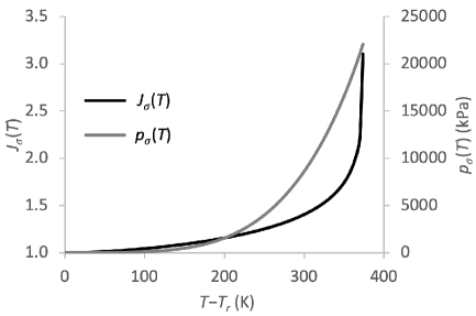
Figure 3.1. Plots of the volume ratio $J_{\sigma}\left(T\right)$ and gauge pressure $p_{\sigma}\left(T\right)$ for liquid water on its saturation curve, using NIST data.

then interpolate them using piecewise cubic polynomials and differentiate them when necessary, using a suitable software package such as Mathematica (Wolfram Research Inc.). Using downloaded properties over a broad range of $P$ at selected values of $T$ in the range $T_{r}\leq T\leq T_{c}$ (where $T_{c}=647.1\,\text{K}$ is the critical temperature), we may fit (3.46) to $P-P_{r}$ versus $J-J_{\sigma}\left(T\right)$ at each $T$ to obtain $B_{1}\left(T\right)$ (with coefficients of determination in the range $0.99997\leq R^{2}\leq 1.00000$ for the various values of $T$) and $B_{2}\left(T\right)$ (with $0.99991\leq R^{2}\leq 1.00000$) for a virial expansion with $m=2$. Then, the discrete set of coefficients $B_{1}$ and $B_{2}$ may be fitted to polynomial functions of $T$ (Figure 3.2) to produce

(a)

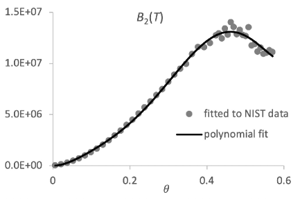
(b)

Figure 3.2. Virial coefficients $B_{1}\left(T\right)$ and $B_{2}\left(T\right)$ for liquid water, plotted against $\theta=1-T/T_{c}$. Symbols represent values obtained by fitting $p$ in equation (3.46) versus $J-J_{\sigma}\left(T\right)$ at selected increments of temperature in the range $T_{r}\leq T\leq T_{c}$. Solid lines represents polynomial approximations of those values as given in equations (3.51) and (3.52).

$$\begin{aligned} B_{1}\left(T\right)&=9.59435\times 10^{7}\,\theta^{6}+8.95496\times 10^{7}\,\theta^{5}-1.37737\times 10^{8}\,\theta^{4}\\ &+7.36381\times 10^{7}\,\theta^{3}-3.42044\times 10^{7}\,\theta^{2}\end{aligned}\,,$$ (3.51)

with $R^{2}=1.00000$ and

$$\begin{aligned} B_{2}\left(T\right)&=9.24187\times 10^{9}\,\theta^{6}-1.43932\times 10^{10}\,\theta^{5}+7.77799\times 10^{9}\,\theta^{4}\\ &-1.88532\times 10^{9}\,\theta^{3}+2.70511\times 10^{8}\,\theta^{2}\end{aligned}\,,$$ (3.52)

with $R^{2}=0.99885$, where $\theta=1-T/T_{c}$ and $B_{1}\left(T\right)$ and $B_{2}\left(T\right)$ are unitless. The scatter observed in $B_{2}\left(T\right)$ for lower values of $T$ (higher values of $\theta$) arises from the greater uncertainty in this parameter for this range of temperatures. These expressions may be differentiated as needed in (3.48). Using downloaded values of $c_{v\sigma}\left(T\right)$ on the saturation curve, we then evaluate $a_{\sigma}^{\prime\prime}\left(T\right)$ from (3.50) and integrate it twice to solve for $s_{\sigma}\left(T\right)$ and $a_{\sigma}\left(T\right)$, subject to the condition that $s_{r}=0$ and $a_{r}=0$ at the triple point (Figure 3.3). A comparison of these results against NIST data entries yields errors ranging from $-0.14\%$ to $0\%$ for $a_{\sigma}\left(T\right)$ and from $-1.30\%$ to $0\%$ for $s_{\sigma}\left(T\right)$, with the largest magnitudes occurring in the vicinity of $T_{c}$. With these functions, we may now calculate $a$ and $s$ for any $\left(T,J\right)$ using (3.47) and (3.48), allowing us to further verify the accuracy of our constitutive model (3.47) for liquid water against the NIST values as obtained from standard methods [38]. For $T_{r}\leq T\leq 643.15\,\text{K}$ and $0.9\leq p\leq 22\,000\,\text{kPa}$, we find that the error against NIST data ranges from $-0.74\%$ to $0.56\%$ for $a\left(T,J\right)$ ($0.00\pm 0.06\,\%$ mean±standard deviation) and from $-1.52\%$ to $0.05\%$ for $s\left(T,J\right)$ ($-0.02\pm 0.08\,\%)$. Similarly good agreement is found for the specific internal energy $u\left(T,J\right)$ ($-2.12\%$ to $0.05\%$, $-0.02\pm 0.11\>\%$) and specific enthalpy $h\left(T,J\right)$ ($-2.06\%$ to $0.41\%$, $-0.02\pm 0.12\,\%$). These small errors imply that the formulation of the constitutive model for liquids in this study is valid; small discrepancies with NIST data arise most likely from the simplistic choices of interpolation and approximation functions adopted in this illustrative example.

(a)

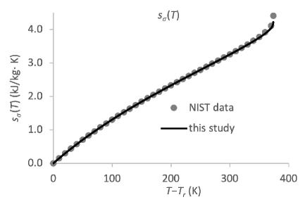
(b)

Figure 3.3. (a) Specific free energy $a_{\sigma}\left(T\right)$ and (b) specific entropy $s_{\sigma}\left(T\right)$ of liquid water on the saturation curve, evaluated from the method of this study (solid lines) and compared to NIST values (symbols).

3.7. Interface Jump Conditions

Interface jump conditions are needed to impose valid boundary conditions in any boundary value problem in continuum mechanics [24, 27, 23]. These jump conditions are derived from the same balance axioms that produce the governing differential equations. In some applications, the interface represents a material region, such as a membrane or shell domain separating two fluids, while in other cases it is an immaterial surface, such as the phase boundary between liquid and gas phases of a fluid, a shock wave in a compressible fluid, or an imaginary section through a material. In Appendix A, we derive interface jump conditions for immaterial interfaces that may move and deform, and we neglect certain effects, such as surface tension and its rate of work, that may occur due to disruption in intermolecular bonds introduced by the presence of such interfaces. These jump conditions are derived under the assumption that the interface separates two domains that each contains a single phase of the same substance. The phase may be the same on both sides of the interface, in which case the interface is permeable to the material. If the phases are different, the interface is assumed to be impermeable. Later, we generalize interface jump conditions to account for phase transformations on a phase boundary.

3.7.1. Summary of Jump Conditions

Jump conditions are derived under the assumption that the interface $\Gamma$ separates two domains denoted by $V_{+}$ and $V_{-}$. The velocity of $\Gamma$ is $\mathbf{v}^{\Gamma}$ and the unit normal on $\Gamma$ is $\mathbf{n}^{\Gamma}$, pointing away from $V_{+}$. For any quantity $f$, the expression $\left[\left[f\right]\right]\equiv f_{+}-f_{-}$ represents the jump in $f$ across $\Gamma$, with $f_{\pm}$ representing the values of $f$ in $V_{\pm}$, on $\Gamma$. The jump condition derived from the axiom of mass balance is

$$\left[\left[\rho\mathbf{u}^{\Gamma}\right]\right]\cdot\mathbf{n}^{\Gamma}=0\,,$$ (3.53)

where

$$\mathbf{u}^{\Gamma}\equiv\mathbf{v}-\mathbf{v}^{\Gamma}\,.$$ (3.54)

Evidently, the mass balance jump in (3.53) simply enforces continuity of the mass flux across and normal to the interface $\Gamma$. It is noteworthy that the mass balance jump does not impose any constraint on the tangential component of the mass flux or the velocity. Indeed, any tangential constraint would need to depend on the specifics of a particular analysis. For example, if $\Gamma$ separates two solid materials that slide past each other, there is no requirement for enforcing continuity of tangential mass flux or velocity. If the two solids are glued together however, the nature of this problem provides a specific additional interface condition, namely the continuity of the velocity component tangential to the interface. For viscous fluids this is known as the no-slip condition; it is recognized to be an empirically validated condition.

For thermoelastic fluids, the jump condition on the axiom of momentum balance reduces to

$$\left[\left[p\mathbf{I}+\rho\mathbf{u}^{\Gamma}\otimes\mathbf{u}^{\Gamma}\right]\right]\cdot\mathbf{n}^{\Gamma}=\mathbf{0}\,.$$ (3.55)

This jump condition tells us that the sum of pressure and linear momentum flux across and normal to $\Gamma$ is conserved. The jump condition on the axiom of energy balance takes the form

$$\left[\left[\rho\left(h+\frac{1}{2}\mathbf{u}^{\Gamma}\cdot\mathbf{u}^{\Gamma}\right)\mathbf{u}^{\Gamma}+\mathbf{q}\right]\right]\cdot\mathbf{n}^{\Gamma}=0\,,$$ (3.56)

where $h\equiv u+p/\rho$. Thus, the concept of enthalpy emerges naturally from the jump condition on the energy. Since $p$ represents a gauge pressure, we refer to $h$ as the specific gauge enthalpy. Note that $\frac{1}{2}\rho\mathbf{u}^{\Gamma}\cdot\mathbf{u}^{\Gamma}$ is the kinetic energy density of the material relative to $\Gamma$; we may refer to it as the diffusive kinetic energy density across $\Gamma$. The jump condition (3.56) tells us that the flux of enthalpy and diffusive kinetic energy plus the heat flux across and normal to $\Gamma$ is conserved.

Finally, the jump condition on the axiom of entropy inequality is given by

$$\left[\left[\rho s\mathbf{u}^{\Gamma}+\frac{1}{T}\mathbf{q}\right]\right]\cdot\mathbf{n}^{\Gamma}\leq 0\,.$$ (3.57)

The entropy inequality jump enforces a constraint on the sum of entropy fluxes carried by mass convection and heat conduction, across and normal to $\Gamma$. Since we have already formulated the constraints (3.10) and (3.13) on the functions of state $s$ and $\mathbf{q}$ on either side of $\Gamma$, the entropy inequality jump (3.57) serves to place a constraint on the feasibility of processes across $\Gamma$, as illustrated next.

These jump conditions are standard in the continuum mechanics literature [24, 14, 27, 9, 23, 1].

3.7.2. Normal Shock Wave

This normal shock wave problem illustrates how jump conditions may be used to solve for one-dimensional steady flow of an ideal gas with constant specific heat capacity across a stationary shock wave. We apply the jump conditions for mass, momentum and energy across a non-reactive interface (the shock wave) which is permeable to the substance ($\mathbf{u}^{\Gamma}\cdot\mathbf{n}^{\Gamma}\neq 0$).

In our framework, $\rho_{r}$ and $T_{r}$ are invariant reference values for the gas on either side of $\Gamma$, therefore $\left[\left[\rho_{r}\right]\right]=0$ and $\left[\left[T_{r}\right]\right]=0$. Similar constraints apply to invariants $R$ and $M$. Substituting the ideal gas relations in (3.25) and Example 3 into the jump conditions of (3.53), (3.55) and (3.56) produces

$$\left[\left[\frac{1}{J}\mathbf{u}^{\Gamma}\right]\right]\cdot\mathbf{n}^{\Gamma}=0\,,$$ (3.58)

$$\left[\left[\frac{1}{J}\left(\frac{RT}{M}\mathbf{I}+\mathbf{u}^{\Gamma}\otimes\mathbf{u}^{\Gamma}\right)\right]\right]\cdot\mathbf{n}^{\Gamma}=\mathbf{0}\,,$$ (3.59)

$$\left[\left[\frac{\rho_{r}}{J}\left(c_{p0}\left(T-T_{r}\right)+\frac{1}{2}\mathbf{u}^{\Gamma}\cdot\mathbf{u}^{\Gamma}\right)\mathbf{u}^{\Gamma}+\mathbf{q}\right]\right]\cdot\mathbf{n}^{\Gamma}=0\,.$$ (3.60)

Consider one-dimensional steady flow across a stationary shock wave $\Gamma$ ($\mathbf{v}^{\Gamma}=\mathbf{0}$, so that $\mathbf{u}^{\Gamma}=\mathbf{v}$), with uniform temperatures $T_{+}$ upstream and $T_{-}$ downstream, such that $\mathbf{q}=\mathbf{0}$ (adiabatic conditions) in both domains, leading to $\left[\left[\mathbf{q}\right]\right]\cdot\mathbf{n}^{\Gamma}=0$. Let $T_{+}$, $v_{+}\equiv\mathbf{v}_{+}\cdot\mathbf{n}^{\Gamma}$ and $J_{+}$ be given and solve for the corresponding downstream variables $T_{-}$, $v_{-}$ and $J_{-}$. From the mass jump (3.58) we find that

$$\frac{1}{J_{+}}v_{+}=\frac{1}{J_{-}}v_{-}\,,$$ (3.61)

where $v_{-}=\mathbf{v}_{-}\cdot\mathbf{n}^{\Gamma}$. From the momentum jump (3.59), we find that

$$\frac{1}{J_{+}}\left(\frac{RT_{+}}{M}+v_{+}^{2}\right)=\frac{1}{J_{-}}\left(\frac{RT_{-}}{M}+v_{-}^{2}\right)\,.$$ (3.62)

From the energy jump (3.60), making use of (3.61) and (3.27),

$$\frac{R\gamma}{M\left(\gamma-1\right)}T_{+}+\frac{1}{2}v_{+}^{2}=\frac{R\gamma}{M\left(\gamma-1\right)}T_{-}+\frac{1}{2}v_{-}^{2}\,,$$ (3.63)

where $\gamma\equiv c_{p0}/c_{v0}$ is the specific heat capacity ratio. This system of quadratic equations admits two solutions, namely the trivial solution $J_{-}=J_{+}$, $T_{-}=T_{+}$ and $v_{-}=v_{+}$ (implying that there is no shock wave), and the following solution,

$$\begin{aligned} \frac{J_{-}}{J_{+}}&=\frac{\text{Ma}_{+}^{2}\left(\gamma-1\right)+2}{\text{Ma}_{+}^{2}\left(1+\gamma\right)}\\ \frac{T_{-}}{T_{+}}&=\frac{\left(2\gamma\text{Ma}_{+}^{2}-\gamma+1\right)\left(\text{Ma}_{+}^{2}\left(\gamma-1\right)+2\right)}{\text{Ma}_{+}^{2}\left(\gamma+1\right)^{2}}\\ \frac{v_{-}}{v_{+}}&=\frac{\text{Ma}_{+}^{2}\left(\gamma-1\right)+2}{\text{Ma}_{+}^{2}\left(1+\gamma\right)}\end{aligned}\,,$$ (3.64)

where

$$\text{Ma}_{+}^{2}=\frac{Mv_{+}^{2}}{\gamma RT_{+}}\,,\quad\text{Ma}_{-}^{2}=\frac{Mv_{-}^{2}}{\gamma RT_{-}}\,,$$ (3.65)

are the squares of Mach numbers upstream and downstream, respectively. This result, which reproduces the classical solution for a normal shock wave [31], illustrates the application of the jump conditions derived above to a canonical problem involving an interface. As is evident from the solution in (3.64), the temperature is not continuous across $\Gamma$. This observation is important because it clearly establishes that jump conditions do not necessarily enforce temperature continuity. We revisit this concept below when we analyze phase transformations across an interface $\Gamma$.

Using the function of state for the specific entropy $s$ of an ideal gas as given in (3.36), we find that the change in $s$ across the shock wave is given by

$$s_{+}-s_{-}=\left[\left[s\right]\right]=c_{v0}\left(\left(1-\gamma\right)\ln\frac{J_{-}}{J_{+}}-\ln\frac{T_{-}}{T_{+}}\right)\,.$$ (3.66)

In particular, when $\text{Ma}_{+}=1$ (i.e., when there is no shock wave) we find that $\left[\left[s\right]\right]=0$. Furthermore, a plot of $\left[\left[s\right]\right]/c_{v0}$ versus $\text{Ma}_{+}$ shows that it is positive when $\text{Ma}_{+}<1$ and negative when $\text{Ma}_{+}>1$ (Figure 3.4). Combining the mass jump condition for the mixture (3.53) with the entropy inequality jump (3.57) under our given assumption that $\left[\left[\mathbf{q}\right]\right]\cdot\mathbf{n}^{\Gamma}=0$ shows that we must satisfy $\left[\left[s\right]\right]\leq 0$ whenever the mass flux across the shock wave is positive ($\rho\mathbf{u}^{\Gamma}\cdot\mathbf{n}>0$). This means that the entropy must increase at the downstream side of the shock wave. We conclude that the entropy inequality requires that shock waves occur only when the upstream flow is supersonic, $\text{Ma}_{+}\geq 1$. In other words, the flow cannot spontaneously jump from subsonic to supersonic under the adiabatic 1D flow conditions of this problem, as has been demonstrated in the classical compressible flow literature [25]. This application of the jump condition for entropy inequality across a normal shock wave illustrates the significance of this constraint on interfacial processes.

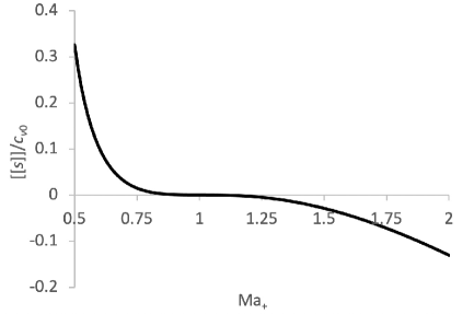
Figure 3.4. Plot of $\left[\left[s\right]\right]/c_{v0}$ across a normal shock wave, as a function of the upstream Mach number $\text{Ma}_{+}$ ($\gamma=1.4$). The entropy inequality jump (3.57) is only satisfied when $\text{Ma}_{+}\geq 1$.

4. Reactive Mixtures

Most thermodynamic applications deal with mixtures of multiple constituents, such as mixtures of gases, mixtures of the liquid and gas phases of a fluid, or solutions containing a solvent and solutes. To analyze such mixtures we may use the framework of mixture theory [36, 14, 8, 40, 1, 6]. This general framework can encompass a wide range of complexities, including phase changes, chemical reactions, diffusion of neutral or charged solutes, etc. In this study we choose to only consider phase transformations of a pure fluid substance across a boundary.

To formulate the jump condition for mass balance across a reactive interface $\Gamma$, we first need to present the axiom of mass balance for mixture constituents in a control volume. The basic concept of mixture theory is that any number of mixture constituents may be present in an elemental material region. In the context of a continuum framework, it is assumed mathematically that the size of this material region is infinitesimal; in other words, mathematically, all these materials coexist at a single point. In reality, the continuum model is a valid approximation only down to a representative scale of the microstructure. Thus, the elemental region should contain a sufficient number of molecules of the mixture constituents to obey the governing equations of the continuum framework.

In mixture theory we distinguish each mixture constituent $\alpha$ using a superscript, such as $\rho^{\alpha}$ for representing its apparent mass density, which represents the mass of constituent $\alpha$ per volume of the mixture. The general framework of mixture theory allows each constituent to follow a motion independent of others; thus, each constituent may have its own motion $\boldsymbol{\chi}^{\alpha}\left(\mathbf{X}^{\alpha},t\right)$ and velocity $\mathbf{v}^{\alpha}=\partial\boldsymbol{\chi}^{\alpha}/\partial t$.

4.1. Axiom of Mass Balance for Reactive Constituents

The material presented in this section can be found in classical mixture theory studies of reacting media [36, 24, 14, 8, 35, 27] and the more recent literature (such as [1, 6]). Since a mixture may involve reactions that exchange mass among its constituents (e.g., phase transformations, chemical reactions, etc.), the axiom of mass balance for each constituent $\alpha$ must account for this mass supply. The integral statement of mass balance in a fixed control volume $V$ takes the form

$$\frac{d}{dt}\int_{V}\rho^{\alpha}\,dV=-\int_{\partial V}\rho^{\alpha}\mathbf{v}^{\alpha}\cdot\mathbf{n}\,dS+\int_{V}\hat{\rho}^{\alpha}\,dV\,,$$ (4.1)

where $\mathbf{n}$ is the outward unit normal to the boundary $\partial V$ of $V$ and $\hat{\rho}^{\alpha}$ is the mass density supply to constituent $\alpha$ due to reactions with all other mixture constituents. This mass density supply is a function of state that requires a constitutive model, which may take a different form for chemical reactions, phase transformations, etc. It has units of mass per volume, per time, and it is positive when mass is added to constituent $\alpha$, negative when mass is lost from that constituent, and zero in the absence of reactions involving constituent $\alpha$. Using the divergence theorem to convert the surface integral in (4.1) to a volume integral, we obtain the differential statement of mass balance for each constituent $\alpha$,

$$\frac{\partial\rho^{\alpha}}{\partial t}+\operatorname{div}\left(\rho^{\alpha}\mathbf{v}\right)=\hat{\rho}^{\alpha}\,.$$ (4.2)

A fundamental principle of mixture theory is that the mixture should obey the axioms of mass, momentum and energy balance of a single constituent (a pure substance in a single phase). Taking the sum of (4.2) over all $\alpha$ and equating it to (3.1) shows that the mixture density is $\rho=\sum_{\alpha}\rho^{\alpha}$, the mixture velocity is $\mathbf{v}=\sum_{\alpha}\rho^{\alpha}\mathbf{v}^{\alpha}/\rho$, and the mass density supplies must satisfy the constraint

$$\sum_{\alpha}\hat{\rho}^{\alpha}=0\,.$$ (4.3)

Thus, mass gained by products of a reaction must balance the mass lost from reactants to conserve the mass of the mixture.

We may now apply the methodology described in Appendix A to evaluate the mass balance jump condition for each constituent $\alpha$, recognizing that $\hat{\rho}^{\alpha}$ in $V_{\epsilon}$ does not reduce to zero as $\epsilon\to 0$. In that case, the jump condition becomes

$$\left[\left[\rho^{\alpha}\left(\mathbf{v}^{\alpha}-\mathbf{v}^{\Gamma}\right)\right]\right]\cdot\mathbf{n}^{\Gamma}=-\bar{\rho}^{\alpha}\,.$$ (4.4)

Here, $\bar{\rho}^{\alpha}$ is the area density supply of mass to constituent $\alpha$ due to reactions taking place on $\Gamma$, such that

$$\lim_{\epsilon\to 0}\int_{V_{\epsilon}\left(t\right)}\hat{\rho}^{\alpha}\,dV=\lim_{\epsilon\to 0}\int_{\Gamma}\hat{\rho}^{\alpha}\,\epsilon\,dA=\int_{\Gamma}\bar{\rho}^{\alpha}\,dA\,.$$

Just as $\hat{\rho}^{\alpha}$ is a function of state in $V$, so is $\bar{\rho}^{\alpha}$ a function of state on $\Gamma$; it has units of mass flux (mass per area per time) and may also be described as the reactive mass flux of $\alpha$.

The mass balance jump is applied separately to each constituent $\alpha$. Moreover, the reactive mass flux $\bar{\rho}^{\alpha}$ satisfies the same type of constraint as $\hat{\rho}^{\alpha}$ in (4.3), namely

$$\sum_{\alpha}\bar{\rho}^{\alpha}=0\,.$$ (4.5)

4.2. Reaction Kinetics

Reaction kinetics and the stoichiometry of reacting mixtures have been described in the prior literature [7, 35, 29]. Reactions may occur among the constituents of a mixture which result in a temporal evolution of the mass content of reactants and products. A forward reaction between mixture constituents may be expressed as [29]

$$\sum_{\alpha}\nu_{R}^{\alpha}\mathcal{E}^{\alpha}\to\sum_{\alpha}\nu_{P}^{\alpha}\mathcal{E}^{\alpha}\,,$$ (4.6)

where $\mathcal{E}^{\alpha}$ is the material associated with constituent $\alpha$, $\nu_{R}^{\alpha}$ represents the stoichiometric coefficient of reactant $\alpha$ and $\nu_{P}^{\alpha}$ is that of the corresponding product. Similarly, a reversible reaction may be written as

$$\sum_{\alpha}\nu_{R}^{\alpha}\mathcal{E}^{\alpha}\rightleftharpoons\sum_{\alpha}\nu_{P}^{\alpha}\mathcal{E}^{\alpha}\,.$$ (4.7)

The summations are taken over all mixture constituents, though constituents that are not reactants in that particular reaction will have $\nu_{R}^{\alpha}=0$, and those that are not products will have $\nu_{P}^{\alpha}=0$.

Since the stoichiometric coefficients count the number of moles of reactants and products, we may relate the mass concentration $\rho^{\alpha}$ to the molar concentration $c^{\alpha}$ of constituent $\alpha$ via $\rho^{\alpha}=M^{\alpha}c^{\alpha}$, where $M^{\alpha}$ is the molar mass of $\alpha$. Similarly, we may define the molar density supply $\hat{c}^{\alpha}$ such that $\hat{\rho}^{\alpha}=M^{\alpha}\hat{c}^{\alpha}$. The stoichiometry of the reaction imposes constraints on the molar density supplies which may be represented by $\hat{c}^{\alpha}=\nu^{\alpha}\hat{\zeta}$, where $\hat{\zeta}$ is the molar production rate for the reaction (units of mole per volume, per time), and $\nu^{\alpha}=\nu_{P}^{\alpha}-\nu_{R}^{\alpha}$ is the net stoichiometric coefficient of $\alpha$ in the reaction. Substituting these relations into the constraint (4.3) on mass supplies produces $\sum_{\alpha}M^{\alpha}\nu^{\alpha}=0$. This relation may be recognized as the classical requirement to balance the molar mass of reactants and products in a reaction.

For reactions taking place on an interface $\Gamma$, we may similarly define the reactive molar flux $\bar{\zeta}$ such that

$$\bar{\rho}^{\alpha}=\nu^{\alpha}M^{\alpha}\bar{\zeta}\,.$$ (4.8)

Substituting this relation into (4.5) reproduces the same stoichiometric balance equation given in the previous paragraph. The implication of (4.8) is that only one constitutive relation is needed for $\bar{\zeta}$ to uniquely define the reactive mass supplies $\bar{\rho}^{\alpha}$ for all constituents $\alpha$. In chemical kinetics, it is common to adopt the ‘law of mass action’ for the constitutive model of $\bar{\zeta}$ (or $\hat{\zeta}$).

5. Phase Transformations

Given our framework of reactive mixtures, we can model phase transitions across a phase boundary modeled as an interface $\Gamma$ under the assumption that the reactive mixture on either side of $\Gamma$ only contains one phase of the pure substance. The relations derived in this section are valid under general conditions of phase transformation kinetics. Phase equilibrium is only considered as a special, clearly identified case.

Let a phase transformation take place across an interface $\Gamma$ that separates two phases, $\mathcal{S}^{a}$ and $\mathcal{S}^{b}$, of the same pure substance $\mathcal{S}$, with the unit normal $\mathbf{n}^{\Gamma}$ of $\Gamma$ pointing away from the domain of $\mathcal{S}^{a}$ (i.e., phase $\mathcal{S}^{a}$ resides in $V_{+}$ and phase $\mathcal{S}^{b}$ resides in $V_{-}$, Figure A1). Since we have limited our derivations to thermoelastic fluids, $a$ and $b$ may interchangeably denote the liquid and vapor phases. Consider that the phase transformation reaction may proceed in either direction,

$$\mathcal{S}^{a}\rightleftharpoons\mathcal{S}^{b}\,.$$ (5.1)

Our goal is to apply the jump conditions presented in Sections 3.7 and 4.1, under the general assumption that each side of $\Gamma$ is a mixture of both phases, while recognizing that the apparent density of phase $\mathcal{S}^{a}$ is zero in the domain of $\mathcal{S}^{b}$ ($\rho_{+}^{a}=\rho^{a}$, $\rho_{-}^{a}=0$), and that of phase $\mathcal{S}^{b}$ is zero in the domain of $\mathcal{S}^{a}$ ($\rho_{-}^{b}=\rho^{b}$, $\rho_{+}^{b}=0$). Thus, the mixture density and velocity on the side of $\mathcal{S}^{a}$ are $\rho=\rho^{a}$ and $\mathbf{v}=\mathbf{v}^{a}$, respectively, and those on the side of $\mathcal{S}^{b}$ are $\rho=\rho^{b}$ and $\mathbf{v}=\mathbf{v}^{b}$, and we may forgo the use of subscripts $+$ and $-$.

Note that the derivations presented in Sections 5.1, 5.2 and 5.3 below revisit and extend the classical Stefan problem [33] as applied to fluid phase transformations. More recent investigations have also proposed to use jump conditions to analyze phase transformations in thermoelastic fluids, however some of those studies proved or assumed a priori that the temperature is continuous across the phase interface, therefore they recovered the classical relations for phase equilibrium [27, 15, 19, 23], whereas our presentation investigates general conditions for phase transformations, without assuming temperature continuity as explained in Section 5.4 below. Later studies in the recent literature [34, 16, 9, 12] did account for a temperature jump, though they did not follow the approach we present here, nor did they derive an expression for the phase transition mass flux or investigate experimental validations.

5.1. Mass Balance Jump

Since $\Gamma$ is the phase boundary, we treat it as an immaterial surface. Based on the stoichiometry of this reaction ($\nu^{a}=-1$, $\nu^{b}=+1$ in (5.1)), reactive mass fluxes $\bar{\rho}^{\alpha}$ ($\alpha=a,\,b$) must satisfy $\bar{\rho}^{a}+\bar{\rho}^{b}=0$, or $\bar{\rho}^{b}=-\bar{\rho}^{a}=M\bar{\zeta}$ according to (4.8), where $M$ is the molar mass of substance $\mathcal{S}$ and $\bar{\zeta}$ is the reactive molar flux, such that $M\bar{\zeta}$ is the net reactive mass flux from the forward reaction $\mathcal{S}^{a}\to\mathcal{S}^{b}$ and the reverse reaction $\mathcal{S}^{a}\leftarrow\mathcal{S}^{b}$. Thus, $\bar{\zeta}$ may be positive if the forward reaction dominates, negative when the reverse reaction dominates, or zero when the reversible reaction (5.1) has reached phase equilibrium. Here, we used the reactive molar flux $\bar{\zeta}$ to emphasize that one mole of phase $a$ has been exchanged with one mole of phase $b$ on $\Gamma$. Now, the mass balance jump for each phase is reduced from (4.4) to

$$\rho^{a}\left(\mathbf{v}^{a}-\mathbf{v}^{\Gamma}\right)\cdot\mathbf{n}^{\Gamma}=\rho^{b}\left(\mathbf{v}^{b}-\mathbf{v}^{\Gamma}\right)\cdot\mathbf{n}^{\Gamma}=M\bar{\zeta}\,.$$ (5.2)

The mixture densities $\rho^{a}$ and $\rho^{b}$ may be very different from each other (liquid versus vapor phases), implying that $\mathbf{v}^{a}$ may also be very different from $\mathbf{v}^{b}$. The phase boundary moves with normal velocity $\mathbf{v}^{\Gamma}\cdot\mathbf{n}^{\Gamma}$. By solving for $\mathbf{v}^{\Gamma}\cdot\mathbf{n}^{\Gamma}$ in both equations,

$$\mathbf{v}^{\Gamma}\cdot\mathbf{n}^{\Gamma}=\mathbf{v}^{a}\cdot\mathbf{n}^{\Gamma}-\frac{M\bar{\zeta}}{\rho^{a}}=\mathbf{v}^{b}\cdot\mathbf{n}^{\Gamma}-\frac{M\bar{\zeta}}{\rho^{b}}\,,$$ (5.3)

we also find that the normal component of the relative velocity between the two phases is

$$\left(\mathbf{v}^{a}-\mathbf{v}^{b}\right)\cdot\mathbf{n}^{\Gamma}=M\bar{\zeta}\left(\frac{1}{\rho^{a}}-\frac{1}{\rho^{b}}\right)\,,$$ (5.4)

which may also be written as

$$\left[\left[\mathbf{v}\right]\right]\cdot\mathbf{n}^{\Gamma}=M\bar{\zeta}\left[\left[\frac{1}{\rho}\right]\right]\,.$$ (5.5)

Example 5.

Consider that $\mathcal{S}^{a}$ is liquid water ($a=\ell$) and $\mathcal{S}^{b}$ is water vapor ($b=v$), such that the reaction represents the evaporation of water (hence, $\bar{\zeta}>0$ by assumption). Assume that the liquid is stationary ($\mathbf{v}^{\ell}=\mathbf{0}$) even while its boundary $\Gamma$ is receding as the water evaporates. From (5.3) we can solve for the receding velocity, $\mathbf{v}^{\Gamma}\cdot\mathbf{n}^{\Gamma}=-M\bar{\zeta}/\rho^{\ell}$. We also find from (5.4) that $\mathbf{v}^{v}\cdot\mathbf{n}^{\Gamma}=\left(\frac{1}{\rho^{v}}-\frac{1}{\rho^{\ell}}\right)M\bar{\zeta}$; since $\rho^{\ell}>\rho^{v}$ for liquid and vapor, the latter result shows that $\mathbf{v}^{v}\cdot\mathbf{n}^{\Gamma}>0$, i.e., the vapor water moves away from the liquid to make up for the increase in volume as liquid water transforms into vapor.

5.2. Momentum Balance Jump

For our choice of mixtures on both sides of the phase boundary $\Gamma$, the momentum jump condition (3.55) becomes

$$\left(p^{a}-p^{b}\right)\mathbf{n}^{\Gamma}+\underbrace{\rho^{a}\left(\mathbf{v}^{a}-\mathbf{v}^{\Gamma}\right)\cdot\mathbf{n}^{\Gamma}}_{=M\bar{\zeta}}\left(\mathbf{v}^{a}-\mathbf{v}^{\Gamma}\right)-\underbrace{\rho^{b}\left(\mathbf{v}^{b}-\mathbf{v}^{\Gamma}\right)\cdot\mathbf{n}^{\Gamma}}_{=M\bar{\zeta}}\left(\mathbf{v}^{b}-\mathbf{v}^{\Gamma}\right)=\mathbf{0}\,.$$

Taking the dot product of this expression with $\mathbf{n}^{\Gamma}$ and using the general relation of (5.4) produces the jump condition on the pressure,

$$\left[\left[p\right]\right]=-\left(M\bar{\zeta}\right)^{2}\left[\left[\frac{1}{\rho}\right]\right]\,.$$ (5.6)

This result shows that the jump in pressure results from differences in the densities of phases $\mathcal{S}^{a}$ and $\mathcal{S}^{b}$ of $\mathcal{S}$. It is also proportional to the square of the mass flux from the reaction. When $\rho^{b}<\rho^{a}$, we find that $p^{a}>p^{b}$. Thus, if $a$ is the liquid phase and $b$ is the vapor phase, the liquid pressure is higher than the vapor pressure regardless of the direction of the phase transformation (i.e., evaporation or condensation). At phase equilibrium ($M\bar{\zeta}=0$), there is no jump in pressure across $\Gamma$.

5.3. Energy Balance Jump

So far, no constraint has emerged on the continuity of $T$ across $\Gamma$. The same argument applies to the gradient $\mathbf{g}$ of $T$, implying that the heat flux $\mathbf{q}$ may exhibit a discontinuity across $\Gamma$. Now, the energy jump may be reduced from (3.56) to

$$M\bar{\zeta}\left[\left[h+\frac{1}{2}\mathbf{u}^{\Gamma}\cdot\mathbf{u}^{\Gamma}\right]\right]+\left[\left[\mathbf{q}\right]\right]\cdot\mathbf{n}^{\Gamma}=0\,,$$ (5.7)

where $\left[\left[h\right]\right]=h^{a}-h^{b}$ and $\left[\left[\mathbf{q}\right]\right]=\mathbf{q}^{a}-\mathbf{q}^{b}$. This form of the energy jump condition shows that when $M\bar{\zeta}=0$ there can be no jump in the heat flux, $\left[\left[\mathbf{q}\right]\right]\cdot\mathbf{n}^{\Gamma}=0$. In other words, the heat flux is continuous across $\Gamma$, $\mathbf{q}^{a}\cdot\mathbf{n}^{\Gamma}=\mathbf{q}^{b}\cdot\mathbf{n}^{\Gamma}$, only at phase equilibrium. This is consistent with our expectation that a phase transformation requires the exchange of energy in the form of heat.

Since $h=u+p/\rho$ in general, we may also write

$$\left[\left[h\right]\right]=\left[\left[u\right]\right]+\left[\left[\frac{p}{\rho}\right]\right]=\left[\left[u\right]\right]+\frac{1}{\rho^{\Gamma}}\left[\left[p\right]\right]+p^{\Gamma}\left[\left[\frac{1}{\rho}\right]\right]\,,$$ (5.8)

where

$$\frac{1}{\rho^{\Gamma}}\equiv\frac{1}{2}\left(\frac{1}{\rho^{a}}+\frac{1}{\rho^{b}}\right)\,,\quad p^{\Gamma}\equiv\frac{1}{2}\left(p^{a}+p^{b}\right)\,$$ (5.9)

may be viewed as the respective values of $1/\rho$ and $p$ on $\Gamma$. Using the jump condition on the pressure found in (5.6), this expression for $\left[\left[h\right]\right]$ may be rewritten as

$$\left[\left[h\right]\right]=\left[\left[u\right]\right]+\left(p^{\Gamma}-\frac{1}{\rho^{\Gamma}}\left(M\bar{\zeta}\right)^{2}\right)\left[\left[\frac{1}{\rho}\right]\right]\,.$$ (5.10)

Now consider that there is no slip between the two phases $\mathcal{S}^{a}$ and $\mathcal{S}^{b}$ on $\Gamma$, so that $\mathbf{u}^{\Gamma}=\left(\mathbf{u}^{\Gamma}\cdot\mathbf{n}^{\Gamma}\right)\mathbf{n}^{\Gamma}$ (i.e., the tangential component of $\mathbf{u}^{\Gamma}$ on $\Gamma$ is zero). In that case, we may use the mass jump condition (5.2) and the relations of (5.9) to get

$$\left[\left[\frac{1}{2}\mathbf{u}^{\Gamma}\cdot\mathbf{u}^{\Gamma}\right]\right]=\frac{1}{\rho^{\Gamma}}\left(M\bar{\zeta}\right)^{2}\left[\left[\frac{1}{\rho}\right]\right]\,.$$ (5.11)

It follows from this result and (5.14) that

$$\left[\left[h+\frac{1}{2}\mathbf{u}^{\Gamma}\cdot\mathbf{u}^{\Gamma}\right]\right]=\left[\left[u\right]\right]+p^{\Gamma}\left[\left[\frac{1}{\rho}\right]\right]\,,$$ (5.12)

so that the jump condition (5.7) on the energy balance may be rewritten in its final form as

$$M\bar{\zeta}\left(\left[\left[u\right]\right]+p^{\Gamma}\left[\left[\frac{1}{\rho}\right]\right]\right)+\left[\left[\mathbf{q}\right]\right]\cdot\mathbf{n}^{\Gamma}=0\,.$$ (5.13)

By definition, the specific latent heat $L$ for the phase transformation of $\mathcal{S}^{a}$ into $\mathcal{S}^{b}$ is the ratio of the net heat flux across the phase boundary, $\left[\left[\mathbf{q}\right]\right]\cdot\mathbf{n}^{\Gamma}$, to the mass flux $M\bar{\zeta}$ produced in the phase transformation,

$$L=-\left(\left[\left[u\right]\right]+p^{\Gamma}\left[\left[\frac{1}{\rho}\right]\right]\right)=\frac{\left[\left[\mathbf{q}\right]\right]\cdot\mathbf{n}^{\Gamma}}{M\bar{\zeta}}\,.$$ (5.14)

The units of $L$ are those of energy per mass. Alternatively, we may define the molar latent heat of transformation as $\bar{L}=ML$. An important observation is that the definition of $L$ in (5.14) is valid for arbitrary processes.

Example 6.

Consider a phase transformation which takes place at a very slow, but non-zero rate $M\bar{\zeta}$. According to the momentum jump condition (5.6), in the limit when $M\bar{\zeta}\approx 0$, we find that

$$\left(M\bar{\zeta}\right)^{2}\left[\left[\frac{1}{\rho}\right]\right]=\left[\left[p\right]\right]\approx 0\,,$$ (5.15)

implying that $p^{a}\approx p^{b}\approx p^{\Gamma}$. In this limiting case it follows from (5.14) that

$$L_{0}=\lim_{M\bar{\zeta}\to 0}L=-\left[\left[h\right]\right]\,.$$ (5.16)

Thus, in the limit of phase transformation equilibrium, the specific latent heat is equal to the jump in enthalpy across $\Gamma$. Indeed, the specific latent heat of transformation is often called the specific enthalpy of formation. Generally, it is $L_{0}$ (not $L$) which is tabulated along with other thermodynamic properties of a substance. In this limiting case, we may estimate the slow reactive mass flux from

$$M\bar{\zeta}\approx-\frac{\left[\left[\mathbf{q}\right]\right]\cdot\mathbf{n}^{\Gamma}}{\left[\left[h\right]\right]}\,,$$ (5.17)

where $\left[\left[\mathbf{q}\right]\right]\cdot\mathbf{n}^{\Gamma}$ is evaluated from the knowledge of the temperature gradient and thermal conductivities in the domains on either side of $\Gamma$. The expression of (5.17) is the classical Stefan condition [33, 39].

Example 7.

Let $\mathcal{S}^{a}$ represent liquid water and $\mathcal{S}^{b}$ represent vapor water at phase equilibrium ($T^{\ell}=T^{v}$) and atmospheric pressure. The jump in enthalpy for water at these conditions is $\left[\left[h\right]\right]=h^{\ell}-h^{v}=-2256\,\text{kJ}/\text{kg}$. It follows from (5.16) that the specific enthalpy of evaporation is $L_{0}=2256\,\text{kJ}/\text{kg}$ at atmospheric pressure.

5.4. Entropy Inequality Jump

Using the above result (5.2) for the mass jump condition, the jump condition (3.57) on the entropy inequality across $\Gamma$ reduces to

$$M\bar{\zeta}\left[\left[s\right]\right]+\left[\left[\frac{1}{T}\mathbf{q}\right]\right]\cdot\mathbf{n}^{\Gamma}\leq 0\,,$$ (5.18)

where $\left[\left[s\right]\right]=s^{a}-s^{b}$. Since the ratio $\mathbf{q}/T$ emerges naturally in the entropy inequality, we may call it the thermal entropy flux. This constraint informs us of the circumstances under which a phase transformation may occur. Since $T$ and $\mathbf{q}$ may both be discontinuous across $\Gamma$, we can express the jump in thermal entropy flux in the direction normal to $\Gamma$ as

$$\left[\left[\frac{1}{T}\mathbf{q}\right]\right]\cdot\mathbf{n}^{\Gamma}=\frac{1}{T^{\Gamma}}\left[\left[\mathbf{q}\right]\right]\cdot\mathbf{n}^{\Gamma}+\left[\left[\frac{1}{T}\right]\right]\mathbf{q}^{\Gamma}\cdot\mathbf{n}^{\Gamma}\,,$$ (5.19)

where

$$\frac{1}{T^{\Gamma}}\equiv\frac{1}{2}\left(\frac{1}{T^{a}}+\frac{1}{T^{b}}\right)\,,\quad\mathbf{q}^{\Gamma}\equiv\frac{1}{2}\left(\mathbf{q}^{a}+\mathbf{q}^{b}\right)\,$$ (5.20)

represent the respective values of $1/T$ and $\mathbf{q}$ on $\Gamma$. Then (5.18) may be rewritten as

$$T^{\Gamma}M\bar{\zeta}\left[\left[s\right]\right]+\left[\left[\mathbf{q}\right]\right]\cdot\mathbf{n}^{\Gamma}+\left[\left[\frac{1}{T}\right]\right]T^{\Gamma}\mathbf{q}^{\Gamma}\cdot\mathbf{n}^{\Gamma}\leq 0\,,$$ (5.21)

where we have used the fact that $T^{\Gamma}>0$. Negating this inequality and adding it to the energy jump (5.13) to eliminate $\left[\left[\mathbf{q}\right]\right]\cdot\mathbf{n}^{\Gamma}$, yields the final general form of the constraint placed by the entropy inequality on phase transformations on the interface $\Gamma$,

$$M\bar{\zeta}\left(\left[\left[u\right]\right]+p^{\Gamma}\left[\left[\frac{1}{\rho}\right]\right]-T^{\Gamma}\left[\left[s\right]\right]\right)-\left[\left[\frac{1}{T}\right]\right]T^{\Gamma}\mathbf{q}^{\Gamma}\cdot\mathbf{n}\geq 0\,.$$ (5.22)

To better understand this non-trivial constraint it is beneficial to examine additional limiting cases. When the phase transformation reaction equilibrates ($M\bar{\zeta}=0$, implying $\left[\left[\mathbf{q}\right]\right]\cdot\mathbf{n}^{\Gamma}=0$ from the energy jump (5.13)), the constraint of (5.21) simplifies to

$$\left[\left[\frac{1}{T}\right]\right]\mathbf{q}^{\Gamma}\cdot\mathbf{n}^{\Gamma}\leq 0\,,\quad\text{at phase equilibrium}$$ (5.23)

where $\mathbf{q}^{\Gamma}\cdot\mathbf{n}^{\Gamma}=\mathbf{q}^{a}\cdot\mathbf{n}^{\Gamma}=\mathbf{q}^{b}\cdot\mathbf{n}^{\Gamma}$. Thus, if a jump in $T$ exists, it must satisfy this constraint whenever the heat flux $\mathbf{q}^{\Gamma}\cdot\mathbf{n}^{\Gamma}$ is non-zero; for example, if $\mathbf{q}^{\Gamma}\cdot\mathbf{n}^{\Gamma}>0$ (net heat flowing from the domain of $\mathcal{S}^{a}$ to the domain of $\mathcal{S}^{b}$) we must have $T^{a}>T^{b}$. However, when $\mathbf{q}^{\Gamma}\cdot\mathbf{n}^{\Gamma}=0$ (e.g., when $\mathbf{q}^{a}\cdot\mathbf{n}=\mathbf{q}^{b}\cdot\mathbf{n}=0$ as in the normal shock wave problem in Section 3.7.2), the sign of $\left[\left[1/T\right]\right]$ is inconsequential. Conversely, when the temperature is continuous across $\Gamma$ ($T^{a}=T^{b}$), the sign of $\mathbf{q}^{\Gamma}\cdot\mathbf{n}^{\Gamma}$ is inconsequential (i.e., the net heat flux may occur in either direction). We also conclude that continuity of the temperature across $\Gamma$ (i.e., $\left[\left[1/T\right]\right]=0$) is sufficient to satisfy the entropy inequality at phase equilibrium, but it is not a necessary condition. As is evident from (5.23) and the examples described in this paragraph, phase equilibrium may exist over a broad range of conditions.

Now, consider that a phase transformation occurs at very slow but non-zero rate $M\bar{\zeta}$ as defined in (5.17). It follows from the momentum jump condition (5.6) that $\left[\left[p\right]\right]\approx 0$. Consider that the phase transformation is taking place very close to the phase equilibrium state of the reversible reaction (5.1) and that $\left[\left[1/T\right]\right]\approx 0$ (i.e., assume that $T$ is continuous across $\Gamma$, consistent with the common assumption of phases transitions in the limit of reversibility). Now, (5.22) simplifies to

$$M\bar{\zeta}\left[\left[g\right]\right]\geq 0\,,\quad\text{near phase equilibrium}$$ (5.24)

where $g\equiv h-Ts$ is the definition of the specific Gibbs function (also called the specific free enthalpy, since $g=a+p/\rho$). In other words, the Gibbs function emerges naturally from the entropy inequality constraint during phase transformations on an interface $\Gamma$, in the limit as $M\bar{\zeta}\to 0$. The inequality (5.24) represents the thermodynamic constraint that must be satisfied by the constitutive models for $g^{a}$ and $g^{b}$ (and thus, the specific free energies $a^{a}$ and $a^{b}$) in order for the phase transformation to occur on $\Gamma$, at sufficiently slow rates $M\bar{\zeta}$, in the neighborhood of phase equilibrium. For the forward reaction $\mathcal{S}^{a}\to\mathcal{S}^{b}$ (with $\bar{\zeta}>0$), we must have $g^{a}\geq g^{b}$ according to (5.24); for the reverse reaction $\mathcal{S}^{b}\to\mathcal{S}^{a}$ ($\bar{\zeta}<0$), we must have $g^{a}\leq g^{b}$. In order for the phase transformation reaction to proceed slowly in either direction starting from the equilibrium state, we may argue that $\left[\left[g\right]\right]=0$ at phase equilibrium (even though this constraint is not strictly needed to satisfy (5.24) when $M\bar{\zeta}=0$ exactly). Therefore, continuity of the specific Gibbs function across the phase boundary is a sufficient condition for allowing phase transformations to initiate in either direction (forward or reverse), when the temperature is continuous across $\Gamma$. This thermodynamic requirement implies that the saturation curve between $\mathcal{S}^{a}$ and $\mathcal{S}^{b}$ may be identified as the line along which $\left[\left[g\right]\right]=0$ is satisfied simultaneously with $\left[\left[1/T\right]\right]=0$. This is a classical result of the thermodynamics of phase transformations; this presentation emphasizes the special set of conditions under which this result holds.

We may now argue that (5.23) describes the general spectrum of metastable phase equilibrium conditions, of which one special case, corresponding to $\left[\left[g\right]\right]=0$ and $\left[\left[1/T\right]\right]=0$, represents a stable phase equilibrium state, based on the reasoning outlined in the previous paragraph. It also bears to emphasize that the condition (5.24) that lets us identify the saturation curve is sufficient but not necessary for phase transformations to occur, as it does not represent the general case of allowable phase transformations, which are governed by (5.18) or its equivalent forms (5.21) and (5.22). A complete description of the kinetics of phase transformations requires the formulation of a constitutive model for the reactive mass flux $M\bar{\zeta}$, which must rely on experimental validation and simultaneously satisfy (5.18). Such a constitutive model is proposed further below. Prior to that however, now that we have established that $\left[\left[g\right]\right]=0$ and $\left[\left[1/T\right]\right]=0$ at stable phase equilibrium, we first need to clarify the relations between the reference free energies and entropies of the liquid and vapor phases.

To the best of our knowledge, the derivations presented in this section are original, as we could not find a similar presentation in the prior literature. They represent one of the major findings of this study.

5.5. Reference Configurations for Liquid and Vapor Phases

We are now ready to figure out how to set the reference configuration of liquid and vapor phases of a pure substance, taking into account the phase equilibrium conditions outlined in the previous section. Recall that we previously proposed constitutive relations for the specific free energy $a\left(T,J\right)$ of real gases (Section 3.6.2) and liquids (Section 3.6.3). In both cases we explained that we could evaluate $a\left(T,J\right)$ as well as the specific entropy $s\left(T,J\right)$ to within arbitrary constants $a_{r}$ and $s_{r}$, respectively. Now consider that we use these constitutive relations for the liquid and vapor phases of a pure substance, denoting their specific free energies as $a^{\ell}$ and $a^{v}$, respectively.

The proper way to set up a common reference configuration for the vapor and liquid phases of a pure substance is to select the same reference pressure $P_{r}$ and temperature $T_{r}$ for both phases. The most logical choice for a common reference is the triple point of the pure substance, where vapor, liquid and solid phases coexist, since this also allows us to account for phase transformations between the solid and liquid or the solid and vapor phases, as needed. We now need to determine the relation between $a_{r}^{v}$ and $a_{r}^{\ell}$ at the triple point. To figure it out, we use the phase equilibrium condition $\left[\left[g\right]\right]=0$ for the reversible phase transformation $\mathcal{S}^{\ell}\rightleftharpoons\mathcal{S}^{v}$ which was deduced in Section 5, evaluated specifically at the triple point. Recall that the specific Gibbs function is related to the specific free energy via $g=h-Ts=a+p/\rho$ where, in our approach, $p$ represents the gauge pressure. Since $p=0$ in the reference configuration (by definition), the jump condition $\left[\left[g_{r}\right]\right]=0$ reduces to $\left[\left[a_{r}\right]\right]=0$ at the triple point, which is equivalent to stating that

$$a_{r}^{\ell}=a_{r}^{v}\,.$$ (5.25)

Since this reference configuration is arbitrary, we can select $a_{r}^{\ell}=a_{r}^{v}=0$.

Remark 8.

In conventional thermodynamics where the absolute pressure $P$ is used instead of the gauge pressure, using $g=a+P/\rho$ and $\left[\left[g_{r}\right]\right]=0$ at the triple point would produce

$$a_{r}^{\ell}+\frac{P_{r}}{\rho_{r}^{\ell}}=a_{r}^{v}+\frac{P_{r}}{\rho_{r}^{v}}\,\text{conventional.}$$ (5.26)

Combining this result with the conventional choice of $a_{r}^{\ell}=0$ produces

$$a_{r}^{v}=P_{r}\left(\frac{1}{\rho_{r}^{\ell}}-\frac{1}{\rho_{r}^{v}}\right)\,\text{conventional.}$$ (5.27)

Thus, contrary to our gauge pressure approach, the referential free energies of liquid and vapor phases are not equal to each other in the classical framework, $\left[\left[a_{r}\right]\right]\neq 0$. In practice, this means that the specific free energy from our real gas constitutive model in Section 3.6.2 will deviate from the conventionally tabulated values $a^{v}=u^{v}-Ts^{v}$ by an amount comparable to or smaller in magnitude than the value of $a_{r}^{v}$ obtained from standard tables.

To determine the reference values $s_{r}^{v}$ and $s_{r}^{\ell}$ for the specific entropies, we examine the jump condition on the energy balance in the limit as the phase transformation approaches equilibrium. As shown in (5.16), we find that the latent heat of transformation, in the limit as the phase transformation reaction equilibrates, is equal to the jump in enthalpy, $\left[\left[h\right]\right]=-L_{0}$. Using the gauge enthalpy $h=u+p/\rho$, we can examine this jump condition at the triple point reference configuration, where $p=0$, so that

$$L_{r}=-\left[\left[u_{r}\right]\right]=u_{r}^{v}-u_{r}^{\ell}=\underbrace{a_{r}^{v}-a_{r}^{\ell}}_{=-\left[\left[a_{r}\right]\right]=0}+T_{r}\underbrace{\left(s_{r}^{v}-s_{r}^{\ell}\right)}_{=-\left[\left[s_{r}\right]\right]}\,,$$ (5.28)

where $L_{r}$ is the latent heat of evaporation near phase equilibrium at the triple point. If we let $s_{r}^{\ell}=0$ as is the convention, then $s_{r}^{v}=L_{r}/T_{r}$. Thus, unlike the referential specific free energy, the jump in referential specific entropy is not generally equal to zero in our gauge pressure approach. The evaluation of $s_{r}^{v}$ is contingent on the experimental measurement of $L_{r}$. Importantly, a single measurement of the latent heat of evaporation (e.g., $L_{r}$ at the triple point) is sufficient to predict $L_{0}$ along the entire saturation curve.

Remark 9.

In classical thermodynamics we use $h=u+P/\rho$ to evaluate the specific enthalpy. Thus, at the triple point reference configuration we would have

$$L_{r}=u_{r}^{v}-u_{r}^{\ell}+P_{r}\left(\frac{1}{\rho_{r}^{v}}-\frac{1}{\rho_{r}^{\ell}}\right)=\underbrace{a_{r}^{v}-a_{r}^{\ell}+P_{r}\left(\frac{1}{\rho_{r}^{v}}-\frac{1}{\rho_{r}^{\ell}}\right)}_{=-\left[\left[g_{r}\right]\right]=0}+T_{r}\left(s_{r}^{v}-s_{r}^{\ell}\right)\,,\,\text{conventional}$$ (5.29)

where we used the phase equilibrium condition $\left[\left[g_{r}\right]\right]=0$ at the triple point, with the classical definition of $g_{r}=a_{r}+P_{r}/\rho_{r}$. Comparing (5.28) to (5.29), it becomes evident that the result from our gauge pressure approach for the jump $\left[\left[s\right]\right]$ across the saturation curve is the same as in the conventional approach. It follows from a similar argument using (5.16) that the jump in enthalpy $\left[\left[h\right]\right]=h^{\ell}-h^{v}$ across the saturation curve has the same value in conventional thermodynamics (where absolute pressure is used) and our approach (where gauge pressure is used).

(a)

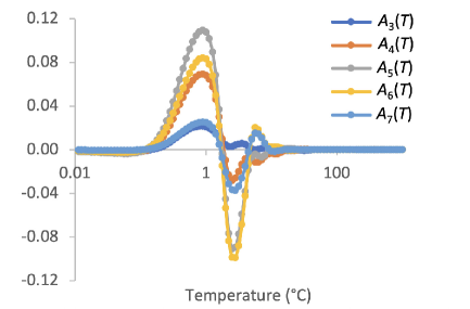
(b)

Figure 5.1. Virial coefficients $A_{1-7}\left(T\right)$ for water vapor, plotted against the temperature in °C on a logarithmic scale. Symbols represent values obtained by fitting $p/P_{r}$ in equation (3.40) versus $\frac{T}{JT_{r}}-1$ to pressure data downloaded from NIST, at selected temperatures in the range $0.01$ to $1000\,\text{\textdegree C}$. Solid curves represent interpolations of those coefficients.

Example 10.

As done in Example 4 with liquid water, we download the properties of water vapor at various pressures and temperatures (https://webbook.nist.gov/chemistry/fluid/) and fit the virial expansion (3.40) for the pressure in real gases to this data set to obtain discrete values of the virial coefficients $A_{k}\left(T\right)$ at selected values of $T$ in the range $0.01-1000\,{{}^{\circ}}\text{C}$. These discrete sets are then interpolated using piecewise cubic polynomials and differentiated as needed. By trial and error, it is determined that seven virial coefficients ($m=7$ in (3.40)) can accurately reproduce the response of water vapor (Figure 5.1). Similarly, we download the isobaric specific heat capacity $c_{pr}\left(T\right)$ at the triple-point pressure $P_{r}$ for the same range of temperatures and use those values to integrate $a_{0}^{\prime\prime}\left(T\right)$ in (3.43) twice with respect to $T$, assuming that $a_{r}^{v}=0$ and $s_{r}^{v}=L_{r}/T_{r}=9.15549341\,\text{kJ}/\text{kg}$, to obtain $s_{0}^{v}\left(T\right)$ in (3.44) and $a_{0}^{v}\left(T\right)$ in (3.45). We then evaluate $a^{v}\left(T,J\right)$ from (3.41) for any $\left(T,J\right)$, such as those on the saturation curve, and compare those values to the NIST-tabulated specific free energy (where $a_{r}^{v}=-125.994900\,\text{kJ}/\text{kg}$), showing that they initially deviate from each other, then become nearly identical at temperatures above $50\,\text{\textdegree C}$ (Figure 5.2a). We also evaluate $s^{v}\left(T,J\right)$ by substituting (3.41) into (3.10) and verify that its values along the saturation curve agree with the NIST-tabulated values (Figure 5.2b). We similarly compare our calculated specific internal energy $u^{v}=a^{v}+Ts^{v}$ on the saturation curve to the NIST-tabulated values, showing an initial deviation at temperatures below $50\,\text{\textdegree C}$ consistent with the difference noted in $a^{v}$ (Figure 5.3a). Finally, the specific gauge enthalpy $h^{v}=u^{v}+p^{v}/\rho^{v}$ is evaluated in our approach and compared to the tabulated value of the specific enthalpy, confirming that these measures are identical (Figure 5.3b).

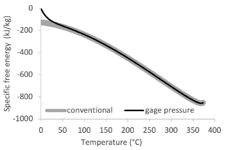
(a)

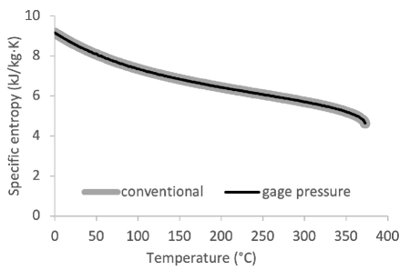
(b)

Figure 5.2. Thermodynamic properties of water vapor on the saturation curve, comparing conventional values from standard tables (NIST, https://webbook.nist.gov/chemistry/fluid/) to those evaluated in this study, where gauge pressure is used instead of absolute pressure. (a) The specific free energy $a^{v}$ in our approach starts from zero in the reference configuration (at the triple point), in contrast to the value from standard tables. (b) The specific entropy $s^{v}$ is identical in both approaches.

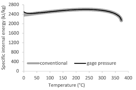
(a)

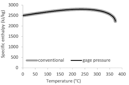
(b)

Figure 5.3. Thermodynamic properties of water vapor on the saturation curve, comparing conventional values from standard tables (NIST, https://webbook.nist.gov/chemistry/fluid/) to those evaluated in this study, where gauge pressure is used instead of absolute pressure. (a) The specific internal energy $u^{v}$ shows small differences for temperatures up to approximately $50\,\text{\textdegree C}$. (b) The enthalpy $h^{v}$ in the conventional approach is the same as the gauge enthalpy in the pressure gauge approach.

To the best of our knowledge, the presentation of this section represents an original literature contribution. In particular, our emphasis on using gauge pressure instead of absolute pressure is a distinction rarely addressed in the continuum mechanics and thermodynamics literature. Our approach emphasizes the cautionary distinctions that arise from using one or the other. Though readers may be concerned about our conclusion that the specific internal energy $u^{v}$ of the vapor phase of a thermoelastic fluid differs from entries in standard thermodynamic tables, this should be viewed as a minor concern since those standard tables also provide the enthalpy $h^{v}$ (whose values are the same as our gauge enthalpy), along with the absolute pressure $P^{v}$ and mass density $\rho^{v}$. Therefore, one can use the same standard thermodynamics tables to evaluate $u^{v}=h^{v}-\left(P^{v}-P_{r}\right)/\rho^{v}$ where $P_{r}$ is the triple point pressure, and recover the values of the specific internal energy $u^{v}$ of our formulation.

6. Phase Transformation Kinetics

6.1. Constitutive Model for Reactive Mass Flux

To complete the set of available equations, we need to propose a constitutive relation for the reactive mass flux $M\bar{\zeta}$. As reviewed by Persad and Ward [28], the standard models described in the literature are the Hertz-Knudsen or Hertz-Knudsen-Shrage relations, based on the kinetic theory of gases, and the statistical rate theory (SRT) expression for the evaporation flux. These authors also discussed the application of molecular dynamics to calculate the evaporation and condensation coefficients, which represent material parameters needed for the Hertz-Knudsen relation and its modifications. Badam et al. [4] proposed an alternative constitutive model for the evaporative flux based on phenomenological equations and Onsager’s reciprocal principle, also relying on the work of Bedeaux and Kjelstrup [5] which appealed to the concept of chemical potentials of the liquid and vapor phases at the interface.

Our goal here is to develop an original constitutive model for the reactive mass flux which is consistent with our continuum thermodynanics framework, without appealing to the kinetic theory of gases, molecular mechanisms, statistical approaches, or chemical potentials, since none of these concepts have emerged naturally from the governing equations presented so far. This constitutive model should reduce the mass flux to zero under the conditions that are consistent with phase equilibrium as outlined in the previous section. It must also satisfy the jump condition (5.18) or (5.22) on the entropy inequality. Based on these requirements, the simplest option is to let

$$M\bar{\zeta}=-\frac{1}{\left[\left[s\right]\right]}\left[\left[\frac{1}{T}\mathbf{q}\right]\right]\cdot\mathbf{n}^{\Gamma}\,.$$ (6.1)

In other words, the reactive mass flux for a phase transition on $\Gamma$ is proportional to the normal jump in thermal entropy flux, and inversely proportional to the jump in entropy. This choice of constitutive relation would satisfy the first requirement, since

$$\left[\left[\frac{1}{T}\mathbf{q}\right]\right]\cdot\mathbf{n}^{\Gamma}=\frac{1}{T^{\Gamma}}\underbrace{\left[\left[\mathbf{q}\right]\right]\cdot\mathbf{n}^{\Gamma}}_{=0}+\underbrace{\left[\left[\frac{1}{T}\right]\right]}_{=0}\mathbf{q}^{\Gamma}\cdot\mathbf{n}^{\Gamma}=0\quad\text{at phase equilibrium,}$$

when we consider phase equilibrium as the limiting condition leading to $\left[\left[g\right]\right]=0$ and $\left[\left[1/T\right]\right]=0$. This constitutive relation also satisfies the entropy inequality jump (5.18) without any residual dissipation. Consequently, we would describe the phase boundary as a non-dissipative interface for this choice of constitutive model. However, since non-zero heat fluxes $\mathbf{q}$ must exist on either side of $\Gamma$ to drive the phase transformation, the phase transition process is in fact irreversible (dissipative) when accounting for the domains of $\mathcal{S}^{a}$ and $\mathcal{S}^{b}$ across the interface $\Gamma$.

Since the entropy of the vapor phase of a substance is greater than that of the liquid phase, the term $-1/\left[\left[s\right]\right]$ in (6.1) is always positive whenever the $+$ side represents the liquid phase and the $-$ side is the vapor phase. Thus, the sign of the reactive mass flux $M\bar{\zeta}$ depends on the sign of $\left[\left[\mathbf{q}/T\right]\right]\cdot\mathbf{n}^{\Gamma}$; a positive value implies evaporation while a negative value implies condensation. It is also interesting to note that (6.1) predicts a singularity in the reactive mass flux as $\left[\left[s\right]\right]\to 0$ when the numerator is not zero (recall that $\left[\left[s\right]\right]$ depends only on temperatures and volumetric strains, whereas the numerator also depends on temperature gradients, implying that numerator and denominator are independent of each other). This singularity coincides with the emergence of the critical point in the liquid and vapor phases, where their entropy values are equal, as shown in a plot of the entropies of fluid water on the saturation curve (Figure 6.1). Thus, the model of (6.1) is consistent with the fact that liquid and vapor phases become indistinguishable in the supercritical regime.

Figure 6.1. The entropies of liquid and vapor water on the saturation curve (NIST, https://webbook.nist.gov/chemistry/fluid/) converge toward each other as the temperature rises to the critical point ($373.946\,\text{\textdegree C}$), showing that their difference $\left[\left[s\right]\right]$ reduces to zero at that point. This convergence produces a singularity in the constitutive model (6.1) for the phase transformation mass flux $M\bar{\zeta}$, consistent with the disappearance of the phase boundary in the supercritical regime.

Based on the alternative form of the residual dissipation in (5.22), we may also write the constitutive relation (6.1) as

$$M\bar{\zeta}=\frac{\left[\left[\frac{1}{T}\right]\right]T^{\Gamma}\mathbf{q}^{\Gamma}\cdot\mathbf{n}^{\Gamma}}{\left[\left[u\right]\right]+p^{\Gamma}\left[\left[\frac{1}{\rho}\right]\right]-T^{\Gamma}\left[\left[s\right]\right]}\,.$$ (6.2)

This equivalent alternative form makes it evident that a reactive mass flux for phase transformation can only occur in the presence of a non-zero temperature jump, $\left[\left[\frac{1}{T}\right]\right]\neq 0$, and a non-zero average heat flux, $\mathbf{q}^{\Gamma}\cdot\mathbf{n}^{\Gamma}\neq 0$, for this choice of constitutive relation.

Substituting this constitutive model into the expression for the specific latent heat $L$ in (5.14) produces

$$L=-\left[\left[s\right]\right]\frac{\left[\left[\mathbf{q}\right]\right]\cdot\mathbf{n}^{\Gamma}}{\left[\left[\frac{1}{T}\mathbf{q}\right]\right]\cdot\mathbf{n}^{\Gamma}}=-\left[\left[s\right]\right]\left(\frac{1}{T^{\Gamma}}+\left[\left[\frac{1}{T}\right]\right]\frac{\mathbf{q}^{\Gamma}\cdot\mathbf{n}^{\Gamma}}{\left[\left[\mathbf{q}\right]\right]\cdot\mathbf{n}^{\Gamma}}\right)^{-1}\,.$$ (6.3)

In the limit of phase equilibrium $\left[\left[g\right]\right]=0$ and $\left[\left[1/T\right]\right]=0$, the right-hand-side of this expression reduces to $L_{0}=-\left[\left[h\right]\right]$ in (5.16) from the fact that $g=h-Ts$, such that phase equilibrium implies $\left[\left[h\right]\right]=T^{\Gamma}\left[\left[s\right]\right]$. More generally, the expression of (6.3) shows that the specific latent heat $L$ may deviate substantially from $L_{0}$ for general phase transition processes.

To determine the temperature jump across $\Gamma$ under general conditions, we need to solve the field equations (the kinematic constraint (2.2), the momentum balance (3.3), and the energy balance in (3.19)) in both phases across $\Gamma$, and use the momentum and energy jumps in (3.55) and (3.56) as well as the constitutive relation of (6.1) as interface jump conditions. These interface conditions depend on the constitutive relations for $a\left(T,J\right)$ and $\mathbf{q}\left(T,J,\mathbf{g}\right)$ on either side of $\Gamma$, which have been formulated for each of the two phases $\mathcal{S}^{a}$ and $\mathcal{S}^{b}$ of the pure substance $\mathcal{S}$ independently of these interface jump conditions. Thus, jump conditions can only be satisfied for specific pairs of state variables $\left(T^{a},J^{a},\mathbf{g}^{a}\right)$ and $\left(T^{b},J^{b},\mathbf{g}^{b}\right)$.

To the best of our knowledge, the prior literature on continuum thermodynamics has not proposed a constitutive model for the phase transformation mass flux of the type given in (6.1). Therefore, all of the material presented in this section represents an original contribution. This model requires experimental and numerical validations to establish some measure of confidence in its validity. Since the model is predicated on the existence of a temperature jump across the phase boundary, we may reference experimental studies that have reported such temperature jumps under controlled conditions of a liquid-vapor phase transformation.

6.2. Experimental Validation

Persad and Ward [28] have tabulated an extensive set of results for the evaporation of water and ethanol under conditions that produce a temperature jump. However, these tabulated results do not include measurements of the temperature gradient $\mathbf{g}$ or heat flux $\mathbf{q}$ on the liquid and vapor sides of the phase boundary $\Gamma$, preventing us from using them to validate the model of (6.1). However, Badam et al. [4] provided a comprehensive set of experimental measurements relevant to the constitutive model in (6.1) or its equivalent form (6.2). These authors investigated the steady-state evaporation of water under various temperature and pressure conditions, where they found a temperature jump as high as $15.68\,\text{K}$ as they increased the vapor phase heating. In addition to measurements of the evaporative mass flux $M\bar{\zeta}$, temperatures across $\Gamma$, and the vapor pressure, they also measured temperature gradients on the liquid and vapor sides and computed the heat fluxes using thermal conductivities.

Badam et al.’s experiments were conducted at an average gauge pressure $p^{v}$ of $-100\,\text{Pa}$, with liquid water temperatures $T^{\ell}$ averaging $269.5\,\text{K}$ and water vapor temperatures $T^{v}$ averaging $277.4\,\text{K}$ [4]. Since their measurements remained close to the triple point of water, it is reasonable to assume that the entropy of liquid water was negligible compared to that of the vapor, such that the entropy jump appearing in (6.2) could be approximated as $\left[\left[s\right]\right]\approx-s^{v}$. Consequently, our constitutive model (6.1) may be reduced to the simplified form

$$\left[\left[\frac{q_{n}}{T}\right]\right]=\frac{q_{n}^{\ell}}{T^{\ell}}-\frac{q_{n}^{v}}{T^{v}}\approx s^{v}M\bar{\zeta}\,,$$ (6.4)

where $q_{n}^{\ell}=\mathbf{q}^{\ell}\cdot\mathbf{n}^{\Gamma}$ and $q_{n}^{v}=\mathbf{q}^{v}\cdot\mathbf{n}^{\Gamma}$ denote the heat flux components normal to the phase boundary in the liquid and vapor phases, respectively. Thus, as long as relative variations in $s^{v}$ remain small over the range of experimental conditions in the vapor phase, this constitutive model predicts a nearly linear relationship between $\left[\left[q_{n}/T\right]\right]$ and the evaporative flux $M\bar{\zeta}$. When we plot Badam et al.’s reported $\left[\left[q_{n}/T\right]\right]$ versus $M\bar{\zeta}$, we find a very strong linear relationship with a coefficient of determination $R^{2}=0.9893$ and a slope $s^{v}=5876\,\text{J}/\text{kg}\cdot\text{K}$ with a standard deviation of $92\,\text{J}/\text{kg}\cdot\text{K}$ (Figure 6.2).

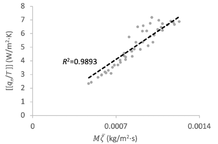
Figure 6.2. Plot of experimental data of Badam et al. [4] in the form of (6.4). A linear regression of the data produces $\left[\left[q_{n}/T\right]\right]=5876\,M\bar{\zeta}$ with a coefficient of determination $R^{2}=0.9893$.

The linear relationship strongly supports our proposed model for $M\bar{\zeta}$; however, the slope $5876\,\text{J}/\text{kg}\cdot\text{K}$ underestimates the entropy $s^{v}$ of water vapor in the range of their experimental conditions, which we estimate to average $9318\,\text{J}/\text{kg}\cdot\text{K}$ based on their reported $p^{v}$ and $T^{v}$ values (ranging from $9017$ to $9657\,\text{J}/\text{kg}\cdot\text{K}$). In effect, their experimental data underestimate our hypothesized theoretical value of the normal jump in thermal entropy flux $\left[\left[q_{n}/T\right]\right]$ by 37%, most likely due to the oversimplification of their experimental conditions using a one-dimensional analysis (i.e., using a mass flux $M\bar{\zeta}$ averaged over a curved $8\,\text{mm}\times 23\,\text{mm}$ liquid-vapor interface, while relying on measurements of temperature along a single centerline normal to that surface, see their Fig. 2).

7. Discussion

The objective of this study was to formulate the thermodynamics of phase transformations of a pure thermoelastic fluid using only a continuum approach. We used gauge pressure instead of absolute pressure in this framework, since the stress tensor in continuum mechanics is assumed to reduce to zero in some arbitrary reference configuration. This seemingly minor recognition had a major influence on our findings, as became evident in the development presented above. In Section 3.1, we presented the familiar differential statements for the axioms of mass, momentum and energy balance, which include functions of state for the fluid stress $\boldsymbol{\sigma}$, specific internal energy $u$, and heat flux $\mathbf{q}$. These functions of state model the behavior of specific fluids, and therefore they need to be described by constitutive relations. We proceeded to present the axiom of entropy inequality and adapted the concept presented by Coleman and Noll [11], namely that this inequality statement should be used to place constraints on the functions of state for arbitrary processes. The entropy inequality introduced the specific entropy $s$ as an additional function of state, and its combination with the energy balance, motivated by the need to eliminate user-specified specific heat supplies $r$ (as further elaborated upon in our recent study [3]), naturally produced the specific free energy $a$.

In Section 3.2, we proceeded to select a list of observable state variables suitable for the analysis of thermoelastic fluids, which included the temperature, volume ratio and temperature gradient. Given those state variables, we reviewed the constraints imposed on the functions of state using the entropy inequality. Using those constraints, we examined two alternative forms of the energy balance in Section 3.3, involving the material time derivative of temperature and specific entropy, respectively. The latter form could be used to better understand the concept of isentropic processes.

The volume ratio $J$ and the fluid velocity $\mathbf{v}$ may be obtained by solving the kinematic constraint of (2.2), concurrently with the differential statement of momentum balance in (3.3). For thermofluid analyses, the energy balance in (3.4) is also needed to solve for the temperature $T$. Though continuum analyses that employ the kinematic constraint (2.2) are not common in fluid mechanics, we have recently demonstrated that they can be used successfully to develop a general-purpose computational fluid dynamics finite element solver [2, 32]. To solve these equations in practice, we need constitutive relations for the relevant functions of state. Based on the constitutive restrictions presented in Section 3.2, the only functions of state that require constitutive relations are the specific free energy $a$ and the heat flux $\mathbf{q}$. Constitutive relations for all other functions of state can be derived from $a$.

In Section 3.6, we proceeded to formulate the constitutive relation for the specific free energy $a$ of ideal gases, real gases and liquids. As reviewed in that section, the resulting expressions we find for the specific free energy of ideal (3.31) and real (3.41) gases represent original contributions, since they appear to be the first to be derived starting from an expression for the gauge pressure $p$, instead of absolute pressure as in [27]. A virial expansion was similarly used to formulate the constitutive model for the specific free energy $a$ of liquids, as shown in (3.47). Since the forms of the constitutive models for the specific free energy of real liquids and gases presented in this study is novel, we demonstrated that it could reproduce standard thermodynamic properties of liquid water in Example 4, and vapor water in Example 10.

In Sections 3.7 and 4 we presented interface jump conditions for the axioms of mass, momentum and energy balance, and the axiom of entropy inequality, allowing for reactive mass exchanges across the interface. Jump conditions of this type have been derived previously in the continuum mechanics literature, including for reactive mixtures [24, 14, 23, 27, 1]. The specific free enthalpy function $h$ emerged naturally in the energy jump. As mentioned earlier in this presentation, this enthalpy function uses the gauge pressure $p$, instead of the absolute pressure $P$ as normally done in conventional thermodynamics.

Most significantly, the jump condition (3.57) on the entropy inequality can be used to enforce constraints on the thermodynamic feasibility of interfacial processes. We illustrated the application of this jump constraint to the case of a normal shock wave in Section 3.7.2, showing that it led to the common understanding that such a shock wave can only occur spontaneously (i.e., without the addition of heat) when supersonic flow transitions to subsonic flow [25]. Moreover, this example served as a useful reminder that temperature need not be continuous across an immaterial interface, even in the absence of a phase transformation.

The existence of temperature jumps across interfaces is accepted in the research literature but remains ambiguously defined in thermodynamics and heat transfer textbooks. In the thermodynamics of phase transition, textbooks typically emphasize that temperature and pressure remain continuous across the phase boundary. In heat transfer textbooks, the convective heat transfer formula between a solid and fluid assigns a different temperature to each side of their interface, though the fluid temperature is often described as the free stream temperature, generally implying that it is the temperature outside of the boundary layer located in the vicinity of the solid wall. Whether a temperature jump may exist on the interface is generally not discussed in those textbooks. A major objective of the current study was to eliminate this ambiguity entirely and provide the theoretical foundations that support the existence of a temperature jump, specifically in the case of a phase boundary.

In Section 5, we specialized the general jump conditions to the case of a reactive interface between the liquid and vapor phases of a pure substance. When applied to mass, momentum and energy balance, this specialization produced equations consistent with those of Stefan as he applied them to the investigation of the ice-liquid water interface [33, 39]. A detailed examination of the entropy jump led us to the conclusion that continuous temperature and pressure across the phase boundary is a sufficient condition for phase equilibrium ($M\bar{\zeta}=0$), though not necessary. By examining small disturbances in the mass flux $M\bar{\zeta}$ about this equilibrium, we concluded from (5.24) that phase equilibrium corresponds to continuity of the specific free enthalpy (the Gibbs function) across the phase boundary, consistent with classical concepts. This condition represented the first appearance of the specific free enthalpy function $g$ in this continuum thermodynamics formulation, implying that $g$ is only needed to identify phase equilibrium.

Upon establishing this continuity condition in the limiting case of phase equilibrium, we were able to determine how to relate the reference values $a_{r}$ for the specific free energy, and $s_{r}$ for the specific entropy, of liquid and vapor phases (Section 5.5). Whereas the liquid values of $a_{r}$ and $s_{r}$ were arbitrarily set to zero at the triple point, as done conventionally, the corresponding values for the vapor were derived from the continuity condition $\left[\left[g\right]\right]=0$. Contrary to the conventional approach, due to our use of gauge pressure $p$ instead of absolute pressure $P$, we found that $a_{r}$ for the vapor phase should also equal zero at the triple point. This led to a deviation of our thermodynamic values of $a$ from those calculated from conventional thermodynamic tables, by the value given in (5.27) at the triple point, though this deviation was not constant and became negligible with increasing temperature on the saturation curve, as illustrated for water in Figure 5.2. For this comparison, we evaluated $a=u-Ts$ from thermodynamic values of $u$ and $s$ reported in the NIST tables, since they do not report $a$ directly. As explained in Section 5.5, there were no differences in $s$ and $h$ between our values and standard tables, but the value of the specific internal energy $u$ exhibited the same pattern as $a$.

As a side note, taking the triple point as the reference configuration for the three phases of a pure substance is the logical choice when analyzing phase transformations. However, other applications, such as the analysis of reactive mixtures of liquids or gases, may employ an arbitrary (e.g., standard) reference configuration common to all mixture constituents, in order to properly evaluate the heat of reaction. Therefore, the existence of a triple point is not essential to the formulation of reactive mixture thermodynamics. It is just a convenient choice for the special case of phase transformations of a pure substance, which is the topic of this study.

To analyze more general cases of phase transformation kinetics, where the reactive mass flux is not negligibly small (i.e., irreversible thermodynamics of phase transformations), it became necessary to formulate a constitutive model for $M\bar{\zeta}$, using the entropy inequality jump (5.18) as a constraint on this choice of model. An examination of that jump condition showed that the only function of state which had not already been constrained by the axiom of entropy inequality in the liquid and vapor phases was the interfacial reactive mass flux $M\bar{\zeta}$. Given the simplicity of the expression in (5.18), and since the sign of $\left[\left[s\right]\right]$ remains fixed for an interface between liquid and vapor phases of a substance (e.g., as seen in Figure 6.1 at phase equilibrium), whereas $M\bar{\zeta}$ could be positive or negative, the constitutive relation presented in (6.1) was the self-evident form that would satisfy the entropy inequality, under the assumption that the interface is non-dissipative. In this relation, the direction of the mass flux (evaporation versus condensation) becomes contingent on the sign of the normal jump in thermal entropy flux, $-\left[\left[\mathbf{q}/T\right]\right]\cdot\mathbf{n}^{\Gamma}$.

To the best of our knowledge, this constitutive relation for the phase transition mass flux has not been proposed previously. By relying on temperature gradients on either side of the phase boundary, it deviates from conventional formulations that depend only on temperature and mass densities. The physical insight underlying this constitutive model is that the energy needed to cause evaporation or condensation (the latent heat of transformation) must be transported to the interface by the heat flux, (5.14), which must be a function of the temperature gradient according to the axiom of entropy inequality as presented in Section 3.4, thus it represents heat conduction. In contrast, standard textbook chemistry formulations for the heat of vaporization do not explicitly address how that energy is transported in the reacting medium or across the phase boundary. Textbook formulations typically assume that the temperature remains uniform in a process; as shown in Section 3.5, a state of uniform temperature for a pure thermoelastic fluid necessarily implies that all processes in that medium are reversible, thus lacking the generality of irreversible thermodynamics. We expect that the formulation presented in this study fills this important gap, in the context of a continuum framework.

Other investigators have previously used the jump conditions from mixture theory to examine phase transitions. For example, our derivations in Sections A.2, 5.2 and 5.3 show considerable analogy with the approach of Svendsen and Gray [34, 19], however these authors did not discuss the implications of these jump conditions as we do in Section 5.4, nor did they propose a constitutive model for the phase transition flux, as done in Section 6.1. Buratti et al. [9] also presented the same jump conditions across the phase interface as done in this study, but they adopted the assumption of temperature continuity early in their derivation. In contrast, Danescu [12] presented the same result as our equation (5.18) in Section 5.4, and based on the work of Fried and Shen [16] they identified what we called $T^{\Gamma}$ as the “equivalent temperature of the interface,” which they defined as a constitutive choice. Despite the close analogy of our approach with the prior work of Danescu [12], this author did not identify the interfacial phase transition mass flux as a function of state requiring a constitutive relation, such as the one we proposed in (6.1) or its equivalent form in (6.2).

To test the validity of our constitutive model against experimental data, we had access to the data set from the study of Badam et al. [4] which was the only one we could find that provided measurements of temperature gradients across the phase boundary (Gatapova et al. [17] also reported evaporative temperature jumps that depend on temperature gradients across the interface, but their experiments were conducted at the interface of liquid water and air). Using this data set with our model produced encouraging but mixed results: A very strong linear relation was observed between the model and experimental data in Figure 6.2, but the slope of the response underestimated the model by approximately 37%. While this outcome may tempt us to adjust the constitutive relation in (6.1) by including a positive scale factor less than or equal to unity, perhaps serving as some kind of material property for the phase transition mass flux, it is easy to show that this type of scaling would not satisfy the entropy inequality (5.18) under general conditions. It is more likely that the experimental conditions of Badam et al. [4] could not be reduced to a one-dimensional analysis. Indeed, a closer examination of their experimental results (not reported here) shows that they would also not satisfy the general energy jump (5.13), nor the classical Stefan energy jump condition (5.17), satisfactorily when assuming that one-dimensional conditions prevail. Therefore, more evidence is needed to support or reject the validity of our proposed constitutive model for the phase transformation mass flux.

If this constitutive relation is found to be valid, it would represent a powerful tool for analyzing phase transition kinetics under arbitrary conditions, including those that deviate significantly from phase equilibrium. As reviewed in Section 6.1, this constitutive model clearly establishes that phase transitions can only occur in the presence of a temperature jump, $\left[\left[1/T\right]\right]\neq 0$, where the heat flux entering the interface from one side differs from the heat flux leaving the interface on the opposite side, $\mathbf{q}^{\Gamma}\cdot\mathbf{n}^{\Gamma}\neq 0$. Evidently, the difference in heat flux across $\Gamma$ contributes to the specific latent heat of the phase transformation, as shown in (6.3). Thus, phase transformations always require a non-zero heat flux on either side of $\Gamma$, implying that this process is dissipative (irreversible), regardless of the fact that the immaterial phase interface $\Gamma$ itself is modeled as non-dissipative.

In summary, we have revisited fundamental concepts in the thermodynamics of pure fluids and their phase transformation, using only a continuum approach, with no reference to alternative frameworks such as statistical thermodynamics. We cited some of the classical and recent literature in the development of well-known fundamental principles and highlighted our novel contributions in the relevant sections, with further comparisons reported in the above paragraphs. While we recovered almost all the fundamental relations of classical thermodynamics, we found that a self-consistent framework should employ gauge pressure relative to a suitable reference configuration, instead of absolute pressure, when evaluating the specific free energy and its related functions of state. Using gauge pressure, we were also able to formulate a novel closed-form expression for the specific free energy of ideal gases, which served as the basis for related formulations for real gases and liquids using virial expansions. To examine phase transformation kinetics, we placed a special emphasis on the jump condition for the axiom of entropy inequality, which allowed us to recover the conventional result that phase equilibrium coincides with continuity of temperature, pressure, and free enthalpy across the phase boundary. These results were found to be consistent with the prior classical literature going back to the work of Stefan [33] and Gibbs [18], as well as the more recent continuum thermodynamic literature [23, 15, 34, 19, 16]. Moreover, this jump condition allowed us to formulate an original constitutive relation for arbitrary phase transition kinetics, showing that phase transformations must be accompanied by a jump in temperature across the phase boundary. Further experimental and computational evidence is needed to conclusively validate (or reject) this proposed constitutive model. This continuum framework is well suited for implementation in a computational framework, such as the finite element method [2, 32] and the phase field method [10]. Though not addressed explicitly in this study, the analysis of solid-fluid phase transformations may be easily extended from the presentation given here, by allowing the Cauchy stress tensor $\boldsymbol{\sigma}$ of the solid phase to depend on a suitable strain tensor, instead of just $J$.

A. Appendix

A.1. Derivation of Interface Jump Conditions

Let the interface $\Gamma$ move at a velocity $\mathbf{v}^{\Gamma}$ through the control volume $V$ and let the unit normal to $\Gamma$ be denoted by $\mathbf{n}^{\Gamma}$ (Figure A1). Our goal is to formulate the jump conditions for mass, momentum, energy and entropy across $\Gamma$, in terms of the values of state variables and functions of state on both sides of $\Gamma$. To achieve this goal, we define a region $V_{\epsilon}\left(t\right)$ about $\Gamma$ as the thin volume extending along $\pm\mathbf{n}^{\Gamma}$ by a total thickness $\epsilon$, with the remaining regions of $V$ denoted by $V_{+}$ and $V_{-}$ ($V=V_{+}\cup V_{-}\cup V_{\epsilon}$). The boundary surface between $V_{+}$ and $V_{\epsilon}$ is $\Gamma_{+}$, with its outward normal relative to $V_{+}$ given by $\mathbf{n}_{+}=\mathbf{n}^{\Gamma}$, and that between $V_{-}$ and $V_{\epsilon}$ is $\Gamma_{-}$ with outward normal relative to $V_{-}$ given by $\mathbf{n}_{-}=-\mathbf{n}^{\Gamma}$; the side surface of $V_{\epsilon}\left(t\right)$ is denoted by $\Gamma_{\epsilon}$, so that $\partial V_{\epsilon}=\Gamma_{+}\cup\Gamma_{-}\cup\Gamma_{\epsilon}$ represents the entire boundary of $V_{\epsilon}\left(t\right)$.

Let $f\left(\mathbf{x},t\right)$ represent a material density function defined in $V_{\epsilon}$; for example, $f$ may represent mass, momentum or internal and kinetic energy density of the material in $V_{\epsilon}$. An integral statement of $f$ over $V_{\epsilon}\left(t\right)$ may be evaluated in the limit as $\epsilon\to 0$ as

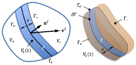
Figure A1. Interface jump conditions are defined across an interfacial surface $\Gamma$ and evaluated using axioms of conservation over a thin region $V_{\epsilon}\left(t\right)$ of thickness $\epsilon$ within the material, whose mid-surface is $\Gamma$. The interface $\Gamma$ moves with a velocity $\mathbf{v}^{\Gamma}$ and its surface normal is $\mathbf{n}^{\Gamma}$. The boundary $\partial V_{\epsilon}\left(t\right)$ is the union of the front surface $\Gamma_{+}$, the back surface $\Gamma_{-}$, and the side surface $\Gamma_{\epsilon}$. As $\epsilon\to 0$, $\Gamma_{+}$ and $\Gamma_{-}$ collapse onto $\Gamma$, whereas $\Gamma_{\epsilon}$ collapses onto the boundary contour curve $\partial\Gamma$ of $\Gamma$.

$$\lim_{\epsilon\to 0}\int_{V_{\epsilon}\left(t\right)}f\,dV=\lim_{\epsilon\to 0}\int_{\Gamma}f\,\epsilon\,dA=0\,,$$ (A.1)

since the elemental mass in $V_{\epsilon}$ goes to zero in that limit.

Now consider an integral statement of a function $\mathbf{f}\cdot\mathbf{n}_{\epsilon}$ on $\partial V_{\epsilon}$, where $\mathbf{n}_{\epsilon}$ is the outward normal to $\partial V_{\epsilon}$. For example, $\mathbf{f}\cdot\mathbf{n}_{\epsilon}$ may represent mass, momentum or internal and kinetic energy flux across the surface $\partial V_{\epsilon}$, positive in the outward direction to $\partial V_{\epsilon}$; it may also represent surface traction or its rate of work, or heat flux across $\partial V_{\epsilon}$. Note that $\mathbf{n}_{\epsilon}=-\mathbf{n}_{+}$ on $\Gamma_{+}$ and $\mathbf{n}_{\epsilon}=-\mathbf{n}_{-}$ on $\Gamma_{-}$. In that case,

$$\int_{\partial V_{\epsilon}}\mathbf{f}\cdot\mathbf{n}_{\epsilon}\,dA=-\int_{\Gamma_{+}}\mathbf{f}_{+}\cdot\mathbf{n}_{+}\,dA-\int_{\Gamma_{-}}\mathbf{f}_{-}\cdot\mathbf{n}_{-}\,dA+\int_{\Gamma_{\epsilon}}\mathbf{f}_{\epsilon}\cdot\mathbf{n}_{\epsilon}\,dA\,,$$ (A.2)

where $\mathbf{f}_{+}$, $\mathbf{f}_{-}$ and $\mathbf{f}_{\epsilon}$ are the values of $\mathbf{f}$ on $\Gamma_{+}$, $\Gamma_{-}$ and $\Gamma_{\epsilon}$, respectively. In the limit as $\epsilon\to 0$ we note that the surfaces $\Gamma_{+}$ and $\Gamma_{-}$ collapse onto $\Gamma$, so that $\mathbf{f}_{+}\cdot\mathbf{n}_{+}dA\to\mathbf{f}_{+}\cdot\mathbf{n}^{\Gamma}\,dA$ and $\mathbf{f}_{-}\cdot\mathbf{n}_{-}dA\to-\mathbf{f}_{-}\cdot\mathbf{n}^{\Gamma}\,dA$. On the lateral surface $\Gamma_{\epsilon}$, we note that the elemental area may be written as $dA=\epsilon\,ds$, where $ds$ is a path variable along the contour curve $\partial\Gamma$. Therefore, as $\epsilon\to 0$, the lateral surface shrinks to zero. For quantities proportional to mass flux (including momentum or internal and kinetic energy flux), this integral thus reduces to zero,

$$\lim_{\epsilon\to 0}\int_{\Gamma_{\epsilon}}\mathbf{f}_{\epsilon}\cdot\mathbf{n}_{\epsilon}\,dA=\lim_{\epsilon\to 0}\int_{\partial\Gamma}\epsilon\mathbf{f}_{\epsilon}\cdot\mathbf{n}_{\epsilon}\,ds=0\,.$$ (A.3)

For other quantities, such as surface traction $-p_{\epsilon}\mathbf{n}_{\epsilon}$, its rate of work $-p_{\epsilon}\mathbf{v}_{\epsilon}\cdot\mathbf{n}_{\epsilon}$, or heat flux $\mathbf{q}_{\epsilon}\cdot\mathbf{n}_{\epsilon}$ normal to $\Gamma_{\epsilon}$, we choose to neglect those contributions in our treatment here (which is equivalent to neglecting surface tension, surface energy, and heat leakage tangential to $\Gamma$). We may thus write the integral statement (A.2) in the limit as $\epsilon\to 0$ as

$$\lim_{\epsilon\to 0}\int_{\Gamma_{\epsilon}}\mathbf{f}\cdot\mathbf{n}_{\epsilon}\,dA=-\int_{\Gamma}\left[\left[\mathbf{f}\right]\right]\cdot\mathbf{n}^{\Gamma}\,dA\,,$$ (A.4)

where

$$\left[\left[\mathbf{f}\right]\right]\equiv\mathbf{f}_{+}-\mathbf{f}_{-}$$ (A.5)

represents the jump in $\mathbf{f}$ across $\Gamma$.

A.2. Mass Balance Jump

We now apply these identities to evaluate the mass balance jump across the interface $\Gamma$. We write the integral form of the axiom of mass balance over the thin domain $V_{\epsilon}\left(t\right)$, recognizing that $\partial V_{\epsilon}\left(t\right)$ moves with a velocity $\mathbf{w}_{\epsilon}$ such that the velocity of the material crossing $\partial V_{\epsilon}\left(t\right)$ is $\left(\mathbf{v}_{\epsilon}-\mathbf{w}_{\epsilon}\right)\cdot\mathbf{n}_{\epsilon}$,

$$\begin{aligned} \frac{d}{dt}\int_{V_{\epsilon}\left(t\right)}\rho\,dV&=-\int_{\partial V_{\epsilon}\left(t\right)}\rho\left(\mathbf{v}-\mathbf{w}\right)\cdot\mathbf{n}_{\epsilon}\,dA\\ &=\int_{\Gamma_{+}}\rho_{+}\left(\mathbf{v}_{+}-\mathbf{w}_{+}\right)\cdot\mathbf{n}_{+}\,dA+\int_{\Gamma_{-}}\rho_{-}\left(\mathbf{v}_{-}-\mathbf{w}_{-}\right)\cdot\mathbf{n}_{-}\,dA\\ &-\oint_{\partial\Gamma}\rho_{\epsilon}\left(\mathbf{v}_{\epsilon}-\mathbf{w}_{\epsilon}\right)\cdot\mathbf{n}_{\epsilon}\,\epsilon ds\end{aligned}\,,$$

Taking the limit as $\epsilon\to 0$, we find that $\mathbf{w}_{+}\to\mathbf{v}^{\Gamma}$ on $\Gamma_{+}\to\Gamma$ and $\mathbf{w}_{-}\to\mathbf{v}^{\Gamma}$ on $\Gamma_{-}\to\Gamma$, whereas the contour integral over $\partial\Gamma$ reduces to zero since the mass flux goes to zero, so that

$$0=\int_{\Gamma}\left[\left[\rho\left(\mathbf{v}-\mathbf{v}^{\Gamma}\right)\right]\right]\cdot\mathbf{n}^{\Gamma}\,d\Gamma\,.$$ (A.6)

Since the above condition must hold for arbitrary interfaces $\Gamma$, we conclude that the jump condition derived from the mass balance is satisfied pointwise on $\Gamma$ as given in (3.53).

A.3. Linear Momentum Balance Jump

Following the same procedure, we may write the integral form of the linear momentum balance over $V_{\epsilon}\left(t\right)$ as

$$\frac{d}{dt}\int_{V_{\epsilon}\left(t\right)}\rho\mathbf{v}\,dV=-\int_{\partial V_{\epsilon}\left(t\right)}\rho\mathbf{v}\otimes\left(\mathbf{v}-\mathbf{w}\right)\cdot\mathbf{n}_{\epsilon}\,dA-\int_{\partial V_{\epsilon}\left(t\right)}p\mathbf{n}_{\epsilon}\,dA+\int_{V_{\epsilon}\left(t\right)}\rho\mathbf{b}\,dV\,.$$ (A.7)

Taking the limit as $\epsilon\to 0$ produces

$$0=\int_{\Gamma}\left[\left[\rho\mathbf{v}\otimes\left(\mathbf{v}-\mathbf{v}^{\Gamma}\right)\right]\right]\cdot\mathbf{n}^{\Gamma}\,dA+\int_{\Gamma}\left[\left[p\right]\right]\mathbf{n}^{\Gamma}\,dA+0\,.$$ (A.8)

Since this integral statement must remain valid for arbitrary $\Gamma$, we may write

$$\left[\left[p\mathbf{I}+\rho\mathbf{v}\otimes\mathbf{u}^{\Gamma}\right]\right]\cdot\mathbf{n}^{\Gamma}=\mathbf{0}\,.$$ (A.9)

If we take the dyadic product of the mass balance jump in (3.53) with $\mathbf{v}^{\Gamma}$ and subtract it from the momentum jump above, we may rewrite it as shown in (3.55).

A.4. Energy Balance Jump

The integral statement of the axiom of energy balance over $V_{\epsilon}\left(t\right)$ is

$$\begin{aligned} \frac{d}{dt}\int_{V_{\epsilon}\left(t\right)}\rho\left(u+\frac{1}{2}\mathbf{v}\cdot\mathbf{v}\right)\,dV&=-\int_{\partial V_{\epsilon}\left(t\right)}\rho\left(u+\frac{1}{2}\mathbf{v}\cdot\mathbf{v}\right)\left(\mathbf{v}-\mathbf{w}\right)\cdot\mathbf{n}_{\epsilon}\,dV\\ &-\int_{\partial V_{\epsilon}\left(t\right)}p\mathbf{v}\cdot\mathbf{n}_{\epsilon}\,dA\\ &+\int_{V_{\epsilon}\left(t\right)}\rho\mathbf{b}\cdot\mathbf{v}\,dV-\int_{\partial V_{\epsilon}\left(t\right)}\mathbf{q}\cdot\mathbf{n}_{\epsilon}\,dA+\int_{V_{\epsilon}\left(t\right)}\rho r\,dV\end{aligned}\,.$$

In the limit as $\epsilon\to 0$ this expression reduces to

$$\begin{aligned} 0&=\int_{\Gamma}\left[\left[\rho\left(u+\frac{1}{2}\mathbf{v}\cdot\mathbf{v}\right)\left(\mathbf{v}-\mathbf{v}^{\Gamma}\right)\right]\right]\cdot\mathbf{n}^{\Gamma}\,dA\\ &+\int_{\Gamma}\left[\left[p\mathbf{v}\right]\right]\cdot\mathbf{n}^{\Gamma}\,dA\\ &+0+\int_{\Gamma}\left(\left[\left[\mathbf{q}\right]\right]\cdot\mathbf{n}^{\Gamma}\right)\,dA+0\end{aligned}\,.$$

This energy jump may now be rewritten as

$$\left[\left[\rho\left(u+\frac{1}{2}\mathbf{v}\cdot\mathbf{v}\right)\mathbf{u}^{\Gamma}+p\mathbf{v}+\mathbf{q}\right]\right]\cdot\mathbf{n}^{\Gamma}=0\,.$$ (A.10)

Multiply the mass balance jump in (3.53) by $\frac{1}{2}\mathbf{v}^{\Gamma}\cdot\mathbf{v}^{\Gamma}$ and subtract it from this expression; also subtract the dot product of the momentum balance jump in (3.55) with $\mathbf{v}^{\Gamma}$ to produce the relation of (3.56).

A.5. Entropy Inequality Jump

The integral statement of the axiom of entropy inequality over $V_{\epsilon}\left(t\right)$ is

$$\frac{d}{dt}\int_{V_{\epsilon}\left(t\right)}\rho s\,dV+\int_{\partial V_{\epsilon}\left(t\right)}\rho s\left(\mathbf{v}-\mathbf{w}\right)\cdot\mathbf{n}_{\epsilon}\,dA+\int_{\partial V_{\epsilon}\left(t\right)}\frac{1}{T}\mathbf{q}\cdot\mathbf{n}_{\epsilon}\,dA-\int_{V_{\epsilon}\left(t\right)}\rho\frac{r}{T}\,dV\geq 0\,.$$

In the limit as $\epsilon\to 0$ this expression reduces to

$$\begin{aligned} &0-\int_{\Gamma}\left[\left[\rho s\mathbf{u}^{\Gamma}\right]\right]\cdot\mathbf{n}^{\Gamma}\,dA\\ &-\int_{\Gamma}\left[\left[\frac{1}{T}\mathbf{q}\right]\right]\cdot\mathbf{n}^{\Gamma}\,dA-0\geq 0\end{aligned}\,.$$

This relation is valid for arbitrary $\Gamma$, thus it reduces to the expression in (3.57).

References

- [1] Gerard A Ateshian, On the theory of reactive mixtures for modeling biological growth, Biomech Model Mechanobiol 6 (2007), no. 6, 423–445.
- [2] Gerard A Ateshian, Jay J Shim, Steve A Maas, and Jeffrey A Weiss, Finite element framework for computational fluid dynamics in FEBio, J Biomech Eng 140 (2018), no. 2, 0210011–02100117.
- [3] Gerard A Ateshian and Brandon K Zimmerman, Continuum thermodynamics of constrained reactive mixtures, J Biomech Eng 144 (2022), no. 4, 041011.
- [4] VK Badam, V Kumar, F Durst, and K Danov, Experimental and theoretical investigations on interfacial temperature jumps during evaporation, Exp Therm Fluid Sci 32 (2007), no. 1, 276–292.
- [5] D Bedeaux and S Kjelstrup, Transfer coefficients for evaporation, Physica A 270 (1999), no. 3-4, 413–426.
- [6] Dieter Bothe and Wolfgang Dreyer, Continuum thermodynamics of chemically reacting fluid mixtures, Acta Mechanica 226 (2015), no. 6, 1757–1805.
- [7] Ray M Bowen, On the stoichiometry of chemically reacting materials, Arch Ration Mech An 29 (1968), no. 2, 114–124.
- [8] by same author, Thermochemistry of reacting materials, J Chem Phys 49 (1968), no. 4, 1625–1637.
- [9] Giovanni Buratti, Yongzhong Huo, and Ingo Müller, Eshelby tensor as a tensor of free enthalpy, J Elasticity 72 (2003), no. 1, 31–42.
- [10] Long-Qing Chen and Yuhong Zhao, From classical thermodynamics to phase-field method, Prog Mater Sci 124 (2022), 100868.
- [11] Bernard D Coleman and Walter Noll, The thermodynamics of elastic materials with heat conduction and viscosity, Arch Ration Mech An 13 (1963), no. 1, 167–178.
- [12] Alexandre Danescu, Generalized stefan models accounting for a discontinuous temperature field, Continuum Mech Therm 16 (2004), no. 5, 427–439.
- [13] J. J. Delgado Domingos, M. N. R. Nina, and James H. Whitelaw, Foundations of continuum thermodynamics, Wiley, New York, 1973.
- [14] A Cemal Eringen and John D Ingram, A continuum theory of chemically reacting media—I, Int J Eng Sci 3 (1965), no. 2, 197–212.
- [15] E Fried, Energy release, friction, and supplemental relations at phase interfaces, Continuum Mech Therm 7 (1995), no. 1, 111–121.
- [16] E Fried and Amy Q Shen, Generalization of the stefan model to allow for both velocity and temperature jumps, Continuum Mech Therm 11 (1999), no. 5, 277–296.
- [17] Elizaveta Ya Gatapova, Irina A Graur, Oleg A Kabov, Vladimir M Aniskin, Maxim A Filipenko, Felix Sharipov, and Lounès Tadrist, The temperature jump at water–air interface during evaporation, Int J Heat Mass Tran 104 (2017), 800–812.
- [18] J. Willard Gibbs, Henry Andrews Bumstead, and Ralph Gibbs Van Name, The scientific papers of j. willard gibbs, New York and Bombay, Longmans, Green and co., London, 1906.
- [19] JMNT Gray and B Svendsen, Interaction models for mixtures with application to phase transitions, International journal of engineering science 35 (1997), no. 1, 55–74.
- [20] Morton E Gurtin, Eliot Fried, and Lallit Anand, The mechanics and thermodynamics of continua, Cambridge University Press, New York, 2010.
- [21] R Haase, Thermodynamics of irreversible processes, Addison-Wesley series in chemical engineering, Addison-Wesley, Reading, Mass., 1969.
- [22] Gerhard A Holzapfel, Nonlinear solid mechanics: a continuum approach for engineering, Wiley, Chichester, 2000.
- [23] Kolumban Hutter and Klaus Jöhnk, Continuum methods of physical modeling: continuum mechanics, dimensional analysis, turbulence, Springer, Berlin, 2004.
- [24] Paul Donald Kelly, A reacting continuum, Int J Eng Sci 2 (1964), no. 2, 129–153.
- [25] H. W Liepmann and A Roshko, Elements of gas dynamics, Wiley, New York, 1957.
- [26] Michael J Moran and Howard N Shapiro, Fundamentals of engineering thermodynamics, Wiley, New York, 1988.
- [27] Ingo Müller, Thermodynamics, Pitman, Boston, 1985.
- [28] Aaron H Persad and Charles A Ward, Expressions for the evaporation and condensation coefficients in the Hertz-Knudsen relation, Chem Rev 116 (2016), no. 14, 7727–7767.
- [29] Roger Prud’homme, Flows of reactive fluids, Fluid mechanics and its applications, vol. 94, Springer, New York, 2010.
- [30] Stefan Schreier, Compressible flow, Wiley, New York, 1982.
- [31] Ascher H Shapiro, The dynamics and thermodynamics of compressible fluid flow, Ronald Press Co, New York, 1953.
- [32] Jay J Shim, Steve A Maas, Jeffrey A Weiss, and Gerard A Ateshian, A formulation for fluid–structure interactions in FEBio using mixture theory, J Biomech Eng 141 (2019), no. 5, 0510101–05101015.
- [33] Johan Stefan, Über die theorie der eisbildung, insbesondere über die eisbildung im polarmeere, Annalen der Physik 278 (1891), no. 2, 269–286.
- [34] B Svendsen and JMNT Gray, Balance relations for classical mixtures containing a moving non-material surface with application to phase transitions, Continuum Mech Therm 8 (1996), no. 3, 171–187.
- [35] C Truesdell, Thermodynamics of homogeneous processes, Rational Thermodynamics, Springer, New York, NY, 1984, pp. 59–81.
- [36] C Truesdell and RA Toupin, Encyclopedia of physics, vol. III/1, ch. The classical field theories, Springer-Verlag, Berlin, 1960.
- [37] Gordon J Van Wylen and Richard Edwin Sonntag, Fundamentals of classical thermodynamics, 2d ed., rev. print., SI version ed., Series in thermal and transport sciences, Wiley, New York, 1978.
- [38] Wolfgang Wagner and Andreas Pruß, The IAPWS formulation 1995 for the thermodynamic properties of ordinary water substance for general and scientific use, J Phys Chem Ref Data 31 (2002), no. 2, 387–535.
- [39] C A Ward and Fei Duan, Turbulent transition of thermocapillary flow induced by water evaporation, Phys Rev E 69 (2004), no. 5, 056308.
- [40] William O. Williams, Foundations of mixture theory, Rational Thermodynamics, Springer New York, New York, NY, 1984, pp. 344–352.