Quantization for the mixtures of overlap probability distributions

Abstract.

Mixtures of probability distributions, also known as mixed distributions, are an exciting new area for optimal quantization. In this paper, we have considered a mixed distribution which is generated by overlap uniform distributions. For this mixed distribution we determine the optimal sets of $n$-means and the $n$th quantization errors for all positive integers $n$.

1. Introduction

Let $\mathbb{R}^{d}$ denote the $d$-dimensional Euclidean space equipped with a metric $\|\cdot\|$ compatible with the Euclidean topology. Let $P_{1}$ and $P_{2}$ be two Borel probability measures on $\mathbb{R}^{d}$. Then, a Borel probability measure $P$ on $\mathbb{R}^{d}$ is called a mixture, or a mixed distribution generated by $P_{1}$ and $P_{2}$ associated with a probability vector $(p,1-p)$ if $P:=pP_{1}+(1-p)P_{2}$, where $0<p<1$. The $n$th quantization error for $P$, with respect to the squared Euclidean distance, is defined by

$$V_{n}:=V_{n}(P)=\inf\Big{\{}V(P;\alpha):\alpha\subset\mathbb{R}^{d},1\leq\text{ card}(\alpha)\leq n\Big{\}},$$

where $V(P;\alpha)=\int\min_{a\in\alpha}\|x-a\|^{2}dP(x)$ represents the distortion error due to the set $\alpha$ with respect to the probability distribution $P$. A set $\alpha\subset\mathbb{R}^{d}$ is called an optimal set of $n$-means for $P$ if $V_{n}(P)=V(P;\alpha)$. It is known that for a Borel probability measure $P$ if its support contains infinitely many elements and $\int\|x\|^{2}dP(x)$ is finite, then an optimal set of $n$-means always has exactly $n$-elements [AW, GKL, GL1, GL2]. The elements of an optimal set of $n$-means are called optimal quantizers. For some work in this direction, one can see [CR, DR1, DR2, GL3, L1, R1, R2, R3, R4, R5, R6, RR1].

Let us now state the following proposition (see [GG, GL1]):

Proposition 1.1.

Let $\alpha$ be an optimal set of $n$-means for $P$, and $a\in\alpha$. Then,

$(i)$ $P(M(a|\alpha))>0$, $(ii)$ $P(\partial M(a|\alpha))=0$, $(iii)$ $a=E(X:X\in M(a|\alpha))$, where $M(a|\alpha)$ is the Voronoi region of $a\in\alpha,$ i.e., $M(a|\alpha)$ is the set of all elements $x$ in $\mathbb{R}^{d}$ which are closest to $a$ among all the elements in $\alpha$.

Let $P_{1}$ and $P_{2}$ be two uniform distributions, respectively, on the intervals given by $[0,1]$, and $[\frac{1}{2},\frac{3}{2}]$. Notice that $P_{1}$ and $P_{2}$ have supports overlapped over the interval $[\frac{1}{2},1]$. In this paper for the mixed distribution $P:=\frac{1}{2}P_{1}+\frac{1}{2}P_{2}$ we determine the optimal sets of $n$-means and the $n$th quantization errors for all positive integers $n$. The main significance of this paper is that using the similar technique, given in this paper, one can investigate the optimal sets of $n$-means and the $n$th quantization errors for all $n\in\mathbb{N}$ for any mixed distribution generated by overlap probability distributions.

2. basic preliminaries

Let $f_{1}$ and $f_{2}$ be the respective density functions for the uniform distributions $P_{1}$ and $P_{2}$ defined on the closed intervals $[0,1]$ and $[\frac{1}{2},\frac{3}{2}]$. Then,

$$f_{1}(x)=\left\{\begin{array}[]{cc}1&\text{ if }x\in[0,1],\\ 0&\text{otherwise};\end{array}\right.\text{ and }f_{2}(x)=\left\{\begin{array}[]{cc}1&\text{ if }x\in[\frac{1}{2},\frac{3}{2}],\\ 0&\text{otherwise}.\end{array}\right.$$

Let us consider the mixed distribution $P:=pP_{1}+(1-p)P_{2}$, where $0<p<1$. Notice that $P$ has support the closed interval $[0,\frac{3}{2}]$, and the component probabilities $P_{1}$ and $P_{2}$ have overlaps on the interval $[\frac{1}{2},1]$. Since $f_{1}$ and $f_{2}$ are the density functions for the probability distributions $P_{1}$ and $P_{2}$, respectively, we have

$$dP_{1}(x)=P_{1}(dx)=f_{1}(x)dx=dx,\text{ and }dP_{2}(x)=P_{2}(dx)=f_{2}(x)dx=dx.$$

Notice that if $x\in[0,\frac{1}{2}]$, then $dP(x)=p\,dP_{1}(x)=pdx$; if $x\in[\frac{1}{2},1]$, then $dP(x)=pdP_{1}(x)+(1-p)dP_{2}(x)=pf_{1}(x)dx+(1-p)f_{2}(x)dx=dx;$ on the other hand, if $x\in[1,\frac{3}{2}]$, then $dP(x)=(1-p)dP_{2}(x)=(1-p)dx$. Let us now define a function $f$ on the real line $\mathbb{R}$ such that

(5) $$f(x)=\left\{\begin{array}[]{cc}p&\text{ if }x\in[0,\frac{1}{2}],\\ 1&\text{ if }x\in[\frac{1}{2},1],\\ (1-p)&\text{ if }x\in[1,\frac{3}{2}],\\ 0&\text{otherwise}.\end{array}\right.$$

Notice that the function $f$ satisfies the following properties to be a density function:

$$f(x)\geq 0\text{ for all }x\in\mathbb{R},\text{ and }\int_{-\infty}^{\infty}f(x)dx=1;$$

in fact, the mixed distribution $P$ can now be identified as a probability distribution on $\mathbb{R}$ with the density function $f$, i.e., for any $x\in\mathbb{R}$, we have $dP(x)=P(dx)=f(x)dx$.

Lemma 2.1.

Let $P$ be a probability distribution with the density function $f$, and $X$ be a random variable with distribution $P$. Then, its expectation and variance are respectively given by $E(X)=\frac{2-p}{2}$ and $V(X)=\frac{1}{12}(-3p^{2}+3p+1)$.

Proof.

We have

$$E(X)=\int xdP=p\int_{0}^{\frac{1}{2}}x\,dx+\int_{\frac{1}{2}}^{1}x\,dx+(1-p)\int_{1}^{\frac{3}{2}}x\,dx=\frac{2-p}{2},$$

and

$$V(X)=\int(x-E(X))^{2}dP$$

$$=p\int_{0}^{\frac{1}{2}}(x-\frac{2-p}{2})^{2}\,dx+\int_{\frac{1}{2}}^{1}(x-\frac{2-p}{2})^{2}\,dx+(1-p)\int_{1}^{\frac{3}{2}}(x-\frac{2-p}{2})^{2}\,dx,$$

implying $V(X)=\frac{1}{12}(-3p^{2}+3p+1)$, and thus, the lemma is yielded. ∎

Note 2.2.

Lemma 2.1 implies that the optimal set of one-mean is the set $\{\frac{2-p}{2}\}$, and the corresponding quantization error is the variance $V:=V(X)$ of a random variable with distribution $P$. For a subset $J$ of $\mathbb{R}$ with $P(J)>0$, by $P(\cdot|_{J})$, we denote the conditional probability given that $J$ is occurred, i.e., $P(\cdot|_{J})=P(\cdot\cap J)/P(J)$, in other words, for any Borel subset $B$ of $\mathbb{R}$ we have $P(B|_{J})=\frac{P(B\cap J)}{P(J)}$.

The following proposition that appears in [BFGLR] plays an important role in this paper. For the completeness of the paper we also give the proof of it.

Proposition 2.3.

Let $P$ be a Borel probability measure on $\mathbb{R}$ such that $P$ is uniformly distributed over a closed interval $[a,b]$ with a constant density function $f$ such that $f(x)=t$ for all $x\in[a,b]$, where $t\in\mathbb{R}$. Then, the optimal set $\alpha_{n}(P(\cdot|_{[a,b]}))$ of $n$-means and the corresponding quantization error $V_{n}(P(\cdot|_{[a,b]}))$ of $n$-means for the probability distribution $P(\cdot|_{[a,b]})$ are, respectively, given by

$$\alpha_{n}(P(\cdot|_{[a,b]})):=\Big{\{}a+\frac{(2j-1)(b-a)}{2n}:1\leq j\leq n\Big{\}},\text{ and }V_{n}(P(\cdot|_{[a,b]}))=\frac{(b-a)^{3}t}{12n^{2}}.$$

Proof.

Let $\alpha_{n}:=\{a_{1}<a_{2}<\cdots<a_{n}\}$ be an optimal set of $n$-means for the probability distribution $P$ with a constant density function $f$ on $[a,b]$ such that $f(x)=t$ for all $x\in[a,b]$, where $t\in\mathbb{R}$. Then, proceedings analogously as [RR2, Theorem 2.1.1], we can show that $a_{j}=a+\frac{(2j-1)(b-a)}{2n}$ implying

$$\alpha_{n}(P(\cdot|_{[a,b]}))=\Big{\{}a+\frac{(2j-1)(b-a)}{2n}:1\leq j\leq n\Big{\}}.$$

Notice that the probability density function is constant, and the Voronoi regions of the points $a_{j}$ for $1\leq j\leq n$ are of equal lengths. This yields the fact that the distortion errors due to each $a_{j}$ are equal. Hence, the $n$th quantization error is given by

$$V_{n}(P(\cdot|_{[a,b]})) =\int\min_{a\in\alpha_{n}(P(\cdot|_{[a,b]}))}(x-a)^{2}dP=nt\int_{a}^{\frac{1}{2}(a_{1}+a_{2})}(x-a_{1})^{2}dx=nt\int_{a}^{a+\frac{b-a}{n}}(x-(a+\frac{b-a}{2n}))^{2}dx$$

implying

$$V_{n}(P(\cdot|_{[a,b]}))=\frac{(b-a)^{3}t}{12n^{2}}.$$

Thus, the proof of the proposition is complete. ∎

The following proposition plays an important role in the paper.

Proposition 2.4.

Let $P$ be a Borel probability measure on $\mathbb{R}$ such that $P$ is uniformly distributed over a closed interval $[a,b]$ with a constant density function $f$ such that $f(x)=t$ for all $x\in[a,b]$, where $t\in\mathbb{R}$. Let $\alpha_{n+1}(P(\cdot|_{[a,b]})):=\{a_{1}<a_{2}<\cdots<a_{n}<b\}$ be an optimal set of $(n+1)$-means such that it always contains the endpoint $b$ of the interval $[a,b]$. Then,

$$a_{j}=\left\{\begin{array}[]{cc}a+\frac{(2j-1)(b-a_{1})}{2n}&\text{ for }1\leq j\leq n,\\ b&\text{ if }j=n+1,\end{array}\right.$$

and the corresponding quantization error is given by

$$V_{n+1}(P(\cdot|_{[a,b]}))=\frac{t}{12n^{2}}(b-a_{1})^{3}+\frac{t}{3}(a_{1}-a)^{3}.$$

Proof.

Let $\alpha_{n+1}(P(\cdot|_{[a,b]})):=\{a_{1}<a_{2}<\cdots<a_{n}<b\}$ be an optimal set of $(n+1)$-means for the probability distribution $P(\cdot|_{[a,b]})$ on the closed interval $[a,b]$. Let us first prove the following claim.

Claim. $a_{1},a_{2},\cdots,a_{n}$ are uniformly distributed over the closed interval $[a,\frac{1}{2}(a_{n}+b)]$.

Recall that the points in an optimal set are the conditional expectations in their own Voronoi regions. Thus,

$$a_{1}=E(X:X\in[a,\frac{1}{2}(a_{1}+a_{2})])=\frac{1}{4}(2a+a_{1}+a_{2})\text{ implying }a_{2}-a_{1}=2(a_{1}-a).$$

Set $a_{m+1}:=b$. Then, for $2\leq i\leq m$,

$$a_{i}=E(X:X\in[\frac{1}{2}(a_{i-1}+a_{i}),\frac{1}{2}(a_{i}+a_{i+1})])=\frac{1}{4}(a_{i-1}+2a_{i}+a_{i+1}),$$

yielding $a_{i}-a_{i-1}=a_{i+1}-a_{i}$. Hence,

$$a_{2}-a_{1}=a_{3}-a_{2}=\cdots=b-a_{m}=2(a_{1}-a).$$

Notice that $b-a_{m}=2(a_{1}-a)$ implies that $\frac{1}{2}(a_{m}+b)-a_{m}=a_{1}-a$. Thus, we deduce that $a_{1},a_{2},\cdots,a_{n}$ are uniformly distributed over the closed interval $[a,\frac{1}{2}(a_{n}+b)]$, which is the claim. Due to the claim, using Proposition 2.3, we have

$$a_{j}=\{a+\frac{(2j-1)}{2n}(\frac{1}{2}(a_{n}+b)-a)\text{ for }1\leq j\leq n\}$$

yielding

(8) $$a_{j}=\left\{\begin{array}[]{cc}a+\frac{(2j-1)}{2n}(\frac{1}{2}(a_{n}+b)-a)&\text{ for }1\leq j\leq n,\\ b&\text{ if }j=n+1.\end{array}\right.$$

Notice that $b-\frac{1}{2}(a_{n}+b)=a_{1}-a$ yielding $\frac{1}{2}(a_{n}+b)-a=b-a_{1}.$ Hence, by (8), we have

$$a_{j}=\left\{\begin{array}[]{cc}a+\frac{(2j-1)(b-a_{1})}{2n}&\text{ for }1\leq j\leq n,\\ b&\text{ if }j=n+1.\end{array}\right.$$

To find the quantization error we proceed as follows: Since the points $a_{1},a_{2},\cdots,a_{n}$ are uniformly distributed over the closed interval $[a,\frac{1}{2}(a_{n}+b)]$, by Proposition 2.3, the quantization error contributed by the points $a_{1},a_{2},\cdots,a_{n}$ over the closed interval $[a,\frac{1}{2}(a_{n}+b)]$ is given by

(9) $$\frac{(\frac{1}{2}(a_{n}+b)-a)^{3}t}{12n^{2}}=\frac{t}{12n^{2}}(b-a_{1})^{3}.$$

The quantization error contributed by $b$ in the closed interval $[\frac{1}{2}(a_{n}+b),b]$ is given by

(10) $$\int_{\frac{1}{2}(a_{n}+b)}^{b}(x-b)^{2}dP=t\int_{b+a-a_{1}}^{b}(x-b)^{2}\,dx=\frac{t}{3}(a_{1}-a)^{3}.$$

By (9) and (10), we have

$$V_{n+1}(P(\cdot|_{[a,b]}))=\frac{t}{12n^{2}}(b-a_{1})^{3}+\frac{t}{3}(a_{1}-a)^{3}.$$

Thus, the proof of the proposition is complete. ∎

3. Optimal quantization for the mixed distribution $P$ when $p=\frac{1}{2}$

Recall that the mixed distribution $P$ is identified as a probability distribution with density function $f$. If $p=\frac{1}{2}$, then $E(X)=\frac{3}{4}$ and $V(X)=\frac{7}{48}$, i.e., the optimal set of one-mean for $p=\frac{1}{2}$ is $\{\frac{3}{4}\}$ and the corresponding quantization error is $V(X)=\frac{7}{48}$. For $p=\frac{1}{2}$, the density function $f$ for $P$ represented by (3) reduces to

$$f(x)=\left\{\begin{array}[]{cc}\frac{1}{2}&\text{ if }x\in[0,\frac{1}{2}]\cup[1,\frac{3}{2}],\\ 1&\text{ if }x\in[\frac{1}{2},1],\\ 0&\text{ otherwise}.\end{array}\right.$$

Notice that the probability measure $P$ is ‘symmetric’ about the point $\frac{3}{4}$, i.e., if two intervals of equal lengths are equidistant from the point $\frac{3}{4}$, then they have the same $P$-measure (see Figure 1).

Remark 3.1.

Since the probability distribution is symmetric about the point $\frac{3}{4}$, without any loss of generality we can always assume that if $\alpha_{n}$ is an optimal set of $n$-means, then for an odd positive integer $n$ the point $\frac{3}{4}\in\alpha_{n}$ and all other elements in $\alpha_{n}$ are equally distributed on both sides of $\frac{3}{4}$; on the other hand, if $n$ is an even positive integer, than all the elements in the optimal set will be equally distributed on both sides of $\frac{3}{4}$. Thus, we see that $n$ is even or odd, in any case, an optimal set $\alpha_{n}$ of $n$-means contains equal number of points from both sides of the point $\frac{3}{4}$ (see Figure 2).

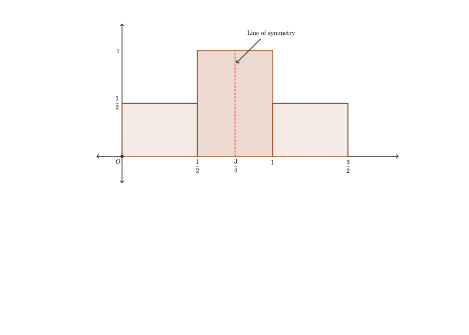
Figure 1. Density function $f$ for the nonuniform probability distribution $P$.

Proposition 3.2.

The optimal set of two-means is $\{\frac{7}{16},\frac{17}{16}\}$ with quantization error $V_{2}=\frac{37}{768}$.

Proof.

Let $\alpha:=\{a_{1},a_{2}\}$ be an optimal set of two means. Since the points in an optimal set are the conditional expectations in their own Voronoi region, we can assume that $0<a_{1}<a_{2}<\frac{3}{2}$. Again, due to symmetry of the probability distribution $P$ about the point $\frac{3}{4}$, we can assume that the boundary $\frac{1}{2}(a_{1}+a_{2})$ of the Voronoi regions of $a_{1}$ and $a_{2}$ passes through the midpoint $\frac{3}{4}$ of the support of $P$. Thus, we have

$$a_{1}=E(X:X\in[0,\frac{3}{4}])=\frac{\frac{1}{2}\int_{0}^{\frac{1}{2}}x\,dx+\int_{\frac{1}{2}}^{\frac{3}{4}}x\,dx}{\frac{1}{2}\int_{0}^{\frac{1}{2}}1\,dx+\int_{\frac{1}{2}}^{\frac{3}{4}}1\,dx}=\frac{7}{16},$$

and since $\frac{1}{2}(a_{1}+a_{2})=\frac{3}{4}$, we have $a_{2}=\frac{17}{16}$. Again, due to symmetry, the quantization error for two-means is given by

$$V_{2}=2\Big{(}\frac{1}{2}\int_{0}^{\frac{1}{2}}(x-\frac{7}{16})^{2}\,dx+\int_{\frac{1}{2}}^{\frac{3}{4}}(x-\frac{7}{16})^{2}\,dx\Big{)}=\frac{37}{768}.$$

Thus the proof of the proposition is complete (also see Figure 2). ∎

Proposition 3.3.

The optimal set of three-means is $\{\frac{1}{4},\frac{3}{4},\frac{5}{4}\}$ with quantization error $V_{3}=\frac{1}{48}$.

Proof.

Let $\alpha$ be an optimal set of three-means. As mentioned in Remark 3.1, we can assume that $\frac{3}{4}\in\alpha$. Let the other two elements in $\alpha$ be $a_{1}$ and $a_{2}$ such that $0<a_{1}<\frac{3}{4}<a_{2}<\frac{3}{2}$. Now, the boundary of the Voronoi regions of $a_{1}$ and $\frac{3}{4}$ is $\frac{1}{2}(a_{1}+\frac{3}{4})$. The following two cases can arise:

Case 1. $\frac{1}{2}(a_{1}+\frac{3}{4})\leq\frac{1}{2}.$

In this case, due to symmetry the distortion error is given by

$$\int\min_{a\in\alpha}(x-a)^{2}dP=2\Big{(}\frac{1}{2}\int_{0}^{\frac{1}{2}(a_{1}+\frac{3}{4})}(x-a_{1}){}^{2}\,dx+\frac{1}{2}\int_{\frac{1}{2}(a_{1}+\frac{3}{4})}^{\frac{1}{2}}(x-\frac{3}{4})^{2}\,dx+\int_{\frac{1}{2}}^{\frac{3}{4}}(x-\frac{3}{4})^{2}\,dx\Big{)}$$

$$=\frac{1}{768}\Big{(}192a_{1}^{3}+144a_{1}^{2}-108a_{1}+31\Big{)},$$

the minimum value of which is $0.0208333$ and it occurs when $a_{1}=\frac{1}{4}$.

Case 2. $\frac{1}{2}\leq\frac{1}{2}(a_{1}+\frac{3}{4}).$

In this case, due to symmetry the distortion error is given by

$$\int\min_{a\in\alpha}(x-a)^{2}dP=2\Big{(}\frac{1}{2}\int_{0}^{\frac{1}{2}}(x-a_{1}){}^{2}\,dx+\int_{\frac{1}{2}}^{\frac{1}{2}(a_{1}+\frac{3}{4})}(x-a_{1}){}^{2}\,dx+\int_{\frac{1}{2}(a_{1}+\frac{3}{4})}^{\frac{3}{4}}(x-\frac{3}{4})^{2}\,dx\Big{)}$$

$$=\frac{1}{384}\Big{(}192a_{1}^{3}-48a_{1}^{2}-12a_{1}+11\Big{)},$$

the minimum value of which is $0.0208333$ and it occurs when $a_{1}=\frac{1}{4}$.

Thus, considering all the possible cases we see that the distortion error is smallest when $a_{1}=\frac{1}{4}$, and since $\frac{1}{2}(a_{1}+a_{2})=\frac{3}{4}$, we have $a_{2}=\frac{5}{4}$. Thus, the optimal set of three-means is $\{\frac{1}{4},\frac{3}{4},\frac{5}{4}\}$ with quantization error $V_{3}=\frac{1}{48}$ (also see Figure 2). ∎

Proposition 3.4.

The optimal set of four-means is $\{0.198223,0.59467,0.90533,1.30178\}$ with quantization error $V_{4}=0.01057$.

Proof.

Let $\alpha:=\{a_{1},a_{2},a_{3},a_{4}\}$ be an optimal set of four-means. Due to symmetry of the probability measure we can say that the points in the optimal set will be symmetrically located on the line with respect to the point $\frac{3}{4}$, i.e., $0<a_{1}<a_{2}<\frac{3}{4}<a_{3}<a_{4}<\frac{3}{2}$, and $\frac{3}{4}$ is the midpoint of $a_{2}$ and $a_{3}$. The following cases can arise:

Case 1. $0<a_{1}<a_{2}\leq\frac{1}{2}$.

In this case, due to symmetry the distortion error is given by

$$\int\min_{a\in\alpha}(x-a)^{2}dP=2\Big{(}\frac{1}{2}\int_{0}^{\frac{1}{2}(a_{1}+a_{2})}(x-a_{1}){}^{2}\,dx+\int_{\frac{1}{2}}^{\frac{3}{4}}(x-a_{2}){}^{2}\,dx+\frac{1}{2}\int_{\frac{1}{2}(a_{1}+a_{2})}^{\frac{1}{2}}(x-a_{2}){}^{2}\,dx\Big{)}$$

$$=\frac{1}{96}\Big{(}24a_{1}^{3}+24a_{2}a_{1}^{2}-24a_{2}^{2}a_{1}-24a_{2}^{3}+96a_{2}^{2}-84a_{2}+23\Big{)},$$

the minimum value of which is $0.0150463$ and it occurs when $a_{1}=0.166667$ and $a_{2}=0.5$.

Case 2. $0<a_{1}\leq\frac{1}{2}<a_{2}<\frac{3}{4}$.

In this case, the following two subcases can occur.

Subcase 1. $\frac{1}{2}(a_{1}+a_{2})\leq\frac{1}{2}.$

In this subcase, due to symmetry the distortion error is given by

$$\int\min_{a\in\alpha}(x-a)^{2}dP=2\Big{(}\frac{1}{2}\int_{0}^{\frac{1}{2}(a_{1}+a_{2})}(x-a_{1}){}^{2}\,dx+\int_{\frac{1}{2}}^{\frac{3}{4}}(x-a_{2}){}^{2}\,dx+\frac{1}{2}\int_{\frac{1}{2}(a_{1}+a_{2})}^{\frac{1}{2}}(x-a_{2}){}^{2}\,dx\Big{)}$$

$$=\frac{1}{96}\Big{(}24a_{1}^{3}+24a_{2}a_{1}^{2}-24a_{2}^{2}a_{1}-24a_{2}^{3}+96a_{2}^{2}-84a_{2}+23\Big{)},$$

the minimum value of which is $0.01057$ and it occurs when $a_{1}=0.198223$ and $a_{2}=0.59467$.

Subcase 2. $\frac{1}{2}\leq\frac{1}{2}(a_{1}+a_{2}).$

In this case, due to symmetry the distortion error is given by

$$\int\min_{a\in\alpha}(x-a)^{2}dP=2\Big{(}\frac{1}{2}\int_{0}^{\frac{1}{2}}(x-a_{1}){}^{2}\,dx+\int_{\frac{1}{2}}^{\frac{1}{2}(a_{1}+a_{2})}(x-a_{1}){}^{2}\,dx+\int_{\frac{1}{2}(a_{1}+a_{2})}^{\frac{3}{4}}(x-a_{2}){}^{2}\,dx\Big{)}$$

$$=\frac{1}{96}(48a_{1}^{3}+48(a_{2}-1)a_{1}^{2}+(24-48a_{2}^{2})a_{1}-48a_{2}^{3}+144a_{2}^{2}-108a_{2}+23),$$

the minimum value of which is $0.0169271$ and it occurs when $a_{1}=0.3125$ and $a_{2}=0.6875$.

Case 3. $\frac{1}{2}\leq a_{1}<a_{2}<\frac{3}{4}$.

Notice that in this case we obtain

$$\int\min_{a\in\alpha}(x-a)^{2}dP\geq\frac{2}{2}\int_{0}^{\frac{1}{2}}(x-\frac{1}{2})^{2}\,dx=\frac{1}{24}=0.0416667,$$

which is larger than the distortion errors obtained in at least one of the previous cases. So, this case cannot happen.

Thus, considering all the possible cases, we can deduce that the smallest distortion error is $V_{4}=0.01057$, and it occurs when $a_{1}=0.198223$ and $a_{2}=0.59467$. Since $\frac{1}{2}(a_{2}+a_{3})=\frac{3}{4}$ and $\frac{1}{2}(a_{1}+a_{4})=\frac{3}{4}$, we have $a_{3}=0.90533$ and $a_{4}=1.30178$. Thus, the optimal set of four-means is $\{0.198223,0.59467,0.90533,1.30178\}$ with quantization error $V_{4}=0.01057$, which is the proposition (also see Figure 2). ∎

Proposition 3.5.

The optimal set of five-means is $\{0.169821,0.509464,\frac{3}{4},0.990536,1.33018\}$ with quantization error $V_{5}=0.00721728$.

Proof.

Let $\alpha:=\{a_{1}<a_{2}<a_{3}<a_{4}<a_{5}\}$ be an optimal set of five-means. As mentioned in Remark 3.1, we can assume that $a_{3}=\frac{3}{4}$. The following cases can happen.

Case 1. $a_{2}\leq\frac{1}{2}$

In this case the following subcases can happen.

Subcase 1. $\frac{1}{2}(a_{2}+\frac{3}{4})\leq\frac{1}{2}$.

Due to symmetry the distortion error is given by

$$\int\min_{a\in\alpha}(x-a)^{2}dP =2\Big{(}\frac{1}{2}\int_{0}^{\frac{1}{2}(a_{1}+a_{2})}(x-a_{1}){}^{2}\,dx+\frac{1}{2}\int_{\frac{1}{2}(a_{2}+\frac{3}{4})}^{\frac{1}{2}}(x-\frac{3}{4})^{2}\,dx+\frac{1}{2}\int_{\frac{1}{2}(a_{1}+a_{2})}^{\frac{1}{2}(a_{2}+\frac{3}{4})}(x-a_{2}){}^{2}\,dx$$

$$\qquad\qquad\qquad+\int_{\frac{1}{2}}^{\frac{3}{4}}(x-\frac{3}{4})^{2}\,dx\Big{)}$$

$$=\frac{1}{768}\Big{(}192a_{1}^{3}+192a_{2}a_{1}^{2}-192a_{2}^{2}a_{1}+144a_{2}^{2}-108a_{2}+31\Big{)},$$

the minimum value of which is $0.0162037$, and it occurs when $a_{1}=0.0833333$ and $a_{2}=0.25$.

Subcase 2. $\frac{1}{2}\leq\frac{1}{2}(a_{2}+\frac{3}{4})$.

Due to symmetry the distortion error is given by

$$\int\min_{a\in\alpha}(x-a)^{2}dP =2\Big{(}\frac{1}{2}\int_{0}^{\frac{1}{2}(a_{1}+a_{2})}(x-a_{1}){}^{2}\,dx+\int_{\frac{1}{2}(a_{2}+\frac{3}{4})}^{\frac{3}{4}}(x-\frac{3}{4})^{2}\,dx+\int_{\frac{1}{2}}^{\frac{1}{2}(a_{2}+\frac{3}{4})}(x-a_{2}){}^{2}\,dx$$

$$\qquad\qquad\qquad+\frac{1}{2}\int_{\frac{1}{2}(a_{1}+a_{2})}^{\frac{1}{2}}(x-a_{2}){}^{2}\,dx\Big{)}$$

$$=\frac{1}{384}\Big{(}96a_{1}^{3}+96a_{2}a_{1}^{2}-96a_{2}^{2}a_{1}+96a_{2}^{3}-48a_{2}^{2}-12a_{2}+11\Big{)},$$

the minimum value of which is $0.0162037$, and it occurs when $a_{1}=0.0833333$ and $a_{2}=0.25$.

Case 2. $0<a_{1}\leq\frac{1}{2}<a_{2}<\frac{3}{4}$.

In this case the following subcases can happen.

Subcase 1. $\frac{1}{2}(a_{1}+a_{2})\leq\frac{1}{2}$.

Due to symmetry the distortion error is given by

$$\int\min_{a\in\alpha}(x-a)^{2}dP =2\Big{(}\int_{\frac{1}{2}(a_{2}+\frac{3}{4})}^{\frac{3}{4}}(x-\frac{3}{4})^{2}\,dx+\frac{1}{2}\int_{0}^{\frac{1}{2}(a_{1}+a_{2})}(x-a_{1}){}^{2}\,dx+\int_{\frac{1}{2}}^{\frac{1}{2}(a_{2}+\frac{3}{4})}(x-a_{2}){}^{2}\,dx$$

$$\qquad\qquad\qquad+\frac{1}{2}\int_{\frac{1}{2}(a_{1}+a_{2})}^{\frac{1}{2}}(x-a_{2}){}^{2}\,dx\Big{)}$$

$$=\frac{1}{384}\Big{(}96a_{1}^{3}+96a_{2}a_{1}^{2}-96a_{2}^{2}a_{1}+96a_{2}^{3}-48a_{2}^{2}-12a_{2}+11\Big{)},$$

the minimum value of which is $0.00721728$, and it occurs when $a_{1}=0.169821$ and $a_{2}=0.509464$.

Subcase 2. $\frac{1}{2}\leq\frac{1}{2}(a_{1}+a_{2})$.

Due to symmetry the distortion error is given by

$$\int\min_{a\in\alpha}(x-a)^{2}dP =2\Big{(}\int_{\frac{1}{2}(a_{2}+\frac{3}{4})}^{\frac{3}{4}}(x-\frac{3}{4})^{2}\,dx+\frac{1}{2}\int_{0}^{\frac{1}{2}}(x-a_{1}){}^{2}\,dx+\int_{\frac{1}{2}}^{\frac{1}{2}(a_{1}+a_{2})}(x-a_{1}){}^{2}\,dx$$

$$\qquad\qquad\qquad+\int_{\frac{1}{2}(a_{1}+a_{2})}^{\frac{1}{2}(a_{2}+\frac{3}{4})}(x-a_{2}){}^{2}\,dx\Big{)}$$

$$=\frac{1}{384}\Big{(}192a_{1}^{3}+192(a_{2}-1)a_{1}^{2}-96(2a_{2}^{2}-1)a_{1}+144a_{2}^{2}-108a_{2}+11\Big{)},$$

the minimum value of which is $0.0167955$, and it occurs when $a_{1}=0.315741$ and $a_{2}=0.684259$.

Case 3. $\frac{1}{2}<a_{1}<a_{2}<\frac{3}{4}$.

Due to symmetry the distortion error is given by

$$\int\min_{a\in\alpha}(x-a)^{2}dP>2\times\frac{1}{2}\int_{0}^{\frac{1}{2}}(x-\frac{1}{2})^{2}\,dx=0.0416667$$

which is larger than the distortion error that arises in at least one of the previous cases.

Taking into consideration all the above possible cases, we see that the quantization error for optimal set of five-means is $V_{5}=0.00721728$, and it occurs when $a_{1}=0.169821$ and $a_{2}=0.509464$. Due to symmetry, we have $a_{4}=0.990536$ and $a_{5}=1.33018$. Thus, the proof of the proposition is complete (also see Figure 2). ∎

Let us now prove the following lemma.

Lemma 3.6.

Let $\alpha_{n}$ be an optimal set of $n$-means for $n\geq 4$. Then, $\alpha_{n}$ contains points from both the open intervals $(0,\frac{1}{2})$ and $(\frac{1}{2},\frac{3}{4})$.

Proof.

By Propositions 3.4 and Proposition 3.5, the lemma is true for $n=4$ and $n=5$. Let us now prove the lemma for $n\geq 6$. We prove it by contradiction. Recall Remark 3.1, and also recall that for $n\geq 6$, we have $V_{n}\leq V_{6}<V_{5}$. For $n\geq 6$, if $\alpha_{n}$ does not contain any point from the open interval $(\frac{1}{2},\frac{3}{4})$, then due to symmetry we have

$$V_{n}\geq 2\int_{\frac{1}{2}}^{\frac{3}{4}}(x-\frac{1}{2})^{2}\,dx=\frac{1}{96}=0.0104167>V_{5},$$

which leads to a contradiction. For $n\geq 6$, if $\alpha_{n}$ does not contain any point from the open interval $(0,\frac{1}{2})$, then due to symmetry we have

$$V_{n}\geq\frac{2}{2}\int_{0}^{\frac{1}{2}}(x-\frac{1}{2})^{2}\,dx=\frac{1}{24}=0.0416667>V_{5},$$

which is a contradiction. Hence, we can conclude that the lemma is also true for $n\geq 6$. Thus, the proof of the lemma is complete. ∎

Proposition 3.7.

The optimal set of six-means is $\{0.125,0.375,0.625,0.875,1.125,1.375\}$ with quantization error $V_{6}=0.00520833$.

Proof.

Let $\alpha:=\{a_{1},a_{2},a_{3},a_{4},a_{5},a_{6}\}$ be an optimal set of six-means. Due to symmetry of the probability measure we can say that the points in the optimal set will be symmetrically located on the line with respect to the point $\frac{3}{4}$, i.e., $0<a_{1}<a_{2}<a_{3}<\frac{3}{4}<a_{4}<a_{5}<a_{6}<\frac{3}{2}$, and $\frac{3}{4}$ is the midpoint of $a_{2}$ and $a_{3}$. By Lemma 3.6, we can say that $a_{1}<\frac{1}{2}$, and $\frac{1}{2}<a_{3}$.

The following cases can arise:

Case 1. $0<a_{1}<a_{2}\leq\frac{1}{2}$.

The following two subcases can occur.

Subcase 1. $0<a_{1}<a_{2}<\frac{1}{2}(a_{2}+a_{3})\leq\frac{1}{2}<a_{3}<\frac{3}{4}$.

In this subcase, due to symmetry the distortion error is given by

$$\int\min_{a\in\alpha}(x-a)^{2}dP=2\Big{(}\frac{1}{2}\int_{0}^{\frac{1}{2}(a_{1}+a_{2})}(x-a_{1}){}^{2}\,dx+\frac{1}{2}\int_{\frac{1}{2}(a_{1}+a_{2})}^{\frac{1}{2}(a_{2}+a_{3})}(x-a_{2}){}^{2}\,dx+\int_{\frac{1}{2}}^{\frac{3}{4}}(x-a_{3}){}^{2}\,dx$$

$$\qquad\qquad\qquad+\frac{1}{2}\int_{\frac{1}{2}(a_{2}+a_{3})}^{\frac{1}{2}}(x-a_{3}){}^{2}\,dx\Big{)}$$

$$=\frac{1}{96}\Big{(}24a_{1}^{3}+24a_{2}a_{1}^{2}-24a_{2}^{2}a_{1}-24a_{3}^{3}-24(a_{2}-4)a_{3}^{2}+12(2a_{2}^{2}-7)a_{3}+23\Big{)},$$

the minimum value of which is $0.00520833$ and it occurs when $a_{1}=0.125$, $a_{2}=0.375$ and $a_{3}=0.625$.

Subcase 2. $0<a_{1}<a_{2}<\frac{1}{2}\leq\frac{1}{2}(a_{2}+a_{3})<a_{3}<\frac{3}{4}$.

In this subcase, due to symmetry the distortion error is given by

$$\int\min_{a\in\alpha}(x-a)^{2}dP=2\Big{(}\frac{1}{2}\int_{0}^{\frac{1}{2}(a_{1}+a_{2})}(x-a_{1}){}^{2}\,dx+\int_{\frac{1}{2}}^{\frac{1}{2}(a_{2}+a_{3})}(x-a_{2}){}^{2}\,dx+\frac{1}{2}\int_{\frac{1}{2}(a_{1}+a_{2})}^{\frac{1}{2}}(x-a_{2}){}^{2}\,dx$$

$$\qquad\qquad\qquad+\int_{\frac{1}{2}(a_{2}+a_{3})}^{\frac{3}{4}}(x-a_{3}){}^{2}\,dx\Big{)}$$

$$=\frac{1}{96}\Big{(}24a_{1}^{3}+24a_{2}a_{1}^{2}-24a_{2}^{2}a_{1}+24a_{2}^{3}-48a_{3}^{3}+144a_{3}^{2}+48a_{2}^{2}(a_{3}-1)-108a_{3}+a_{2}(24-48a_{3}^{2})+23\Big{)},$$

the minimum value of which is $0.00520833$ and it occurs when $a_{1}=0.125$, $a_{2}=0.375$ and $a_{3}=0.625$.

Case 2. $0<a_{1}<\frac{1}{2}<a_{2}<a_{3}<\frac{3}{4}$.

In this case, proceeding as before considering the two subcases: $\frac{1}{2}\left(a_{1}+a_{2}\right)\leq\frac{1}{2}<a_{2}<a_{3}<\frac{3}{4}$, and $\frac{1}{2}\leq\frac{1}{2}\left(a_{1}+a_{2}\right)<a_{2}<a_{3}<\frac{3}{4}$, it can be shown that the distortion error is larger than the distortion error obtained in Case 1. Therefore, this case cannot happen.

Hence, the quantization error for six-means is $V_{6}=0.00520833$, and it occurs when $a_{1}=0.125,\,a_{2}=0.375,\,a_{3}=0.625$. Due to symmetry, we have $a_{4}=0.875,\,a_{5}=1.125$, and $a_{6}=1.375$. Thus, the proof of the proposition is complete (also see Figure 2). ∎

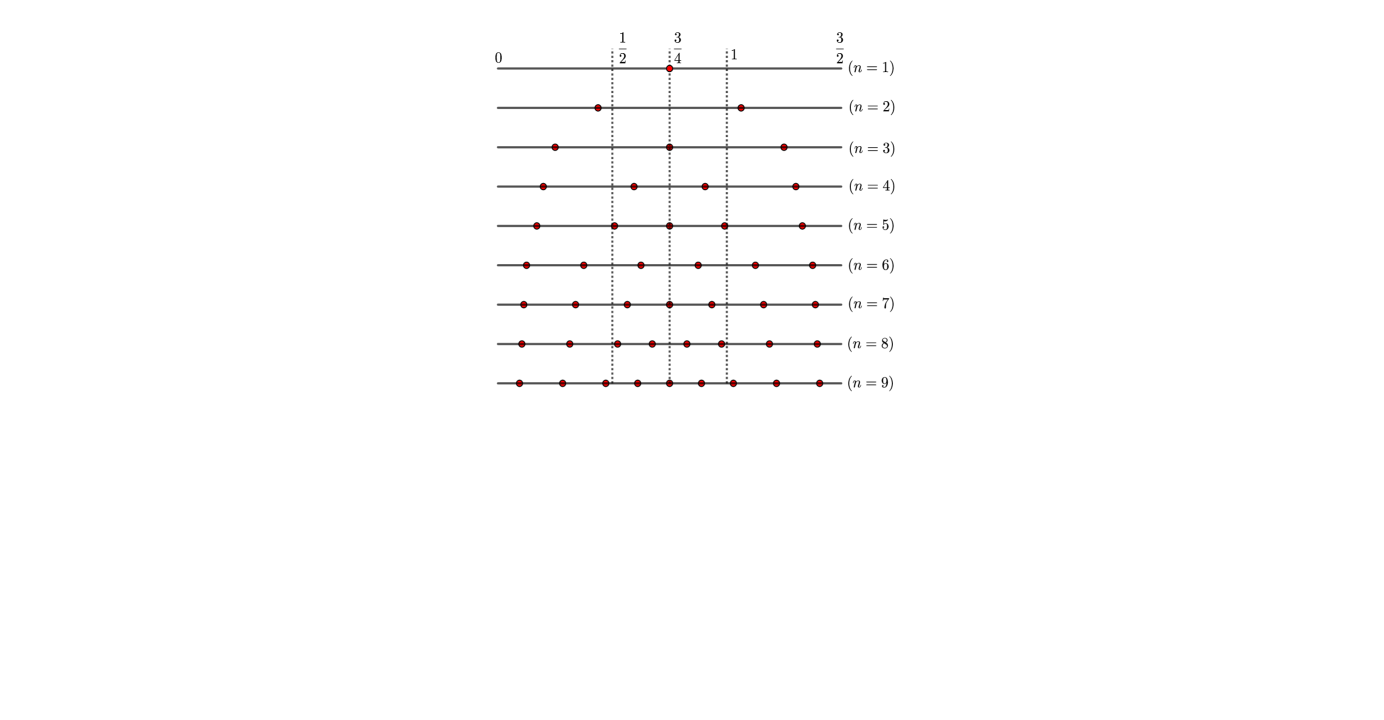
Figure 2. Points in the optimal sets of $n$-means for $1\leq n\leq 9$.

In the following section we calculate the optimal sets of $n$-means and the $n$th quantization errors for all $n\geq 5$.

4. Optimal sets of $n$-means and the $n$th quantization errors for all $n\geq 5$

Let $n\geq 5$ be a positive integer. By Remark 3.1, we know that if $n$ is odd, an optimal set $\alpha_{n}$ of $n$-means always contains the point $\frac{3}{4}$. Notice that whether $n$ is an even or an odd positive integer, it is enough to find the elements in an optimal set which are to the left side of $\frac{3}{4}$, i.e., which are belonged to the interval $(0,\frac{3}{4})$; the remaining elements in $\alpha_{n}$ can be obtained by taking the reflections with respect to the point $\frac{3}{4}$. By Lemma 3.6, an optimal set $\alpha_{n}$ contains points from both the open intervals $(0,\frac{1}{2})$ and $(\frac{1}{2},\frac{3}{4})$. Thus, there exist two positive integers $k:=k(n)$ and $m:=m(n)$ such that

$$\alpha_{n}\cap[0,\frac{1}{2}] :=\{a_{1}<a_{2}<\cdots<a_{k}\},\text{ and }$$

$$\alpha_{n}\cap(\frac{1}{2},\frac{3}{4}] :=\left\{\begin{array}[]{cc}\{b_{1}<b_{2}<\cdots<b_{m}\}&\text{ if $n$ is even,}\\ \{b_{1}<b_{2}<\cdots<b_{m}<\frac{3}{4}\}&\text{ if $n$ is odd.}\end{array}\right.$$

Observe that in the above expression, if $n$ is even, then $2(k+m)=n$; and if $n$ is odd, then $2(k+m)+1=n$. Notice that the following two cases can happen: either $\frac{1}{2}(a_{k}+b_{1})\leq\frac{1}{2}$, or $\frac{1}{2}\leq\frac{1}{2}(a_{k}+b_{1})$. Whether $n$ is even or odd, let $V1(k,m)$ be the $n$th quantization error when $\frac{a_{k}+b_{1}}{2}\leq\frac{1}{2}$, and $V2(k,m)$ be the $n$th quantization error when $\frac{1}{2}\leq\frac{a_{k}+b_{1}}{2}$. The optimal sets of $n$-means and the $n$th quantization errors for $n=1,2,3,4,5$ are given in the previous sections. The following propositions will give the optimal sets of $n$-means and the $n$th quantization errors for all $n\geq 6$.

Proposition 4.1.

Let $k\geq 2$ and $m=1$. Then, if $\frac{1}{2}(a_{k}+b_{1})\leq\frac{1}{2}$, we have $a_{j}=\frac{(2j-1)(a_{k}+b_{1})}{4k}$ for $1\leq j\leq k$, and

$$b_{1}=\left\{\begin{array}[]{cc}E(X:X\in[\frac{1}{2}(a_{k}+b_{1}),\frac{3}{4}])&\text{ if $n$ is even},\\ E(X:X\in[\frac{1}{2}(a_{k}+b_{1}),\frac{1}{2}(b_{1}+\frac{3}{4})])&\text{ if $n$ is odd};\end{array}\right.$$

and if $\frac{1}{2}\leq\frac{1}{2}(a_{k}+b_{1})$, we have $a_{j}=\frac{(2j-1)(a_{k-1}+a_{k})}{4(k-1)}$ for $1\leq j\leq(k-1)$, $a_{k}=E(X:X\in[\frac{1}{2}(a_{k-1}+a_{k}),\frac{1}{2}(a_{k}+b_{1})])$, and

$$b_{1}=\left\{\begin{array}[]{cc}E(X:X\in[\frac{1}{2}(a_{k}+b_{1}),\frac{3}{4}])&\text{ if $n$ is even},\\ E(X:X\in[\frac{1}{2}(a_{k}+b_{1}),\frac{1}{2}(b_{1}+\frac{3}{4})])&\text{ if $n$ is odd}.\end{array}\right.$$

The quantization errors for $n$-means are given by

$$V1(k,1)=\left\{\begin{array}[]{cc}2\Big{(}\frac{(a_{k}+b_{1}){}^{3}}{192k^{2}}+\frac{1}{2}\int_{\frac{1}{2}(a_{k}+b_{1})}^{\frac{1}{2}}(x-b_{1}){}^{2}\,dx+\int_{\frac{1}{2}}^{\frac{3}{4}}(x-b_{1}){}^{2}\,dx\Big{)}&\text{ if $n$ is even},\\ 2\Big{(}\frac{(a_{k}+b_{1}){}^{3}}{192k^{2}}+\frac{1}{2}\int_{\frac{1}{2}(a_{k}+b_{1})}^{\frac{1}{2}}(x-b_{1}){}^{2}\,dx+\int_{\frac{1}{2}}^{\frac{1}{2}(b_{1}+\frac{3}{4})}(x-b_{1}){}^{2}\,dx\\ +\int_{\frac{1}{2}(b_{1}+\frac{3}{4})}^{\frac{3}{4}}(x-\frac{3}{4})^{2}\,dx\Big{)}&\text{ if $n$ is odd};\end{array}\right.$$

and

$$V2(k,1)=\left\{\begin{array}[]{cc}2\Big{(}\frac{(a_{k-1}+a_{k}){}^{3}}{192(k-1)^{2}}+\frac{1}{2}\int_{\frac{1}{2}(a_{k-1}+a_{k})}^{\frac{1}{2}}(x-a_{k}){}^{2}\,dx+\int_{\frac{1}{2}}^{\frac{1}{2}(a_{k}+b_{1})}(x-a_{k}){}^{2}\,dx\\ +\int_{\frac{1}{2}(a_{k}+b_{1})}^{\frac{3}{4}}(x-b_{1}){}^{2}\,dx\Big{)}&\text{ if $n$ is even},\\ 2\Big{(}\frac{(a_{k-1}+a_{k}){}^{3}}{192(k-1)^{2}}+\frac{1}{2}\int_{\frac{1}{2}(a_{k-1}+a_{k})}^{\frac{1}{2}}(x-a_{k}){}^{2}\,dx+\int_{\frac{1}{2}}^{\frac{1}{2}(a_{k}+b_{1})}(x-a_{k}){}^{2}\,dx\\ +\int_{\frac{1}{2}(a_{k}+b_{1})}^{\frac{1}{2}(b_{1}+\frac{3}{4})}(x-b_{1}){}^{2}\,dx+\int_{\frac{1}{2}(b_{1}+\frac{3}{4})}^{\frac{3}{4}}(x-\frac{3}{4})^{2}\,dx\Big{)}&\text{ if $n$ is odd}.\end{array}\right.$$

Proof.

If $\frac{a_{k}+b_{1}}{2}\leq\frac{1}{2}$, then $a_{1},a_{2},\cdots,a_{k}$ are uniformly distributed over the closed interval $[0,\frac{a_{k}+b_{1}}{2}]$; on the other hand, if $\frac{1}{2}\leq\frac{a_{k}+b_{1}}{2}$, then $a_{1},a_{2},\cdots,a_{k-1}$ are uniformly distributed over the closed interval $[0,\frac{a_{k-1}+a_{k}}{2}]$. Thus, by Proposition 2.3 and Proposition 1.1, the expressions for $a_{j}$ and $b_{j}$ can be obtained. With the help of the formula given in Proposition 2.3, the quantization errors are also obtained as routine. ∎

Proposition 4.2.

Let $k=1$ and $m\geq 2$. Then, if $\frac{1}{2}(a_{1}+b_{1})\leq\frac{1}{2}$, we have $a_{1}=E(X:X\in[0,\frac{1}{2}(a_{1}+b_{1})]$, $b_{1}=E(X:X\in[\frac{1}{2}(a_{1}+b_{1}),\frac{1}{2}(b_{1}+b_{2})])$, and

$$b_{1+j}=\left\{\begin{array}[]{cc}\frac{1}{2}(b_{1}+b_{2})+\frac{(2j-1)}{2(m-1)}(\frac{3}{4}-\frac{1}{2}(b_{1}+b_{2}))\text{ for }1\leq j\leq m-1&\text{ if $n$ is even},\\ \frac{1}{2}(b_{1}+b_{2})+\frac{(2j-1)}{2(m-1)}(\frac{3}{4}-b_{2})\text{ for }1\leq j\leq m-1&\text{ if $n$ is odd};\end{array}\right.$$

and if $\frac{1}{2}\leq\frac{1}{2}(a_{1}+b_{1})$, we have $a_{1}=E(X:X\in[0,\frac{1}{2}(a_{1}+b_{1})]$, and

$$b_{j}=\left\{\begin{array}[]{cc}\frac{1}{2}(a_{1}+b_{1})+\frac{(2j-1)}{2m}(\frac{3}{4}-\frac{1}{2}(a_{1}+b_{1}))$ for $1\leq j\leq m&\text{ if $n$ is even},\\ \frac{1}{2}(a_{1}+b_{1})+\frac{(2j-1)}{2m}(\frac{3}{4}-b_{1})\text{ for }1\leq j\leq m&\text{ if $n$ is odd};\end{array}\right.$$

The quantization errors for $n$-means are given by

$$V1(1,m)=\left\{\begin{array}[]{cc}2\Big{(}\frac{1}{2}\int_{0}^{\frac{1}{2}(a_{1}+b_{1})}(x-a_{1}){}^{2}\,dx+\frac{1}{2}\int_{\frac{1}{2}(a_{1}+b_{1})}^{\frac{1}{2}}(x-b_{1}){}^{2}\,dx\\ +\int_{\frac{1}{2}}^{\frac{1}{2}(b_{1}+b_{2})}(x-b_{1}){}^{2}\,dx+\frac{(3-2(b_{1}+b_{2}))^{3}}{768(m-1)^{2}}\Big{)}&\text{ if $n$ is even},\\ 2\Big{(}\frac{1}{2}\int_{0}^{\frac{1}{2}(a_{1}+b_{1})}(x-a_{1}){}^{2}\,dx+\frac{1}{2}\int_{\frac{1}{2}(a_{1}+b_{1})}^{\frac{1}{2}}(x-b_{1}){}^{2}\,dx\\ +\int_{\frac{1}{2}}^{\frac{1}{2}(b_{1}+b_{2})}(x-b_{1}){}^{2}\,dx+\frac{(3-4b_{2}){}^{3}}{768(m-1)^{2}}+\frac{1}{24}(b_{2}-b_{1}){}^{3}\Big{)}&\text{ if $n$ is odd};\end{array}\right.$$

and

$$V2(1,m)=\left\{\begin{array}[]{cc}2\Big{(}\frac{1}{2}\int_{0}^{\frac{1}{2}}\left(x-a_{1}\right){}^{2}\,dx+\int_{\frac{1}{2}}^{\frac{1}{2}\left(a_{1}+b_{1}\right)}\left(x-a_{1}\right){}^{2}\,dx+\frac{\left(3-2(a_{1}+b_{1})\right){}^{3}}{768m^{2}}\Big{)}&\text{ if $n$ is even},\\ 2\Big{(}\frac{1}{2}\int_{0}^{\frac{1}{2}}\left(x-a_{1}\right){}^{2}\,dx+\int_{\frac{1}{2}}^{\frac{1}{2}\left(a_{1}+b_{1}\right)}\left(x-a_{1}\right){}^{2}\,dx\\ +\frac{(3-4b_{1}){}^{3}}{768m^{2}}+\frac{1}{24}(b_{1}-a_{1}){}^{3}\Big{)}&\text{ if $n$ is odd}.\end{array}\right.$$

Proof.

If $\frac{1}{2}(a_{1}+b_{1})\leq\frac{1}{2}$ and $n$ is even, then $b_{2},b_{3},\cdots,b_{m}$ are uniformly distributed over the closed interval $[\frac{1}{2}(b_{1}+b_{2}),\frac{3}{4}]$, and so by Proposition 2.3, the expressions for $b_{i+j}$, where $1\leq j\leq(m-1)$, and the corresponding quantization error can be obtained. On the other hand, if $\frac{1}{2}(a_{1}+b_{1})\leq\frac{1}{2}$ and $n$ is odd, then as $\{b_{2}<b_{3}<\cdots<b_{m}<\frac{3}{4}\}$ is the set of optimal quantizers with respect to the probability distribution $P(\cdot|_{[\frac{1}{2}(b_{1}+b_{2}),\frac{3}{4}]})$ with constant density $f(x)=1$ for all $x\in[\frac{1}{2}(b_{1}+b_{2}),\frac{3}{4}]$, the expressions for $b_{j}$, and the corresponding quantization error can be obtained using Proposition 2.4. Likewise, if $\frac{1}{2}\leq\frac{1}{2}(a_{1}+b_{1})$, using Proposition 2.3 and Proposition 2.4, we get the expressions for the optimal quantizers and the corresponding quantization error. ∎

Proposition 4.3.

Let $k\geq 2$ and $m\geq 2$. Then, if $\frac{1}{2}(a_{k}+b_{1})\leq\frac{1}{2}$, we have $a_{j}=\frac{(2j-1)(a_{k}+b_{1})}{4k}$ for $1\leq j\leq k$, $b_{1}=E(X:X\in[\frac{1}{2}(a_{k}+b_{1}),\frac{1}{2}(b_{1}+b_{2})])$, and

$$b_{1+j}=\left\{\begin{array}[]{cc}\frac{1}{2}(b_{1}+b_{2})+\frac{(2j-1)}{2(m-1)}(\frac{3}{4}-\frac{1}{2}(b_{1}+b_{2}))\text{ for }1\leq j\leq m-1&\text{ if $n$ is even},\\ \frac{1}{2}(b_{1}+b_{2})+\frac{(2j-1)}{2(m-1)}(\frac{3}{4}-b_{2})\text{ for }1\leq j\leq m-1&\text{ if $n$ is odd};\end{array}\right.$$

and if $\frac{1}{2}\leq\frac{1}{2}(a_{k}+b_{1})$, we have $a_{j}=\frac{(2j-1)(a_{k-1}+a_{k})}{4(k-1)}$ for $1\leq j\leq(k-1)$, $a_{k}=E(X:X\in[\frac{1}{2}(a_{k-1}+a_{k}),\frac{1}{2}(a_{k}+b_{1})])$, and

$$b_{j}=\left\{\begin{array}[]{cc}\frac{1}{2}(a_{k}+b_{1})+\frac{(2j-1)}{2m}(\frac{3}{4}-\frac{1}{2}(a_{k}+b_{1}))$ for $1\leq j\leq m&\text{ if $n$ is even},\\ \frac{1}{2}(a_{k}+b_{1})+\frac{(2j-1)}{2m}(\frac{3}{4}-b_{1})\text{ for }1\leq j\leq m&\text{ if $n$ is odd};\end{array}\right.$$

The quantization errors for $n$-means are given by

$$V1(k,m)=\left\{\begin{array}[]{cc}2\Big{(}\frac{(a_{k}+b_{1}){}^{3}}{192k^{2}}+\frac{1}{2}\int_{\frac{1}{2}(a_{k}+b_{1})}^{\frac{1}{2}}(x-b_{1}){}^{2}\,dx+\int_{\frac{1}{2}}^{\frac{1}{2}(b_{1}+b_{2})}(x-b_{1}){}^{2}\,dx\\ +\frac{(3-2(b_{1}+b_{2}))^{3}}{768(m-1)^{2}}\Big{)}&\text{ if $n$ is even},\\ 2\Big{(}\frac{(a_{k}+b_{1}){}^{3}}{192k^{2}}+\frac{1}{2}\int_{\frac{1}{2}(a_{k}+b_{1})}^{\frac{1}{2}}(x-b_{1}){}^{2}\,dx\\ +\int_{\frac{1}{2}}^{\frac{1}{2}(b_{1}+b_{2})}(x-b_{1}){}^{2}\,dx+\frac{(3-4b_{2}){}^{3}}{768(m-1)^{2}}+\frac{1}{24}(b_{2}-b_{1}){}^{3}\Big{)}&\text{ if $n$ is odd};\end{array}\right.$$

and

$$V2(k,m)=\left\{\begin{array}[]{cc}2\Big{(}\frac{(a_{k-1}+a_{k}){}^{3}}{192(k-1)^{2}}+\frac{1}{2}\int_{\frac{1}{2}(a_{k-1}+a_{k})}^{\frac{1}{2}}(x-a_{k}){}^{2}\,dx+\int_{\frac{1}{2}}^{\frac{1}{2}(a_{k}+b_{1})}(x-a_{k}){}^{2}\,dx\\ +\frac{\left(3-2(a_{k}+b_{1})\right){}^{3}}{768m^{2}}\Big{)}&\text{ if $n$ is even},\\ 2\Big{(}\frac{(a_{k-1}+a_{k}){}^{3}}{192(k-1)^{2}}+\frac{1}{2}\int_{\frac{1}{2}(a_{k-1}+a_{k})}^{\frac{1}{2}}(x-a_{k}){}^{2}\,dx+\int_{\frac{1}{2}}^{\frac{1}{2}(a_{k}+b_{1})}(x-a_{k}){}^{2}\,dx\\ +\frac{(3-4b_{1}){}^{3}}{768m^{2}}+\frac{1}{24}(b_{1}-a_{k}){}^{3}\Big{)}&\text{ if $n$ is odd}.\end{array}\right.$$

Proof.

Notice that Proposition 4.3 is a mixture of Proposition 4.1 and Proposition 4.2, and thus the proof follows in the similar lines. ∎

Lemma 4.4.

For any even positive integer $n\geq 4$, let $\alpha_{n}$ be an optimal set of $n$-means for $P$. Assume that $\text{card}(\alpha_{n}\cap[0,\frac{1}{2}])=k:=k(n)$ and $\text{card}(\alpha_{n}\cap(\frac{1}{2},\frac{3}{4}))=m:=m(n)$ for some positive integers $k$ and $m$. Then, either $\text{card}(\alpha_{n+2}\cap[0,\frac{1}{2}])=k+1$ and $\text{card}(\alpha_{n+2}\cap(\frac{1}{2},\frac{3}{4}))=m$, or $\text{card}(\alpha_{n+2}\cap[0,\frac{1}{2}])=k$ and $\text{card}(\alpha_{n+2}\cap(\frac{1}{2},\frac{3}{4}))=m+1$.

Proof.

For any even positive integer $n\geq 4$, let $\text{card}(\alpha_{n}\cap[0,\frac{1}{2}])=k:=k(n)$ and $\text{card}(\alpha_{n}\cap(\frac{1}{2},\frac{3}{4}))=m:=m(n)$ for some positive integers $k$ and $m$. Let $V(k(n),m(n))$ be the corresponding distortion error. By Proposition 3.4 and Proposition 3.7, we know that $\text{card}(\alpha_{4}\cap[0,\frac{1}{2}])=1$, $\text{card}(\alpha_{4}\cap(\frac{1}{2},\frac{3}{4}))=1$, $\text{card}(\alpha_{6}\cap[0,\frac{1}{2}])=2$, and $\text{card}(\alpha_{6}\cap(\frac{1}{2},\frac{3}{4}))=1$ Thus, the lemma is true for $n=4$. Let the lemma be true for $n=N$ for some even positive integer $N\geq 4$. Then, $\text{card}(\alpha_{N}\cap[0,\frac{1}{2}])=k(N)\text{ and }\text{card}(\alpha_{N}\cap(\frac{1}{2},\frac{3}{4}))=m(N)$ imply that either $\text{card}(\alpha_{N+2}\cap[0,\frac{1}{2}])=k(N)+1$ and $\text{card}(\alpha_{N+2}\cap(\frac{1}{2},\frac{3}{4}))=m(N)$, or $\text{card}(\alpha_{N+2}\cap[0,\frac{1}{2}])=k(N)$ and $\text{card}(\alpha_{N+2}\cap(\frac{1}{2},\frac{3}{4}))=m(N)+1$. Suppose that $\text{card}(\alpha_{N+2}\cap[0,\frac{1}{2}])=k(N)+1$ and $\text{card}(\alpha_{N+2}\cap(\frac{1}{2},\frac{3}{4}))=m(N)$ hold. Now, for the given $N$, by calculating the distortion errors $V(\ell,N+4-\ell)$ for all $1\leq\ell\leq N+3$, we see that the distortion error is smallest if $\text{card}(\alpha_{N+4}\cap[0,\frac{1}{2}])=k(N)+2\text{ and }\text{card}(\alpha_{N+2}\cap(\frac{1}{2},\frac{3}{4}))=m(N),\text{ or if }\text{card}(\alpha_{N+4}\cap[0,\frac{1}{2}])=k(N)+1\text{ and }\text{card}(\alpha_{N+4}\cap(\frac{1}{2},\frac{3}{4}))=m(N)+1$, i.e., the lemma is true for $n=N+2$ whenever it is true for $n=N$. Similarly, we can show that the lemma is true for $n=N+2$ if $\text{card}(\alpha_{N+2}\cap[0,\frac{1}{2}])=k(N)\text{ and }\text{card}(\alpha_{N+2}\cap(\frac{1}{2},\frac{3}{4}))=m(N)+1$ hold. Thus, by the induction principle, the proof of the lemma is complete. ∎

Proceeding in the similar lines as Lemma 4.4, the following lemma can be proved.

Lemma 4.5.

For any odd positive integer $n\geq 5$, let $\alpha_{n}$ be an optimal set of $n$-means for $P$. Assume that $\text{card}(\alpha_{n}\cap[0,\frac{1}{2}])=k:=k(n)$ and $\text{card}(\alpha_{n}\cap(\frac{1}{2},\frac{3}{4}))=m:=m(n)$ for some positive integers $k$ and $m$. Then, either $\text{card}(\alpha_{n+2}\cap[0,\frac{1}{2}])=k+1$ and $\text{card}(\alpha_{n+2}\cap(\frac{1}{2},\frac{3}{4}))=m$, or $\text{card}(\alpha_{n+2}\cap[0,\frac{1}{2}])=k$ and $\text{card}(\alpha_{n+2}\cap(\frac{1}{2},\frac{3}{4}))=m+1$.

Definition 4.6.

Define a real valued function $F(k,m)$ on the domain $\mathbb{N}\times\mathbb{N}\setminus\{(1,1)\}$ such that

$$F(k,m)=\min\{V1(k,m),V2(k,m)\},$$

where $V1(k,m)$ and $V2(k,m)$ are the distortion errors as defined before.

Definition 4.7.

Define the sequence $\{a(n)\}$ such that

$$a(n):=\left\{\begin{array}[]{cc}0&\text{ if }n=1,\\ \Big{\lfloor}\frac{\lfloor\frac{n}{2}\rfloor}{\sum_{k=1}^{\lfloor\frac{n}{2}\rfloor}\frac{1}{k^{2}}}\Big{\rfloor}&\text{ if }n\geq 2.\end{array}\right.$$

i.e.,

$$\{a(n)\}_{n=1}^{\infty}= \{0,1,1,1,1,2,2,2,2,3,3,4,4,4,4,5,5,5,5,6,6,7,7,7,7,8,8,8,8,9,9,$$

$$10,10,10,10,11,11,11,11,12,12,13,13,13,13,14,14,14,14,15\cdots\},$$

where $\lfloor x\rfloor$ represents the greatest integer not exceeding $x$.

Remark 4.8.

Let $n\geq 5$. Let $k$ and $m:=\lfloor\frac{n}{2}\rfloor-k$ be the positive integers such that $\text{card}(\alpha_{n}\cap[0,\frac{1}{2}])=k$ and $\text{card}(\alpha_{n}\cap(\frac{1}{2},\frac{3}{4}))=m$. Thus, for a given $n\geq 5$, if we know the exact values of $k$ and $m$, then by Proposition 4.1 through Proposition 4.3, we can easily determine the optimal sets $\alpha_{n}$ and the corresponding quantization error.

The following algorithm helps us to calculate the exact value of $k$ and so, $m=\lfloor\frac{n}{2}\rfloor-k$.

4.9. Algorithm.

Let $n\geq 5$ and $F(k,m)$ be the function defined by Definition 4.6, and let $\{a(n)\}$ be the sequence defined by Definition 4.7. Then, the algorithm runs as follows:

$(i)$ Write $k:=a(n)$ and calculate $F(k,\lfloor\frac{n}{2}\rfloor-k)$.

$(ii)$ If $F(k-1,\lfloor\frac{n}{2}\rfloor-k+1)<F(k,\lfloor\frac{n}{2}\rfloor-k)$ replace $k$ by $k-1$ and return, else step $(iii)$.

$(iii)$ If $F(k+1,\lfloor\frac{n}{2}\rfloor-k-1)<F(k,\lfloor\frac{n}{2}\rfloor-k)$ replace $k$ by $k+1$ and return, else step $(iv)$.

$(iv)$ End.

When the algorithm ends, then the value of $k$, obtained, is the exact value of $k$ that $\alpha_{n}$ contains from the closed interval $[0,\frac{1}{2}]$.

Optimal sets of $n$-means and the $n$th quantization errors for all positive integers $n\geq 5$.

If $n=5$, then $a(n)=1$, and by the algorithm, we also obtain $k=1$, i.e., an optimal set $\alpha_{5}$ of five-means contains one element from the closed interval $[0,\frac{1}{2}]$, which is clearly true by Proposition 3.5. If $n=6$, then $a(n)=2$, and by the algorithm, we also obtain $k=2$, which is also true by Proposition 3.7; if $n=9$, then $a(n)=2$, and by the algorithm, we obtain $k=3$; if $n=50$, then $a(n)=15$, and by the algorithm, we also obtain $k=15$. If $n=1001$, then $a(n)=304$, and by the algorithm, we obtain $k=307$. Thus, we see that with the help of the sequence and the algorithm, we can easily determine the exact values of $k$ and $m:=\lfloor\frac{n}{2}\rfloor-k$ for any given positive integer $n\geq 5$. Hence, as mentioned in Remark 4.8, we can obtain the optimal sets of $n$-means and the corresponding quantization errors for all positive integers $n\geq 5$ (also see Figure 2).

References

- [AW] E.F. Abaya and G.L. Wise, Some remarks on the existence of optimal quantizers, Statistics & Probability Letters, Volume 21, Issue 6, December 1984, Pages 349-351.
- [BFGLR] A. Barua, G. Fernandez, A. Gomez, O. Lopez, and M.K. Roychowdhury, Quantization for the mixtures of uniform distributions on connected and disconnected line segments, arXiv: 2203.12664[math.PR].
- [CR] D. Comez and M.K. Roychowdhury, Quantization for uniform distributions on stretched Sierpinski triangles, Monatshefte für Mathematik, Volume 190, Issue 1, 79-100 (2019).
- [DR1] C.P. Dettmann and M.K. Roychowdhury, Quantization for uniform distributions on equilateral triangles, Real Analysis Exchange, Vol. 42(1), 2017, pp. 149-166.
- [DR2] C.P. Dettmann and M.K. Roychowdhury, An algorithm to compute CVTs for finitely generated Cantor distributions, to appear, Southeast Asian Bulletin of Mathematics.
- [GG] A. Gersho and R.M. Gray, Vector quantization and signal compression, Kluwer Academy publishers: Boston, 1992.
- [GKL] R.M. Gray, J.C. Kieffer and Y. Linde, Locally optimal block quantizer design, Information and Control, 45 (1980), pp. 178-198.
- [GL1] A. György and T. Linder, On the structure of optimal entropy-constrained scalar quantizers, IEEE transactions on information theory, vol. 48, no. 2, February 2002.
- [GL2] S. Graf and H. Luschgy, Foundations of quantization for probability distributions, Lecture Notes in Mathematics 1730, Springer, Berlin, 2000.
- [GL3] S. Graf and H. Luschgy, The Quantization of the Cantor Distribution, Math. Nachr., 183, 113-133 (1997).
- [GN] R. Gray and D. Neuhoff, Quantization, IEEE Trans. Inform. Theory, 44 (1998), pp. 2325-2383.
- [L1] L. Roychowdhury, Optimal quantization for nonuniform Cantor distributions, Journal of Interdisciplinary Mathematics, Vol 22 (2019), pp. 1325-1348.
- [R1] M.K. Roychowdhury, Quantization and centroidal Voronoi tessellations for probability measures on dyadic Cantor sets, Journal of Fractal Geometry, 4 (2017), 127-146.
- [R2] M.K. Roychowdhury, Optimal quantizers for some absolutely continuous probability measures, Real Analysis Exchange, Vol. 43(1), 2017, pp. 105-136.
- [R3] M.K. Roychowdhury, Optimal quantization for the Cantor distribution generated by infinite similitudes, Israel Journal of Mathematics 231 (2019), 437-466.
- [R4] M.K. Roychowdhury, Least upper bound of the exact formula for optimal quantization of some uniform Cantor distributions, Discrete and Continuous Dynamical Systems- Series A, Volume 38, Number 9, September 2018, pp. 4555-4570.
- [R5] M.K. Roychowdhury, Center of mass and the optimal quantizers for some continuous and discrete uniform distributions, Journal of Interdisciplinary Mathematics, Vol. 22 (2019), No. 4, pp. 451-471.
- [R6] M.K. Roychowdhury, Optimal quantization for mixed distributions, Real Analysis Exchange, Vol. 46(2), 2021, pp. 451-484.
- [RR1] J. Rosenblatt and M.K. Roychowdhury, Optimal quantization for piecewise uniform distributions, Uniform Distribution Theory 13 (2018), no. 2, 23-55.
- [RR2] J. Rosenblatt and M.K. Roychowdhury, Uniform distributions on curves and quantization, to appear, Communications of the Korean Mathematical Society.
- [Z] R. Zam, Lattice Coding for Signals and Networks: A Structured Coding Approach to Quantization, Modulation, and Multiuser Information Theory, Cambridge University Press, 2014.