PencilNet: Zero-Shot Sim-to-Real Transfer Learning
for Robust Gate Perception in Autonomous Drone Racing

Abstract

In autonomous and mobile robotics, one of the main challenges is the robust on-the-fly perception of the environment, which is often unknown and dynamic, like in autonomous drone racing. In this work, we propose a novel deep neural network-based perception method for racing gate detection – PencilNet – which relies on a lightweight neural network backbone on top of a pencil filter. This approach unifies predictions of the gates’ 2D position, distance, and orientation in a single pose tuple. We show that our method is effective for zero-shot sim-to-real transfer learning that does not need any real-world training samples. Moreover, our framework is highly robust to illumination changes commonly seen under rapid flight compared to state-of-art methods. A thorough set of experiments demonstrates the effectiveness of this approach in multiple challenging scenarios, where the drone completes various tracks under different lighting conditions.

I Introduction

Vision-based agile navigation for robotics is an emerging research field that is gaining traction in recent years [andersen2022event, camci2019learning, Blosch2010ICRA, 9143655, 9196964]. As technical difficulties hinder the extension of batteries’ capacity, there is a strong interest in increasing the speed of robots to expand both operating range and capabilities of the systems [Wang2021IROS]. This is even more crucial for aerial systems, like multicopters [Patel2019JIRS], that are capable of reaching high speeds in a short time due to their agile nature [Patel2019REDUAS]. Significant signs of progress for faster quadrotor flights have been made through addressing drone racing [Moon2019ISR], previously thought of as merely an entertainment application. Although, autonomous drone racing is an excellent playground for the developed drone technologies which can be transferred to other domains [Pham2022Book], such as search and rescue. In autonomous drone racing, a drone has to fly autonomously and safely through a track that consists of multiple racing gates [DeWagter2021NMI].

Early works [jung2018direct, li2020autonomous, rojas2017metric] normally use hand-crafted gate perception on top of traditional control and planning frameworks to achieve safe gate passing. However, they are less robust to real-world conditions [de2021artificial]. Subsequent work tends to exploit deep neural networks (DNNs) that are more effective to cope with perception uncertainties [Morales2020IJCNN]. A variant ResNet-8 DNN with three residual blocks is proposed in [kaufmann2019beauty] explicitly estimates a gate distribution. The method in [foehn2020alphapilot] utilizes a variant of U-Net [ronneberger2015u] that provides gate segmentation and demonstrates robust performance on top of a well-engineered system. The approach in [de2021artificial] also segments the gates with U-Net but associates the gate corners differently by combining corner pixel searching and re-projection error rejection. Recently, end-to-end methods [loquercio2018dronet, song2021autonomous, pfeiffer2022visual] using a single DNN that outputs tracking targets for controllers are considered to reduce the latency introduced by traditional modulation of perception, planning, and control sub-problems. In both lines of work, the quality of a gate perception, either through explicit mapping of gates or implicit feature-based understanding, dictates the performance of the system overall.

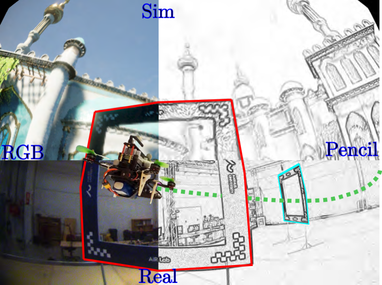
Figure 1: Composed image of simulated (top left) and real (bottom left) gates and converted counterparts (right-hand side) with pencil filter. The perception network is trained solely on simulation data and can accurately perceive racing gates in real-world environments through a fish-eye camera.

Another point to take into consideration is the ease of training the perception network for drone racing. Unlike many robotics applications, the cost to collect labelled high-speed real-world data for drone racing is often prohibitive which limits the use of supervised methods. Therefore, learning through simulation data is understandably much desired [zakharov2019dpod]. For this purpose, [loquercio2018dronet] uses domain randomization for sim-to-real transfer learning with robust performance. A reinforcement learning method is proposed in [song2021autonomous] to learn in simulation a policy for drones that fly at high speeds but reported high tracking errors in practice due to the abstraction from input data to real physical drones is far more complex in reality than in simulation. Unfortunately, none of these methods has been extensively tested under various real-world conditions, such as illumination alterations, which are strongly relevant for drone racing and widely known to negatively affect the performance of perception networks.

In this work, we propose a hybrid DNN-based approach that demonstrates an effective zero-shot sim-to-real transfer learning capability for gate perception in autonomous drone racing navigation. By relying on a smarter input representation using a low-cost morphological operation, called pencil filtering, we can bridge the sim-to-real gap so that our perception network is trained solely in simulation data and works robustly in real-world racing tracks, even under rapid motions and drastic lighting changes. The proposed framework attains a high-speed inference due to the use of our previously proposed efficient backbone network [gatenethuypham2021] with a modification to allow it to work with the new input representation. In our experiments, we show that the performance of the network significantly outperforms the original backbone network [gatenethuypham2021] and other state-of-the-art baseline methods in terms of accuracy and robustness.

The rest of this work is organized as follows. The proposed method for gate perception is detailed in Section II. Section III presents experiments to evaluate the efficiency of the approach against the state-of-the-art baselines. A real-world validation study is presented in Section LABEL:sec:experiment. Finally, Section LABEL:sec:conclusion concludes this work.

II Proposed Method

II-A Pencil Filter

Drastic illumination changes and blurriness caused by rapid flights have been extensively documented in previous work as the main factors behind the performance degradation of visual-based navigation frameworks. In this work, we tackle these challenges by employing an edge-enhancing technique known as the pencil filter [rambach2018learning], but unlike [rambach2018learning], we study its performance under various light intensities and motion blur. The pencil filter applied to an image emphasizes geometrical features, such as edges, corners, and outlines but preserves the overall image structure. This reduces the real-to-sim gap since images from simulation lack accuracy in objects’ sharpness and illumination compared to real images, allowing learning on synthetic data and applying in the real-world environment. In addition, the pencil filter is an illumination agnostic method that keeps the light intensity constant in the images. To extract geometrical features pencil filter first converts an RGB image to a gray-scale format. Then, it applies dilation by convolving the gray-scale image with an ellipse kernel and thresholding to obtain local maxima for each pixel in its neighborhood. This morphological operation generally exaggerates the bright regions of the image. To avoid information loss in the dark regions, the difference in pixel values of the gray-scale image and the dilated one is calculated by normalizing their respective values. The resulting image retains sharp and bolder edges, accentuating object boundaries. Thus, sim-to-real transfer performance is strongly enhanced by converting training RGB images into pencil images. The resulting pencil image is shown on the right-hand side of Fig. 1; while the pseudo-code of the pencil filter is provided in Algorithm 1.

Algorithm 1 Pencil filter.

1:Input: RGB image $\mathbf{I}$

2:Output: pencil image $\mathbf{P}$

3:function pencil_filter($\mathbf{I}$)

4:     $\mathbf{G}\leftarrow\text{grayscale}(\mathbf{I})$

5:     $\mathbf{P}\leftarrow\text{dilate}(\mathbf{G},ellipse)$

6:     for each $y\in[1,\text{rows}(\mathbf{P})]$ do

7:         for each $x\in[1,\text{columns}(\mathbf{P})]$ do

8:              if $\mathbf{P}(y,x)=0$ then

9:                  $\mathbf{P}(y,x)\leftarrow 255$

10:              else

11:                  $\mathbf{P}(y,x)\leftarrow\text{int}\left(255\dfrac{\mathbf{G}(y,x)}{\mathbf{P}(y,x)}\right)$

12:              end if

13:         end for

14:     end for

15:     return $\mathbf{P}$

16:end function

II-B Training Data Generation

The key feature to reduce the gap between simulation and real-world appearance is the use of photo-realistic images. Graphical gaming engines allow simulating intricate ambient effects, mimicking the visual appearance of real environments and the surrounding noise and perturbations. In this work, photo-realistic images are generated by Unreal Engine containing racing scenes with vertical gates in multiple environments with different conditions. Similar to previous drone racing studies in [foehn2020alphapilot, gatenethuypham2021], we use square-shaped gates with checkerboard-like patterns around each corner. To generate a large number of distinct images, a wide-angle RGB camera and the gates are spawned randomly in the environment. They have to be distorted and interpolated to obtain simulated images with the same camera parameters as those from a real camera with a fish-eye lens. Finally, the pencil filter is applied to the fish-eye images. The pipeline for generating training images is depicted in Fig. 2.

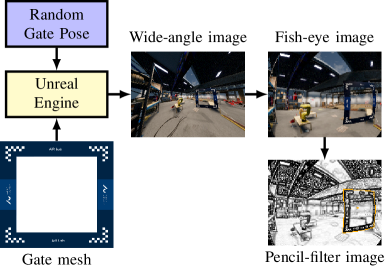
Figure 2: Synthetic images generation pipeline: first, gates are randomly spawned in the simulation environment; then, wide-angle images are distorted with a fish-eye model; finally, the pencil filter is applied.

Using ground-truth information from the simulator, the RGB fish-eye images are labeled with five variables as a tuple $\left\{x,y,d,\theta,c\right\}$. $x$ and $y$ are normalized pixel differences between the top-left corner of the grid and the gate’s center, $d$ is the relative distance to the gate (in meters), and $\theta$ is the relative orientation of the gate (in radians), calculated as the difference between gate’s yaw (heading) and camera’s yaw projected onto the horizontal plane. $c$ is the confidence value of a corresponding grid, which has a value of $1$, if a gate center locates inside, and $0$, otherwise. The training dataset includes more than $30$K samples drawn from 13 different environments with 18 distinct backgrounds and various lighting conditions. Each data sample consists of annotations of the gates and a $160\times 120$ RGB image (illustrated in Fig. 3a). We do not apply any augmentation to the gates and images. In the training phase, the RGB images are converted into corresponding pencil-filtered images (illustrated in Fig. 3b), which retain the same annotations. The advantage of using simulation for data collection is that the data distributions are fully controlled, as shown in Fig. 4a. Note that the training data only contain labels for the front side of a gate, as the back side does not provide relevant information.

(a) Synthetic images after applying fish-eye distortion.

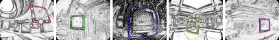
(b) Synthetic images after applying pencil filter.

Figure 3: Samples of the simulation data before (3a) and after (3b) the pencil filter are applied. The images are generated from different domains with varying angles and illumination settings. Note that the training images do not contain bounding boxes of gates, which are illustrated here merely for better visualization.

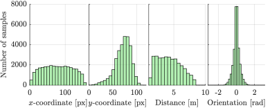
(a) Synthetic training dataset.

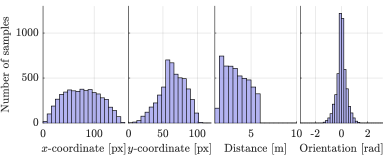
(b) Synthetic testing dataset.

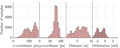
(c) Real-world testing dataset.

Figure 4: Distributions of $x$ and $y$-coordinates, distance and orientation of the gate on images in training and testing datasets.

II-C Backbone Detection Network

The detection network takes a $160\times 120$ image converted by the pencil filter as input before normalization. For feature detection, PencilNet, illustrated in Fig. 5, utilizes as the backbone a convolutional neural network (CNN), from our previous work [gatenethuypham2021], comprising of six 2D convolutional (conv2D) layers with a small number of filters in each layer and one fully-connected (dense) layer to regress detection outputs. The tensors of PencilNet are modified to process one-channel images leading to a smaller number of parameters. Each conv2D layer is followed by a batch normalization and a rectified linear unit (ReLU) activation. Besides, the first five layers use max-pooling with $2\times 2$ kernels. In the last conv2D layer, a small $3\times 5\times 16$ tensor is flattened so that each hidden neuron in the following dense layer can be connected with the extracted features. As in [gatenethuypham2021], the network output is reshaped to $R\times C\times F$, where each grid cell from $R=4$ rows and $C=3$ columns contains regressed $F=5$ values of $\{x,y,d,\theta,c\}$.

Figure 5: Architecture of the proposed method: PencilNet. The pencil filter is applied to RGB images before feeding them to the first conv2D layers. The backbone network is similar to [gatenethuypham2021], with the modification in reducing the number of channels for each filter to work with one-channel input. Each of the first five conv2D layers is followed by a max-pooling with a $2\times 2$ kernel. The tensor in the last conv2D layer is flattened to increase connectivity with the following dense layer. The output tensor is reshaped as a grid of $4\times 3$ cells, where each cell contains five prediction values for pixel offsets to the gate’s center, relative distance and orientation of the gate, and a confidence value.

II-D Training

Similarly to [gatenethuypham2021], PencilNet uses four losses $\mathcal{L}_{xy}$, $\mathcal{L}_{d}$, $\mathcal{L}_{\theta}$ and $\mathcal{L}_{c}$, which are center coordinate, distance, orientation and confidence deviations from true values, respectively:

$$\centering\begin{cases}\mathcal{L}_{xy}&={{\sum_{i=1}^{R}\sum_{j=1}^{C}{\mathds{1}}_{ij}^{\text{obj}}\left[\left(x_{ij}-\hat{x}_{ij}\right)^{2}+\left(y_{ij}-\hat{y}_{ij}\right)^{2}\right],}}\\ \mathcal{L}_{d}&={{\sum_{i=1}^{R}\sum_{j=1}^{C}{\mathds{1}}_{ij}^{\text{obj}}\left(d_{ij}-\hat{d}_{ij}\right)^{2},}}\\ \mathcal{L}_{\theta}&={{\sum_{i=1}^{R}\sum_{j=1}^{C}{\mathds{1}}_{ij}^{\text{obj}}\left(\theta_{ij}-\hat{\theta}_{ij}\right)^{2},}}\\ \mathcal{L}_{c}&={{\sum_{i=1}^{R}\sum_{j=1}^{C}\left[{\mathds{1}}_{ij}^{\text{obj}}+\alpha(1-{\mathds{1}}_{ij}^{\text{obj}})\right]\left(c_{ij}-\hat{c}_{ij}\right)^{2}.}}\\ \end{cases}\@add@centering$$ (1)

The losses are calculated for each grid cell of the output layer with row and column indices $i\in[1,R]$ and $j\in[1,C]$. Terms with the hat operator $(\hat{\star})$ denote predicted values. The term ${\mathds{1}}_{ij}^{\text{obj}}$ is a binary variable to penalize the network only when a gate center locates in a particular grid. The confidence values for grid cells where a gate center does not present is minimized with a weight $\alpha$ so that in run time we can threshold the low confidence predictions, thus reducing false positives. Finally, the loss function is a weighted term:

$$\centering\mathcal{L}=\lambda_{xy}\mathcal{L}_{xy}+\lambda_{d}\mathcal{L}_{d}+\lambda_{\theta}\mathcal{L}_{\theta}+\lambda_{c}\mathcal{L}_{c},\@add@centering$$ (2)

where $\lambda_{xy}$, $\lambda_{d}$, $\lambda_{\theta}$, $\lambda_{c}$ are weights reflecting importance for each of the losses.

III Gate Detection Evaluation

III-A Baseline Methods

In the first part of our study, we evaluate PencilNet performance for the task of racing gate perception with a few notable milestone methods that include DroNet variants (used in [kaufmann2019beauty] and [loquercio2019deep]), and ADRNet variants [jung2018perception]. We also include the performance of our previously published GateNet [gatenethuypham2021], to evaluate the contribution of the pencil filter.

Remark 1

The above baselines are chosen because of their similarities to our method. Some other state-of-the-art baselines such as [foehn2020alphapilot] and [de2021artificial] are not included in this study due to the differences in training data and target outputs.

III-A1 DroNet variants [kaufmann2019beauty, loquercio2018dronet]

A variant of ResNet-8 DNN with three residual blocks is proposed in [loquercio2018dronet] to originally learn a steering policy for a quadrotor to avoid obstacles. However, due to its efficient structure, many subsequent papers utilize it as a backbone feature extractor with different output layers. Kaufmann et al. [kaufmann2019beauty] replace the DroNet’s original output layers with multi-layer perceptron to estimate the mean and variance of the next gate’s pose expressed in spherical coordinates and use the predicted pose for a model predictive control framework to compute a trajectory for the drone. Loquercio et al. [loquercio2018dronet] train DroNet with simulation data using domain randomization and also change the output layers to produce a velocity vector that drives the robot through the gate. Pfeiffer et al. [pfeiffer2022visual] combine DroNet with an attention map as an end-to-end network to capture visual-spatial information allowing the system to track high-speed trajectories. In this work, we compare PencilNet with two variants of DroNet: DroNet-1.0 with the full set of parameters as in [kaufmann2019beauty], and DroNet-0.5 with only half of the filters as in [loquercio2018dronet]. The original output layers are also modified to produce similar outputs as our method for compatibility reasons.

III-A2 ADRNet variant [jung2018perception]

A single-shot object detector based on AlexNet [krizhevsky2012imagenet] is proposed in [jung2018perception] to detect the bounding box of a gate in an image frame, which is used to calculate offset velocities needed to guide a drone past the gate. Since the original ADRNet only detects the gate center and lacks distance and orientation estimation, this work also replaces its output layer with our output layer to predict additional attributes (named ADRNet-mod).

III-A3 GateNet variants [gatenethuypham2021]

To comprehensively evaluate the effect of the pencil filter, PencilNet is compared against the same backbone network, i.e., GateNet, tailored with other edge detection filters. Three different classical filters are considered, namely the Sobel filter [Sobel] and Canny filter [Canny]. Similar to the pencil filter, these filters transform the input images before feeding them to the backbone detection network, as illustrated in Fig. 6.

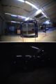
(a)

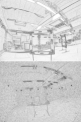
(b)

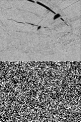
(c)

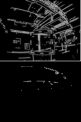
(d)

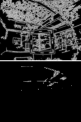
(e)

Figure 6: Visualization of different filters that are considered and evaluated under bright (the first row) and dark (the second row) lighting: (6a) original RGB images, and images converted by (6b) pencil filter, (6c) Sobel filter, (6d) Canny filter, and (6e) Canny filter with a more conservative threshold.

III-B Baselines Training

As mentioned in Section II-B, PencilNet and the other baseline methods are trained with the same simulation dataset containing $160\times 120$ RGB images. Note that filter models, such as the proposed method, apply the respective filter on these images before feeding them into its network. All methods use the same training settings, that is set with a batch size of 32, the initial learning rate of $0.01$, and linearly decayed by $0.1$ at epochs 5 and 8. The models are optimized by Adam [kingma2014adam] with default parameters of $\beta_{1}=0.9$, $\beta_{2}=0.999$, and $\epsilon=10^{-8}$.

III-C Evaluation Metrics

In the evaluation experiments, mean absolute errors (MAE) are calculated for the aforementioned methods as a measure of accuracy in predicting gate’s center on the image plane ($E_{c}$), distance to the gate ($E_{d}$), and orientation of the gate ($E_{\theta}$) relative to the drone’s body frame with the ground-truth information as follows:

$$\centering\begin{cases}E_{c}={\frac{1}{N}\sum_{i=1}^{R}\sum_{j=1}^{C}\left(|\hat{x}_{ij}-x_{ij}|+|\hat{y}_{ij}-y_{ij}|\right)},\\ E_{d}={\frac{1}{N}\sum_{i=1}^{R}\sum_{j=1}^{C}|\hat{d}_{ij}-d_{ij}|},\\ E_{\theta}={\frac{1}{N}\sum_{i=1}^{R}\sum_{j=1}^{C}|\hat{\theta}_{ij}-\theta_{ij}|},\end{cases}\@add@centering$$ (3)

where $N$ is the number of test samples. The metrics in (3) provide the detection accuracy but do not take into account cases where the model fails to make a prediction and, consequently, produces no errors. Therefore, in addition to the metrics in (3), we consider another metric that calculates the percentage of false negative (FN) predictions, i.e., the number of times a network does not detect a gate present in the image over the total number of samples. If a method produces a high FN, it performs poorly even though the other metrics may appear decent.

III-D Sim-to-Sim and Sim-to-Real Evaluation