Signature of parity anomaly in the measurement of optical Hall conductivity in quantum anomalous Hall systems

Abstract

Parity anomaly is a quantum mechanical effect that the parity symmetry in a two-dimensional classical action is failed to be restored in any regularization of the full quantum theory and is characterized by a half-quantized Hall conductivity. Here we propose a scheme to explore the experimental signature from parity anomaly in the measurement of optical Hall conductivity, in which the optical Hall conductivity is nearly half-quantized for a proper range of frequency. The behaviors of optical Hall conductivity are studied for several models, which reveal the appearance of half-quantized Hall conductivity in low or high frequency regimes. The optical Hall conductivity can be extracted from the measurement of Kerr and Faraday rotations and the absorption rate of the circularly polarized light. This proposal provides a practical method to explore the signature of parity anomaly in topological quantum materials.

I Introduction

Parity anomaly describes the fact that a single massless Dirac fermion in 2+1 dimensions undergoes a spontaneous symmetry breaking when it is coupled to the $U(1)$ gauge field [2, 1, 3]. This anomalous effect is physically manifested as the half-quantized Hall conductivity in the external electromagnetic field. Several condensed matter systems have been proposed to simulate parity anomaly on a lattice, such as a monolayer graphite [4, 5] and PbTe-type narrow-gap semiconductor with an anti-phase boundary [6]. In addition, the massive Dirac fermions break the time-reversal symmetry and parity symmetry explicitly. At the half-filling, the finite Dirac mass also leads to a half-quantized Hall conductivity [5, 8, 7, 9]. Combined with the parity anomaly, the massive Dirac fermion exhibits an integer-quantized Hall conductivity, which leads to the quantum anomalous Hall effect in condensed matter systems [11, 12, 10, 13, 14].

As the contribution from the parity anomaly and Dirac mass are mixed together, it is difficult to distinguish the two mechanisms from the total Hall conductivity in the dc limit. In 1988, Haldane proposed that the half-quantized Hall conductivity from the parity anomaly could be realized if an unpaired Dirac fermion appears at a critical transition point between a normal insulator and a Chern insulator phase [5]. In recent, another attempt was reported in the semi-magnetic topological insulator thin film, where only the top surface state was gapped by the magnetic doping, and a nearly half-quantized Hall conductivity was observed [15]. Nevertheless, it is known that a single symmetry-protected Dirac fermion does not exist on a two-dimensional lattice [16]. Hence, it is desired to explore a new method to figure out the half-quantized Hall conductivity from the parity anomaly from a system where a single gapless Dirac point cannot be realized. Fortunately, the physical origins of two half-quantized Hall conductivities of the massive Dirac cone are different, one is attributed by the low energy fermions around the Dirac cone and the high energy regulator part respectively. Thus they can be distinguished at different energy scales by optical Hall conductivity.

Recently, Tse and MacDonald proposed that Hall conductivity at finite frequencies can be detected using the magneto-optical technique. This is mainly reflected in that the Kerr and Faraday angles can be experimentally implemented to detect the optical Hall conductivity of the system[18]. However, this series of work has mainly focused on the low energy region of the Dirac cone, and the contribution of quantum anomalies from the high energy region has yet to be explored[18, 20, 17, 21, 22, 23, 24, 25, 19]. Meanwhile, the magneto-optical effect is naturally suited for exploring response patterns in the high-energy region, which provides us a possible way to detect the signature of parity anomalies.

In this paper, we propose a method to detect the signature of parity anomaly in a condensed matter system and to distinguish different origins of the anomalous quantum Hall effect. We first calculate the optical Hall conductivity of the Wilson fermions and massive Dirac fermions analytically and get the expression of half-quantized Hall conductivity by making Taylors expansion at the proper frequency. Besides, we calculate the Hall conductivity of different lattice models, including the Bernevig-Hughes-Zhang (BHZ) model, the Haldane model, and the magnetically doped topological insulator thin films. Finally, we discuss how this phenomenon can be implemented experimentally and the effect that temperature and disorder can have on this, and we propose that the character of this optical Hall conductivity can be measured by several magneto-optical effects.

II Model Hamiltonian

We begin with the two-dimensional Wilson fermion model [27, 26]

$$H=v\hbar(k_{x}\sigma_{x}+k_{y}\sigma_{y})+(mv^{2}-b\hbar^{2}k^{2})\sigma_{z},$$ (1)

where $v$ is the effective velocity, $k_{i}$ with $i=x,y$ are wave vectors, $k^{2}=k_{x}^{2}+k_{y}^{2}$, and $\sigma_{i}$ with $i=x,y,z$ are the Pauli matrices. $2mv^{2}$ is the band gap at $k=0$, $b\hbar^{2}k^{2}$ is the dynamical mass regulator. In the dc limit, when the chemical potential is located with the band gap, i.e., at half filling, the Hall conductivity of the system is

$$\sigma_{xy}=\frac{1}{2}\frac{e^{2}}{h}[{\rm sgn}(m)+{\rm sgn(b)}]$$ (2)

[29, 30, 28]. Either the band gap $mv^{2}$ and the regulator $b\hbar^{2}k^{2}$ contribute $\frac{1}{2}\frac{e^{2}}{h}$ to the Hall conductivity, which only depends on the signs, not value of the two mass terms. When $m$ and $b$ have the same sign, i.e., $bm>0$, the Hall conductivity is quantized to be one in the unit of $e^{2}/h$, and the system is is topologically non-trivial. When $m$ and $b$ have the opposite signs, i.e., $bm<0$, the Hall conductivity is equal to zero, and the system is is topologically non-trivial. In the absence of the regulating term $b\hbar^{2}k^{2}$, the Hall conductivity is $\sigma_{xy}=\frac{1}{2}\frac{e^{2}}{h}{\rm sgn}(m)$, which contradicts the Thouless-Kohmoto-Nightingale-Nijs (TKNN) quantization rule in a gapped system [31]. This means it cannot exist on a two-dimensional lattice. The presence of the regulator $b\hbar^{2}k^{2}$ which provides another half-quantized Hall conductivity as $\frac{1}{2}\frac{e^{2}}{h}{\rm sgn}(b)$, is essential to avoid the contradiction. When $m=0$, and the band gap closes, the half-quantized Hall conductivity from the regulator $b\hbar^{2}k^{2}$ can exist alone [32, 33]. In the case the parity is broken by the presence of he regulator $b\hbar^{2}k^{2}$. However, when $b\rightarrow 0$, the parity symmetry is restored, and the Hall conductivity is still equal to $\frac{1}{2}\frac{e^{2}}{h}{\rm sgn}(b)$, not zero as expected in the parity symmetry. This is the so-called the parity anomaly in the lattice gauge theory [26].

In the dc case, the Hall conductivity is equal to one or zero. We cannot distinguish the contribution from the he band gap $mv^{2}$ and the regulator $b\hbar^{2}k^{2}$. As the two terms dominate the low energy region ($k\rightarrow 0$) and high energy regime ($k\rightarrow+\infty$) separately, the two parts will respond disparately to an incident electromagnetic field with a finite-frequency. Thus the optical Hall conductivity may provide a possible way to distinguish the contribution at different energetic scales.

III Optical Hall conductivity

In this section, we will present the optical Hall conductivity at a finite-frequency. In general, the optical Hall conductivity $\sigma_{xy}(\omega)$ at finite-frequency $\omega$ can be evaluated from the Kubo formula

$$\sigma_{xy}(\omega) =ie^{2}\hbar\int\frac{d^{2}k}{(2\pi)^{2}}\sum_{m,n}\frac{v_{mn}^{x}v_{nm}^{y}}{\epsilon_{m}-\epsilon_{n}-\hbar\omega+i\delta}\frac{f(\epsilon_{m})-f(\epsilon_{n})}{\epsilon_{n}-\epsilon_{m}},$$ (3)

where $\epsilon_{n}$ is the energy eigenvalue of state $|n\rangle$ , $v_{mn}^{a}(k)=\frac{1}{\hbar}\langle m|\frac{\partial H}{\partial k_{a}}|n\rangle$ are the matrix elements of the velocity operators at $a=x,y$ direction, and $f(\epsilon)=1/\left(1+\exp(\frac{\epsilon-\mu}{k_{B}T})\right)$ is the Fermi-Dirac distribution function with $\mu$ the chemical potential at finite temperature $T$. $k_{B}$ is the Boltzmann constant. $\delta$ is the infinitesimal regulator. After some calculations, the real part of the optical Hall conductivity at zero temperature ($k_{B}T=0$) and $\mu=0$ can be analytically found as (see Appendix for details)

$$\mathrm{Re}\sigma_{xy}(\omega)=\frac{e^{2}}{h}\frac{1}{8\xi\tilde{\omega}}\left[2(1-4bm)\ln\left|\frac{\tilde{\omega}+\xi}{\tilde{\omega}-\xi}\right|+\sum_{s=\pm}g_{s}(\omega)\right],$$ (4)

where the dimensionless parameter $\xi=\sqrt{1-4bm+\tilde{\omega}^{2}}$ and the renormalized frequency $\tilde{\omega}=b\hbar\omega/v^{2}$, and

$$g_{s}(\omega)=(1-4bm-s\xi)\ln\left|\frac{\xi(1-2bm)-2b|m|\tilde{\omega}-s(1-4bm)}{\xi(1-2bm)+2b|m|\tilde{\omega}-s(1-4bm)}\right|.$$

In the dc limit by taking $\omega\to 0$, it recovers the Hall conductivity $\sigma_{xy}(0)=\frac{1}{2}\frac{e^{2}}{h}[{\rm sgn}(m)+{\rm sgn}(b)]$ as shown in Fig. 1. In the case of $m>0$ and $b>0$, $\sigma_{xy}(0)=\pm\frac{e^{2}}{h}$ and in the case $m<0$ and $b>0$, $\sigma_{xy}(0)=0$. The blue and yellow lines represent the two cases separately.With the frequency increasing, the Hall conductivity deviates from the dc limit value and becomes divergent at $\hbar\omega=mv^{2}$ due to the Rabi resonance. This a strong indication of the existence of the band gap $mv^{2}\neq 0$. Near the region, the sign of the Hall conductivity depends on the sign of $m$ . As the frequency further increases above the band gap $\hbar\omega>mv^{2}$, the Hall conductivities converge to a quasi-quantized plateau with a half-integer value $\frac{1}{2}\mathrm{sgn}(b)\frac{e^{2}}{h}$. When the frequency is in the proper range , $mv^{2}\ll\hbar\omega\ll\frac{v^{2}}{b}$, i.e., the dimensionless parameters $\tilde{\omega},\frac{bm}{\tilde{\omega}}\ll 1$, the real part of $\sigma_{xy}(\omega)$ is approximately,

$$\mathrm{Re}\sigma_{xy}(\omega)\approx\frac{e^{2}}{2h}\mathrm{sgn}(b)\left[1+\mathrm{sgn}(bm)\left(\frac{2bm}{\tilde{\omega}}\right)^{2}\right].$$ (5)

The value of the plateau is independent of the magnitude and sign of $m$, but is attributed by the sign of $b$, which can be regarded as a signature of parity anomaly. $\mathrm{Re}\sigma_{xy}(\omega)$ will deviate the value of plateau if the frequency continues increasing,

$$\mathrm{Re}\sigma_{xy}(\omega)\approx\frac{e^{2}}{2h}\mathrm{sgn}(b)\left[1-\frac{2}{3}\tilde{\omega}^{2}\right].$$ (6)

For comparison, we also plot $\mathrm{Re}\sigma_{xy}(\omega)$ for the massive Dirac fermions ($m>0$ and $b=0$). The value decreases to zero quickly after the Rabi resonance, and there is no signature of parity anomaly.

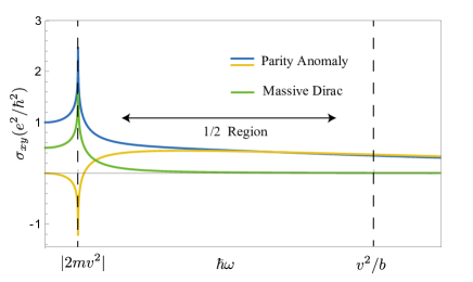
Figure 1: The comparison of optical Hall conductivity between massive Dirac fermions and Wilson fermions. The blue and yellow lines are Wilson fermions that are topologically non-trivial and trivial, respectively. The green line is the massive Dirac fermion. The region sandwiched between two dashed lines is the half-quantization region from the parity anomaly. Here $mv^{2}=0.05\,{\rm eV}$ (green and blue line), $-0.05\,{\rm eV}$ (yellow line), $v\hbar=0.5\,{\rm eV}\cdot\textrm{\r{A}},$ and $b\hbar^{2}=0.2\,{\rm eV}\cdot\textrm{\r{A}}^{2}$

Besides the dynamical mass, the massive Dirac fermion with mass $m$ can also be regulated by another Dirac fermion with a large Dirac mass $M$, which is the Pauli-Villars method [34]. In the case, the real part of the optical Hall conductivity can be found to be

$$\mathrm{Re}\sigma_{xy}(\omega) =\frac{1}{2}\frac{e^{2}}{h}\Big{(}\frac{mv^{2}}{\hbar\omega}\ln\left|\frac{\hbar\omega+2|m|v^{2}}{\hbar\omega-2|m|v^{2}}\right|$$

$$+\frac{Mv^{2}}{\hbar\omega}\ln\left|\frac{\hbar\omega+2|M|v^{2}}{\hbar\omega-2|M|v^{2}}\right|\Big{)}.$$ (7)

In the dc limit of $\omega\to 0$, it is reduced to

$$\mathrm{Re}\sigma_{xy}(\omega\to 0)=\frac{1}{2}\frac{e^{2}}{h}[{\rm sgn}(m)+{\rm sgn}(M)].$$ (8)

Similar to the case of Wilson fermion, the zeroth-order of Hall conductivity is half-quantized and merely depends on the sign of the regulator $M$. Therefore, the effect of the large mass regulator $M$ contributes a background of half-quantized Hall conductivity and shifts the whole curve by $\frac{1}{2}\frac{e^{2}}{h}\mathrm{sgn}(M)$.

The optical Hall conductivity will be divergent when the frequency $\omega$ approaches the band edges $2mv^{2}$ and $2Mv^{2}$. When $2mv^{2}\ll\hbar\omega\ll 2Mv^{2}$, the real part of the optical Hall conductivity can be expressed appropriately as following,

$$\sigma_{xy}\approx\frac{\mathrm{sgn}(M)}{2}\frac{e^{2}}{h}\left[1+\frac{1}{12}\left(\frac{\hbar\omega}{Mv^{2}}\right)^{2}+4{\rm sgn}(mM)\left(\frac{mv^{2}}{\hbar\omega}\right)^{2}\right].$$ (9)

Thus in the presence of Pauli-Villars regulator, the finite-Hall conductivity shows similar signature of parity anomaly as a half-quantized plateau.

IV Lattice Realization

The formulation of the lattice theory of Dirac fermion is closely related to the Nielsen-Ninomiya no-go theorem [7]. Unlike the continuum model, the finite lattice spacing serves as a natural UV regulator. The Wilson fermion in Eq. (1) can be directly put on the lattice with no fermion doubling problem in the presence of the regulation term $b(\hbar k)^{2}\sigma_{z}$, which is equivalent to spin-polarized Bernevig-Hughes-Zhang (BHZ) model [35],

$$H_{BHZ}(k_{x},k_{y}) =v\frac{\hbar}{a}\sum_{i=x,y}\sin(k_{i}a)\sigma_{i}$$

$$+mv^{2}\left\{1-2bm\left(\frac{\hbar}{mva}\right)^{2}[2-\sum_{i=x,y}\cos(k_{i}a)]\right\}\sigma_{z},$$ (10)

where $a$ is the lattice constant. The Chern number of the valence band of this model depends on the the Dirac mass $m$ and the coefficient $b$,

$$C =\frac{1}{2}\mathrm{sgn}(m)\Big{\{}2\mathrm{sgn}\left[1-4bm\left(\frac{\hbar}{mva}\right)^{2}\right]$$

$$-\mathrm{sgn}\left[1-8bm\left(\frac{\hbar}{mva}\right)^{2}\right]-1\Big{\}}.$$ (11)

By numerically evaluating the Kubo formula in Eq. (3), we obtain the optical Hall conductivity in Fig. 2 for three different band gaps ($mv^{2}=-0.1,0.05,0.1\,\mathrm{eV}$) in Eq. (10) . When $mv^{2}=0.05\mathrm{eV}$ and $mv^{2}=0.1\mathrm{eV}$, the Chern number is $C=1$, and the optical Hall conductivities begin with $\frac{e^{2}}{h}$ at $\omega=0$ and becomes divergent at $\hbar\omega=0.1\,\mathrm{eV}$ and $\hbar\omega=0.2\,\mathrm{eV}$, respectively. When $mv^{2}=-0.1\,{\rm eV},$ $C=0$, and the optical Hall conductivity begins with $0$ at $\omega=0$ and become divergent at $\hbar\omega=0.2\,\mathrm{eV}$. In a large frequency regime $mv^{2}\ll\hbar\omega\ll\frac{v^{2}a^{2}}{b}$, all the three curves approach $\frac{1}{2}\frac{e^{2}}{h}$ (as indicated by the black line), which is consistent with the results of continuum model in Fig. 1. In experiments, the spin-polarized BHZ models can be realized in several two-dimensional quantum anomalous Hall effect materials, including monolayer magnetic material $1T-\mathrm{VSe}_{2}$ [36], and 2D magnetic Van der Waals heterojunction of $\mathrm{MnNF}/\mathrm{MnNCl}$ [37].

large

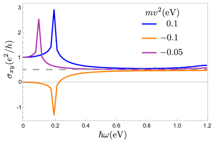
Figure 2: The Hall conductivity with finite-frequency of BHZ model with different gaps. The different colors represent the different mass gap of the model and the sign indicates the topologically trivial or non-trivial. All samples have a plateau tending to 1/2 at the proper frequency. The different line represent different mass show in the legends with $v\hbar=0.5\,{\rm eV}\cdot\textrm{\r{A}},b\hbar^{2}=0.2\,{\rm eV}\cdot\textrm{\r{A}}^{2},a=1{\rm nm}.$

The first lattice model to realize parity anomaly was proposed in the seminal paper by Haldane [5]. The Haldane model can be implemented in a honeycomb lattice with the nearest hopping $t$ and the next to nearest imaginary hopping $t^{\prime}$ and an on-site potential $M$. In terms of the Pauli matrices, the corresponding tight-binding model can be expressed as

$$H=\sum_{i=x,y,z}d_{i}\sigma_{i},$$ (12)

where $d_{x}(\mathbf{k})=t\sum_{i}\cos(\mathbf{k}\cdot\mathbf{a}_{i})$, $d_{y}(\mathbf{k})=t\sum_{i}\sin(\mathbf{k}\cdot\mathbf{a}_{i})$, $d_{z}(\mathbf{k})=\Delta-2t^{\prime}\sum\sin(\mathbf{k}\cdot\mathbf{b}_{i})$, $\mathbf{a}_{i}$ is the nearest vectors of honeycomb lattice that $\mathbf{a}_{1}=(\frac{1}{2},\frac{\sqrt{3}}{2})a$, $\mathbf{a}_{2}=(\frac{1}{2},-\frac{\sqrt{3}}{2})$a, $\mathbf{a}_{2}=(-1,0)a$, and $\mathbf{b}_{i}=\epsilon_{ijk}(\mathbf{a}_{j}-\mathbf{a}_{k})$ with $\epsilon_{ijk}$ the anti-symmetric symbol. There are two Dirac cones at $K$ and $K^{\prime}$ valleys in the corner of the Brillouin zone, with the band gaps $2\Delta_{+}=2\Delta+6\sqrt{3}t^{\prime}$ and $2\Delta_{-}=2\Delta-6\sqrt{3}t^{\prime}$ respectively. When one of the band gaps closes (e.g., $\Delta=3\sqrt{3}t^{\prime}$), the low energy theory is described by a single massless Dirac fermion with the parity symmetry (or time-reversal symmetry). The massive Dirac fermion at the other valley plays the role of the large mass regulator and gives a half-quantized contribution to the Hall conductivity, $\sigma_{xy}=\frac{1}{2}\frac{e^{2}}{h}.$ Haldane thought that it is a realization of parity anomaly on the lattice. As shown in Fig. 3(a), there are two peaks in the optical Hall conductivity when $\hbar\omega=2\Delta_{+}$ or $\hbar\omega=2\Delta_{-}$, and the conductivity drops to zero quickly when $\hbar\omega$ is larger than $2\Delta_{+}$. However, when $2\Delta_{-}<\hbar\omega\ll 2\Delta_{+}$, the optical Hall conductivity is approximately half-quantized. This condition can be realized by tuning the band gap of two valleys in a Floquet system [38, 39]. Hence, the optical Hall conductivity can be used to distinguish the contribution from the low energy physics and the high energy physics (or the parity anomaly). The Haldane model can be realized in ferromagnetic honeycomb materials with no inversion symmetry [40, 41]. Recently, some Moiré materials are reported that spontaneous magnetization at a proper filling have a similar valley polarized quantum Hall behavior [44, 43, 42]. As the half-quantization of the optical Hall conductivity does not require $\Delta_{-}=0$ exactly, it becomes more feasible in experiments.

In addition to the Haldane model, the magnetically doped topological insulator thin film, which is the first realization of the quantum anomalous Hall system experimentally[11, 12], also yields two Dirac cones. Different from the Haldane model, the two Dirac cones in topological insulators are separated in the real space and located on the top and bottom surfaces, respectively. The magnetic doping will open band gaps for the surface Dirac cones through the exchange interaction [45, 46]. Then, each of the two Dirac cones contributes a one-half Hall conductivity individually [33]. In the quantum anomalous Hall insulator phase, the summation of two surfaces Dirac cones gives a quantized Hall conductivity. Here we use the magnetically doped three dimensional topological insulator model to perform the calculation,

$$H_{3D} =ig(z)\alpha_{1}\alpha_{2}+v\frac{\hbar}{a}\sum_{i=x,y,z}\sin(k_{i}a)\alpha_{i}$$

$$+m_{0}v^{2}\left\{1-b_{0}\left(\frac{\hbar}{m_{0}va}\right)^{2}[3-\sum_{i=x,y,z}\cos(k_{i}a)]\right\}\beta,$$ (13)

where $\alpha_{i}=\tau_{1}\sigma_{i}$ and $\beta=\tau_{3}\sigma_{0}$ are the Dirac matrices, and $a$ is the lattice constant. $v,b_{0}$ and $m_{0}$ are material parameters for a three-dimensional topological insulator. The term $ig(z)\alpha_{1}\alpha_{2}$ is the position-dependent Zeeman energy along the $z$-direction, which breaks the time-reversal symmetry and generates the Dirac mass in the surface states. When $g(z)\equiv g$ is chosen as a constant, the induced Dirac masses of top and bottom surface states will have the same magnitude and opposite sign. Besides, the two surface states have opposite helicity [30]. Then, in the dc limit, each of them contributes $\frac{e^{2}}{2h}\mathrm{sgn}(g)$ to the Hall conductivity, and the total Hall conductivity is quantized as $e^{2}/h$. When the frequency is nonzero, the system hosts the inversion symmetry and the optical Hall conductivity from the two massive surface states is still identical, as shown in Fig. 3(b). The total optical Hall conductivity of the magnetic topological insulator thin film can be regarded as twice of the massive Dirac fermion without any regulator. It confirms the fact that the quantized Hall conductivity in the magnetically doped topological insulators is determined by two gapped surface states. This mechanism would make the behavior of optical Hall conductivity in magnetic topological insulators different from the case of the Haldane model. The optical Hall conductivity can be used to distinguish multiple physical origins of quantum anomalous Hall effect in different systems.

Moreover, if $g(z)$ is mainly localized at the top surface, it is possible to open the gap of the top surface state only while the bottom surface state remains gapless. It provides the most direct way to realize the parity anomaly in experiments [15, 33]. However, it is challenge to preserve a single gapless surface state. In such a case, parity anomaly can also be detected by the optical Hall conductivity. When there is a significant difference in the magnitude of the band gaps for the two Dirac states, it will be similar to the Haldane model. A half-quantized plateau can also occur if the frequency is between the band gaps of the two Dirac cones.

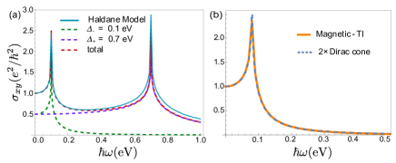
Figure 3: (a). The solid line is the optical Hall conductivity for the Haldane model, and the dashed lines are the optical Hall conductivity for the massive Dirac model, where the gaps equal $\Delta_{-}=0.1\,\mathrm{eV}$ and $\Delta_{+}=0.7\,\mathrm{eV}$ and hopping strength is chosen as $t=0.5\,{\rm eV}$. (b). The optical Hall conductivity for the magnetically doped topological insulator thin film of 8 quintuple layer with the Zeeman term $g=0.04\,\mathrm{eV}$. The orange solid line is the numerical result of optical Hall conductivity and the dashed line is twice of the analytical result of a massive Dirac fermion. The parameters for the topological insulator are chosen as $m_{0}v^{2}=0.68\,\mathrm{eV},$ $v\hbar=0.4\,\mathrm{eV}\cdot\textrm{\r{A}},$ and $b_{0}\hbar^{2}=1.4\,\mathrm{eV}\cdot\textrm{\r{A}}^{2},a=1{\rm nm}$.

V Experiment Implement

In experiment, the optical Hall conductivity can be obtained by measuring the magneto-optical effect, which reflects the information of Hall conductivity near the sample surface.

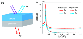
Figure 4: (a).The experiment setup for the measurement of Kerr and Faraday angle. (b). The Kerr and Faraday angle of the the BHZ model (blue and cyan dashed lines) and the magnetic topological insulator film (red and cyan dashed lines).The parameters of the corresponding model are the same as the one below the Fig. 2 and Fig. 3. The refractive index of the substrate is chosen as $n_{r}=3.46$ for InP.

As shown in figure. 4(a), we takes the sample on the substrate with the refractive index $n_{r}>1,$ and inject a light linearly polarized in the $x$ direction with frequency $\omega$, the electric field of the light is ${\bf E}_{in}=E_{0}e^{i(\omega t-kx)}\hat{x}$. In terms of electric field of transmission light ${\bf E}_{t}$ and the reflection light as ${\bf E}_{r}$, the Kerr and Faraday angles are defined by the $\tan\theta_{K}=E_{r}^{y}/E_{r}^{x}$ and $\tan\theta_{F}=E_{t}^{y}/E_{t}^{x}$, respectively. The two angles can be solved by the Maxwell equation with proper boundary condition (see Appendix B) as

$$\tan\theta_{F}= \frac{2\alpha\tilde{\sigma}_{xy}}{1+n_{r}+2\alpha\tilde{\sigma}_{xx}},$$ (14)

$$\tan\theta_{K}= -\frac{4\alpha\tilde{\sigma}_{xy}}{n_{r}^{2}-1+4\alpha[\tilde{\sigma}_{xx}(n_{r}+\alpha\tilde{\sigma}_{xx})+\alpha\tilde{\sigma}_{xy}^{2}]},$$ (15)

where the dimensionless $\tilde{\sigma}_{xx}=\sigma_{xx}\frac{h}{e^{2}}$ and $\tilde{\sigma}_{xy}=\sigma_{xy}\frac{h}{e^{2}}$ are the dimensionless transverse conductivity and the Hall conductivity, respectively, and $\alpha\approx 1/137$ is the fine structure constant. When $\tilde{\sigma}_{xx}$ and $\tilde{\sigma}_{xy}$ are much smaller than $\alpha^{-1}$ and the refractive index of the substrate $n_{r}>1$, the two angles can be approximated as $\theta_{F}=\arctan\frac{2\alpha}{1+n_{r}}\tilde{\sigma}_{xy}$ and $\theta_{K}=-\arctan\frac{4\alpha}{n_{r}^{2}-1}\tilde{\sigma}_{xy}$, respectively. In Fig. 4(b), we plot $\theta_{F}$ and $-\theta_{K}$ as functions of $\omega$ for the magnetic topological insulator and BHZ model. We consider the case that the wavelength of light is much larger than the thickness of the sample i.e., $d\ll\lambda$ and the insulating subtract is InP with $n_{r}=3.46$ [15]. In this limit, the bottom and top surfaces can be viewed as a whole. Therefore, $\sigma_{xx}$ and $\sigma_{xy}$ in Eq. (14) and (15) denote the total longitudinal and Hall conductivities from two surfaces, respectively. At zero frequency, the chemical potential inside Dirac gap of both surfaces, we have $\sigma_{xx}=0$ and $\sigma_{xy}=e^{2}/h$, the Faraday and Kerr angles have universal values $\theta_{F}\approx 3.28\times 10^{-3}\,{\rm rad}$ and $\theta_{K}\approx-2.66\times 10^{-3}\,{\rm rad}$.. At finite frequencies, the $\theta_{F}$ and $\theta_{K}$ for the BHZ model display a plateau with half of the zero frequency value for $\hbar\omega\gg 2|m|v^{2}$. As indicated by the red and cyan dashed lines in Fig. 4(b), the Kerr and Faraday angles of magnetic topological insulator film drop to zero after $\hbar\omega\gg 2g$, which display the same character as the Hall conductivity in Fig. 3(b).

Furthermore, the optical Hall conductivity can be deduced from the absorption rate of the circularly polarized light $\Gamma_{\pm}(\omega)$ [47]. The imaginary part of optical Hall conductivity can be related to the difference between the absorption rate of the left-hand and the right-hand light as $\mathrm{Im}\sigma_{xy}(\omega)=\hbar\omega(\Gamma_{+}-\Gamma_{-})/(8AE^{2}),$ where $E$ is the intensity of light and $A$ is the area of the sample. From the Kramers-Kronig relation, the real part of the optical Hall conductivity can be obtained as $\mathrm{Re}\sigma_{xy}(\omega)=\frac{2}{\pi}{\cal P}\int_{0}^{\infty}\frac{\omega^{\prime}\mathrm{Im}\sigma_{xy}(\omega^{\prime})d\omega^{\prime}}{\omega^{\prime 2}-\omega^{2}}$ with $\mathcal{P}$ denoting the Cauchy principal value, and the half-quantized plateau can be found at finite-frequency in the $\mathrm{Re}\sigma_{xy}.$

VI Discussion and summary

Besides the light frequency, disorder and temperature can also be used to smear off the low energy contribution in the Hall conductivity and leave the parity anomaly contribution from the high energy only [24]. Therefore, we can expect a similar half-quantized plateau in the Hall conductivity at finite temperature or finite disorder. For the disordered system, using the Born approximation, the disorder effect can be introduced phenomenologically by the quasi-particle self-energy $\Gamma$ in the Green function, i.e. $G^{r/a}=(i\omega_{n}-H\pm i\Gamma)^{-1}.$ Thus, the Hall conductivity in the presence of disorder can be expressed as

$$\sigma_{xy}=e^{2}\hbar\int\frac{d^{2}k}{(2\pi)^{2}}\sum\frac{\mathrm{Im}(v_{mn}^{x}v_{nm}^{y})[f(\epsilon_{m})-f(\epsilon_{n})]}{(\epsilon_{m}-\epsilon_{n})^{2}+\Gamma^{2}}.$$ (16)

Compared to the Kubo formula at finite-frequency, $\sigma_{xy}$ can be obtained by taking an Analytic continuation that replace the frequency $\hbar\omega$ with $i\Gamma$. When $mv^{2}\ll\Gamma\ll\frac{v^{2}}{b},$ The asymptotic behavior of Hall conductivity reads

$$\mathrm{Re}\sigma_{xy}(\Gamma)=\frac{e^{2}}{2h}{\rm sgn}(b)\left[1+\frac{2}{3}\left(\frac{b\Gamma}{v^{2}}\right)^{2}-\mathrm{sgn}(mb)\left(\frac{2mv^{2}}{\Gamma}\right)^{2}\right],$$ (17)

where the leading order is a half-quantized value $\frac{1}{2}{\rm sgn}(b)$.

In addition to disorder in the system, the temperature can also lead to the half-quantized plateau when the temperature $k_{B}T$ satisfies that $mv^{2}\ll k_{B}T\ll\frac{v^{2}}{b}.$ The effect of the temperature can be seen as averaging the Berry curvature of the conduction band and valence band near the Fermi surface, which can erase the contribution of the low energy part, and only the contribution from the high energy part remains. This also separates the parity anomaly part and allows the system to show the half-quantized plateau. We plot the Hall conductivity as a function of temperature $k_{B}T$ and the self-energy $\Gamma$ in the same dimensionless energy scale in Fig.5. The Hall conductivity shows a similar nearly half-quantized feature as the optical Hall conductivity in Fig.1.

Figure 5: The Hall conductivity of Wilson fermion as functions of temperature(pink line) and disorder(cyan line), the temperature $k_{B}T$ and the disorder $\Gamma$ have been renormalized into the same dimensionless energy scale. The parameters are $v\hbar=0.5\,\mathrm{eV}\cdot\textrm{\r{A}},b\hbar^{2}=0.2\,\mathrm{eV}\cdot\textrm{\r{A}}^{2},mv^{2}=0.05\,{\rm eV}.$

In quantum anomalous Hall systems, the quantized Hall conductivity usually consists of two parts, one is the contribution from massive Dirac cone and the other is the parity anomaly contribution in the high energy region. In this article, the finite-frequency method is introduced to separate these two different sources of Hall conductivity. When the applied frequency is in the proper interval, the Hall conductivity of the system exhibits a half-quantized plateau, and this plateau is considered a direct manifestation of the parity anomaly. Thus in the condensed matter system, the half-quantized optical Hall conductivity can be used as a marker to characterize the parity anomaly.

Appendix A Calculation of Optical Hall conductivity

For a general $2\times 2$ matrix Hamiltonian in the form $H={\bf d}\cdot\sigma$ with $\mathbf{d}=(d_{x},d_{y},d_{z})$, the eigenenergy and eigenstates can be found as

$$E_{\chi} =\chi\sqrt{d_{x}^{2}+d_{y}^{2}+d_{z}^{2}}=\chi d,$$

$$|\phi_{\chi}\rangle =\begin{pmatrix}\frac{\hat{d}_{x}-i\hat{d}_{y}}{\sqrt{2(1-\chi\hat{d}_{z})}}\\ \frac{1-\hat{d}_{z}}{\sqrt{2(1-\chi\hat{d}_{z})}}\end{pmatrix},$$

where $\chi=+$ is for the conduction band and $\chi=-1$ is for the valence band. $\hat{d_{i}}$ with $i=x,y,z$ are defined as $\hat{d_{i}}=d_{i}/d$.

In the eigen energy basis, the matrix elements of the velocity operators are defined as

$$v_{\chi\chi^{\prime}}^{x} =\frac{1}{\hbar}\sum_{i=x,y,z}\frac{\partial d_{i}}{\partial k_{x}}\langle\phi_{\chi}|\sigma_{i}|\phi_{\chi^{\prime}}\rangle,$$

$$v_{\chi\chi^{\prime}}^{y} =\frac{1}{\hbar}\sum_{i=x,y,z}\frac{\partial d_{i}}{\partial k_{y}}\langle\phi_{\chi}|\sigma_{i}|\phi_{\chi^{\prime}}\rangle.$$

After a straightforward calculation, one can obtain the imaginary part of the velocity product as

$${\rm Im}(v_{\chi\bar{\chi}}^{x}v_{\bar{\chi}\chi}^{y})=\chi\frac{d^{2}}{\hbar^{2}}\hat{\mathbf{d}}\cdot(\partial_{x}\hat{\mathbf{d}}\times\partial_{y}\hat{\mathbf{d}}).$$

For the BHZ model, $\mathbf{d}=(v\hbar k_{x},v\hbar k_{y},mv^{2}-bk^{2}\hbar^{2})$ and $d=\sqrt{v^{2}\hbar^{2}k^{2}+(mv^{2}-bk^{2}\hbar^{2})^{2}}$, we have ${\rm Im}v_{\chi\bar{\chi}}^{x}v_{\bar{\chi}\chi}^{y}=\chi\frac{v^{2}}{d}(mv^{2}+b\hbar^{2}k^{2})$. As a result, the real part of the optical Hall conductivity at zero temperature in Eq. (3) is given by

$${\rm Re}\sigma_{xy}(\omega)=\frac{e^{2}}{h}\frac{1}{8\xi\tilde{\omega}}\sum_{s}\left(1-4bm+s\xi\right)$$

$$\times\mathrm{arcoth}\left.\left(\frac{2\frac{b\hbar k}{v}\tilde{\omega}\sqrt{1+(\frac{mv}{\hbar k}-\frac{b\hbar k}{v})^{2}}}{s(1-4bm)+\xi\left(1-2bm+2\left(\frac{b\hbar k}{v}\right)^{2}\right)}\right)\right|_{0}^{+\infty}.$$ (18)

Here $\xi$ and $\tilde{\omega}$ is as the same definition as in the main text. Using the analytical continuation $\mathrm{arcoth}(x)=\frac{1}{2}\left[\ln\frac{x+1}{x}-\ln\frac{x-1}{x}\right]$, we obtain Eq. (4) in Sec. III.

Appendix B Kerr and Faraday angle

For the structure in the Sec. V, Faraday’s law of induction tells

$$\nabla\times\mathbf{E} =-\mu_{0}\frac{\partial\mathbf{H}}{\partial t}.$$

Here we assume that the thickness of the sample $d$ is much smaller than the wave-length of the light such that the sample can be regarded as a two-dimensional system and the boundary condition can be written as following

$$\mathbf{E} =\mathbf{E}_{0}-\mathbf{E}_{r}+\mathbf{E}_{t};$$

$$\mathbf{H} =\mathbf{H}_{0}-\mathbf{H}_{r}+\mathbf{H}_{t};$$

$$\hat{\mathbf{z}}\times\mathbf{E} =0;$$

$$\hat{\mathbf{z}}\times\mathbf{H} =4\pi\mathbf{j}.$$

Here $\mathbf{E}_{0}=E_{0}e^{i\omega t-kz}\hat{\mathbf{x}}$ is the incidentl light, $\mathbf{E}_{r},\mathbf{H}_{r}$ is the reflection light and $\mathbf{E}_{t},\mathbf{H}_{t}$ is the transmission light. Using the Maxwell equations, we have $H_{i}=-\sqrt{\frac{\epsilon_{i}}{\mu_{i}}}i\tau_{y}E_{i}$ for $i=0,t$ and $H_{r}=\sqrt{\frac{\epsilon_{r}}{\mu_{r}}}i\tau_{y}E_{r}.$ The current only depends on the transmission electric field as$j=\sigma(\omega)E_{t}$.

The boundary condition for the electric field can be written as

$$-E_{r,x}+E_{t,x}-E_{0,x} =0;$$

$$-\sqrt{\frac{\epsilon_{0}}{\mu_{0}}}E_{r,y}-\sqrt{\frac{\epsilon_{t}}{\mu_{t}}}E_{t,y}+\sqrt{\frac{\epsilon_{0}}{\mu_{0}}}E_{0,y} =4\pi\left(\sigma_{yy}E_{t,y}-E_{t,x}\sigma_{xy}\right);$$

$$-E_{r,y}+E_{t,y}-E_{0,y} =0;$$

$$\sqrt{\frac{\epsilon_{0}}{\mu_{0}}}E_{r,x}+\sqrt{\frac{\epsilon_{t}}{\mu_{t}}}E_{t,x}-\sqrt{\frac{\epsilon_{t}}{\mu_{t}}}E_{0,x} =-4\pi\left(\sigma_{xx}E_{t,x}+E_{t,y}\sigma_{xy}\right).$$

Set $E_{0,y}=0$ and $E_{0,x}=E_{0}$. We suppose that the system has the symmetry that $\sigma_{xx}=\sigma_{yy}$ and $\sigma_{yx}=-\sigma_{xy}$. In this way, we can find that

$$E_{t,x} =\frac{2E_{0}\sqrt{\frac{\epsilon_{0}}{\mu_{0}}}\left(4\pi\sigma_{xx}+\sqrt{\frac{\epsilon_{t}}{\mu_{t}}}+\sqrt{\frac{\epsilon_{0}}{\mu_{0}}}\right)}{\left(4\pi\sigma_{xx}+\sqrt{\frac{\epsilon_{t}}{\mu_{t}}}+\sqrt{\frac{\epsilon_{0}}{\mu_{0}}}\right)^{2}+16\pi^{2}\sigma_{xy}^{2}};$$

$$E_{t,y} =\frac{8\pi E_{0}\sqrt{\frac{\epsilon_{0}}{\mu_{0}}}\sigma_{xy}}{\left(4\pi\sigma_{xx}+\sqrt{\frac{\epsilon_{t}}{\mu_{t}}}+\sqrt{\frac{\epsilon_{0}}{\mu_{0}}}\right)^{2}+16\pi^{2}\sigma_{xy}^{2}};$$

$$E_{r,x} =\frac{-E_{0}\left((4\pi\sigma_{xx}+\sqrt{\frac{\epsilon_{t}}{\mu_{t}}})^{2}+16\pi^{2}\sigma_{xy}^{2}-\frac{\epsilon_{0}}{\mu_{0}}\right)}{\left(4\pi\sigma_{xx}+\sqrt{\frac{\epsilon_{t}}{\mu_{t}}}+\sqrt{\frac{\epsilon_{0}}{\mu_{0}}}\right)^{2}+16\pi^{2}\sigma_{xy}^{2}};$$

$$E_{r,y} =\frac{8\pi E_{0}\sqrt{\frac{\epsilon_{0}}{\mu_{0}}}\sigma_{xy}}{\left(4\pi\sigma_{xx}+\sqrt{\frac{\epsilon_{t}}{\mu_{t}}}+\sqrt{\frac{\epsilon_{0}}{\mu_{0}}}\right)^{2}+16\pi^{2}\sigma_{xy}^{2}}.$$

The Faraday angle $\theta_{F}$ and Kerr angle $\theta_{K}$ are

$$\tan\theta_{F}=\frac{E_{t,y}}{E_{t,x}}=\frac{4\pi\sigma_{xy}}{\sqrt{\frac{\epsilon_{0}}{\mu_{0}}}+\sqrt{\frac{\epsilon_{t}}{\mu_{t}}}+4\pi\sigma_{xx}}$$

and

$$\tan\theta_{K}=-\frac{E_{r,y}}{E_{r,x}}=-\frac{8\pi\sqrt{\frac{\epsilon_{0}}{\mu_{0}}}\sigma_{xy}}{(4\pi\sigma_{xx}+\sqrt{\frac{\epsilon_{t}}{\mu_{t}}})^{2}+16\pi^{2}\sigma_{xy}^{2}-\frac{\epsilon_{0}}{\mu_{0}}}.$$

Using the fine structure constant $\alpha=\frac{2\pi e^{2}}{h}\sqrt{\frac{\mu_{0}}{\epsilon_{0}}}$, we obtain the Eqs. (14) and (15) in the Sec. V.

References

- [1] A. J. Niemi, and G. W. Semenoff, Axial-Anomaly-Induced Fermion Fractionization and Effective Gauge-Theory Actions in Odd-Dimensional Space-Times, Phys. Rev. Lett. 51, 2077 (1983).
- [2] A. N. Redlich, Gauge Noninvariance and Parity Nonconservation of Three-Dimensional Fermions, Phys. Rev. Lett. 52, 18 (1984).
- [3] L. Alvarez-Gaume, S. Della Pietra, and G. Moore, Anomalies and odd dimensions. Ann. Phys. 163, 288 (1985).
- [4] G. W. Semenoff, Condensed-Matter Simulation of a Three-Dimensional Anomaly, Phys. Rev. Lett. 53, 2449 (1984).
- [5] F. D. M. Haldane, Model for a Quantum Hall Effect without Landau Levels: Condensed-Matter Realization of the "Parity Anomaly", Phys. Rev. Lett. 61, 2015 (1988).
- [6] E. Fradkin, E. Dagotto, and D. Boyanovsky, Physical Realization of the Parity Anomaly in Condensed Matter Physics, Phys. Rev. Lett. 57, 2967 (1986).
- [7] H. B. Nielsen, and M. Ninomiya, A no-go theorem for regulatizing chiral fermions, Phys. Lett. 105B, 219 (1981).
- [8] M. F. Lapa, Parity anomaly from the Hamiltonian point of view. Phys. Rev. B 99, 235144 (2019).
- [9] A. A. Burkov, Dirac fermion duality and the parity anomaly. Phys. Rev. B 99, 035124 (2019).
- [10] R. L. Chu, J. Shi, and S. Q. Shen, Surface edge state and hal-quantized Hall conductivity in topological insulators, Phys. Rev. B 84, 085312 (2011).
- [11] R. Yu, W. Zhang, H. J. Zhang, S. C. Zhang, X. Dai, and Z. Fang, Quantized anomalous Hall effect in magnetic topological insulators. Science 329, 61 (2010).
- [12] C. Z. Chang, J. Zhang, X. Feng, J. Shen, Z. Zhang, M. Guo, et al., Experimental observation of the quantum anomalous Hall effect in a magnetic topological insulator. Science 340, 167 (2013).
- [13] J. Wang, B. Lian, X. L. Qi, and S. C. Zhang, Quantized topological magnetoelectric effect of the zero-plateau quantum anomalous Hall state, Phys. Rev. B 92, 081107(R) (2015).
- [14] C. X. Liu, S. C. Zhang, and X. L. Qi, The quantum anomalous Hall effect: theory and experiment. Annu. Rev. Condens. Matter Phys. 7, 301-321 (2016).
- [15] M. Mogi, Y. Okamura, M. Kawamura, R. Yoshimi, K. Yasuda, A. Tsukazaki, et al., Experimental signature of the parity anomaly in a semi-magnetic topological insulator. Nat. Phys. 18, 390-394 (2022).
- [16] S. M. Young, and C. L. Kane, Dirac Semimetals in Two Dimensions. Phys. Rev. Lett. 115, 126803 (2015).
- [17] L. Wu, M. Salehi, N. Koirala, J. Moon,, S. Oh, and N. P. Armitage, Quantized Faraday and Kerr rotation and axion electrodynamics of a 3D topological insulator. Science 354, 1124 (2016).
- [18] W. K. Tse, and A. H. MacDonald, Giant Magneto-optical Kerr Effect and Universal Faraday Effect in Thin-film Topological Insulators. Phys. Rev. Lett., 105, 057401 (2010).
- [19] V. Dziom, A. Shuvaev, A. Pimenov, et al., Observation of the universal magnetoelectric effect in a 3D topological insulator. Nat. Commun. 8, 15197 (2017).
- [20] B. Fu, Z. A. Hu, and S. Q. Shen, Bulk-hinge correspondence and three-dimensional quantum anomalous Hall effect in second-order topological insulators. Phys. Rev. Research 3, 033177 (2021).
- [21] J. Liu, and X. Dai, Anomalous Hall effect, magneto-optical properties, and nonlinear optical properties of twisted graphene systems. Npj Computat. Mater. 6, 57 (2020)
- [22] K. N. Okada, Y. Takahashi, M. Mogi, R. Yoshimi, A. Tsukazaki, K. S. Takahashi, et al., Terahertz spectroscopy on Faraday and Kerr rotations in a quantum anomalous Hall state. Nat. Commun. 7, 12245 (2016).
- [23] T. Morimoto, Y. Hatsugai, and H. Aoki, Optical Hall Conductivity in Ordinary and Graphene Quantum Hall Systems. Phys. Rev. Lett. 103, 116803 (2009).
- [24] C. Tutschku, F. S. Nogueira, C. Northe, J. van den Brink, and E. M. Hankiewicz, Temperature and chemical potential dependence of the parity anomaly in quantum anomalous Hall insulators. Phys. Rev. B 102, 205407 (2020).
- [25] C. Tutschku, J. BÅttcher, R. Meyer, and E. M. Hankiewicz, Momentum-dependent mass and AC Hall conductivity of quantum anomalous Hall insulators and their relation to the parity anomaly. Phys. Rev. Research 2, 033193 (2020).
- [26] H. J. Rothe, Lattice Gauge Theories (World Scientific, Singapore, 1998).
- [27] K. G. Wilson, New Phenomena in Subnuclear Physics, edited by A. Zichichi (New York, Plenum, 1975).
- [28] X. L. Qi, and S. C. Zhang, Topological insulators and superconductors. Rev. Mod. Phys. 83, 1057 (2011).
- [29] S. Q. Shen, Topological Insulators: Dirac Equation in Condensed Matter, 2nd ed. (Springer, Singapore, 2017).
- [30] H. Z. Lu, W. Y. Shan, W. Yao, Q. Niu, and S. Q. Shen. Massive Dirac fermions and spin physics in an ultrathin film of topological insulator. Phys. Rev. B 81, 115407 (2010).
- [31] D. J. Thouless, M. Kohmoto, P. Nightingale, and M. den Nijs, Quantized Hall conductance in a Two-Dimensional Periodic Potential. Phys. Rev. Lett. 49, 405 (1982).
- [32] B. Fu, J. Y. Zou, Z. A. Hu, H. W. Wang, and S. Q. Shen, Quantum anomalous semimetals. arXiv:2203.00933.
- [33] J. Y. Zou, B. Fu, H. W. Wang, Z. A. Hu, and S. Q. Shen, Half-quantized Hall effect and power law decay of edge current distribution, Phys. Rev. B 105, L201106 (2022).
- [34] G. V. Dunne, Aspects of Chern-Simons theory. In Aspects topologiques de la physique en basse dimension. Topological aspects of low dimensional systems (Springer, Berlin, Heidelberg, 1999).
- [35] B. A. Bernevig, T. L. Hughes, and S. C. Zhang, Quantum spin Hall effect and topological phase transition in HgTe quantum wells. Science 314, 1757 (2006).
- [36] A. Huang, C. H. Chen, C. H. Chang, and H. T. Jeng, Topological Phase and Quantum Anomalous Hall Effect in Ferromagnetic Transition-Metal Dichalcogenides Monolayer . Nanomaterials 11, 1998 (2021).
- [37] J. Pan, J. Yu, Y. F. Zhang, S. Du, A. Janotti, C. X. Liu, and Q. Yan, Quantum anomalous Hall effect in two-dimensional magnetic insulator heterojunctions. NPJ Computat. Mater. 6, 152 (2020).
- [38] Q. Chen, L. Du, and Gregory A. Fiete, Floquet band structure of a semi-Dirac system. Phys. Rev. B 97, 035422 (2018).
- [39] M. Vogl, M. Rodriguez-Vega, B. Flebus, A. H. MacDonald, G. A. Fiete, Floquet engineering of topological transitions in a twisted transition metal dichalcogenide homobilayer. Phys. Rev. B 103, 014310 (2021).
- [40] H. S. Kim, and H. Y. Kee, Realizing Haldane model in Fe-based honeycomb ferromagnetic insulators. Npj Quantum Mater. 2, 20 (2017).
- [41] J. Zhou, Q. Sun, and P. Jena, Valley-polarized Quantum Anomalous Hall Effect in Ferrimagnetic Honeycomb Lattices. Phys. Rev. Lett. 119, 046403 (2017).
- [42] A. L. Sharpe, E. J. Fox, A. W. Barnard, J. Finney, K. Watanabe, T. Taniguchi, et al., Emergent ferromagnetism near three-quarters filling in twisted bilayer graphene. Science, 365, 605 (2019).
- [43] P. Stepanov, M. Xie, T. Taniguchi, K. Watanabe, X. Lu, A. H. MacDonald, B. A. Bernevig, D. K. Efetov, Competing Zero-field Chern Insulators in Superconducting Twisted Bilayer Graphene. Phys. Rev. Lett. 127, 197701 (2021).
- [44] M. Serlin, C. L. Tschirhart, H. Polshyn, Y. Zhang, J. Zhu, K. Watanabe, T. Taniguchi, L. Balents, and A. F. Young, Intrinsic quantized anomalous Hall effect in a moirÅ heterostructure. Science 367, 900 (2020).
- [45] Q. Liu, C.X. Liu, C. Xu, X.L. Qi, and S.C. Zhang, Magnetic Impurities on the Surface of a Topological Insulator. Phys. Rev. Lett. 102, 156603 (2009).
- [46] Y. Chen, J. H. Chu, J. Analytis, Z. Liu, K. Igarashi, H. H. Kuo, X. Qi, S.-K. Mo, R. Moore, D. Lu et al., Massive Dirac Fermion on the Surface of a Magnetically Doped Topological Insulator. Science 329, 659 (2010).
- [47] D. T. Tran, A. Dauphin, A. G. Grushin, P. Zoller, and N. Goldman, Probing topology by heating: quantized circular dichroism in ultracold atoms, Sci. Adv. 3, e1701207 (2017).