Emergent structure and dynamics of tropical forest-grassland landscapes

Abstract

Previous work indicates that tropical forest can exist as an alternative stable state to savanna. Therefore, perturbation by climate change or human impact may lead to crossing of a tipping point beyond which there is rapid forest dieback that is not easily reversed. A hypothesised mechanism for such bistability is a feedback between fire and vegetation, where fire spreads as a contagion process on grass patches. Theoretical models have largely implemented this mechanism implicitly, by assuming a threshold dependence of fire spread on flammable vegetation. Here, we show how the nonlinear dynamics and bistability emerge spontaneously, without assuming equations or thresholds for fire spread. We find that the forest geometry causes the nonlinearity that induces bistability. We demonstrate this in three steps. First, we model forest and fire as interacting contagion processes on grass patches, showing that spatial structure emerges due to two counteracting effects on the forest perimeter: forest expansion by dispersal, and forest erosion by fires originating in adjacent grassland. Then, we derive a landscape-scale balance equation in which these two effects link forest geometry and dynamics: forest expands proportionally to its perimeter, while it shrinks proportionally to its perimeter weighted by adjacent grassland area. Finally, we show that these perimeter quantities introduce nonlinearity in our balance equation and lead to bistability. Relying on the link between structure and dynamics, we propose a forest resilience indicator that could be used for targeted conservation or restoration.

Introduction

Satellite Staver et al. (2011); Hirota et al. (2011) and ground observations de L. Dantas et al. (2016); Aleman et al. (2020) show that tropical forest (high tree cover) and tropical savanna (low tree cover) can exist under the same environmental conditions, making the distribution of tree cover bimodal. On the one hand, fire exclusion experiments have shown that fire can maintain low tree cover Bond (2008). On the other hand, fire occurs almost exclusively below a tree cover threshold of about 40% Staver et al. (2011); Hoffmann et al. (2012); Archibald et al. (2009); Wuyts et al. (2017); Van Nes et al. (2018), which is consistent with fire being a contagion process on grass patches Schertzer et al. (2014); Cardoso et al. (2022), while tree patches block fire. Such a highly nonlinear response of fire to grass together with an empirically consistent response of vegetation to fire was shown to be sufficient for inducing bistability in simple models Staver and Levin (2012). Taken together, the bimodality, the mutual interaction between fire and vegetation, and the availability of a plausible underlying mechanism suggest that tropical forest and savanna are alternative stable states, maintained by a feedback between vegetation and fire Staver et al. (2011), and between which transitions would neither be gradual nor easily reversed Lenton et al. (2008); Scheffer et al. (2015).

Bistability of forest and savanna has been studied with a variety of modelling approaches, which can be classified as microscopic versus mean-field models. The underlying processes concern the spatiotemporal population dynamics of discrete vegetation patches, which can spread or block fire. These can be most realistically modelled by microscopic models, such as interacting particle systems Patterson et al. (2021) or cellular automata Hébert-Dufresne et al. (2018), which consider the stochastic dynamics of such discrete constituents interacting in a spatial domain according to simple rules. However, as microscopic models are hard to analyse, one usually looks for a coarse-grained approximation that permits analysis. Mean-field models provide such an approximation, typically in the form of a small number of differential equations that describe the average properties of the considered populations through time, such as cover fractions of each species. If the averages are taken over the whole landscape, the resulting mean-field model is non-spatial and describes macroscopic dynamics via ordinary differential equations (ODEs) Staver and Levin (2012); Touboul et al. (2018); Van Nes et al. (2018). If averages are taken over a neighbourhood, the mean-field model is spatial and describes the dynamics on a mesoscopic scale, via partial differential Wuyts et al. (2019); Goel et al. (2020), spatial difference (Staal et al., 2018; Li et al., 2019, spatial mean field in), or partial integro-differential equations (mean field in Patterson et al., 2021). Mean-field models owe their simple closed form to an assumption of statistical independence between species’ occurrences in space (e.g. Dieckmann et al., 2000; Wuyts and Sieber, 2022), which permits writing the interaction between any two species as the product of their occurrences. However, assuming statistical independence in space implies neglect of spatial structure.

Despite their disregard for spatial structure and resulting biases (e.g. Keeling, 1999; Dieckmann et al., 2000), mean-field models have been indispensable tools for gaining theoretical insight in alternative stable tree cover states in the tropics. The Staver-Levin model of tropical tree cover bistability Staver and Levin (2012) is a non-spatial mean-field model in which the variables represent grass and tree cover fractions in the landscape, with interaction between species captured as the product of their cover fractions. Fire spread is not included explicitly. Instead, the effects of fire on vegetation are implicitly accounted for by making the relevant conversion rates a threshold function of grass cover, where the threshold corresponds to the point where large contiguous grass patches emerge, also known as the percolation threshold Stauffer and Aharony (1994); Christensen and Moloney (2005). The Staver-Levin model has provided a first proof of principle for alternative stable tree cover states in the tropics, and showed additional complex behaviours, such as cycles and stochastic resonance Staver and Levin (2012); Touboul et al. (2018). Spatial mean-field models of the Staver-Levin model further showed emergent phenomena due to spatial interaction on mesoscopic scales, such as travelling and pinning fronts between states (Wuyts et al., 2017; Li et al., 2019; Wuyts et al., 2019; Goel et al., 2020;  Patterson et al., 2021, spatial mean field in), front curvature effects Li et al. (2019); Goel et al. (2020), pattern formation Patterson et al. (2023), and coexistence states Bastiaansen et al. (2022). Even though they are spatial, they are still mean-field models, as they do not consider the fundamental spreading processes of forest and fire on patches, but use equations, with implicit assumptions on the spatial structure of the patches at finer scales than those modelled.

The effect of this fine-grained spatial structure can only be studied via microscopic models. Schertzer et al. (2014) Schertzer et al. (2014) proposed a cellular automaton implementation of the Staver-Levin model in which the effect of fire is still captured implicitly, as a threshold function of flammable vegetation. The form of this vegetation-fire relation was obtained from separate simulations of fire spread as a standard percolation process. The cellular automaton and its mean-field approximation were shown to exhibit bistability. Thereby, Schertzer et al. Schertzer et al. (2014) provided the first mechanistic explanation of the role of fire as a percolation process in bistability of tropical tree cover. It also justifies the qualitative form of the fire-vegetation dependence assumed in mean-field models. The more recent interacting particle system by Patterson et al. (2021) Patterson et al. (2021) follows a similar approach, by implementing fire as a threshold function of neighbourhood grass cover, where the threshold is assumed to match with that of site percolation Stauffer and Aharony (1994); Christensen and Moloney (2005). However, standard percolation theory assumes that the occurrences of spreading cells at different points in space are statistically independent (Section 1.1 in Stauffer and Aharony, 1994). Thus, if fire spread is approximated as a standard percolation process, one disregards the spatial structure of flammable vegetation. Hence, although the microscopic Staver-Levin models Schertzer et al. (2014); Patterson et al. (2021) consider the fine-grained patch structure, they still rely on a mean-field assumption in their implicit treatment of fire, making them prone to biases in regimes with spatial structure. To avoid these biases, microscopic models require explicit consideration of fire spread in interaction with the vegetation landscape, such as in the cellular automaton by Hébert-Dufresne et al. Hébert-Dufresne et al. (2018) (see also Favier et al., 2004). In this cellular automaton, forest bistability emerges only from simple microscopic rules of vegetation and fire spread, i.e. without assuming equations or thresholds for the effects of fire. Note that larger-scale forest transitions have also been modelled with a cellular automaton, with the effects of climate and fire as spatially heterogeneous parameters Aleman and Staver (2018).

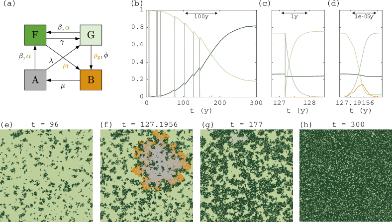
Figure 1: The FGBA stochastic cellular automaton: (a) state transition diagram (coloured rates: spread to neighbouring cell, black rates: spontaneous conversion within cell), (b) example time series of a simulation starting at zero tree cover, (c,d) $10^{2}$x and $10^{7}$x zoom of (b), (e-h) snapshots of a simulation at indicated times for low fire ignition rate ($\phi N{=}0.075$). The fire in (f) spreads throughout grassland in the whole domain whereas that in (g) went extinct locally because forest splits grassland in clusters (notice the area of ash near the top). Remaining parameters are shown in Table M1. Domain size: 200x200 cells.

In this work, we examine the spontaneous emergence of nonlinear dynamics and bistability of tropical forest from the patch-scale rules of forest and fire spread. We first use the cellular automaton of Hébert-Dufresne et al. Hébert-Dufresne et al. (2018) to observe the emergent structure and bistability in simulations. Next, based on the observations that forest and fire spread occur near the forest perimeter and on separated timescales, we set up a macroscopic balance equation of forest area change (Eq. 9). This enables us to analyse the emergent dynamics as a function of the relevant structure, and will show that the nonlinearity is caused by the forest geometry. Then, we derive a forest resilience indicator based on our balance equation, providing a proposed link between the geometry and resilience of tropical forest. Finally, we compare our results against mean-field approximations. This will show that the assumption of absence of spatial correlations is strongly violated, particularly near the tipping threshold of forest dieback, while mean-field models still permit accurate expressions for the spatially uncorrelated regime.

Results

The FGBA probabilistic cellular automaton

The FGBA probabilistic cellular automaton (adapted from (Hébert-Dufresne et al., 2018) – see Fig. 1 and Methods) models the stochastic dynamics of tropical vegetation and fire on a square lattice and in continuous time. The key empirical facts of tropical forest and fire dynamics captured by the FGBA automaton are: (i) fires only naturally ignite in grasslands but they can spread into forest, (ii) fires spread more easily in grassland than in forest, such that forests suppress fires, albeit imperfectly, (iii) forest dynamics occur on a strongly separated timescale from fire spread and grass regrowth.

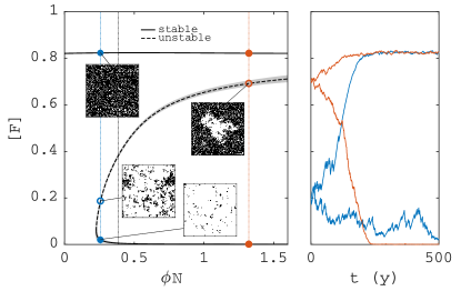
Figure 2: Steady states and bistability of forest area in the FGBA cellular automaton. (a) Bifurcation diagram of forest area fraction $\raisebox{1.07639pt}{\scalebox{0.8}{[}}\mathrm{F}\raisebox{1.07639pt}{\scalebox{0.8}{]}}$ versus fire ignition rate $\phi$ (shade: two-standard deviation confidence interval of the mean). (b) Simulations initiated at two different points on the saddle ($\phi N{=}0.257$ and $\phi N{=}1.32$). Remaining parameters are shown in Table M1. Domain size: 100x100 cells.

This results in the following reaction rules in the cellular automaton. At any time, each lattice cell can be in one of four states: $\mathrm{F}$ – forest, $\mathrm{G}$ – grass, $\mathrm{B}$ – burning, $\mathrm{A}$ – ash. Conversions between these states can occur spontaneously or due to spread to neighbouring cells (Fig. 1a and Table M1). The spontaneous conversions are: forest recruitment on grass or ash cells due to long-distance seed dispersal or from a homogeneous seed bank ($\mathrm{G}\to\mathrm{F}$ or $\mathrm{A}\to\mathrm{F}$ at rate $\beta$), forest mortality ($\mathrm{F}\to\mathrm{G}$ at rate $\gamma$), fire ignition on grass cells ($\mathrm{G}\to\mathrm{B}$ at rate $\phi$), and grass regrowth on ash cells ($\mathrm{A}\to\mathrm{G}$ at rate $\lambda$). The conversions due to spread to neighbours are: forest recruitment due to short-distance seed dispersal on grass or ash cells ($\mathrm{GF}\to\mathrm{FF},\;\mathrm{AF}\to\mathrm{FF}$ at rate $\alpha$), fire spread on grass ($\mathrm{GB}\to\mathrm{BB}$ at rate $\rho_{\mathrm{g}}$) or on tree cells ($\mathrm{FB}\to\mathrm{BB}$ at rate $\rho_{\mathrm{f}}$). Chosen parameters are in the ranges empirically justified by Hébert-Dufresne et al. (2018) for a square domain of $100$x$100$ cells, with cell size $\Delta x{=}\Delta y{=}30$m. The timescale separation between fire and forest dynamics implies that the rates satisfy $\rho_{\mathrm{g}},\rho_{\mathrm{f}},\mu,\lambda\gg\alpha,\beta,\gamma$. In particular, we choose

$$\rho_{\mathrm{g}},\mu\sim 10^{6}>\rho_{\mathrm{f}}\sim 10^{5} \gg 1\text{y}^{-1},$$ (1)

$$\alpha,\beta,\gamma\sim 10^{[-4,-2]} \ll\lambda\sim 1\text{y}^{-1}.$$ (2)

So, fire spreading and extinction $\rho_{\mathrm{g}}$, $\rho_{\mathrm{f}}$, $\mu$ occur on the scale of hours, while grass regrows on ash over months ($\lambda$) and forest spread, growth and mortality $\alpha$, $\beta$, $\gamma$ occur over decades. We take fire ignition rate $\phi\sim 1/N$ such that fires spontaneously occur about once per year in the modelled area. Figure 1b–d shows a time profile for fractions of cells in each state during a simulation with low fire ignition rate $\phi$, starting from an all-grass state. Due to the low fire ignition rate, the only stable steady state is a nearly closed canopy (reached after $300$ years, Fig. 1h). Before canopy closure, brief events of rapidly spreading fire counteract a gradual spread of forest. After canopy closure, fires are unable to spread. Timescale separation of forest dynamics (Fig. 1b), grass regrowth (Fig. 1c), and fire spread (Fig. 1d) shows clearly.

Figure 2a shows a bifurcation diagram of steady state forest area in the FGBA cellular automaton, denoted by $\raisebox{1.07639pt}{\scalebox{0.8}{[}}\mathrm{F}\raisebox{1.07639pt}{\scalebox{0.8}{]}}$ (see Eq. M1), versus fire ignition rate $\phi$. Unstable steady states (saddles) were obtained by applying feedback control to the simulations (see Methods). Bistability occurs above a critical ignition rate $\phi$, with alternative stable states grassland ($\raisebox{1.07639pt}{\scalebox{0.8}{[}}\mathrm{F}\raisebox{1.07639pt}{\scalebox{0.8}{]}}{\approx}0$) and forest ($\raisebox{1.07639pt}{\scalebox{0.8}{[}}\mathrm{F}\raisebox{1.07639pt}{\scalebox{0.8}{]}}{\approx}0.83$). Simulations initiated at the saddle will tip randomly up or down (Fig. 2b). Near the lower end of the bistability range, the saddle solution is fairly homogeneous, but for higher $\phi$ values, a single hole of grass in forest arises (insets in Fig. 2a).

Fast and slow subprocesses

The timescale separation (Eqs. 1 and 2) permits treatment of the joint vegetation and fire dynamics as a fast-slow system. Fire spread occurs on the fast timescale, where the vegetation landscape is treated as constant. Forest dynamics occur on the slow timescale, where the effects of fire are a steady state function of the vegetation landscape.

Fast process: fires spreading in a given landscape

On the timescale of a single fire event, forest dynamics are negligible ($\alpha,\beta,\gamma\ll 1/$day) such that we can consider the total landscape of forest patches as fixed. For each ignition event, this results in the following dynamics. A fire ignites on a grass cell, then spreads across its grassland cluster at a rate $\rho_{\mathrm{g}}$ per $\mathrm{BG}$ pair, after which it reaches the interface with adjacent forest, where it starts intruding the forest at a rate $\rho_{\mathrm{f}}$ per $\mathrm{BF}$ pair. At any time, a burning cell can stop burning spontaneously, converting to ash at a rate $\mu$. The probabilities of fire spreading into a neighbouring grass or forest cell before the originating cell stops burning are given by

$$p_{\mathrm{g}}:=\frac{\rho_{\mathrm{g}}}{\rho_{\mathrm{g}}+\mu}=0.9,\qquad p_{\mathrm{f}}:=\frac{\rho_{\mathrm{f}}}{\rho_{\mathrm{f}}+\mu}=0.1,$$ (3)

where we have shown the chosen values in our simulations (adopted from Hébert-Dufresne et al., 2018). Since regrowth of grass and ignition of new fires occur at a much slower rate than fire spread ($\phi N\lesssim\lambda\ll\rho_{\mathrm{f}},\mu,\rho_{\mathrm{g}}$) and our domain is relatively small (see Section S2B), we observe repeated fire spreading events well separated in time (Fig. 1b), each ending with spontaneous extinction.

When a fire in grassland cluster with index $j$ reaches its interface with adjacent forest, the resulting forest loss due to this single fire event can be approximated as (see Methods):

$$\Delta_{\mathrm{F},j}^{\mathrm{loss}}:=p_{\mathrm{f}}\raisebox{1.07639pt}{\scalebox{0.8}{[}}\mathrm{FG}\raisebox{1.07639pt}{\scalebox{0.8}{]}}_{j},$$ (4)

where $\raisebox{1.07639pt}{\scalebox{0.8}{[}}\mathrm{FG}\raisebox{1.07639pt}{\scalebox{0.8}{]}}_{j}$ counts the number of forest cells adjacent to grassland cluster $j$ (with both sides of the equation optionally normalised by $N$). This approximation relies on the assumptions that the fire reaches the whole interface with forest (i.e. $p_{\mathrm{g}}\to 1$) and only once per fire (i.e. $\rho_{\mathrm{g}}\gg\lambda\gg\phi N$), and that $p_{\mathrm{f}}$ is small.

Slow processes: forest demography and fire damage

Forest demography and loss due to repeated fires occur on the slow timescale. Writing the number of forest-grass neighbour pairs as $\raisebox{1.07639pt}{\scalebox{0.8}{[}}\mathrm{FG}\raisebox{1.07639pt}{\scalebox{0.8}{]}}$ (divided by $N$, equivalently the total perimeter of forest or grass patches, see Eq. M1), the dynamics for tree recruitment and mortality result in an expected rate of change for $\raisebox{1.07639pt}{\scalebox{0.8}{[}}\mathrm{F}\raisebox{1.07639pt}{\scalebox{0.8}{]}}$:

$$\Delta_{\mathrm{F}}^{\mathrm{gain}}:=\beta\raisebox{1.07639pt}{\scalebox{0.8}{[}}\mathrm{G}\raisebox{1.07639pt}{\scalebox{0.8}{]}}-\gamma\raisebox{1.07639pt}{\scalebox{0.8}{[}}\mathrm{F}\raisebox{1.07639pt}{\scalebox{0.8}{]}}+\alpha\raisebox{1.07639pt}{\scalebox{0.8}{[}}\mathrm{FG}\raisebox{1.07639pt}{\scalebox{0.8}{]}}.$$ (5)

In Eq. 5, the rates of change are $\beta\raisebox{1.07639pt}{\scalebox{0.8}{[}}\mathrm{G}\raisebox{1.07639pt}{\scalebox{0.8}{]}}$ for spontaneous forest growth on grass, $\gamma\raisebox{1.07639pt}{\scalebox{0.8}{[}}\mathrm{F}\raisebox{1.07639pt}{\scalebox{0.8}{]}}$ for spontaneous forest mortality, and $\alpha\raisebox{1.07639pt}{\scalebox{0.8}{[}}\mathrm{FG}\raisebox{1.07639pt}{\scalebox{0.8}{]}}$ for spread of forest into grass at its perimeter.

The rate of forest erosion at its perimeter due to fire damage over many fire events is the weighted sum over all grass clusters $j{=}1,...,n_{\mathrm{c}}$, i.e.

$$\Delta_{\mathrm{F}}^{\mathrm{loss}} :=\sum_{j=1}^{n_{\mathrm{c}}}\phi N\raisebox{1.07639pt}{\scalebox{0.8}{[}}\mathrm{G}\raisebox{1.07639pt}{\scalebox{0.8}{]}}_{j}\Delta_{\mathrm{F},j}^{\mathrm{loss}}=\phi Np_{\mathrm{f}}\sum_{j=1}^{n_{\mathrm{c}}}\raisebox{1.07639pt}{\scalebox{0.8}{[}}\mathrm{G}\raisebox{1.07639pt}{\scalebox{0.8}{]}}_{j}\raisebox{1.07639pt}{\scalebox{0.8}{[}}\mathrm{FG}\raisebox{1.07639pt}{\scalebox{0.8}{]}}_{j},$$ (6)

where $\raisebox{1.07639pt}{\scalebox{0.8}{[}}\mathrm{G}\raisebox{1.07639pt}{\scalebox{0.8}{]}}_{j}$ is the fraction of $\mathrm{G}$ cells in grass cluster $j$ (so, $\raisebox{1.07639pt}{\scalebox{0.8}{[}}\mathrm{G}\raisebox{1.07639pt}{\scalebox{0.8}{]}}{=}\sum_{j=1}^{n_{\mathrm{c}}}\raisebox{1.07639pt}{\scalebox{0.8}{[}}\mathrm{G}\raisebox{1.07639pt}{\scalebox{0.8}{]}}_{j}$), $\phi N\raisebox{1.07639pt}{\scalebox{0.8}{[}}\mathrm{G}\raisebox{1.07639pt}{\scalebox{0.8}{]}}_{j}$ is the rate at which fires spontaneously ignite in grass cluster $j$ ($\phi$ is the rate per cell and $N\raisebox{1.07639pt}{\scalebox{0.8}{[}}\mathrm{G}\raisebox{1.07639pt}{\scalebox{0.8}{]}}_{j}$ is the area of the cluster), and $\Delta_{\mathrm{F},j}^{\mathrm{loss}}{=}p_{\mathrm{f}}\raisebox{1.07639pt}{\scalebox{0.8}{[}}\mathrm{FG}\raisebox{1.07639pt}{\scalebox{0.8}{]}}_{j}$ is the conversion of forest to ash caused by each fire event (see Eq. 4) (note also that $\raisebox{1.07639pt}{\scalebox{0.8}{[}}\mathrm{FG}\raisebox{1.07639pt}{\scalebox{0.8}{]}}{=}\sum_{j=1}^{n_{\mathrm{c}}}\raisebox{1.07639pt}{\scalebox{0.8}{[}}\mathrm{FG}\raisebox{1.07639pt}{\scalebox{0.8}{]}}_{j}$). By defining the grassland-weighted forest perimeter as

$$\langle\raisebox{1.07639pt}{\scalebox{0.8}{[}}\mathrm{FG}\raisebox{1.07639pt}{\scalebox{0.8}{]}}\rangle_{\mathrm{cg}}:=\sum_{j}^{n_{\mathrm{c}}}\frac{\raisebox{1.07639pt}{\scalebox{0.8}{[}}\mathrm{G}\raisebox{1.07639pt}{\scalebox{0.8}{]}}_{j}}{\raisebox{1.07639pt}{\scalebox{0.8}{[}}\mathrm{G}\raisebox{1.07639pt}{\scalebox{0.8}{]}}}\raisebox{1.07639pt}{\scalebox{0.8}{[}}\mathrm{FG}\raisebox{1.07639pt}{\scalebox{0.8}{]}}_{j},$$ (7)

the expression for forest loss becomes

$$\Delta_{\mathrm{F}}^{\mathrm{loss}}=\phi\,p_{\mathrm{f}}\,N\raisebox{1.07639pt}{\scalebox{0.8}{[}}\mathrm{G}\raisebox{1.07639pt}{\scalebox{0.8}{]}}\langle\raisebox{1.07639pt}{\scalebox{0.8}{[}}\mathrm{FG}\raisebox{1.07639pt}{\scalebox{0.8}{]}}\rangle_{\mathrm{cg}}.$$ (8)

The grassland-weighted forest perimeter $\langle\raisebox{1.07639pt}{\scalebox{0.8}{[}}\mathrm{FG}\raisebox{1.07639pt}{\scalebox{0.8}{]}}\rangle_{\mathrm{cg}}$ is the average perimeter of forest clusters weighted by the relative size of their adjacent grass cluster.

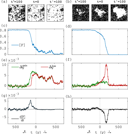
Figure 3: Rate of change according to Eq. 9. (a,b) Spatial snapshots at indicated times, (c,d) time series of $\raisebox{1.07639pt}{\scalebox{0.8}{[}}\mathrm{F}\raisebox{1.07639pt}{\scalebox{0.8}{]}}$, (e,f) time series of $\Delta_{\mathrm{F}}^{\mathrm{gain}}$, $\Delta_{\mathrm{F}}^{\mathrm{loss}}$, (g,h) time series of the right-hand side of Eq. 9 (gain minus loss). At $t{=}0$, the simulation is started on the saddle (on the left, $\raisebox{1.07639pt}{\scalebox{0.8}{[}}\mathrm{F}\raisebox{1.07639pt}{\scalebox{0.8}{]}}(0)\approx 0.2$ and on the right, $\raisebox{1.07639pt}{\scalebox{0.8}{[}}\mathrm{F}\raisebox{1.07639pt}{\scalebox{0.8}{]}}(0)\approx 0.7$, see blue and red circles in Fig. 2). Towards the left (along $t^{+}$), a simulation that tips up and towards the right (along $t^{-}$) a simulation that tips down is shown. Parameters are shown in Table M1. Columns correspond to leftmost and rightmost vertical dashed lines in Fig. 2 ($\phi N{=}0.257$ and $\phi N{=}1.32$). Domain size: 100x100 cells.

Emergent slow dynamics

We now form the balance between the slow processes discussed above, assuming fire converts trees immediately to grass (i.e. $\lambda\gg\phi N$). The resulting expected rate of forest area change during a short time interval is

$$\langle\frac{\mathrm{d}\raisebox{1.07639pt}{\scalebox{0.8}{[}}\mathrm{F}\raisebox{1.07639pt}{\scalebox{0.8}{]}}}{\mathrm{d}t}\rangle= \Delta_{\mathrm{F}}^{\mathrm{gain}}-\Delta_{\mathrm{F}}^{\mathrm{loss}},$$

$$\frac{\mathrm{d}\raisebox{1.07639pt}{\scalebox{0.8}{[}}\mathrm{F}\raisebox{1.07639pt}{\scalebox{0.8}{]}}}{\mathrm{d}t}= \beta\raisebox{1.07639pt}{\scalebox{0.8}{[}}\mathrm{G}\raisebox{1.07639pt}{\scalebox{0.8}{]}}-\gamma\raisebox{1.07639pt}{\scalebox{0.8}{[}}\mathrm{F}\raisebox{1.07639pt}{\scalebox{0.8}{]}}+\alpha\raisebox{1.07639pt}{\scalebox{0.8}{[}}\mathrm{FG}\raisebox{1.07639pt}{\scalebox{0.8}{]}}-\phi p_{\mathrm{f}}N\raisebox{1.07639pt}{\scalebox{0.8}{[}}\mathrm{G}\raisebox{1.07639pt}{\scalebox{0.8}{]}}\langle\raisebox{1.07639pt}{\scalebox{0.8}{[}}\mathrm{FG}\raisebox{1.07639pt}{\scalebox{0.8}{]}}\rangle_{\mathrm{cg}},$$ (9)

where we used Eqs. 5 and 8, and assumed on the left-hand side that $N$ is sufficiently large, such that, via the law of large numbers, $\langle\mathrm{d}\raisebox{1.07639pt}{\scalebox{0.8}{[}}\mathrm{F}\raisebox{1.07639pt}{\scalebox{0.8}{]}}/\mathrm{d}t\rangle\approx\mathrm{d}\raisebox{1.07639pt}{\scalebox{0.8}{[}}\mathrm{F}\raisebox{1.07639pt}{\scalebox{0.8}{]}}/\mathrm{d}t$. Equation 9 can be understood intuitively as forest and grass competing for space within clusters (spontaneous terms) and at their interface (interaction terms). A larger interface $\raisebox{1.07639pt}{\scalebox{0.8}{[}}\mathrm{FG}\raisebox{1.07639pt}{\scalebox{0.8}{]}}$ leads simultaneously to faster forest spread (proportional to its perimeter $\raisebox{1.07639pt}{\scalebox{0.8}{[}}\mathrm{FG}\raisebox{1.07639pt}{\scalebox{0.8}{]}}$), and to increased exposure to fires (proportional to its grassland-weighted perimeter $\langle\raisebox{1.07639pt}{\scalebox{0.8}{[}}\mathrm{FG}\raisebox{1.07639pt}{\scalebox{0.8}{]}}\rangle_{\mathrm{cg}}$). Fires are most damaging to forest when $\raisebox{1.07639pt}{\scalebox{0.8}{[}}\mathrm{G}\raisebox{1.07639pt}{\scalebox{0.8}{]}}$ forms a single cluster, i.e. $\langle\raisebox{1.07639pt}{\scalebox{0.8}{[}}\mathrm{FG}\raisebox{1.07639pt}{\scalebox{0.8}{]}}\rangle_{\mathrm{cg}}{=}\raisebox{1.07639pt}{\scalebox{0.8}{[}}\mathrm{FG}\raisebox{1.07639pt}{\scalebox{0.8}{]}}$, such that each fire reaches the whole interface. Conversely, when forest patches break $\raisebox{1.07639pt}{\scalebox{0.8}{[}}\mathrm{G}\raisebox{1.07639pt}{\scalebox{0.8}{]}}$ into several clusters $\langle\raisebox{1.07639pt}{\scalebox{0.8}{[}}\mathrm{FG}\raisebox{1.07639pt}{\scalebox{0.8}{]}}\rangle_{\mathrm{cg}}$ is smaller than $\raisebox{1.07639pt}{\scalebox{0.8}{[}}\mathrm{FG}\raisebox{1.07639pt}{\scalebox{0.8}{]}}$, such that several ignitions are required to have the same effect, slowing forest erosion down. Additionally, the total amount of grass $N\raisebox{1.07639pt}{\scalebox{0.8}{[}}\mathrm{G}\raisebox{1.07639pt}{\scalebox{0.8}{]}}$ determines the number of ignitions and hence the rate at which grass spreads into forest. The parameters determine the relative weight of each of the discussed effects.

Figure 3 shows example simulations along trajectories starting from the saddle equilibria of Fig. 2, showing forest area $\raisebox{1.07639pt}{\scalebox{0.8}{[}}\mathrm{F}\raisebox{1.07639pt}{\scalebox{0.8}{]}}$ in space and time (a–d), the gain/loss terms $\Delta_{\mathrm{F}}^{\mathrm{gain}}$ and $\Delta_{\mathrm{F}}^{\mathrm{loss}}$ defined in Eqs. 5 and 8 (e–f), and the right-hand side of Eq. 9 (gain minus loss, g–h). The left column of Fig. 3 shows simulations for low fire ignition rate $\phi$ and low $\raisebox{1.07639pt}{\scalebox{0.8}{[}}\mathrm{F}\raisebox{1.07639pt}{\scalebox{0.8}{]}}(0)$, and the right column for high $\phi$ and high $\raisebox{1.07639pt}{\scalebox{0.8}{[}}\mathrm{F}\raisebox{1.07639pt}{\scalebox{0.8}{]}}(0)$. Each column shows two realisations, both starting from the same saddle steady state. One realisation evolves toward high forest cover, shown on axis $t^{+}$ (increasing to the left from $t{=}0$), the other realisation evolves toward low forest cover, shown on axis $t^{-}$ (increasing to the right from $t{=}0$). In the stable steady states, gain (green) and loss (red) terms vary around the same mean. On the saddle (at $t{=}0$), gain and loss functions cross, indicating that the steady states and changes are accurately captured by Eq. 9. The largest changes in forest cover $\raisebox{1.07639pt}{\scalebox{0.8}{[}}\mathrm{F}\raisebox{1.07639pt}{\scalebox{0.8}{]}}$ occur when there are large changes in forest loss due to fire. The snapshots in Fig. 3a,b show that the high-cover state changes as an expanding/contracting hole in the forest, whereas the low-cover state is more homogeneous.

Emergent nonlinear relations

Equation 9 explains how the rate of change of $\raisebox{1.07639pt}{\scalebox{0.8}{[}}\mathrm{F}\raisebox{1.07639pt}{\scalebox{0.8}{]}}$ depends on the perimeter quantities $\raisebox{1.07639pt}{\scalebox{0.8}{[}}\mathrm{FG}\raisebox{1.07639pt}{\scalebox{0.8}{]}}$ and $\langle\raisebox{1.07639pt}{\scalebox{0.8}{[}}\mathrm{FG}\raisebox{1.07639pt}{\scalebox{0.8}{]}}\rangle_{\mathrm{cg}}$. Figure 4a–c shows a scatterplot of $\raisebox{1.07639pt}{\scalebox{0.8}{[}}\mathrm{FG}\raisebox{1.07639pt}{\scalebox{0.8}{]}}(t)$ and $\langle\raisebox{1.07639pt}{\scalebox{0.8}{[}}\mathrm{FG}\raisebox{1.07639pt}{\scalebox{0.8}{]}}\rangle_{\mathrm{cg}}(t)$ versus $\raisebox{1.07639pt}{\scalebox{0.8}{[}}\mathrm{F}\raisebox{1.07639pt}{\scalebox{0.8}{]}}(t)$ for three different values of $\phi$, and for an ensemble of simulations starting from the saddle in Fig. 2a, with each point being a value observed at a discrete observation time. Remarkably, we observe that $\raisebox{1.07639pt}{\scalebox{0.8}{[}}\mathrm{FG}\raisebox{1.07639pt}{\scalebox{0.8}{]}}$ and $\langle\raisebox{1.07639pt}{\scalebox{0.8}{[}}\mathrm{FG}\raisebox{1.07639pt}{\scalebox{0.8}{]}}\rangle_{\mathrm{cg}}$ lie on a narrow band around some steady state functions $\raisebox{1.07639pt}{\scalebox{0.8}{[}}\mathrm{FG}\raisebox{1.07639pt}{\scalebox{0.8}{]}}^{*}$ and $\langle\raisebox{1.07639pt}{\scalebox{0.8}{[}}\mathrm{FG}\raisebox{1.07639pt}{\scalebox{0.8}{]}}\rangle_{\mathrm{cg}}^{*}$ of $\raisebox{1.07639pt}{\scalebox{0.8}{[}}\mathrm{F}\raisebox{1.07639pt}{\scalebox{0.8}{]}}$ (and $\phi$), which implies that $\raisebox{1.07639pt}{\scalebox{0.8}{[}}\mathrm{FG}\raisebox{1.07639pt}{\scalebox{0.8}{]}},\langle\raisebox{1.07639pt}{\scalebox{0.8}{[}}\mathrm{FG}\raisebox{1.07639pt}{\scalebox{0.8}{]}}\rangle_{\mathrm{cg}}$ are changing on a much faster timescale, making them slaved to $\raisebox{1.07639pt}{\scalebox{0.8}{[}}\mathrm{F}\raisebox{1.07639pt}{\scalebox{0.8}{]}}$. Figure 4d–f shows the terms on the right-hand side of Eq. 9 depending on $\raisebox{1.07639pt}{\scalebox{0.8}{[}}\mathrm{F}\raisebox{1.07639pt}{\scalebox{0.8}{]}}$, splitting between gain and loss terms $\Delta_{\mathrm{F}}^{\mathrm{gain}},\Delta_{\mathrm{F}}^{\mathrm{loss}}$, as defined in Eqs. 5 and 8. Steady states occur when gain equals loss ($\Delta_{\mathrm{F}}^{\mathrm{gain}}{=}\Delta_{\mathrm{F}}^{\mathrm{loss}}$). The resulting plot of $\mathrm{d}\raisebox{1.07639pt}{\scalebox{0.8}{[}}\mathrm{F}\raisebox{1.07639pt}{\scalebox{0.8}{]}}/\mathrm{d}t$ versus $\raisebox{1.07639pt}{\scalebox{0.8}{[}}\mathrm{F}\raisebox{1.07639pt}{\scalebox{0.8}{]}}$ in Fig. 4g–i clearly shows the bistability of $\raisebox{1.07639pt}{\scalebox{0.8}{[}}\mathrm{F}\raisebox{1.07639pt}{\scalebox{0.8}{]}}$.

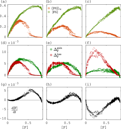
Figure 4: Emergent relations between perimeter quantities and forest area $\raisebox{1.07639pt}{\scalebox{0.8}{[}}\mathrm{F}\raisebox{1.07639pt}{\scalebox{0.8}{]}}$: (a–c) forest perimeter $\raisebox{1.07639pt}{\scalebox{0.8}{[}}\mathrm{FG}\raisebox{1.07639pt}{\scalebox{0.8}{]}}$ and grassland-weighted forest perimeter $\langle\raisebox{1.07639pt}{\scalebox{0.8}{[}}\mathrm{FG}\raisebox{1.07639pt}{\scalebox{0.8}{]}}\rangle_{\mathrm{cg}}$, (d–f) forest gain terms and loss terms in Eqs. 5 and 8, (g–i) forest area rate of change $(\mathrm{d}/\mathrm{d}t)\raisebox{1.07639pt}{\scalebox{0.8}{[}}\mathrm{F}\raisebox{1.07639pt}{\scalebox{0.8}{]}}$ from Eq. 9. Columns correspond to vertical dashed lines in Fig. 2 ($\phi N{=}0.257,\phi N{=}0.38,\phi N{=}1.32$). Domain size: 100x100 cells.

Replacing the quantities $\raisebox{1.07639pt}{\scalebox{0.8}{[}}\mathrm{FG}\raisebox{1.07639pt}{\scalebox{0.8}{]}}$ and $\langle\raisebox{1.07639pt}{\scalebox{0.8}{[}}\mathrm{FG}\raisebox{1.07639pt}{\scalebox{0.8}{]}}\rangle_{\mathrm{cg}}$ by their steady-state functions $\raisebox{1.07639pt}{\scalebox{0.8}{[}}\mathrm{FG}\raisebox{1.07639pt}{\scalebox{0.8}{]}}^{*}$ and $\langle\raisebox{1.07639pt}{\scalebox{0.8}{[}}\mathrm{FG}\raisebox{1.07639pt}{\scalebox{0.8}{]}}\rangle_{\mathrm{cg}}^{*}$ results in the single-variable ODE for $\raisebox{1.07639pt}{\scalebox{0.8}{[}}\mathrm{F}\raisebox{1.07639pt}{\scalebox{0.8}{]}}$,

$$\frac{\mathrm{d}\raisebox{1.07639pt}{\scalebox{0.8}{[}}\mathrm{F}\raisebox{1.07639pt}{\scalebox{0.8}{]}}}{\mathrm{d}t}=\beta\raisebox{1.07639pt}{\scalebox{0.8}{[}}\mathrm{G}\raisebox{1.07639pt}{\scalebox{0.8}{]}}-\gamma\raisebox{1.07639pt}{\scalebox{0.8}{[}}\mathrm{F}\raisebox{1.07639pt}{\scalebox{0.8}{]}}+\alpha\raisebox{1.07639pt}{\scalebox{0.8}{[}}\mathrm{FG}\raisebox{1.07639pt}{\scalebox{0.8}{]}}^{*}-\phi p_{\mathrm{f}}N\raisebox{1.07639pt}{\scalebox{0.8}{[}}\mathrm{G}\raisebox{1.07639pt}{\scalebox{0.8}{]}}\langle\raisebox{1.07639pt}{\scalebox{0.8}{[}}\mathrm{FG}\raisebox{1.07639pt}{\scalebox{0.8}{]}}\rangle_{\mathrm{cg}}^{*},$$ (10)

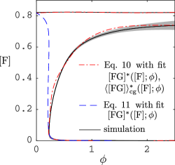
Figure S1: Steady states of Eq. 10 (multicluster – dot-dashed red) and of Eq. 11 (single cluster – dashed blue) compared to controlled simulations (solid black with shading indicating two-standard deviation confidence interval of the mean). Parameters in the cellular automaton: $\gamma{=}0.02,\alpha{=}0.03,\beta{=}2\cdot 10^{-4},\rho_{\mathrm{g}}{=}9\cdot 10^{6},\rho_{\mathrm{f}}{=}1.11\cdot 10^{5},\mu{=}10^{6},\lambda{=}5$.

where $\raisebox{1.07639pt}{\scalebox{0.8}{[}}\mathrm{FG}\raisebox{1.07639pt}{\scalebox{0.8}{]}}^{*},\langle\raisebox{1.07639pt}{\scalebox{0.8}{[}}\mathrm{FG}\raisebox{1.07639pt}{\scalebox{0.8}{]}}\rangle_{\mathrm{cg}}^{*}$ are functions of $\raisebox{1.07639pt}{\scalebox{0.8}{[}}\mathrm{F}\raisebox{1.07639pt}{\scalebox{0.8}{]}}$ and $\phi$ (as shown in Fig. 4a-c), and $\raisebox{1.07639pt}{\scalebox{0.8}{[}}\mathrm{G}\raisebox{1.07639pt}{\scalebox{0.8}{]}}{=}1-\raisebox{1.07639pt}{\scalebox{0.8}{[}}\mathrm{F}\raisebox{1.07639pt}{\scalebox{0.8}{]}}$. With these functions $\raisebox{1.07639pt}{\scalebox{0.8}{[}}\mathrm{FG}\raisebox{1.07639pt}{\scalebox{0.8}{]}}^{*}$ and $\langle\raisebox{1.07639pt}{\scalebox{0.8}{[}}\mathrm{FG}\raisebox{1.07639pt}{\scalebox{0.8}{]}}\rangle_{\mathrm{cg}}^{*}$, the observed bistability is caused by a classic double-well potential of the gradient system Eq. 10. In this ODE, nonlinearities emerge due to the equilibrium dependence of the interface on forest area (affecting $\raisebox{1.07639pt}{\scalebox{0.8}{[}}\mathrm{FG}\raisebox{1.07639pt}{\scalebox{0.8}{]}}^{*}$ and $\langle\raisebox{1.07639pt}{\scalebox{0.8}{[}}\mathrm{FG}\raisebox{1.07639pt}{\scalebox{0.8}{]}}\rangle_{\mathrm{cg}}^{*}$), due to the segmentation of grass cells near and below the percolation threshold (affecting $\langle\raisebox{1.07639pt}{\scalebox{0.8}{[}}\mathrm{FG}\raisebox{1.07639pt}{\scalebox{0.8}{]}}\rangle_{\mathrm{cg}}^{*}$) and due to dependence of the ignition rate on grass patch size (multiplying $\langle\raisebox{1.07639pt}{\scalebox{0.8}{[}}\mathrm{FG}\raisebox{1.07639pt}{\scalebox{0.8}{]}}\rangle_{\mathrm{cg}}^{*}$ with $\raisebox{1.07639pt}{\scalebox{0.8}{[}}\mathrm{G}\raisebox{1.07639pt}{\scalebox{0.8}{]}}$). In Fig. S1, we show the roots of Eq. 10 using a nonparameteric fit of $\raisebox{1.07639pt}{\scalebox{0.8}{[}}\mathrm{FG}\raisebox{1.07639pt}{\scalebox{0.8}{]}}^{*}(\raisebox{1.07639pt}{\scalebox{0.8}{[}}\mathrm{F}\raisebox{1.07639pt}{\scalebox{0.8}{]}};\phi)$ and $\langle\raisebox{1.07639pt}{\scalebox{0.8}{[}}\mathrm{FG}\raisebox{1.07639pt}{\scalebox{0.8}{]}}\rangle_{\mathrm{cg}}^{*}(\raisebox{1.07639pt}{\scalebox{0.8}{[}}\mathrm{F}\raisebox{1.07639pt}{\scalebox{0.8}{]}};\phi)$. These match well with the steady states obtained via control (dot-dashed red).

If there is only one connected component of grass cells, we have $\langle\raisebox{1.07639pt}{\scalebox{0.8}{[}}\mathrm{FG}\raisebox{1.07639pt}{\scalebox{0.8}{]}}\rangle_{\mathrm{cg}}{=}\raisebox{1.07639pt}{\scalebox{0.8}{[}}\mathrm{FG}\raisebox{1.07639pt}{\scalebox{0.8}{]}}$, such that Eq. 10 simplifies to

$$\frac{\mathrm{d}\raisebox{1.07639pt}{\scalebox{0.8}{[}}\mathrm{F}\raisebox{1.07639pt}{\scalebox{0.8}{]}}}{\mathrm{d}t}=\beta\raisebox{1.07639pt}{\scalebox{0.8}{[}}\mathrm{G}\raisebox{1.07639pt}{\scalebox{0.8}{]}}-\gamma\raisebox{1.07639pt}{\scalebox{0.8}{[}}\mathrm{F}\raisebox{1.07639pt}{\scalebox{0.8}{]}}+(\alpha-\phi p_{\mathrm{f}}N\raisebox{1.07639pt}{\scalebox{0.8}{[}}\mathrm{G}\raisebox{1.07639pt}{\scalebox{0.8}{]}})\raisebox{1.07639pt}{\scalebox{0.8}{[}}\mathrm{FG}\raisebox{1.07639pt}{\scalebox{0.8}{]}}^{*}.$$ (11)

For homogeneous initial conditions (i.e. $\raisebox{1.07639pt}{\scalebox{0.8}{[}}\mathrm{F}\raisebox{1.07639pt}{\scalebox{0.8}{]}}$ is about the same in different large subsections of the domain), this approximation is expected to be valid for small $\raisebox{1.07639pt}{\scalebox{0.8}{[}}\mathrm{F}\raisebox{1.07639pt}{\scalebox{0.8}{]}}$, where most grass cells belong to the giant connected component. Figure S1 shows the resulting steady states of Eq. 11 as a function of $\phi$ and $\raisebox{1.07639pt}{\scalebox{0.8}{[}}\mathrm{F}\raisebox{1.07639pt}{\scalebox{0.8}{]}}$ when only using the fit of $\raisebox{1.07639pt}{\scalebox{0.8}{[}}\mathrm{FG}\raisebox{1.07639pt}{\scalebox{0.8}{]}}^{*}(\raisebox{1.07639pt}{\scalebox{0.8}{[}}\mathrm{F}\raisebox{1.07639pt}{\scalebox{0.8}{]}};\phi)$ (dashed blue). The approximation is good for landscapes with low forest cover ($\raisebox{1.07639pt}{\scalebox{0.8}{[}}\mathrm{F}\raisebox{1.07639pt}{\scalebox{0.8}{]}}\lesssim 0.2$). Above $\raisebox{1.07639pt}{\scalebox{0.8}{[}}\mathrm{F}\raisebox{1.07639pt}{\scalebox{0.8}{]}}\approx 0.2$, it fails because the grassland breaks up into multiple clusters and fires are smaller than in case of a single cluster. Figure 4a–c already indicated that the single-cluster approximation is accurate for low forest cover since $\langle\raisebox{1.07639pt}{\scalebox{0.8}{[}}\mathrm{FG}\raisebox{1.07639pt}{\scalebox{0.8}{]}}\rangle_{\mathrm{cg}}{\approx}\raisebox{1.07639pt}{\scalebox{0.8}{[}}\mathrm{FG}\raisebox{1.07639pt}{\scalebox{0.8}{]}}$ for low $\raisebox{1.07639pt}{\scalebox{0.8}{[}}\mathrm{F}\raisebox{1.07639pt}{\scalebox{0.8}{]}}$ in the scatterplots.

Resilience to perturbations

One can evaluate the right-hand side of Eq. 9 for a landscape before and after application of a small perturbation, to determine if the perturbation will be dampened or amplified under the dynamics. More precisely, we may define the sensitivity as

$$\lambda_{\mathrm{F}}(X,\delta X):=\frac{\Delta\dot{\raisebox{1.07639pt}{\scalebox{0.8}{[}}\mathrm{F}\raisebox{1.07639pt}{\scalebox{0.8}{]}}}(X,\delta X)}{\Delta\raisebox{1.07639pt}{\scalebox{0.8}{[}}\mathrm{F}\raisebox{1.07639pt}{\scalebox{0.8}{]}}(X,\delta X)}=\frac{\dot{\raisebox{1.07639pt}{\scalebox{0.8}{[}}\mathrm{F}\raisebox{1.07639pt}{\scalebox{0.8}{]}}}(X+\delta X)-\dot{\raisebox{1.07639pt}{\scalebox{0.8}{[}}\mathrm{F}\raisebox{1.07639pt}{\scalebox{0.8}{]}}}(X)}{\raisebox{1.07639pt}{\scalebox{0.8}{[}}\mathrm{F}\raisebox{1.07639pt}{\scalebox{0.8}{]}}(X+\delta X)-\raisebox{1.07639pt}{\scalebox{0.8}{[}}\mathrm{F}\raisebox{1.07639pt}{\scalebox{0.8}{]}}(X)},$$ (12)

for a landscape $X$ and a perturbation $\delta X$, where $\dot{\raisebox{1.07639pt}{\scalebox{0.8}{[}}\mathrm{F}\raisebox{1.07639pt}{\scalebox{0.8}{]}}}$ is the right-hand side of Eq. 9. Negative values of $\lambda_{\mathrm{F}}$ correspond to dampening (negative feedback) and positive values to amplification (positive feedback). Given that the dynamics of Eq. 9 are an approximate function of $\raisebox{1.07639pt}{\scalebox{0.8}{[}}\mathrm{F}\raisebox{1.07639pt}{\scalebox{0.8}{]}}$ only, the average of $\lambda_{\mathrm{F}}(X{+}\delta X)$ over naturally expected perturbations $\delta X$ (call this $\bar{\lambda}_{\mathrm{F}}(X)$; see Methods, Eq. M9) can be interpreted as the approximate derivative $\mathrm{d}\dot{\raisebox{1.07639pt}{\scalebox{0.8}{[}}\mathrm{F}\raisebox{1.07639pt}{\scalebox{0.8}{]}}}(\raisebox{1.07639pt}{\scalebox{0.8}{[}}\mathrm{F}\raisebox{1.07639pt}{\scalebox{0.8}{]}})/\mathrm{d}\raisebox{1.07639pt}{\scalebox{0.8}{[}}\mathrm{F}\raisebox{1.07639pt}{\scalebox{0.8}{]}}$, which fully characterises the local stability of the landscape. Therefore, the sign and magnitude of $\bar{\lambda}_{\mathrm{F}}(X)$ are indicators for the stability or criticality of a landscape. The dependence on only $\raisebox{1.07639pt}{\scalebox{0.8}{[}}\mathrm{F}\raisebox{1.07639pt}{\scalebox{0.8}{]}}$ also implies that Eq. 9 is a gradient system, such that $\bar{\lambda}_{\mathrm{F}}(X)$ is the concavity of the potential energy function at $X$, corresponding to the classic potential-well metaphor of local resilience Scheffer et al. (2009, 2015).

Figure 5d shows $\bar{\lambda}_{\mathrm{F}}(X)$ for the traversed landscapes when tipping up to the forest or down to the grassland state (same landscapes as in Fig. 3b,d,f,g). Comparison of the magnitude of $\bar{\lambda}_{\mathrm{F}}(X)$ in the alternative stable states reveals that (for parameters of Fig. 3d,f,g) the grassland state is more resilient than the forest state. Figure 5a–c shows the positive feedback for a forest landscape with a hole of critical size (same landscape as shown at $t{=}0$ in Fig. 3b). Panel b shows which cells along the perimeter of the largest grass cluster contribute to the loss term $\Delta_{\mathrm{F}}^{\mathrm{loss}}$ (red) and the gain term $\Delta_{\mathrm{F}}^{\mathrm{gain}}$ (green). Panel a shows the effect of the perturbation obtained by converting the green cells to forest, which causes an increase in $\dot{\raisebox{1.07639pt}{\scalebox{0.8}{[}}\mathrm{F}\raisebox{1.07639pt}{\scalebox{0.8}{]}}}$ (more green in panel a). Panel c shows the effect of the perturbation converting the red cells to grass, which causes a decrease in $\dot{\raisebox{1.07639pt}{\scalebox{0.8}{[}}\mathrm{F}\raisebox{1.07639pt}{\scalebox{0.8}{]}}}$ (more red in panel c), illustrating the spatial distribution of the positive feedback.

One could, in principle, also test the effect of large perturbations, and whether they will induce a transition to an alternative stable state, but it is not in general clear which perturbations are to be expected. However, in the special case of $\beta{=}\gamma{=}0$, when the large perturbation is a single hole in contiguous forest, only the size of the hole matters, and a simple expression for the critical size required to tip abruptly to a non-forest state can be derived (see Methods, Eq. M8).

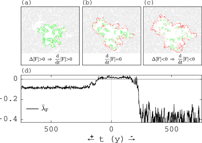
Figure 5: Resilience of forest-grass landscape to perturbations. (a–c) Spatially resolved contributions to forest gain (green) and loss (red) rates at the forest perimeter of the largest grass cluster: (b) for the saddle solution (where $\Delta_{\mathrm{F}}^{\mathrm{gain}}{\approx}\Delta_{\mathrm{F}}^{\mathrm{loss}}$), (a) for a perturbation of the saddle with more forest at the perimeter (resulting in $\Delta_{\mathrm{F}}^{\mathrm{gain}}{>}\Delta_{\mathrm{F}}^{\mathrm{loss}}$), and (c) for a perturbation of the saddle with less forest at the perimeter (resulting in $\Delta_{\mathrm{F}}^{\mathrm{loss}}{>}\Delta_{\mathrm{F}}^{\mathrm{gain}}$). (d) Sensitivity to perturbations (Eq. 12) for all the traversed landscapes when tipping from the saddle: down to the grassland state ($t^{-}$), or, up to the forest state ($t^{+}$). The used landscapes correspond to the red vertical dashed line in Fig. 2 and the rightmost columns in Figs. 3 and 4.

Comparison to mean-field approximations

Our analysis of Eq. 9 enabled us to obtain macroscopic steady states and dynamics without making mean-field assumptions. Sections S3 and S3 derive a hierarchy of mean-field models for which we compare their predictions to our results to examine their validity. The simple mean field (Section S3) is unable to capture repeated fire extinction on a fast timescale and nearest-neighbour spreading of forest and fire, leading to severe bias. When instead assuming timescale separation between forest and fire dynamics and treating fire as a site percolation process in landscapes with uniform random (i.e., spatially uncorrelated) placement of forest, we obtain the mean-field approximation of Eq. 9:

$$\frac{\mathrm{d}}{\mathrm{d}t}\raisebox{1.07639pt}{\scalebox{0.8}{[}}\mathrm{F}\raisebox{1.07639pt}{\scalebox{0.8}{]}} =\beta\raisebox{1.07639pt}{\scalebox{0.8}{[}}\mathrm{G}\raisebox{1.07639pt}{\scalebox{0.8}{]}}+4\alpha\raisebox{1.07639pt}{\scalebox{0.8}{[}}\mathrm{F}\raisebox{1.07639pt}{\scalebox{0.8}{]}}\raisebox{1.07639pt}{\scalebox{0.8}{[}}\mathrm{G}\raisebox{1.07639pt}{\scalebox{0.8}{]}}-\gamma\raisebox{1.07639pt}{\scalebox{0.8}{[}}\mathrm{F}\raisebox{1.07639pt}{\scalebox{0.8}{]}}-\phi Np_{\mathrm{f}}\raisebox{1.07639pt}{\scalebox{0.8}{[}}\mathrm{G}\raisebox{1.07639pt}{\scalebox{0.8}{]}}\langle\raisebox{1.07639pt}{\scalebox{0.8}{[}}\mathrm{FG}\raisebox{1.07639pt}{\scalebox{0.8}{]}}\rangle_{\mathrm{cg}}^{\mathrm{u}}.$$ (13)

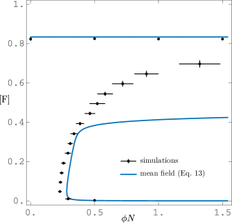
Figure S2: Comparison of steady state forest as a function of ignition rate in the time-separated mean-field and in simulations (dots with error bars: simulations, lines: mean field). A large difference between mean-field model and simulation occurs for the threshold steady state, while the mean-field model is accurate for high- and low-tree-cover alternative stable states. See Section S4S4.2 and Fig. S9 for comparison of other scenarios and mean-field approximations.

In Eq. 13 we substituted the a-priori unknown forest perimeter $\raisebox{1.07639pt}{\scalebox{0.8}{[}}\mathrm{FG}\raisebox{1.07639pt}{\scalebox{0.8}{]}}$ and the grassland-weighted perimeter $\langle\raisebox{1.07639pt}{\scalebox{0.8}{[}}\mathrm{FG}\raisebox{1.07639pt}{\scalebox{0.8}{]}}\rangle_{\mathrm{cg}}$ by their expressions assuming absence of correlations: $\raisebox{1.07639pt}{\scalebox{0.8}{[}}\mathrm{FG}\raisebox{1.07639pt}{\scalebox{0.8}{]}}{\approx}4\raisebox{1.07639pt}{\scalebox{0.8}{[}}\mathrm{F}\raisebox{1.07639pt}{\scalebox{0.8}{]}}\raisebox{1.07639pt}{\scalebox{0.8}{[}}\mathrm{G}\raisebox{1.07639pt}{\scalebox{0.8}{]}}$ and $\langle\raisebox{1.07639pt}{\scalebox{0.8}{[}}\mathrm{FG}\raisebox{1.07639pt}{\scalebox{0.8}{]}}\rangle_{\mathrm{cg}}{\approx}\langle\raisebox{1.07639pt}{\scalebox{0.8}{[}}\mathrm{FG}\raisebox{1.07639pt}{\scalebox{0.8}{]}}\rangle_{\mathrm{cg}}^{\mathrm{u}}$ for given $\raisebox{1.07639pt}{\scalebox{0.8}{[}}\mathrm{F}\raisebox{1.07639pt}{\scalebox{0.8}{]}}$. The function $\langle\raisebox{1.07639pt}{\scalebox{0.8}{[}}\mathrm{FG}\raisebox{1.07639pt}{\scalebox{0.8}{]}}\rangle_{\mathrm{cg}}^{\mathrm{u}}(\raisebox{1.07639pt}{\scalebox{0.8}{[}}\mathrm{F}\raisebox{1.07639pt}{\scalebox{0.8}{]}})$ is the quantity given in Eq. 7 for uniformly randomly placed forest (see orange curve in Fig. S3a-c). Eq. 13 is bistable with stable high and low forest cover steady states over a wide range of parameters. It accurately predicts the location of both stable steady states (blue line in Fig. S2). Yet, its prediction of the threshold (unstable) steady state and the dynamics remains strongly biased. Indeed, away from the stable steady states, the interplay of forest demography and fire-induced forest erosion creates landscapes in which forest is spatially aggregated, strongly violating the assumption of absence of correlations. This can be seen in Fig. S3a–c. which shows that for given forest area $\raisebox{1.07639pt}{\scalebox{0.8}{[}}\mathrm{F}\raisebox{1.07639pt}{\scalebox{0.8}{]}}$, the forest perimeter of simulations, $\raisebox{1.07639pt}{\scalebox{0.8}{[}}\mathrm{FG}\raisebox{1.07639pt}{\scalebox{0.8}{]}}$, lies below that predicted by the mean-field, $\raisebox{1.07639pt}{\scalebox{0.8}{[}}\mathrm{FG}\raisebox{1.07639pt}{\scalebox{0.8}{]}}_{\mathrm{mf}}$, i.e.

$$\raisebox{1.07639pt}{\scalebox{0.8}{[}}\mathrm{FG}\raisebox{1.07639pt}{\scalebox{0.8}{]}}<\raisebox{1.07639pt}{\scalebox{0.8}{[}}\mathrm{FG}\raisebox{1.07639pt}{\scalebox{0.8}{]}}_{\mathrm{mf}}=4\raisebox{1.07639pt}{\scalebox{0.8}{[}}\mathrm{F}\raisebox{1.07639pt}{\scalebox{0.8}{]}}(1-\raisebox{1.07639pt}{\scalebox{0.8}{[}}\mathrm{F}\raisebox{1.07639pt}{\scalebox{0.8}{]}}),$$ (14)

implying that forest is more spatially aggregated than assumed in the mean field. Aggregation results from forest spreading close to existing forest and from lower survival of forest cells that are more exposed to fire (i.e., less aggregated). Forest gain is smaller when aggregated (Fig. S3d–f) due to the smaller perimeter. Aggregation reduces forest loss at low cover while it increases forest loss at high cover (Fig. S3d–f). This is so because aggregation makes forest cells individually less exposed to fire, but collectively less effective at blocking fires, where the individual effect is dominant at low cover and the collective effect is dominant at cover values near and above the fire percolation threshold.

For our choice of parameters, the stable steady states and the lower saddle-node bifurcation contain negligible spatial structure, such that mean-field predictions are accurate. We derive their expressions below for $\beta{\approx}0$ .

Stable steady states

By Eq. 13, the low-cover steady state $\raisebox{1.07639pt}{\scalebox{0.8}{[}}\mathrm{F}\raisebox{1.07639pt}{\scalebox{0.8}{]}}^{*}_{-}$ has to be approximately zero for $\beta{\approx}0$. At high forest cover, loss due to fire is negligible, such that the high-cover steady state $\raisebox{1.07639pt}{\scalebox{0.8}{[}}\mathrm{F}\raisebox{1.07639pt}{\scalebox{0.8}{]}}^{*}_{+}$ can also be obtained from Eq. 13 (using $\beta{\approx}0$):

$$\raisebox{1.07639pt}{\scalebox{0.8}{[}}\mathrm{F}\raisebox{1.07639pt}{\scalebox{0.8}{]}}^{*}_{-}=0,\qquad\raisebox{1.07639pt}{\scalebox{0.8}{[}}\mathrm{F}\raisebox{1.07639pt}{\scalebox{0.8}{]}}^{*}_{+}=1-\frac{\gamma}{4\alpha}.$$ (15)

For the chosen parameters, we have $\raisebox{1.07639pt}{\scalebox{0.8}{[}}\mathrm{F}\raisebox{1.07639pt}{\scalebox{0.8}{]}}^{*}_{+}{=}0.83$, which is in excellent agreement with simulations (Fig. 2).

Onset of bistability

At low forest cover, grass consists of a single cluster, such that we can write in Eq. 13 $\langle\raisebox{1.07639pt}{\scalebox{0.8}{[}}\mathrm{FG}\raisebox{1.07639pt}{\scalebox{0.8}{]}}\rangle_{\mathrm{cg}}^{\mathrm{u}}{=}\raisebox{1.07639pt}{\scalebox{0.8}{[}}\mathrm{FG}\raisebox{1.07639pt}{\scalebox{0.8}{]}}{=}4\raisebox{1.07639pt}{\scalebox{0.8}{[}}\mathrm{F}\raisebox{1.07639pt}{\scalebox{0.8}{]}}\raisebox{1.07639pt}{\scalebox{0.8}{[}}\mathrm{G}\raisebox{1.07639pt}{\scalebox{0.8}{]}}$. Hence (when $\beta{\approx}0$):

$$\frac{\mathrm{d}}{\mathrm{d}t}\raisebox{1.07639pt}{\scalebox{0.8}{[}}\mathrm{F}\raisebox{1.07639pt}{\scalebox{0.8}{]}}=4\alpha\raisebox{1.07639pt}{\scalebox{0.8}{[}}\mathrm{F}\raisebox{1.07639pt}{\scalebox{0.8}{]}}\raisebox{1.07639pt}{\scalebox{0.8}{[}}\mathrm{G}\raisebox{1.07639pt}{\scalebox{0.8}{]}}-\gamma\raisebox{1.07639pt}{\scalebox{0.8}{[}}\mathrm{F}\raisebox{1.07639pt}{\scalebox{0.8}{]}}-4\phi Np_{\mathrm{f}}\raisebox{1.07639pt}{\scalebox{0.8}{[}}\mathrm{G}\raisebox{1.07639pt}{\scalebox{0.8}{]}}^{2}\raisebox{1.07639pt}{\scalebox{0.8}{[}}\mathrm{F}\raisebox{1.07639pt}{\scalebox{0.8}{]}}.$$ (16)

An expression for the lower bifurcation point can be obtained by finding the root of the derivative of the right-hand side of Eq. 16 with respect to $\raisebox{1.07639pt}{\scalebox{0.8}{[}}\mathrm{F}\raisebox{1.07639pt}{\scalebox{0.8}{]}}$ at $\raisebox{1.07639pt}{\scalebox{0.8}{[}}\mathrm{F}\raisebox{1.07639pt}{\scalebox{0.8}{]}}{=}\raisebox{1.07639pt}{\scalebox{0.8}{[}}\mathrm{F}\raisebox{1.07639pt}{\scalebox{0.8}{]}}^{*}_{-}{=}0$, giving the relation $4\alpha-\gamma-4\phi Np_{\mathrm{f}}=0$. Rearranging this relation for $\phi N$, we can obtain the fire ignition rate above which tropical forests are bistable with grasslands:

$$(\phi N)_{\mathrm{min}}=\frac{1}{p_{\mathrm{f}}}(\alpha-\frac{\gamma}{4}).$$ (17)

For the chosen parameters, $(\phi N)_{\mathrm{min}}{=}0.25$, which agrees well with simulations (Fig. 2) and which corresponds to a maximum fire return interval of $(\phi N)_{\mathrm{min}}^{-1}{=}4\mathrm{y}$.

Discussion

In this paper, we showed how nonlinear dynamics and bistability of tropical forest emerge spontaneously from the patch-scale rules of forest and fire spread, without assuming equations or thresholds for the effects of fire as in previous work. Below, we first summarise our main results on structure and dynamics. Then we discuss the importance of the emergent structure as indicated by comparison with mean-field approximations. Finally, we highlight the potential practical implications of our results for resilience assessment and conservation.

Emergent structure and dynamics

Our simulations showed that spatial structure emerges due to forest expansion and fire-induced damage at the forest perimeter. As a consequence, the forest perimeter appeared in both the gain and loss side of our landscape-scale balance equation of forest area, Eq. 9, where losses require weighting by adjacent grassland area. Remarkably, when plotting the changes predicted by our balance equation versus forest area, using landscapes from the simulations, we found that they lie on an approximate curve (Fig. 4g–h). As this curve shows the change of forest area as a function of forest area, this means that the emergent macroscopic dynamics can be described by a simple ordinary differential equation, Eq. 10. In this emergent closed form of our balance equation, the perimeter quantities determine the nonlinearities. Therefore, Eq. 10 elucidates how forest dynamics and bistability are linked to the forest geometry that emerges from the patch-scale spreading rules. Note that, as in previous work, Eq. 10 does not include fire explicitly, because it does not contain equations for fire. This follows from timescale separation between fire and vegetation dynamics, an assumption that was already implicit in mean-field models (Staver and Levin, 2012; Touboul et al., 2018; Li et al., 2019; Wuyts et al., 2019; Goel et al., 2020; mean field in Schertzer et al., 2014; Patterson et al., 2021) and microscopic models (microscopic models in Schertzer et al., 2014; Patterson et al., 2021) focusing on alternative stable states. However, previous work derived the implicit effect of fire in closed form by relying on standard percolation theory, which assumes that occurrence of flammable patches is spatially uncorrelated Stauffer and Aharony (1994). As we did not rely on percolation theory, but observed the closed form emerging in simulations (Fig. 4), we could avoid the biases that affect previous work.

Evaluation of mean-field models

We compared mean-field models against the emergent closed form of our balance equation to assess their validity (Fig. S3) and to show where spatial structure is important. This showed that mean-field models are in qualitative but not quantitative agreement with simulations: existence of bistability, but not its parameter range is robust to mean-field assumptions. In particular, the simple mean field (Eq. S7) is strongly biased due to its failure to account for two phenomena that are present in the microscale model: (i) spontaneous fire extinction on the fast timescale, leading to separated rapid fire spreading events, (ii) nearest-neighbour spreading of fire and forest, leading to emergent aggregation of forest patches away from the steady states. The former violates the mean-field assumption of large system size ($N{\to}\infty$) and the latter that of absence of correlations. That spatial structure affects steady states and dynamics is well known (e.g. Keeling, 1999; Dieckmann et al., 2000). Even when addressing timescale separation and using results from percolation theory for the effect of fire (Eq. S18 or Eq. S22), a large bias remains except near the alternative stable states Fig. S3. This is because standard percolation theory only considers lattice configurations with uniform random (i.e., spatially uncorrelated) placement of flammable sites while our forest-grass landscapes are shaped by past fires and vegetation dynamics. As Fig. 3a,b (at $t{=}0$) shows, forest aggregation is particularly strong at the tipping threshold for forest collapse, implying that mean-field models cannot be used to study abrupt forest dieback. Despite their severe bias concerning forest dynamics and tipping, mean-field models are still useful for studying regimes with little structure, such as near the stable equilibria or for dynamics with uniform seed dispersal. This enabled us to derive expressions for these equilibria (Eq. 15) and the point of onset of bistability (Eq. 17). The latter result was not obtained by previous mean-field models because they did not include parameters that relate directly to fire (Schertzer et al., 2014; Staver and Levin, 2012, see Section S7 for a suggested modification) or they did not account for timescale separation in finite domains Hébert-Dufresne et al. (2018).

Implications for resilience assessment and conservation

The link between geometry and dynamics implies that tropical forest resilience can be empirically estimated from its spatial structure. The spatial structure, as captured by the perimeter quantities $\raisebox{1.07639pt}{\scalebox{0.8}{[}}\mathrm{FG}\raisebox{1.07639pt}{\scalebox{0.8}{]}}$ and $\langle\raisebox{1.07639pt}{\scalebox{0.8}{[}}\mathrm{FG}\raisebox{1.07639pt}{\scalebox{0.8}{]}}\rangle_{\mathrm{cg}}$, can hence be treated as a measurable parameter additional to the microscopic parameters. Microscopic parameters (given in Table M1) can be inferred from remote-sensed data (as in Hébert-Dufresne et al., 2018 or Aleman and Staver, 2018) or from experiments (as for fire spread in Cardoso et al., 2022), while the perimeter quantities can be calculated for any observed landscape. In regimes with negligible spatial structure, one can assess stability or resilience from the microscopic parameters alone, based on mean-field results. E.g., if the onset point of bistability at low tree cover lies in the regime without spatial structure, as in our simulations, one can directly estimate the minimum fire ignition rate for onset of bistability from the microscopic parameters (Eq. 17). This expression then shows which natural or abandoned degraded areas of low tree cover with fire ignition rate beyond this point will not spontaneously recover to closed tropical forest. In regimes with spatial structure, the mean field is highly inaccurate (Fig. S3), such that spatial structure needs to be considered in addition to the parameters. In particular, in our simulations, the tipping threshold obtains spatial structure at higher fire ignition rates (Fig. 3a,b at $t{=}0$) and approaches the stable forest equilibrium much more closely than in the mean field (Fig. S2). While this makes the mean field unsuitable for studying forest resilience and dieback, our balance equation (Eq. 9) does not have this limitation because it makes no assumption on spatial structure. We demonstrated how Eq. 9 permits estimation of the resilience of a landscape to perturbations, via $\lambda_{\mathrm{F}}$ (Eq. 12). In contrast to generic indicators of resilience Scheffer et al. (2009); Boulton et al. (2022), $\lambda_{\mathrm{F}}$ is an indicator that can be obtained from a single landscape, and for which the contribution of each relevant spatial process can be examined. Furthermore, landscape perturbations by human intervention can be evaluated, through sensitivity $\lambda_{\mathrm{F}}$, for how they will amplify or mitigate fire-vegetation feedback. Forest conservation/restoration may introduce targeted perturbations that most efficiently prevent resilience loss of high-cover states or induce resilience loss of low-cover states. For instance, in Fig. 5a, forest dieback is averted by a perturbation that divides the largest grass cluster into smaller ones. It may thus be anticipated that maintenance or creation of barriers to fire spread will be essential here.

Future work could explore further realism, such as environmental heterogeneity, longer dispersal ranges, non-lattice geometry (as in Patterson et al., 2021), inclusion of other tree types (such as in savanna dynamics: Staver and Levin, 2012; Schertzer et al., 2014; Touboul et al., 2018; Van Langevelde et al., 2003; Accatino et al., 2010; D’Odorico et al., 2006; Baudena et al., 2010; Beckage et al., 2011; Hoyer-Leitzel and Iams, 2021; Patterson et al., 2021), or vegetation-rainfall feedback Spracklen et al. (2018). This may result in additional relevant quantities in Eq. 9. Additionally, larger domain sizes may lead to more gradual transitions on the macroscopic scale (Rietkerk et al., 2021, Section S6).

Methods

Details of the FGBA probabilistic cellular automaton

The FGBA probabilistic cellular automaton is a minimal spatial stochastic process that models the joint dynamics of tropical vegetation and fire. It is an adapted version of the BGT(A) model of ref. (Hébert-Dufresne et al., 2018). The modifications compared to ref. (Hébert-Dufresne et al., 2018) are: (i) it runs in continuous time, (ii) it includes a spontaneous forest mortality rate $\gamma$, (iii) species $\mathrm{T}$ is labelled as $\mathrm{F}$, consistent with other models of tropical vegetation dynamics (Staver and Levin, 2012; Wuyts et al., 2019; Patterson et al., 2021). Note that according to some definitions, probabilistic continuous-time cellular automata are considered as interacting particle systems. In general, when studying the stochastic dynamics of a number $n$ of interacting species on a square lattice with $N$ cells, the state of the system can be represented as

$$X:=(X_{1},X_{2},...,X_{N}),$$

where $X_{i}$ is the label of the species that occupies cell $i$. Each cell is occupied by exactly one of four possible species: grass, forest, burning and ash, with labels $\mathrm{G}$, $\mathrm{F}$, $\mathrm{B}$ and $\mathrm{A}$. Transitions between states (species) occur in continuous time, resulting in a continuous-time Markov chain with a state space of size $n^{N}$. The reaction rules for transitions between states are shown in Table M1, where spontaneous conversions are shown on the left and conversions due to nearest-neighbour interactions on the right (see also Fig. 1a).

Table M1: Reactions and rates (y^-1) in the CA.

	Spontaneous		Spread
forest	$\mathrm{G},\mathrm{A}\overset{\beta}{\to}\mathrm{F},$	$\beta=2\cdot 10^{-4}$	$\mathrm{GF},\mathrm{AF}\overset{\alpha}{\to}\mathrm{FF},$	$\alpha_{\;}=3\cdot 10^{-2}$
	$\mathrm{F}\overset{\gamma}{\to}\mathrm{G},$	$\gamma=2\cdot 10^{-2}$
fire	$\mathrm{G}\overset{\phi}{\to}\mathrm{B},$	$\phi=[0,2]\cdot 10^{-4}$	$\mathrm{GB}\overset{\rho_{\mathrm{g}}}{\to}\mathrm{BB},$	$\rho_{\mathrm{g}}=9\cdot 10^{6}$
	$\mathrm{B}\overset{\mu}{\to}\mathrm{A},$	$\mu=10^{6}$	$\mathrm{FB}\overset{\rho_{\mathrm{f}}}{\rightarrow}\mathrm{BB},$	$\rho_{\mathrm{f}}=1.11\cdot 10^{5}$
	$\mathrm{A}\overset{\lambda}{\to}\mathrm{G},$	$\lambda=5$

The latter type of interaction occurs over each four nearest neighbour connections of the indicated type. E.g., fire will spread into a given grass cell with a rate $\rho_{\mathrm{g}}$ for each burning neighbour. For realistic timescales, our parameters satisfy Eqs. 1 and 2, which were empirically justified in Hébert-Dufresne et al. (2018). We borrow our notation from the moment closure literature (e.g. Keeling, 1999; Dieckmann et al., 2000; Kiss et al., 2017; Wuyts and Sieber, 2022), writing the global fraction of species with label $\mathrm{x}$ and the interface between species with label $\mathrm{x}$ with label $\mathrm{y}$ respectively as

$$\raisebox{1.07639pt}{\scalebox{0.8}{[}}\mathrm{x}\raisebox{1.07639pt}{\scalebox{0.8}{]}}:=\frac{1}{N}\sum_{i}^{N}\delta_{\mathrm{x}}(X_{i}),\quad\raisebox{1.07639pt}{\scalebox{0.8}{[}}\mathrm{xy}\raisebox{1.07639pt}{\scalebox{0.8}{]}}:=\frac{1}{N}\sum_{i,j}^{N}\mathsf{A}_{ij}\delta_{\mathrm{x}}(X_{i})\delta_{\mathrm{y}}(X_{j}),$$ (M1)

where both are normalised by $N$, $\delta$ is the Kronecker delta function ($\delta_{\mathrm{x}}(y){=}1$ if $y{=}\mathrm{x}$ and $0$ otherwise) and $\mathsf{A}\in\{0,1\}^{N\times N}$ the adjacency matrix. We simulated the cellular automaton via a Gillespie algorithm (Gillespie, 2007) and used a domain of $N{=}100{\times}100$ ($N{=}200{\times}200$ in Fig. 1) cells with periodic boundary conditions.

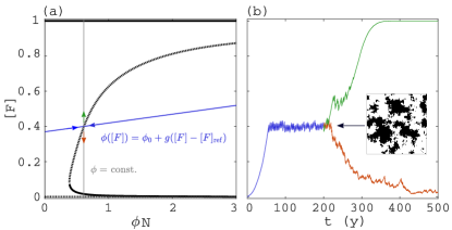
Figure M1: Feedback control applied to the CA without spontaneous mortality ($\gamma{=}0$): (a) the unstable steady state of the bifurcation diagram (dashed) was derived via feedback control by letting $\phi$ be a function of $\raisebox{1.07639pt}{\scalebox{0.8}{[}}\mathrm{F}\raisebox{1.07639pt}{\scalebox{0.8}{]}}$ (blue line) such that it is stabilised, then obtaining $(\phi,\raisebox{1.07639pt}{\scalebox{0.8}{[}}\mathrm{F}\raisebox{1.07639pt}{\scalebox{0.8}{]}})$ by averaging and repeating this for many $\raisebox{1.07639pt}{\scalebox{0.8}{[}}\mathrm{F}\raisebox{1.07639pt}{\scalebox{0.8}{]}}_{\mathrm{ref}}$ (with appropriate $g$), (b) a regular simulation with the same $\phi$ value (solid grey in (a)) and starting from the final state of the controlled simulation tips up or down depending on initial perturbations, (c) snapshot of the domain at the saddle for the control indicated in (a) (black: forest, white: grass). For other parameters, see Table M1.

Noninvasive feedback control

To study steady states regardless of their stability in a simulation, we apply noninvasive feedback control (Sieber et al., 2008; Schilder et al., 2015; Barton, 2017; Neville et al., 2018). To obtain the dependence of equilibria of $\raisebox{1.07639pt}{\scalebox{0.8}{[}}\mathrm{F}\raisebox{1.07639pt}{\scalebox{0.8}{]}}$ on fire ignition rate $\phi$, we introduced an artificial stabilizing feedback loop of the form

$$\phi(t)=\phi_{0}+g(\raisebox{1.07639pt}{\scalebox{0.8}{[}}\mathrm{F}\raisebox{1.07639pt}{\scalebox{0.8}{]}}(t)-\raisebox{1.07639pt}{\scalebox{0.8}{[}}\mathrm{F}\raisebox{1.07639pt}{\scalebox{0.8}{]}}_{\mathrm{ref}}).$$ (M2)

The factor $g$ is called the feedback control gain and is problem specific. The property of noninvasiveness means that the controlled simulations have the same equilibria as regular simulations (Barton and Sieber, 2013; Sieber et al., 2014; Renson et al., 2017). This implies that if one extracts the equilibrium values of the controlled simulation $(\phi^{*},\raisebox{1.07639pt}{\scalebox{0.8}{[}}\mathrm{F}\raisebox{1.07639pt}{\scalebox{0.8}{]}}^{*})$, one can use them to plot a 1-parameter bifurcation diagram of the simulation without control. Fig. M1 shows the control graphically. The feedback Eq. M2, indicated in blue in Fig. M1a, stabilises a steady state that is unstable in a regular simulation. This can be seen in Fig. M1b, where the unstable steady state is first stabilised via control, after which the control is removed and a regular simulation is started with the effective rate and the landscape (inset) obtained from the controlled simulation. Depending on initial perturbations, the regular simulation gets either attracted to the 100% forest state or to the low tree cover state. When the controlled simulation is in equilibrium (steady part of the blue curve in Fig. M1b), the steady state values of $\raisebox{1.07639pt}{\scalebox{0.8}{[}}\mathrm{F}\raisebox{1.07639pt}{\scalebox{0.8}{]}}$ are obtained via taking the time average, i.e.

$$\overline{\raisebox{1.07639pt}{\scalebox{0.8}{[}}\mathrm{F}\raisebox{1.07639pt}{\scalebox{0.8}{]}}}=\frac{1}{T}\int_{t_{0}}^{t_{0}+T}\raisebox{1.07639pt}{\scalebox{0.8}{[}}\mathrm{F}\raisebox{1.07639pt}{\scalebox{0.8}{]}}(t)dt,$$ (M3)

where $t_{0}$ is the time after which the dynamics have settled to a steady state and $T$ the averaging time. If $n_{\mathrm{G}\to\mathrm{B}}$ is the number of ignition events between $t=t_{0}$ and $t=t_{0}+T$, the steady state of $\phi$ is obtained by calculating the mean ignition rate as $n_{\mathrm{G}\to\mathrm{B}}/T$ and dividing this by the mean number of grass cells, such that

$$\bar{\phi}=\frac{n_{\mathrm{G}\to\mathrm{B}}/T}{\overline{\raisebox{1.07639pt}{\scalebox{0.8}{[}}\mathrm{G}\raisebox{1.07639pt}{\scalebox{0.8}{]}}}},$$ (M4)

where $\overline{\raisebox{1.07639pt}{\scalebox{0.8}{[}}\mathrm{G}\raisebox{1.07639pt}{\scalebox{0.8}{]}}}$ is obtained as in Eq. M3. When repeating this exercise for many $\raisebox{1.07639pt}{\scalebox{0.8}{[}}\mathrm{F}\raisebox{1.07639pt}{\scalebox{0.8}{]}}_{\mathrm{ref}}$ values, one can get multiple points on the unstable branch. Points on the stable branches can be obtained with regular simulations. On the final selection of points, we applied Gaussian process regression to obtain smooth curves and used moving block bootstrapping (Kreiss and Lahiri, 2012) to obtain confidence intervals. One of the advantages of applying control is that one can obtain states for which one would have to wait prohibitively long in a regular simulation due to their instability.

Forest loss due to a single fire

A fire in grassland cluster with index $j$ that reaches its interface with adjacent forest induces a forest loss that can be approximated as follows. Consider a single forest cell $i$ located at the interface with grassland cluster $j$ with $\raisebox{1.07639pt}{\scalebox{0.8}{[}}\mathrm{FG}\raisebox{1.07639pt}{\scalebox{0.8}{]}}_{i,j}$ number of neighbouring grass cells. When assuming that spreading events are independent, the probability that the forest cell gets burnt is the complement of the probability that none of its neighbouring grass cells in cluster $j$ spread the fire to the forest cell:

$$q_{i,j}:=1-(1-p_{\mathrm{f}})^{[\mathrm{FG}]_{i,j}}\approx p_{\mathrm{f}}\raisebox{1.07639pt}{\scalebox{0.8}{[}}\mathrm{FG}\raisebox{1.07639pt}{\scalebox{0.8}{]}}_{i,j},$$ (M5)

where the approximation on the right is valid for small $p_{\mathrm{f}}$. Summing over all forest cells at the interface of grassland cluster $j$, we obtain the expected loss of forest per fire event as shown in Eq. 4:

$$\Delta_{\mathrm{F},j}^{\mathrm{loss}}:=\sum_{i}q_{i,j}=p_{\mathrm{f}}\raisebox{1.07639pt}{\scalebox{0.8}{[}}\mathrm{FG}\raisebox{1.07639pt}{\scalebox{0.8}{]}}_{j}.$$ (M6)

This approximation also assumes that burning forest cells at the interface do not spread the fire further, which also relies on $p_{\mathrm{f}}$ being small. For an evaluation of the validity of this approximation in case of landscapes without spatial structure, see Fig. S7.

Critical hole size for an abrupt shift when $\gamma{=}\beta{=}0$

When there are no spontaneous transitions and we perturb a fully closed forest of 100% cover by creating a hole with grassland, an expression can be obtained for the critical hole size beyond which fire causes an abrupt shift to grassland. Using that grassland is a single cluster, Eq. 9 becomes

$$\frac{\mathrm{d}\raisebox{1.07639pt}{\scalebox{0.8}{[}}\mathrm{F}\raisebox{1.07639pt}{\scalebox{0.8}{]}}}{\mathrm{d}t}=(\alpha-\phi Np_{\mathrm{f}}\raisebox{1.07639pt}{\scalebox{0.8}{[}}\mathrm{G}\raisebox{1.07639pt}{\scalebox{0.8}{]}})\raisebox{1.07639pt}{\scalebox{0.8}{[}}\mathrm{FG}\raisebox{1.07639pt}{\scalebox{0.8}{]}},$$ (M7)

which has two absorbing steady states $\raisebox{1.07639pt}{\scalebox{0.8}{[}}\mathrm{F}\raisebox{1.07639pt}{\scalebox{0.8}{]}}^{*}_{\mathrm{l}}{=}0$ and $\raisebox{1.07639pt}{\scalebox{0.8}{[}}\mathrm{F}\raisebox{1.07639pt}{\scalebox{0.8}{]}}^{*}_{\mathrm{h}}{=}1$, and an unstable steady state at $\raisebox{1.07639pt}{\scalebox{0.8}{[}}\mathrm{F}\raisebox{1.07639pt}{\scalebox{0.8}{]}}^{*}_{\mathrm{c}}{=}1-\frac{\alpha}{\phi Np_{\mathrm{f}}}$. The critical hole size is then the complement of the unstable steady state:

$$\raisebox{1.07639pt}{\scalebox{0.8}{[}}\mathrm{G}\raisebox{1.07639pt}{\scalebox{0.8}{]}}_{\mathrm{c}}=\frac{\alpha}{\phi Np_{\mathrm{f}}},$$ (M8)

which can also be written as $\raisebox{1.07639pt}{\scalebox{0.8}{[}}\mathrm{G}\raisebox{1.07639pt}{\scalebox{0.8}{]}}_{\mathrm{c}}=\phi_{1}/\phi$, where $\phi_{1}$ is the value of $\phi$ for which $\raisebox{1.07639pt}{\scalebox{0.8}{[}}\mathrm{G}\raisebox{1.07639pt}{\scalebox{0.8}{]}}_{\mathrm{c}}=1$, or also the lower limit of the bistablity range.

Sensitivity to perturbations

We estimated $\bar{\lambda}_{\mathrm{F}}$ in Fig. 5d for a given landscape by averaging Eq. 12 over realisations of different types of perturbations:

$$\bar{\lambda}_{\mathrm{F}}=\langle\frac{\sum_{i}w_{i}\Delta\dot{\raisebox{1.07639pt}{\scalebox{0.8}{[}}\mathrm{F}\raisebox{1.07639pt}{\scalebox{0.8}{]}}}(X,(\delta X)_{i})}{\sum_{i}w_{i}\Delta\raisebox{1.07639pt}{\scalebox{0.8}{[}}\mathrm{F}\raisebox{1.07639pt}{\scalebox{0.8}{]}}(X,(\delta X)_{i})}\rangle.$$ (M9)

Each of $(\delta X)_{i}$ are perturbations that one might expect in simulations, such as removal of a fraction of perimeter forest cells in the largest grass cluster or spontaneous mortality/growth of forest. The weights $w_{i}$ are determined by the rates/probabilities of occurrence of the perturbations. The $\langle\cdot\rangle$ denote an average over 64 realisations.

Supplementary Materials

S1 Supplementary figures referenced from the main text

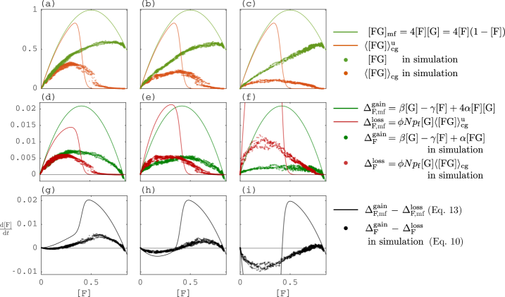
Figure S3: Emergent relations between key quantities and forest area $\raisebox{1.07639pt}{\scalebox{0.8}{[}}\mathrm{F}\raisebox{1.07639pt}{\scalebox{0.8}{]}}$ compared to the mean field with site percolation (dots: simulations, lines: corresponding mean field quantities from Section S4S4.2): (a–c) forest perimeter $\raisebox{1.07639pt}{\scalebox{0.8}{[}}\mathrm{FG}\raisebox{1.07639pt}{\scalebox{0.8}{]}}$ (green) and grassland-weighted forest perimeter $\langle\raisebox{1.07639pt}{\scalebox{0.8}{[}}\mathrm{FG}\raisebox{1.07639pt}{\scalebox{0.8}{]}}\rangle_{\mathrm{cg}}$ (orange), where green line equals $4\raisebox{1.07639pt}{\scalebox{0.8}{[}}\mathrm{F}\raisebox{1.07639pt}{\scalebox{0.8}{]}}\raisebox{1.07639pt}{\scalebox{0.8}{[}}\mathrm{G}\raisebox{1.07639pt}{\scalebox{0.8}{]}}$ and orange line was called $\langle\raisebox{1.07639pt}{\scalebox{0.8}{[}}\mathrm{FG}\raisebox{1.07639pt}{\scalebox{0.8}{]}}\rangle_{\mathrm{cg}}^{u}$ in the main article, (d–f) forest gain terms and loss terms in Eqs. 5 and 6, (g–i) forest area rate of change $(\mathrm{d}/\mathrm{d}t)\raisebox{1.07639pt}{\scalebox{0.8}{[}}\mathrm{F}\raisebox{1.07639pt}{\scalebox{0.8}{]}}$ from Eq. 9. Columns correspond to vertical dashed lines in Fig. 2 ($\phi N{=}0.257,\phi N{=}0.38,\phi N{=}1.32$). Simulation results are identical to Fig. 4. Domain size: $N{=}100\mathrm{x}100$ cells. See Section S4S4.2 for details of derivation for $\langle\raisebox{1.07639pt}{\scalebox{0.8}{[}}\mathrm{FG}\raisebox{1.07639pt}{\scalebox{0.8}{]}}\rangle_{\mathrm{cg}}^{\mathrm{u}}$ and $\raisebox{1.07639pt}{\scalebox{0.8}{[}}\mathrm{FG}\raisebox{1.07639pt}{\scalebox{0.8}{]}}_{\mathrm{mf}}$.

S2 Relevant characteristics of the fire spreading process

Before obtaining the mean-field equations for coupled vegetation and fire dynamics, we analyse the fire spreading process in isolation. The insights from this section will enable us to set up a mean-field model that constitutes the fairest comparison against the analysis in the main text.

S2.1 Definition and mean field

When we remove state $\mathrm{F}$ and its conversion rates to/from other types ($\alpha,\beta,\gamma,\rho_{\mathrm{f}}$) from the FGBA process, the dynamics show fire spread alone. We call this the GBA process. Writing $\mathrm{x}_{i}$ as shorthand for $\delta_{\mathrm{x}}(X_{i})$ (equalling $1$ if $X_{i}=\mathrm{x}$ and $0$ otherwise) and taking expectations in each cell $i$, we obtain equations for the rate of change of the expectation that cell $i$ is occupied by species $x\in\{\mathrm{G},\mathrm{B},\mathrm{A}\}$,

$$\frac{\mathrm{d}}{\mathrm{d}t}\bigl{\langle}\mathrm{G}_{i}\bigr{\rangle} =\lambda\bigl{\langle}\mathrm{A}_{i}\bigr{\rangle}-\bigl{\langle}\mathrm{G}_{i}(\phi+\sum_{j\in{\cal N}(i)}\rho_{\mathrm{g}}\mathrm{B}_{j})\bigr{\rangle},$$

$$\frac{\mathrm{d}}{\mathrm{d}t}\bigl{\langle}\mathrm{B}_{i}\bigr{\rangle} =\phi\bigl{\langle}\mathrm{G}_{i}\bigr{\rangle}-\mu\bigl{\langle}\mathrm{B}_{i}\bigr{\rangle}+\bigl{\langle}\rho_{\mathrm{g}}\mathrm{G}_{i}\sum_{j\in{\cal N}(i)}\mathrm{B}_{j}\bigr{\rangle}, \quad\underset{\frac{1}{N}\sum_{i}^{N}}{\;\;\Longrightarrow}$$

$$\frac{\mathrm{d}}{\mathrm{d}t}\bigl{\langle}\mathrm{A}_{i}\bigr{\rangle} =-\frac{\mathrm{d}}{\mathrm{d}t}\bigl{\langle}\mathrm{G}_{i}\bigr{\rangle}-\frac{\mathrm{d}}{\mathrm{d}t}\bigl{\langle}\mathrm{B}_{i}\bigr{\rangle}=\mu\bigl{\langle}\mathrm{B}_{i}\bigr{\rangle}-\lambda\bigl{\langle}\mathrm{A}_{i}\bigr{\rangle},$$

$$\frac{\mathrm{d}}{\mathrm{d}t}\langle\raisebox{1.07639pt}{\scalebox{0.8}{[}}\mathrm{G}\raisebox{1.07639pt}{\scalebox{0.8}{]}}\rangle =\lambda\langle\raisebox{1.07639pt}{\scalebox{0.8}{[}}\mathrm{A}\raisebox{1.07639pt}{\scalebox{0.8}{]}}\rangle-\phi\langle\raisebox{1.07639pt}{\scalebox{0.8}{[}}\mathrm{G}\raisebox{1.07639pt}{\scalebox{0.8}{]}}\rangle-\rho_{\mathrm{g}}\langle\raisebox{1.07639pt}{\scalebox{0.8}{[}}\mathrm{GB}\raisebox{1.07639pt}{\scalebox{0.8}{]}}\rangle,$$

$$\frac{\mathrm{d}}{\mathrm{d}t}\langle\raisebox{1.07639pt}{\scalebox{0.8}{[}}\mathrm{B}\raisebox{1.07639pt}{\scalebox{0.8}{]}}\rangle =\phi\langle\raisebox{1.07639pt}{\scalebox{0.8}{[}}\mathrm{G}\raisebox{1.07639pt}{\scalebox{0.8}{]}}\rangle-\mu\langle\raisebox{1.07639pt}{\scalebox{0.8}{[}}\mathrm{B}\raisebox{1.07639pt}{\scalebox{0.8}{]}}\rangle+\rho_{\mathrm{g}}\langle\raisebox{1.07639pt}{\scalebox{0.8}{[}}\mathrm{GB}\raisebox{1.07639pt}{\scalebox{0.8}{]}}\rangle,$$ (S1)

$$\frac{\mathrm{d}}{\mathrm{d}t}\langle\raisebox{1.07639pt}{\scalebox{0.8}{[}}\mathrm{A}\raisebox{1.07639pt}{\scalebox{0.8}{]}}\rangle =\mu\langle\raisebox{1.07639pt}{\scalebox{0.8}{[}}\mathrm{B}\raisebox{1.07639pt}{\scalebox{0.8}{]}}\rangle-\lambda\langle\raisebox{1.07639pt}{\scalebox{0.8}{[}}\mathrm{A}\raisebox{1.07639pt}{\scalebox{0.8}{]}}\rangle,$$

where $\langle\cdot\rangle$ are ensemble averages, $\raisebox{1.07639pt}{\scalebox{0.8}{[}}\mathrm{x}\raisebox{1.07639pt}{\scalebox{0.8}{]}}$ the domain fraction of species $\mathrm{x}$, and $\raisebox{1.07639pt}{\scalebox{0.8}{[}}\mathrm{xy}\raisebox{1.07639pt}{\scalebox{0.8}{]}}$ the total number of neighbouring $\mathrm{xy}$ pairs divided by $N$, later referred to as the $\mathrm{xy}$ interface or $\mathrm{xy}$ perimeter. This set of equations can be derived rigorously from the master equation (e.g. Tomé and De Oliveira, 2015). To go from individual (left) to population level (right), we summed over $i$ and divided by $N$, using Eq. M1. Section S2S2.1 is not a closed system. To close the system, we need to determine all undetermined terms $\raisebox{1.07639pt}{\scalebox{0.8}{[}}\mathrm{xy}\raisebox{1.07639pt}{\scalebox{0.8}{]}}$ on the right-hand side without creating new unknowns. The simplest way to do this is to assume absence of pairwise correlations, i.e. $\langle\raisebox{1.07639pt}{\scalebox{0.8}{[}}\mathrm{xy}\raisebox{1.07639pt}{\scalebox{0.8}{]}}\rangle=4\langle\raisebox{1.07639pt}{\scalebox{0.8}{[}}\mathrm{x}\raisebox{1.07639pt}{\scalebox{0.8}{]}}\rangle\langle\raisebox{1.07639pt}{\scalebox{0.8}{[}}\mathrm{y}\raisebox{1.07639pt}{\scalebox{0.8}{]}}\rangle$. We take the additional assumption of $N\to\infty$, such that the law of large numbers applies and $\raisebox{1.07639pt}{\scalebox{0.8}{[}}\mathrm{x}\raisebox{1.07639pt}{\scalebox{0.8}{]}}\to\langle\raisebox{1.07639pt}{\scalebox{0.8}{[}}\mathrm{x}\raisebox{1.07639pt}{\scalebox{0.8}{]}}\rangle$. These assumptions are valid when all cells in an large domain interact with each other at uniform contact rates of order $1/N$. This results in the simple mean-field approximation of the GBA process:

$$\dot{\raisebox{1.07639pt}{\scalebox{0.8}{[}}\mathrm{G}\raisebox{1.07639pt}{\scalebox{0.8}{]}}} =\lambda\raisebox{1.07639pt}{\scalebox{0.8}{[}}\mathrm{A}\raisebox{1.07639pt}{\scalebox{0.8}{]}}-\phi\raisebox{1.07639pt}{\scalebox{0.8}{[}}\mathrm{G}\raisebox{1.07639pt}{\scalebox{0.8}{]}}-4\rho_{\mathrm{g}}\raisebox{1.07639pt}{\scalebox{0.8}{[}}\mathrm{G}\raisebox{1.07639pt}{\scalebox{0.8}{]}}\raisebox{1.07639pt}{\scalebox{0.8}{[}}\mathrm{B}\raisebox{1.07639pt}{\scalebox{0.8}{]}},$$

$$\dot{\raisebox{1.07639pt}{\scalebox{0.8}{[}}\mathrm{B}\raisebox{1.07639pt}{\scalebox{0.8}{]}}} =\phi\raisebox{1.07639pt}{\scalebox{0.8}{[}}\mathrm{G}\raisebox{1.07639pt}{\scalebox{0.8}{]}}-\mu\raisebox{1.07639pt}{\scalebox{0.8}{[}}\mathrm{B}\raisebox{1.07639pt}{\scalebox{0.8}{]}}+4\rho_{\mathrm{g}}\raisebox{1.07639pt}{\scalebox{0.8}{[}}\mathrm{G}\raisebox{1.07639pt}{\scalebox{0.8}{]}}\raisebox{1.07639pt}{\scalebox{0.8}{[}}\mathrm{B}\raisebox{1.07639pt}{\scalebox{0.8}{]}},$$ (S2)

$$\dot{\raisebox{1.07639pt}{\scalebox{0.8}{[}}\mathrm{A}\raisebox{1.07639pt}{\scalebox{0.8}{]}}} =\mu\raisebox{1.07639pt}{\scalebox{0.8}{[}}\mathrm{B}\raisebox{1.07639pt}{\scalebox{0.8}{]}}-\lambda\raisebox{1.07639pt}{\scalebox{0.8}{[}}\mathrm{A}\raisebox{1.07639pt}{\scalebox{0.8}{]}},$$

where we also used the dot notation for time derivatives. Substituting $\raisebox{1.07639pt}{\scalebox{0.8}{[}}\mathrm{A}\raisebox{1.07639pt}{\scalebox{0.8}{]}}=1-\raisebox{1.07639pt}{\scalebox{0.8}{[}}\mathrm{G}\raisebox{1.07639pt}{\scalebox{0.8}{]}}-\raisebox{1.07639pt}{\scalebox{0.8}{[}}\mathrm{B}\raisebox{1.07639pt}{\scalebox{0.8}{]}}$ and taking only the independent equations, we finally obtain

$$\dot{\raisebox{1.07639pt}{\scalebox{0.8}{[}}\mathrm{G}\raisebox{1.07639pt}{\scalebox{0.8}{]}}} =\lambda(1-\raisebox{1.07639pt}{\scalebox{0.8}{[}}\mathrm{G}\raisebox{1.07639pt}{\scalebox{0.8}{]}}-\raisebox{1.07639pt}{\scalebox{0.8}{[}}\mathrm{B}\raisebox{1.07639pt}{\scalebox{0.8}{]}})-\phi\raisebox{1.07639pt}{\scalebox{0.8}{[}}\mathrm{G}\raisebox{1.07639pt}{\scalebox{0.8}{]}}-4\rho_{\mathrm{g}}\raisebox{1.07639pt}{\scalebox{0.8}{[}}\mathrm{G}\raisebox{1.07639pt}{\scalebox{0.8}{]}}\raisebox{1.07639pt}{\scalebox{0.8}{[}}\mathrm{B}\raisebox{1.07639pt}{\scalebox{0.8}{]}},$$ (S3)

$$\dot{\raisebox{1.07639pt}{\scalebox{0.8}{[}}\mathrm{B}\raisebox{1.07639pt}{\scalebox{0.8}{]}}} =\phi\raisebox{1.07639pt}{\scalebox{0.8}{[}}\mathrm{G}\raisebox{1.07639pt}{\scalebox{0.8}{]}}-\mu\raisebox{1.07639pt}{\scalebox{0.8}{[}}\mathrm{B}\raisebox{1.07639pt}{\scalebox{0.8}{]}}+4\rho_{\mathrm{g}}\raisebox{1.07639pt}{\scalebox{0.8}{[}}\mathrm{G}\raisebox{1.07639pt}{\scalebox{0.8}{]}}\raisebox{1.07639pt}{\scalebox{0.8}{[}}\mathrm{B}\raisebox{1.07639pt}{\scalebox{0.8}{]}}.$$

We further focus on the case $\phi=0$, the reason for which will become clear below. When $\phi=0$, Eq. S3 has two steady states, a trivial one at $(\raisebox{1.07639pt}{\scalebox{0.8}{[}}\mathrm{G}\raisebox{1.07639pt}{\scalebox{0.8}{]}},\raisebox{1.07639pt}{\scalebox{0.8}{[}}\mathrm{B}\raisebox{1.07639pt}{\scalebox{0.8}{]}})=(1,0)$ and one at $(\raisebox{1.07639pt}{\scalebox{0.8}{[}}\mathrm{G}\raisebox{1.07639pt}{\scalebox{0.8}{]}},\raisebox{1.07639pt}{\scalebox{0.8}{[}}\mathrm{B}\raisebox{1.07639pt}{\scalebox{0.8}{]}})=(\frac{\mu}{4\rho_{\mathrm{g}}},\frac{1-\mu/4\rho_{g}}{1+\mu/\lambda})$. The eigenvalues of the Jacobian of Eq. S3 show that for $4\rho_{\mathrm{g}}/\mu>1$, the trivial steady states is a saddle and the non-trivial a spiral sink. For $4\rho_{\mathrm{g}}/\mu<1$, the trivial state state is a stable node and the only physical solution. Hence, the steady states exchange stability at the transcritical bifurcation at $4\rho_{\mathrm{g}}/\mu=1$. The GBA process with $\phi=0$ is equivalent to the SIRS spreading process in epidemiology Kiss et al. (2017), which represents spread of a disease in a population with waning immunity. Fire $\mathrm{B}$ plays the role of infected individuals. Infections spread through a population of susceptibles $\mathrm{G}$ at rate $\rho_{\mathrm{g}}$ per $\mathrm{GB}$ link. They subsequently acquire a state of immunity $\mathrm{A}$ at rate $\mu$, which can be lost at rate $\lambda$. The non-trivial steady state corresponds to the endemic equilibrium and the transcritical bifurcation to the epidemic threshold $R_{0}$.

S2.2 Extinction in finite systems

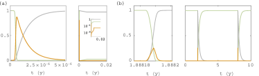
Figure S4: Time series of the GBA process ($\lambda,\phi\neq 0$): (a) mean-field approximation, (b) simulation on a square lattice. G: green, B: orange, A: grey.

A well-known characteristic of this spreading process with $\phi=0$ and $\raisebox{1.07639pt}{\scalebox{0.8}{[}}\mathrm{B}\raisebox{1.07639pt}{\scalebox{0.8}{]}}_{0}>0$ is that in finite systems, it goes extinct in finite time, even when $R_{0}>1$ (Durrett, 1995). This is so because stochastic excursions away from the non-trivial equilibrium will eventually reach the absorbing trivial state. When the spontaneous ignition rate $\phi>0$ and the time to extinction is much smaller than the typical waiting time between ignition events, there are repeated fire events separated by extinction events. The dynamics then effectively behave as a series of GBA processes with $\phi=0$ and $\raisebox{1.07639pt}{\scalebox{0.8}{[}}\mathrm{B}\raisebox{1.07639pt}{\scalebox{0.8}{]}}_{0}>0$. This is what we observe in cellular automaton simulations on a square lattice of $100{\times}100$ cells for realistic parameters (Fig. S4b, right panel). The mean-field approximation (Eq. S3), on the other hand, does not show extinction due to its assumption of $N\to\infty$. Instead, it shows a single pulse (Fig. S4a, left panel) after which a high-ash low-grass and non-zero fire steady state (the endemic equilibrium) is reached (Fig. S4a, right panel). In the case $\phi=0$, the required lattice size to avoid extinction with high probability depends on the initial conditions Durrett (1995), but for realistic parameter ranges, it is unrealistically large. This can be understood as follows.

• When the initial condition is a single fire, at least one cell has to keep on burning until the density of grass has regrown to a level sufficient for a new wave to propagate. This translates into the condition $(L/\Delta x)^{2}\exp(-\mu/\lambda)\geq{\cal O}(1)$, such that $L\geq{\cal O}(10^{4\cdot 10^{4}})$ for our parameters (taking a grid size of $\Delta x=0.03\text{km}$ as in Hébert-Dufresne et al. (2018)).

• When initial conditions are such that a band of the domain is immune at the start, a single fire can keep on burning by crossing the domain repeatedly Durrett (1995). When assuming $\rho_{\mathrm{g}}\gg\mu$ and using that waiting times between spreading events are exponentially distributed with mean $1/\rho_{\mathrm{g}}$, a fire will spread throughout the domain in a time of the order $\tau\approx L/(\rho_{\mathrm{g}}\Delta x)$. For there to be sufficient regrowth of grass on this time scale, we need $L/(\rho_{\mathrm{g}}\Delta x)\approx 1/\lambda$, or $L\approx\rho_{\mathrm{g}}\Delta x/\lambda$. For the parameters we have chosen, this means $L={\cal O}(10^{4})$km, i.e. the order of magnitude of the earth’s circumference, which is drastically smaller than the above estimate yet still impractically large.

Taking more conservative estimates for fire spreading rates or taking account of a small positive fire ignition rate $\phi={\cal O}(\lambda/N)$ for the initial condition with a single burning cell, this may be decreased by an order of magnitude, i.e. the size of a continent or country. Still, in reality, extinction will occur on smaller scales due to spatiotemporal heterogeneity of forcing parameters as a consequence of climatic seasonality or existence of natural or artificial boundaries (such as forests), leading to a lower effective system size. Hence, in any real system, repeated extinction and system-scale oscillations are to be expected.

S2.3 Percolation analysis of a single fire event

Therefore, a single fire in realistically sized systems corresponds to the case $\phi=0$, starting with a single burning cell. Using that the regrowth of grass occurs on a much slower time scale, we can further also set $\lambda=0$ in our following analysis. The GBA process with $\phi,\lambda=0$ is equivalent to susceptible-infected-recovered (SIR) epidemic spreading (Kiss et al., 2017). The final size of the epidemic in SIR epidemic spreading on a lattice shows a continuous phase transition (CPT) at a critical spreading rate $\rho_{\mathrm{g}}$ and scaling laws near the critical point obey those of the ordinary percolation universality class (Tomé and Ziff, 2010). Figure S5 shows mean quantities for SIR epidemic spreading on a square lattice in a range of infection probabilities and initial number of immune individuals, which are spatially uniformly distributed. In particular, we show that SIR epidemic spreading is a type of mixed site-bond percolation, with bond occupation probability given by $p_{b}:=p_{\mathrm{g}}=\rho_{\mathrm{g}}/(\rho_{\mathrm{g}}+\mu)$ (which is fixed at $0.9$ in the main text, as in ref. (Hébert-Dufresne et al., 2018)) and site occupation probability given by $p_{s}:=\raisebox{1.07639pt}{\scalebox{0.8}{[}}\mathrm{G}\raisebox{1.07639pt}{\scalebox{0.8}{]}}_{0}$, i.e. the initial fraction of cells that are grass in fire spreading, or the complement of the initial fraction of immune individuals in epidemic spreading (with the rest being susceptible). In Fig. S5, we record the mean cumulative probability of being burnt $\langle Q\rangle$ and the susceptibility $\chi$ of $\langle Q\rangle$, defined as

$$Q :=\frac{\raisebox{1.07639pt}{\scalebox{0.8}{[}}\mathrm{A}\raisebox{1.07639pt}{\scalebox{0.8}{]}}^{*}-\raisebox{1.07639pt}{\scalebox{0.8}{[}}\mathrm{A}\raisebox{1.07639pt}{\scalebox{0.8}{]}}_{0}}{\raisebox{1.07639pt}{\scalebox{0.8}{[}}\mathrm{G}\raisebox{1.07639pt}{\scalebox{0.8}{]}}_{0}},$$ (S4)

$$\chi =\frac{\langle Q^{2}\rangle}{\langle Q\rangle},$$ (S5)

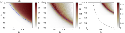
Figure S5: GBA process with $\phi{=}\lambda{=}0$ (equivalent to square lattice SIR spreading): $\langle Q\rangle,\chi$ versus bond occupation probability $p_{b}:=p_{\mathrm{g}}$ (Eq. 3) and site occupation probability $p_{s}{=}\raisebox{1.07639pt}{\scalebox{0.8}{[}}\mathrm{G}\raisebox{1.07639pt}{\scalebox{0.8}{]}}_{0}$. (a) Mean cumulative probability of being burnt $\langle Q\rangle$ (expectation of Eq. S4). (b) Susceptibility $\chi$ (Eq. S5). (c) Susceptibility $\chi$ compared to the mean-field percolation threshold $p_{s,\mathrm{mf}}$, given in Eq. S6 (dashed black). The dash-dotted blue line indicates the location of the infinite-size percolation threshold for uncorrelated mixed site-bond percolation (taken from (Tarasevich and Van Der Marck, 1999)). The GBA model’s percolation threshold lies at higher values (b) due to spatial correlation of $p_{\mathrm{g}}$ as explained in the text. The colour scale was taken from Crameri (2018). See Fig. S11 for more detail.

where $\raisebox{1.07639pt}{\scalebox{0.8}{[}}\mathrm{\cdot}\raisebox{1.07639pt}{\scalebox{0.8}{]}}_{0}$ denotes initial value and $\raisebox{1.07639pt}{\scalebox{0.8}{[}}\mathrm{\cdot}\raisebox{1.07639pt}{\scalebox{0.8}{]}}^{*}$ final value. For $N{\to}\infty$, $\langle Q\rangle$ converges to the percolation probability $P_{\infty}$, which is the probability that a grass cell belongs to the giant connected component. We use the location where $\chi$ peaks as an estimate of the percolation threshold Hébert-Dufresne and Allard (2019); Stauffer and Aharony (1994). When $p_{s}=\raisebox{1.07639pt}{\scalebox{0.8}{[}}\mathrm{G}\raisebox{1.07639pt}{\scalebox{0.8}{]}}_{0}=1$, we have pure bond percolation and when $\rho_{\mathrm{g}}/\mu\to\infty$, we have pure site percolation. The percolation threshold for standard mixed site-bond percolation (from (Tarasevich and Van Der Marck, 1999)) is shown in Fig. S5 with a dot-dashed blue curve. The pure bond percolation threshold (when $\raisebox{1.07639pt}{\scalebox{0.8}{[}}\mathrm{G}\raisebox{1.07639pt}{\scalebox{0.8}{]}}_{0}=1$) of SIR epidemic spreading occurs at higher $p_{b}$ than in standard bond percolation ($p_{b}\approx 0.538>0.5$) because the possibility of spreading to multiple neighbours makes the bond occupation probability spatially autocorrelated, as shown by (Tomé and Ziff, 2010). The pure site percolation limit shows the classical value (for the square lattice) of $\raisebox{1.07639pt}{\scalebox{0.8}{[}}\mathrm{G}\raisebox{1.07639pt}{\scalebox{0.8}{]}}_{0}\approx 0.593$. From Eq. S3 (with $\phi=\lambda=0$), we can obtain the mean-field percolation threshold $p_{s,\mathrm{mf}}$ by finding where the trivial state becomes unstable in Eq. S3, which is given by

$$4\raisebox{1.07639pt}{\scalebox{0.8}{[}}\mathrm{G}\raisebox{1.07639pt}{\scalebox{0.8}{]}}_{0}\frac{\rho_{\mathrm{g}}}{\mu}=1\;\implies\;p_{s,\mathrm{mf}}=\raisebox{1.07639pt}{\scalebox{0.8}{[}}\mathrm{G}\raisebox{1.07639pt}{\scalebox{0.8}{]}}_{0}=\frac{1}{4}\left(\frac{1}{p_{b}}-1\right).$$ (S6)

As shown in Fig. S5c, the mean-field approximation shows a large bias towards lower values.

Implications for the FGBA process

On landscapes with forest, fires can be blocked (albeit imperfectly) by forest cells. These landscapes obtain a steady state shape due to the shaping processes of forest demography and fire. Hence, results from the spatially uniform $\raisebox{1.07639pt}{\scalebox{0.8}{[}}\mathrm{G}\raisebox{1.07639pt}{\scalebox{0.8}{]}}_{0}$ above do not apply to percolation effects in the full FGBA process. That is, when fire spreads on landscapes with forest, the critical point for pure site percolation ($\rho_{\mathrm{g}}/\mu\to\infty$, or $p_{\mathrm{g}}\to 1$) will in general depend not only on the site occupation probability $\raisebox{1.07639pt}{\scalebox{0.8}{[}}\mathrm{G}\raisebox{1.07639pt}{\scalebox{0.8}{]}}_{0}$ but also on the spatial correlation function of site occupation. For the idealised case of fire-proof forest ($p_{\mathrm{f}}=0$), fire percolation on real landscapes is then equivalent to correlated mixed percolation, where correlations in bond occupation probability occur due to the spreading process, and correlations in site occupation probability occur due to the nonrandom spatial structure of the landscape. When $p_{\mathrm{f}}>0$, the spreading process becomes a heterogeneous (correlated) bond percolation processes, i.e. a percolation process in which fire spread on grass occurs with bond occupation probability $p_{\mathrm{g}}$ and on forest with bond occupation probability $p_{\mathrm{f}}$. The possibility of spreading on forest decreases the percolation thresholds compared to the correlated mixed percolation limit of $p_{\mathrm{f}}\to 0$. This decrease is expected to be small because forests do not spread fires well ($p_{\mathrm{f}}\approx 0$).

S3 Simple mean field of joint forest and fire spread

When we follow the same steps as in S2S2.1, we obtain the simple mean-field approximation of the FGBA process:

$$\dot{\raisebox{1.07639pt}{\scalebox{0.8}{[}}\mathrm{G}\raisebox{1.07639pt}{\scalebox{0.8}{]}}} =\lambda\raisebox{1.07639pt}{\scalebox{0.8}{[}}\mathrm{A}\raisebox{1.07639pt}{\scalebox{0.8}{]}}-\phi\raisebox{1.07639pt}{\scalebox{0.8}{[}}\mathrm{G}\raisebox{1.07639pt}{\scalebox{0.8}{]}}-4\rho_{\mathrm{g}}\raisebox{1.07639pt}{\scalebox{0.8}{[}}\mathrm{G}\raisebox{1.07639pt}{\scalebox{0.8}{]}}\raisebox{1.07639pt}{\scalebox{0.8}{[}}\mathrm{B}\raisebox{1.07639pt}{\scalebox{0.8}{]}}-\beta\raisebox{1.07639pt}{\scalebox{0.8}{[}}\mathrm{G}\raisebox{1.07639pt}{\scalebox{0.8}{]}}-4\alpha\raisebox{1.07639pt}{\scalebox{0.8}{[}}\mathrm{F}\raisebox{1.07639pt}{\scalebox{0.8}{]}}\raisebox{1.07639pt}{\scalebox{0.8}{[}}\mathrm{G}\raisebox{1.07639pt}{\scalebox{0.8}{]}}+\gamma\raisebox{1.07639pt}{\scalebox{0.8}{[}}\mathrm{F}\raisebox{1.07639pt}{\scalebox{0.8}{]}},$$

$$\dot{\raisebox{1.07639pt}{\scalebox{0.8}{[}}\mathrm{F}\raisebox{1.07639pt}{\scalebox{0.8}{]}}} =\beta\raisebox{1.07639pt}{\scalebox{0.8}{[}}\mathrm{A}\raisebox{1.07639pt}{\scalebox{0.8}{]}}+4\alpha\raisebox{1.07639pt}{\scalebox{0.8}{[}}\mathrm{F}\raisebox{1.07639pt}{\scalebox{0.8}{]}}\raisebox{1.07639pt}{\scalebox{0.8}{[}}\mathrm{A}\raisebox{1.07639pt}{\scalebox{0.8}{]}}-4\rho_{\mathrm{f}}\raisebox{1.07639pt}{\scalebox{0.8}{[}}\mathrm{F}\raisebox{1.07639pt}{\scalebox{0.8}{]}}\raisebox{1.07639pt}{\scalebox{0.8}{[}}\mathrm{B}\raisebox{1.07639pt}{\scalebox{0.8}{]}}+\beta\raisebox{1.07639pt}{\scalebox{0.8}{[}}\mathrm{G}\raisebox{1.07639pt}{\scalebox{0.8}{]}}+4\alpha\raisebox{1.07639pt}{\scalebox{0.8}{[}}\mathrm{F}\raisebox{1.07639pt}{\scalebox{0.8}{]}}\raisebox{1.07639pt}{\scalebox{0.8}{[}}\mathrm{G}\raisebox{1.07639pt}{\scalebox{0.8}{]}}-\gamma\raisebox{1.07639pt}{\scalebox{0.8}{[}}\mathrm{F}\raisebox{1.07639pt}{\scalebox{0.8}{]}},$$ (S7)

$$\dot{\raisebox{1.07639pt}{\scalebox{0.8}{[}}\mathrm{B}\raisebox{1.07639pt}{\scalebox{0.8}{]}}} =\phi\raisebox{1.07639pt}{\scalebox{0.8}{[}}\mathrm{G}\raisebox{1.07639pt}{\scalebox{0.8}{]}}-\mu\raisebox{1.07639pt}{\scalebox{0.8}{[}}\mathrm{B}\raisebox{1.07639pt}{\scalebox{0.8}{]}}+4\rho_{\mathrm{f}}\raisebox{1.07639pt}{\scalebox{0.8}{[}}\mathrm{F}\raisebox{1.07639pt}{\scalebox{0.8}{]}}\raisebox{1.07639pt}{\scalebox{0.8}{[}}\mathrm{B}\raisebox{1.07639pt}{\scalebox{0.8}{]}}+4\rho_{\mathrm{g}}\raisebox{1.07639pt}{\scalebox{0.8}{[}}\mathrm{G}\raisebox{1.07639pt}{\scalebox{0.8}{]}}\raisebox{1.07639pt}{\scalebox{0.8}{[}}\mathrm{B}\raisebox{1.07639pt}{\scalebox{0.8}{]}},$$

$$\dot{\raisebox{1.07639pt}{\scalebox{0.8}{[}}\mathrm{A}\raisebox{1.07639pt}{\scalebox{0.8}{]}}} =\mu\raisebox{1.07639pt}{\scalebox{0.8}{[}}\mathrm{B}\raisebox{1.07639pt}{\scalebox{0.8}{]}}-\lambda\raisebox{1.07639pt}{\scalebox{0.8}{[}}\mathrm{A}\raisebox{1.07639pt}{\scalebox{0.8}{]}}-\beta\raisebox{1.07639pt}{\scalebox{0.8}{[}}\mathrm{A}\raisebox{1.07639pt}{\scalebox{0.8}{]}}-4\alpha\raisebox{1.07639pt}{\scalebox{0.8}{[}}\mathrm{F}\raisebox{1.07639pt}{\scalebox{0.8}{]}}\raisebox{1.07639pt}{\scalebox{0.8}{[}}\mathrm{A}\raisebox{1.07639pt}{\scalebox{0.8}{]}}.$$

The simple mean field shows bistability of tree cover (first shown by ref. (Hébert-Dufresne et al., 2018) for $\gamma=0$) in ranges of all parameters that are expected to show considerable spatial heterogeneity in a given ecosystem: $\alpha,\beta,\gamma,\phi$ (Fig. S6). However, despite being qualitatively correct, it shows a large bias compared to simulations. For the parameter ranges of our simulations, it has no non-trivial solution for positive fire ignition rate $\phi$, so we had to choose different parameter values to find its bistability range. This bias is due to the inability of the simple mean to capture two effects: repeated fire extinction on a fast timescale and the spatial nature of the two spreading processes. In the following section, we derive alternative mean-field models that partially correct for these biases.

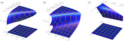
Figure S6: Steady states and bifurcations of forest cover $\raisebox{1.07639pt}{\scalebox{0.8}{[}}\mathrm{F}\raisebox{1.07639pt}{\scalebox{0.8}{]}}$ in the simple mean field of the FGBA process (blue: steady state manifold, green/orange contours at fixed axis values, red: saddle-node bifurcations): (a) versus fire ignition rate $\phi$ and forest spreading rate $\alpha$, (b) versus fire ignition rate $\phi$ and spontaneous forest growth rate $\beta$, (c) versus fire ignition rate $\phi$ and spontaneous forest mortality rate $\gamma$. Due to its large bias, the simple mean field shows different bistability ranges than the simulations. We set $p_{\mathrm{g}}{=}0.25$ (requiring a $\rho_{\mathrm{g}}$ that is 27x smaller than in simulations) such that bistability ranges are visible (remaining parameters are as in Table M1).

S4 Two-timescale mean field of joint forest and fire spread

Here, we derive an alternative mean-field model that takes account of separation of fire events in systems with realistic sizes, assuming that fire spread occurs on a much faster time scale than forest spread. This means that we can consider the fire spreading process in isolation with $\phi=\lambda=0$ (as argued in Section S2), and take the asymptotic amount of forest burnt by a single fire before extinction on the fast time scale as forest mortality per fire event on the slow time scale.

S4.1 Well-mixed fire and forest

We start with the simplest case, where both vegetation and fire mix uniformly, which is one way to conform with the mean-field assumption of absence of correlations.

S4.1.1 Fast process: forest loss due to a single fire

On the fast time scale, we can set all small parameters related to forest demography, grass regrowth and fire ignition to zero ($\alpha{=}\beta{=}\gamma{=}\lambda{=}\phi{=}0$), such that we obtain

$$\frac{\mathrm{d}}{\mathrm{d}t}\raisebox{1.07639pt}{\scalebox{0.8}{[}}\mathrm{G}\raisebox{1.07639pt}{\scalebox{0.8}{]}} =-4\rho_{\mathrm{g}}\raisebox{1.07639pt}{\scalebox{0.8}{[}}\mathrm{G}\raisebox{1.07639pt}{\scalebox{0.8}{]}}\raisebox{1.07639pt}{\scalebox{0.8}{[}}\mathrm{B}\raisebox{1.07639pt}{\scalebox{0.8}{]}},$$

$$\frac{\mathrm{d}}{\mathrm{d}t}\raisebox{1.07639pt}{\scalebox{0.8}{[}}\mathrm{F}\raisebox{1.07639pt}{\scalebox{0.8}{]}} =-4\rho_{\mathrm{f}}\raisebox{1.07639pt}{\scalebox{0.8}{[}}\mathrm{F}\raisebox{1.07639pt}{\scalebox{0.8}{]}}\raisebox{1.07639pt}{\scalebox{0.8}{[}}\mathrm{B}\raisebox{1.07639pt}{\scalebox{0.8}{]}},$$ (S8)

$$\frac{\mathrm{d}}{\mathrm{d}t}\raisebox{1.07639pt}{\scalebox{0.8}{[}}\mathrm{B}\raisebox{1.07639pt}{\scalebox{0.8}{]}} =-\mu\raisebox{1.07639pt}{\scalebox{0.8}{[}}\mathrm{B}\raisebox{1.07639pt}{\scalebox{0.8}{]}}+4\rho_{\mathrm{f}}\raisebox{1.07639pt}{\scalebox{0.8}{[}}\mathrm{F}\raisebox{1.07639pt}{\scalebox{0.8}{]}}\raisebox{1.07639pt}{\scalebox{0.8}{[}}\mathrm{B}\raisebox{1.07639pt}{\scalebox{0.8}{]}}+4\rho_{\mathrm{g}}\raisebox{1.07639pt}{\scalebox{0.8}{[}}\mathrm{G}\raisebox{1.07639pt}{\scalebox{0.8}{]}}\raisebox{1.07639pt}{\scalebox{0.8}{[}}\mathrm{B}\raisebox{1.07639pt}{\scalebox{0.8}{]}},$$

$$\frac{\mathrm{d}}{\mathrm{d}t}\raisebox{1.07639pt}{\scalebox{0.8}{[}}\mathrm{A}\raisebox{1.07639pt}{\scalebox{0.8}{]}} =\mu\raisebox{1.07639pt}{\scalebox{0.8}{[}}\mathrm{B}\raisebox{1.07639pt}{\scalebox{0.8}{]}},$$

where the products arise from the well-mixedness assumption as before. By rewriting the equations for $\frac{\mathrm{d}}{\mathrm{d}t}\raisebox{1.07639pt}{\scalebox{0.8}{[}}\mathrm{G}\raisebox{1.07639pt}{\scalebox{0.8}{]}},\frac{\mathrm{d}}{\mathrm{d}t}\raisebox{1.07639pt}{\scalebox{0.8}{[}}\mathrm{F}\raisebox{1.07639pt}{\scalebox{0.8}{]}},\frac{\mathrm{d}}{\mathrm{d}t}\raisebox{1.07639pt}{\scalebox{0.8}{[}}\mathrm{A}\raisebox{1.07639pt}{\scalebox{0.8}{]}}$ as

$$-\frac{1}{4\rho_{\mathrm{g}}\raisebox{1.07639pt}{\scalebox{0.8}{[}}\mathrm{G}\raisebox{1.07639pt}{\scalebox{0.8}{]}}}\frac{\mathrm{d}}{\mathrm{d}t}\raisebox{1.07639pt}{\scalebox{0.8}{[}}\mathrm{G}\raisebox{1.07639pt}{\scalebox{0.8}{]}} =-\frac{1}{4\rho_{\mathrm{f}}\raisebox{1.07639pt}{\scalebox{0.8}{[}}\mathrm{F}\raisebox{1.07639pt}{\scalebox{0.8}{]}}}\frac{\mathrm{d}}{\mathrm{d}t}\raisebox{1.07639pt}{\scalebox{0.8}{[}}\mathrm{F}\raisebox{1.07639pt}{\scalebox{0.8}{]}}=\frac{1}{\mu}\frac{\mathrm{d}}{\mathrm{d}t}\raisebox{1.07639pt}{\scalebox{0.8}{[}}\mathrm{A}\raisebox{1.07639pt}{\scalebox{0.8}{]}}=\raisebox{1.07639pt}{\scalebox{0.8}{[}}\mathrm{B}\raisebox{1.07639pt}{\scalebox{0.8}{]}},$$ (S9)

we can obtain $\raisebox{1.07639pt}{\scalebox{0.8}{[}}\mathrm{G}\raisebox{1.07639pt}{\scalebox{0.8}{]}}$ and $\raisebox{1.07639pt}{\scalebox{0.8}{[}}\mathrm{F}\raisebox{1.07639pt}{\scalebox{0.8}{]}}$ as a function of $\raisebox{1.07639pt}{\scalebox{0.8}{[}}\mathrm{A}\raisebox{1.07639pt}{\scalebox{0.8}{]}}$ via separation of variables and integration:

$$\raisebox{1.07639pt}{\scalebox{0.8}{[}}\mathrm{G}\raisebox{1.07639pt}{\scalebox{0.8}{]}}(t)=\raisebox{1.07639pt}{\scalebox{0.8}{[}}\mathrm{G}\raisebox{1.07639pt}{\scalebox{0.8}{]}}_{0}\exp\bigl{(}-\frac{4\rho_{\mathrm{g}}}{\mu}\raisebox{1.07639pt}{\scalebox{0.8}{[}}\mathrm{A}\raisebox{1.07639pt}{\scalebox{0.8}{]}}(t)\bigr{)},\quad \raisebox{1.07639pt}{\scalebox{0.8}{[}}\mathrm{F}\raisebox{1.07639pt}{\scalebox{0.8}{]}}(t)=\raisebox{1.07639pt}{\scalebox{0.8}{[}}\mathrm{F}\raisebox{1.07639pt}{\scalebox{0.8}{]}}_{0}\exp\bigl{(}-\frac{4\rho_{\mathrm{f}}}{\mu}\raisebox{1.07639pt}{\scalebox{0.8}{[}}\mathrm{A}\raisebox{1.07639pt}{\scalebox{0.8}{]}}(t)\bigr{)}.$$ (S10)

Substituting Eq. S10 into the equation for $\frac{\mathrm{d}}{\mathrm{d}t}\raisebox{1.07639pt}{\scalebox{0.8}{[}}\mathrm{A}\raisebox{1.07639pt}{\scalebox{0.8}{]}}$ in Section S4S4.1S4.1.1 and setting the time derivative to zero, we obtain an implicit relation of the asymptotic amount of vegetation burnt:

$$\raisebox{1.07639pt}{\scalebox{0.8}{[}}\mathrm{A}\raisebox{1.07639pt}{\scalebox{0.8}{]}}^{*} =1-\raisebox{1.07639pt}{\scalebox{0.8}{[}}\mathrm{G}\raisebox{1.07639pt}{\scalebox{0.8}{]}}^{*}-\raisebox{1.07639pt}{\scalebox{0.8}{[}}\mathrm{F}\raisebox{1.07639pt}{\scalebox{0.8}{]}}^{*}=1-\raisebox{1.07639pt}{\scalebox{0.8}{[}}\mathrm{G}\raisebox{1.07639pt}{\scalebox{0.8}{]}}_{0}\exp\bigl{(}-\frac{4\rho_{\mathrm{g}}}{\mu}\raisebox{1.07639pt}{\scalebox{0.8}{[}}\mathrm{A}\raisebox{1.07639pt}{\scalebox{0.8}{]}}^{*}\bigr{)}-\raisebox{1.07639pt}{\scalebox{0.8}{[}}\mathrm{F}\raisebox{1.07639pt}{\scalebox{0.8}{]}}_{0}\exp\bigl{(}-\frac{4\rho_{\mathrm{f}}}{\mu}\raisebox{1.07639pt}{\scalebox{0.8}{[}}\mathrm{A}\raisebox{1.07639pt}{\scalebox{0.8}{]}}^{*}\bigr{)}.$$ (S11)

When taking an initial state consisting of only grass and forest, that is $\raisebox{1.07639pt}{\scalebox{0.8}{[}}\mathrm{G}\raisebox{1.07639pt}{\scalebox{0.8}{]}}_{0}=1-\raisebox{1.07639pt}{\scalebox{0.8}{[}}\mathrm{F}\raisebox{1.07639pt}{\scalebox{0.8}{]}}_{0}$, $\raisebox{1.07639pt}{\scalebox{0.8}{[}}\mathrm{A}\raisebox{1.07639pt}{\scalebox{0.8}{]}}^{*}$ can be found numerically as a function of $\rho_{\mathrm{g}}/\mu,\rho_{\mathrm{f}}/\mu$ and $\raisebox{1.07639pt}{\scalebox{0.8}{[}}\mathrm{F}\raisebox{1.07639pt}{\scalebox{0.8}{]}}_{0}$. This can in turn be used to obtain the total amount of forest lost due to a single fire, from Eq. S10,

$$\Delta\raisebox{1.07639pt}{\scalebox{0.8}{[}}\mathrm{F}\raisebox{1.07639pt}{\scalebox{0.8}{]}}_{\mathrm{mf}}:=\raisebox{1.07639pt}{\scalebox{0.8}{[}}\mathrm{F}\raisebox{1.07639pt}{\scalebox{0.8}{]}}_{0}-\raisebox{1.07639pt}{\scalebox{0.8}{[}}\mathrm{F}\raisebox{1.07639pt}{\scalebox{0.8}{]}}^{*}=\raisebox{1.07639pt}{\scalebox{0.8}{[}}\mathrm{F}\raisebox{1.07639pt}{\scalebox{0.8}{]}}_{0}\Bigl{(}1-\exp\bigl{(}-\frac{4\rho_{\mathrm{g}}}{\mu}\raisebox{1.07639pt}{\scalebox{0.8}{[}}\mathrm{A}\raisebox{1.07639pt}{\scalebox{0.8}{]}}^{*}\bigr{)}\Bigr{)},$$ (S12)

where subscript $\mathrm{mf}$ denotes mean field. A plot of Equation S12 versus $\raisebox{1.07639pt}{\scalebox{0.8}{[}}\mathrm{F}\raisebox{1.07639pt}{\scalebox{0.8}{]}}$ is given in Fig. S7 (solid purple curve), which shows that the percolation threshold – where forest starts blocking fire – lies at unrealistically low grass cover, as was also the case for perfectly blocking forest (Fig. S5c, dashed line).

S4.1.2 Slow processes: forest demography and fire damage

Now, we can define the mean-field forest gain and loss terms on the slow time scale as

$$\Delta_{\mathrm{F},\mathrm{mf}}^{\mathrm{gain}} :=\beta\raisebox{1.07639pt}{\scalebox{0.8}{[}}\mathrm{G}\raisebox{1.07639pt}{\scalebox{0.8}{]}}+4\alpha\raisebox{1.07639pt}{\scalebox{0.8}{[}}\mathrm{F}\raisebox{1.07639pt}{\scalebox{0.8}{]}}\raisebox{1.07639pt}{\scalebox{0.8}{[}}\mathrm{G}\raisebox{1.07639pt}{\scalebox{0.8}{]}}-\gamma\raisebox{1.07639pt}{\scalebox{0.8}{[}}\mathrm{F}\raisebox{1.07639pt}{\scalebox{0.8}{]}},$$ (S13)

$$\Delta_{\mathrm{F},\mathrm{mf}}^{\mathrm{loss}} :=\phi N\raisebox{1.07639pt}{\scalebox{0.8}{[}}\mathrm{G}\raisebox{1.07639pt}{\scalebox{0.8}{]}}\Delta\raisebox{1.07639pt}{\scalebox{0.8}{[}}\mathrm{F}\raisebox{1.07639pt}{\scalebox{0.8}{]}}_{\mathrm{mf}},$$ (S14)

such that the final mean-field model becomes

$$\frac{\mathrm{d}}{\mathrm{d}t}\raisebox{1.07639pt}{\scalebox{0.8}{[}}\mathrm{F}\raisebox{1.07639pt}{\scalebox{0.8}{]}} =\Delta_{\mathrm{F},\mathrm{mf}}^{\mathrm{gain}}-\Delta_{\mathrm{F},\mathrm{mf}}^{\mathrm{loss}}$$

$$=\beta\raisebox{1.07639pt}{\scalebox{0.8}{[}}\mathrm{G}\raisebox{1.07639pt}{\scalebox{0.8}{]}}+4\alpha\raisebox{1.07639pt}{\scalebox{0.8}{[}}\mathrm{F}\raisebox{1.07639pt}{\scalebox{0.8}{]}}\raisebox{1.07639pt}{\scalebox{0.8}{[}}\mathrm{G}\raisebox{1.07639pt}{\scalebox{0.8}{]}}-\gamma\raisebox{1.07639pt}{\scalebox{0.8}{[}}\mathrm{F}\raisebox{1.07639pt}{\scalebox{0.8}{]}}-\phi N\raisebox{1.07639pt}{\scalebox{0.8}{[}}\mathrm{G}\raisebox{1.07639pt}{\scalebox{0.8}{]}}\Delta\raisebox{1.07639pt}{\scalebox{0.8}{[}}\mathrm{F}\raisebox{1.07639pt}{\scalebox{0.8}{]}}_{\mathrm{mf}},$$

$$=\beta(1-\raisebox{1.07639pt}{\scalebox{0.8}{[}}\mathrm{F}\raisebox{1.07639pt}{\scalebox{0.8}{]}})+4\alpha\raisebox{1.07639pt}{\scalebox{0.8}{[}}\mathrm{F}\raisebox{1.07639pt}{\scalebox{0.8}{]}}(1-\raisebox{1.07639pt}{\scalebox{0.8}{[}}\mathrm{F}\raisebox{1.07639pt}{\scalebox{0.8}{]}})-\gamma\raisebox{1.07639pt}{\scalebox{0.8}{[}}\mathrm{F}\raisebox{1.07639pt}{\scalebox{0.8}{]}}-\phi N(1-\raisebox{1.07639pt}{\scalebox{0.8}{[}}\mathrm{F}\raisebox{1.07639pt}{\scalebox{0.8}{]}})\raisebox{1.07639pt}{\scalebox{0.8}{[}}\mathrm{F}\raisebox{1.07639pt}{\scalebox{0.8}{]}}\Bigl{(}1-\exp\bigl{(}-\frac{4\rho_{\mathrm{g}}}{\mu}\raisebox{1.07639pt}{\scalebox{0.8}{[}}\mathrm{A}\raisebox{1.07639pt}{\scalebox{0.8}{]}}^{*}(\raisebox{1.07639pt}{\scalebox{0.8}{[}}\mathrm{F}\raisebox{1.07639pt}{\scalebox{0.8}{]}})\bigr{)}\Bigr{)}.$$ (S15)

The steady states are shown in Fig. S9 in solid purple for the same parameters as those used in the simulations of the main text. For low and high tree cover, it reproduces the steady states fairly accurately, but unlike the simulations, it shows no wide saddle in between. Hence, while this is an improvement compared to the simple mean field, there is still a large bias at intermediate tree cover. To address this bias, we need drop the assumption of uniform mixing for fire spread.

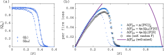
Figure S7: Grass burning probabilities and forest loss per fire in landscapes without spatial structure: (a) probability that a grass cell burns $\langle Q_{p_{\mathrm{g}}}\rangle$, for $p_{\mathrm{g}}=1$ (‘$+$’) and for $p_{\mathrm{g}}=0.9$ (‘$\cdot$’), together with fits to logistic functions; (b) loss per fire estimated from grassland-weighted forest (‘$\times$’, Eq. S16), from $\langle Q_{0.9}\rangle$ (‘$\times$’, Eq. S20), from $\langle Q_{1}\rangle$ (‘$+$’, Eq. S20), by assuming uniform mixing (purple curve, Eq. S12), and measured in fire simulations with uniform random placement of forest (‘$\circ$’).

S4.2 Spatial fire percolation and uniformly randomly placed forest

While the uniform mixing assumption may be ecologically justified for forest spread in case of species with long-range seed dispersal, it is much harder to justify for fire spread, which is fundamentally a local contagion process. Therefore, we aim to take into account the effects of fire as a percolation process while still assuming absence of spatial correlations between forest cells. Because the percolation process affects forest loss, this only affects the loss function. Earlier mean-field models Staver and Levin (2012); Schertzer et al. (2014); Patterson et al. (2021) accounted for the effects of fire percolation by making fire-affected rates threshold functions of tree cover, such as those shown in Fig. S7a, while assuming that vegetation remains spatially uncorrelated (for derivation, see Schertzer et al., 2014). Therefore the mean-field analyses presented here provide the fairest points of comparison.

To estimate the loss due to fire, we will show two alternative approaches. The first is equivalent to our approach in the main text, using grassland-weighted forest perimeter to estimate exposed forest. The second estimates exposed forest via standard results from percolation theory, which are valid here due to the assumption of uniform random placement of forest.

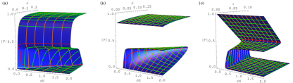
Figure S8: Steady states and bifurcations of forest cover $\raisebox{1.07639pt}{\scalebox{0.8}{[}}\mathrm{F}\raisebox{1.07639pt}{\scalebox{0.8}{]}}$ in the two-timescale mean field of the FGBA process via Item 1 (blue: steady state manifold, green/orange contours at fixed axis values, red: saddle-node bifurcations) as a function of (scaled) fire ignition rate $\phi N$ and: (a) forest spreading rate $\alpha$, (b) spontaneous forest growth rate $\beta$, (c) spontaneous forest mortality rate $\gamma$. Parameters others than the ones on the axes are the same as those chosen in simulations – see Table M1.

1. Using the grassland-weighted forest perimeter $\langle\raisebox{1.07639pt}{\scalebox{0.8}{[}}\mathrm{FG}\raisebox{1.07639pt}{\scalebox{0.8}{]}}\rangle_{\mathrm{cg}}$ (see Eq. 7). According to this approach, fires spread perfectly to the forest perimeter, where a fraction of the forest is burnt. The difference with the main text is that the landscapes in which fire spreads have uniform random placement of forest. We indicate this difference below by the superscript $\mathrm{u}$ in $\langle\raisebox{1.07639pt}{\scalebox{0.8}{[}}\mathrm{FG}\raisebox{1.07639pt}{\scalebox{0.8}{]}}\rangle_{\mathrm{cg}}^{\mathrm{u}}$. The resulting loss per fire is

   $$\Delta\raisebox{1.07639pt}{\scalebox{0.8}{[}}\mathrm{F}\raisebox{1.07639pt}{\scalebox{0.8}{]}}_{\mathrm{pu}}=p_{\mathrm{f}}\langle\raisebox{1.07639pt}{\scalebox{0.8}{[}}\mathrm{FG}\raisebox{1.07639pt}{\scalebox{0.8}{]}}\rangle_{\mathrm{cg}}^{\mathrm{u}},$$ (S16)

   such that the loss function is

   $$\Delta_{\mathrm{F},\mathrm{pu}}^{\mathrm{loss}}=\phi N\raisebox{1.07639pt}{\scalebox{0.8}{[}}\mathrm{G}\raisebox{1.07639pt}{\scalebox{0.8}{]}}\Delta\raisebox{1.07639pt}{\scalebox{0.8}{[}}\mathrm{F}\raisebox{1.07639pt}{\scalebox{0.8}{]}}_{\mathrm{pu}}=\phi Np_{\mathrm{f}}\raisebox{1.07639pt}{\scalebox{0.8}{[}}\mathrm{G}\raisebox{1.07639pt}{\scalebox{0.8}{]}}\langle\raisebox{1.07639pt}{\scalebox{0.8}{[}}\mathrm{FG}\raisebox{1.07639pt}{\scalebox{0.8}{]}}\rangle_{\mathrm{cg}}^{\mathrm{u}},$$ (S17)

   where subscript $\mathrm{pu}$ refers to percolation on a square lattice with uniform random placement of forest. The final mean-field model is

   $$\frac{\mathrm{d}}{\mathrm{d}t}\raisebox{1.07639pt}{\scalebox{0.8}{[}}\mathrm{F}\raisebox{1.07639pt}{\scalebox{0.8}{]}} =\Delta_{\mathrm{F},\mathrm{mf}}^{\mathrm{gain}}-\Delta_{\mathrm{F},\mathrm{pu}}^{\mathrm{loss}},$$

   $$=\beta(1-\raisebox{1.07639pt}{\scalebox{0.8}{[}}\mathrm{F}\raisebox{1.07639pt}{\scalebox{0.8}{]}})+4\alpha\raisebox{1.07639pt}{\scalebox{0.8}{[}}\mathrm{F}\raisebox{1.07639pt}{\scalebox{0.8}{]}}(1-\raisebox{1.07639pt}{\scalebox{0.8}{[}}\mathrm{F}\raisebox{1.07639pt}{\scalebox{0.8}{]}})-\gamma\raisebox{1.07639pt}{\scalebox{0.8}{[}}\mathrm{F}\raisebox{1.07639pt}{\scalebox{0.8}{]}}-\phi Np_{\mathrm{f}}(1-\raisebox{1.07639pt}{\scalebox{0.8}{[}}\mathrm{F}\raisebox{1.07639pt}{\scalebox{0.8}{]}})\langle\raisebox{1.07639pt}{\scalebox{0.8}{[}}\mathrm{FG}\raisebox{1.07639pt}{\scalebox{0.8}{]}}\rangle_{\mathrm{cg}}^{\mathrm{u}}(\raisebox{1.07639pt}{\scalebox{0.8}{[}}\mathrm{F}\raisebox{1.07639pt}{\scalebox{0.8}{]}}),$$ (S18)

   where we made explicit that $\langle\raisebox{1.07639pt}{\scalebox{0.8}{[}}\mathrm{FG}\raisebox{1.07639pt}{\scalebox{0.8}{]}}\rangle_{\mathrm{cg}}^{\mathrm{u}}$ is a function of $\raisebox{1.07639pt}{\scalebox{0.8}{[}}\mathrm{F}\raisebox{1.07639pt}{\scalebox{0.8}{]}}$. This mean-field model shows clear bistability for the same parameter ranges as in simulations (Fig. S8). For the exact same parameters, this mean-field is qualitatively most comparable to simulations, but the saddle is much flatter (Fig. S9, solid blue line versus black dots).

2. Using percolation theory. Alternatively, we can estimate forest loss using mean burning probabilities from percolation due to a single fire. The forest perimeter exposed to fire for a given realisation is the interface of burnt grass with forest at the end of the fire $\raisebox{1.07639pt}{\scalebox{0.8}{[}}\mathrm{FA}\raisebox{1.07639pt}{\scalebox{0.8}{]}}^{*}$. When we take the expectation (for given total grass cover) and forest cells are assumed to be uniformly randomly placed, we have

   $$\langle\raisebox{1.07639pt}{\scalebox{0.8}{[}}\mathrm{FA}\raisebox{1.07639pt}{\scalebox{0.8}{]}}^{*}\rangle=\langle 4\raisebox{1.07639pt}{\scalebox{0.8}{[}}\mathrm{F}\raisebox{1.07639pt}{\scalebox{0.8}{]}}\raisebox{1.07639pt}{\scalebox{0.8}{[}}\mathrm{A}\raisebox{1.07639pt}{\scalebox{0.8}{]}}^{*}\rangle=4\raisebox{1.07639pt}{\scalebox{0.8}{[}}\mathrm{F}\raisebox{1.07639pt}{\scalebox{0.8}{]}}\raisebox{1.07639pt}{\scalebox{0.8}{[}}\mathrm{G}\raisebox{1.07639pt}{\scalebox{0.8}{]}}\langle Q_{p_{\mathrm{g}}}\rangle,$$ (S19)

   where $\langle Q_{p_{\mathrm{g}}}\rangle$ is the mean proportion of grass that burns for given $p_{\mathrm{g}}$ and $\raisebox{1.07639pt}{\scalebox{0.8}{[}}\mathrm{G}\raisebox{1.07639pt}{\scalebox{0.8}{]}}$ (see Eq. S4; shown in Fig. S5b). The loss per fire in this case is then

   $$\Delta\raisebox{1.07639pt}{\scalebox{0.8}{[}}\mathrm{F}\raisebox{1.07639pt}{\scalebox{0.8}{]}}_{\mathrm{pu}}=4p_{\mathrm{f}}\raisebox{1.07639pt}{\scalebox{0.8}{[}}\mathrm{F}\raisebox{1.07639pt}{\scalebox{0.8}{]}}\raisebox{1.07639pt}{\scalebox{0.8}{[}}\mathrm{G}\raisebox{1.07639pt}{\scalebox{0.8}{]}}\langle Q_{p_{\mathrm{g}}}\rangle,$$ (S20)

   such that the loss function is (multiplying by $\phi N\raisebox{1.07639pt}{\scalebox{0.8}{[}}\mathrm{G}\raisebox{1.07639pt}{\scalebox{0.8}{]}}$)

   $$\Delta_{\mathrm{F},\mathrm{pu}}^{\mathrm{loss}}=4p_{\mathrm{f}}\phi N\raisebox{1.07639pt}{\scalebox{0.8}{[}}\mathrm{G}\raisebox{1.07639pt}{\scalebox{0.8}{]}}^{2}\raisebox{1.07639pt}{\scalebox{0.8}{[}}\mathrm{F}\raisebox{1.07639pt}{\scalebox{0.8}{]}}\langle Q_{p_{\mathrm{g}}}\rangle.$$ (S21)

   The final mean-field model is then

   $$\frac{\mathrm{d}}{\mathrm{d}t}\raisebox{1.07639pt}{\scalebox{0.8}{[}}\mathrm{F}\raisebox{1.07639pt}{\scalebox{0.8}{]}} =\beta(1-\raisebox{1.07639pt}{\scalebox{0.8}{[}}\mathrm{F}\raisebox{1.07639pt}{\scalebox{0.8}{]}})+4\alpha\raisebox{1.07639pt}{\scalebox{0.8}{[}}\mathrm{F}\raisebox{1.07639pt}{\scalebox{0.8}{]}}(1-\raisebox{1.07639pt}{\scalebox{0.8}{[}}\mathrm{F}\raisebox{1.07639pt}{\scalebox{0.8}{]}})-\gamma\raisebox{1.07639pt}{\scalebox{0.8}{[}}\mathrm{F}\raisebox{1.07639pt}{\scalebox{0.8}{]}}-4p_{\mathrm{f}}\phi N(1-\raisebox{1.07639pt}{\scalebox{0.8}{[}}\mathrm{F}\raisebox{1.07639pt}{\scalebox{0.8}{]}})^{2}\raisebox{1.07639pt}{\scalebox{0.8}{[}}\mathrm{F}\raisebox{1.07639pt}{\scalebox{0.8}{]}}\langle Q_{p_{\mathrm{g}}}\rangle.$$ (S22)

   This mean-field model has very similar steady states as Item 1 but the saddle is slightly lower (dotted blue line in Fig. S9). In the limit of large domain size, $\langle Q_{p_{\mathrm{g}}}\rangle$ may be replaced by the percolation probability $P_{\infty}$, which is defined as the probability that a grass cell belongs to the giant component Christensen and Moloney (2005) (see also Fig. S11a).

Both of the estimates above assume that $p_{\mathrm{f}}=0$ for fire spread and that $p_{\mathrm{f}}$ is small for loss of (uniformly randomly placed) forest due to fire. The first further assumes that fire spreads perfectly on grass ($p_{\mathrm{g}}=1$). Therefore the two estimates are equivalent when the spreading process is pure site percolation, for which $\langle\raisebox{1.07639pt}{\scalebox{0.8}{[}}\mathrm{FG}\raisebox{1.07639pt}{\scalebox{0.8}{]}}\rangle_{\mathrm{cg}}=4\langle Q_{1}\rangle\raisebox{1.07639pt}{\scalebox{0.8}{[}}\mathrm{F}\raisebox{1.07639pt}{\scalebox{0.8}{]}}\raisebox{1.07639pt}{\scalebox{0.8}{[}}\mathrm{G}\raisebox{1.07639pt}{\scalebox{0.8}{]}}$ (equating Eq. S17 and Eq. S21), which is confirmed by Fig. S7b (‘$\times$’ and ‘$+$’ symbols). Comparing the estimates to recorded forest loss in fire simulations where only the assumption of random placement is taken (‘$\circ$’ in Fig. S7b), one sees that the second estimate (‘$\cdot$’ in Fig. S7b) is more accurate than the first estimate (‘$\times$’ in Fig. S7b), despite that it carries more assumptions. Hence, the error due to the assumption of grass perfectly spreading compensates the error by the assumption of forest perfectly blocking fire. We expect that the difference between the two approaches will be smaller for landscapes with spatial aggregation of forest, where fires spread in pockets of high grass cover, for which $\langle Q_{1}\rangle-\langle Q_{0.9}\rangle$ is smaller (Fig. S7a).

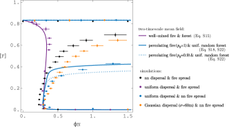
Figure S9: Comparison of steady state forest as a function of ignition rate in the time-separated mean-field and in simulations (dots with error bars: simulations, lines: mean field). See legend for details. Note, ‘uniform random’ refers to the placement of forest cells in the domain.

S4.3 Detailed comparison against simulations

Here, we compare the time-separated mean-field models to the simulations of the main text and also to other simulations with different spreading ranges for forest and/or fire. In Fig. S9, dots with error bars are simulations and lines are mean-field approximations. The black dots are the simulations from the main text, with nearest-neighbour spreading for both fire and forest. Purple dots are simulations where both fire and forest can spread to any other cell. Blue dots are simulations where forest can spread to any other cell, but fire spreads along nearest neighbours. And finally, orange dots denote simulations where forest spread occurs in a Gaussian neighbourhood with standard deviation 60m (two cells).

All simulations and approximations agree fairly well on the parameter value where the lower saddle-node bifurcation occurs. All except the fully well-mixed case agree on the stable steady states. The disagreement occurs particularly for the unstable steady states, where the effect of spatial structure is hence most pronounced and process-dependent. There is little or no bistability in the well-mixed two-timescale mean-field (purple line) but its good agreement with uniformly mixed simulations (purple dots) further indicates the validity of the assumption of time-scale separation with well-separated fire events. The mean field where fire is a site percolation process on landscapes with uniform random placement of forest (blue line), is qualitatively more correct but it has a much flatter saddle than the simulations (black dots). Hence, even the mean-field model that takes into account the effects of percolation while keeping forest cells spatially uncorrelated remains strongly biased due to the importance of spatial aggregation of forest cells. Taking larger neighbourhood sizes in the simulations does not change this (orange dots). Even compared to simulations with uniform forest dispersal (blue dots), the mean field with site percolation shows some bias, indicating that the fire spreading alone already induces some spatial structure. This is most likely caused by lower survival rates of solitary compared to aggregated forest cells.

The bias of the mean field is even more apparent in the dynamics. Figure S3 shows the same figure as Fig. 4, but with the corresponding values of the mean field with site percolation on top. Panels a–c show large differences between $\raisebox{1.07639pt}{\scalebox{0.8}{[}}\mathrm{FG}\raisebox{1.07639pt}{\scalebox{0.8}{]}}$ and $\langle\raisebox{1.07639pt}{\scalebox{0.8}{[}}\mathrm{FG}\raisebox{1.07639pt}{\scalebox{0.8}{]}}\rangle_{\mathrm{cg}}$ of simulations (scattered dots) versus those from the mean field (curves). In particular, while for the mean field, the perimeter is the parabola $\raisebox{1.07639pt}{\scalebox{0.8}{[}}\mathrm{FG}\raisebox{1.07639pt}{\scalebox{0.8}{]}}=4\raisebox{1.07639pt}{\scalebox{0.8}{[}}\mathrm{F}\raisebox{1.07639pt}{\scalebox{0.8}{]}}\raisebox{1.07639pt}{\scalebox{0.8}{[}}\mathrm{G}\raisebox{1.07639pt}{\scalebox{0.8}{]}}=4\raisebox{1.07639pt}{\scalebox{0.8}{[}}\mathrm{F}\raisebox{1.07639pt}{\scalebox{0.8}{]}}(1-\raisebox{1.07639pt}{\scalebox{0.8}{[}}\mathrm{F}\raisebox{1.07639pt}{\scalebox{0.8}{]}})$, the perimeter of simulations lies below this parabola for any $\raisebox{1.07639pt}{\scalebox{0.8}{[}}\mathrm{F}\raisebox{1.07639pt}{\scalebox{0.8}{]}}$. That the simulated perimeter is lower for given forest area means that forest is more spatially aggregated in simulations. This results in lower forest growth rate at any cover value (panels d–f) because fewer forest cells can expand into grass. Fire-induced damage is lower below $\raisebox{1.07639pt}{\scalebox{0.8}{[}}\mathrm{F}\raisebox{1.07639pt}{\scalebox{0.8}{]}}\approx 0.4$ and higher above (panels d–f). This is so because damage per fire (at given cover) is determined by two effects: exposure of forest and clustering of grass. Below $\raisebox{1.07639pt}{\scalebox{0.8}{[}}\mathrm{F}\raisebox{1.07639pt}{\scalebox{0.8}{]}}\approx 0.4$, there is no clustering, such that only decreased exposure due to aggregation can decrease forest loss. Above $\raisebox{1.07639pt}{\scalebox{0.8}{[}}\mathrm{F}\raisebox{1.07639pt}{\scalebox{0.8}{]}}\approx 0.4$, aggregation decreases clustering, such that grassland stays fully connected at higher forest cover than in the case with uniform random placement, with larger fires as a consequence. This further leads to an upward shift of the unstable forest state compared to the mean field (panels (g–i), see also Fig. S9). The effect of forest aggregation on fire spread has an equivalent in disease spread: in the SIR process, aggregation of immune individuals lowers the epidemic threshold, such that it elevates the population immunisation threshold to eradicate the epidemic Keeling (1999). Note though, that, as argued above, the equivalent epidemic process to tropical fire spread in forest-grassland landscapes is not the regular SIR process, but one that has a mix of two populations: susceptibles (grass) and imperfectly immunised individuals (forest).

S5 Evolution of fronts — heterogeneous states

Here, we illustrate the case where grass and forest are initially separated into two contiguous areas with their interface extending along a straight line. Because for this type of initial conditions, the single-cluster approximation (Eq. 11) is valid, we can focus on the evolution of the interface. As spontaneous conversion between forest and grass (with rates $\beta$ and $\gamma$) increases independence between cells and promotes homogeneity at large scale, we expect the effects of heterogeneous initial conditions to be most persistent when the spontaneous conversion rates $\beta$ and $\gamma$ are small. Therefore, we will set $\beta=\gamma=0$, for which Eq. 9 becomes

$$\frac{\mathrm{d}\raisebox{1.07639pt}{\scalebox{0.8}{[}}\mathrm{F}\raisebox{1.07639pt}{\scalebox{0.8}{]}}}{\mathrm{d}t}=(\alpha-\phi p_{\mathrm{f}}N\raisebox{1.07639pt}{\scalebox{0.8}{[}}\mathrm{G}\raisebox{1.07639pt}{\scalebox{0.8}{]}})\raisebox{1.07639pt}{\scalebox{0.8}{[}}\mathrm{FG}\raisebox{1.07639pt}{\scalebox{0.8}{]}}.$$ (S23)

Hence, the precise shape of the interface $\raisebox{1.07639pt}{\scalebox{0.8}{[}}\mathrm{FG}\raisebox{1.07639pt}{\scalebox{0.8}{]}}$ does not affect the location of the steady states, only the rate at which they are approached or receded from. The trivial steady states of Eq. S23 are $\raisebox{1.07639pt}{\scalebox{0.8}{[}}\mathrm{F}\raisebox{1.07639pt}{\scalebox{0.8}{]}}=0$ and $\raisebox{1.07639pt}{\scalebox{0.8}{[}}\mathrm{F}\raisebox{1.07639pt}{\scalebox{0.8}{]}}=1$ (where $\raisebox{1.07639pt}{\scalebox{0.8}{[}}\mathrm{FG}\raisebox{1.07639pt}{\scalebox{0.8}{]}}=0$), which are stable, and between them, there is the saddle

$$\raisebox{1.07639pt}{\scalebox{0.8}{[}}\mathrm{F}\raisebox{1.07639pt}{\scalebox{0.8}{]}}^{*}=1-\frac{\alpha}{\phi Np_{\mathrm{f}}}.$$ (S24)

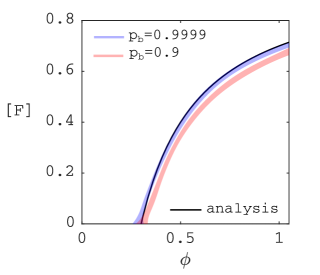
Figure S12: Saddle of Eq. S23 via Eq. S24 (single cluster – solid black) compared to controlled simulations (shaded red: $p_{\mathrm{g}}=\rho_{\mathrm{g}}/(\rho_{\mathrm{g}}+\mu)=0.9$, shaded blue: $p_{\mathrm{g}}=0.9999$) in case of heterogeneous initial conditions and without spontaneous interactions ($\beta{=}\gamma{=}0$). Other parameters: $\alpha{=}0.03,\rho_{\mathrm{f}}{=}1.11\cdot 10^{5},\mu{=}10^{6},\lambda{=}5$.

As seen in Fig. S12, this analytical prediction (solid black) matches the controlled simulations with $p_{\mathrm{g}}=0.9999$ (shaded blue). For $p_{\mathrm{g}}=0.9$ (shaded red), which we used before, there is a small bias. In the limit of $N\to\infty$, Eq. S24 converges to $\raisebox{1.07639pt}{\scalebox{0.8}{[}}\mathrm{F}\raisebox{1.07639pt}{\scalebox{0.8}{]}}^{*}_{\infty}=1$, implying that in an infinite domain, any positive fire rate leads to extinction of forest below $\raisebox{1.07639pt}{\scalebox{0.8}{[}}\mathrm{F}\raisebox{1.07639pt}{\scalebox{0.8}{]}}^{*}=1$. When ignoring the effect of ash, this would also occur for heterogeneous initial conditions. That is, considering an infinite domain with many grass clusters of which the size is a random variable (with support $[0,\infty)$), there will be initial grass clusters of arbitrarily large size, which will expand and eventually drive forest extinct. However, such determinism does not occur in the simulations because at high fire rates, patches with ash start to block fires, and the rate of exposure of the forest interface to fire becomes limited by the rate at which ash is converted back into grass. As a first correction for this, one can multiply $p_{\mathrm{f}}$ with the average proportion of grass sites that are in the ash state after the expected waiting time between fires $1-\exp(-\lambda/\phi N)$, such that $\raisebox{1.07639pt}{\scalebox{0.8}{[}}\mathrm{F}\raisebox{1.07639pt}{\scalebox{0.8}{]}}^{*}_{\infty}=1-\alpha/\lambda p_{\mathrm{f}}$. Keeping in mind that we are focusing on heterogeneous states, the analysis here implies that for $\gamma=\beta=0$, there is a critical patch size above which the forest patch expands and below which it contracts. The intuition is that above the critical forest patch size, there is not enough grass area to reach the minimum number of ignitions required to erode the forest.

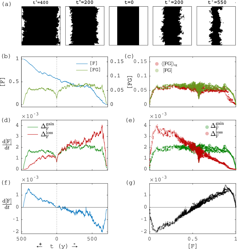
Figure S10: Perimeter quantities and change rates according to Eq. 9 when initial conditions are heterogeneous and there are no spontaneous transitions ($\beta{=}\gamma{=}0$) for $\phi{=}6.98\cdot 10^{-5}$, displayed as in Figs. 3 and 4. (a) Snapshots of the domain at indicated times. (b,d,f) Cover, interface and rate of change from Eq. 9 versus time. (c,e,g) Interface, grass-cluster weighted average of the interface, and rate of change from Eq. 9 versus cover. Remaining parameters are $\alpha{=}0.03,\rho_{\mathrm{g}}{=}10^{10},\rho_{\mathrm{f}}{=}1.11\cdot 10^{5},\mu{=}10^{6},\lambda{=}5$.

In Fig. S10, we show how the dynamics and steady states arise from $\raisebox{1.07639pt}{\scalebox{0.8}{[}}\mathrm{FG}\raisebox{1.07639pt}{\scalebox{0.8}{]}}$, as we did in Fig. 3 and Fig. 4, but now starting with separated patches of grass and forest that interface on a line on both sides (showing for $\raisebox{1.07639pt}{\scalebox{0.8}{[}}\mathrm{F}\raisebox{1.07639pt}{\scalebox{0.8}{]}}_{0}=0.57$). From $\raisebox{1.07639pt}{\scalebox{0.8}{[}}\mathrm{FG}\raisebox{1.07639pt}{\scalebox{0.8}{]}}(0)=2L/N=2N^{-1/2}=0.02$, the interface quickly gains roughness due to the dynamics, until it reaches a steady state of $\raisebox{1.07639pt}{\scalebox{0.8}{[}}\mathrm{FG}\raisebox{1.07639pt}{\scalebox{0.8}{]}}^{*}\approx 6L/N=6N^{-1/2}=0.06$ (see Fig. S10a–c). Figure S10b confirms that $\langle\raisebox{1.07639pt}{\scalebox{0.8}{[}}\mathrm{FG}\raisebox{1.07639pt}{\scalebox{0.8}{]}}\rangle_{\mathrm{cg}}\approx\raisebox{1.07639pt}{\scalebox{0.8}{[}}\mathrm{FG}\raisebox{1.07639pt}{\scalebox{0.8}{]}}$ (except when forest cover approaches $\raisebox{1.07639pt}{\scalebox{0.8}{[}}\mathrm{F}\raisebox{1.07639pt}{\scalebox{0.8}{]}}=0$ or $\raisebox{1.07639pt}{\scalebox{0.8}{[}}\mathrm{F}\raisebox{1.07639pt}{\scalebox{0.8}{]}}=1$), confirming that the single-cluster approximation is valid. Away from $\raisebox{1.07639pt}{\scalebox{0.8}{[}}\mathrm{F}\raisebox{1.07639pt}{\scalebox{0.8}{]}}=0$ and $\raisebox{1.07639pt}{\scalebox{0.8}{[}}\mathrm{F}\raisebox{1.07639pt}{\scalebox{0.8}{]}}=1$, $\raisebox{1.07639pt}{\scalebox{0.8}{[}}\mathrm{FG}\raisebox{1.07639pt}{\scalebox{0.8}{]}}$ stays about constant as the forest interface moves (Fig. S10b–c). Therefore the gain and loss terms (as defined in Eqs. 5 and 8) are now, respectively, constant and linearly decreasing with $\raisebox{1.07639pt}{\scalebox{0.8}{[}}\mathrm{F}\raisebox{1.07639pt}{\scalebox{0.8}{]}}$ (Fig. S10e), such that $\mathrm{d}\raisebox{1.07639pt}{\scalebox{0.8}{[}}\mathrm{F}\raisebox{1.07639pt}{\scalebox{0.8}{]}}/\mathrm{d}t$ increases linearly with $\raisebox{1.07639pt}{\scalebox{0.8}{[}}\mathrm{F}\raisebox{1.07639pt}{\scalebox{0.8}{]}}$ (Fig. S10g), except near $\raisebox{1.07639pt}{\scalebox{0.8}{[}}\mathrm{F}\raisebox{1.07639pt}{\scalebox{0.8}{]}}=0$ and $\raisebox{1.07639pt}{\scalebox{0.8}{[}}\mathrm{F}\raisebox{1.07639pt}{\scalebox{0.8}{]}}=1$, where it connects to 0, as here $\raisebox{1.07639pt}{\scalebox{0.8}{[}}\mathrm{FG}\raisebox{1.07639pt}{\scalebox{0.8}{]}}=0$.

S6 A note on finite sizes and bistability

In simple bistable chemical systems, it is known that bistability converges to an abrupt phase transition in the thermodynamic limit ($N{\to}\infty$) Ge and Qian (2009); Thiele et al. (2019), at a value known as the Maxwell point (e.g. Goldenfeld, 2018), making the macroscopic state of the system deterministically dependent on the parameters (e.g. pressure or temperature). With only forest and grass or provided that savanna and forest components are sufficiently decoupled, the same behaviour occurs in spatial mean-field models of tropical forest, with a front between forest and nonforest that is depends deterministically on environmental drivers Wuyts et al. (2019). We do not expect such determinism as $N{\to}\infty$ to arise in the FGBA cellular automaton. The infinite FGBA cellular automaton possesses grass clusters of arbitrary size, such that, even when assuming that fire spreads instantly on grass, there will always be some parts of the forest perimeter shielded from intruding fires by adjacent ash cells. Were it not for this shielding effect, then there would be a deterministic dependence of the dynamics on fire ignition rate away from the absorbing states: $\phi{=}0$ would lead to forest spread while $\phi{>}0$ would lead to forest extinction (see Section S5, for $\beta{=}\gamma{=}0$). In reality, finite fire spreading rates and, in particular, the effects of heterogeneity in space or time impose stronger limits on the reach of fires.

In finite domains, both the cellular automaton and scalar reaction-diffusion equations (with bistable reaction term) show bistability due to critical patch sizes or domain shapes, and dependence on interfacial characteristics (e.g. Liehr, 2013; Goel et al., 2020; Levin, 1979), but this correspondence requires further scrutiny. In realistic scenarios, we then suspect that the amount of bistability depends (besides the parameters) on the ratio of the characteristic interaction scale and the scale of observation. The range of interaction in turn depends on e.g. fire spreading and/or plant dispersal ranges. E.g., if we take as interaction scale the typical size of a savanna fire (assuming that it exists) ${\cal O}(10^{1\ldots 2}\mathrm{km^{2}})$ Andela et al. (2019), this corresponds to an area in the cellular automaton of $100{\times}100$ to $300{\times}300$ cells. This also corresponds to our observation scale (domain size) in the main text. Hence, it may be that the bistability observed in our work is a finite-size effect, and that a larger observation scale leads to more gradual transitions due to existence of multiple stable patterns Rietkerk et al. (2021); Bastiaansen et al. (2022).

S7 How to include fire parameters in existing mean-field models

Previously derived mean-field models of tropical tree cover bistability did not include parameters that relate to fire. Here we give suggestions on how to include fire ignition rate and the appropriate percolation quantities, focusing on the Staver-Levin mean-field model Schertzer et al. (2014); Staver and Levin (2012) of tropical savanna and/or forest bistability. We assume the reader is familiar with Schertzer et al. (2014); Staver and Levin (2012).

By running an infection process on clusters obtained by standard site percolation, Schertzer et al. (2014) used a mixed site-uncorrelated bond-correlated percolation process for fire (although not using this terminology). The site percolation is due to uniformly randomly distributed tree cells perfectly blocking fires and the bond percolation due to flammable cells (grass and savanna saplings in Schertzer et al. (2014)) spreading fires with a given probability. The correlation in bond occupation probability occurs due to the infection dynamics, as explained in Section S2S2.3. One can use the complement of the burning probability of this mixed percolation process, i.e. $1-\langle Q_{p_{\mathrm{b}}}(p_{s})\rangle$, as survival probability instead of that used in Schertzer et al. (2014) (see Fig. S11b for a plot of $\langle Q_{p_{\mathrm{b}}}(p_{s})\rangle$ as a function of the infection probability between flammable cells $p_{b}$ and the probability of a cell being flammable $p_{s}$). If one does so, one can write the mean-field recruitment rate of savanna saplings during a small time interval as $\omega(p_{b},p_{s})\raisebox{1.07639pt}{\scalebox{0.8}{[}}\mathrm{S}\raisebox{1.07639pt}{\scalebox{0.8}{]}}$, where $\omega$ is

$$\omega(p_{b},p_{s}):=\max[\omega_{0}-\phi Np_{s}\langle Q_{p_{\mathrm{b}}}(p_{s})\rangle\Delta\omega,0],$$ (S25)

with $\Delta\omega{>}0$ the per fire decrease in recruitment rate due to burning and $\phi$ the fire ignition rate in flammable cells. Note that, according to Schertzer et al. (2014), the total flammable area is $p_{s}=\raisebox{1.07639pt}{\scalebox{0.8}{[}}\mathrm{S}\raisebox{1.07639pt}{\scalebox{0.8}{]}}+\raisebox{1.07639pt}{\scalebox{0.8}{[}}\mathrm{G}\raisebox{1.07639pt}{\scalebox{0.8}{]}}$ (i.e., the area of grass and savanna saplings). The reasoning is that there are on average $\phi Np_{s}$ ignitions, each causing a fire that on average affects a proportion $\langle Q_{p_{\mathrm{b}}}(p_{s})\rangle$ of flammable cells, thereby lowering the recruitment rate by an amount $\Delta\omega$. If $\raisebox{1.07639pt}{\scalebox{0.8}{[}}\mathrm{S}\raisebox{1.07639pt}{\scalebox{0.8}{]}}$ and $\raisebox{1.07639pt}{\scalebox{0.8}{[}}\mathrm{T}\raisebox{1.07639pt}{\scalebox{0.8}{]}}$ cells are uniformly randomly placed in the area affected by fire, then it follows that the recruitment rate is $\omega(p_{b},p_{s})\raisebox{1.07639pt}{\scalebox{0.8}{[}}\mathrm{S}\raisebox{1.07639pt}{\scalebox{0.8}{]}}$.

For the approximate effect on forest trees (as included in Staver and Levin, 2012), one needs to take into account that forest trees are assumed (in Staver and Levin, 2012) to block fires perfectly. Therefore, they are not in the flammable part of the landscape, but instead share an interface with it. The mean-field rate of forest loss due to fire during a small time interval is then $\zeta(p_{b},p_{s})\raisebox{1.07639pt}{\scalebox{0.8}{[}}\mathrm{F}\raisebox{1.07639pt}{\scalebox{0.8}{]}}$, where $\zeta$ is

$$\zeta(p_{b},p_{s}):=4\phi Np_{s}^{2}p_{\mathrm{f}}\langle Q_{p_{\mathrm{b}}}(p_{s})\rangle,$$ (S26)

with $p_{s}=\raisebox{1.07639pt}{\scalebox{0.8}{[}}\mathrm{S}\raisebox{1.07639pt}{\scalebox{0.8}{]}}+\raisebox{1.07639pt}{\scalebox{0.8}{[}}\mathrm{G}\raisebox{1.07639pt}{\scalebox{0.8}{]}}$ also. The reasoning here is as follows. There are on average $\phi Np_{s}$ ignitions, each causing a fire that affects a proportion $\langle Q_{p_{\mathrm{b}}}(p_{s})\rangle$ of the landscape. Assuming that occurrences of burnt and forest cells are uncorrelated, one can write the interface between them as the number of forest-burnt pairs in a lattice: $4(\langle Q_{p_{\mathrm{b}}}(p_{s})\rangle p_{s})\raisebox{1.07639pt}{\scalebox{0.8}{[}}\mathrm{F}\raisebox{1.07639pt}{\scalebox{0.8}{]}}$. For each such pair, there is a probability $p_{\mathrm{f}}$ of spreading into forest, such that (when using the approximation of small $p_{\mathrm{f}}$ as in the main text), the resulting forest loss is $4\phi Np_{s}^{2}p_{\mathrm{f}}\langle Q_{p_{\mathrm{b}}}(p_{s})\rangle\raisebox{1.07639pt}{\scalebox{0.8}{[}}\mathrm{F}\raisebox{1.07639pt}{\scalebox{0.8}{]}}$.

For large domains, one may replace $\langle Q_{p_{\mathrm{b}}}(p_{s})\rangle$ by the percolation probability $P_{\infty}(p_{b},p_{s})$ (shown in Fig. S11a), which is the probability that a flammable cell is part of the giant connected component.

S8 Additional figures

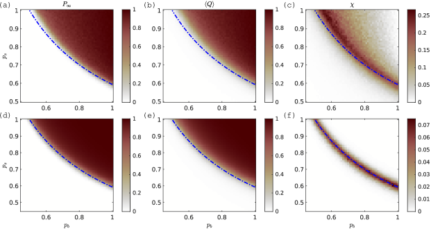
Figure S11: GBA process with $\phi{=}\lambda{=}0$ (equivalent to SIR spreading on the square lattice) in terms of bond occupation probability $p_{b}:=p_{\mathrm{g}}$ (Eq. 3) and site occupation probability $p_{s}:=\raisebox{1.07639pt}{\scalebox{0.8}{[}}\mathrm{G}\raisebox{1.07639pt}{\scalebox{0.8}{]}}_{0}$ (a-c) and compared to standard mixed site-bond percolation (d-f). Shown quantities as a function of bond and site occupation probability (based on 1024 realisations for (a-c) and on 512 realisations for (d-f)): (a,d) percolation probability $P_{\infty}$, (b,e) mean proportion of burnt grass cells $\langle Q\rangle$ (see Eq. S4), and, (c,f) susceptibility $\chi{=}\langle Q^{2}\rangle/\langle Q\rangle$. Percolation probability is defined as the probability that any grass cell belongs to the giant component (Christensen and Moloney, 2005). Susceptibility is defined here as in Hébert-Dufresne and Allard (2019), using $Q$ as order parameter. The dash-dotted blue line indicates the location of the infinite-size percolation threshold for uncorrelated mixed site-bond percolation (taken from (Tarasevich and Van Der Marck, 1999)). For a domain size of 100x100 cells and at the shown resolution, the percolation threshold of mixed site-bond percolation matches that of the infinite size system (f). The GBA process’ percolation threshold lies at higher values (c) due to spatial correlation of $p_{\mathrm{g}}$ as explained in the text. The top row is more noisy than the bottom row because for standard mixed percolation, we were able to obtain the whole distribution of cluster sizes for a each realisation and computed their statistics using percolation theory (Christensen and Moloney, 2005), whereas for the GBA process, each simulation only resulted in one sample. The colour scale was taken from Crameri (2018).

References

- Staver et al. (2011) A. C. Staver, S. Archibald, and S. A. Levin, Science 334, 230 (2011).
- Hirota et al. (2011) M. Hirota, M. Holmgren, E. H. Van Nes, and M. Scheffer, Science 334, 232 (2011).
- de L. Dantas et al. (2016) V. de L. Dantas, M. Hirota, R. S. Oliveira, and J. G. Pausas, Ecology Letters 19, 12 (2016).
- Aleman et al. (2020) J. C. Aleman, A. Fayolle, C. Favier, A. C. Staver, K. G. Dexter, C. M. Ryan, A. F. Azihou, D. Bauman, M. te Beest, E. N. Chidumayo, J. A. Comiskey, J. P. Cromsigt, H. Dessard, J. L. Doucet, M. Finckh, J. F. Gillet, S. Gourlet-Fleury, G. P. Hempson, R. M. Holdo, B. Kirunda, F. N. Kouame, G. Mahy, F. Maiato, P. Gonçalves, I. McNicol, P. N. Quintano, A. J. Plumptre, R. C. Pritchard, R. Revermann, C. B. Schmitt, A. M. Swemmer, H. Talila, E. Woollen, and M. D. Swaine, Proceedings of the National Academy of Sciences of the United States of America 117, 28183 (2020).
- Bond (2008) W. J. Bond, Annual Review of Ecology, Evolution, and Systematics 39, 641 (2008).
- Hoffmann et al. (2012) W. A. Hoffmann, E. L. Geiger, S. G. Gotsch, D. R. Rossatto, L. C. Silva, O. L. Lau, M. Haridasan, and A. C. Franco, Ecology Letters 15, 759 (2012).
- Archibald et al. (2009) S. Archibald, D. P. Roy, B. W. van Wilgen, and R. J. Scholes, Global Change Biology 15, 613 (2009).
- Wuyts et al. (2017) B. Wuyts, A. R. Champneys, and J. I. House, Nature Communications 8, 15519 (2017).
- Van Nes et al. (2018) E. H. Van Nes, A. Staal, S. Hantson, M. Holmgren, S. Pueyo, R. E. Bernardi, B. M. Flores, C. Xu, and M. Scheffer, PloS One 13, e0191027 (2018).
- Schertzer et al. (2014) E. Schertzer, A. C. Staver, and S. A. Levin, Journal of Mathematical Biology 70, 329 (2014).
- Cardoso et al. (2022) A. W. Cardoso, S. Archibald, W. J. Bond, C. Coetsee, M. Forrest, N. Govender, D. Lehmann, L. Makaga, N. Mpanza, J. E. Ndong, A. F. Koumba Pambo, T. Strydom, D. Tilman, P. D. Wragg, and A. C. Staver, Proceedings of the National Academy of Sciences of the United States of America 119 (2022), 10.1073/pnas.2110364119.
- Staver and Levin (2012) A. C. Staver and S. A. Levin, The American Naturalist 180, 211 (2012).
- Lenton et al. (2008) T. M. Lenton, H. Held, E. Kriegler, J. W. Hall, W. Lucht, S. Rahmstorf, and H. J. Schellnhuber, Proceedings of the National Academy of Sciences 105, 1786 (2008).
- Scheffer et al. (2015) M. Scheffer, S. R. Carpenter, V. Dakos, and E. H. Van Nes, Annual Review of Ecology, Evolution, and Systematics 46, 145 (2015).
- Patterson et al. (2021) D. D. Patterson, S. A. Levin, C. Staver, and J. D. Touboul, SIAM Journal on Applied Dynamical Systems 19, 2682 (2021).
- Hébert-Dufresne et al. (2018) L. Hébert-Dufresne, A. F. Pellegrini, U. Bhat, S. Redner, S. W. Pacala, and A. M. Berdahl, Ecology Letters 21, 794 (2018).
- Touboul et al. (2018) J. D. Touboul, A. C. Staver, and S. A. Levin, Proceedings of the National Academy of Sciences , 201712356 (2018).
- Wuyts et al. (2019) B. Wuyts, A. R. Champneys, N. Verschueren, and J. I. House, PLoS ONE 14, e0218151 (2019).
- Goel et al. (2020) N. Goel, V. Guttal, S. A. Levin, and A. C. Staver, American Naturalist 195, 833 (2020).
- Staal et al. (2018) A. Staal, E. H. van Nes, S. Hantson, M. Holmgren, S. C. Dekker, S. Pueyo, C. Xu, and M. Scheffer, Global Change Biology 24, 5096 (2018).
- Li et al. (2019) Q. Li, A. C. Staver, E. Weinan, and S. A. Levin, Theoretical Ecology 12, 237 (2019).
- Dieckmann et al. (2000) U. Dieckmann, R. Law, and J. A. J. Metz, The geometry of ecological interactions : simplifying spatial complexity (Cambridge University Press, 2000) p. 564.
- Wuyts and Sieber (2022) B. Wuyts and J. Sieber, Physical Review E 106, 054312 (2022), arXiv:2111.07643 .
- Keeling (1999) M. J. Keeling, Proceedings of the Royal Society B: Biological Sciences 266, 859 (1999).
- Stauffer and Aharony (1994) D. Stauffer and A. Aharony, Introduction to percolation theory (CRC press, 1994).
- Christensen and Moloney (2005) K. Christensen and N. R. Moloney, Complexity and Criticality, Imperial College Press Advanced Physics Texts, Vol. 1 (Imperial College Press and Distributed, 2005).
- Patterson et al. (2023) D. Patterson, A. C. Staver, S. A. Levin, and J. Touboul, SIAM journal on applied mathematics (2023).
- Bastiaansen et al. (2022) R. Bastiaansen, H. A. Dijkstra, and A. S. V. D. Heydt, Environmental Research Letters 17, 045006 (2022).
- Favier et al. (2004) C. Favier, J. Chave, A. Fabing, D. Schwartz, and M. A. Dubois, Ecological Modelling 171, 85 (2004).
- Aleman and Staver (2018) J. C. Aleman and A. C. Staver, Global Ecology and Biogeography 27, 792 (2018).
- Scheffer et al. (2009) M. Scheffer, J. Bascompte, W. A. Brock, V. Brovkin, S. R. Carpenter, V. Dakos, H. Held, E. H. van Nes, M. Rietkerk, and G. Sugihara, Nature 461, 53 (2009), arXiv:arXiv:1011.1669v3 .
- Boulton et al. (2022) C. A. Boulton, T. M. Lenton, and N. Boers, Nature Climate Change 12, 271 (2022).
- Van Langevelde et al. (2003) F. Van Langevelde, C. A. Van De Vijver, L. Kumar, J. Van De Koppel, N. De Ridder, J. Van Andel, A. K. Skidmore, J. W. Hearne, L. Stroosnijder, W. J. Bond, H. H. Prins, and M. Rietkerk, Ecology 84, 337 (2003).
- Accatino et al. (2010) F. Accatino, C. De Michele, R. Vezzoli, D. Donzelli, and R. J. Scholes, Journal of Theoretical Biology 267, 235 (2010).
- D’Odorico et al. (2006) P. D’Odorico, F. Laio, and L. Ridolfi, The American naturalist 167 (2006), 10.1086/500617.
- Baudena et al. (2010) M. Baudena, F. D’Andrea, and A. Provenzale, Journal of Ecology 98, 74 (2010).
- Beckage et al. (2011) B. Beckage, L. J. Gross, and W. J. Platt, Ecological Modelling 222, 2227 (2011).
- Hoyer-Leitzel and Iams (2021) A. Hoyer-Leitzel and S. Iams, Bulletin of Mathematical Biology 83 (2021), 10.1007/s11538-021-00944-x.
- Spracklen et al. (2018) D. V. Spracklen, J. C. Baker, L. Garcia-Carreras, and J. H. Marsham, “The effects of tropical vegetation on rainfall,” (2018).
- Rietkerk et al. (2021) M. Rietkerk, R. Bastiaansen, S. Banerjee, J. van de Koppel, M. Baudena, and A. Doelman, Science 374 (2021).
- Kiss et al. (2017) I. Z. Kiss, J. C. Miller, and P. L. Simon, Interdisciplinary Applied Mathematics, Interdisciplinary Applied Mathematics, Vol. 46 (Springer International Publishing, Cham, 2017) pp. 1–413.
- Gillespie (2007) D. T. Gillespie, Annual Review of Physical Chemistry 58, 35 (2007).
- Sieber et al. (2008) J. Sieber, A. Gonzalez-Buelga, S. A. Neild, D. J. Wagg, and B. Krauskopf, Phys. Rev. Lett. 100, 244101 (2008).
- Schilder et al. (2015) F. Schilder, E. Bureau, I. F. Santos, J. J. Thomsen, and J. Starke, Journal of Sound and Vibration 358, 251 (2015).
- Barton (2017) D. Barton, Mechanical Systems and Signal Processing 84, 54 (2017).
- Neville et al. (2018) R. M. Neville, R. M. Groh, A. Pirrera, and M. Schenk, Physical review letters 120, 254101 (2018).
- Barton and Sieber (2013) D. A. W. Barton and J. Sieber, Phys. Rev. E 87, 052916 (2013).
- Sieber et al. (2014) J. Sieber, O. E. Omel’chenko, and M. Wolfrum, Phys. Rev. Lett. 112, 054102 (2014).
- Renson et al. (2017) L. Renson, D. Barton, and S. Neild, International Journal of Bifurcation and Chaos 27, 1730002 (2017).
- Kreiss and Lahiri (2012) J. P. Kreiss and S. N. Lahiri, in Handbook of Statistics, Vol. 30 (2012) pp. 3–26.
- Tomé and De Oliveira (2015) T. Tomé and M. J. De Oliveira, Stochastic dynamics and irreversibility (Springer, 2015) p. 394.
- Durrett (1995) R. Durrett, in Epidemic models : their structure and relation to data (New York, NY, 1995) pp. 187–201.
- Tomé and Ziff (2010) T. Tomé and R. M. Ziff, Physical Review E - Statistical, Nonlinear, and Soft Matter Physics 82, 051921 (2010).
- Tarasevich and Van Der Marck (1999) Y. Y. Tarasevich and S. C. Van Der Marck, International Journal of Modern Physics C 10, 1193 (1999).
- Crameri (2018) F. Crameri, “Scientific colour maps,” (2018), http://doi.org/10.5281/zenodo.1243862.
- Hébert-Dufresne and Allard (2019) L. Hébert-Dufresne and A. Allard, Physical Review Research 1, 13009 (2019), arXiv:1810.00735 .
- Ge and Qian (2009) H. Ge and H. Qian, Physical Review Letters 103, 148103 (2009).
- Thiele et al. (2019) U. Thiele, T. Frohoff-Hülsmann, S. Engelnkemper, E. Knobloch, and A. J. Archer, New Journal of Physics 21, 123021 (2019), arXiv:1908.11304 .
- Goldenfeld (2018) N. Goldenfeld, Lectures on Phase Transitions and the Renormalization Group (CRC Press, 2018) pp. 1–394.
- Liehr (2013) A. Liehr, Dissipative solitons in reaction diffusion systems, Vol. 70 (Springer, 2013).
- Levin (1979) S. A. Levin, in Pattern Formation by Dynamic Systems and Pattern Recognition, Springer Series in Synergetics, Vol. 5, edited by H. Haken (Springer-Verlag, 1979) pp. 210–222.
- Andela et al. (2019) N. Andela, D. C. Morton, L. Giglio, R. Paugam, Y. Chen, S. Hantson, G. R. V. D. Werf, and J. T. Anderson, Earth System Science Data 11, 529 (2019).