∎
Turbulence in the outer heliosphere
Abstract
The solar wind (SW) and local interstellar medium (LISM) are turbulent media. Their interaction is governed by complex physical processes and creates heliospheric regions with significantly different properties in terms of particle populations, bulk flow and turbulence. Our knowledge of the solar wind turbulence nature and dynamics mostly relies on near-Earth and near-Sun observations, and has been increasingly improving in recent years due to the availability of a wealth of space missions, including multi-spacecraft missions. In contrast, the properties of turbulence in the outer heliosphere are still not completely understood. In situ observations by Voyager and New Horizons, and remote neutral atom measurements by IBEX strongly suggest that turbulence is one of the critical processes acting at the heliospheric interface. It is intimately connected to charge exchange processes responsible for the production of suprathermal ions and energetic neutral atoms. This paper reviews the observational evidence of turbulence in the distant SW and in the LISM, advances in modeling efforts, and open challenges.
Keywords:
Turbulence Solar wind Interstellar medium Heliosphere1 Introduction
Turbulence is a critical player in the interaction of the solar wind (SW) with the local interstellar medium (LISM). Arguably, it can be considered as one of the most fundamental processes because of the vast range of scales involved and its ability to mediate various heliospheric events. For example, it plays a fundamental role in the SW acceleration at the solar corona. Moreover, it has long been recognized that turbulence and wave-particle interactions serve as the sources of effective viscosity and resistivity in weakly-collisional and magnetized SW plasma (Coleman, 1968; Parker, 1969; Griffel and Davis, 1969). This makes it possible to study large-scale SW flows in the magnetohydrodynamic (MHD) formulation, and investigate turbulence through concepts and analytic tools derived from hydrodynamics (e.g., de Karman and Howarth, 1938; Taylor, 1938; Kolmogorov, 1941b, 1962; Obukhov, 1962; Monin and Yaglom, 1971; Frisch, 1995). Turbulence provides efficient channels for cross-scale transfer of energy injected either via large scales gradients or instabilities and for energy dissipation on sub-ion scales. It affects the transport and acceleration of suprathermal particles and cosmic rays (CRs), the properties of neutral atoms detected at 1 AU, and the structure of discontinuities. It is clear that turbulence must be taken into account in order to explain the observed thermodynamic properties of the distant SW flow, especially its non-adiabatic radial temperature profile. It can be argued that the presence of turbulence and associated dissipation processes, including magnetic reconnection (inseparable from turbulence), affect the shape of the heliosphere on the global scale.
A number of comprehensive reviews focus on theoretical aspects of the SW turbulence and related near-Earth observations (e.g., Parker, 1969; Jokipii, 1973; Tu and Marsch, 1995; Schlickeiser, 2002; Biskamp, 2003; Zhou et al., 2004; Matthaeus and Velli, 2011; Bruno and Carbone, 2013; Alexandrova et al., 2013; Zank, 2014; Oughton et al., 2015; Chen, 2016; Beresnyak and Lazarian, 2019; Smith and Vasquez, 2021; Lazarian et al., 2020). Some other reviews address the astrophysical implications of turbulence (e.g., Ferrière, 2001; Elmegreen and Scalo, 2004; Scalo and Elmegreen, 2004), see also the paper of Linsky et al. (2022) in this volume. The purpose of this review is to discuss the manifestations of turbulence in the outer heliosphere (beyond AU) and very local interstellar medium (VLISM), its role in the SW–LISM interaction, and the major challenges that need to be addressed in the future.
The SW–LISM interaction creates a tangential discontinuity (the heliopause, HP). Deceleration of the supersonic SW due to the presence of the HP and counter pressure in the tail creates a heliospheric termination shock (HTS). The details of the global SW–LISM interaction determine the existence of a bow shock (BS) or a bow wave (BW) in front of the HP (Baranov et al., 1979; Holzer, 1989). The HTS plays a crucial role in the transmission and amplification of turbulence from the supersonic SW region into the inner heliosheath (IHS, the region between the HTS and the HP). Since the LISM is weakly ionized, interstellar neutral atoms can penetrate deep into the heliosphere, where they experience charge exchange with the SW ions. As a result, non-thermal, pickup ions (PUIs) and secondary neutral atoms are born (e.g., Möbius et al., 1985). The latter, especially H atoms born in the supersonic SW, which are often referred to as the neutral SW, can propagate back into the LISM and modify its properties by heating and decelerating ions in it (Gruntman, 1982), out to hundreds of AU from the Sun.
The part of the LISM affected by the presence of the heliosphere, regardless of what processes are involved and which quantities are affected (LISM plasma, magnetic field, or CR fluxes), is now commonly called the very local interstellar medium (VLISM) (Zank, 2015; Zhang et al., 2020; Fraternale and Pogorelov, 2021). The VLISM can extend to hundreds of AU into the LISM upwind direction and to thousands of AU into the heliotail and directions perpendicular to it (Zhang et al., 2020). Observational data and numerical simulations indicate that the VLISM region that extends 300 AU in roughly the nose direction is highly dynamic. It is also characterized by the presence of the enhanced neutral H and He densities, relatively strong gradients, interstellar magnetic field (ISMF) draping around the HP, enhanced turbulence, propagating shocks, CR flux anisotropy, and kinetic wave activity. This region is often referred to as the outer heliosheath (OHS), and is the likely site where ENAs creating the IBEX ribbon are generated.
There is an intimate coupling between the SW and the LISM through charge-exchange and turbulence. In fact, the waves driven by instabilities of the PUI distribution function strongly contribute to production of magnetic turbulence, which heats up the SW beyond 10 AU (Wu and Davidson, 1972; Vasyliunas and Siscoe, 1976). Multiple demonstrations of this are provided by the turbulence transport models and cascade rates computed on the basis of the MHD extensions of the Navier-Stokes theory. Shears, shocks, and coherent structures also play important roles, thus creating multiple heating mechanisms. The canonical heliospheric current sheet (HCS) topology (Parker, 1958) is disrupted by the turbulent motions and magnetic reconnection, and no longer exists in the SW beyond 10 AU (e.g., Burlaga et al., 2002). Turbulence in the outer heliosphere coexists with compressible and incompressible waves, large-scale coherent structures, remnants of random fluctuations of solar origin, locally generated turbulence due to microinstabilities and, possibly, magnetic reconnection. Arguably, all these phenomena can be considered as part of the “turbulence” manifestations in the outer heliosphere. The complexity of turbulence dynamics reveals itself through the thermodynamic dominance of suprathermal ions, partial ionization and Coulomb collisionality of the VLISM, and the effect of heliospheric boundaries.
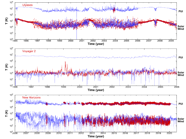
Much of our current understanding of turbulence in the outer heliosphere and VLISM relies on the Voyager (V1, V2), Interstellar Boundary Explorer IBEX, and New Horizons (NH) missions. Launched in 1977, V1 and V2 crossed the HP at 120 AU (in 2012 and 2018, respectively), and continue to provide us with unique in situ measurements in the heliosheath and VLISM.
Difficulties in the study of turbulence in these regions stem from the fact that one-dimensional in situ data cover just a tiny fraction of space, while the instruments onboard Voyager were not specifically designed to study turbulence in the outer heliosphere. Moreover, combined magnetic field and PUIs measurements are not available. In spite of this, the Voyager exploration resulted in truly remarkable discoveries, most of which being summarized in the papers constituting this volume. One of them is the observation of compressible turbulence in the heliospheric boundary regions (Burlaga et al., 2006a, 2015). The heliospheric community is eagerly expecting exciting new results before Voyagers lose their contact with Earth.
The properties of turbulence in the outer heliosphere are very much different from those in the near-Earth environment. For this reason, further observational and theoretical studies are expected to shed light onto the nature of turbulence in space plasmas.
The review is organized as follows. Section 2 is focused on turbulence in the distant, supersonic SW and summarizes the principal methods of its analysis. Section 3 gives an overview of the turbulence transport models and their predictions, and describes the efforts undertaken to couple them with global, 3D models. Section 4 describes turbulence and magnetic structures observed by V2 across the HTS and their implications for the transport of energetic particles. The observational evidence and our current understanding of turbulence, time-dependent structures and related scales in the IHS and VLISM are reviewed in Sections 5 and 6, respectively. Finally, Section 7 provides a brief overview of the as yet unsolved problems involving magnetic reconnection in these regions. Our conclusions are formulated in Section 8.
2 Evidence of turbulence in the distant supersonic solar wind
The turbulent dynamics of the solar wind beyond 10 AU can best be described as an evolution of what is seen at 1 AU with the addition of a significant driving source in the form of waves excited by newborn interstellar pickup ions (PUIs). We can examine what has been learned from studies of 1 AU observations as they form the bulk of solar wind turbulence studies for the purpose of obtaining a better understanding of turbulence beyond 10 AU.
Turbulent dynamics is studied via data analysis using four separate analysis methods, i.e. (i) comparing the form of the power spectrum to predictions, (ii) third-moment predictions for the cascade rate, (iii) comparison of both above rates to spatial gradients and/or transport theory, and (iv) multi-s/c techniques.
Predictions for the power spectrum based on specific theories of the nonlinear dynamics result in a testable prediction as well as an associated energy cascade rate through the inertial range that equals the heating rate. This can be augmented by other spectral analyses that are related to features such as helicity, polarization, etc. Single-spacecraft third-moment calculations are based on fewer assumptions of the underlying dynamics and give a rate of energy cascade that is largely independent of dynamics apart from an assumption of geometry (the statistical distribution of wave vectors in 3D space). Comparison of the computed energy cascade rate to the rate of heating as obtained either from statistical spatial gradients of the plasma temperature or transport theory yield a measure of the correctness of the computed energy cascade rate. Multi-spacecraft techniques that include, but are not limited to, -telescope methods attempt to resolve the underlying distribution of wave vectors and assign dynamics to their evolution.
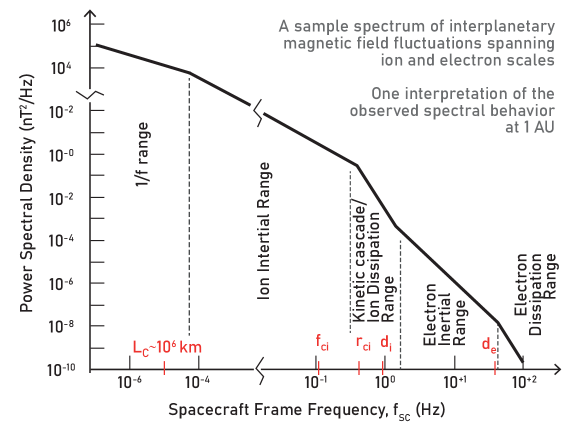
The power spectral density (PSD — or simply the spectrum, ) of SW turbulence can be described as having five subranges with (approximate) power law behavior , where is the spectral index. Figure 1 illustrates this. At the lowest frequencies where is the frequency as measured in the spacecraft frame and is the correlation scale (Matthaeus et al., 1999; Smith et al., 2001, 2006b), the spectrum consists of unprocessed energy that originates in the acceleration region (Matthaeus et al., 1983, 1986). By definition, the lifetime of these fluctuations is longer than the age of the SW plasma (causality condition). At the intermediate frequencies where is the scale where dissipation sets in - typically the larger of the Larmor radius and the ion inertial length - (Leamon et al., 1998a; Markovskii et al., 2008; Smith et al., 2012; Woodham et al., 2018; Pine et al., 2020a), the evolution of the fluctuations is (almost) energy-conserving and the nonlinear dynamics of the turbulence remakes the energy so as to transport the energy to smaller scales (Kolmogorov, 1941b; Matthaeus and Goldstein, 1982; Leamon et al., 1998a). This is the so-called inertial range where the fluctuations are unpolarized and the power spectra indices are reproducible (Matthaeus and Goldstein, 1982; Pine et al., 2020b). The ion “dissipation range” is described as and at 1 AU it is generally characterized as a steepening of the power spectrum starting at Hz. Various terminologies have been used in the literature. Our notation refers to the onset of dissipation effects at sub-ion scales. It is consistent with recent results that turbulent energy conversion into internal energy turns on at sub-ion scales, in weakly collisional plasmas (e.g., Matthaeus et al., 2020; Matthaeus, 2021, and references therein) and it agrees with observations. It has been shown that the rate of heating thermal protons in the SW is in good agreement with the rate of energy transport through the spectrum. What we know is that the spectrum steepens at a predictable scale, and that the polarization then changes in keeping with resonant dissipation removing one of the polarizations. Observations suggest that there must be dissipation of most of the transported turbulent energy in order to match in situ heating. However, the cross-scale transfer is not precluded in the kinetic regime. In fact cascade phenomenology in the ion kinetic regime is predicted by a number of studies (e.g., Howes et al., 2011). However, many aspects of how the cascade operates in the kinetic regime are unknown, especially in the outer heliosphere. Interestingly, the steepness of the ion dissipation spectrum depends on the strength of the inertial range energy transport (Smith et al., 2006a) and is generally absent beyond AU (Pine et al., 2020a). At still higher frequencies there is an electron inertial range where the dynamics are supported by the thermal electrons until dissipation occurs (Bale et al., 2005; Alexandrova et al., 2008, 2009, 2012).
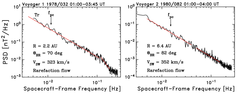
Figure 2 shows two typical examples of magnetic power spectra from the Voyager 1 & 2 spacecraft at 2.2 and 6.4 AU, respectively. Figure 2 (left panel) shows an example where the spectral break marking the onset of dissipation is evident at Hz. The flattening of the spectrum at Hz is most likely due to noise in the data rather than the onset of the electron inertial range. Figure 2 (right panel) shows an example where the spectral break is not observed. Analysis suggests that the onset of dissipation is resolved within the frequency range shown, but the spectral transport of energy through the inertial range is too weak to result in a observable break in the power spectrum when dissipation sets in.
As is frequently seen at 1 AU, the onset of dissipation is characterized by a bias of the polarization that can be interpreted to be a measure of the role of resonant dissipation (Leamon et al., 1998b; Hamilton et al., 2008; Pine et al., 2020a) and an increase in the relative amount of compressive fluctuations as measured by the spectrum of the magnetic field magnitude and parallel component.
0.7!
There are many properties of solar wind turbulence beyond 1 AU that are consistent with results obtained using 1 AU observations, including the observation of inertial range spectral indices falling within a consistent range of values. Broadband power spectra of plasma, magnetic field, and helicities have been computed in the MHD regime at 5 AU and 20 AU using V2 MAG and PLS data (Fraternale et al., 2016; Gallana et al., 2016; Iovieno et al., 2016; Fraternale, 2017). Special care has to be taken when analyzing and interpreting Voyager time series in the distant SW, due to the large fraction of missing data and the large noise-to-signal ratio at frequencies near ion scales. The cross and magnetic helicity analysis of V2 data at 20 AU by Iovieno et al. (2016) confirmed a tendency towards the reduction of cross helicity, consistent with model predictions of Matthaeus et al. (2004) and observations of Roberts et al. (1987). At large inertial scales ( Hz) speed fluctuations spectral indexes were found by Burlaga et al. (2003c) to drop from the Kolmogorov-like value () at 5 AU to at AU. This is the region where corotating interaction regions (CIRs) merge producing CMIRs where the plasma features pressure jumps of broad angular extent, shocks, and shock-like structures. Interestingly, the spectral index further decreases at larger distances AU, which was associated with the observed slowly evolving jump-ramp profiles of the SW speed. Consistently, the spectral indexes of magnetic field fluctuations in the same frequency range were found to vary between -1.8 and -2.5 (Burlaga et al., 2003b).
Looking at smaller scales in the inertial regime, magnetic field structures with quasi-2D, filamentary topology and multifractal statistics of increments are ubiquitous in the supersonic SW (e.g., Burlaga, 2001, 2004). As discussed by Vörös et al. (2006), both the local interaction and the cross-scale interaction between these structures and shocks play an important role in the dynamics of SW turbulence and the evolution of intermittency. In the inertial and dissipation regimes of turbulence, the distribution of magnetic field increments () is not Gaussian at frequencies higher than about the solar rotation frequency (e.g., Marsch and Tu, 1994; Sorriso-Valvo et al., 1999). Indeed, the q-Gaussian distribution (Gaussian core and fat power-law tails, Tsallis, 1988) was found to excellently fit the data (Burlaga et al., 2007), and is associated with intermittent behavior. A remarkable feature of turbulence in the distant SW is the significant decrease of intermittency observed by Burlaga et al. (2007) at 60 AU, (see details in Richardson et al. (2022), this volume), and recently further investigated by Parashar et al. (2019) and Cuesta et al. (2022). In these later papers the observed reduction of the small-scale intermittency of magnetic field increments with distance, out to 10 AU, is associated with the decreasing bandwidth of the inertial range with distance (effective Reynolds number scaling as ).
Another consistent property is the apparent dependence of the fluctuation anisotropy upon both the ambient plasma parameters, spectral intensity, and other turbulence properties (Leamon et al., 1998a; Smith et al., 2006a; Hamilton et al., 2008; MacBride et al., 2010; Pine et al., 2020c). There are two forms of fluctuation anisotropy that provide insight into the underlying dynamics. The first is the spectral ratio of and , the two diagonal components of the PSD perpendicular to the mean field. In a powerlaw region of the spectrum this ratio varies with the angle of mean field to the radial (observation) direction and provides insight into the fraction of energy associated with parallel and perpendicular wave vectors (Bieber et al., 1996). Efforts to extend this method beyond 10 AU have not been satisfactory (Pine et al., 2020c). The second type of anisotropy is the ratio of the energy of the perpendicular component relative to the parallel component that is a measure of the relative content of compressive fluctuations (Belcher and Davis, 1971).
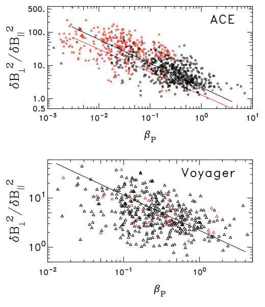
Figure 3 (top) shows the latter form of spectral anisotropy computed for 960 intervals of ACE observations at 1 AU averaged over the frequency range . Figure 3 (bottom) shows the spectral anisotropy computed for 438 intervals of V1 and V2 observations averaged over the spacecraft-frame frequency range where is the ion inertial scale ( is the Alfvén speed, is the mean field strength, is the thermal proton mass density, and are the proton cyclotron and plasma frequencies, respectively). This analysis has its roots in the general behavior of compressive waves. At the same time, a strong scaling of the same anisotropy is seen as a function of the ratio of the fluctuation level to the mean field strength. Figure 4 shows the analysis of the same ACE and Voyager spectra as a function of the square root of the integral of the power spectrum over the prescribed frequency range (the fluctuation amplitude) divided by the mean field strength. This analysis has its roots in nearly incompressible turbulence theory (Zank and Matthaeus, 1992b, a, 1993). At present there is no resolution to the ambiguity presented in these two figures as both the proton beta and are themselves strongly correlated. However, they point to the fundamental physics on which the nonlinear dynamics of turbulence is built.
0.717!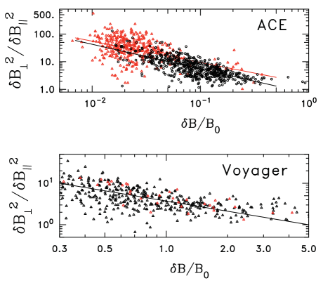
Analyses based on the use of data from a single spacecraft suffer from uncertainty derived from the necessary application of the Taylor Frozen-In-Field assumption (Taylor, 1938). This results in ambiguity regarding the actual orientation of the wave vector as it projects onto the SW velocity. The continuum of wave vectors that possess the same projection represent significantly different nonlinear dynamics leading to ambiguity in the resulting analysis. Assumptions are often made based on characteristics of the spectrum (Bale et al., 2005; Alexandrova et al., 2008) and the resulting interpretations are often debated, but this represents a major source of uncertainty in many SW turbulence analyses. There are statistical tests that attempt to address this question using single-spacecraft data (Bieber et al., 1996; Leamon et al., 1998a; Dasso et al., 2005; Hamilton et al., 2008; Pine et al., 2020c), but there also exist competing dynamics that can mask the effects of the nonlinear dynamics.
The leading theories for the inertial-range total energy power spectrum include the and the scaling for wavenumbers perpendicular to the mean magnetic field. The former is commonly referred to as the Iroshnikov–Kraichnan (IK) scaling due to their seminal works (Iroshnikov, 1964; Kraichnan, 1965). Using weak turbulence arguments, they first recognized the importance of the large-scale magnetic field in the turbulence dynamics, i.e., the role of interacting Alfvén-wave packets propagating in opposite directions. The rigorous weak turbulence theory predicts a scaling (Galtier et al., 2000; Schekochihin et al., 2012), but the IK spectral scaling is recovered for the case of strong, globally isotropic, Alfvénic turbulence, if the time scale that determines the energy transfer is given by the Alfvén time scale. Naturally, the original isotropy assumption can be difficult to justify when there is a mean field and the IK model is no longer heavily used for these cases. The scaling (Kolmogorov-type, after Kolmogorov, 1941b) arises in MHD in strong anisotropic turbulence scenarios when the nonlinear timescale determines the energy transfer (Goldreich and Sridhar, 1995, GS). Later theoretical developments for strong turbulence (Boldyrev, 2005, 2006) attempted to reconcile GS-style arguments with a scaling, since both were claimed to be observed in data and numerical simulations (e.g., Maron and Goldreich, 2001), despite the undeniable difficulty to discriminate between them. The model of Boldyrev (2006) is based on a scale-dependent “dynamic alignment” of the polarizations of magnetic- and velocity-field fluctuations, according to which both the and scaling can be obtained, depending on the anisotropy level. We note that the Boldyrev strong turbulence scaling is unrelated to the IK scaling (or at least not directly related). Additionally, a (distinct) scaling is also derived for the fast-mode cascade in compressible MHD turbulence (e.g., Cho and Lazarian, 2002). Though observations and more recent simulations tend to favor the scaling (e.g., Beresnyak, 2012), the question is still debated (see the extensive reviews of Zhou et al., 2004; Beresnyak and Lazarian, 2015), and many papers report one or the other in their study of specific events.
The energy cascade rates vary significantly between the theories within this range of spectral predictions (Leamon et al., 1999; Vasquez et al., 2007; Smith, 2009; Matthaeus and Velli, 2011). One example of such predictions is the MHD generalization of traditional hydrodynamics (Kolmogorov, 1941b; Leamon et al., 1999):
| (1) |
where is the total inertial range power spectrum (magnetic + kinetic), is the rate of turbulent energy transport through the inertial range, and is the wave vector magnitude. Evaluation of the constant to reach agreement with SW observations results in an expression for :
| (2) |
where is the measured power spectrum as a function of frequency, is the bulk SW speed in units of km s-1, and is the proton number density in units of cm-3. The above expression has roots in the hydrodynamic analog first used by Kovasznay (1948), and is based on dimensional arguments.
When applying these theories to inferred heating rates, it is assumed that the energy that passes through the inertial range is converted into heat by various kinetic processes with the bulk of the energy going into thermal protons and a smaller fraction being absorbed by heavy ions and thermal electrons. Using the published radial dependence of Helios thermal proton observations, Vasquez et al. (2007) concluded that the MHD extensions of hydrodynamic theory (Kolmogorov, 1941b; Leamon et al., 1999; Matthaeus and Velli, 2011) provided a better description of the observed heating rates from 0.3 to 1 AU once the universal constant was adjusted. They also obtained the following scaling for the average thermal proton heating rate as a function of heliocentric distance:
| (3) |
in units of J kg-1 s-1, is the temperature of thermal protons in Kelvin, and is the heliocentric distance in AU.
Third moments, or third-order structure function, theory originates with hydrodynamics (Kolmogorov, 1941a). The great advantage of applying this formalism to MHD is that the derivation and application does not make use of any particular model of the dynamics (Politano and Pouquet, 1998a, b). In this way, it provides a formulation for the rate of energy cascade through the inertial range that is independent of any specific turbulence model. Instead, the MHD equations are combined with assumptions regarding compressibility, stationarity, homogeneity, and underlying geometry (i.e. rotational symmetry). The combined assumptions of incompressibility, stationarity, and homogeneity along with specific assumptions of geometry produce expressions that are general and applicable to data from single spacecraft without further assumption (Politano and Pouquet, 1998b, a; MacBride et al., 2015; Sorriso-Valvo et al., 2007; Marino et al., 2008, 2011, 2012; MacBride et al., 2008; Stawarz et al., 2009; Coburn et al., 2012, 2014, 2015; Hadid et al., 2017; Smith et al., 2018). Third-moment theory does not require specific power spectral forms or the assumption of a detailed nonlinear dynamic. Compressibility leads to expressions that include some terms that cannot be evaluated using single spacecraft data (Galtier, 2008; Carbone et al., 2009; Hadid et al., 2017; Hellinger et al., 2018). The de Kármán–Howarth equation derived for incompressible MHD reads (Politano and Pouquet, 1998b):
| (4) |
where
| (5) | |||||
| (6) |
Here are the Elsässer field fluctuations (Elsässer, 1950, with the plasma speed, the magnetic field, the proton mass density, the magnetic permeability, and , etc) and denotes the rate of cascade of . The total energy cascade rate per unit mass, , is given by
| (7) |
When an assumed distribution of wave vectors (e.g., 1D, 2D, or isotropic) is applied to the divergence , expressions are obtained that are applicable to single spacecraft observations. Assuming isotropy, for example, we can write:
| (8) |
where denotes the radial component, is the time lag in the data, and denotes the ensemble average.
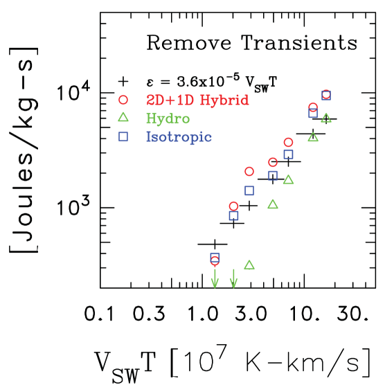
Third-moment theory has been shown to accurately reproduce 1 AU heating rates in both the compressible and incompressible forms. Figure 5 is taken from Stawarz et al. (2009) showing the result of analyzing 10 years of ACE data and compares the average energy spectral transfer rate (assumed to be the thermal proton heating rate) using the third-moment formalism under the isotropic and combined 2D+1D hybrid geometry assumptions and compares these results to the Vasquez et al. (2007) prediction of Eq. (3) and to the familiar hydrodynamic form.
Third-moment analyses using spacecraft data beyond 10 AU are ongoing, but unpublished at this time. Turbulent transport theory can be used to propagate the turbulent dynamics into the outer heliosphere and obtain predictions for the turbulence level, temperature and heating rate, correlation scale, and cross-field correlation most notably called the “cross helicity” or “imbalance”. The predictions of transport theory can then be compared to fluctuation levels and thermal proton heating rates which are assumed to be the same as the local energy cascade rate as obtained from theories based on the power spectrum.
It is widely assumed that the PUIs generate turbulence in the distant SW due to their initial ring-beam velocity distributions which are unstable to the excitation of Alfvén/ion cyclotron modes and should evolve into a spherical, filled-shell distribution (Wu and Davidson, 1972; Vasyliunas and Siscoe, 1976; Lee and Ip, 1987; Gary and Madland, 1988; Gary, 1991; Zank, 1999b). The fluctuation energy produced by PUIs adds to the existing turbulence and is assumed to dissipate at small spatial scales by supplying the energy to SW protons and electrons via a turbulent cascade. Therefore, low-frequency magnetic turbulence heats the SW plasma and results in a non-adiabatic SW temperature profile and a slow temperature increase beyond AU (e.g., Williams et al., 1995; Matthaeus et al., 1999, 2004; Smith et al., 2001, 2006b; Isenberg et al., 2003; Isenberg, 2005; Chalov et al., 2006; Breech et al., 2008, 2009; Isenberg et al., 2010; Gamayunov et al., 2012).
It follows that in transport theory for SW fluctuations a significant element is the inclusion of this outside energy source associated with wave excitation by newborn interstellar PUIs. Indeed, it becomes the primary source of energy that drives the turbulence beyond 10 AU. This source term becomes critical to reproducing the observed turbulence and heating levels beyond 10 AU (Matthaeus et al., 1999; Smith et al., 2001; Breech et al., 2008; Oughton et al., 2011; Adhikari et al., 2017) and can be compared with the theories of interstellar neutral ionization and associated wave excitation. Further details on PUI waves are provided in Sokół et al. (2022) in this volume.
3 Modeling of the supersonic solar wind with turbulence transport
Numerous problems in space physics and astrophysics require a detailed understanding of the transport and dissipation of low-frequency turbulence in the expanding inhomogeneous magnetized solar wind plasma. For instance, knowledge of spatial distribution of turbulence intensity is an important input for computations of energetic particle propagation throughout the heliosphere. Coupling global heliospheric models and turbulence transport models provides not only mean-flow plasma and magnetic field parameters, but also the turbulence quantities, which makes them useful also for calculation of diffusion coefficients and modulation of galactic cosmic rays (GCRs) (see, e.g., Florinski et al., 2013a; Engelbrecht and Burger, 2013; Wiengarten et al., 2016; Chhiber et al., 2017; Engelbrecht, 2017; Zhao et al., 2018). This topic is reviewed by Engelbrecht et al. (2022) in this volume.
Transport models for solar wind fluctuations in the supersonic and super-Alfvénic SW have advanced considerably since the presentation of the initial 1D Wentzel–Kramers–Brillouin (WKB) approach with prescribed (inhomogeneous) background fields (Parker, 1965). The WKB theory (see also Tu et al., 1984) can only describe the evolution of linearly interacting modes, whose typical time scale is much shorter than that of the overall cascading. The more general turbulence transport models are based on a few statistical parameters that characterize the turbulence in the supersonic SW. Most of them build upon the Kármán–Howarth kind of one-point closure models for local evolution of turbulence (de Karman and Howarth, 1938). In the theory, a phenomenological description of the turbulent cascade is merged with transport equations obtained from a scale-separated decomposition (see Eq. 9) of the MHD equations (Zhou and Matthaeus, 1989; Marsch and Tu, 1989; Zhou and Matthaeus, 1990; Tu and Marsch, 1993) which supports coupling of the small-scale (turbulence) quantities to the large-scale quantities, e.g., the mean SW velocity , magnetic field , and mass density (for a review see Oughton and Engelbrecht, 2021).
In the turbulence transport theory, the Elsässer variables represent propagating modes moving parallel () and antiparallel () to , provided that the wavevectors involved satisfy (e.g., Tu et al., 1984; Zhou and Matthaeus, 1990, 1990; Beresnyak and Lazarian, 2015). The interaction between these counter-propagating modes leads to the generation of quasi-2D turbulence in a plane perpendicular to the mean magnetic field, which by direct energy cascade eventually heats the SW. The time scales of such nonlinear interactions are , where are the correlation lengths associated with the turbulent Elsässer energies, while the time scale of linear interaction is . The characteristic time scale of the turbulent cascade (or spectral transfer time) can be expressed as , where is the triple-correlation lifetime (Matthaeus and Zhou, 1989). The evolution of incompressible ideal MHD fluctuations in the presence of (scale-separated) inhomogeneous large-scale fields can be written in the following form (Zhou and Matthaeus, 1990),
| (9) |
where are the nonlinear terms, and are external sources. Constructing the moments of Elsässer variables from Eq. 9 introduces terms like , which are regarded as MHD analogs of the hydrodynamic Reynolds stress. Due to the presence of terms, the backward and forward propagating modes interact through the small-scale fluctuations, large-scale SW speed and magnetic field.111Some definitions and nomenclature that will be used throughout in this paper are given: the Elsässer energies , total turbulence energy density, , the residual energy and its normalized value, , the normalized cross helicity , the Alfvén ratio . and are the turbulent kinetic energy and magnetic energy densities in Alfvén units, respectively.
Most of the fluctuation energy is associated with the ‘energy-containing range’ of scales and transport models that follow energy-containing range quantities are of interest. These quantities include the Elsässer energies , the residual energy (aka energy difference) , and characteristic lengthscales for each of these.
A rough timeline of the development of these models is given here, and we note that they usually need to be solved numerically. Matthaeus et al. (1994) used the Reynolds decomposition approach to develop a four-equation transport model for , , and a single characteristic lengthscale. So-called ‘mixing’ effects, due to gradients of the large-scale SW velocity and magnetic field, couple the turbulence quantities to each other and support for generic driving of the fluctuations is also included. Zank et al. (1996a) considered a zero cross helicity special case of this model with two dynamical equations (for the magnetic energy and its lengthscale) while also including turbulence sources due to shear, compression, and PUI heating. Their model was able to describe the observed radial decay of turbulence reasonably well. Matthaeus et al. (1999) extended this to include a transport model for the proton temperature with proton heating by PUIs, and a simple closure for local anisotropic MHD turbulence, and found excellent agreement with V2 data from 1 to 60 AU. The effects of magnetic energy dissipation in the proton temperature were included by Smith et al. (2001). Later, Smith et al. (2006b) improved the description of the PUI source term using the formalism of Isenberg et al. (2003) (see Eqs. 10–12). A transport theory including cross helicity was formulated by (see also Matthaeus et al. 1994 Matthaeus et al., 2004) and further developed by Breech et al. (2005) and Breech et al. (2008). Using the model equations of Smith et al. (2001) and Isenberg et al. (2003), Ng et al. (2010) investigated the effect of IK cascade, finding similar or even higher heating rates than that obtained by using the Kolmogorov cascade. Later models included the electron heating (Breech et al., 2009) and the deceleration of SW by PUIs (Isenberg et al., 2010). Building on Breech et al. (2008), Oughton et al. (2006, 2011) developed an anisotropic two-components model where PUIs can directly influence the quasi‐parallel wavenumber fluctuations.
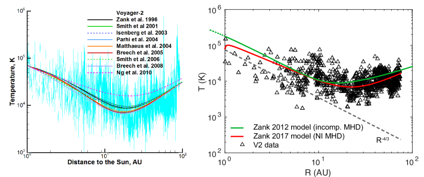
The above models are applicable to the super-Alfvénic SW () under a number of assumptions and approximations, reviewed by Oughton and Engelbrecht (2021). A six-equation incompressible MHD turbulence model applicable also to sub-Alfvénic flows was developed by Zank et al. (2012) by introducing separate correlation lengths associated with the forward- and backward-propagating modes (cf. Matthaeus et al., 1994). Adhikari et al. (2014) investigated the effects of solar cycle variability on the Zank et al. model, and Adhikari et al. (2015) obtained turbulence quantities at distances up to 100 AU. With selection of appropriate shear constants, and boundary values, these transport theories have been able to account quantitatively for Helios and Ulysses proton temperature observations as well as Voyager data from 1 to more than 60 AU (Zank et al., 1996a; Matthaeus et al., 1999; Smith et al., 2001, 2006b).
There are recent models that also support a 3D heliosphere with dynamically evolving background fields coupled to fluctuation quantities (e.g., Kryukov et al., 2012; Usmanov et al., 2012, 2014, 2018; Wiengarten et al., 2016; Shiota et al., 2017). Attempts to include the heliosheath and VLISM in the global models have also been presented (e.g., Usmanov et al., 2016; Fichtner et al., 2020). Usmanov et al. (2014) improved their previous model by using an eddy viscosity approximation for the Reynolds stress tensor and the mean turbulent electric field. They demonstrated that the effect of eddy viscosity and, correspondingly, of velocity shear on the mean-flow parameters manifests itself in the increased temperatures of SW protons. The turbulence energy and the correlation length are notably increased and the cross helicity decreased, especially near transitions between fast and slow SW flows.
Simulation results based on these models give encouraging, if incomplete, agreement with outer heliosphere spacecraft observations (Marsch and Tu, 1990; Williams and Zank, 1994; Williams et al., 1995; Richardson and Smith, 2003; Richardson et al., 1995, 1996; Usmanov et al., 2016).
A relatively simple steady-state transport model (Smith et al., 2001, 2006b; Pine et al., 2020d) can be written as equations for the total average fluctuation energy density,
| (10) |
the similarity scale,
| (11) |
and the proton temperature,
| (12) |
The parameters of the theory are heavily constrained by observations.
The above citations use , , , , , and (Matthaeus et al., 1999). It is important to note that represents the fluctuation energy in the large-scale, or energy-containing, range of scales. The inertial range is not explicitly represented here. However, terms that scale as represent the loss of energy in coherent turbulent fluctuations due to the spectral transport of energy from large to small scales and the conversion of that energy into heat. At large Reynolds numbers this spectral transport will involve energy transfer through an implied inertial range. The term represents expansive cooling. The term represents the rate of energy injected into the turbulence via wave energy excitation by newborn interstellar pickup ions. This can be modeled using the rate of ion production obtained from the analytic Warsaw Test Particle Model (aWTPM) and the numerical Warsaw Test Particle Model (nWTPM) codes (e.g., Bzowski, M. et al., 2013; Sokół et al., 2015, 2019), or global MHD plasma/ kinetic neutrals simulations, reviewed by (Kleimann et al., 2022) in this volume. The analysis of Voyager data from launch through 1990 described below uses a photoionization rate model determined from series of solar EUV proxies, like F10.7, MgII core-to-wing index, and CELIAS/SEM correlated with the solar EUV measurements from TIMED (Bzowski, M. et al., 2013; Bochsler et al., 2013; Sokół et al., 2019). The resulting ion production rates can be combined with the theory of wave excitation by pickup ions (Lee and Ip, 1987) to produce an estimate for .
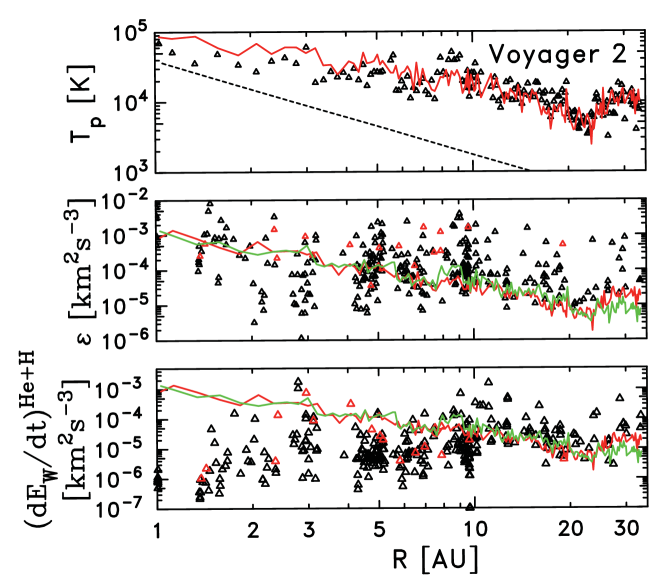
The top panel of Fig. 6 from Pine et al. (2020d) shows the result of comparing the predictions for the thermal proton temperature as derived from the above transport model (red line) with the measured average proton temperature (symbols). The dashed line represents adiabatic expansion from 1 AU. The evidence for some form of in situ heating is undeniable. Transport theory accurately reproduces the observed average temperature of SW protons. Figure 6 (middle) compares the rate of energy dissipation derived from the transport model (red line) and Eq. 3 (green line) against the rate of heating obtained from Eq. 2 as applied to magnetic spectra from 327 intervals of V2 observations. Although agreement between transport theory and Eq. 3 is good, the results derived from the magnetic spectra do show a broad distribution about the predictions for the average heating rate. This is partly due to the natural variation of the turbulence, partly due to the fact that the data intervals were selected to be used as controls in the analysis of waves due to PUIs, and partly due to rejection of low spectral levels with evidence of instrument noise in the data. Figure 6 (bottom) compares the rate of thermal proton heating obtained from the transport model (red line) and eq. 3 (green line) against the rate of wave energy excitation by newborn interstellar pickup and (symbols) using the above formalism applied to the same data intervals as the middle panel. Wave excitation by newborn interstellar PUIs becomes the primary source of energy that drives the turbulence beyond 10 AU.
PUIs are thermodynamically different from thermal protons (Vasyliunas and Siscoe, 1976; Isenberg, 1986). While their number density is relatively low, their impact on the SW, including its heating and gradual deceleration, is significant. The very high effective temperature (107 K) of pickup protons makes them the dominant component of the thermal pressure in the distant SW (Burlaga et al., 1996). Speaking of global heliosphere numerical simulations, the most obvious problem with adopting the single-fluid description for SW plasma is that it implies an immediate assimilation of the newborn PUIs with thermal SW protons. As a result, single-fluid models predict a steep increase of the plasma temperature with radius beyond 10 AU, where the pickup protons play a major role. A modest increase in the temperature of SW protons is indeed present in V2 data beyond 30 AU. However, the steep rise predicted by single-fluid models is in obvious disagreement with V2 observations. PUIs should, in principle, be modeled as multiple populations (Malama et al., 2006). In the fluid approach, it is then important to model PUIs by a separate energy equation, as shown by Isenberg (1986) and further elaborated by Zank et al. (2014a). After the first 1D fluid model of Isenberg (1986), 3D models were developed by Usmanov and Goldstein (2006) and Detman et al. (2011), with PUIs treated as a separate fluid, but including only the supersonic SW region. Later, the effects of pickup protons as a separate fluid were included in the 3D heliospheric models of Pogorelov et al. (2016) (MS-FLUKSS code). For details on global models, see Kleimann et al. (2022).
The approach used by Usmanov et al. (2014, 2016) to modeling turbulence effects in the SW follows the transport theory, which describes the effects of transport, cascade, and dissipation of incompressible MHD turbulence. The time-dependent turbulence transport equations read
| (13) |
| (14) |
| (15) |
where and are the Kármán–Taylor constants. The term is the average induced fluctuation electric field, and is a function of cross helicity that modifies the nonlinear decay phenomenology if . is the Reynolds stress tensor, and and are source terms due to charge exchange and photoionization. This model assumes the local incompressibility of fluctuations, and a single characteristic lengthscale, .
Having their focus on the heliospheric interface region, the existing global models of the outer heliosphere typically employ simplified patterns for the SW and interplanetary magnetic field parameters at their inner boundaries, which are usually placed between 10 and 50 AU. The most frequent assumption is that the SW is spherically symmetric (e.g., Washimi and Tanaka, 1996; Pogorelov and Matsuda, 1998; Ratkiewicz et al., 1998; Opher et al., 2003; Izmodenov et al., 2005; Ratkiewicz and Ben-Jaffel, 2002; Borrmann and Fichtner, 2005; Pogorelov et al., 2006; Opher et al., 2009; Izmodenov et al., 2014). Latitudinal variations at the inner boundary consistent with Ulysses observations of the bimodal SW near solar minimum have been included, e.g., by Pauls and Zank (1997); Linde (1998); Pogorelov et al. (2013b); Provornikova et al. (2014). The first global heliospheric models that used observations of solar magnetograms to extrapolate time-dependent inner boundary conditions at 0.1 AU is that of Detman et al. (2011). Later, Usmanov et al. (2016) were able to carry solar corona/SW computations from the coronal base.
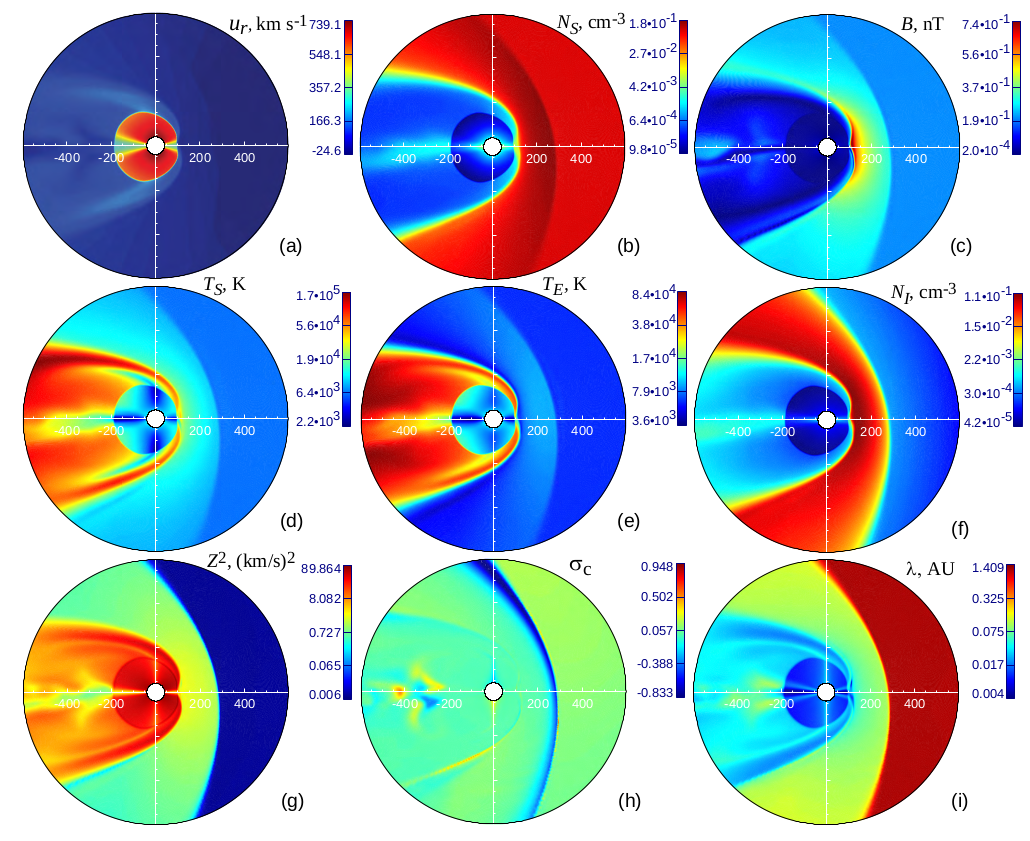
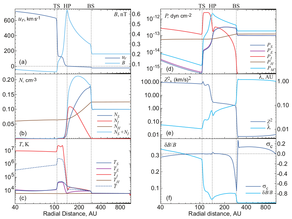
Usmanov et al. (2016) further extended their three-fluid SW model by including the heliospheric interface region. This is the first attempt to include turbulence effects in global simulations including the heliosheath and the VLISM. They constructed such a 3D model taking into account turbulence transport and separate energy equations for thermal protons, electrons, PUIs, and interstellar hydrogen, and then, using this model, studied the formation of the heliospheric interface region. We note here that the Usmanov et al. (2016) turbulence model is applicable to both super-Alfvénic and sub-Alfvénic flows. A shortcoming of the model, as stated by the authors, is that it is suitable for incompressible turbulence, while compressibility is a prominent feature of turbulence in the inner and outer heliosheath. Modeling of these regions still represents a major challenge. Figures 7 and 8 show some results from Usmanov et al. (2016) for plasma, magnetic field and turbulence parameters in the outer heliosphere.
A turbulence model for the supersonic SW (Breech et al., 2008) has also been included in a global, 3D data-driven simulation by Kryukov et al. (2012), assuming spherically symmetric SW at the inner boundary. While the data-driven, time-varying simulation produced mostly realistic SW variations along the V2 trajectory out to 80 AU, there were still some systematic discrepancies during certain periods when the assumption of spherically symmetric SW using near-Earth data was clearly inappropriate away from the ecliptic plane. To alleviate such discrepancies, Kim et al. (2016, 2017b) introduced spatial variations across the model inner boundary using Ulysses data as constraints, and the results showed excellent agreements with Voyager and NH data. Subsequently, Kim et al. (2017a) used the improved boundary conditions along with the Breech et al. (2008) turbulence model to reproduce the temporal/spatial variations of SW and PUI between 1 and 80 AU. The simulated SW and PUI temperatures are shown compared with the Ulysses Intriligator et al. (PUI from 2012), V2 (SW only), and NH data (PUI from McComas et al., 2021) in Fig. 9.
Another class of turbulence transport models is based on the nearly incompressible (NI) MHD phenomenology (Zank and Matthaeus, 1992b, 1993; Hunana and Zank, 2010; Zank et al., 2017a). In contrast to incompressible MHD models of the fluctuations, NI MHD theory assumes that the fluctuations are weakly compressible. The compressible MHD equations are separated into a set of core incompressible equations and a weakly compressible fluctuating part. Core equations are obtained using the bounded time derivatives method given by Kreiss (Kreiss, 1980), a constraint that is imposed to ensure that the fast-timescale magnetoacoustic waves vanish. The normalized equations for the fluctuations are expanded with respect to the low Mach number, then terms of similar order are collected (Zank and Matthaeus, 1992b, 1993). Zank and Matthaeus (1993) considered three plasma beta regimes, , , and , respectively (). They showed that the leading order incompressible MHD description is fully 3D for , while it reduces to 2D in the plane perpendicular to the mean magnetic field for and . Higher-order corrections to the leading-order NI fluctuations are fully 3D. Based on the observed values of the Mach number (NI expansion parameter) Zank and Matthaeus (1993) predicted that SW turbulence in the or regimes is a superposition of the dominant () 2D turbulence and a minority () slab turbulence.
Incompressible MHD turbulence models for SW fluctuations are formally applicable in the high plasma beta regime () (although Squire et al., 2017, suggest, based on 2D hybrid simulations, that a weakly collisional high beta plasma can possess a self-induced pressure anisotropy not contained in the standard MHD closure) while the NI MHD turbulence model of Zank et al. (2017a) is applicable in the low-beta regime () or when . An important and practical distinction between the description and the and descriptions is that the latter allows for a clear decomposition into a distinct majority quasi-2D turbulence component and a distinct minority slab turbulence component that responds dynamically to the majority component. This is the theoretical underpinning of the well-known 2D+slab model (e.g., Bieber et al., 1996; Forman et al., 2011). By contrast, the incompressible description can allow for both quasi-2D and slab components but now on an equal footing and both dynamically coupled, for which descriptions such as critical balance (Goldreich and Sridhar, 1995) or 2D + wave-like (Oughton et al., 2011) have been developed. This renders the study of anisotropy throughout the heliosphere (Adhikari et al., 2017), provided the plasma beta regime is appropriate, rather more straightforward than use of the incompressible MHD model, provided in this case that . In addition, according to incompressible MHD model, turbulence turns off for the unidirectional Alfvén waves (in the homogeneous case), while it is not so in the NI MHD model (Adhikari et al., 2019). The model was able to reproduce the recent finding Telloni et al. (2019) that the unidirectional Alfvén wave can exhibit a Kolmogorov-type power law (Zank et al., 2020; Zhao et al., 2020b).
In the NI MHD phenomenology for a or plasma, the total Elsässer variables can be written as a summation of the majority quasi-2D and a minority NI/slab Elsässer variables, i.e., , where and (Zank et al., 2017a). Here, “” denotes the quasi-2D turbulence, and “*” the NI/slab component. The transport equations for the quasi-2D Elsässer fields fluctuation read (Zank et al., 2017a),
| (16) |
The difference between Eq. 9 and Eq. 16 is that the latter describes the convection of locally quasi-2D Elsässer variables, and does not include Alfvén propagation effects. The NI MHD approach is suitable for studying turbulence in SW, which is also supported by Zhao et al. (2020a) and Chen et al. (2020), who found several quasi-2D structures in SW, namely magnetic flux ropes. In addition, pressure-balanced structures (PBSs) or flux tubes (Burlaga, 1968, 1995; Vellante and Lazarus, 1987; Bavassano and Bruno, 1991; Borovsky, 2008; Sarkar et al., 2014), are commonly observed in the SW, are equilibrium solutions of NI MHD (Zank and Matthaeus, 1992b). PBSs/flux tubes are highly dynamical structures in the presence of quasi-2D turbulence (Zank et al., 2004). Zank et al. (2012) developed 6 coupled turbulence transport equations by taking moments of Eq. 9, and Zank et al. (2017a) developed 12 coupled quasi-2D and NI/slab turbulence transport equations to describe the transmission of energy in forward and backward propagating modes, residual energy, and the corresponding correlation lengths.
Most of the turbulence transport models mentioned in this section address the SW proton heating. Figure 10 (left panel), confronts the SW proton temperature measured by V2/PLS (blue line) with the result from different turbulence models implemented in a global, 3D unsteady simulation of the heliosphere. The proton temperature equation can be expressed as
| (17) |
where is a polytropic index, and is a turbulent heating term derived from a von Kármán–Taylor phenomenology (de Karman and Howarth, 1938). For example, the heating term using can be expressed as (Verdini et al., 2010; Zank et al., 2012; Adhikari et al., 2015),
| (18) |
where is a constant. Inside the square brackets of Equation (18), the first term is the nonlinear dissipation term corresponding to the energy in forward propagating modes, and the second term the nonlinear dissipation term corresponding to the energy in backward propagating modes. In Verdini et al. (2010), their Eq. (5) denotes the heating term, which was derived by using the nonlinear dissipation terms corresponding to the energy in forward and backward propagating modes. The first and second terms inside the square brackets of Eq. (18) are larger than that of Verdini et al. (2010), resulting in a larger heating rate, and therefore a larger SW temperature. In Adhikari et al. (2015), this is slightly ameliorated by the inclusion of the residual energy term.
Using Eq. 17 and Eq. 18, Adhikari et al. (2015) investigated the heating of SW plasma from 0.29 AU to 100 AU. Similarly, Adhikari et al. (2017) studied the proton heating from 1 AU to 75 AU using the NI MHD turbulence model (Zank et al., 2017a). The temperature profile from these two models is shown in Fig. 10 (right panel). The stream-shear source is found to be important within 4–5 AU, while the PUI-related turbulent source term is important beyond the ionization cavity boundary at AU. These sources drive turbulence throughout the heliosphere, and offset the decay of turbulence energy. The dissipation of turbulence, plus the additional driving of turbulence by the distributed heliospheric sources, yields a plasma temperature profile that is significantly different and of course higher than would be expected if only adiabatic cooling of the SW occurred (see the dashed curve in the right panel of Fig. 10). Naturally, adiabatic cooling is included in the SW models with turbulent heating. The increase of beyond 20 AU can be considered due to the presence of PUIs in the outer heliosphere. The results show that the theoretical proton temperature (solid red curve) obtained by using incompressible MHD and NI MHD turbulence models produce radial temperature profiles similar to the observed ones.
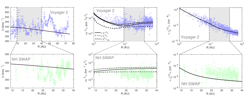
Pickup ions not only produce turbulence in the outer heliosphere, but also influence the SW properties. Zank et al. (2018) extended the classical models of Holzer (1972) and Isenberg (1986) by coupling a NI MHD turbulence model of Zank et al. (2017a) to a multi-fluid description of the SW plasma to properly examine the feedback between SW plasma heating, the modified large-scale SW velocity due to the creation of PUIs, and the driving of the turbulence by SW and interstellar PUI sources. The theoretical model of Zank et al. (2018) describes the evolution of the large-scale SW, PUIs, and turbulence from 1–84 AU. As shown in the left panel of Fig. 11, the theoretical SW speed (solid curve) gradually decreases with increasing heliocentric distance from 1 AU to 75 AU because the PUIs ions lead to the decrease of the momentum of the SW (see also, Richardson and Wang, 2003; Elliott et al., 2019). The theoretical speed is compared with V2 measurement (blue plus symbols, the top panel of Fig. 11) and NH SWAP measurements (green plus symbol, the bottom panel of Fig. 11).
The middle panel of Fig. 11 shows the quasi-2D, NI/slab, and total fluctuating kinetic energy with increasing heliocentric distance. The observed fluctuating kinetic energy exhibits quite a large scatter. The theoretical results are slightly higher than the observed NH SWAP values, although not significantly. This difference may be due to the fact that a single boundary conditions is used to compare with the V2 and NH data sets. The V2 observations are taken from 1983 - 1992 and those of NH from 2008 - 2017 for the radial heliocentric distance interval 11–38 AU, and the solar cycle observed by NH was much weaker than that observed over this distance interval by V2 (Lockwood et al., 2011; Zhao et al., 2014).

The variance of the fluctuating thermal plasma density is displayed in the right panel of Fig. 11. The theoretical fluctuating density variance shows good agreement with V2 observations (Fig. 11, top right panel), but underestimates the SWAP derived values (bottom right panel).
The PUI mediated model of Zank et al. (2018) predicted various turbulence quantities from 1–75 AU, as shown in Fig. 12, which also shows the corresponding values derived from V2 observations (see Adhikari et al. (2017)). These results are slightly different from the results predicted by Adhikari et al. (2017) assuming that the background radial SW speed is constant. Pickup ions lead to a gradual decrease of the SW speed, and the background density and magnetic field are modified accordingly. The radial dependence of the background flow, density, and magnetic field influences the evolution of turbulence throughout the heliosphere.
The energy density in the forward and backward Elsässer variables is displayed in the top two plots of Fig. 12. Here, the solid curves denote the majority quasi-2D component, the dashed curves the minority NI/slab component, and the dashed-dotted curves the quasi-2D + NI/slab component. The V2 observations are shown with blue plus symbols. Although the observed values have considerable dispersion, the predicted evolution in the forward, backward, and total Elsässer energy densities is consistent with observations. The normalized residual energy shows that both the theoretical quasi-2D and slab components decrease towards a magnetically dominated state within AU. However, as the PUI-driven turbulence becomes more important beyond the ionization cavity, increase towards zero with increasing heliocentric distance, i.e., turbulence becomes increasingly Alfvénic with . The normalized cross-helicity monotonically decreases to zero as distance increases, indicating that the energy flux in forward and backward propagating directions gradually becomes approximately equal, in accord with observations. Although PUIs in the outer heliosphere drive the NI/slab component of turbulence, it remains a minority component.
The fluctuating magnetic energy is displayed in the bottom panel of Fig. 12, indicating that theory and observations are consistent (Zank et al., 1996a; Matthaeus et al., 1999; Smith et al., 2001). Figure 12 provides a fairly complete characterization of the macroscopic (energy-containing scale) turbulence state throughout the heliosphere from 1–75 AU.
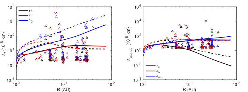
The correlation length is an important quantity in turbulence because it helps control the energy decay rates. Figure 13 shows the comparison between theoretical and observed correlation lengths as a function of the heliocentric distance. The theoretical 2D correlation length corresponding to the energy in forward propagating modes (solid black curve) and the energy in backward propagating modes (solid red curve) increases gradually from 1 AU to AU, and then flattens with distance. However, since there is no turbulent shear source in the NI/slab turbulence transport equation, the theoretical slab correlation length corresponding to the energy in both forward and backward propagating modes increases initially, and then decreases slightly due to the presence of pickup ions in the outer heliosphere. The theoretical 2D and slab correlation length of the residual energy increases gradually as distance increases. In the right panel of Fig. 13, the theoretical 2D and slab correlation length corresponding to the fluctuating kinetic energy and the cross-correlation between covariance of velocity and magnetic field fluctuations increase with distance. However, the opposite behavior is shown by the theoretical 2D and slab correlation length of the velocity fluctuations.
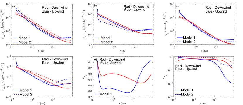
Recently, Adhikari et al. (2021) found that the turbulence property of the SW in the upwind direction is different from that in the downwind direction (along the Pioneer 10 trajectory), due to the different PUI production rates (Nakanotani et al., 2020). Therefore, the turbulent heating rates in the upwind and downwind directions are different. Figure 14 shows the turbulence cascade rates as a function of heliocentric distance, in both the upwind and the downwind directions, and compares results of two transport models. The solid curve corresponds to the turbulence cascade rate obtained from the turbulence transport theory (Model 1, incompressible MHD, Zank et al., 2012), and the dashed curve corresponds to the turbulence cascade rate obtained from the dimensional analysis between the power spectrum in the energy-containing range and the inertial range (Model 2, NI MHD, Adhikari et al., 2017). The turbulence cascade rates corresponding to the (fluctuation) Elsässer energies, magnetic energy,and kinetic energy all decrease gradually until AU and AU in the upwind and downwind directions, respectively. However, these turbulence cascade rates increase or flatten after AU in the upwind direction, and flatten or slowly decrease after AU in the downwind direction.
4 Turbulence at the heliospheric termination shock
The HTS plays a fundamental role in shaping the nature of turbulence in the inner heliosheath (Zank et al., 2006, 2010, 2018). In front of the HTS, turbulence consists of both preexisting SW fluctuations advected at the shock and locally generated fluctuations due to kinetic processes, and reflected fluctuations.
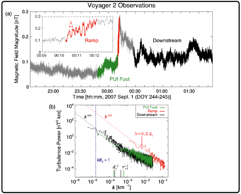
The third HTS crossing observed by V2 (hereinafter TS3, 2007 August 30, 84 AU; Stone et al., 2008) allowed to detect magnetic field fluctuations inside the shock structure (Burlaga et al., 2008). Since the shock thickness was estimated to be km (), these observations are only possible when using data of the highest resolution (0.48 s). Intense quasi-periodic fluctuations of with wavelength characterize the shock ramp (see Fig. 15). Spectral analysis of turbulence for this specific crossing were recently conducted by Zhao et al. (2019b) and Zirnstein et al. (2021). Figures 15–17 are reproduced from these studies.
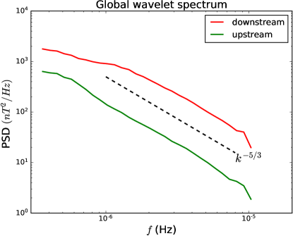
Zhao et al. (2019b) analyzed turbulence at relatively large scales using V2 data of 1 day resolution. Two intervals of 122 days were selected immediately upstream and downstream of the HTS. Power spectra are obtained from wavelet analysis, and show that magnetic turbulence on both sides exhibits a power law in the frequency range Hz, as shown in Fig. 16. The downstream spectrum is enhanced by a factor of with respect to the upstream spectrum.
Zirnstein et al. (2021) computed magnetic turbulence spectra using V2 data at the highest resolution of 0.48 s and considered short time intervals that include the shock’s PUI foot (green curves in Fig. 15), the ramp (red), and the downstream region (black), excluding the overshoot. The wavenumber range for the spectra shown in Fig. 15(b) include the gyroscale of PUIs with speed km s-1 (, in Fig. 15), the inertial length, and the Larmor radius of the thermal protons ( km in front of the HTS and 5800, 2300 km behind of it, respectively). The flatter upstream spectrum for km-1 may be due to the presence of noise from the fluxgate magnetometers. Interestingly, the turbulence power in the ramp is higher by a factor of as compared to the upstream spectrum. Zirnstein et al. (2021) investigate the effect of turbulence at the HTS on PUIs acceleration using a test-particle model. According to these simulations, the turbulence intensity observed by V2 at the PUI gyroscale upstream of the HTS, , is not sufficient to explain the observed suprathermal tail in the proton spectrum measured by IBEX at energies keV. Values similar to those extrapolated using the ramp spectrum, , may be necessary to explain IBEX observations.
Giacalone and Decker (2010) and Giacalone et al. (2021) investigated particle acceleration at the HTS up to energies of 50 keV via 2D hybrid simulations, and included background upstream SW turbulence in the form of random circularly polarized Alfvén waves with a Kolmogorov spectrum and normalized variance . Note that this intensity refers to the total background turbulence spectrum and is a function of the chosen value for the correlation length (0.17 AU). Their results suggest that large-scale turbulence () may also affect the particle distribution (see also Giacalone, 2005).
It should be noted that even without the background turbulence, fluctuations at the ion scale can be self-generated due to temperature anisotropy in the downstream region immediately behind the shock (e.g., Wu et al., 2009; Liu et al., 2010; Wu et al., 2010; Kumar et al., 2018; Gedalin et al., 2020), by instabilities of the shock front (e.g. Burgess et al., 2016), and by proton beams in the upstream region that are associated with protons reflected from the shock if the angle between the shock normal and the magnetic field is not too large (e.g. Gedalin et al., 2021).
The HTS crossing was also investigated via three-fluid simulations by Zieger et al. (2015). They highlighted the role of nonlinear, dispersive fast-magnetosonic modes associated with PUIs and thermal SW. Their coupling may results in a large-amplitude wave train downstream of the HTS that can evolve into shocklets. It would be interesting to compare these solutions with the results of hybrid simulations. The relative importance of self-generated and background turbulence at the HTS and collisionless shocks is a topic of great interest and still an open challenge.
Remarkably, Gutynska et al. (2010) were able to investigate the – cross correlations from V2 MAG and PLS data in two regions downstream of TS3, and found surprisingly large cross correlation coefficients (). These values are large as compared to the typical correlation found in the Earth’s magnetosheath (), at frequencies near Hz to Hz. However, the mixed signs of the correlations suggest that there was no preferred wave mode in those intervals.
l
4.1 Flux ropes and their role in the transport of energetic particles at the HTS
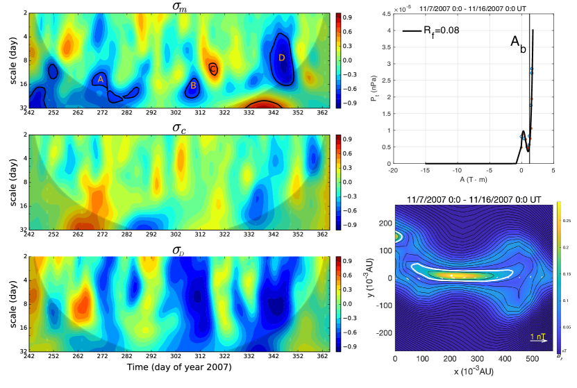
Zhao et al. (2019b) also identified magnetic flux rope or magnetic island structures behind the HTS.
These structures are identified as patches with enhanced magnetic helicity (), labeled as A–D in the top panel of Fig. 17. Since the feature of enhanced magnetic helicity is shared with circularly polarized Alfvén waves, a small cross helicity () and negative residual energy () are required for identifying magnetic flux ropes confidently.
The Grad–Shafranov (GS) reconstruction technique further confirms the finding by providing a reconstructed 2D cross section for one of the flux ropes as an example (bottom left panel).
The bottom right panel shows the curve from the GS reconstruction, where is the total pressure
and is the magnetic flux function. The double-folding pattern with a fitting residual of indicates a good fit quality.
The flux rope appears to have a scale size of AU.
The origin of flux ropes is unknown. In the supersonic SW small-scale magnetic flux ropes are often recognized as a representation of quasi-2D turbulence that is a majority component of the SW turbulence in this region (e.g., Zank et al., 2017a).
The flux ropes identified in the IHS may be evidence for 2D fluctuations in the outer heliosphere as they are transmitted and amplified downstream of the HTS. The compression at the HTS may also lead to enhanced magnetic reconnection, which generates multiple magnetic flux ropes.
Zank et al. (2018) described the transmission of MHD turbulence across the PUI-modified HTS using the NI MHD model. On the shock passage, the model predicts a strong amplification of the 2D component of turbulence, consistent with observations of flux ropes. The model also predicts a downstream state in which the turbulent kinetic energy dominates over the magnetic energy. However, the observed increase of magnetic turbulence variance is larger than predicted, which is possibly due to the presence of compressive modes not accounted for in Zank et al. (2018).
Zank et al. (2021) have recently analyzed in detail the transmission of 2D MHD modes (including acoustic, entropy, vortical, and magnetic island modes) across collisionless shocks. The agreement with V2 observations presented above suggest that these structures are an important component of MHD turbulence at the HTS.
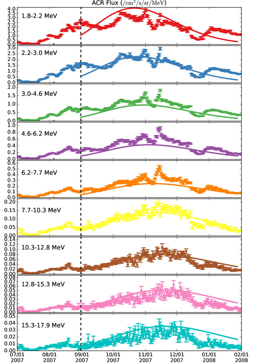
It has been suggested that magnetic flux ropes generated by magnetic reconnection may accelerate particles in a stochastic fashion, which may be partially responsible for the generation of anomalous cosmic rays in the inner heliosheath (Drake et al., 2010, 2017; Zank et al., 2015; le Roux et al., 2016). The idea is that enhanced magnetic reconnection in the IHS due to the compression associated with crossing the HTS leads to the generation of multiple magnetic flux ropes. The interaction between flux ropes then leads to particle acceleration. Zank et al. (2014b) presented a theoretical framework describing the acceleration and transport of particles in regions of interacting magnetic flux ropes, taking into account processes of magnetic island contraction and merging. The theory was applied by Zhao et al. (2018, 2019a) to an energetic particle event observed by Ulysses near 5 AU. In the event, the energetic particle fluxes are found to be strongly enhanced after the crossing of an interplanetary shock and the peak enhancement occurs 5 days after the shock crossing.
The Zank et al. theory was also applied to the ACR proton flux enhancement behind the HTS by Zhao et al. (2019b). Fig. 17 presents evidence of magnetic flux ropes after the HTS crossing, obtained from V2 LECP data. In Fig. 18, the ACR fluxes are shown for different energy channels between 1.8 MeV and 17.9 MeV. The measurements are fitted quantitatively to the Zank et al. (2014b) theory using a Monte Carlo Markov Chain (MCMC) technique, as shown by the solid lines in the figure. The fitted lines successfully reproduce that (i) there is enhancement of the ACR flux behind the HTS; (ii) the enhancement is stronger for higher energy particles within the considered energy channels; and (iii) the location of peak flux enhancement is further away from the shock for higher energy particles. We note that the analysis here applies only to the region very close to the HTS (within AU). It is likely that other acceleration mechanisms such as the diffusive shock acceleration are active deeper in the heliosheath. For recent reviews on ACRs and particle acceleration processes at collisionless shocks, see Giacalone et al. (2022) and Perri et al. (2022) in this volume.
5 Turbulence in the inner heliosheath
In the IHS the solar wind plasma is subsonic, having been decelerated at the HTS. Much of our current knowledge of turbulence in the IHS has been acquired via in situ (Voyager) observations. In particular, analyses of Voyager measurements suggest that significant levels of compressible fluctuations are present in the IHS (Burlaga et al., 2006a, 2008; Fisk and Gloeckler, 2008; Burlaga and Ness, 2009, 2012, 2012; Burlaga et al., 2014; Richardson and Burlaga, 2013; Fraternale, 2017; Fraternale et al., 2019a). Thus, the nature of the turbulence there differs from that in the supersonic SW upstream of the termination shock, where the fluctuations are predominantly incompressible (e.g., Tu and Marsch, 1994; Roberts et al., 2018).
Unfortunately, this compressible turbulence in the IHS is still poorly understood, from both the observational and the theoretical perspectives. Observationally, this is mainly due to the well-known limits of 1D measurements, unavailability of PUI measurements and plasma data (V1), and the level of noise. Consequently, to date, the dissipation regime of turbulence has been inaccessible to our investigations. On the theory side, compressible MHD turbulence is clearly richer than its incompressible counterpart having additional parameters such as the sonic Mach number and the plasma beta, . Aspects that can play important roles include the sub or supersonic character of the system, the size of the relative to unity, and the nature of any driving of the velocity field (e.g., is it the solenoidal velocity that is driven, the compressive component, or a combination). Simulation studies investigating various features of compressible MHD, such as energy transfer (both across scales and between magnetic, internal energy, incompressible , and compressive components), and variance and spectral anisotropy have been reported on and these may provide starting points for understanding IHS Voyager observations (e.g., Ghosh and Matthaeus, 1990; Cho and Lazarian, 2002, 2003; Vestuto et al., 2003; Carbone et al., 2009; Kowal and Lazarian, 2010; Banerjee and Galtier, 2013; Oughton et al., 2016; Grete et al., 2017; Hadid et al., 2017; Yang et al., 2021). However, further studies are surely needed, including ones tailored to IHS conditions.
5.1 An overview of the observed structures in the IHS
In general, turbulence is present in the IHS and consists of both random fluctuations and coherent structures. The HTS is certainly the major source of turbulence in the IHS, at least in the direction of the heliospheric “nose”, as it transmits and possibly amplifies the full spectrum of fluctuations from the supersonic SW to the IHS (e.g., Zank et al., 2018, 2021).
5.1.1 Large-scale fluctuations
On large scales, transient structures of solar origin such as global merged interaction regions (GMIRs) have been observed in the IHS (Burlaga et al., 2011, 2016; Richardson et al., 2017). They are associated with strong magnetic fields and enhancements of plasma density and temperature, and may be moving fast enough to generate shocks or pressure pulses. When GMIRs interact with the HP, they produce transmitted shocks or compression waves in the VLISM, and reflected perturbations in the IHS. Figure 19 from Borovikov et al. (2011) shows an example of the complex patterns and the different fluctuation modes that can arise as a consequence of corotating streams interacting with the HTS. Time dependent and data-driven 3D simulations are necessary to understand the dynamics and time-space evolution of the large-scale structures in the outer heliosphere. A recent study by Pogorelov et al. (2021), provides animations of magnetic and thermal pressure along V1 and V2 trajectories from earlier numerical solutions of Pogorelov et al. (2017b); Kim et al. (2017b). Large-scale features include the sector structure, however it is well known that the periodic sector structure no longer exists beyond AU (e.g., Burlaga, 1994; Pogorelov et al., 2017a). In fact, in the IHS, sectors and regions with mixed polarity show complicated polarity patterns. V1 and V2 have observed regions of mostly unipolar fields and “sector regions” of mixed polarity, statistically characterized by Richardson et al. (2016). The sector region is the region swept by the HCS. The presence of two topologically different regions within the IHS suggests that the properties of turbulence should also change across these regions, with implications for the transport of energetic particles (Burlaga et al., 2009; Opher et al., 2011; Florinski et al., 2013b; Hill et al., 2014). The properties of turbulence in the heliotail are unknown and will not be discussed here. Numerical models show the strong, likely dominant effect of the solar cycle variations on the generation of large-scale structures in the tail (Pogorelov et al., 2017a) and the possible onset of large scale instabilities of various nature of the collimated SW lobes at high latitudes, a prominent feature of steady-state, spherically-symmetric solutions (Yu, 1974; Pogorelov et al., 2015; Opher et al., 2021).
Besides the structures of solar nature, instabilities at the HP may also play an important role in the injection of fluctuation energy in the heliosheath at large scales ( AU) and the generation of structures in the IHS. Long before V1 actually observed signatures of HP instability (Burlaga et al., 2013b, August 2012, DOY 210 – 238), Fahr et al. (1986) first suggested that the HP may undergo Kelvin–Helmholtz (KH) instability at the HP flanks, and may also be Rayleigh–Taylor (RT) unstable due to local accelerations of the HP, especially when the HMF is weak. Early studies on this topic were conducted by Baranov et al. (1992); Chalov (1994, 1996); Liewer et al. (1996); Zank et al. (1996b); Belov and Myasnikov (1999); Zank (1999a); Pogorelov (2000); Ruderman (2000); Florinski et al. (2005); Ruderman, M. S. and Brevdo, L. (2006); Borovikov et al. (2008). In particular, Liewer et al. (1996) and Zank et al. (1996a) highlighted the role of the ion-neutral drag on the possible development of RT near the nose. Zank (1999a) have shown that charge exchange between neutrals and ions acts essentially as an effective gravitational term that can trigger the RT instability. Borovikov et al. (2008) further identified a mixed RT–KH form of instability on the HP flanks, assisted by hot secondary neutrals created by charge exchange in the SW. As shown by Borovikov et al. (2008) the absence of HMF can increase the instability dramatically. Borovikov and Pogorelov (2014) simulated a 3D heliosphere and demonstrated that the RT instability is considerably suppressed near the HP nose by the unipolar, unrealistically large, HMF in steady-state models, but is triggered in the presence of solar cycle effects. This is why accounting for solar cycle in simulations is not important per se, but because it creates favorable conditions for the instability to develop, when is small due to the presence of sector regions (see also Pogorelov et al., 2021). Analytic studies of the RT instability have also been carried out (Avinash et al., 2014; Ruderman, 2015). Results in Pogorelov et al. (2015) indicate that only the KH instability is found in the tail region. Eventually, solar cycle simulations of Pogorelov et al. (2017b) suggested that at the time of the HP crossing the KH/RT instability was more likely to occur at northern latitudes, while magnetic reconnection may reveal itself as a tearing mode (plasmoid) instability at southern latitudes (see Fig. 31). A situation similar to the RT instability is found in the magnetic flux tube interchange instability, proposed by Krimigis et al. (2013) to explain V1 observations and investigated theoretically by Florinski (2015). This instability may develop on smaller scales (–5 AU), and results from the positive plasma pressure gradient and the IMF curvature.
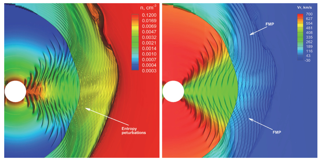
5.1.2 Fine-scale fluctuations
Ion-scale coherent features observed in situ in the IHS include current sheets (CS) described by Burlaga and Ness (2009, 2011) as proton boundary layers, magnetic holes, and magnetic humps. Their typical size lies in the range of –30 , where is the proton cyclotron radius of the plasma mixture ( K). The exact nature of these structure is unknown, but an hypothesis was advanced by Burlaga and Ness (2009) that they originate from mirror mode instability and evolve nonlinearly as solitons, and eventually as pressure balanced structures. A theory of solitary waves has been proposed by Avinash and Zank (2007). Mirror mode instabilities have been identified near the HTS (Liu et al., 2007; Génot, 2008; Fahr and Siewert, 2007) and within the IHS by Tsurutani et al. (2011a) and Tsurutani et al. (2011b), who also pointed out the role of PUIs in the amplification of this instability.
As discussed in Sec. 3, models aiming at a quantitative treatment of turbulence in the entire inner heliosheath are sparse. One of the first was presented by Usmanov et al. (2016) who used a four-fluid model to simulate the heliosphere and nearby LISM, including the transport of turbulence in this whole region. The turbulence is modeled using a one-component model for incompressible MHD turbulence, and thus, as the authors explicitly state, cannot address the presence or role of compressive fluctuations. Nonetheless, the work demonstrates the principal feasibility of such extensions of previous inside-the-HTS transport modeling to regions beyond the HTS. Despite its limitations the model provides a valuable reference case for forthcoming simulations. A second model by Fichtner et al. (2020) has recently addressed the problem of generating compressible fluctuations throughout the whole IHS. It applied the quasilinear theory to the initial evolution of compressible wave modes using initial values obtained from a simulation of a 3D model of the SW/LISM interaction. The basic idea is that the compressible fluctuations are a result of the proton mirror instability, which is a consequence of a perpendicular temperature anisotropy (with referring to the orientation relative to the local magnetic field direction ). The resulting fluctuations in proton number density are anticorrelated with the associated magnetic fluctuations via the relation (e.g., Liu et al., 2007)
| (19) |
To compute these fluctuations throughout the IHS the structure of the latter was determined from a numerical simulation of the 3D large-scale heliosphere using the MHD code Cronos (Kissmann et al., 2018) for the model equations formulated in Wiengarten et al. (2015). These equations are the usual MHD equations for the large-scale quantities and Eqs. 13 to 15 with the simplifying assumptions , , and the choice . Using the solutions of this model obtained for the IHS Fichtner et al. (2020) applied the theory of temperature anisotropy-driven kinetic instabilities reviewed by Yoon (2017).
The central results are summarized with Fig. 20.
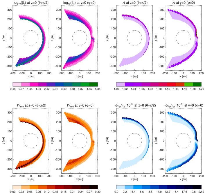
The upper right panel reveals that the quasilinear evolution results in anisotropy values (that were initially ) a little above unity across most of the IHS, which is consistent with the findings by, e.g., Liu et al. (2007) and Fahr and Siewert (2007). The corresponding magnetic energy density of the mirror mode-induced compressive fluctuations (lower left panel) and, via Eq. (19), the associated, locally generated density fluctuations (lower right panel) are significant in large regions of the IHS, particularly also below a latitude of about , i.e., in the region probed by the Voyager spacecraft. At high northern latitudes and within the equatorial plane, the energy density is decreasing towards the heliopause, which appears to reflect the distribution of the plasma beta. A comparison of the magnetic energy density associated with the mirror-mode instability with that associated with the MHD fluctuations as obtained from the Cronos simulation revealed that the compressible fluctuations indeed dominate in most parts of the inner heliosheath: only in the equatorial and high-latitude downstream vicinities to the termination shock do the incompressible fluctuations prevail.
The computed the energy density of the locally generated magnetic fluctuations and the associated density fluctuations may serve as source terms in forthcoming models of the actual turbulence transport in the IHS.
5.2 A statistical description of IHS fluctuations
The description of turbulence obviously also requires a statistical approach. A series of studies (Burlaga, 1991; Burlaga et al., 2003a; Burlaga, 2004; Burlaga et al., 2006b; Burlaga and Ness, 2010; Macek et al., 2012; Macek and Wawrzaszek, 2013; Burlaga et al., 2013b; Macek et al., 2014) demonstrated the existence of a multifractal scaling symmetry for large-scale fluctuations ( day) in the distant SW and IHS. The multifractal formalism is a powerful classical tool to describe the structure of the dissipation rate in turbulence (see, e.g., Meneveau and Sreenivasan, 1987; Frisch, 1995). The analysis of the fluctuations of led to remarkable outcomes, such as demonstrations of (i) the existence of a power spectral regime on scales in the range of 1–100 days (e.g, Burlaga and Ness, 2013) and (ii) the presence of large-scale intermittency, although at lower levels with respect to the supersonic SW (see Richardson et al., 2022). Burlaga and Ness (2013) applied the “-triplet” concept from the nonextensive statistical mechanics (Tsallis, 2009) to provide evidence that fluctuations in the IHS are in a quasi-stationary, metaequilibrium state. Other studies (Burlaga and Ness, 2009; Burlaga et al., 2013b, 2019b) indicate that magnetic field increments for time lags from 48 s to 1 day are well described by the -Gaussian distribution with parameters , , :
| (20) |
with the parameter is related to the kurtosis (or flatness) and is found to be as large as 1.6 in the IHS ( corresponds to Gaussian statistics). Burlaga et al. (2009, 2010, 2017) have also shown that the daily distributions of are typically log-normal in the sector regions, but Gaussian in unipolar regions.
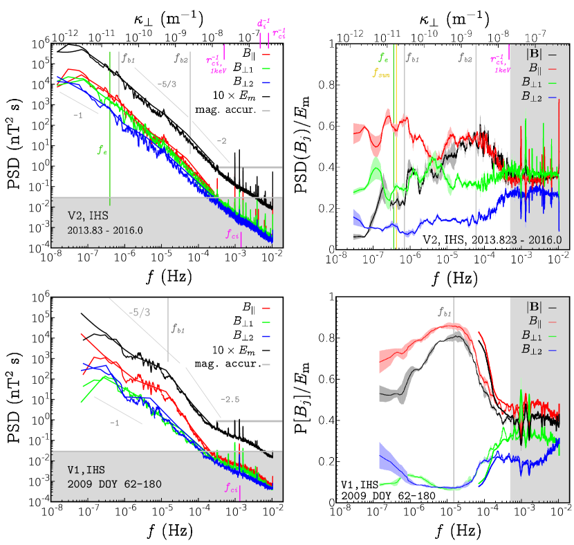
The presence of intermittency and scaling laws are key ingredients of turbulence. To the best of our knowledge, evidence for the existence of different power-law regimes throughout the IHS was provided for the first time by Fraternale (2017) and Fraternale et al. (2019a, b). They conducted a spectral analysis of V1 and V2 high-resolution (48 s) magnetic field data in several sector and unipolar regions identified by Richardson et al. (2016) and Burlaga et al. (2017). Results are set forth in terms of power spectra and structure functions up to the fourth order. Such analysis is challenging because of the sparsity of the 48 s data. After the HTS, about 70% of data points are missing due to tracking issues, noise, instrumental interference, and other reasons. Therefore, the combined use of different spectral estimation techniques becomes mandatory to rule out the numerous artifacts in the statistics. In particular, compressed sensing, a recent paradigm in signal processing (Donoho, 2006; Candes et al., 2006a, b), was successfully applied to SW turbulence analysis for the first time by Gallana et al. (2016) and Fraternale (2017), and subsequently applied to the analysis of IHS and VLISM Voyager data, and magnetospheric turbulence (Sorriso-Valvo et al., 2019).
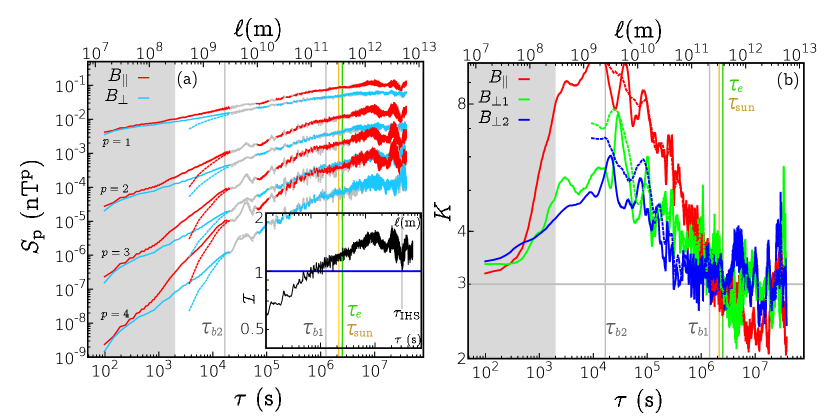
Figure 21 shows two examples of magnetic field turbulence spectra computed using 2 years of V2 observations in a sector region at AU (top panels) and 120 days of V1 data at AU (bottom panels). The PSD is shown in the left panels, while the right panels show the scale-dependent variance anisotropy and the magnetic compressibility. The Larmor radius of thermal protons, km, the ion inertial length km, and the Larmor radius of 1 keV PUIs ( km) are shown in the top panels. The Taylor (frozen flow) hypothesis is applied only at V2, to obtain a rough estimate of the wavenumber perpendicular to , under the assumption of wavenumber anisotropy, . Clearly, 1D spectra contain contributions from all wave vectors. However, as pointed out by Fraternale et al. (2019a) and Zieger et al. (2020), its application in the IHS is more critical than in the supersonic SW. The main reasons for this are the lower bulk flow speed ( km s-1 at V2), the presence of shocks and, possibly, finite-amplitude fluctuations of dispersive nature, whose propagation speed is affected by the energetically dominant population of PUIs.
At the large scales, Fraternale (2017) and Fraternale et al. (2019a) confirmed the existence of a spectral regime in the frequency spectrum, which is typically observed for Hz. They discussed the extension of this regime in the frequency space. A new finding was that a spectral break (labeled as in Fig. 21) separates the regime from other power-law regimes observed at smaller scales. The regime may be considered as a reservoir of energy for the turbulent cascade. Its frequency span was found to decrease with distance and to be larger in unipolar regions than in sector regions. In the example of Figs. 21(top) and 22, the spectral break is seen at Hz ( AU). There is a possibility that the regime originates from SW turbulence being processed by the HTS (see also Fig. 16). It may include perturbations such as those shown in Fig. 19 and all large-scale structures described previously, but its nature remains unclear.
At higher frequencies ( Hz) an inertial cascade regime was identified. In the unipolar regions sampled by V1, the (absolute) spectral index becomes large, , which is mainly ascribed to the dominant component. At V2, a second spectral knee (, in the figures) is observed at Hz ( AU, ). This separates a Kolmogorov-like regime where from a steeper, power-law regime where . A remarkable finding is that both the magnetic compressibility (black curves in the right panels of Fig. 21) and the intermittency (Fig. 22) reach a maximum at this scale. Fraternale et al. (2019a) and Fraternale et al. (2019b) have suggested the possibility that the spectral steepening may be ascribed to PUI-scale kinetic processes, even though these studies did not provide a model. In compressible turbulence, the presence of a variety of compressible and incompressible coherent structures, dispersive waves (e.g., Perrone et al., 2016) and magnetic reconnection (Loureiro and Boldyrev, 2017) may all contribute to an increased turbulence cascade rate at scales smaller than the typical size of CSs, . Although the gyroscale of thermal protons lies in the last frequency decade in Voyager measurements, PUI-related effects might be observed at smaller frequencies near Hz. The spectral knee may then be ascribed to the typical size (passing times, at Voyager) of the kinetic structures described previously in this section (Burlaga et al., 2006a). This may represent a “transition scale” from the MHD to the kinetic regime of turbulence, similar to what was observed (e.g., Alexandrova et al., 2008) near the ion scale in the supersonic SW. However, here the transition would occur between the PUI gyroscale and the thermal ion scale. The reduction of compressibility and intermittency at higher frequencies is also a known feature in the SW near 1 AU, ascribed to kinetic wave activity (e.g., Kiyani et al., 2009; Wu et al., 2013; Alexandrova et al., 2013; Sorriso-Valvo et al., 2017; Bale et al., 2019). Here, it may be related to PUI kinetic activity but it may also be an artifact of noise in the measurements, and deserves further investigations.
At finer scales in the range Hz, all spectra flatten significantly. Certainly, this regime is affected by the presence of noise in the measurements ( errors are in the range of 0.02–0.05 nT, Berdichevsky, 2009), including the noise from the fluxgate magnetometers (Behannon et al., 1977). It should also be noted that the spikes at harmonics of Hz are certainly instrumental artifacts. Some spectral techniques may make them appear broader then they are. Interestingly, during some intervals, a further spectral steepening can be observed near the cyclotron frequency of the thermal plasma ( Hz). A clear example is provided in the bottom panels of Fig. 21 for V1 data in 2009. Using multi-ion fluid simulations, Zieger et al. (2020) suggested that fast-mode turbulence originating from nonlinearly steepened fast-magnetosonic waves may explain V2 observations in the high-frequency regime near the HTS. Further investigations are needed to understand which processes dominate the transitional and the dissipation regimes of turbulence in the IHS. Gutynska et al. (2010) observed a damping of higher frequencies with distance, which supports the idea that fluctuations are generated and/or amplified at the HTS. However, the persistence of large magnetic compressibility deeper in the IHS, as shown in Fig. 21, poses a number of questions about the physical processes responsible for the production of high-frequency fluctuations and the turbulent energy transfer across scales.
Second order statistics (i.e. PSDs) are not sufficient to assess the presence of turbulence. The evidence of turbulence in the IHS is supported by the existence of clearly defined power-law regimes in higher order statistics such as the structure functions, . An example is provided in the left panel of Fig. 22 for V2 data in a sector region. Fraternale et al. (2019b) also shown that the extended self-similarity principle (Benzi et al., 1993) can be successfully used to obtain the SF relative scaling exponents from Voyager data. The black curve in the insert shows that at V2 the low-frequency spectral break occurs when the condition is met. As described by Matteini et al. (2018) in the case of supersonic SW turbulence, the “saturation” of the turbulent cascade at is the result of incompressible fluctuations being bounded on a sphere of radius equal to , which introduces another scale in the system. This condition is not reached in unipolar regions at V1, where the maximum intensity is about 0.7 in the energy injection regime.
The above observations are suggestive of the presence of a highly structured, anisotropic magnetic turbulence cascade in the IHS, but are far from being conclusive on the nature of turbulence in this region. What happens in the transitional regime near the ion scale and at sub-ion scales is a topic of particular interest in theoretical analysis (e.g., Chen and Boldyrev, 2017; Chen et al., 2020; Bowen et al., 2020a, b). Further analyses of compressible, IHS turbulence are necessary to improve our theoretical understanding of MHD turbulence and its impact on the global shape of the heliosphere.
6 Turbulence in the very local interstellar medium
The interstellar medium has been long recognized to be turbulent on scales up to pc (Lee and Jokipii, 1976; Armstrong et al., 1981). A signature of turbulence is the impressive power-law spectrum of density fluctuations (dubbed “The Big Power Law”) obtained by Armstrong et al. (1995) and extended later by Chepurnov and Lazarian (2010) (see Fig. 23). The density spectral index is between and , which is consistent with the presence of Kolmogorov-like turbulence on scales from m to m, but does not exclude the presence of shock-like structures. Such insights on the ISM irregularities have been obtained via remote observations, such as radio scattering and scintillations, dispersion measures, Faraday rotation measures, spectroscopy, etc. In the ISM, energy is injected over a wide range of scales from different processes, and turbulence is certainly not statistically homogeneous, as discussed in the extensively by Ferrière (2001), Elmegreen and Scalo (2004), Scalo and Elmegreen (2004), see also Redfield and Linsky (2004). Recent findings on inhomogeneities in the Local Interstellar Cloud (LIC) in which the heliosphere is immersed, are discussed by Linsky et al. (2022) in this volume.
The LISM properties are affected by the presence of the heliosphere over distances of the order of several hundred AU (Holzer, 1989; Zank, 2015), or exceeding AU, from the perspective of TeV GCRs (Zhang et al., 2020). It is reasonable to believe that the properties of interstellar turbulence may change with the distance from the HP. Therefore, is should be clarified that the in situ observations are likely not representative of the entire VLISM, but of a narrow, very dynamic region near the HP.
The first in situ observations of interstellar turbulence have been made after the crossing of the heliopause (HP) by the V1 spacecraft in 2012 August (122 AU) and by V2 in 2018 November (119 AU) (e.g., Stone et al., 2013; Burlaga et al., 2019a). A currently accepted hypothesis is that turbulence in this region consists of a superposition of the unperturbed LISM turbulence and fluctuations induced by heliospheric processes on scales ranging from the year solar cycle to plasma kinetic scales (Burlaga et al., 2015, 2018; Zank et al., 2017b; Fraternale et al., 2019a; Matsukiyo et al., 2019; Lee and Lee, 2019, 2020; Fraternale and Pogorelov, 2021).
Major shock/compression waves have been observed at V1 (Burlaga et al., 2013a; Burlaga and Ness, 2016; Burlaga et al., 2017, 2021). They are transmitted into the VLISM when SW perturbations such as GMIRs hit the HP on the inner side, as was first suggested by Gurnett et al. (1993) and later demonstrated in several simulations (Steinolfson et al., 1994; Pogorelov, 1995, 2000; Zank and Müller, 2003; Washimi et al., 2011; Borovikov et al., 2012; Pogorelov et al., 2013b; Fermo et al., 2015; Kim et al., 2017b). Compressible, finite-amplitude waves may undergo nonlinear steepening and interactions and can occasionally merge to produce larger waves (e.g., Pogorelov et al., 2021). These shock-like perturbations are associated with plasma wave events and 2–3 kHz radio emissions first detected at 1 AU by Kurth et al. (1984); Gurnett et al. (1993) and recently observed in situ by Voyager’s Plasma Wave Subsystem (PWS) (Gurnett et al., 2015; Gurnett and Kurth, 2019; Kurth and Gurnett, 2020). It is believed that radio emissions can be excited by interstellar shocks provided that primed nonthermal electrons exist in that region. In fact, electrons can be primed via resonant acceleration by a lower hybrid wave (LHW) mechanism which, in turn, may be driven by instabilities of ring-beam PUI distributions (Omelchenko et al., 1989; Cairns and Zank, 2002). In addition, shocks and compression waves may induce the observed anisotropy of GCR proton fluxes (Gurnett et al., 2015; Rankin et al., 2019). Details are discussed in Mostafavi et al. (2022) and Richardson et al. (2022) in this volume.
An important contribution to building a theory of interstellar (Alfvénic) turbulence was given by Sridhar and Goldreich (1994); Goldreich and Sridhar (1995). A model of VLISM turbulence has not been developed yet. A number of physical processes and factors should be considered to understand and model turbulence and dissipation in the VLISM. These include:
-
1.
Motion of the HP, i.e. the “forcing effect” associated with the solar activity and HP instabilities;
-
2.
Bow wave/shock effect on the VLISM turbulence;
-
3.
Shock/turbulence interactions, at MHD and kinetic scales;
-
4.
Coulomb collisions;
-
5.
Charge exchange collisions, kinetic instabilities due to the presence of supra-thermal particles;
-
6.
GCR/turbulence interaction;
-
7.
Partial ionization of the medium;
6.1 In situ observations of magnetic field turbulence in the VLISM
Burlaga et al. (2015) presented the first in situ observations of magnetic turbulence in the VLISM from V1 MAG data at the 1 day resolution. (Burlaga et al., 2015) and Burlaga et al. (2018) investigated two relatively “quiet” intervals between shocks at a distance of AU and AU, respectively. It was shown that (i) the intensity of turbulence is low, , which is close to the estimated level of systematic uncertainties ( nT or larger for the component) and to the magnetometer’s limit (Burlaga and Ness, 2014a). (ii) the trace power spectra exhibit a power law with a Kolmogorov-like spectral index; (iii) on relatively large scales (–100 days), the fluctuations were highly compressive in the 2013–2014 interval, closer to the HP, but (iv) the compressibility decreased in 2015–2016, which suggested an evolution toward an Alfvénic state with distance.
It should be noticed that the terminology “weak” is often used improperly to indicate a low intensity of local fluctuations with respect to the average field. This condition is satisfied in the weak (wave) turbulence phenomenology (e.g., Zakharov et al., 1992; Galtier et al., 2000; Schekochihin et al., 2012), but is not sufficient. The strength of nonlinear interactions must also be evaluated (see discussion in, e.g., Oughton and Matthaeus, 2020), as well as the kind of turbulence forcing. So far, this investigation has not been possible from Voyager data in the VLISM. To date, detecting weak turbulence regimes in the VLISM turbulence remains an open challenge.
Another open science question concerns the properties of the unperturbed LISM turbulence. Burlaga et al. (2015) considered the possibility that in the 2013 quiet interval turbulence was not much affected by the solar activity, and extrapolated the Kolmogorov spectrum to reach the saturation condition , assuming nT. Updated results presented by Burlaga et al. (2018), show that the outer scale obtained from the extrapolation is pc. It was suggested that this scale may be interpreted as the outer scale of turbulence in the VLISM.
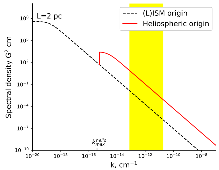
Some recent studies suggested that the observed turbulence is indeed affected by the presence of the heliosphere, as far as 25 AU from the HP. In particular, Zank et al. (2017b) analyzed theoretically the “radiation” of small-amplitude waves by the HP into the VLISM. They have shown that IHS fast- and slow-mode waves incident on the HP generate only fast-mode waves that propagate into the VLISM. This result was confirmed by hybrid simulations of Matsukiyo et al. (2019), and provides a plausible explanation for the observed large values of compressibility of VLISM turbulence observed by Burlaga et al. (2015). Figure 24 from Zank et al. (2019) illustrates a possible scenario where the transmitted spectrum is superimposed on a Kolmogorov-type model spectrum (Giacalone and Jokipii, 1999) of LISM turbulence, that would have an outer scale of 2 pc. Notice that this scale is smaller than the largest ISM scales shown in Fig. 23, but may be consistent with the size of the LIC . Interestingly, the recent investigations of the LIC properties reviewed by Linsky et al. (2022) reveal the presence of temperature inhomogeneities in the LIC on scales smaller than 4,000 AU. According to the scenario depicted in Fig. 24, the outer scale of the locally transmitted turbulence may be of the order of AU, compatible with frequencies of the order of the solar cycle.
Fraternale et al. (2019a) analyzed four V1 intervals out to 135 AU, including two new periods in post-shock, “disturbed”, regions. They used 48 s resolution data and were able to detect the presence of intermittency in the frequency range Hz, which is mostly observed in the transverse components of . Spectral indices, structure function exponents, and the turbulence intensity for the parallel and perpendicular components are summarized in Table 5 of Fraternale et al. (2019a). It was noted that a common feature of all periods is the high magnetic compressibility in the high frequency regime. For instance, see panel (d) in Fig. 27. This is relevant because (i) it may indicate that physically relevant information may be obtained using high resolution Voyager data, despite the high level of noise, and (ii) new questions arise about the turbulent injection and dissipation of fine scale compressible modes. It was also suggested that interstellar shocks might affect the properties of turbulence.
Zank et al. (2019) investigated theoretically the nonlinear interaction of linear wave modes in the VLISM, in the NI MHD framework. In particular, two cases were considered. The first case is that a fast-mode wave with a 2D, zero-frequency mode to generate a slow-mode wave. In this scenario, the wavenumber of the latter mode would be larger by a factor . The second case is that a fast mode wave plus a zero-frequency mode generates an Alfvén mode with similar wavenumber. Here, the predominantly fast-mode spectrum transmitted at the HP would be replaced by an Alfvén-mode spectrum within a certain distance from the HP, estimated to be AU by Zank et al. (2019). Both mechanisms may play a role in the VLISM.
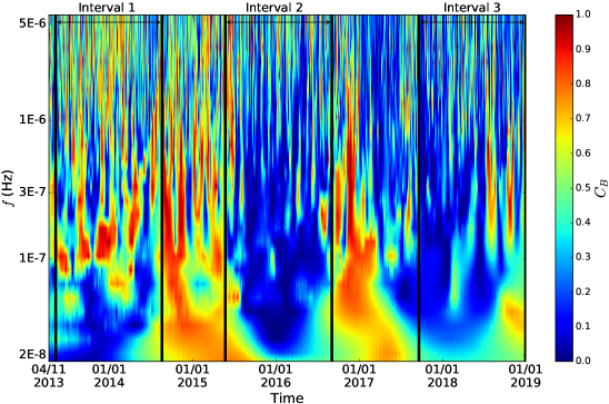
Fraternale et al. (2020) provided the first evidence of fine-scale intermittent turbulence with in the precursor of the shock wave that crossed V1 on day 236 of 2014. In this case, the frequency range of scales of interest is Hz (, where km was estimated using K). The turbulent cascade exhibits coherent fine-scale structures compatible with a filamentary topology, and an unexpectedly steep spectrum for the transverse fluctuations. A relevant implication of this study is that the HBL is not featureless on scales smaller the thermal proton-proton Coulomb collisional mean free path ( AU for –30,000 K). Moreover, a question is raised about if the weak subcritical shocks in the VLISM are capable of accelerating ions in their foreshock. A detailed discussion of this specific turbulence event is presented in Sec. 4.4 of Mostafavi et al. (2022) in this volume. Here, the trace PSD is shown in panel (d) of Fig. 27.
Zhao et al. (2020) performed a wavelet and Hilbert spectral analysis of three “quiet” periods using daily data, focusing on the evolution of the magnetic compressibility. Figure 25 from that study shows the wavelet spectrogram of the magnetic field strength, normalized by the trace spectrogram. Zhao et al. (2020) concluded that a conversion from compressible to incompressible turbulence occurs within the first interval, in particular the compressive fluctuations are confined within a spatial region of AU from the HP. This seems in agreement with Zank et al. (2019) for wavenumbers in the range . Such a decrease of compressibility with distance was also addressed by Burlaga et al. (2020b). However, some questions are still open regarding this point. Fraternale and Pogorelov (2021) pointed out that the decrease of compressibility with distance is not smooth, and is largely due to an increase of , rather than a decrease of . During 2018–2019, the level of compressibility was larger than during 2015–2016 due to the presence of compressible waveforms with similar amplitude and periodicity of those observed in 2013–2014 (see Fig. 26). Compressible wave-like structures have been observed by V1 during 2021 out to 150 AU from the Sun (Burlaga et al., 2021). The data analyses of post-shock intervals by both Fraternale et al. (2019b) and Zhao et al. (2020) suggest that time dependent effects and shock-wave interactions may both affect Voyager observations, in addition to the mode conversion processes described by Zank et al. (2019). Data-driven, global simulations of Kim et al. (2017b) have shown that the largest compressible perturbations can reach far distances, beyond 200 AU. An interesting aspect not yet fully understood is the scale-dependent evolution of the magnetic compressibility. In fact, is found to grow with the frequency, reaching a maximum of in the high-frequency regime near MHD/ion-kinetic transitional scales (see Fig. 27(c)), which is unlikely to be an artifact of noise.
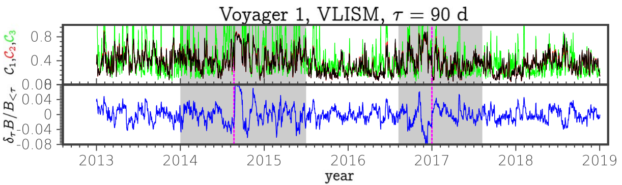
Lee and Lee (2020) and Fraternale and Pogorelov (2021) performed a detailed spectral analysis of magnetic turbulence observed by V1 until 2019. They described the fluctuations in the frequency range Hz ( m-1) using 48 s data at V1, providing further evidence of the heliospheric influence on the observed VLISM turbulence out to 150 AU. Examples of magnetic energy spectra are shown in Fig. 27. Characteristic scales of the thermal plasma and energetic particles are reported in panel (a), including also the proton and electron GCR gyroscales obtained by Rankin et al. (2020). Lee and Lee (2020) also performed a combined analysis of magnetic field and plasma wave data and analyzed short time intervals in the wavenumber range m-1. By comparing observations and the theoretical dispersion relations of MHD modes, they concluded that at these scales no linear modes can explain Voyager observations, and turbulence might be associated with arc/spherically polarized Alfvén wave modes.
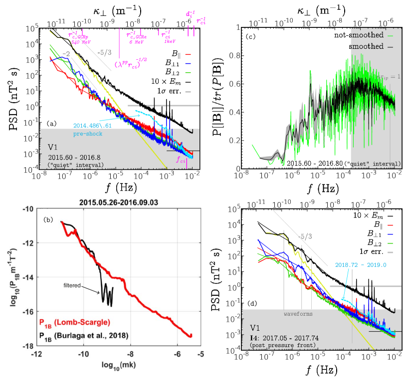
Fraternale and Pogorelov (2021) have shown that the spectrum of fluctuations on frequencies Hz is dominated by quasi-periodic waveforms with the period of 10–100 days (–2 AU). Such oscillations determine the breaks in multi-scale statistics. Often, they have a mixed compressive/transverse nature and display “N-wave” profiles that may be ascribed to nonlinear steepening (Whitham, 1974; Webb et al., 1993). Wave trains are particularly intense in post-shock intervals, as noted by Burlaga and Ness (2016); Burlaga et al. (2019b), and also by Burlaga et al. (2021). From an estimate of the turbulent Alfvén Mach number (–0.1), Fraternale and Pogorelov (2021) argued that such fluctuations may have been amplified locally due to the encounter with one or more shocks but their nature is still unclear. They estimated that the magnetic pressure fluctuations in quiet intervals, Pa, is a significant fraction (up to 50%) of the pressure jump associated with the shocks. In analogy with well known results of shock/turbulence interaction in fluids (e.g., Lele and Larsson, 2009) or collisionless plasmas (e.g., Trotta et al., 2021), this suggests that the structure and propagation of interstellar shocks/compression waves may be affected by turbulence (and viceversa).
Panels (a), (b), and (c) of Fig. 27 show results for the 2015.5–2016 quiet interval at V1. Panel (b) is taken from Lee and Lee (2020), and also shows the PSD obtained by Burlaga et al. (2018). Panel (d) shows spectra during 2017–2018. This interval follows a large pressure pulse that crossed V1 in 2017.0. At frequencies Hz (), a Kolmogorov-like spectral form is generally observed. However, Fraternale and Pogorelov (2021) pointed out that interpreting fluctuations as a classic Kolmogorov turbulence may be too simplistic a view, at least in the HBL. Both spectral index anisotropy and variance anisotropy are observed. Occasionally, the spectral index is close to -2, which may be partially ascribed to a coherent-cascade scenario, an example of which is the Burgers’ turbulence phenomenology. A common feature in all V1 intervals is the flattening at Hz. Certainly, the presence of noise in MAG data and the may affect this range of frequencies (Burlaga et al., 2014). Burlaga et al. (2018) applied a low-pass filter to exclude this range. Being aware of that, one can notice that significant anisotropy and variations of the power laws are observed in the high frequency MHD regime. Since these features are not typical of random noise, recent studies suggest that physically relevant fluctuations in the microscale regime (–1000 ) may be present in Voyager data. A striking example is the intense foreshock turbulence event (see the light-blue curve in Fig. 27(a)). A similar intensification of fine-scale turbulence was also observed in late 2018 (panel d). Therefore, a question arises regarding whether local mechanisms may be responsible for the injection of wave power in this regime.
A relevant physical aspect that may affect turbulence in the VLISM is the plasma collisionality with respect to Coulomb collisions. Recent estimates for the transport coefficients parameters can be found in Baranov and Ruderman (2013); Mostafavi and Zank (2018); Fraternale and Pogorelov (2021). The collisional transport theory holds if , and , where we indicate with () the fluctuation scale in the direction perpendicular (parallel) to , and with the proton–proton Coulomb collisional mean free path. Since V1 is likely sampling mostly , Fraternale and Pogorelov (2021) argued that part of observed fluctuations in the high frequency range of the spectrum do not satisfy the first condition. The cutoff perpendicular scale would be in the range of – AU for –30,000 K (–4 AU). This is reported in Fig. 27(a). According to Baranov and Ruderman (2013), the Reynolds number based on the bulk VLISM flow and a reference length of 100 AU is relatively low, , while the magnetic Reynolds number is . The later estimates of Fraternale and Pogorelov (2021) confirm the huge separation of viscous and resistive scales (large magnetic Prandtl number, ). These peculiar conditions have been investigated by means of numerical simulations of compressible turbulence by Cho and Lazarian (2002), and a model that was proposed by Cho et al. (2003) (see also Biskamp, 2003, and references therein). They found the existence of a viscosity-damped regime where magnetic field fluctuations follow a shallower, , spectral form at scales smaller than viscous cutoff, where the velocity field is smooth. Such spectral behavior resembles Batchelor’s (1959) viscous–convective subrange for a passive scalar in hydrodynamics. However, the magnetic field is dynamically important and the analogy with the passive scalar cascade may not always be appropriate. The relevance of these finding to the observed VLISM turbulence is the subject of current investigation. An estimate of the effective Reynolds number (Matthaeus et al., 2005) based on the observed correlation scale and the ion inertial length gives (Fraternale and Pogorelov, 2021).
Intermittency in the VLISM has been observed by Fraternale et al. (2019a), and a detailed investigation of quiet intervals was carried out by Burlaga et al. (2020a) using 1 h increments. They have shown that the intermittency in the transverse component is dominant in the VLISM beyond several AU from the HP. The kurtosis reaches values up to 7. Burlaga et al. (2020a, b) also provide the first observation of VLISM turbulence at V2. Here, intermittency is significantly larger than at V1, the compressible fluctuations are dominant at Hz and the intermittency is greater for the compressible component than for the transverse one, with kurtosis values exceeding 12. In the high-frequency regime, it is typically very difficult to observe intermittency due to noise in the measurements. We note that so far such observations have only been made in the regions of enhanced fluctuations described previously, and that the actual levels of intermittency may be higher than the observed ones.
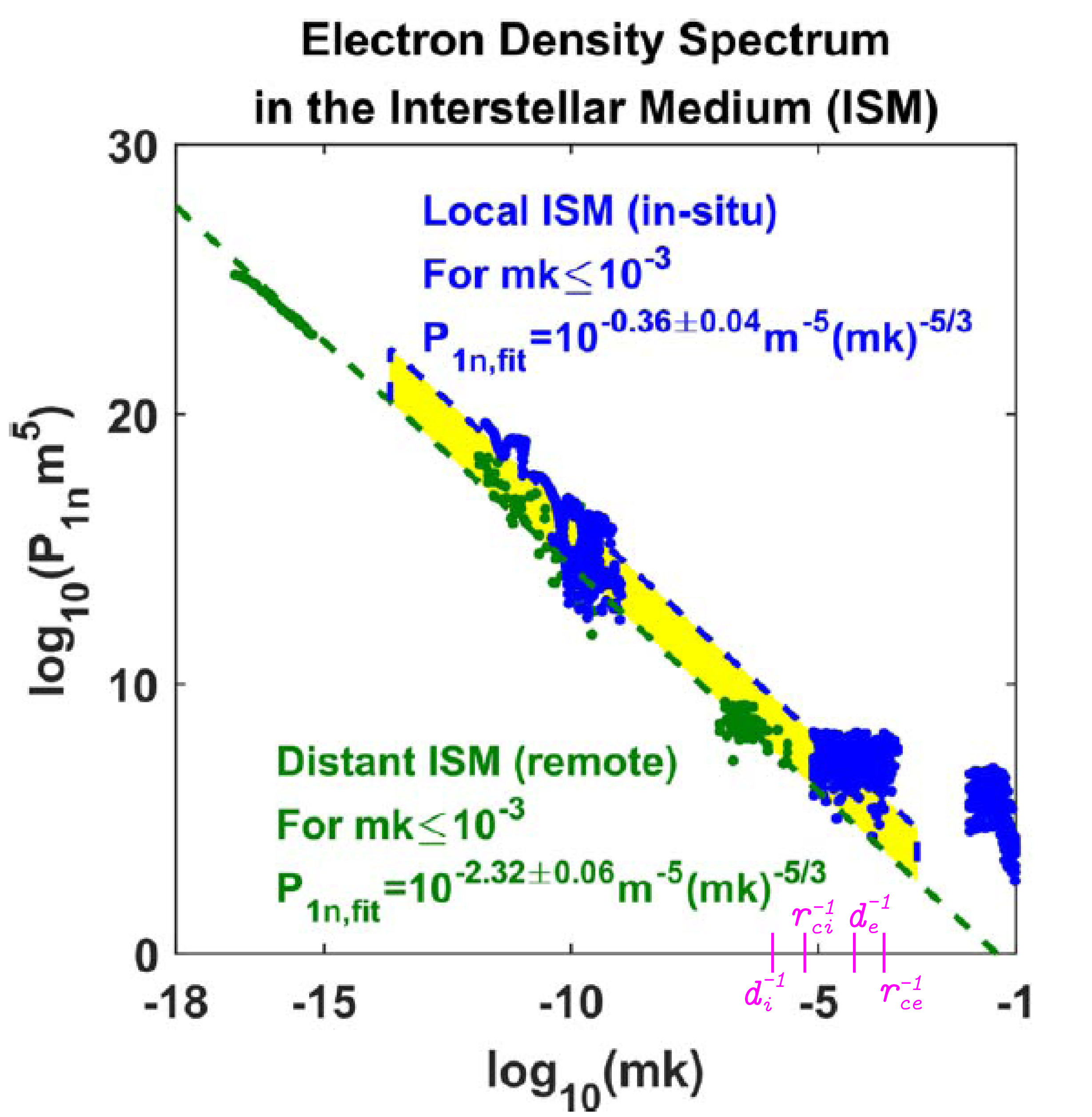
6.2 In situ observations of electron density fluctuations in the VLISM
Recently, Lee and Lee (2019), Lee and Lee (2020) and Ocker et al. (2021b) computed spectral density functions (SDFs) of electron density fluctuations using V1 PWS data, and compared them with the far ISM spectrum. Both enhanced plasma wave events and the recently discovered continuous emission line (Ocker et al., 2021a) have been used for the analysis. To date, these are the only available observations in the kinetic regime, at scales as small as m. The physical mechanisms responsible for the persistent plasma waves is not entirely clear, but Gurnett et al. (2021) suggested that the emission is driven by suprathermal electrons that excite Langmuir waves, with minimum wavelength –2300 m and phase speed km s-1. These oscillations are comparable to the quasi-thermal noise (QTN) but, according to Gurnett et al. (2021), QTN from a Maxwellian electron velocity distribution (with either K or 30,000 K) cannot be detected by the effective 7.1 m dipole antenna of Voyager, since the Debye length is estimated to be 35 m. Figure 29(top) from their study shows that a core-Maxwellian and kappa distribution may explain V1 PWS observations (bottom panel). In this case, suprathermal electrons may contribute significantly to the pressure in the VLISM. Meyer-Vernet et al. (2022) instead predict that a minute concentration of suprathermal electrons, may be sufficient to explain the observed V1 emission line. What is the origin of the suprathermal tail? Is the narrowband emission caused by Brownian-motion-like fluctuations in the phase-space density of the high-energy tail, or it is due to fluctuations caused by the a turbulent cascade? These questions are subject to current scientific debate.
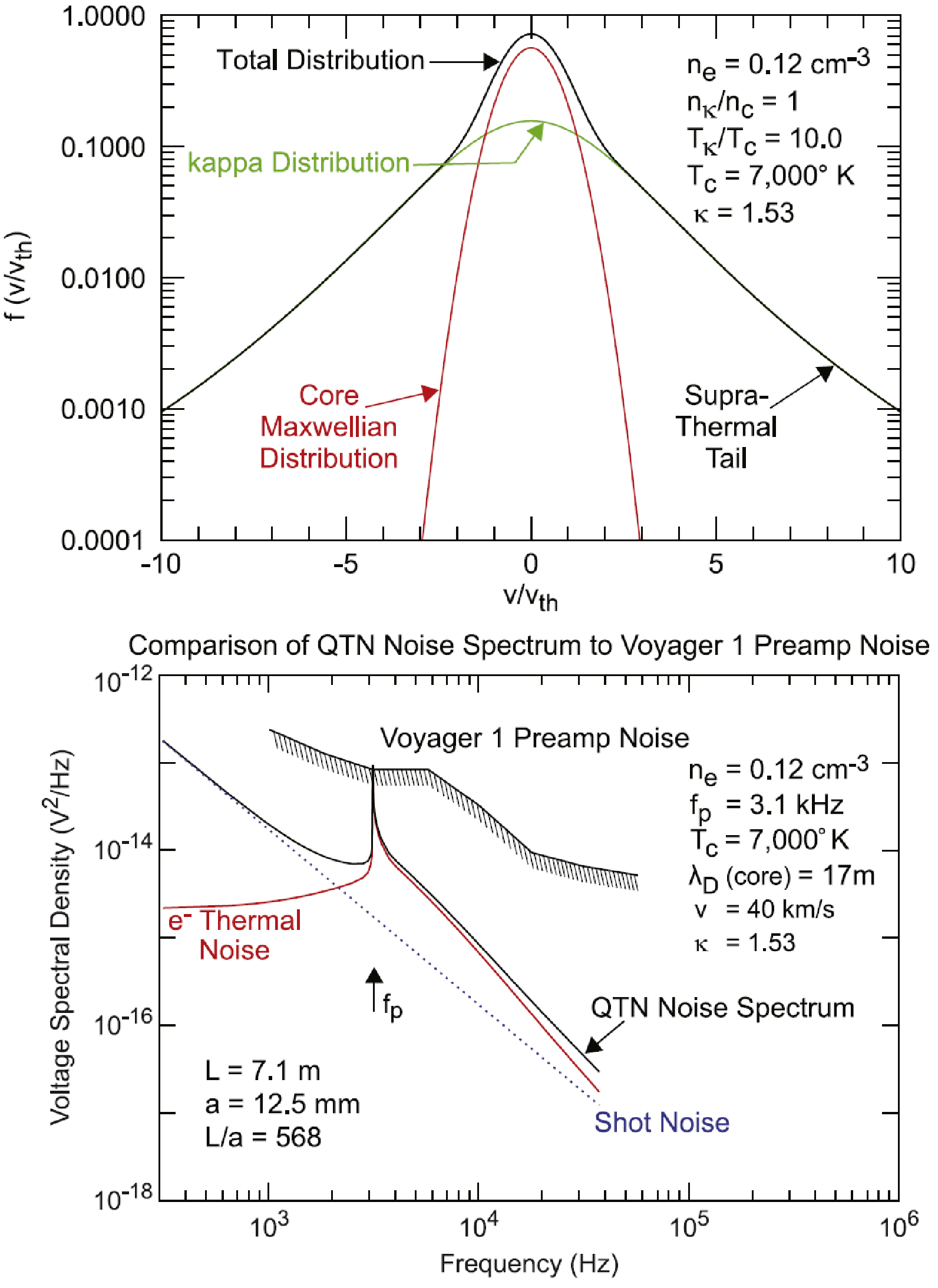
The SDF obtained by Lee and Lee (2020) is shown in Fig. 28. At kinetic scales, a bulge of enhanced power is observed at m-1 (), which can indicate the presence of high frequency wave activity that may include Langmuir waves, ion and electron cyclotron waves, mirror waves, or compressive kinetic Alfvén waves. The shallower spectral slope at such scales was also found by Ocker et al. (2021b), who also warn about the possibility that quantization of the PWS data in this regime might bias the density fluctuations. At MHD scales ( m-1), the in situ spectrum obtained in the VLISM by Lee and Lee (2020) follows a Kolmogorov-like power law (), and its intensity is higher than the remote spectrum of Armstrong et al. (1995) by a factor of (). The power excess of in situ data was later confirmed by Ocker et al. (2021b) and is consistent with the presence of compression waves. Ocker et al. (2021b) have also investigated the electron density turbulence near the Guitar Nebula and other stellar bow shocks, providing evidence that density fluctuations near such bow shocks may be significantly amplified with respect to the diffuse, warm ionized medium.
6.3 Microinstability of PUI distributions and the IBEX ribbon
A kinetic process expected to take place in the VLISM is the instability of the ring-beam distributions of PUIs born in the VLISM by charge exchange between SW neutrals and VLISM ions. The issue of PUI isotropization in the VLISM is still highly debated. Models predict that the ring-beam distribution is subject to a number of instabilities such as beam-driven Alfvén ion cyclotron (AIC), mirror and ion Bernstein (IB), magnetosonic, ion-ion beam-core modes, reviewed by Gary (1991, 1993); Gary et al. (1984). Hybrid simulations and instability analysis have been presented, e.g., by Florinski et al. (2010); Summerlin et al. (2014); Florinski et al. (2016); Min and Liu (2018); Roytershteyn et al. (2019); Mousavi et al. (2020). Florinski et al. (2016) discovered a stability gap for the AIC instability. However, here mirror and IB modes may be unstable, as shown by Min and Liu (2018). Roytershteyn et al. (2019) simulated realistic pickup ion distributions inferred from the MS-FLUKSS global model. They found that the instability reaches the saturation condition on short time scales of hours or days, with low magnetic fluctuation amplitudes, but no isotropization was achieved on the time scales accessible to the simulations. Recently, Mousavi et al. (2020) explored the excitation of possible oblique instabilities using the same distributions of Roytershteyn et al. (2019) and a larger 2D simulation domain. They have shown that mirror mode waves are also unstable, initially with a larger growth rate than AIC waves. The mirror modes were reported to produce additional scattering of PUIs and to eventually result in additional growth of AIC waves that dominate late in the simulations. It is important to emphasize that majority of existing simulations report behavior on relatively short time scales (compared to the charge exchange time in the VLISM, see below). A longer time-evolution is likely accessible only to quasi-linear analysis of the type undertaken by Min and Liu (2018), rather than to direct kinetic simulations.
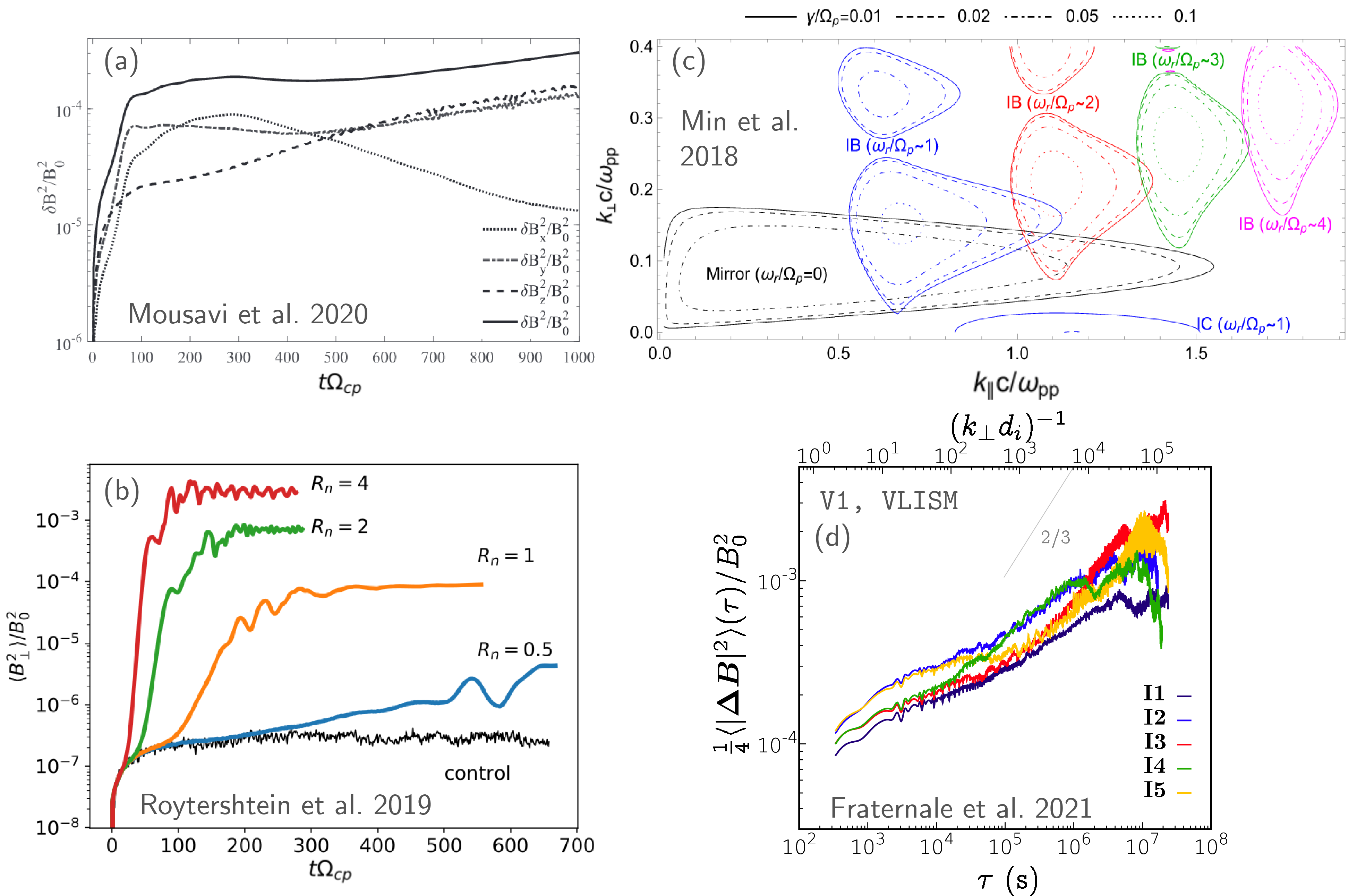
Can Voyager observe signatures of PUI self-generated turbulence? The above studies agree in that the range of parallel wavenumbers of interest for the instability is .
As shown in Fig. 27(a) and Fig. 30(d), such a wavenumber range may have been partially observed by V1. The above studies agree that the instability amplitudes at saturation conditions are in the range of , for realistic PUI densities. Burlaga and Ness (2014b) and Florinski et al. (2016) compared the instability amplitudes with V1 observations and estimated that the instability amplitude should be much larger than the level of turbulence observed by Voyager. However, this conclusion had to be revised because of a normalization error in the PSDs of Burlaga et al. (2015). A new comparison has been made recently by Fraternale and Pogorelov (2021). Interestingly, the normalized intensity of magnetic field fluctuations at V1 in the VLISM seems to be compatible with the expected amplitudes of PUI waves. Panels (a) and (b) of Fig. 30 report the normalized amplitude of self-generated turbulence in the hybrid simulations of Roytershteyn et al. (2019) and Mousavi et al. (2020). Panel (d) shows the normalized 2nd–order structure functions of magnetic field fluctuations in different intervals at V1 from 288 s averaged data. Since Voyager MAG measurements in the microscale regime lie in the noisy band and are very close to the sensitivity of the magnetometers, further investigations are needed to draw conclusions on this topic.
The VLISM turbulence and the instability process of PUI distributions are both key ingredients of the existing theories for the formation of the IBEX “ribbon” of enhanced ENAs, as discussed in Sec. 3.2.3 of Galli et al. (2022) in this volume.
Essentially, the fundamental and still open question is whether a quasi-anisotropic PUI pitch angle distribution in space can be reached in the VLISM, what is the role of preexisting turbulence and kinetic instabilities in the isotropization of the PUI distribution, and what is the typical time scale of the isotropization, as compared to the charge exchange collision rate.
Both the weak scattering (e.g., Zirnstein et al., 2018, and references therein) and the strong scattering limits have been considered. In the latter case, one theory predicts that the ribbon is formed within a “retention region”, in directions perpendicular to the ISMF, where newly ionized atoms are temporarily contained due to the enhanced scattering by the local turbulence (Schwadron and McComas, 2013; Isenberg, 2014; Schwadron et al., 2018). Giacalone and Jokipii (2015) suggested that magnetic mirroring may play an important role in trapping particles in pre-existing, small-amplitude compressible turbulence. Zirnstein et al. (2020) extended the work of Giacalone and Jokipii (2015) by simulating the 3D transport of PUI in the VLISM in the presence of Kolmogorov-like, homogeneous, and isotropic turbulence with a power spectrum that fits V1 observations by Burlaga et al. (2018). Interestingly, it was found that the structure of the ribbon can be well reproduced only if the magnetic turbulence correlation scale is smaller than 50 AU. This result is consistent with the idea that the ribbon source lies within a few tens of AU from the HP (Swaczyna et al., 2016), and fits well the turbulence scenario the that is emerging from the recent studies.
7 Magnetic reconnection
It has long been suggested that magnetic reconnection at the heliopause may play a significant role in determining the overall morphology of the magnetic field, as well as the plasma transport across the heliopause (e.g. Fahr et al., 1986). Indeed, simulations of Pogorelov et al. (2017b) confirmed that the HP is subject to MHD instabilities and magnetic reconnection (see Fig. 31, left panel). Further, the sector structure of the HMF in the IHS is inherently favorable to magnetic reconnection due to both the compression of sectors and the increase of with distance (right panel in Fig. 31), which may play a role in accelerating ACRs (e.g. Lazarian and Opher, 2009; Drake et al., 2010; Opher et al., 2011).
As discussed by Burlaga et al. (2020a), there is no compelling direct evidence in Voyager data for magnetic reconnection, even in the distant IHS. On the other hand, observations alone are not sufficient to conclude that magnetic reconnection does not occur and, arguably, reconnection cannot really be separated from turbulence (Lazarian and Vishniac, 1999; Eyink et al., 2011; Eyink, 2015). Some of the principal points of discussion in the literature on magnetic reconnection in the IHS include:
-
1.
The magnetic flux apparent decrease at V1, not observed at V2 (Burlaga et al., 2019b). We emphasize that this flux should be conserved only for a radial, steady flow, and azimuthal magnetic field, in absence of dissipative processes. None of these conditions are actually satisfied in the IHS. On the other hand, Drake et al. (2017) have shown that the magnetic flux is not necessarily reduced in a reconnecting current layer.
-
2.
A few “D-sheets”, supposed to be a manifestation of reconnection in the supersonic SW, have been observed in the IHS (Burlaga et al., 2006a; Burlaga and Ness, 2009; Burlaga et al., 2017). Such events are rare in the data, but it may not be surprising because the spacecraft sample a tiny portion of space and time.
-
3.
Less HCS crossings than expected have been detected at V1 (Richardson et al., 2016)
- 4.
-
5.
The HMF magnitude near the HP obtained from global simulations is in agreement with observations only in time dependent simulations where the HCS is allowed to dissipate (by numerical viscosity). In the assumption of unipolar HMF, its strength in the IHS is 5-7 times stronger than observed (see Pogorelov et al., 2021; Kleimann et al., 2022). This suggests that HMF dissipation occurs in the real system but quantifying the dissipation rate and pathways remains a challenge.
Description of magnetic reconnection in the IHS and at the HP is an extremely difficult problem in both global and kinetic models. Indeed, significant progress has been achieved in recent decades in understanding of magnetic reconnection in weakly collisional plasma, such as the solar wind (e.g. Yamada et al., 2010; Ji and Daughton, 2011; Burch et al., 2016). At the most fundamental level, the reconnection in such regimes proceeds by compressing current sheets—the regions of very large magnetic shear—all the way down to electron scales. However, in high Reynolds number systems turbulence, either self-generated or pre-existing, plays an essential role (e.g. Lazarian and Vishniac, 1999; Eyink et al., 2011; Eyink, 2015; Daughton and Roytershteyn, 2012; Lazarian et al., 2020, and references therein) to enable magnetic reconnection on global scales. Such a coupling between microscopic and macroscopic dynamics is impossible to describe in global models.
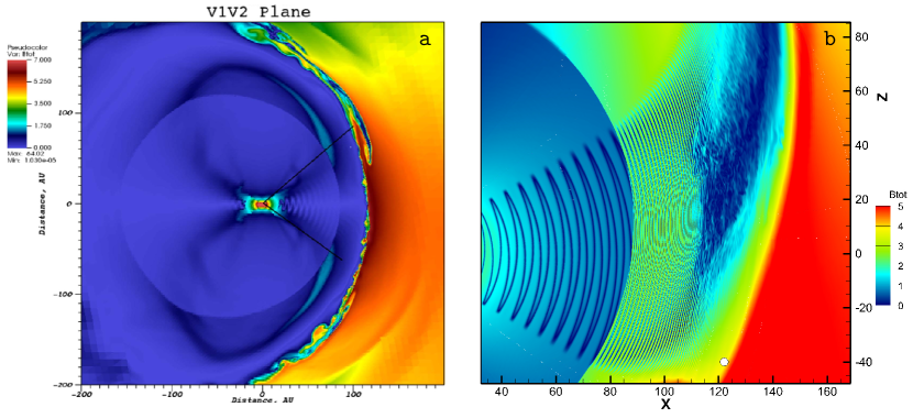
Even the influence of turbulence may be difficult to capture properly due to the limited resolution of such models. The only feasible approach consists of identifying potential reconnection sites in global models based on simple analytical criteria (such as large shear of magnetic field) and then studying these regions using local models with boundary and driving conditions corresponding to the regions of interest. It is beneficial to employ kinetic formalism in the local simulations and utilize fully kinetic and hybrid kinetic (kinetic ions + fluid electrons) particle-in-cell codes to study magnetic reconnection on microscopic (below 100 ) and mesoscopic scales (up to ).
Even though the PUIs have relatively low density in the regions of interest, they are energetically dominant beyond the HTS. Meanwhile, previous investigations of magnetic reconnection in the IHS and at the HP either ignored the presence of PUIs, or modeled them in highly simplified manner (e.g. as an isotropic Maxwellian population with higher temperature than the background (e.g. as an isotropic Maxwellian population with higher temperature than the background, Drake et al., 2010). Some relevant clues to the possible influence of PUIs are offered by the previous investigations of the role played by heavy ions, in particular O+, in the reconnection process in the Earth’s magnetosphere. Such investigations revealed existence of a separate, larger, O+ diffusion region in addition to proton and electron diffusion regions, as well as offered evidence that the presence of O+ may significantly affect reconnection dynamics (Liu et al., 2015). As such, one might expect that PUIs also have a substantial effect on the structure of reconnection regions, onset of reconnection, and other important properties of the reconnection regions.
8 Concluding Remarks
Turbulence is critical to various heliospheric processes accompanying the SW–LISM interaction on scales ranging from AU to the electron kinetic scales.
In this paper, we attempted to give an overview of the evidence of turbulence in the distant, supersonic SW, heliosheath, and VLISM regions. A long-standing problem of identifying the channels of energy transfer and turbulent heating rates of ions and electrons is perhaps the most fundamental open challenge in all regions. Understanding the energy reservoirs in the outer heliosphere is also critical. Energetically dominant PUIs inject turbulent energy at small scales through several instability processes, but large-scale structures, instabilities, and shock waves are also present. At inertial range scales, the study of variance anisotropy measurements at large heliocentric distances have not provided sufficient insight into the geometry of turbulence, which raises a question about the applicability of the “standard” paradigms based on near-Earth observations.
In the IHS and VLISM, the best evidence of turbulence so far has been the observation of intermittency of magnetic field fluctuations, power-law regimes for spectra and higher order structure functions, and multifractal statistics. The prominent feature of turbulence in these regions is its compressible nature. This also constitutes the major challenge from the modeling perspective. Recent theoretical and numerical investigations have provided us with convincing explanations on how the termination shock and the heliopause can generate compressible turbulence in the IHS and VLISM.
However, the mechanisms responsible for the in situ origin of microscale compressible fluctuations are less clear. In the IHS, they have been associated with local temperature-anisotropy-driven instabilities. What is the contribution of these structures to the overall cascade rate? How are large-scale traveling wave modes coupled to turbulence? How do turbulence and reconnection operate to dissipate the HCS, especially near the HP? To date, these questions remain largely unsolved.
Recent studies suggest that the turbulence observed in the VLISM is a superposition of the fluctuations emanated by the HP and the background LISM turbulence. However, discriminating between these two components has not been possible so far, which leaves the question about the properties of the unperturbed LISM turbulence open. Some features of the VLISM turbulence remain obscure. For instance, what is the dissipation rate of compressible turbulence? What is the origin of quasiperiodic oscillations and N-wave profiles observed at MHD scales? What is the role of turbulence in the VLISM shock formation, structure and propagation? What processes are dominant at ion scales and what are the isotropization time scales of suprathermal particle distributions? What is the origin of suprathermal electrons and Langmuir waves? What specific turbulence cascade phenomenology can describe the VLISM turbulence?
We only have partial answers to these questions. Pursuing the investigation of turbulence in the outer heliosphere will allow the space physics community to make a step forward in the understanding of turbulence as a basic physical process. Such progress should shed light on the mechanisms of magnetic field dissipation in the IHS and on the dynamical effects of turbulence on the SW flow.
Acknowledgements.
This work was made possible by the International Space Science Institute and its interdisciplinary workshop “The Heliosphere in the Local Interstellar Medium”222www.issibern.ch/workshops/heliosphere. FF was supported by NASA grants 80NSSC19K0260, 80NSSC18K1649, 80NSSC18K1212. C.W.S. is supported by Advanced Composition Explorer Mission as well as NASA grants NNX17AB86G, 80NSSC17K0009, and 80NSSC18K1215. H.F., J.K., and S.O. acknowledge support for their work within the framework of the DFG (Deutsche Forschungsgemeinschaft) grant FI 706/23-1. NP was supported, in part, by NASA grants 80NSSC19K0260, 80NSSC18K1649, 80NSSC18K1212, NSF-BSF grant PHY-2010450, and by the IBEX mission as a part of NASA’s Explorer program. GPZ, LA, and LZ acknowledge the partial support of the NSF EPSCoR RII-Track-1 Cooperative Agreement OIA-1655280.References
- Adhikari et al. (2014) Adhikari L, Zank GP, Hu Q, Dosch A (2014) Turbulence transport modeling of the temporal outer heliosphere. Astrophys. J.793:52, DOI 10.1088/0004-637X/793/1/52
- Adhikari et al. (2015) Adhikari L, Zank GP, Bruno R, Telloni D, Hunana P, Dosch A, Marino R, Hu Q (2015) The transport of low-frequency turbulence in astrophysical flows. II. Solutions for the super-Alfvénic solar wind. Astrophys J 805(1):63, DOI 10.1088/0004-637x/805/1/63
- Adhikari et al. (2017) Adhikari L, Zank GP, Hunana P, Shiota D, Bruno R, Hu Q, Telloni D (2017) II. Transport of nearly incompressible magnetohydrodynamic turbulence from 1 to 75 au. Astrophys J 841(2):85, DOI 10.3847/1538-4357/aa6f5d
- Adhikari et al. (2017) Adhikari L, Zank GP, Telloni D, Hunana P, Bruno R, Shiota D (2017) Theory and transport of nearly incompressible magnetohydrodynamics turbulence. III. Evolution of power anistropy in magnetic field fluctuations throughout the heliosphere. Astrophys. J.851:117, DOI 10.3847/1538-4357/aa9ce4
- Adhikari et al. (2019) Adhikari L, Zank GP, Zhao LL (2019) Does turbulence turn off at the Alfvén critical surface? Astrophys. J.876(1):26, DOI 10.3847/1538-4357/ab141c
- Adhikari et al. (2021) Adhikari L, Zank GP, Zhao LL (2021) The transport and evolution of MHD turbulence throughout the heliosphere: Models and observations. Fluids 6, DOI 10.3390/fluids6100368
- Alexandrova et al. (2008) Alexandrova O, Carbone V, Veltri P, Sorriso-Valvo L (2008) Small-scale energy cascade of the solar wind turbulence. Astrophys J 674(2):1153–1157, DOI 10.1086/524056
- Alexandrova et al. (2009) Alexandrova O, Saur J, Lacombe C, Mangeney A, Mitchell J, Schwartz SJ, Robert P (2009) Universality of solar-wind turbulent spectrum from MHD to electron scales. Phys Rev Lett 103:165003, DOI 10.1103/PhysRevLett.103.165003
- Alexandrova et al. (2012) Alexandrova O, Lacombe C, Mangeney A, Grappin R, Maksimovic M (2012) Solar wind turbulent spectrum at plasma kinetic scales. Astroph J 760(2), DOI 10.1088/0004-637X/760/2/121
- Alexandrova et al. (2013) Alexandrova O, Chen CHK, Sorriso-Valvo L, Horbury TS, Bale SD (2013) Solar wind turbulence and the role of ion instabilities. Space Science Reviews 178(2-4):101–139, DOI 10.1007/s11214-013-0004-8
- Armstrong et al. (1981) Armstrong JW, Cordes J, Rickett B (1981) Density power spectrum in the local interstellar medium. Nature 291:561–564, DOI 10.1038/291561a0
- Armstrong et al. (1995) Armstrong JW, Rickett BJ, Spangler SR (1995) Electron density power spectrum in the local interstellar medium. Astrophys J 443(1):209–221, DOI 10.1086/175515
- Avinash and Zank (2007) Avinash K, Zank GP (2007) Magnetic structures in the heliosheath. Geophys Res Lett 34(5):L05106, DOI 10.1029/2006GL028582
- Avinash et al. (2014) Avinash K, Zank GP, Dasgupta B, Bhadoria S (2014) Instability of the heliopause driven by charge exchange interactions. Astrophys J 791(2):102, DOI 10.1088/0004-637x/791/2/102
- Bale et al. (2019) Bale S, Badman S, Bonnell Jea (2019) Highly structured slow solar wind emerging from an equatorial coronal hole. Nature 576:237–242, DOI 10.1038/s41586-019-1818-7
- Bale et al. (2005) Bale SD, Kellogg PJ, Mozer FS, Horbury TS, Reme H (2005) Measurement of the electric fluctuation spectrum of magnetohydrodynamic turbulence. Phys Rev Lett 94:215002, DOI 10.1103/PhysRevLett.94.215002
- Banerjee and Galtier (2013) Banerjee S, Galtier S (2013) Exact relation with two-point correlation functions and phenomenological approach for compressible magnetohydrodynamic turbulence. Phys Rev E 87:013019, DOI 10.1103/PhysRevE.87.013019
- Baranov and Ruderman (2013) Baranov VB, Ruderman MS (2013) On the effect of transport coefficient anisotropy on the plasma flow in heliospheric interface. M Not R Astron Soc 434(4):3202–3207, DOI 10.1093/mnras/stt1267
- Baranov et al. (1979) Baranov VB, Lebedev MG, Ruderman MS (1979) Structure of the region of solar wind—interstellar medium interaction and its influence on H atoms penetrating the solar wind. Astrophys Space Sci 66(2):441–451
- Baranov et al. (1992) Baranov VB, Fahr HJ, Ruderman MS (1992) Investigation of macroscopic instabilities at the heliopause boundary surface. Astron Astrophys 261(1):341–347
- Batchelor (1959) Batchelor GK (1959) Small-scale variation of convected quantities like temperature in turbulent fluid part 1. General discussion and the case of small conductivity. J Fluid Mech 5(1):113–133, DOI 10.1017/S002211205900009X
- Bavassano and Bruno (1991) Bavassano B, Bruno R (1991) Solar wind fluctuations at large scale: A comparison between low and high solar activity conditions. J. Geophys. Res.96(A2):1737–1744, DOI 10.1029/90JA01959
- Behannon et al. (1977) Behannon KW, Acuna MH, Burlaga LF, Lepping RP, Ness NF, Neubauer FM (1977) Magnetic field experiment for Voyagers 1 and 2. Space Sci Rev 21(3):235–257
- Belcher and Davis (1971) Belcher JW, Davis L (1971) Large-amplitude Alfvén waves in the interplanetary medium, 2. J Geophys Res 76(16):3534–3563, DOI 10.1029/JA076i016p03534
- Belov and Myasnikov (1999) Belov NA, Myasnikov AV (1999) Instability of a contact surface separating two hypersonic source flows. Fluid Dynamics 34:379–387, DOI 10.1103/PhysRevE.48.R29
- Benzi et al. (1993) Benzi R, Ciliberto S, Tripiccione R, Baudet C, Massaioli F, Succi S (1993) Extended self-similarity in turbulent flows. Phys Rev E 48(1):R29–R32, DOI 10.1103/PhysRevE.48.R29
- Berdichevsky (2009) Berdichevsky DB (2009) Voyager mission, detailed processing of weak magnetic fields; i constraints to the uncertainties of the calibrated magnetic field signal in the Voyager missions. white paper URL https://vgrmag.gsfc.nasa.gov/20151017BzPLestimates\_wMAGCAL.pdf
- Beresnyak (2012) Beresnyak A (2012) Basic properties of magnetohydrodynamic turbulence in the inertial range. M Not R Astron Soc 422(4):3495–3502, DOI 10.1111/j.1365-2966.2012.20859.x
- Beresnyak and Lazarian (2015) Beresnyak A, Lazarian A (2015) MHD Turbulence, turbulent dynamo and applications, Springer, Chap 8
- Beresnyak and Lazarian (2019) Beresnyak A, Lazarian A (2019) Turbulence in Magnetohydrodynamics. De Gruyter, DOI doi:10.1515/9783110263282
- Bieber et al. (1996) Bieber JW, Wanner W, Matthaeus WH (1996) Dominant two-dimensional solar wind turbulence with implications for cosmic ray transport. J Geophys Res 101(A2):2511–2522, DOI 10.1029/95JA02588
- Biskamp (2003) Biskamp D (2003) Magnetohydrodynamic turbulence. Cambridge University Press
- Bochsler et al. (2013) Bochsler P, Kucharek H, Möbius E, Bzowski M, Sokół JM, Didkovsky L, Wieman S (2013) Solar photoionization rates for interstellar neutrals in the inner heliosphere: H, He, O, and Ne. Astrophysical J Supp Ser 210(1):12, DOI 10.1088/0067-0049/210/1/12
- Boldyrev (2005) Boldyrev S (2005) On the spectrum of magnetohydrodynamic turbulence. Astrophys J 626(1,2):L37–L40
- Boldyrev (2006) Boldyrev S (2006) Spectrum of magnetohydrodynamic turbulence. Phys Rev Lett 96:115002, DOI 10.1103/PhysRevLett.96.115002
- Borovikov and Pogorelov (2014) Borovikov SN, Pogorelov NV (2014) Voyager 1 near the heliopause. Astrophys J Lett 783(1), DOI 10.1088/2041-8205/783/1/L16
- Borovikov et al. (2008) Borovikov SN, Pogorelov NV, Zank GP, Kryukov IA (2008) Consequences of the heliopause instability caused by charge exchange. Astrophys J 682(2):1404–1415, DOI 10.1086/589634
- Borovikov et al. (2011) Borovikov SN, Pogorelov NV, Burlaga LF, Richardson JD (2011) Plasma near the heliosheath: observations and modeling. Astrophys J Lett 728(1), DOI 10.1088/2041-8205/728/1/L21
- Borovikov et al. (2012) Borovikov SN, Pogorelov NV, Ebert RW (2012) Solar rotation effects on the heliosheath flow near solar minima. Astrophys J 750(1), DOI 10.1088/0004-637X/750/1/42
- Borovsky (2008) Borovsky JE (2008) Flux tube texture of the solar wind: Strands of the magnetic carpet at 1 au? J Geophys Res 113(A8):A08110, DOI 10.1029/2007JA012684
- Borrmann and Fichtner (2005) Borrmann T, Fichtner H (2005) On the dynamics of the heliosphere on intermediate and long time-scales. Adv Space Res 35(12):2091–2101, DOI 10.1016/j.asr.2005.08.039
- Bowen et al. (2020a) Bowen TA, Mallet A, Bale SD, Bonnell JW, Case AW, Chandran BDG, Chasapis A, Chen CHK, Duan D, Dudok de Wit T, Goetz K, Halekas JS, Harvey PR, Kasper JC, Korreck KE, Larson D, Livi R, MacDowall RJ, Malaspina DM, McManus MD, Pulupa M, Stevens M, Whittlesey P (2020a) Constraining ion-scale heating and spectral energy transfer in observations of plasma turbulence. Phys Rev Lett 125:025102, DOI 10.1103/PhysRevLett.125.025102, URL https://link.aps.org/doi/10.1103/PhysRevLett.125.025102
- Bowen et al. (2020b) Bowen TA, Mallet A, Huang J, Klein KG, Malaspina DM, Stevens M, Bale SD, Bonnell JW, Case AW, Chandran BDG, Chaston CC, Chen CHK, de Wit TD, Goetz K, Harvey PR, Howes GG, Kasper JC, Korreck KE, Larson D, Livi R, MacDowall RJ, McManus MD, Pulupa M, Verniero JL, Whittlesey P, the PSP teams (2020b) Ion-scale electromagnetic waves in the inner heliosphere. Astrophys J Suppl Ser 246(2):66, DOI 10.3847/1538-4365/ab6c65
- Breech et al. (2005) Breech B, Matthaeus WH, Minnie J, Oughton S, Parhi S, Bieber JW, Bavassano B (2005) Radial evolution of cross helicity in high-latitude solar wind. Geophys Res Lett 32(6), DOI 10.1029/2004GL022321
- Breech et al. (2008) Breech B, Matthaeus WH, Minnie J, Bieber JW, Oughton S, Smith CW, Isenberg PA (2008) Turbulence transport throughout the heliosphere. J Geophys Res: Space Physics 113(A8), DOI 10.1029/2007JA012711
- Breech et al. (2009) Breech B, Matthaeus WH, Cranmer SR, Kasper JC, Oughton S (2009) Electron and proton heating by solar wind turbulence. J Geophys Res: Space Physics 114(A9), DOI 10.1029/2009JA014354
- Bruno and Carbone (2013) Bruno R, Carbone V (2013) The solar wind as a turbulence laboratory. Living Rev Solar Phys 10(2), DOI 10.12942/lrsp-2013-2
- Burch et al. (2016) Burch JL, Torbert RB, Phan TD, Chen LJ, Moore TE, Ergun RE, Eastwood JP, Gershman DJ, Cassak PA, Argall MR, Wang S, Hesse M, Pollock CJ, Giles BL, Nakamura R, Mauk BH, Fuselier SA, Russell CT, Strangeway RJ, Drake JF, Shay MA, Khotyaintsev YV, Lindqvist PA, Marklund G, Wilder FD, Young DT, Torkar K, Goldstein J, Dorelli JC, Avanov LA, Oka M, Baker DN, Jaynes AN, Goodrich KA, Cohen IJ, Turner DL, Fennell JF, Blake JB, Clemmons J, Goldman M, Newman D, Petrinec SM, Trattner KJ, Lavraud B, Reiff PH, Baumjohann W, Magnes W, Steller M, Lewis W, Saito Y, Coffey V, Chandler M (2016) Electron-scale measurements of magnetic reconnection in space. Science 352(6290):aaf2939, DOI 10.1126/science.aaf2939
- Burgess et al. (2016) Burgess D, Hellinger P, Gingell I, Trávníček PM (2016) Microstructure in two- and three-dimensional hybrid simulations of perpendicular collisionless shocks. Journal of Plasma Physics 82(04):905820401, DOI 10.1017/S0022377816000660
- Burlaga and Ness (2011) Burlaga L, Ness N (2011) Current sheets in the heliosheath: Voyager 1, 2009. J Geophys Res: Space Physics 116(A5), DOI 10.1029/2010JA016309
- Burlaga et al. (2019a) Burlaga L, Ness NF, Berdichevsky D, Park J, Jian L, Szabo A, Stone E, Richardson J (2019a) Magnetic field and particle measurements made by Voyager 2 at and near the heliopause. Nature Astronomy 3(11):1007–1012, DOI 10.1038/s41550-019-0920-y
- Burlaga (1968) Burlaga LF (1968) Micro-scale structures in the interplanetary medium. Solar Phys 4(1):67–92, DOI 10.1007/BF00146999
- Burlaga (1991) Burlaga LF (1991) Multifractal structure of the interplanetary magnetic field: Voyager 2 observations near 25 au, 1987-1988. Geophys Res Lett 18(1):69–72, DOI 10.1029/90GL02596
- Burlaga (1994) Burlaga LF (1994) Merged interaction regions and large-scale magnetic field fluctuations during 1991 - Voyager-2 observations. J Geophys Res 99:19341–19350, DOI 10.1029/94JA01513
- Burlaga (1995) Burlaga LF (1995) Interplanetary magnetohydrodynamics. Oxford University Press
- Burlaga (2001) Burlaga LF (2001) Lognormal and multifractal distributions of the heliospheric magnetic field. J Geophys Res 106(A8):15917–15927, DOI 10.1029/2000JA000107
- Burlaga (2004) Burlaga LF (2004) Multifractal structure of the large-scale heliospheric magnetic field strength fluctuations near 85au. Nonl Proc Geophys 11(4):441–445, DOI 10.5194/npg-11-441-2004
- Burlaga and Ness (2009) Burlaga LF, Ness NF (2009) Compressible “turbulence” observed in the heliosheath by Voyager 2. Astrophys J 703(1):311, DOI 10.1088/0004-637X/703/1/311
- Burlaga and Ness (2010) Burlaga LF, Ness NF (2010) Sectors and large-scale magnetic field strength fluctuations in the heliosheath near 110 au: Voyager 1, 2009. Astrophys J 725(1):1306, DOI 10.1088/0004-637X/725/1/1306
- Burlaga and Ness (2012) Burlaga LF, Ness NF (2012) Magnetic field fluctuations observed in the heliosheath by Voyager 1 at 114 2 au during 2010. J Geophys Res 117:A10107, DOI 10.1029/2012JA017894
- Burlaga and Ness (2012) Burlaga LF, Ness NF (2012) Magnetic field strength fluctuations in the heliosheath: Voyager 1 observations during 2009. Astrophys J 744(1):51, DOI 10.1088/0004-637X/744/1/51
- Burlaga and Ness (2013) Burlaga LF, Ness NF (2013) Magnetic field strength fluctuations and the q-triplet in the heliosheath: Voyager 2 observations from 91.0 to 94.2 au at latitude 30?? s. Astrophys J 765(1):35, DOI 10.1088/0004-637X/765/1/35
- Burlaga and Ness (2014a) Burlaga LF, Ness NF (2014a) Interstellar magnetic fields observed by Voyager 1 beyond the heliopause. Astrophys J Lett 795(1), DOI 10.1088/2041-8205/795/1/L19
- Burlaga and Ness (2014b) Burlaga LF, Ness NF (2014b) Voyager 1 observations of the interstellar magnetic field and the transition from the heliosheath. Astrophys J 784:146, DOI 10.1088/0004-637X/784/2/146
- Burlaga and Ness (2016) Burlaga LF, Ness NF (2016) Observations of the interstellar magnetic field in the outer heliosheath: Voyager 1. Astrophys J 829(2):134, DOI 10.3847/0004-637X/829/2/134
- Burlaga et al. (1996) Burlaga LF, Ness NF, Belcher JW, Whang YC (1996) Pickup protons and pressure-balanced structures from 39 to 43 au: Voyager 2 observations during 1993 and 1994. J Geophys Res 101(A7):15523–15532, DOI 10.1029/96JA01076
- Burlaga et al. (2002) Burlaga LF, Ness NF, Wang YM, Sheeley NR (2002) Heliospheric magnetic field strength and polarity from 1 to 81 au during the ascending phase of solar cycle 23. J Geophys Res 107:1410–19350, DOI 10.1029/2001JA009217
- Burlaga et al. (2003a) Burlaga LF, Wang C, Ness NF (2003a) A model and observations of the multifractal spectrum of the heliospheric magnetic field strength fluctuations near 40 au. Geophys Res Lett 30(10), DOI 10.1029/2003GL016903
- Burlaga et al. (2003b) Burlaga LF, Wang C, Richardson JD, Ness NF (2003b) Evolution of magnetic fields in corotating interaction regions from 1 to 95 au: Order to chaos. Astrophys J 590(1, 1):554–566, DOI 10.1086/374926
- Burlaga et al. (2003c) Burlaga LF, Wang C, Richardson JD, Ness NF (2003c) Evolution of the multiscale statistical properties of corotating streams from 1 to 95 au. J Geophys Res 108(A7), DOI 10.1029/2003JA009841
- Burlaga et al. (2006a) Burlaga LF, Ness NF, Acuna MH (2006a) Magnetic fields in the heliosheath: Voyager 1 observations. Astrophys J 642(1):584, DOI 10.1086/500826
- Burlaga et al. (2006b) Burlaga LF, Ness NF, Acuna MH (2006b) Multiscale structure of magnetic fields in the heliosheath. J Geophys Res-Space Physics 111(A9), DOI 10.1029/2006JA011850
- Burlaga et al. (2007) Burlaga LF, F-Viñas A, Wang C (2007) Tsallis distributions of magnetic field strength variations in the heliosphere: 5 to 90 au. J Geophys Res 112(A7), DOI 10.1029/2006JA012213
- Burlaga et al. (2008) Burlaga LF, Ness N, Acuña M (2008) Magnetic fields at the solar wind termination shock. Nature 454:75–77, DOI 10.1038/nature07029
- Burlaga et al. (2009) Burlaga LF, Ness NF, Acuna MH, Wang YM, Sheeley NR Jr (2009) Radial and solar cycle variations of the magnetic fields in the heliosheath: Voyager 1 observations from 2005 to 2008. J Geophys Res - Space Phys 114, DOI 10.1029/2009JA014071
- Burlaga et al. (2010) Burlaga LF, Ness NF, Wang YM, Sheeley Jr NR, Richardson JD (2010) Observations of the magnetic field and plasma in the heliosheath by Voyager 2 from 2007.7 to 2009.4. J Geophys Res 115(A8), DOI 10.1029/2009JA015239
- Burlaga et al. (2011) Burlaga LF, Ness NF, Stone E, McDonald FB (2011) Voyager observations of magnetic fields and cosmic rays in the heliosheath. J Geophys Res 116(A12), DOI 10.1029/2011JA016914
- Burlaga et al. (2013a) Burlaga LF, Ness NF, Gurnett DA, Kurth WS (2013a) Evidence for a shock in interstellar plasma: Voyager 1. Astrophys J Lett 778(1), DOI 10.1088/2041-8205/778/1/L3
- Burlaga et al. (2013b) Burlaga LF, Ness NF, Stone EC (2013b) Magnetic field observations as Voyager 1 entered the heliosheath depletion degion. Science 341(6142):147–150, DOI 10.1126/science.1235451
- Burlaga et al. (2014) Burlaga LF, Ness NF, Florinski V, Heerikhuisen J (2014) Magnetic field fluctuations observed in the heliosheath and interstellar magnetic field by Voyager 1 at 115.7-124.9 au during 2011-2013. Astrophys J 792(2):134, DOI 10.1088/0004-637x/792/2/134
- Burlaga et al. (2015) Burlaga LF, Florinski V, Ness NF (2015) In situ observations of magnetic turbulence in the local interstellar medium. Astrophys J Lett 804(2), DOI 10.1088/2041-8205/804/2/L31
- Burlaga et al. (2016) Burlaga LF, Ness NF, Richardson JD, Decker RB, Krimigis SM (2016) Heliosheath magnetic field and plasma observed by Voyager 2 during 2012 in the rising phase of solar cycle 24. Astrophys J 818(2):147, DOI 10.3847/0004-637x/818/2/147
- Burlaga et al. (2017) Burlaga LF, Ness NF, Richardson JD (2017) Transition from the unipolar region to the sector zone: Voyager 2, 2013 and 2014. Asptrophys J 841(1), DOI 10.3847/1538-4357/aa6f5c
- Burlaga et al. (2018) Burlaga LF, Florinski V, Ness NF (2018) Turbulence in the outer heliosheath. Astrophys J 854(1):20, DOI 10.3847/1538-4357/aaa45a
- Burlaga et al. (2019b) Burlaga LF, Ness NF, Berdichevsky DB, Jian LK, Park J, Mostafavi P, Richardson JD (2019b) A magnetic pressure front upstream of the heliopause and the heliosheath magnetic fields and plasma, observed during 2017. Astrophys J 877(1):31, DOI 10.3847/1538-4357/ab16f1
- Burlaga et al. (2020a) Burlaga LF, Ness NF, Berdichevsky DB, Jian LK, Park J, Szabo A (2020a) Intermittency and q-gaussian distributions in the magnetic field of the very local interstellar medium (vlism) observed by Voyager 1 and Voyager 2. Astrophys J Lett 901(1):L2
- Burlaga et al. (2020b) Burlaga LF, Ness NF, Berdichevsky DB, Jian LK, Park J, Szabo A (2020b) Voyager 1 and 2 observations of a change in the nature of magnetic fluctuations in the VLISM with increasing distance from the heliopause. Astron Astrophys 160(1):40, DOI 10.3847/1538-3881/ab94a7
- Burlaga et al. (2021) Burlaga LF, Kurth WS, Gurnett DA, Berdichevsky DB, Jian LK, Ness NF, Park J, Szabo A (2021) Magnetic field and plasma density observations of a pressure front by Voyager 1 during 2020 in the very local interstellar medium. Astrophys J 911(1):61, DOI 10.3847/1538-4357/abeb6a
- Bzowski, M. et al. (2013) Bzowski, M, Sokól, J M, Kubiak, M A, Kucharek, H (2013) Modulation of neutral interstellar he, ne, o in the heliosphere. survival probabilities and abundances at ibex. Astron Astrophys 557:A50, DOI 10.1051/0004-6361/201321700
- Cairns and Zank (2002) Cairns IH, Zank GP (2002) Turn-on of 2–3 khz radiation beyond the heliopause. Geophys Res Lett 29(7):47–1–47–4, DOI 10.1029/2001GL014112
- Candes et al. (2006a) Candes EJ, Romberg JK, Tao T (2006a) Robust uncertainty principles: exact signal reconstruction from highly incomplete frequency information. IEEE T Inform Theor 52(2):489–509, DOI 10.1109/TIT.2005.862083
- Candes et al. (2006b) Candes EJ, Romberg JK, Tao T (2006b) Stable signal recovery from incomplete and inaccurate measurements. Commun Pure Appl Math 59(8):1207–1223, DOI 10.1002/cpa.20124
- Carbone et al. (2009) Carbone V, Marino R, Sorriso-Valvo L, Noullez A, Bruno R (2009) Scaling laws of turbulence and heating of fast solar wind: the role of density fluctuations. Phys Rev Lett 103(6), DOI 10.1103/PhysRevLett.103.061102
- Chalov (1994) Chalov SV (1994) The instability of a tangential discontinuity in a plasma with cosmic rays: the application to the heliopause. Planet Space Sci 42:52–62, DOI 10.1016/0032-0633(94)90141-4
- Chalov (1996) Chalov SV (1996) On the kelvin-helmholtz instability of the nose part of the heliopause. I. Axisymmetric disturbances. Astron Astrophys 308:995–1000
- Chalov et al. (2006) Chalov SV, Alexashov DB, Fahr HJ (2006) Interstellar pickup protons and solar wind heating in the outer heliosphere. Astron Lett 32:206–213, DOI 10.1134/S106377370603008X
- Chen (2016) Chen CHK (2016) Recent progress in astrophysical plasma turbulence from solar wind observations. J Plasma Phys 82(6):535820602, DOI 10.1017/S0022377816001124
- Chen and Boldyrev (2017) Chen CHK, Boldyrev S (2017) Nature of kinetic scale turbulence in the Earth’s magnetosheath. Astrophys J 842(2):122, DOI 10.3847/1538-4357/aa74e0
- Chen et al. (2020) Chen Y, Hu Q, Zhao LL, Kasper JC, Bale SD, Korreck KE, Case AW, Stevens ML, Bonnell JW, Goetz K, Harvey PR, Klein KG, Larson DE, Livi R, MacDowall RJ, Malaspina DM, Pulupa M, Whittlesey PL (2020) Small-scale magnetic flux ropes in the first two Parker Solar Probe encounters. Astrophys. J.903(1):76, DOI 10.3847/1538-4357/abb820
- Chepurnov and Lazarian (2010) Chepurnov A, Lazarian A (2010) Extending the big power law in the sky with turbulence spectra from Winsconsin H mapper data. Astrophys J 710(1):853–858, DOI 10.1088/0004-637x/710/1/853
- Chhiber et al. (2017) Chhiber R, Subedi P, Usmanov AV, Matthaeus WH, Ruffolo D, Goldstein ML, Parashar TN (2017) Cosmic-ray diffusion coefficients throughout the inner heliosphere from a global solar wind simulation. Astrophys J Suppl Ser 230(2):21, DOI 10.3847/1538-4365/aa74d2
- Cho and Lazarian (2002) Cho J, Lazarian A (2002) Compressible sub-Alfvénic MHD turbulence in low- plasmas. Phys Rev Lett 88:245001, DOI 10.1103/PhysRevLett.88.245001
- Cho and Lazarian (2003) Cho J, Lazarian A (2003) Compressible magnetohydrodynamic turbulence: mode coupling, scaling relations, anisotropy, viscosity-damped regime and astrophysical implications. Monthly Notices of the Royal Astronomical Society 345(1):325–339, DOI 10.1046/j.1365-8711.2003.06941.x
- Cho et al. (2003) Cho J, Lazarian A, Vishniac ET (2003) Ordinary and viscosity-damped magnetohydrodynamic turbulence. Astrophys J 595(2):812–823, DOI 10.1086/377515
- Coburn et al. (2012) Coburn JT, Smith CW, Vasquez BJ, Stawarz JE, Forman MA (2012) The turbulent cascade and proton heating in the solar wind during solar minimum. Astrophys J 754(2):93, DOI 10.1088/0004-637x/754/2/93
- Coburn et al. (2014) Coburn JT, Smith CW, Vasquez BJ, Forman MA, Stawarz JE (2014) Variable cascade dynamics and intermittency in the solar wind at 1 au. Astrophys J 786(1):52, DOI 10.1088/0004-637x/786/1/52
- Coburn et al. (2015) Coburn JT, Forman MA, Smith CW, Vasquez BJ, Stawarz JE (2015) Third-moment descriptions of the interplanetary turbulent cascade, intermittency and back transfer. Phil Trans Royal Soc A 373(2041):20140150, DOI 10.1098/rsta.2014.0150
- Coleman (1968) Coleman PJJ (1968) Turbulence, viscosity, and dissipation in the solar-wind plasma. Astrophys J 153:371–388
- Cuesta et al. (2022) Cuesta ME, Parashar TN, Chhiber R, Matthaeus WH (2022) Intermittency in the expanding solar wind: observations from Parker Solar Probe (0.16 au), helios 1 (0.3–1 au), and Voyager 1 (1–10 au). Astrophys J Suppl Ser 259(1):23, DOI 10.3847/1538-4365/ac45fa
- Dasso et al. (2005) Dasso S, Milano LJ, Matthaeus WH, Smith CW (2005) Anisotropy in fast and slow solar wind fluctuations. Astrophys J 635(2):L181–L184, DOI 10.1086/499559
- Daughton and Roytershteyn (2012) Daughton W, Roytershteyn V (2012) Emerging parameter space map of magnetic reconnection in collisional and kinetic regimes. Space Sci Rev 172:271–282, DOI 10.1007/s11214-011-9766-z
- Detman et al. (2011) Detman TR, Intriligator DS, Dryer M, Sun W, Deehr CS, Intriligator J (2011) The influence of pickup protons, from interstellar neutral hydrogen, on the propagation of interplanetary shocks from the Halloween 2003 solar events to ACE and Ulysses: A 3-D MHD modeling study. J Geophys Res 116(A3), DOI 10.1029/2010JA015803
- Donoho (2006) Donoho DL (2006) Compressed sensing. IEEE T Inform Theory 52(4):1289–1306, DOI 10.1109/TIT.2006.871582
- Drake et al. (2010) Drake JF, Opher M, Swisdak M, Chamoun JN (2010) A magnetic reconnection mechanism for the generation of anomalous cosmic rays. Astrophys J 709(2):963–974, DOI 10.1088/0004-637X/709/2/963
- Drake et al. (2017) Drake JF, Swisdak M, Opher M, Richardson JD (2017) The formation of magnetic depletions and flux annihilation due to reconnection in the heliosheath. Astrophys J 837(2), DOI 10.3847/1538-4357/aa6304
- Elliott et al. (2019) Elliott HA, McComas DJ, Zirnstein EJ, Randol BM, Delamere PA, Livadiotis G, Bagenal F, Barnes NP, Stern SA, Young LA, Olkin CB, Spencer J, Weaver HA, Ennico K, Gladstone GR, Smith CW, Horizons Plasma N, Particle Team (2019) Slowing of the solar wind in the outer heliosphere. Astrophys. J.885(2):156, DOI 10.3847/1538-4357/ab3e49
- Elmegreen and Scalo (2004) Elmegreen BG, Scalo J (2004) Interstellar turbulence I: Observations and processes. Ann Rev Astron Astrophys 42(1):211–273, DOI 10.1146/annurev.astro.41.011802.094859
- Elsässer (1950) Elsässer WM (1950) The hydromagnetic equations. Phys Rev 79:183–183, DOI 10.1103/PhysRev.79.183
- Engelbrecht (2017) Engelbrecht NE (2017) On the effects of pickup ion-driven waves on the diffusion tensor of low-energy electrons in the heliosphere. Astrophys J 849(1):L15, DOI 10.3847/2041-8213/aa9372
- Engelbrecht and Burger (2013) Engelbrecht NE, Burger RA (2013) An ab initio model for cosmic-ray modulation. Astrophys J 772(1):46, DOI 10.1088/0004-637x/772/1/46
- Engelbrecht et al. (2022) Engelbrecht NE, Effenberger F, Florinski V, Potgieter MS, Ruffolo D, Chhiber R, Usmanov AV, Rankin RS, Els PL (2022) Theory of cosmic ray transport in the heliosphere. Space Sci. Rev.218
- Eyink (2015) Eyink GL (2015) Turbulent general magnetic reconnection. Astrophys J 807(2):137, DOI 10.1088/0004-637x/807/2/137
- Eyink et al. (2011) Eyink GL, Lazarian A, Vishniac ET (2011) Fast magnetic reconnection and spontaneous stocasticity. Astrophys J 743(1):51, DOI 10.1088/0004-637x/743/1/51
- Fahr and Siewert (2007) Fahr HJ, Siewert M (2007) Anisotropic unstable ion distribution functions downstream of the solar wind termination shock. ASTRA 3(1):21–27, DOI 10.5194/astra-3-21-2007
- Fahr et al. (1986) Fahr HJ, Neutsch W, Grzedzielski S, Macek W, Ratkiewicz-Landowska R (1986) Plasma transport across the heliopause. Space Sci Rev 43:329–381
- Fermo et al. (2015) Fermo RL, Pogorelov NV, Burlaga LF (2015) Transient shocks beyond the heliopause. J Phys Conf Series 642:012008, DOI 10.1088/1742-6596/642/1/012008
- Ferrière (2001) Ferrière KM (2001) The interstellar environment of our galaxy. Rev Mod Phys 73:1031–1066, DOI 10.1103/RevModPhys.73.1031
- Fichtner et al. (2020) Fichtner H, Kleimann J, Yoon PH, Scherer K, Oughton S, Engelbrecht NE (2020) On the generation of compressible mirror-mode fluctuations in the inner heliosheath. Astrophys J 901:76, DOI 10.3847/1538-4357/abaf52
- Fisk and Gloeckler (2008) Fisk LA, Gloeckler G (2008) Acceleration of suprathermal tails in the solar wind. Astrophys J 686(2):1466–1473, DOI 10.1086/591543
- Florinski (2015) Florinski V (2015) Magnetic flux tube interchange instability at the heliopause. Astrophys J 813(1):49, DOI 10.1088/0004-637x/813/1/49
- Florinski et al. (2005) Florinski V, Zank GP, Pogorelov NV (2005) Heliopause stability in the presence of neutral atoms: Rayleigh-taylor dispersion analysis and axisymmetric MHD simulations. J Geophys Res 110(A7), DOI 10.1029/2004JA010879
- Florinski et al. (2010) Florinski V, Zank GP, Heerikhuisen J, Hu Q, Khazanov I (2010) Stability of a pickup ion ring-beam population in the outer heliosheath: implication for the ibex ribbon. Astrophys J 719(2):1097–1103, DOI 10.1088/0004-637x/719/2/1097
- Florinski et al. (2013a) Florinski V, Ferreira S, Pogorelov N (2013a) Energetic particle anisotropyes at the heliospheric boundary. Space Sci Rev 776(2):L37, DOI 10.1007/s11214-011-9756-1
- Florinski et al. (2013b) Florinski V, Jokipii JR, Alouani-Bibi F, le Roux JA (2013b) Energetic particle anisotropyes at the heliospheric boundary. Astrophys J 776(2):L37, DOI 10.1088/2041-8205/776/2/l37
- Florinski et al. (2016) Florinski V, Heerikhuisen J, Niemiec J, Ernst A (2016) The ibex ribbon and the pickup ion ring stability in the outer heliosheath. i. theory and hybrid simulations. Astrophys J 826(2):197, DOI 10.3847/0004-637x/826/2/197
- Forman et al. (2011) Forman MA, Wicks RT, Horbury TS (2011) Detailed fit of critical balance theory to solar wind turbulence measurements. Astrophys J 733(2):76, DOI 10.1088/0004-637x/733/2/76
- Fraternale (2017) Fraternale F (2017) Internal waves in fluid flows. possible coexistence with turbulence. PhD thesis, Politecnico di Torino, DOI 10.6092/polito/porto/2687873
- Fraternale and Pogorelov (2021) Fraternale F, Pogorelov NV (2021) Waves and turbulence in the very local interstellar medium: from macroscales to microscales. Astrophys J 906(2):75, DOI 10.3847/1538-4357/abc88a
- Fraternale et al. (2016) Fraternale F, Gallana L, Iovieno M, Opher M, Richardson JD, Tordella D (2016) Turbulence in the solar wind: spectra from Voyager 2 data at 5 au. Physica Scripta 91(2):394–401, DOI 10.1088/0031-8949/91/2/023011
- Fraternale et al. (2019a) Fraternale F, Pogorelov NV, Richardson JD, Tordella D (2019a) Magnetic turbulence spectra and intermittency in the heliosheath and in the local interstellar medium. Astrophys J 872(1):40, DOI 10.3847/1538-4357/aafd30
- Fraternale et al. (2019b) Fraternale F, Pogorelov NV, Richardson JD, Tordella D (2019b) The structure of magnetic turbulence in the heliosheath region observed by Voyager 2 at 106 AU. J Phys Conf Series 1225:012006, DOI 10.1088/1742-6596/1225/1/012006
- Fraternale et al. (2020) Fraternale F, Pogorelov NV, Burlaga LF (2020) Signatures of intermittency the very local interstellar medium. Astrophys J Lett 897(2):L28, DOI 10.3847/2041-8213/ab9df5
- Frisch (1995) Frisch U (1995) Turbulence: The Legacy of AN Kolmogorov. Cambridge University Press
- Gallana et al. (2016) Gallana L, Fraternale F, Iovieno M, Fosson SM, Magli E, Opher M, Richardson JD, Tordella D (2016) Voyager 2 solar plasma and magnetic field spectral analysis for intermediate data sparsity. J Geophys Res - Space Physics 121(5):3905–3919, DOI 10.1002/2015JA021830, URL http://dx.doi.org/10.1002/2015JA021830
- Galli et al. (2022) Galli A, Baliukin II, Bzowski M, Izmodenov VV, Kornbleuth M, Kucharek H, E M, M O, D R, A SN, Swaczyna P (2022) The heliosphere and local interstellar medium from neutral atom observations at energies below 10 keV. Space Sci. Rev.218
- Galtier (2008) Galtier S (2008) Von kármán–howarth equations for hall magnetohydrodynamic flows. Phys Rev E 77:015302, DOI 10.1103/PhysRevE.77.015302
- Galtier et al. (2000) Galtier S, Nazarenko SV, Newell NC, Pouquet A (2000) A weak turbulence theory for incompressible magnetohydrodynamics. J Plasma Phys 63(5):447–488, DOI 10.1017/S0022377899008284
- Gamayunov et al. (2012) Gamayunov KV, Zhang M, V PN, J H, Rassoul HK (2012) Self-consistent model of the interstellar pickup protons, Alfvénic turbulence, and core solar wind in the outer heliosphere. Astrophys J 757(74), DOI 10.1088/0004-637X/757/1/74
- Gary (1993) Gary PS (1993) Theory of plasma microinstabilities. Cambridge University Press
- Gary (1991) Gary SP (1991) Electromagnetic ion/ion instabilities and their consequences in space plasmas: A review. Space Sci Rev 56, DOI 10.1007/BF00196632
- Gary and Madland (1988) Gary SP, Madland CD (1988) Electromagnetic ion instabilities in a cometary environment. J Geophys Res 93(A1)
- Gary et al. (1984) Gary SP, Smith CW, Lee MA, Goldstein ML, Forslund DW (1984) Electromagnetic ion beam instabilities. Phys Fluids 27(7):1852–1862, DOI 10.1063/1.864797
- Gedalin et al. (2020) Gedalin M, Pogorelov NV, Roytershteyn V (2020) Rankine–Hugoniot relations including pickup ions. Astrophys J 889(2):116, DOI 10.3847/1538-4357/ab6660
- Gedalin et al. (2021) Gedalin M, Pogorelov NV, Roytershteyn V (2021) Backstreaming pickup ions. Astrophys J 910(2):107, DOI 10.3847/1538-4357/abe62c
- Génot (2008) Génot V (2008) Mirror and firehose instabilities in the heliosheath. Astrophys J 687(2):L119, DOI 10.1086/593325
- Ghosh and Matthaeus (1990) Ghosh S, Matthaeus WH (1990) Relaxation processes in a turbulent compressible magnetofluid. Phys Fluids B 2:1520–1534, DOI 10.1063/1.859477
- Giacalone (2005) Giacalone J (2005) Particle acceleration at shocks moving through an irregular magnetic field. Astrophys J 624(2):765–772, DOI 10.1086/429265
- Giacalone and Decker (2010) Giacalone J, Decker R (2010) The origin of low-energy anomalous cosmic rays at the solar wind termination shock. Astrophys J 710(1):91–96, DOI 10.1088/0004-637x/710/1/91
- Giacalone and Jokipii (1999) Giacalone J, Jokipii JR (1999) The transport of cosmic rays across a turbulent magnetic field. Astrophys J 520(1):204–214, DOI 10.1086/307452
- Giacalone and Jokipii (2015) Giacalone J, Jokipii JR (2015) A new model for the heliosphere’s “ibex ribbon”. Astrophys J Lett 812(1):L9, DOI 10.1088/2041-8205/812/1/l9
- Giacalone et al. (2021) Giacalone J, Nakanotani M, Zank GP, Kòta J, Opher M, Richardson JD (2021) Hybrid simulations of interstellar pickup protons accelerated at the solar-wind termination shock at multiple locations. Astrophys J 911(1):27, DOI 10.3847/1538-4357/abe93a
- Giacalone et al. (2022) Giacalone J, Fahr H, F F, V F, B H, E HM, Kota J, Leske RA, Potgeiter MS, Rankin JS (2022) Anomalous cosmic rays and heliospheric energetic particles. Space Sci. Rev.218, DOI 10.1007/s11214-022-00890-7
- Goldreich and Sridhar (1995) Goldreich P, Sridhar S (1995) Toward a theory of interstellar turbulence. 2. strong Alfvénic turbulence. Astrophys J 438(2, 1):763–775, DOI 10.1086/175121
- Grete et al. (2017) Grete P, O’Shea BW, Beckwith K, Schmidt W, Christlieb A (2017) Energy transfer in compressible magnetohydrodynamic turbulence. Phys Plasmas 24:092311, DOI 10.1063/1.4990613
- Griffel and Davis (1969) Griffel DH, Davis L (1969) The anisotropy of the solar wind. Planet Space Sci 17:1009–1020, DOI 10.1016/0032-0633(69)90105-6
- Gruntman (1982) Gruntman MA (1982) The effect of the neutral solar wind component upon the interaction of the solar system with the interstellar gas stream. Soviet Astron Lett 8:24–26
- Gurnett and Kurth (2019) Gurnett D, Kurth W (2019) Plasma densities near and beyond the heliopause from the Voyager 1 and 2 plasma wave instruments. Nature Astronomy 3(11):1024–1028
- Gurnett et al. (1993) Gurnett DA, Kurth WS, Allendorf SC, Poynter RL (1993) Radio emission from the heliopause triggered by an interplanetary shock. Science 262(5131):199–203, DOI 10.1126/science.262.5131.199
- Gurnett et al. (2015) Gurnett DA, Kurth WS, Stone EC, Cummings AC, Krimigis SM, Decker RB, Ness NF, Burlaga LF (2015) Precursors of interstellar shocks of solar origin. Astrophys J 809(2), DOI 10.1088/0004-637X/809/2/121
- Gurnett et al. (2021) Gurnett DA, Kurth WS, Burlaga LF, Berdichevsky DB, Pogorelov NV, Pulupa M, Bale SD (2021) Origin of the weak plasma emission line detected by Voyager 1 in the interstellar medium: Evidence for suprathermal electrons. Astrophys J 921(1):62, DOI 10.3847/1538-4357/ac1c7a
- Gutynska et al. (2010) Gutynska O, Šafránková J, Němeček Z, Richardson JD (2010) Correlations of plasma density and magnetic field strength in the heliosheath. Astrophys J 722(2):L228–L232, DOI 10.1088/2041-8205/722/2/l228
- Hadid et al. (2017) Hadid LZ, Sahraoui F, Galtier S (2017) Energy cascade rate in compressible fast and slow solar wind turbulence. Astrophys J 838(1), DOI 10.3847/1538-4357/aa603f
- Hamilton et al. (2008) Hamilton K, Smith CW, Vasquez BJ, Leamon RJ (2008) Anisotropies and helicities in the solar wind inertial and dissipation ranges at 1 au. J Geophys Res: Space Physics 113(A1), DOI https://doi.org/10.1029/2007JA012559
- Hellinger et al. (2018) Hellinger P, Verdini A, Landi S, Franci L, Matteini L (2018) von kármán–howarth equation for hall magnetohydrodynamics: Hybrid simulations. Astrophys J 857(2):L19, DOI 10.3847/2041-8213/aabc06
- Hill et al. (2014) Hill ME, Decker RB, Brown LE, Drake JF, Hamilton DC, Krimigis SM, Opher M (2014) Dependence of energetic ion and electron intensities on proximity to the magnetically sectored heliosheath: Voyager 1 and 2 observations. Astrophys J 781(2), DOI 10.1088/0004-637X/781/2/94
- Holzer (1972) Holzer TE (1972) Interaction of the solar wind with the neutral component of the interstellar gas. J Geophys Res 77(28):5407–5431, DOI https://doi.org/10.1029/JA077i028p05407
- Holzer (1989) Holzer TE (1989) Interaction between the solar wind and the interstellar medium. Ann Rev Astron Astrophys 27(1):199–234, DOI 10.1146/annurev.aa.27.090189.001215
- Howes et al. (2011) Howes GG, TenBarge JM, Dorland W, Quataert E, Schekochihin AA, Numata R, Tatsuno T (2011) Gyrokinetic simulations of solar wind turbulence from ion to electron scales. Phys Rev Lett 107:035004, DOI 10.1103/PhysRevLett.107.035004
- Hunana and Zank (2010) Hunana P, Zank GP (2010) Inhomogeneous Nearly Incompressible Description of Magnetohydrodynamic Turbulence. Astrophys. J.718:148–167, DOI 10.1088/0004-637X/718/1/148
- Intriligator et al. (2012) Intriligator DS, Detman T, Gloecker G, Gloeckler C, Dryer M, Sun W, Intriligator J, Deehr C (2012) Pickup protons: Comparisons using the three-dimensional MHD HHMS-PI model and Ulysses SWICS measurements. Journal of Geophysical Research (Space Physics) 117(A6):A06104, DOI 10.1029/2011JA017424
- Iovieno et al. (2016) Iovieno M, Gallana L, Fraternale F, Richardson JD, Opher M, Tordella D (2016) Cross and magnetic helicity in the outer heliosphere from Voyager 2 observations. European Journal of Mechanics B/FluidsS 55(2):394–401, DOI 10.1016/j.euromechflu.2015.08.009
- Iroshnikov (1964) Iroshnikov PS (1964) Turbulence of a conducting fluid in a strong magnetic field. Sov Astron 7:566
- Isenberg (1986) Isenberg PA (1986) Interaction of the solar wind with interstellar neutral hydrogen: Three-fluid model. J Geophys Res 91(A9):9965–9972, DOI 10.1029/JA091iA09p09965
- Isenberg (2005) Isenberg PA (2005) Turbulence-driven solar wind heating and energization of pickup protons in the outer heliosphere. Astrophys J 623(1):502–510, DOI 10.1086/428609
- Isenberg (2014) Isenberg PA (2014) Spatial confinement of the ibex ribbon: a dominant turbulence mechanism. Astrophys J 787(1):76, DOI 10.1088/0004-637x/787/1/76
- Isenberg et al. (2003) Isenberg PA, Smith CW, Matthaeus WH (2003) Turbulent heating of the distant solar wind by interstellar pickup protons. Astrophys J 592(1):564–573, DOI 10.1086/375584
- Isenberg et al. (2010) Isenberg PA, Smith CW, Matthaeus WH, Richardson JD (2010) Turbulent heating of the distant solar wind by interstellar pickup protons in a decelerating flow. Astrophys J 719(1):716–721, DOI 10.1088/0004-637x/719/1/716
- Izmodenov et al. (2005) Izmodenov V, Alexashov D, Myasnikov A (2005) Direction of the interstellar h atom inflow in the heliosphere: Role of the interstellar magnetic field. Astron Astrophys 437(3):L35–L38, DOI –10.1051/0004-6361:200500132˝
- Izmodenov et al. (2014) Izmodenov VV, Alexashov DB, Ruderman MS (2014) Electron thermal conduction as a possible mechanism to make the inner heliosheath thinner. Astrophys J 795(1):L7, DOI 10.1088/2041-8205/795/1/l7
- Ji and Daughton (2011) Ji H, Daughton W (2011) Phase diagram for magnetic reconnection in heliophysical, astrophysical, and laboratory plasmas. Phys Plasmas 18(11):111207, DOI 10.1063/1.3647505
- Jokipii (1973) Jokipii JR (1973) Turbulence and scintillations in the interplanetary plasma. Ann Rev Astron Astrophys 11(1):1–28, DOI 10.1146/annurev.aa.11.090173.000245
- de Karman and Howarth (1938) de Karman T, Howarth L (1938) On the statistical theory of isotropic turbulence. Proc R Soc Lon A 164(917):192–215, DOI 10.1098/rspa.1938.0013
- Kim et al. (2018) Kim T, Kryukov I, Pogorelov N, Elliott H, Zank GP (2018) A data-driven model of the solar wind, interstellar pickup ions, and turbulence throughout interplanetary space. Earth and Space Science Open Archive p 1, DOI 10.1002/essoar.b60497724eca58de.7c985d5380f54d2b.1
- Kim et al. (2016) Kim TK, Pogorelov NV, Zank GP, Elliott HA, McComas DJ (2016) Modeling the solar wind at the ulysses, Voyager, and new horizons spacecraft. Astrophys. J.832(1):72, DOI 10.3847/0004-637X/832/1/72
- Kim et al. (2017a) Kim TK, Kryukov I, Pogorelov NV, Elliott HA, Zank GP (2017a) A data-driven model of the solar wind, interstellar pickup ions, and turbulence throughout the interplanetary space. In: AGU Fall Meeting Abstracts, vol 2017, pp SH23C–2671
- Kim et al. (2017b) Kim TK, Pogorelov NV, Burlaga LF (2017b) Modeling shocks detected by Voyager 1 in the local interstellar medium. Astrophys. J. Lett.843(2):L32, DOI 10.3847/2041-8213/aa7b2b
- Kissmann et al. (2018) Kissmann R, Kleimann J, Krebl B, Wiengarten T (2018) The CRONOS Code for Astrophysical Magnetohydrodynamics. Astrophys J Suppl 236(2):53, DOI 10.3847/1538-4365/aabe75
- Kiyani et al. (2009) Kiyani KH, Chapman SC, Khotyaintsev YV, Dunlop MW, Sahraoui F (2009) Global scale-invariant dissipation in collisionless plasma turbulence. Phys Rev Lett 103:075006, DOI 10.1103/PhysRevLett.103.075006
- Kleimann et al. (2022) Kleimann J, Dialynas K, Fraternale F, Galli A, Heerikhuisen J, Izmodenov VV, Kornbleuth M, Opher M, Pogorelov NV (2022) The structure of the large-scale heliosphere as seen by current models. Space Sci. Rev.218
- Kolmogorov (1941a) Kolmogorov AN (1941a) Dissipation of energy in locally isotropic turbulence. Dokl Akad Nauk SSSR 32:16–18
- Kolmogorov (1941b) Kolmogorov AN (1941b) The local structure of turbulence in incompressible viscous fluid for very large Reynolds numbers. Dokl Akad Nauk SSSR 30:301–305
- Kolmogorov (1962) Kolmogorov AN (1962) A refinement of previous hypotheses concerning the local structure of turbulence in a viscous incompressible fluid at high Reynolds number. J Fluid Mech 13(1):82–85, DOI 10.1017/S0022112062000518
- Kovasznay (1948) Kovasznay LSG (1948) The spectrum of locally isotropic turbulence. Phys Rev 73:1115–1116, DOI 10.1103/PhysRev.73.1115
- Kowal and Lazarian (2010) Kowal G, Lazarian A (2010) Velocity field of compressible magnetohydrodynamic turbulence: Wavelet decomposition and mode scalings. Astrophys J 720:742–756, DOI 10.1088/0004-637X/720/1/742
- Kraichnan (1965) Kraichnan RH (1965) Inertial-range spectrum of hydromagnetic turbulence. Phys Fluids 8:1385–1387
- Kreiss (1980) Kreiss HO (1980) Problems with different time scales for partial differential equations. Commun Pure Appl Math 33:399, DOI 10.1002/cpa.3160330310
- Krimigis et al. (2013) Krimigis SM, Decker RB, Roelof EC, Hill ME, Armstrong TP, Gloeckler G, Hamilton DC, Lanzerotti LJ (2013) Search for the exit: Voyager 1 at heliosphere’s border with the galaxy. Science 341(6142):144–147, DOI 10.1126/science.1235721
- Kryukov et al. (2012) Kryukov IA, Pogorelov NV, Zank GP, Borovikov SN (2012) Numerical modeling of the solar wind turbulence. In: Heerikhuisen J, Li G, Pogorelov N, Zank G (eds) American Institute of Physics Conference Series, American Institute of Physics Conference Series, vol 1436, pp 48–54, DOI 10.1063/1.4723589
- Kumar et al. (2018) Kumar R, Zirnstein EJ, Spitkovsky A (2018) Energy distribution of pickup ions at the solar wind termination shock. Astrophys J 860(2):156, DOI 10.3847/1538-4357/aabf96
- Kurth et al. (1984) Kurth W, Gurnett D, Scarf Fea (1984) Detection of a radio emission at 3 khz in the outer heliosphere. Nature 312:27–31, DOI 10.1038/312027a0
- Kurth and Gurnett (2020) Kurth WS, Gurnett DA (2020) Observations of a radial density gradient in the very local interstellar medium by Voyager 2. Astrophys J Lett 900(1):L1, DOI 10.3847/2041-8213/abae58
- Lazarian and Opher (2009) Lazarian A, Opher M (2009) A model for acceleration of anomalous cosmic rays by reconnection in the heliosheath. Astrophys J 703(1):8–21, DOI 10.1088/0004-637x/703/1/8
- Lazarian and Vishniac (1999) Lazarian A, Vishniac ET (1999) Reconnection in a weakly stochastic field. Astrophys J 517(2):700–718, DOI 10.1086/307233
- Lazarian et al. (2020) Lazarian A, Eyink GL, Jafari A, Kowal G, Li H, Xu S, Vishniac ET (2020) 3d turbulent reconnection: Theory, tests, and astrophysical implications. Phys Plasmas 27(1):012305, DOI 10.1063/1.5110603
- Leamon et al. (1998a) Leamon R, Smith C, Ness N, Matthaeus W, Wong H (1998a) Observational constraints on the dynamics of the interplanetary magnetic field dissipation range. J Geophys Res 103(A3):4775–4787, DOI 10.1029/97JA03394
- Leamon et al. (1998b) Leamon RJ, Matthaeus WH, Smith CW, Wong HK (1998b) Contribution of cyclotron-resonant damping to kinetic dissipation of interplanetary turbulence. Astrophys J 507(2):L181–L184, DOI 10.1086/311698
- Leamon et al. (1999) Leamon RJ, Smith CW, Ness NF, Wong HK (1999) Dissipation range dynamics: Kinetic Alfvén waves and the importance of . J Geophys Res: Space Physics 104(A10):22331–22344, DOI 10.1029/1999JA900158
- Lee and Lee (2019) Lee KH, Lee LC (2019) Interstellar turbulence spectrum from in situ observations of Voyager 1. Nat Astron 3:154–159, DOI 10.1038/s41550-018-0650-6
- Lee and Lee (2020) Lee KH, Lee LC (2020) Turbulence spectra of electron density and magnetic field fluctuations in the local interstellar medium. Astrophys J 904(1):66, DOI 10.3847/1538-4357/abba20
- Lee and Ip (1987) Lee MA, Ip WH (1987) Hydromagnetic wave excitation by ionized interstellar hydrogen and helium in the solar wind. J Geophys Res: Space Physics 92(A10):11041–11052, DOI 10.1029/JA092iA10p11041
- Lee and Jokipii (1976) Lee MA, Jokipii JR (1976) The irregularity spectrum in interstellar space. Astrophys J 202:439–453, DOI 10.1086/154434
- Lele and Larsson (2009) Lele SK, Larsson J (2009) Shock-turbulence interaction: What we know and what we can learn from peta-scale simulations. J Phys: Conference Series 180:012032, DOI 10.1088/1742-6596/180/1/012032
- Liewer et al. (1996) Liewer PC, Karmesin SR, Brackbill JU (1996) Hydrodynamic instability of the heliopause driven by plasma-neutral charge-exchange interactions. J Geophys Res 101(A8):17119–17127, DOI 10.1029/96JA00606
- Linde (1998) Linde TJ (1998) A three-dimensional adaptive multifluid MHD model of the heliosphere. PhD thesis, The University of Michigan
- Linsky et al. (2022) Linsky J, Redfield S, Ryder D, Möbius E (2022) Inhomogeneity in the local ISM and its relation to the heliosphere. Space Sci. Rev.218(3):16, DOI 10.1007/s11214-022-00884-5
- Liu et al. (2010) Liu K, Gary SP, Winske D (2010) Heliosheath fluctuations near the perpendicular termination shock: Two-dimensional hybrid simulations. J Geophys Res 115(A12), DOI 10.1029/2010JA015694
- Liu et al. (2007) Liu Y, Richardson JD, Belcher JW, Kasper JC (2007) Temperature anisotropy in a shocked plasma: Mirror-mode instabilities in the heliosheath. Astrophys J 659:L65–L68, DOI 10.1086/516568
- Liu et al. (2015) Liu YH, Mouikis CG, Kistler LM, Wang S, Roytershteyn V, Karimabadi H (2015) The heavy ion diffusion region in magnetic reconnection in the Earth’s magnetotail. J Geophys Res 120(5):3535–3551, DOI 10.1002/2015ja020982
- Lockwood et al. (2011) Lockwood M, Owens MJ, Barnard L, Davis CJ, Steinhilber F (2011) The persistence of solar activity indicators and the descent of the Sun into maunder minimum conditions. Geophys Res Lett 38(22), DOI https://doi.org/10.1029/2011GL049811
- Loureiro and Boldyrev (2017) Loureiro NF, Boldyrev S (2017) Role of magnetic reconnection in magnetohydrodynamic turbulence. Phys Rev Lett 118:245101, DOI 10.1103/PhysRevLett.118.245101
- MacBride et al. (2008) MacBride BT, Smith CW, Forman MA (2008) The turbulent cascade at 1 au: Energy transfer and the third-order scaling for MHD. Astrophys J 679(2):1644–1660, DOI 10.1086/529575
- MacBride et al. (2010) MacBride BT, Smith CW, Vasquez BJ (2010) Inertial-range anisotropies in the solar wind from 0.3 to 1 au: Helios 1 observations. J Geophys Res: Space Physics 115(A7), DOI doi.org/10.1029/2009JA014939
- MacBride et al. (2015) MacBride BT, Forman MA, , Smith CW (2015) Turbulence and the third moment of fluctuations: Kolmogorov’s 4/5 law and its MHD analogues in the solar wind. In: Proc. Solar Wind 11 - SOHO16: Connecting Sun and Heliosphere, (ESA SP-592), Whistler, Canada, pp 613–616
- Macek and Wawrzaszek (2013) Macek WM, Wawrzaszek A (2013) Voyager 2 observation of the multifractal spectrum in the heliosphere and the heliosheath. Nonlinear Proc Geoph 20(6):1061–1070, DOI 10.5194/npg-20-1061-2013
- Macek et al. (2012) Macek WM, Wawrzaszek A, Carbone V (2012) Observation of the multifractal spectrum in the heliosphere and the heliosheath by Voyager 1 and 2. J Geophys Res-Space Physics 117, DOI 10.1029/2012JA018129
- Macek et al. (2014) Macek WM, Wawrzaszek A, Burlaga LF (2014) Multifractal structures detected by Voyager 1 at the heliospheric boundaries. Astrophys J Lett 793(2), DOI 10.1088/2041-8205/793/2/L30
- Malama et al. (2006) Malama YG, Izmodenov VV, Chalov SV (2006) Modeling of the heliospheric interface: multi-component nature of the heliospheric plasma. Astron Astrophys 445(2):693–701, DOI 10.1051/0004-6361:20053646
- Marino et al. (2008) Marino R, Sorriso-Valvo L, Carbone V, Noullez A, Bruno R, Bavassano B (2008) Heating the solar wind by a magnetohydrodynamic turbulent energy cascade. Astrophysical J 677(1):L71–L74, DOI 10.1086/587957
- Marino et al. (2011) Marino R, Sorriso-Valvo L, Carbone V, Veltri P, Noullez A, Bruno R (2011) The magnetohydrodynamic turbulent cascade in the ecliptic solar wind: Study of ulysses data. Planetary and Space Science 59(7):592–597, DOI 10.1016/j.pss.2010.06.005
- Marino et al. (2012) Marino R, Sorriso-Valvo L, D’Amicis R, Carbone V, Bruno R, Veltri P (2012) On the occurrence of the third-order scaling in high latitude solar wind. Astrophysical J 750(1):41, DOI 10.1088/0004-637x/750/1/41
- Markovskii et al. (2008) Markovskii SA, Vasquez BJ, Smith CW (2008) Statistical analysis of the high-frequency spectral break of the solar wind turbulence at 1 AU. Astrophys J 675(2):1576–1583, DOI 10.1086/527431
- Maron and Goldreich (2001) Maron J, Goldreich P (2001) Simulations of incompressible magnetohydrodynamic turbulence. Astrophys J 554(2):1175–1196, DOI 10.1086/321413
- Marsch and Tu (1989) Marsch E, Tu C (1989) Dynamics of correlation-functions with Elsasser variables for inhomogeneous MHD turbulence. J Plasma Phys 41:479–491
- Marsch and Tu (1994) Marsch E, Tu C (1994) Non-Gaussian probability distributions of solar wind fluctuations. Ann Geophys 12:1127–1138
- Marsch and Tu (1990) Marsch E, Tu CY (1990) Spectral and spatial evolution of MHD turbulence in the inner heliosphere. J Geophys Res 95(14):11945–11956
- Matsukiyo et al. (2019) Matsukiyo S, Noumi T, Zank GP, Washimi H, Hada T (2019) PIC simulation of a shock tube: Implications for wave transmission in the heliospheric boundary region. Astrophys J 888(1):11, DOI 10.3847/1538-4357/ab54c9
- Matteini et al. (2018) Matteini L, Stansby D, Horbury TS, Chen CHK (2018) On the 1/f spectrum in the solar wind and its connection with magnetic compressibility. Astrophys J Lett 869(2):L32, DOI 10.3847/2041-8213/aaf573
- Matthaeus (2021) Matthaeus WH (2021) Turbulence in space plasmas: Who needs it? Phys Plasmas 28(3):032306, DOI 10.1063/5.0041540
- Matthaeus and Goldstein (1982) Matthaeus WH, Goldstein ML (1982) Measurement of the rugged invariants of magnetohydrodynamic turbulence in the solar wind. J Geophys Res 87:6011–6028, DOI 10.1029/JA087iA08p06011
- Matthaeus and Velli (2011) Matthaeus WH, Velli M (2011) Who needs turbulence? a review of turbulence effects in the heliosphere and on the fundamental process of reconnection. Space Sci Rev 160:145–168, DOI 10.1007/s11214-011-9793-9
- Matthaeus and Zhou (1989) Matthaeus WH, Zhou Y (1989) Extended inertial range phenomenology of magnetohydrodynamic turbulence. Phys Fluids B 1:1929–1931
- Matthaeus et al. (1983) Matthaeus WH, Goldstein ML, Montgomery DC (1983) Turbulent generation of outward-traveling interplanetary Alfvénic fluctuations. Phys Rev Lett 51:1484–1487, DOI 10.1103/PhysRevLett.51.1484
- Matthaeus et al. (1986) Matthaeus WH, Goldstein WH, King ML (1986) An interplanetary magnetic field ensemble at 1 au. J Geophys Res 91:59
- Matthaeus et al. (1994) Matthaeus WH, Oughton S, Pontius DH, Zhou Y (1994) Evolution of energy-containing turbulent eddies in the solar wind. J Geophys Res: Space Physics 99(A10):19267–19287, DOI 10.1029/94JA01233
- Matthaeus et al. (1999) Matthaeus WH, Zank GP, Smith CW, Oughton S (1999) Turbulence, spatial transport, and heating of the solar wind. Phys Rev Lett 82:3444–3447, DOI 10.1103/PhysRevLett.82.3444
- Matthaeus et al. (2004) Matthaeus WH, Minnie J, Breech B, Parhi S, Bieber JW, Oughton S (2004) Transport of cross helicity and radial evolution of Alfvénicity in the solar wind. Geophys Res Lett 31:L12803
- Matthaeus et al. (2005) Matthaeus WH, Dasso S, Weygand JM, Milano LJ, Smith CW, Kivelson MG (2005) Spatial correlation of solar-wind turbulence from two-point measurements. Phys Rev Lett 95:231101, DOI 10.1103/PhysRevLett.95.231101
- Matthaeus et al. (2020) Matthaeus WH, Yang Y, Wan M, Parashar TN, Bandyopadhyay R, Chasapis A, Pezzi O, Valentini F (2020) Pathways to dissipation in weakly collisional plasmas. Astrophys J 891(1):101, DOI 10.3847/1538-4357/ab6d6a
- McComas et al. (2021) McComas DJ, Swaczyna P, Szalay JR, Zirnstein EJ, Rankin JS, Elliott HA, Singer K, Spencer J, Stern SA, Weaver H (2021) Interstellar pickup ion observations halfway to the termination shock. Astrophys J Suppl Ser 254(1):19, DOI 10.3847/1538-4365/abee76
- Meneveau and Sreenivasan (1987) Meneveau C, Sreenivasan KR (1987) The multifractal spectrum of the dissipation field in turbulent flows. Nuclear Physics B (Proc Suppl) 2:49–79
- Meyer-Vernet et al. (2022) Meyer-Vernet N, Lecacheux A, Issautier K, Moncuquet M (2022) Weak line discovered by Voyager 1 in the interstellar medium: Quasi-thermal noise produced by very few fast electrons. Astron Astrophys 658:L12, DOI 10.1051/0004-6361/202243030
- Min and Liu (2018) Min K, Liu K (2018) Contributions of mirror and ion Bernstein instabilities to the scattering of pickup ions in the outer heliosheath. Astrophys J 852(1):39, DOI 10.3847/1538-4357/aaa0d4
- Möbius et al. (1985) Möbius E, Hovestadt D, Klecker B (1985) Direct observation of He+ pick-up ions of interstellar origin in the solar wind. Nature 318:426–429, DOI 10.1038/318426a0
- Monin and Yaglom (1971) Monin AS, Yaglom AM (1971) Statistical fluid mechanics, vol I,II. MIT Press
- Mostafavi and Zank (2018) Mostafavi P, Zank G (2018) The structure of shocks in the very local interstellar medium. Astrophys J Lett 854(1):L15, DOI 10.3847/2041-8213/aaab54
- Mostafavi et al. (2022) Mostafavi P, Burlaga LF, Cairns IH, Fuselier SA, Fraternale F, Gurnett DA, Kim TK, Kurth WS, Pogorelov NV, Provornikova E, Richardson JD, Turner DL, Zank GP (2022) Shocks in the very local interstellar medium. Space Sci. Rev.218
- Mousavi et al. (2020) Mousavi A, Liu K, Min K (2020) Mirror instability driven by pickup ions in the outer heliosheath. Astrophys J 901(2):167, DOI 10.3847/1538-4357/abb1a1
- Nakanotani et al. (2020) Nakanotani M, Zank GP, Adhikari L, Zhao LL, Giacalone J, Opher M, Richardson JD (2020) The downwind solar wind: Model comparison with pioneer 10 observations. Astrophys J Lett 901(2):L23, DOI 10.3847/2041-8213/abb81e
- Ng et al. (2010) Ng CS, Bhattacharjee A, Munsi D, Isenberg PA, Smith CW (2010) Kolmogorov versus Iroshnikov-Kraichnan spectra: Consequences for ion heating in the solar wind. J Geophys Res: Space Physics 115(A2), DOI 10.1029/2009JA014377
- Obukhov (1962) Obukhov AM (1962) Some specific features of atmospheric turbulence. J Geophys Res 67(8):3011–3014, DOI 10.1029/JZ067i008p03011
- Ocker et al. (2021a) Ocker S, Cordes J, et al SC (2021a) Persistent plasma waves in interstellar space detected by Voyager 1. Nat Astron 5:761–765, DOI 10.1038/s41550-021-01363-7
- Ocker et al. (2021b) Ocker SK, Cordes JM, Chatterjee S, Dolch T (2021b) An in situ study of turbulence near stellar bow shocks. Astrophys J 922(2):233, DOI 10.3847/1538-4357/ac2b28
- Omelchenko et al. (1989) Omelchenko YA, Sagdeev RA, Shapiro VD, Shevchenko VI (1989) Numerical simulation of quasilinear relaxation of an ion ring and production of superthermal electrons. Sov J Plasma Phys 15(427):3–1
- Opher et al. (2003) Opher M, Liewer PC, Gombosi TI, Manchester W, DeZeeuw DL, Sokolov I, Toth G (2003) Probing the edge of the solar system: Formation of an unstable jet-sheet. Astrophys J 591(1):61–65, DOI 10.1086/376960
- Opher et al. (2009) Opher M, Alouani-Bibi F, Tóth G, Richardson JD, Izmodenov VV, Gombosi TI (2009) A strong, highly-tilted interstellar magnetic field near the solar system. Nature 462:1036–1038–65, DOI 10.1038/nature08567
- Opher et al. (2011) Opher M, Drake JF, Schoeffler KM, Richardson JD, Decker RB, Toth G (2011) Is the magnetic field in the heliosheath laminar or a turbulent sea of bubbles? Astrophys J 734(1), DOI 10.1088/0004-637X/734/1/71
- Opher et al. (2021) Opher M, Drake JF, Zank G, Powell E, Shelley W, Kornbleuth M, Florinski V, Izmodenov V, Giacalone J, Fuselier S, Dialynas K, Loeb A, Richardson J (2021) A turbulent heliosheath driven by the rayleigh–taylor instability. Astrophys J 922(2):181, DOI 10.3847/1538-4357/ac2d2e
- Oughton and Engelbrecht (2021) Oughton S, Engelbrecht NE (2021) Solar wind turbulence: Connections with energetic particles. New Astron 83:101507, DOI 10.1016/j.newast.2020.101507
- Oughton and Matthaeus (2020) Oughton S, Matthaeus WH (2020) Critical balance and the physics of magnetohydrodynamic turbulence. Astrophys J 897:37, DOI 10.3847/1538-4357/ab8f2a
- Oughton et al. (2006) Oughton S, Dmitruk P, Matthaeus WH (2006) A two-component phenomenology for homogeneous magnetohydrodynamic turbulence. Phys Plasmas 13(4):042306, DOI 10.1063/1.2188088
- Oughton et al. (2011) Oughton S, Matthaeus WH, Smith CW, Breech B, Isenberg PA (2011) Transport of solar wind fluctuations: A two-component model. J Geophys Res: Space Physics 116(A8), DOI 10.1029/2010JA016365
- Oughton et al. (2015) Oughton S, Matthaeus WH, Wan M, Osman KT (2015) Anisotropy in solar wind plasma turbulence. Phil Trans R Soc A 373(2041):20140152, DOI 10.1098/rsta.2014.0152
- Oughton et al. (2016) Oughton S, Matthaeus WH, Wan M, Parashar TN (2016) Variance anisotropy in compressible 3-D MHD. J Geophys Res 121:5041–5054, DOI 10.1002/2016JA022496
- Parashar et al. (2019) Parashar TN, Cuesta M, Matthaeus WH (2019) Reynolds number and intermittency in the expanding solar wind: predictions based on Voyager observations. Astrophys J 884(2):L57, DOI 10.3847/2041-8213/ab4a82
- Parker (1958) Parker EN (1958) Dynamics of the interplanetary gas and magnetic fields. Astrophys J 128:664
- Parker (1965) Parker EN (1965) Dynamical theory of the solar wind. Space Sci Rev 4:666
- Parker (1969) Parker EN (1969) Theoretical studies of the solar wind phenomenon. Space Sci Rev 9(3):325–360, DOI 10.1007/BF00175236
- Pauls and Zank (1997) Pauls HL, Zank GP (1997) Interaction of a nonuniform solar wind with the local interstellar medium: 2. a two-fluid model. J Geophys Res 102(A9):19779–19787, DOI 10.1029/97JA01716
- Perri et al. (2022) Perri P, Bykov A, Fahr H, Fichtner H, Giacalone J (2022) Recent developments in particle acceleration at shocks: Theory and observations. Space Sci. Rev.218
- Perrone et al. (2016) Perrone D, Alexandrova O, Mangeney A, Maksimovic M, Lacombe C, Rakoto V, Kasper JC, Jovanovic D (2016) Compressive coherent structures at ion scales in the slow solar wind. Astrophys J 826(2):196, DOI 10.3847/0004-637x/826/2/196
- Pine et al. (2020a) Pine ZB, Smith CW, Hollick SJ, Argall MR, Vasquez BJ, Isenberg PA, Schwadron NA, Joyce CJ, Sokół JM, Bzowski M, Kubiak MA, Hamilton KE, McLaurin ML, Leamon RJ (2020a) Solar wind turbulence from 1 to 45 au. i. evidence for dissipation of magnetic fluctuations using Voyager and ACE observations. Astrophys J 900(2):91, DOI 10.3847/1538-4357/abab10
- Pine et al. (2020b) Pine ZB, Smith CW, Hollick SJ, Argall MR, Vasquez BJ, Isenberg PA, Schwadron NA, Joyce CJ, Sokół JM, Bzowski M, Kubiak MA, Hamilton KE, McLaurin ML, Leamon RJ (2020b) Solar wind turbulence from 1 to 45 au. II. Analysis of inertial-range fluctuations using Voyager and ACE observations. Astrophys J 900(2):92, DOI 10.3847/1538-4357/abab0f
- Pine et al. (2020c) Pine ZB, Smith CW, Hollick SJ, Argall MR, Vasquez BJ, Isenberg PA, Schwadron NA, Joyce CJ, Sokół JM, Bzowski M, Kubiak MA, Hamilton KE, McLaurin ML, Leamon RJ (2020c) Solar wind turbulence from 1 to 45 au. III. Anisotropy of magnetic fluctuations in the inertial range using Voyager and ACE observations. Astrophys J 900(2):93, DOI 10.3847/1538-4357/abab11
- Pine et al. (2020d) Pine ZB, Smith CW, Hollick SJ, Argall MR, Vasquez BJ, Isenberg PA, Schwadron NA, Joyce CJ, Sokół JM, Bzowski M, Kubiak MA, Hamilton KE, McLaurin ML, Leamon RJ (2020d) Solar wind turbulence from 1 to 45 au. IV. Turbulent transport and heating of the solar wind using Voyager observations. Astrophys J 900(2):94, DOI 10.3847/1538-4357/abab12
- Pogorelov (1995) Pogorelov NV (1995) Periodic stellar wind / interstellar medium interaction. Astron. Astrophys.297:835
- Pogorelov (2000) Pogorelov NV (2000) Nonstationary phenomena in the solar wind and interstellar medium interaction. Astrophys Space Sci 274:115–122, DOI 10.1023/A:1026539704842
- Pogorelov and Matsuda (1998) Pogorelov NV, Matsuda T (1998) Influence of the interstellar magnetic field direction on the shape of the global heliopause. J Geophys Res 103(A1):237–245, DOI 10.1029/97JA02446
- Pogorelov et al. (2006) Pogorelov NV, Zank GP, Ogino T (2006) Three-dimensional features of the outer heliosphere due to coupling between the interstellar and interplanetary magnetic fields. II. The presence of neutral hydrogen atoms. Astrophys J 644(2, 1):1299–1316, DOI –10.1086/503703˝
- Pogorelov et al. (2013a) Pogorelov NV, Borovikov SN, Burlaga LF, Ebert RW, Heerikhuisen J, Kim TK, Kryukov IA, Suess ST, Wu ST, Zank GP (2013a) Numerical modeling of the solar wind flow with observational boundary conditions. In: AIP Conference Proceedings, vol 1500, pp 165–171, space Weather: The Space Radiation Environment: 11th Annual International Astrophysics Conference. AIP Conference Proceedings, Palm Springs, CA (United States), 19–23 Mar 2012; Journal ID: ISSN 0094-243X
- Pogorelov et al. (2013b) Pogorelov NV, Suess ST, Borovikov SN, Ebert RW, McComas DJ, Zank GP (2013b) Three-dimensional features of the outer heliosphere due to coupling between the interstellar magnetic field. IV. solar cycle model based on Ulysses observations. Astrophys J 772(2), DOI 10.1088/0004-637X/772/1/2
- Pogorelov et al. (2015) Pogorelov NV, Borovikov SN, Heerikhuisen J, Zhang M (2015) The heliotail. Astrophys J Lett 812(1), DOI 10.1088/2041-8205/812/1/L6
- Pogorelov et al. (2016) Pogorelov NV, Bedford MC, Kryukov IA, Zank GP (2016) Pickup ion effect of the solar wind interaction with the local interstellar medium. JPhys Conf Series 767, DOI 10.1088/1742-6596/767/1/012020
- Pogorelov et al. (2017a) Pogorelov NV, Fichtner H, Czechowski A, Lazarian A, Lembege B, Roux JAI, Potgieter MS, Scherer K, Stone EC, Strauss RD, Wiengarten T, Wurz P, Zank GP, Zhang M (2017a) Heliosheath processes and the structure of the heliopause: Modeling energetic particles, cosmic rays, and magnetic fields. Space Sci Rev 212(1-2):193–248, DOI 10.1007/s11214-017-0354-8
- Pogorelov et al. (2017b) Pogorelov NV, Heerikhuisen J, Roytershteyn V, Burlaga LF, Gurnett DA, Kurth WS (2017b) Three-dimensional features of the outer heliosphere due to coupling between the interstellar and heliospheric magnetic field. V. the bow wave, heliospheric boundary layer, instabilities, and magnetic reconnection. Astrophys J 845(1), DOI 10.3847/1538-4357/aa7d4f
- Pogorelov et al. (2021) Pogorelov NV, Fraternale F, Kim TK, Burlaga LF, Gurnett DA (2021) Magnetic field draping of the heliopause and its consequences for radio emission in the very local interstellar medium. Astrophys J 917(2):L20, DOI 10.3847/2041-8213/ac14bd
- Politano and Pouquet (1998a) Politano H, Pouquet A (1998a) Dynamical length scales for turbulent magnetized flows. Geophys Res Lett 25(3):273–276, DOI 10.1029/97GL03642
- Politano and Pouquet (1998b) Politano H, Pouquet A (1998b) Von Kármán–Howarth equation for magnetohydrodynamics and its consequences on third-order longitudinal structure and correlation functions. Phys Rev E 57:R21–R24, DOI 10.1103/PhysRevE.57.R21
- Provornikova et al. (2014) Provornikova E, Opher M, adn J D Richardson VVI, Tóth G (2014) Plasma flows in the heliosheath along the Voyager 1 and 2 trajectories due to effects of the 11 yr solar cycle. Astrophys J 794(29), DOI 10.1088/0004-637X
- Rankin et al. (2019) Rankin JS, Stone EC, Cummings AC, McComas DJ, Lal N, Heikkila BC (2019) Galactic cosmic-ray anisotropies: Voyager 1 in the local interstellar medium. Astrophys J 873(1):46, DOI 10.3847/1538-4357/ab041f
- Rankin et al. (2020) Rankin JS, McComas DJ, Schwadron NA (2020) Galactic cosmic-ray anisotropies: Electrons observed by Voyager 1 in the very local interstellar medium. Astrophys J 895(2):103, DOI 10.3847/1538-4357/ab8eb2
- Ratkiewicz and Ben-Jaffel (2002) Ratkiewicz R, Ben-Jaffel L (2002) Effects of interstellar magnetic field b and constant flux of neutral H on the heliosphere. J Geophys Res 107(A1):1–13, DOI 10.1029/2001JA000092
- Ratkiewicz et al. (1998) Ratkiewicz R, Barnes A, Molvik GA, Spreiter JR, Stahara SS, Vinokur M, Venkateswaran S (1998) Effect of varying strength and orientation of local interstellar magnetic field on configuration of exterior heliosphere: 3D MHD simulations. Astron Astrophys 335:363–369
- Redfield and Linsky (2004) Redfield S, Linsky JL (2004) The structure of the local interstellar medium. III. temperature and turbulence. Astrophys J 613(2):1004–1022, DOI 10.1086/423311
- Richardson et al. (2017) Richardson J, Wang C, Liu Y, Šafránková J, Němeček Z, Kurth W (2017) Pressure pulses at Voyager 2: drivers of interstellar transients? Astrophys J 834(2):190
- Richardson and Burlaga (2013) Richardson JD, Burlaga LF (2013) The solar wind in the outer heliosphere and heliosheath. Space Sci Rev 176(1-4):217–235, DOI 10.1007/s11214-011-9825-5
- Richardson and Smith (2003) Richardson JD, Smith CW (2003) The radial temperature profile of the solar wind. Geophys Res Lett 30(5), DOI 10.1029/2002GL016551
- Richardson and Wang (2003) Richardson JD, Wang C (2003) The solar wind in the outer heliosphere at solar maximum. In: Velli M, Bruno R, Malara F, Bucci B (eds) Solar Wind Ten, American Institute of Physics Conference Series, vol 679, pp 71–74, DOI 10.1063/1.1618544
- Richardson et al. (1995) Richardson JD, Paularena KI, Lazarus AJ, Belcher JW (1995) Evidence for a solar wind slowdown in the outer heliosphere? Geophys Res Lett 22(12):1469–1472, DOI 10.1029/95GL01421
- Richardson et al. (1996) Richardson JD, Phillips JL, Smith CW, Gray PC (1996) Thermal anisotropies in the solar wind: Evidence of heating by interstellar pickup ions? Geophys Res Lett 23(22):3259–3262, DOI 10.1029/96GL02909
- Richardson et al. (2016) Richardson JD, Burlaga LF, Drake JF, Hill ME, Opher M (2016) Voyager observations of magnetic sectors and heliospheric current sheet crossings in the outer heliosphere. Astrophys J 831(2):115, DOI 10.3847/0004-637X/831/2/115/
- Richardson et al. (2022) Richardson JD, Burlaga LF, Elliott H, Kurth WS, Liu Y, von Steiger R (2022) Observations of the outer heliosphere, heliosheath, and interstellar medium. Space Sci. Rev.218
- Roberts et al. (1987) Roberts DA, Goldstein ML, Klein LW, Matthaeus WH (1987) Origin and evolution of fluctuation in the solar wind: Helios observations and Helios-Voyager comparisons. J Geophys Res 92(A11):12023–12035, DOI 10.1029/JA092iA11p12023
- Roberts et al. (2018) Roberts OW, Narita Y, Escoubet CP (2018) Multi-scale analysis of compressible fluctuations in the solar wind. Annales Geophysicae 36(1):47–52, DOI 10.5194/angeo-36-47-2018
- le Roux et al. (2016) le Roux JA, Zank GP, Webb GM, Khabarova OV (2016) Combining diffusive shock acceleration with acceleration by contracting and reconnecting small-scale flux ropes at heliospheric shocks. Astrophys J 827(1):47, DOI 10.3847/0004-637x/827/1/47
- Roytershteyn et al. (2019) Roytershteyn V, Pogorelov NV, Heerikhuisen J (2019) Pickup ions beyond the heliopause. Astrophys J 881(1):65, DOI 10.3847/1538-4357/ab2ad4
- Ruderman (2000) Ruderman MS (2000) Absolute and convective instability of tangential discontinuities in viscous fluids: Application to heliopause. Astrophysics and Space Science 274:327–341, DOI 10.1051/0004-6361:20053854
- Ruderman (2015) Ruderman MS (2015) Rayleigh–Taylor instability of a magnetic tangential discontinuity in the presence of flow. A&A 580:A37, DOI 10.1051/0004-6361/201525959
- Ruderman, M. S. and Brevdo, L. (2006) Ruderman, M S, Brevdo, L (2006) Stability of an MHD shear flow with a piecewise linear velocity profile. A&A 448(3):1177–1184, DOI 10.1051/0004-6361:20053854
- Sarkar et al. (2014) Sarkar A, Bhattacharjee A, Ebrahimi F (2014) Plasma scaling of anisotropic magnetic field fluctuations in the solar wind flux tube. Astrophys. J.783(2):65, DOI 10.1088/0004-637X/783/2/65
- Scalo and Elmegreen (2004) Scalo J, Elmegreen BG (2004) Interstellar turbulence II: Implications and effects. Ann Rev Astron Astrophys 42(1):275–316, DOI 10.1146/annurev.astro.42.120403.143327
- Schekochihin et al. (2012) Schekochihin AA, Nazarenko SV, Yousef TA (2012) Weak Alfvén-wave turbulence revisited. Phys Rev E 85, DOI 10.1103/PhysRevE.85.036406
- Schlickeiser (2002) Schlickeiser R (2002) Cosmic ray astrophysics. Springer
- Schwadron and McComas (2013) Schwadron NA, McComas DJ (2013) Spatial retention of ions producing the IBEX ribbon. Astrophys J 764(1):92, DOI 10.1088/0004-637x/764/1/92, URL https://doi.org/10.1088/0004-637x/764/1/92
- Schwadron et al. (2018) Schwadron NA, Allegrini F, Bzowski M, Christian ER, Dayeh MA, Desai MI, Fairchild K, Frisch PC, Funsten HO, Fuselier SA, Galli A, Janzen P, Kubiak MA, McComas DJ, Moebius E, Reisenfeld DB, Sokół JM, Swaczyna P, Szalay JR, Wurz P, Zirnstein EJ (2018) Time dependence of the IBEX ribbon and the globally distributed energetic neutral atom flux using the first 9 years of observations. Astrophys J Suppl Ser 239(1):1, DOI 10.3847/1538-4365/aae48e
- Shiota et al. (2017) Shiota D, Zank GP, Adhikari L, Hunana P, Telloni D, Bruno R (2017) Turbulent transport in a three-dimensional solar wind. Astrophys J 837(1):75, DOI 10.3847/1538-4357/aa60bc
- Smith (2009) Smith CW (2009) Turbulence in space plasmas. In: Schrijver CJ, Siscoe G (eds) Heliophysics I. Plasma Physics of the Local Cosmos, Cambridge University Press, chap 7
- Smith and Vasquez (2021) Smith CW, Vasquez BJ (2021) Driving and dissipation of solar-wind turbulence: What is the evidence? Frontiers in Astronomy and Space Sciences 7, DOI 10.3389/fspas.2020.611909
- Smith et al. (2001) Smith CW, Matthaeus WH, Zank GP, Ness NF, Oughton S, Richardson JD (2001) Heating of the low-latitude solar wind by dissipation of turbulent magnetic fluctuations. J Geophys Res: Space Physics 106(A5):8253–8272, DOI 10.1029/2000JA000366
- Smith et al. (2006a) Smith CW, Hamilton K, Vasquez BJ, Leamon RJ (2006a) Dependence of the dissipation range spectrum of interplanetary magnetic fluctuations upon the rate of energy cascade. Astroph J Lett 645(1, 2):L85–L88, DOI 10.1086/506151
- Smith et al. (2006b) Smith CW, Isenberg PA, Matthaeus WH, Richardson JD (2006b) Turbulent heating of the solar wind by newborn interstellar pickup protons. Astrophys J 638:508–517, DOI 10.1086/498671
- Smith et al. (2006c) Smith CW, Vasquez BJ, Hamilton K (2006c) Interplanetary magnetic fluctuation anisotropy in the inertial range. J Geophys Res 111(A9), DOI 10.1029/2006JA011651
- Smith et al. (2012) Smith CW, Vasquez BJ, Hollweg JV (2012) Observational constraints on the role of cyclotron damping and kinetic Alfvén waves in the solar wind. Astrophys J 745(1):8, DOI 10.1088/0004-637x/745/1/8
- Smith et al. (2018) Smith CW, Vasquez BJ, Coburn JT, Forman MA, Stawarz JE (2018) Correlation scales of the turbulent cascade at 1 au. Astrophys J 858(1):21, DOI 10.3847/1538-4357/aabb00
- Sokół et al. (2015) Sokół JM, Kubiak MA, Bzowski M, Swaczyna P (2015) Interstellar neutral helium in the heliosphere from ibex observations. II. The Warsaw test particle model WTPM. Astrophysical J Supp Ser 220(2):27, DOI 10.1088/0067-0049/220/2/27
- Sokół et al. (2019) Sokół JM, Bzowski M, Tokumaru M (2019) Interstellar neutral gas species and their pickup ions inside the heliospheric termination shock. ionization rates for H, O, Ne, and He. Astrophys J 872(1):57, DOI 10.3847/1538-4357/aafdaf
- Sokół et al. (2022) Sokół JM, Kucharek H, Baliukin II, Fahr H, Izmodenov VV, Kornbleuth M, P M, Opher M, J P, V PN, R QP, W SC, P ZG, M Z (2022) Interstellar neutrals, pickup ions, and energetic neutral atoms throughout the heliosphere: Present theory and modeling overview. Space Sci. Rev.218(3), DOI 10.1007/s11214-022-00883-6
- Sorriso-Valvo et al. (1999) Sorriso-Valvo L, Carbone V, Veltri P, Consolini G, Bruno R (1999) Intermittency in the solar wind turbulence through probability distribution functions of fluctuations. Geophys Res Lett 26(13):1801–1804, DOI 10.1029/1999GL900270
- Sorriso-Valvo et al. (2007) Sorriso-Valvo L, Marino R, Carbone V, Noullez A, Lepreti F, Veltri P, Bruno R, Bavassano B, Pietropaolo E (2007) Observation of inertial energy cascade in interplanetary space plasma. Phys Rev Lett 99:115001, DOI 10.1103/PhysRevLett.99.115001
- Sorriso-Valvo et al. (2017) Sorriso-Valvo L, Carbone F, Leonardis E, Chen CHK, Safrankova J, Nemecek Z (2017) Multifractal analysis of high resolution solar wind proton density measurements. Adv Space Res 59(6):1642–1651, DOI 10.1016/j.asr.2016.12.024
- Sorriso-Valvo et al. (2019) Sorriso-Valvo L, Catapano F, Retinò A, Le Contel O, Perrone D, Roberts OW, Coburn JT, Panebianco V, Valentini F, Perri S, Greco A, Malara F, Carbone V, Veltri P, Pezzi O, Fraternale F, Di Mare F, Marino R, Giles B, Moore TE, Russell CT, Torbert RB, Burch JL, Khotyaintsev YV (2019) Turbulence-driven ion beams in the magnetospheric kelvin-helmholtz instability. Phys Rev Lett 122:035102, DOI 10.1103/PhysRevLett.122.035102
- Squire et al. (2017) Squire J, Kunz MW, Quataert E, Schekochihin AA (2017) Kinetic simulations of the interruption of large-amplitude shear-Alfvén waves in a high- plasma. Phys Rev Lett 119:155101, DOI 10.1103/PhysRevLett.119.155101
- Sridhar and Goldreich (1994) Sridhar S, Goldreich P (1994) Toward a theory of interstellar turbulence. 1. weak Alfvénic turbulence. Astrophys J 432:612–621, DOI 10.1086/174600
- Stawarz et al. (2009) Stawarz JE, Smith CW, Vasquez BJ, Forman MA, MacBride BT (2009) The turbulent cascade and proton heating in the solar wind at 1 au. Astrophys J 697(2):1119–1127, DOI 10.1088/0004-637x/697/2/1119
- Steinolfson et al. (1994) Steinolfson RS, Pizzo VJ, Holzer T (1994) Gasdynamic models of the solar wind/interstellar medium interaction. Geophys Res Lett 21(4):245–248, DOI 10.1029/93GL02706
- Stone et al. (2008) Stone EC, Cummings AC, McDonald FB, Heikkila BC, Lal N, Webber WR (2008) An asymmetric solar wind termination shock. Nature 454(7200):71–74, DOI 10.1038/nature07022
- Stone et al. (2013) Stone EC, Cummings AC, McDonald FB, Heikkila BC, Lal N, Webber WR (2013) Voyager 1 observes low-energy galactic cosmic rays in a region depleted of heliospheric ions. Science 341(6142):150–153, DOI 10.1126/science.1236408
- Summerlin et al. (2014) Summerlin EJ, Viñas AF, Moore TE, Christian ER, Cooper JF (2014) On the stability of pick-up ion ring distributions in the outer heliosheath. Astrophys J 793(2):93, DOI 10.1088/0004-637x/793/2/93
- Swaczyna et al. (2016) Swaczyna P, Bzowski M, Christian ER, Funsten HO, McComas DJ, Schwadron NA (2016) Distance to the IBEX ribbon source inferred from parallax. Astrophys J 823(2):119, DOI 10.3847/0004-637x/823/2/119
- Taylor (1938) Taylor GI (1938) The spectrum of turbulence. Proc R Soc Lond A 164(919):476–490, DOI 10.1098/rspa.1938.0032
- Telloni et al. (2019) Telloni D, Carbone F, Bruno R, Sorriso-Valvo L, Zank GP, Adhikari L, Hunana P (2019) No evidence for critical balance in field-aligned Alfvénic solar wind turbulence. Astrophys. J.887(2):160, DOI 10.3847/1538-4357/ab517b
- Trotta et al. (2021) Trotta D, Valentini F, Burgess D, Servidio S (2021) Phase space transport in the interaction between shocks and plasma turbulence. PNAS 118(21), DOI 10.1073/pnas.2026764118
- Tsallis (1988) Tsallis C (1988) Possible generalization of Boltzmann-Gibbs statistics. J Stat Phys 52(1-2):479–487
- Tsallis (2009) Tsallis C (2009) Introduction to nonextensive statistical mechanics: approaching a complex world. Springer Science & Business Media
- Tsurutani et al. (2011a) Tsurutani BT, Echer E, Verkhoglyadova OP, Lakhina GS, Guarnieri FL (2011a) Mirror instability upstream of the termination shock (TS) and in the heliosheath. JASTP 73(11-12):1398–1404, DOI 10.1016/j.jastp.2010.06.007
- Tsurutani et al. (2011b) Tsurutani BT, Lakhina GS, Verkhoglyadova OP, Echer E, Guarnieri FL, Narita Y, Constantinescu DO (2011b) Magnetosheath and heliosheath mirror mode structures, interplanetary magnetic decreases, and linear magnetic decreases: Differences and distinguishing features. J Geophys Res 116(A2):A02103, DOI 10.1029/2010JA015913
- Tu and Marsch (1993) Tu CY, Marsch E (1993) A model of solar wind fluctuations with two components: Alfvén waves and convective structures. J Geophys Res 98:1257
- Tu and Marsch (1994) Tu CY, Marsch E (1994) On the nature of compressive fluctuations in the solar wind. J. Geophys. Res.99(A11):21,481–21,509, DOI 10.1029/94JA00843
- Tu and Marsch (1995) Tu CY, Marsch E (1995) Mhd structures, waves and turbulence in the solar wind: observations and theories. Space Sci Rev 73(1-2):1–210, DOI 10.1007/BF00748891
- Tu et al. (1984) Tu CY, Pu ZY, Wei FS (1984) The power spectrum of interplanetary Alfvénic fluctuations: Derivation of the governing equation and its solution. J. Geophys. Res.89(A11):9695–9702, DOI 10.1029/JA089iA11p09695
- Usmanov and Goldstein (2006) Usmanov AV, Goldstein ML (2006) A three-dimensional MHD solar wind model with pickup protons. J Geophys Res 111, DOI 10.1029/2005JA011533
- Usmanov et al. (2012) Usmanov AV, Goldstein ML, Matthaeus WH (2012) Three-dimensional magnetohydrodynamic modeling of the solar wind including pickup protons and turbulence transport. Astrophys J 754(1):40, DOI 10.1088/0004-637x/754/1/40
- Usmanov et al. (2014) Usmanov AV, Goldstein ML, Matthaeus WH (2014) Three-fluid, three-dimensional magnetohydrodynamic solar wind model with eddy viscosity and turbulent resistivity. Astrophys J 788(1):43, DOI 10.1088/0004-637x/788/1/43
- Usmanov et al. (2016) Usmanov AV, Goldstein ML, Matthaeus WH (2016) A four-fluid MHD model of the solar wind/interstellar medium interaction with turbulence transport and pickup protons as separate fluid. Astrophys J 820(1):17, DOI 10.3847/0004-637x/820/1/17
- Usmanov et al. (2018) Usmanov AV, Matthaeus WH, Goldstein ML, Chhiber R (2018) The steady global corona and solar wind: A three-dimensional MHD simulation with turbulence transport and heating. Astrophys J 865(1):25, DOI 10.3847/1538-4357/aad687
- Vasquez et al. (2007) Vasquez BJ, Smith CW, Hamilton K, MacBride BT, Leamon RJ (2007) Evaluation of the turbulent energy cascade rates from the upper inertial range in the solar wind at 1 au. J Geophys Res - Space Physics 112(A7), DOI 10.1029/2007JA012305
- Vasyliunas and Siscoe (1976) Vasyliunas VM, Siscoe GL (1976) On the flux and the energy spectrum of interstellar ions in the solar system. J Geophys Res 81(7):1247–1252
- Vellante and Lazarus (1987) Vellante M, Lazarus AJ (1987) An analysis of solar wind fluctuations between 1 and 10 au. Journal of Geophysical Research: Space Physics 92(A9):9893–9900, DOI 10.1029/JA092iA09p09893
- Verdini et al. (2010) Verdini A, Velli M, Matthaeus WH, Oughton S, Dmitruk P (2010) A turbulence-driven model for heating and acceleration of the fast wind in coronal holes. Astrophys. J. Lett.708:L116–L120, DOI 10.1088/2041-8205/708/2/L116
- Vestuto et al. (2003) Vestuto JG, Ostriker EC, Stone JM (2003) Spectral properties of compressible magnetohydrodynamic turbulence from numerical simulations. Astrophys J 590:858–873
- Vörös et al. (2006) Vörös Z, Leubner MP, Baumjohann W (2006) Cross-scale coupling-induced intermittency near interplanetary shocks. J Geophys Res 111(A2), DOI 10.1029/2005JA011479
- Washimi and Tanaka (1996) Washimi H, Tanaka T (1996) 3-D magnetic field and current system in the heliosphere. Space Sci Rev 78:85–94
- Washimi et al. (2011) Washimi H, Zank GP, Hu Q, Tanaka T, Munakata K, Shinagawa H (2011) Realistic and time-varying outer heliospheric modelling. Monthly Notices of the Royal Astronomical Society 416(2):1475–1485, DOI 10.1111/j.1365-2966.2011.19144.x
- Webb et al. (1993) Webb GM, Woodward TI, Brio M, Zank GP (1993) Linear magnetosonic N waves and Green’s functions. J Plasma Phys 49(3):465–513, DOI 10.1017/S002237780001713X
- Whitham (1974) Whitham GB (1974) Linear and nonlinear waves. John Wiley&Sons, NewYork
- Wiengarten et al. (2015) Wiengarten T, Oughton S, Engelbrecht NE, Fichtner H, Kleimann J, Scherer K (2015) A generalized two-component model of solar wind turbulence and ab initio diffusion mean-free paths and drift lengthscales of cosmic rays. Astrophys J 805:155, DOI 10.1088/0004-637X/805/2/155
- Wiengarten et al. (2016) Wiengarten T, Oughton S, Engelbrecht NE, Fichtner H, Kleimann J, Scherer K (2016) A generalized two-component model of solar wind turbulence and ab initio diffusion mean-free paths and drift lengthscales of cosmic rays. Astrophys J 833:17, DOI 10.3847/0004-637X/833/1/17
- Williams and Zank (1994) Williams LL, Zank GP (1994) Effect of magnetic field geometry on the wave signature of the pickup of interstellar neutrals. J Geophys Res: Space Physics 99(A10):19229–19244, DOI 10.1029/94JA01657
- Williams et al. (1995) Williams LL, Zank GP, Matthaeus WH (1995) Dissipation of pickup-induced waves: A solar wind temperature increase in the outer heliosphere? J Geophys Res: Space Physics 100(A9):17059–17067, DOI 10.1029/95JA01261
- Woodham et al. (2018) Woodham LD, Wicks RT, Verscharen D, Owen CJ (2018) The role of proton cyclotron resonance as a dissipation mechanism in solar wind turbulence: a statistical study at ion-kinetic scales. Astrophys J 856(1):49, DOI 10.3847/1538-4357/aab03d
- Wu and Davidson (1972) Wu CS, Davidson RC (1972) Electromagnetic instabilities produced by neutral-particle ionization in interplanetary space. J Geophys Res 77(28):5399–5406
- Wu et al. (2009) Wu P, Winske D, Gary SP, Schwadron NA, Lee MA (2009) Energy dissipation and ion heating at the heliospheric termination shock. J Geophys Res 114(A8), DOI 10.1029/2009JA014240
- Wu et al. (2010) Wu P, Liu K, Winske D, Gary SP, Schwadron NA, Funsten HO (2010) Hybrid simulations of the termination shock: Suprathermal ion velocity distributions in the heliosheath. J Geophys Res 115(A11), DOI 10.1029/2010JA015384
- Wu et al. (2013) Wu P, Perri S, Osman K, Wan M, Matthaeus WH, Shay MA, Goldstein ML, Karimabadi H, Chapman S (2013) Intermittent heating in solar wind and kinetic simulations. Astrophys J Lett 763(2):L30, DOI 10.1088/2041-8205/763/2/l30
- Yamada et al. (2010) Yamada M, Kulsrud R, Ji H (2010) Magnetic reconnection. Rev Mod Phys 82:603–664, DOI 10.1103/RevModPhys.82.603
- Yang et al. (2021) Yang Y, Wan M, Matthaeus WH, Chen S (2021) Energy budget in decaying compressible MHD turbulence. J Fluid Mech 916:A4, DOI 10.1017/jfm.2021.199
- Yoon (2017) Yoon PH (2017) Kinetic instabilities in the solar wind driven by temperature anisotropies. Rev Modern Plasma Phys 1(1):4, DOI 10.1007/s41614-017-0006-1
- Yu (1974) Yu G (1974) The interstellar wake of the solar wind. Astrophys. J.194:187–202, DOI 10.1086/153235
- Zakharov et al. (1992) Zakharov VE, L’vov VS, Falkovich G (1992) Kolmogorov spectra of turbulence 1. Wave turbulence. Springer, Berlin
- Zank (1999a) Zank GP (1999a) The dynamical heliosphere. AIP Conf Proc 471(1):783–786, DOI 10.1063/1.58660
- Zank (1999b) Zank GP (1999b) Interaction of the solar wind with the local interstellar medium: a theoretical perspective. Space Sci Rev 89(3-4):413–688, DOI 10.1023/A:1005155601277
- Zank (2014) Zank GP (2014) Tranport processes in space physics and astrophysics, vol 877. Springer, DOI 10.1007/978-1-4614-8480-6
- Zank (2015) Zank GP (2015) Faltering steps into the galaxy: The boundary regions of the heliosphere. Ann Rev Astron Astrophys 53:449–500, DOI 10.1146/annurev-astro-082214-122254
- Zank and Matthaeus (1992a) Zank GP, Matthaeus WH (1992a) The equations of reduced magnetohydrodynamics. J Plasma Phys 48(1):85–100, DOI 10.1017/S002237780001638X
- Zank and Matthaeus (1992b) Zank GP, Matthaeus WH (1992b) Waves and turbulence in the solar wind. J Geophys Res: Space Physics 97(A11):17189–17194
- Zank and Matthaeus (1993) Zank GP, Matthaeus WH (1993) Nearly incompressible fluids. II: Magnetohydrodynamics, turbulence, and waves. Phys Fluids A 5(1):257–273, DOI 10.1063/1.858780
- Zank and Müller (2003) Zank GP, Müller HR (2003) The dynamical heliosphere. J Geophys Res Space Physics 108(A6):1240, DOI 10.1029/2002JA009689
- Zank et al. (1996a) Zank GP, Matthaeus WH, Smith CW (1996a) Evolution of turbulent magnetic fluctuation power with heliospheric distance. J Geophys Res: Space Physics 101(A8):17093–17107, DOI 10.1029/96JA01275
- Zank et al. (1996b) Zank GP, Pauls HL, Williams LL, Hall DT (1996b) Multi-dimensional modeling of the solar wind—LISM interaction including neutrals: a Boltzmann approach. AIP Conf Proc 382(1):654–657, DOI 10.1063/1.51453
- Zank et al. (2004) Zank GP, Li G, Florinski V, Matthaeus WH, Webb GM, Le Roux JA (2004) Perpendicular diffusion coefficient for charged particles of arbitrary energy. J Geophys Res 109(A4):A04107, DOI 10.1029/2003JA010301
- Zank et al. (2006) Zank GP, Shaikh D, Ao X (2006) The interaction of turbulence with the heliospheric termination shock. AIP Conf Proc 858(1):308–313, DOI 10.1063/1.2359343
- Zank et al. (2010) Zank GP, Kryukov IA, Pogorelov NV, Shaikh D (2010) The interaction of turbulence with shock waves. AIP Conference Proceedings 1216(1), DOI 10.1063/1.3395927
- Zank et al. (2012) Zank GP, Dosch A, Hunana P, Florinski V, Matthaeus WH, Webb GM (2012) The transport of low-frequency turbulence in astrophysical flows. I. governing equations. Astrophys J 745(1):35, DOI 10.1088/0004-637x/745/1/35
- Zank et al. (2014a) Zank GP, Hunana P, Mostafavi P, Goldstein ML (2014a) Pickup ion mediated plasmas. I. basic model and linear waves in the solar wind and local interstellar medium. Astrophys J 797(2), DOI 10.1088/0004-637X/797/2/87
- Zank et al. (2014b) Zank GP, le Roux JA, Webb GM, Dosch A, Khabarova O (2014b) Particle acceleration via reconnection processes in the supersonic solar wind. Astrophys J 797(1):28
- Zank et al. (2015) Zank GP, Hunana P, Mostafavi P, le Roux JA, Li G, Webb GM, Khabarova A O and Cummings, Stone E, Decker R (2015) Diffusive shock acceleration and reconnection acceleration processes. Astrophysical J 814(2):137
- Zank et al. (2017a) Zank GP, Adhikari L, Hunana P, Shiota D, Bruno R, Telloni D (2017a) Theory and transport of nearly incompressible magnetohydrodynamic turbulence. Astrophys J 835(2):147, DOI 10.3847/1538-4357/835/2/147
- Zank et al. (2017b) Zank GP, Du S, Hunana P (2017b) The origin of compressible magnetic turbulence in the very local interstellar medium. Astrophys J 842(2), DOI 10.3847/1538-4357/aa7685
- Zank et al. (2018) Zank GP, Adhikari L, Zhao LL, Mostafavi P, Zirnstein EJ, McComas DJ (2018) The pickup ion-mediated solar wind. Astrophys J 869:23, DOI 10.3847/1538-4357/aaebfe
- Zank et al. (2019) Zank GP, Nakanotani M, Webb GM (2019) Compressible and incompressible magnetic turbulence observed in the very local interstellar medium by Voyager 1. Astrophys J 887(2):116, DOI 10.3847/1538-4357/ab528c
- Zank et al. (2020) Zank GP, Nakanotani M, Zhao LL, Adhikari L, Telloni D (2020) Spectral anisotropy in 2D plus slab magnetohydrodynamic turbulence in the solar wind and upper corona. Astrophys J 900(2):115, DOI 10.3847/1538-4357/abad30
- Zank et al. (2021) Zank GP, Nakanotani M, Zhao LL, Du S, Adhikari L, Che H, le Roux JA (2021) Flux ropes, turbulence, and collisionless perpendicular shock waves: High plasma beta case. Astrophys J 913(2):127, DOI 10.3847/1538-4357/abf7c8
- Zhang et al. (2020) Zhang M, Pogorelov NV, Zhang Y, Hu HB, Schlickeiser R (2020) The original anisotropy of TeV cosmic rays in the local interstellar medium. J Geophys Res 889(2):97, DOI 10.3847/1538-4357/ab643c
- Zhao et al. (2014) Zhao LL, Qin G, Zhang M, Heber B (2014) Modulation of galactic cosmic rays during the unusual solar minimum between cycles 23 and 24. J Geophys Res 119(3):1493–1506, DOI https://doi.org/10.1002/2013JA019550
- Zhao et al. (2018) Zhao LL, Zank GP, Khabarova O, Du S, Chen Y, Adhikari L, Hu Q (2018) An unusual energetic particle flux enhancement associated with solar wind magnetic island dynamics. Astrophys J Lett 864(2):L34
- Zhao et al. (2019a) Zhao LL, Zank GP, Chen Y, Hu Q, le Roux JA, Du S, Adhikari L (2019a) Particle acceleration at 5 au associated with turbulence and small-scale magnetic flux ropes. Astrophys J 872(1):4
- Zhao et al. (2019b) Zhao LL, Zank GP, Hu Q, Chen Y, Adhikari L, Cummings A, Stone E, Burlaga LF, et al. (2019b) ACR proton acceleration associated with reconnection processes beyond the heliospheric termination shock. Astrophys J 886(2):144
- Zhao et al. (2020a) Zhao LL, Zank GP, Adhikari L, Hu Q, Kasper JC, Bale SD, Korreck KE, Case AW, Stevens M, Bonnell JW, Dudok de Wit T, Goetz K, Harvey PR, MacDowall RJ, Malaspina DM, Pulupa M, Larson DE, Livi R, Whittlesey P, Klein KG (2020a) Identification of magnetic flux ropes from Parker Solar Probe observations during the first encounter. Astrophys. J. Suppl. Ser246(2):26, DOI 10.3847/1538-4365/ab4ff1
- Zhao et al. (2020b) Zhao LL, Zank GP, Adhikari L, Nakanotani M, Telloni D, Carbone F (2020b) Spectral features in field-aligned solar wind turbulence from Parker Solar Probe observations. Astrophys J 898(2):113, DOI 10.3847/1538-4357/ab9b7e
- Zhao et al. (2020) Zhao LL, Zank GP, Burlaga LF (2020) Turbulence in the very local interstellar medium (VLISM). Astrophys J 900(2):166
- Zhou and Matthaeus (1989) Zhou Y, Matthaeus WH (1989) Non-wkb evolution of solar wind fluctuations: A turbulence modeling approach. Geophys Res Lett 16(7):755–758, DOI 10.1029/GL016i007p00755
- Zhou and Matthaeus (1990) Zhou Y, Matthaeus WH (1990) Models of inertial range spectra of interplanetary magnetohydrodynamic turbulence. J Geophys Res 95(A9):14881–14892, DOI 10.1029/JA095iA09p14881
- Zhou and Matthaeus (1990) Zhou Y, Matthaeus WH (1990) Remarks on transport theories of interplanetary fluctuations. J Geophys Res 95:14863–14871, DOI 10.1029/JA095iA09p14863
- Zhou and Matthaeus (1990) Zhou Y, Matthaeus WH (1990) Transport and turbulence modeling of solar wind fluctuations. J Geophys Res: Space Physics 95(A7):10291–10311, DOI 10.1029/JA095iA07p10291
- Zhou et al. (2004) Zhou Y, Matthaeus WH, Dmitruk P (2004) Colloquium: Magnetohydrodynamic turbulence and time scales in astrophysical and space plasmas. Rev Mod Phys 76(4):1015–1035, DOI 10.1103/RevModPhys.76.1015
- Zieger et al. (2015) Zieger B, Opher M, Tóth G, Decker RB, Richardson JD (2015) Constraining the pickup ion abundance and temperature through the multifluid reconstruction of the Voyager 2 termination shock crossing. J Geophys Res 120(9):7130–7153, DOI 10.1002/2015JA021437
- Zieger et al. (2020) Zieger B, Opher M, Tóth G, Florinski V (2020) Dispersive fast magnetosonic waves and shock-driven compressible turbulence in the inner heliosheath. J Geophys Res 125(10), DOI 10.1029/2020JA028393
- Zirnstein et al. (2018) Zirnstein EJ, Heerikhuisen J, McComas DJ, Pogorelov NV, Reisenfeld DB, Szalay JR (2018) Simulation of the solar wind dynamic pressure increase in 2014 and its effect on energetic neutral atom fluxes from the heliosphere. Astrophys J 859(2), DOI –10.3847/1538-4357/aac016˝
- Zirnstein et al. (2020) Zirnstein EJ, Giacalone J, Kumar R, McComas DJ, Dayeh MA, Heerikhuisen J (2020) Turbulence in the local interstellar medium and the IBEX ribbon. Astrophys J 888(1):29, DOI 10.3847/1538-4357/ab594d
- Zirnstein et al. (2021) Zirnstein EJ, Kumar R, Bandyopadhyay R, Dayeh MA, Heerikhuisen J, McComas DJ (2021) Turbulent acceleration of interstellar pickup ions at the heliospheric termination shock forms the global ENA spectrum. Astrophys J Lett 916(2):L21, DOI 10.3847/2041-8213/ac12cc