On the Sequential Probability Ratio Test in Hidden Markov Models

Abstract

We consider the Sequential Probability Ratio Test applied to Hidden Markov Models. Given two Hidden Markov Models and a sequence of observations generated by one of them, the Sequential Probability Ratio Test attempts to decide which model produced the sequence. We show relationships between the execution time of such an algorithm and Lyapunov exponents of random matrix systems. Further, we give complexity results about the execution time taken by the Sequential Probability Ratio Test.

1 Introduction

A (discrete-time, finite-state) Hidden Markov Model (HMM) (often called labelled Markov chain) has a finite set $Q$ of states and for each state a probability distribution over its possible successor states. Every state is associated with a probability transition over a successor state and an emitted letter (observation). For example, consider the following HMM:

In state $q_{1}$, the probability of emitting $a$ and the next state being also $q_{1}$ is $\frac{1}{3}$, and the probability of emitting $b$ and the next state being $q_{2}$ is $\frac{2}{3}$. An HMM is typically viewed as a producer of a finite or infinite word of emitted observations. For example, starting in $q_{1}$, the probability of producing a word with prefix $aba$ is $\frac{1}{3}\cdot\frac{2}{3}\cdot\frac{2}{3}$, whereas starting in $q_{2}$, the probability of $aba$ is $\frac{2}{3}\cdot\frac{1}{3}\cdot\frac{1}{3}$. The random sequence of states is considered not observable (which explains the term hidden in HMM).

HMMs are widely employed in fields such as speech recognition (see [32] for a tutorial), gesture recognition [9], signal processing [13], and climate modeling [1]. HMMs are heavily used in computational biology [16], more specifically in DNA modeling [11] and biological sequence analysis [15], including protein structure prediction [25] and gene finding [3]. In computer-aided verification, HMMs are the most fundamental model for probabilistic systems; model-checking tools such as Prism [26] or Storm [14] are based on analyzing HMMs efficiently.

One of the most fundamental questions about HMMs is whether two initial distributions are (trace) equivalent, i.e., generate the same distribution on infinite observation sequences. In the example above, we argued that (the Dirac distributions on) the states $q_{1},q_{2}$ are not equivalent. The equivalence problem is very well studied and can be solved in polynomial time using algorithms that are based on linear algebra [33, 29, 36, 12]. The equivalence problem has applications in verification, e.g., of randomised anonymity protocols [23].

Equivalence is a strong notion, and a natural question about nonequivalent distributions in a given HMM is how different they are. For initial distributions $\pi_{1},\pi_{2}$ on the states of the HMM, let us write $\mathbb{P}_{\pi_{1}},\mathbb{P}_{\pi_{2}}$ for the induced probability measure on infinite observation sequences; i.e., $\mathbb{P}_{\pi_{i}}(E)$, for a measurable event $E\subseteq\Sigma^{\omega}$, is the probability that the random infinite word $w\in\Sigma^{\omega}$ produced starting from $\pi_{i}$ is in $E$. Then, the total variation distance between $\mathbb{P}_{\pi_{1}},\mathbb{P}_{\pi_{2}}$ is defined as

$$d(\pi_{1},\pi_{2})\ :=\ \sup\leavevmode\nobreak\ \{|\mathbb{P}_{\pi_{1}}(E)-\mathbb{P}_{\pi_{2}}(E)|\mid\text{measurable }E\subseteq\Sigma^{\omega}\}\,.$$

This supremum is a maximum; i.e., there always exists a “maximizing event” $E\subseteq\Sigma^{\omega}$ with $d(\pi_{1},\pi_{2})=\mathbb{P}_{\pi_{1}}(E)-\mathbb{P}_{\pi_{2}}(E)$. In these terms, initial distributions $\pi_{1},\pi_{2}$ are equivalent if and only if $d(\pi_{1},\pi_{2})=0$. The total variation distance was studied in more detail in [10]. There it was shown that the problem whether $d(\pi_{1},\pi_{2})=1$ holds can also be decided in polynomial time. Call distributions $\pi_{1},\pi_{2}$ distinguishable if $d(\pi_{1},\pi_{2})=1$. Distinguishability was used for runtime monitoring [24] and diagnosability [4, 2] of stochastic systems.

Distributions $\pi_{1},\pi_{2}$ that are distinguishable (i.e., $d(\pi_{1},\pi_{2})=1$) can nevertheless be “hard” to distinguish. In our example above, (the Dirac distributions on) $q_{1},q_{2}$ are distinguishable. If we replace the transition probabilities $\frac{1}{3},\frac{2}{3}$ in the HMM by $\frac{1}{2}-\varepsilon,\frac{1}{2}+\varepsilon$, respectively, states $q_{1},q_{2}$ remain distinguishable for every $\varepsilon>0$, although, intuitively, the smaller $\varepsilon>0$ the more observations are needed to define an event $E$ such that $\mathbb{P}_{\pi_{1}}(E)-\mathbb{P}_{\pi_{2}}(E)$ is close to $1$.

To make this more precise, for initial distributions $\pi_{1},\pi_{2}$, a word $w\in\Sigma^{\omega}$ and $n\in\mathbb{N}$ consider the likelihood ratio

$$L_{n}(w)\ :=\ \frac{\mathbb{P}_{\pi_{1}}(w_{n}\Sigma^{\omega})}{\mathbb{P}_{\pi_{2}}(w_{n}\Sigma^{\omega})}\,,$$

where $w_{n}$ denotes the length-$n$ prefix of $w$. In the example above, we argued that $\mathbb{P}_{q_{1}}(aba\Sigma^{\omega})=\frac{1}{3}\cdot\frac{2}{3}\cdot\frac{2}{3}$ and $\mathbb{P}_{q_{2}}(aba\Sigma^{\omega})=\frac{2}{3}\cdot\frac{1}{3}\cdot\frac{1}{3}$. Thus, for any word $w$ starting with $aba$ we have $L_{n}(w)=2$. We consider the likelihood ratio $L_{n}$ as a random variable for every $n\in\mathbb{N}$. It turns out more natural to focus on the log-likelihood ratio $\ln L_{n}$. One can show that the limit $\lim_{n\to\infty}\ln L_{n}\in[-\infty,\infty]$ exists $\mathbb{P}_{\pi_{1}}$-almost surely and $\mathbb{P}_{\pi_{2}}$-almost surely (see, e.g., [10, Proposition 6]). In fact, if $\pi_{1},\pi_{2}$ are distinguishable, then $\lim_{n\to\infty}\ln L_{n}=\infty$ holds $\mathbb{P}_{\pi_{1}}$-almost surely and $\lim_{n\to\infty}\ln L_{n}=-\infty$ holds $\mathbb{P}_{\pi_{2}}$-almost surely. This suggests the “average slope”, $\lim_{n\rightarrow\infty}\frac{1}{n}\ln L_{n}$, of increase or decrease of $\ln L_{n}$ as a measure of how distinguishable two distinguishable distributions $\pi_{1},\pi$ are.

The log-likelihood ratio plays a central role in the sequential probability ratio test (SPRT) [37], which is optimal [38] among sequential hypothesis tests (such tests attempt to decide between two hypotheses without fixing the sample size in advance). In terms of an HMM and two initial distributions $\pi_{1},\pi_{2}$, the SPRT attempts to decide, given longer and longer prefixes of an observation sequence $w\in\Sigma^{\omega}$, which of $\pi_{1},\pi_{2}$ is more likely to emit $w$. The SPRT works as follows: fix a lower and an upper threshold (which determine type-I and type-II errors); given increasing prefixes of $w$ keep track of $\ln L_{n}(w)$, and when the upper threshold is crossed output $\pi_{1}$ and stop, and when the lower threshold is crossed output $\pi_{2}$ and stop. Again, it is natural to assume that the average slope of increase or decrease of $\ln L_{n}$ determines how long the SPRT needs to cross one of the thresholds.

If the average slope $\lim_{n\rightarrow\infty}\frac{1}{n}\ln L_{n}$ exists and equals a number $\ell$ with positive probability, we call $\ell$ a likelihood exponent. The term is motivated by a close relationship to Lyapunov exponents, which characterise the growth rate of certain random matrix products. As the most fundamental contribution of this paper, we show that the average slope exists almost surely and that any HMM with $m$ states has at most $m^{2}+1$ likelihood exponents.

The rest of the paper is organised as follows. In Section 3 we exhibit a tight connection between the SPRT and likelihood exponents; i.e., the time taken by the SPRT depends on the likelihood exponents of the HMM. This connection motivates our results on likelihood exponents in the rest of the paper. In Section 4 we prove complexity results concerning the probability that the average slope equals a particular likelihood exponent. In Section 5 we show that the average slope exists almost surely and prove our bound on the number of likelihood exponents. Further, we show that the likelihood exponents can be efficiently expressed in terms of Lyapunov exponents. In Section 6 we show that for deterministic HMMs one can compute likelihood exponents in polynomial time. We conclude in Section 7.

2 Preliminaries

We write $\mathbb{N}$ for the set of non-negative integers. For $d\in\mathbb{N}$ we write $[d]=\{1,\dots,d\}$. For a finite set $Q$, vectors $\mu\in\mathbb{R}^{Q}$ are viewed as row vectors, and their transpose (a column vector) is denoted by $\mu^{\top}$. The norm $\|\mu\|$ is assumed to be the $l_{1}$ norm: $\|\mu\|=\sum_{q\in Q}|\mu_{q}|$. We write $\vec{0},\vec{1}$ for the vectors all of whose entries are $0$, $1$, respectively. For $q\in Q$, we denote by $e_{q}\in\{0,1\}^{Q}$ the vector with $(e_{q})_{q}=1$ and $(e_{q})_{q^{\prime}}=0$ for $q^{\prime}\neq q$. A matrix $M\in[0,1]^{Q\times Q}$ is stochastic if $\vec{1}^{\top}=M\vec{1}^{\top}$. We often identify vectors $\mu\in[0,1]^{Q}$ such that $\|\mu\|=1$ with the corresponding probability distribution on $Q$. For $\mu\in[0,\infty)^{Q}$ we write $\mathrm{supp}(\mu):=\{q\in Q\mid\mu_{q}>0\}$.

For a finite alphabet $\Sigma$ and $n\in\mathbb{N}$ we denote by $\Sigma^{n},\Sigma^{*},\Sigma^{+},\Sigma^{\omega}$ the sets of length-$n$ words, finite words, non-empty finite words, infinite words, respectively. For $w\in\Sigma^{\omega}$ we write $w_{n}$ for the length-$n$ prefix of $w$.

A Hidden Markov Model (HMM) is a triple $\mathcal{H}=(Q,\Sigma,\Psi)$ where $Q$ is a finite set of states, $\Sigma$ is a set of observations (or “letters”), and the function $\Psi:\Sigma\rightarrow[0,1]^{Q\times Q}$ specifies the transitions such that $\sum_{a\in\Sigma}\Psi(a)$ is stochastic. For computational purposes we assume the numbers in $\Psi$ are rational and expressed as fractions of integers encoded in binary. A Markov chain is a pair $(Q,T)$ where $Q$ is a finite set of states and $T\in[0,1]^{Q\times Q}$ is a stochastic matrix. A Markov chain $(Q,T)$ is naturally associated with its directed graph $(Q,\{(q,r)\mid T_{q,r}>0\})$, and so we may use graph concepts, such as strongly connected components (SCCs), in the context of a Markov chain. Trivial SCCs are considered SCCs. The embedded Markov chain of an HMM $(Q,\Sigma,\Psi)$ is the Markov chain $(Q,\sum_{a\in\Sigma}\Psi(a))$. We say that an HMM is strongly connected if the graph of its embedded Markov chain is.

Example 2.1.

The HMM from the introduction is the triple $\mathcal{H}=(\{q_{1},q_{2}\},\{a,b\},\Psi)$ with $\Psi(a)=\begin{pmatrix}\frac{1}{3}&0\\ 0&\frac{2}{3}\end{pmatrix}$ and $\Psi(b)=\begin{pmatrix}0&\frac{2}{3}\\ \frac{1}{3}&0\end{pmatrix}$. The embedded Markov chain is $(\{q_{1},q_{2}\},\begin{pmatrix}\frac{1}{3}&\frac{2}{3}\\ \frac{1}{3}&\frac{2}{3}\end{pmatrix})$.

Fix an HMM $\mathcal{H}=(Q,\Sigma,\Psi)$ for the rest of the section. We extend $\Psi$ to the mapping $\Psi:\Sigma^{*}\rightarrow[0,1]^{Q\times Q}$ with $\Psi(a_{1}\cdots a_{n})=\Psi(a_{1})\cdot\ldots\cdot\Psi(a_{n})$ and $\Psi(\varepsilon)=I$, where $\varepsilon$ is the empty word and $I$ the $Q\times Q$ identity matrix. We call a finite sequence $v=q_{0}a_{1}q_{1}\cdots a_{n}q_{n}\in Q(\Sigma Q)^{*}$ a path and $v(\Sigma Q)^{\omega}$ a cylinder set and an infinite sequence $q_{0}a_{1}q_{1}a_{2}q_{2}\cdots\in Q(\Sigma Q)^{\omega}$ a run. To $\mathcal{H}$ and an initial probability distribution $\pi\in[0,1]^{Q}$ we associate the probability space $(Q(\Sigma Q)^{\omega},\mathscr{G}^{*},\mathbb{P}_{\pi})$ where $\mathscr{G}^{*}$ is the $\sigma$-algebra generated by the cylinder sets and $\mathbb{P}_{\pi}$ is the unique probability measure with $\mathbb{P}_{\pi}(q_{0}a_{1}q_{1}\cdots a_{n}q_{n}(\Sigma Q)^{\omega})=\pi_{q_{0}}\prod_{i=1}^{n}\Psi(a_{i})_{q_{i-1},q_{i}}$. As the states are often irrelevant, for $E\subseteq\Sigma^{\omega}$ and $E\mathord{\uparrow}:=\{q_{0}a_{1}q_{1}a_{2}q_{2}\cdots\mid a_{1}a_{2}\cdots\in E\}\in\mathscr{G}^{*}$ we view also $E$ as an event and may write $\mathbb{P}_{\pi}(E)$ to mean $\mathbb{P}_{\pi}(E\mathord{\uparrow})$. In particular, for $w\in\Sigma^{*}$ we have $\mathbb{P}_{\pi}(w\Sigma^{\omega})=\|\pi\Psi(w)\|$. For $E\subseteq\Sigma^{\omega}$ we write $\mathbbm{1}_{E}$ for the indicator random variable with $\mathbbm{1}_{E}(w)=1$ if $w\in E$ and $\mathbbm{1}_{E}(w)=0$ if $w\not\in E$. By $\mathbb{E}_{\pi}$ we denote the expectation with respect to $\mathbb{P}_{\pi}$. If $\pi$ is the Dirac distribution on state $q$, then we write $\mathbb{E}_{q}$.

A Markov chain $(Q,T)$ and an initial distribution $\iota\in[0,1]^{Q}$ are associated with a probability measure $\mathbb{P}_{\iota}$ on measurable subsets of $Q^{\omega}$; the construction of the probability space is similar to HMMs, without the observation alphabet $\Sigma$.

Let $(Q,\Sigma,\Psi)$ be an HMM and let $\pi_{1},\pi_{2}$ be two initial distributions. The total variation distance is $d(\pi_{1},\pi_{2}):=\sup_{E\mathord{\uparrow}\in\mathscr{G}^{*}}|\mathbb{P}_{\pi_{1}}(E)-\mathbb{P}_{\pi_{2}}(E)|$. This supremum is actually a maximum due to Hahn’s decomposition theorem; i.e., there is an event $E\subseteq\Sigma^{\omega}$ such that $d(\pi_{1},\pi_{2})=\mathbb{P}_{\pi_{1}}(E)-\mathbb{P}_{\pi_{2}}(E)$. We call $\pi_{1}$ and $\pi_{2}$ distinguishable if $d(\pi_{1},\pi_{2})=1$. Distinguishability is decidable in polynomial time [10].

Let $\pi_{1}$ and $\pi_{2}$ be initial distributions. For $n\in\mathbb{N}$, the likelihood ratio $L_{n}$ is a random variable on $\Sigma^{\omega}$ given by $L_{n}(w)=\frac{\|\pi_{1}\Psi(w_{n})\|}{\|\pi_{2}\Psi(w_{n})\|}$. Based on results from [10] we have the following lemma.

Lemma 2.2.

Let $\pi_{1},\pi_{2}$ be initial distributions.

1. $\lim_{n\rightarrow\infty}L_{n}$ exists $\mathbb{P}_{\pi_{2}}$-almost surely and lies in $[0,\infty)$.

2. $\lim_{n\rightarrow\infty}L_{n}=0\ \ \mathbb{P}_{\pi_{2}}$-almost surely if and only if $\pi_{1}$ and $\pi_{2}$ are distinguishable.

Example 2.3.

We illustrate convergence of the likelihood ratio using an example from [27] where the authors use HMMs to model sleep cycles. They took measurements of 51 healthy and 51 diseased individuals and using electrodes attached to the scalp, they read electrical signal data as part of an electroencephalography (EEG) during sleep. They split the signal into 30 second intervals and mapped each interval onto the simplex $\Delta^{3}=\{(x_{1},x_{2},x_{3},x_{4})\in[0,1]^{4}\mid\sum_{i=1}^{4}x_{i}=1\}$. For each individual this results in a time series of points in $\Delta^{3}$. They modelled this data using two HMMs, each with 5 states, for healthy and diseased individuals using a numerical maximum likelihood estimate. Each state is associated with a probability density function describing the distribution of observations in $\Delta^{3}$. We describe in Section A.2 how we obtained from this an HMM $\mathcal{H}=(Q,\Sigma,\Psi)$ with (finite) observation alphabet $\Sigma=\{a_{1},\ldots,a_{5}\}$ and two initial distributions $\pi_{1},\pi_{2}$ corresponding to healthy and diseased individuals, respectively. Using the algorithm from [10] one can show that $\pi_{1}$ and $\pi_{2}$ are distinguishable.

We sampled runs of $\mathcal{H}$ started from $\pi_{1}$ and $\pi_{2}$ and plotted the corresponding sequences of $\ln L_{n}$. We refer to each of these two plots as a log-likelihood plot; see Figure 1.

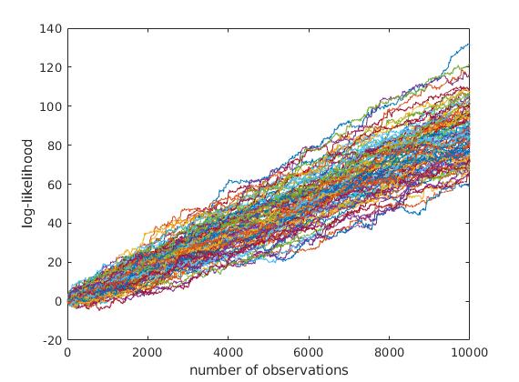
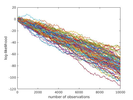
Figure 1: The two images show two log-likelihood plots of sample runs produced by $\pi_{1}$ and $\pi_{2}$, respectively.

By Lemma 2.2.2 it follows that $\ln L_{n}$ converges $\mathbb{P}_{\pi_{1}}$-a.s. (almost-surely) to $\infty$ and $\mathbb{P}_{\pi_{2}}$-a.s. to $-\infty$. This is affirmed by Figure 1. Both log-likelihood plots also appear to follow a particular slope. This suggests that we can distinguish between words produced by $\pi_{1}$ and $\pi_{2}$ by tracking the value of $\ln L_{n}$ to see whether it crosses a lower or upper threshold. This is the intuition behind the Sequential Probability Ratio Test (SPRT).

3 Sequential Probability Ratio Test

Fix an HMM $H=(Q,\Sigma,\Psi)$ for the rest of the paper. Given initial distributions $\pi_{1},\pi_{2}$ and error bounds $\alpha,\beta\in(0,1)$, the SPRT runs as follows. It continues to read observations and computes the value of $\ln L_{n}$ until $\ln L_{n}$ leaves the interval $[A,B]$, where $A:=\ln\frac{\alpha}{1-\beta}$ and $B:=\ln\frac{1-\alpha}{\beta}$. If $\ln L_{n}\leq A$ the test outputs “$\pi_{2}$” and if $\ln L_{n}\geq B$ the test outputs “$\pi_{1}$”. We may view the SPRT as a random variable $\mathrm{SPRT}_{\alpha,\beta}:\Sigma^{\omega}\rightarrow\{\pi_{1},\pi_{2},?\}$, where $?$ denotes that the SPRT does not terminate, i.e., $\ln L_{n}\in[A,B]$ for all $n$. We have the following correctness property.

Proposition 3.1.

Suppose $\pi_{1}$ and $\pi_{2}$ are distinguishable. Let $\alpha,\beta\in(0,1)$. By choosing $A=\ln\frac{\alpha}{1-\beta}$ and $B=\ln\frac{1-\alpha}{\beta}$, we have $\mathbb{P}_{\pi_{1}}(\mathrm{SPRT}_{\alpha,\beta}=\pi_{2})\leq\alpha$ and $\mathbb{P}_{\pi_{2}}(\mathrm{SPRT}_{\alpha,\beta}=\pi_{1})\leq\beta$.

In the following we consider the SPRT with respect to the measure $\mathbb{P}_{\pi_{2}}$. This is without loss of generality as there is a dual version of the $\mathrm{SPRT}$, say $\overline{\mathrm{SPRT}}$ with $\overline{L}_{n}=1/L_{n}$ instead of $L_{n}$, such that $\overline{\mathrm{SPRT}}_{\beta,\alpha}=\mathrm{SPRT}_{\alpha,\beta}$. Define the stopping time

$$N_{\alpha,\beta}\ :=\ \min\{n\in\mathbb{N}\mid\ln L_{n}\not\in[A,B]\}\ \in\ \mathbb{N}\cup\{\infty\}\,.$$

We have that $N_{\alpha,\beta}$ is monotone decreasing in the sense that for $\alpha\leq\alpha^{\prime}$ and $\beta\leq\beta^{\prime}$ we have $N_{\alpha,\beta}\geq N_{\alpha^{\prime},\beta^{\prime}}$. When $\pi_{1}$ and $\pi_{2}$ are distinguishable, $N_{\alpha,\beta}$ is $\mathbb{P}_{\pi_{2}}$-a.s. finite by Lemma 2.2.2.

3.1 Expectation of $N_{\alpha,\beta}$

Consider the two-state HMM where $p_{1}\neq p_{2}$.

(The Dirac distributions of) $s_{1}$ and $s_{2}$ are distinguishable. Further, the increments $\ln L_{n+1}-\ln L_{n}$ are independent and identically distributed (i.i.d.) and $0>\mathbb{E}_{s_{2}}[\ln L_{n+1}-\ln L_{n}]=p_{2}\ln\frac{p_{1}}{p_{2}}+(1-p_{2})\ln\frac{1-p_{1}}{1-p_{2}}=:\ell$. Intuitively as $\ell$ gets more negative, the HMMs become more different. Indeed, Wald [37] shows that the expected stopping time $\mathbb{E}_{s_{2}}[N_{\alpha,\beta}]$ and $\ell$ are inversely proportional:

$$\mathbb{E}_{s_{2}}[N_{\alpha,\beta}]=\frac{\beta\ln\frac{1-\alpha}{\beta}+(1-\beta)\ln\frac{\alpha}{1-\beta}}{\ell}.$$ (1)

This Wald formula cannot hold in general for (multi-state) HMMs. The increments $\ln L_{n+1}-\ln L_{n}$ need not be independent and $\mathbb{E}_{s_{2}}[\ln L_{n+1}-\ln L_{n}]$ can be different for different $n$. Further, $|\ln L_{n+1}-\ln L_{n}|$ can be unbounded; cf. [24, Example 6].

Nevertheless, in Figure 1 we observed that $\ln L_{n}$ appears to decrease linearly (on the $\pi_{2}$ plot). Indeed, we show in Theorem 3.5 below that the limit $\lim_{n\rightarrow\infty}\frac{1}{n}\ln L_{n}$ exists $\mathbb{P}_{\pi_{2}}$-almost surely. Intuitively it corresponds to the average slope of the log-likelihood plot for $\pi_{2}$. In the two-state case, there is a simple proof of this using the law of large numbers:

$$\lim_{n\rightarrow\infty}\frac{1}{n}\ln L_{n}=\lim_{n\rightarrow\infty}\frac{1}{n}\sum_{i=0}^{n-1}[\ln L_{i+1}-\ln L_{i}]=\mathbb{E}_{\pi_{2}}[\ln L_{1}-\ln L_{0}]=\ell\ \ \mathbb{P}_{\pi_{2}}\text{-a.s.}$$

The number $\ell$ is called a likelihood exponent, as defined generally in the following definition.

Definition 3.2.

For initial distributions $\pi_{1},\pi_{2}$, a number $\ell\in[-\infty,0]$ is a likelihood exponent if $\mathbb{P}_{\pi_{2}}(\lim_{n\rightarrow\infty}\frac{1}{n}\ln L_{n}=\ell)>0$.

By Lemma 2.2.1 we have $\mathbb{P}_{\pi_{2}}(\lim_{n\rightarrow\infty}\frac{1}{n}\ln L_{n}>0)=0$, as $\mathbb{P}_{\pi_{2}}(\lim_{n\rightarrow\infty}L_{n}<\infty)=1$. Hence, we may restrict likelihood exponents to $[-\infty,0]$. We write $\Lambda_{\pi_{1},\pi_{2}}\subseteq[-\infty,0]$ for the set of likelihood exponents for $\pi_{1},\pi_{2}$ and define $\Lambda:=\bigcup_{\pi_{1},\pi_{2}}\Lambda_{\pi_{1},\pi_{2}}$; i.e., $\Lambda$ depends only on the HMM $\mathcal{H}$. For $\ell\in\Lambda$ we define the event $E_{\ell}=\{\lim_{n\rightarrow\infty}\frac{1}{n}\ln L_{n}=\ell\}$.

Example 3.3.

In the case of Example 2.3 we have $\Lambda_{\pi_{1},\pi_{2}}=\{\ell\}$ where the slope of the right hand side of Figure 1 suggests that $\ell\approx-\frac{80}{10000}=-0.008$.

Example 3.4.

Even for fixed $\pi_{1},\pi_{2}$ there may be multiple likelihood exponents. Consider the following HMM with initial Dirac distributions $\pi_{1}=e_{s_{1}}$ and $\pi_{2}=e_{s_{4}}$.

We observe two different likelihood exponents depending on the first letter produced. If the first letter is $a$ then $\ln L_{n+1}-\ln L_{n}$ are i.i.d. for $n\geq 1$ and $\lim_{n\rightarrow\infty}\frac{1}{n}\ln L_{n}=\frac{1}{2}\ln\frac{1/3}{1/2}+\frac{1}{2}\ln\frac{2/3}{1/2}=\frac{1}{2}\ln\frac{8}{9}=:\ell$ like the two-state example above. If the first letter is $b$ then $L_{n}=\frac{3}{2}$ for all $n\geq 1$ and $\lim_{n\rightarrow\infty}\frac{1}{n}\ln L_{n}=0$. Thus, $\Lambda_{\pi_{1},\pi_{2}}=\{\ell,0\}$ and $\mathbb{P}_{\pi_{2}}(E_{\ell})=\mathbb{P}_{\pi_{2}}(E_{0})=\frac{1}{2}$.

The following theorem is perhaps the most fundamental contribution of this paper.

Theorem 3.5.

For any initial distributions $\pi_{1},\pi_{2}$ the limit $\lim_{n\rightarrow\infty}\frac{1}{n}\ln L_{n}$ exists $\mathbb{P}_{\pi_{2}}$-almost surely. Furthermore, we have $|\Lambda|\leq|Q|^{2}+1$.

It follows from a stronger theorem, Theorem 5.3, which we prove in Section 5.

Returning to the SPRT, we investigate how $\lim_{n\rightarrow\infty}\frac{1}{n}\ln L_{n}$ influences the performance of the SPRT for small $\alpha$ and $\beta$. Intuitively we expect a steeper slope in the likelihood plot (cf. Figure 1) to lead to faster termination. In the two-state case, Wald’s formula (1) becomes

$$\mathbb{E}_{s_{2}}[N_{\alpha,\beta}]=\frac{\beta\ln\frac{1-\alpha}{\beta}+(1-\beta)\ln\frac{\alpha}{1-\beta}}{\ell}\sim\frac{\ln\alpha}{\ell}\ (\text{as }\alpha,\beta\rightarrow 0),$$ (2)

where we use the notation $\sim$ defined as follows. For functions $f,g:(0,\infty)\times(0,\infty)\to(0,\infty)$ we write “$f(x,y)\sim g(x,y)$ (as $x,y\to 0$)” to denote that for all $\varepsilon>0$ there is $\delta>0$ such that for all $x,y\in(0,\delta)$ we have $f(x,y)/g(x,y)=[1-\varepsilon,1+\varepsilon]$.

In Theorem 3.6 below we generalise Equation 2 to arbitrary HMMs. Indeed a very similar asymptotic identity holds. In the case that $\Lambda=\{\ell\}$ and $\ell\in(-\infty,0)$ we have $\mathbb{E}_{s_{2}}[N_{\alpha,\beta}]\sim\frac{\ln\alpha}{\ell}$ as $\alpha,\beta\rightarrow 0$. If $|\Lambda|>1$ then we condition our expectation on $\lim_{n\rightarrow\infty}\frac{1}{n}\ln L_{n}$.

Theorem 3.6 (Generalised Wald Formula).

Let $\ell$ be a likelihood exponent and let $\pi_{1}$ and $\pi_{2}$ be initial distributions.

1. If $\ell\in(-\infty,0)$ then $\displaystyle\mathbb{E}_{\pi_{2}}\big{[}N_{\alpha,\beta}\mid E_{\ell}\big{]}\sim\frac{\ln\alpha}{\ell}\ \ (\text{as }\alpha,\beta\rightarrow 0)$.

2. If $\ell=0$ then there exist $\alpha,\beta>0$ such that $\displaystyle\mathbb{E}_{\pi_{2}}\big{[}N_{\alpha,\beta}\mid E_{\ell}\big{]}=\infty$.

3. If $\ell=-\infty$ then $\displaystyle\sup_{\alpha,\beta}\leavevmode\nobreak\ \mathbb{E}_{\pi_{2}}\big{[}N_{\alpha,\beta}\mid E_{\ell}\big{]}<\infty$.

The theorem above pertains to the expectation of $N_{\alpha,\beta}$. In the next subsection we give additional information about the distribution of $N_{\alpha,\beta}$, further strengthening the connection between $N_{\alpha,\beta}$ and likelihood exponents.

3.2 Distribution of $N_{\alpha,\beta}$

3.2.1 Likelihood Exponent $0$

Example 3.7.

We continue with Example 3.4 to illustrate the second case in Theorem 3.6. By picking $\alpha=\frac{1}{4},\beta=\frac{1}{4}$ the thresholds for the SPRT are $A=\ln\frac{1}{3}$ and $B=\ln 3$. If the first letter is $b$, then $\ln L_{n}=\ln\frac{3}{2}$ for all $n>1$, thus never crosses the SPRT bounds and $\lim_{n\rightarrow\infty}\frac{1}{n}\ln L_{n}=0$. Hence with probability $\frac{1}{2}$ the SPRT fails to terminate and $N_{\alpha,\beta}=\infty$. It follows that $\mathbb{P}_{\pi_{2}}(E_{0})=\frac{1}{2}$ and $\mathbb{E}_{\pi_{2}}[N_{\alpha,\beta}\mid E_{0}]=\infty$ and, thus, $\mathbb{E}_{\pi_{2}}[N_{\alpha,\beta}]=\infty$.

The second part of Theorem 3.6 says that the expectation of $N_{\alpha,\beta}$ conditioned under $E_{0}$ is infinite. The following proposition strengthens this statement. Conditioning under $E_{0}$, the probability that $N_{\alpha,\beta}$ is infinite converges to $1$ as $\alpha,\beta\rightarrow 0$. Recall that $N_{\alpha,\beta}$ is monotone decreasing. It follows that $\{N_{\alpha^{\prime},\beta^{\prime}}=\infty\}\subseteq\{N_{\alpha,\beta}=\infty\}$ if $\alpha\leq\alpha^{\prime}$ and $\beta\leq\beta^{\prime}$.

Proposition 3.8.

The following two equalities hold up to $\mathbb{P}_{\pi_{2}}$-null sets:

$$E_{0}\leavevmode\nobreak\ =\leavevmode\nobreak\ \left\{\lim_{n\rightarrow\infty}L_{n}>0\right\}\leavevmode\nobreak\ =\leavevmode\nobreak\ \bigcup_{\alpha,\beta>0}\left\{N_{\alpha,\beta}=\infty\right\}.$$

Thus, $\lim_{\alpha,\beta\rightarrow 0}\mathbb{P}_{\pi_{2}}(N_{\alpha,\beta}=\infty)=\mathbb{P}_{\pi_{2}}(E_{0})$.

Corollary 3.9 (using Lemma 2.2.2).

Initial distributions $\pi_{1}$ and $\pi_{2}$ are distinguishable if and only if $\mathbb{P}_{\pi_{2}}(E_{0})=0$ if and only if $\mathbb{P}_{\pi_{2}}(N_{\alpha,\beta}<\infty)=1$ holds for all $\alpha,\beta>0$.

3.2.2 Likelihood Exponent $-\infty$

Example 3.10.

Consider now a modification of Example 3.4 where state $s_{3}$ has the $b$ loop removed.

The likelihood exponents are $-\infty$ and $\ell:=\frac{1}{2}\ln\frac{8}{9}$ so that $\Lambda=\{-\infty,\ell\}$. Also, $\mathbb{P}_{s_{4}}(E_{-\infty})=\mathbb{P}_{s_{4}}(E_{\ell})=\frac{1}{2}$. Up to $\mathbb{P}_{s_{4}}$-null sets the events $E_{-\infty}$, $b\Sigma^{\omega}$ and $ba^{*}b\Sigma^{\omega}$ are equal. The event $ba^{*}b\Sigma^{\omega}$ represents the right chain producing an observation which the left chain cannot produce, causing the SPRT to terminate for any $\alpha,\beta$. Therefore conditioned on $E_{-\infty}$, the random variable $N_{\alpha,\beta}-1$ is bounded by a geometric random variable with parameter $\frac{1}{2}$. Hence $\sup_{\alpha,\beta}\mathbb{E}_{\pi_{2}}\leavevmode\nobreak\ \Big{[}N_{\alpha,\beta}\mid E_{-\infty}\Big{]}\leq 1+2$.

We define the stopping time $N_{\perp}=\min\{n\in\mathbb{N}\mid L_{n}=0\}$. Note that $\sup_{\alpha,\beta}N_{\alpha,\beta}\leq N_{\perp}$ since $\{L_{n}=0\}\subseteq\{L_{n}\leq\frac{\alpha}{1-\beta}\}$ for all $\alpha,\beta$. By the following proposition, the reverse inequality also holds.

Proposition 3.11.

The events $E_{-\infty}$ and $\{L_{n}=0\text{ for some }n\}$ are equal. Thus, $\sup_{\alpha,\beta}N_{\alpha,\beta}=N_{\perp}$ and $\lim_{\alpha,\beta\rightarrow 0}\mathbb{P}_{\pi_{2}}(N_{\alpha,\beta}<\infty)=\mathbb{P}_{\pi_{2}}(E_{-\infty})$.

Applying this to Example 3.10, we obtain $\sup_{\alpha,\beta}\mathbb{E}_{\pi_{2}}\big{[}N_{\alpha,\beta}\mid E_{-\infty}\big{]}=3$.

3.2.3 Likelihood Exponent in $(-\infty,0)$

Conditioned on $E_{\ell}$ where $\ell\in(-\infty,0)$, Theorem 3.6 states that $N_{\alpha,\beta}$ scales with $\frac{\ln\alpha}{\ell}$ in expectation. The following result shows that this relationship also holds $\mathbb{P}_{\pi_{2}}$-almost surely.

Proposition 3.12.

Let $\ell\in\Lambda$ and assume $\ell\in(-\infty,0)$. We have

$$\mathbb{P}_{\pi_{2}}\Big{(}N_{\alpha,\beta}\sim\frac{\ln\alpha}{\ell}\ \ (\text{as }\alpha,\beta\rightarrow 0)\;\Big{|}\;E_{\ell}\Big{)}\leavevmode\nobreak\ =\leavevmode\nobreak\ 1.$$

In fact, we prove the first part of Theorem 3.6 using Proposition 3.12. If there were a bound $M\in\mathbb{N}$ such that $\mathbb{P}_{\pi_{2}}$-a.s. $\frac{N_{\alpha,\beta}}{-\ln\alpha}\leq M$, the first part of Theorem 3.6 would follow from Proposition 3.12 by the dominated convergence theorem. However this is not the case in general. Instead we show in Section B.4 that the set of random variables $\{\frac{N_{\alpha,\beta}}{-\ln\alpha}\mid 0<\alpha,\beta\leq\frac{1}{2}\}$ is uniformly integrable with respect to the measure $\mathbb{P}_{\pi_{2}}$ and then use Vitali’s convergence theorem.

Example 3.13.

Recall Example 2.3, where $\Lambda=\{\ell\}$.

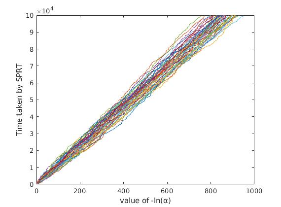
Figure 2: The time taken by the SPRT for $0\leq-\ln\alpha=-\ln\beta\leq 1000$.

Figure 2 demonstrates the asymptotic relationship in Proposition 3.12. Each of the $50$ lines correspond to a sample run and we record the value of $N_{\alpha,\beta}$ for $0\leq-\ln\alpha=-\ln\beta\leq 1000$. From the figure we estimate $-\frac{1}{\ell}$ as $\frac{10^{5}}{800}=125$. This coincides with the estimate given in Example 3.3.

We conclude from this section that the performance of the SPRT, in terms of its termination time $N_{\alpha,\beta}$, is tightly connected to likelihood exponents. This motivates our study of likelihood exponents in the rest of the paper.

4 Probability of $E_{\ell}$

In this section we aim at computing $\mathbb{P}_{\pi_{2}}(E_{\ell})$ for a likelihood exponent $\ell$. We show the following theorem.

Theorem 4.1.

Given an HMM and initial distributions $\pi_{1},\pi_{2}$,

1. one can compute $\mathbb{P}_{\pi_{2}}(\lim_{n\rightarrow\infty}\frac{1}{n}\ln L_{n}=-\infty)$ and $\mathbb{P}_{\pi_{2}}(\lim_{n\rightarrow\infty}\frac{1}{n}\ln L_{n}=0)$ in PSPACE;

2. one can decide whether $\mathbb{P}_{\pi_{2}}(\lim_{n\rightarrow\infty}\frac{1}{n}\ln L_{n}=0)=0$ (i.e., $0\not\in\Lambda_{\pi_{1},\pi_{2}}$) in polynomial time;

3. deciding whether $\mathbb{P}_{\pi_{2}}(\lim_{n\rightarrow\infty}\frac{1}{n}\ln L_{n}=0)=1$, whether $\mathbb{P}_{\pi_{2}}(\lim_{n\rightarrow\infty}\frac{1}{n}\ln L_{n}=-\infty)=0$, and whether $\mathbb{P}_{\pi_{2}}(\lim_{n\rightarrow\infty}\frac{1}{n}\ln L_{n}=-\infty)=1$ are all PSPACE-complete problems.

The following example illustrates the construction underlying the PSPACE upper bound.

Example 4.2.

Consider another adaption of Example 3.4.

If the first letter produced by $s_{4}$ is $b$, then $L_{n}=\frac{3}{2}$ for all $n\in\mathbb{N}$. If the first two letters are $ab$, then $L_{1}=\frac{1}{2}$ and $L_{n}=0$ for $n\geq 2$. If the first two letters are $aa$, then $s_{5}\in\mathrm{supp}(e_{s_{1}}\Psi(aaw))$ for all $w\in\Sigma^{*}$, and therefore, up to a $\mathbb{P}_{s_{4}}$-null set, $L_{n}>0$ holds for all $n\in\mathbb{N}$, which implies (using Proposition 3.11) that there is $\ell\in(-\infty,0)$ such that $\lim_{n\rightarrow\infty}\frac{1}{n}\ln L_{n}=\ell$. Thus, $\Lambda_{s_{1},s_{4}}=\{-\infty,\ell,0\}$.

The likelihood ratio $L_{n}$ is $0$ if and only if $\mathrm{supp}(\pi_{1}\Psi(w_{n}))=\emptyset$. In order to track the support of $\pi_{1}\Psi(w_{n})$, we consider the left part of the HMM as an NFA with $s_{1}$ as the initial state and its determinisation as shown in the DFA below.

Almost surely, $s_{4}$ produces a word that drives this DFA into a bottom SCC, which then determines $\lim_{n\rightarrow\infty}\frac{1}{n}\ln L_{n}$: concretely, the bottom SCC $\{\{s_{5}\},\{s_{2},s_{5}\}\}$ is associated with $\ell$, the bottom SCC $\{\emptyset\}$ with $-\infty$, and the bottom SCC $\{\{s_{3}\}\}$ with $0$.

In general, the observations need not be produced uniformly at random but by an HMM. Therefore, in the following construction, we also keep track of the “current” state of the HMM which produces the observations. For $S\subseteq Q$ and $a\in\Sigma$, define $\delta(S,a):=\{q^{\prime}\in Q\mid\exists\,q\in S:\Psi(a)_{q,q^{\prime}}>0\}$. Define the Markov chain $\mathcal{B}:=(2^{Q}\times Q,T)$ where

$$T_{(S,q),(S^{\prime},q^{\prime})}\ :=\ \sum_{\delta(S,a)=S^{\prime}}\Psi(a)_{q,q^{\prime}}\,.$$

Given initial distributions $\pi_{1},\pi_{2}$ on $Q$ as before, define an initial distribution $\iota$ on $2^{Q}\times Q$ by $\iota((\mathrm{supp}(\pi_{1}),q)):=(\pi_{2})_{q}$. Intuitively, the left part $S$ of a state $(S,q)$ tracks the support of $\pi_{1}\Psi(w_{n})$, and the right part $q$ tracks the current state of the HMM that had been initialised at a random state from $\pi_{2}$. The following lemma states the key properties of this construction.

Lemma 4.3.

Consider the Markov chain $\mathcal{B}=(2^{Q}\times Q,T)$ defined above.

1. Every bottom SCC of $\mathcal{B}$ is associated with a single likelihood exponent; i.e., for every bottom SCC $C\subseteq 2^{Q}\times Q$ there is $\ell(C)\in[-\infty,0]$ such that for any initial distribution $\pi_{1}\in[0,1]^{Q}$ and any state $q_{2}\in Q$ with $(\mathrm{supp}(\pi_{1}),q_{2})\in C$ we have $\Lambda_{\pi_{1},e_{q_{2}}}=\{\ell(C)\}$.

2. Let $(S,q)\in C$ for a bottom SCC $C$. If $S=\emptyset$ then $\ell(C)=-\infty$; otherwise, if $e_{q}$ and the uniform distribution on $S$ are not distinguishable then $\ell(C)=0$; otherwise $\ell(C)\in(-\infty,0)$.

3. We have $\mathbb{P}_{\pi_{2}}(E_{\ell})=\mathbb{P}_{\iota}(\{\text{visit bottom SCC $C$ with $\ell(C)=\ell$}\})$.

All parts of the lemma rely on the observation that $\lim_{n\rightarrow\infty}\frac{1}{n}\ln L_{n}$ depend only on the support of $\pi_{1}$ and on the support of $\pi_{2}$. The first part of the lemma follows from Lévy’s 0-1 law. We use this lemma for the proof of Theorem 4.1.1.

Proof 4.4 (Proof sketch for Theorem 4.1.1).

The Markov chain $\mathcal{B}$ from Lemma 4.3 is exponentially big but can be constructed by a PSPACE transducer, i.e., a Turing machine whose work tape (but not necessarily its output tape) is PSPACE-bounded. This PSPACE transducer can also identify the bottom SCCs. For each bottom SCC $C$, the PSPACE transducer also decides whether $\ell(C)=-\infty$ or $\ell(C)\in(-\infty,0)$ or $\ell(C)=0$, using Lemma 4.3.2 and the polynomial-time algorithm for distinguishability from [10]. Finally, to compute $\mathbb{P}_{\pi_{2}}(E_{-\infty})$ and $\mathbb{P}_{\pi_{2}}(E_{0})$, by Lemma 4.3.3, it suffices to set up and solve a linear system of equations for computing hitting probabilities in a Markov chain. This system can also be computed by a PSPACE transducer. Since linear systems of equations can be solved in the complexity class NC, which is included in polylogarithmic space, one can use standard techniques for composing space-bounded transducers to compute $\mathbb{P}_{\pi_{2}}(E_{-\infty})$ and $\mathbb{P}_{\pi_{2}}(E_{0})$ in PSPACE.

Proof 4.5 (Proof of Theorem 4.1.2).

Immediate from Corollary 3.9 and the polynomial-time decidability of distinguishability [10].

Towards a proof of Theorem 4.1.3, we use the mortality problem, which asks, given a finite set of states $Q$, a finite alphabet $\Sigma$, and a function $\Phi:\Sigma\to\{0,1\}^{Q\times Q}$, whether there exists a word $w\in\Sigma^{*}$ such that $\Phi(w)$ is the zero matrix. The mortality problem can be viewed as a special case of the NFA non-universality problem (given an NFA, does it reject some word?). Like NFA universality, the mortality problem is PSPACE-complete [22].

Concerning $\mathbb{P}_{\pi_{2}}(E_{-\infty})$ (cf. Theorem 4.1.3), we actually show a stronger result, namely that any nontrivial approximation of $\mathbb{P}_{\pi_{2}}(E_{-\infty})$ is PSPACE-hard. The proof is also based on the mortality problem.

Proposition 4.6.

There is a polynomial-time computable function that maps any instance of the mortality problem to an HMM and initial distributions $\pi_{1},\pi_{2}$ so that if the instance is positive then $\mathbb{P}_{\pi_{2}}(E_{-\infty})=1$ and if the instance is negative then $\mathbb{P}_{\pi_{2}}(E_{-\infty})=0$. Thus, any nontrivial approximation of $\mathbb{P}_{\pi_{2}}(E_{-\infty})$ is PSPACE-hard.

Proof 4.7.

Let $(Q,\Sigma,\Phi)$ be an instance of the mortality problem. If there is $q\in Q$ that indexes a zero row in $\sum_{a\in\Sigma}\Phi(a)$, remove the row and column indexed by $q$ in all $\Phi(a)$. Thus, we can assume without loss of generality that $\sum_{a\in\Sigma}\Phi(a)$ has no zero row. Construct an HMM $(Q,\Sigma,\Psi)$ so that $\Phi(a)$ and $\Psi(a)$ have the same zero pattern for all $a\in\Sigma$. Define $\pi_{1}$ as a uniform distribution on $Q$. Define $\pi_{2}$ as a Dirac distribution on a fresh state that emits letters from $\Sigma$ uniformly at random. Thus, if $(Q,\Sigma,\Phi)$ is a positive instance of the mortality problem then $\mathbb{P}_{\pi_{2}}(E_{-\infty})=1$, and if $(Q,\Sigma,\Phi)$ is a negative instance then $\mathbb{P}_{\pi_{2}}(E_{-\infty})=0$.

The proof that deciding whether $\mathbb{P}_{\pi_{2}}(E_{0})=1$ is PSPACE-hard is similarly based on mortality.

5 Representing Likelihood Exponents

In the following we show that one can efficiently represent likelihood exponents in terms of Lyapunov exponents. The definition of Lyapunov exponents is based on the following definition.

Definition 5.1.

A matrix system is a triple $\mathcal{M}=(Q,\Sigma,\Psi)$ where $Q$ is a finite set of states, $\Sigma$ is a finite set of observations, and $\Psi:\Sigma\to\mathbb{R}_{\geq 0}^{Q\times Q}$ specifies the transitions. (Note that an HMM is a matrix system.) A Lyapunov system is a pair $\mathcal{S}=(\mathcal{M},\rho)$ where $\mathcal{M}=(Q,\Sigma,\Psi)$ is a matrix system and $\rho\in(0,1]^{\Sigma}$ is a probability distribution with full support, such that the directed graph $(Q,E)$ with $E=\{(q,r)\mid\sum_{a\in\Sigma}\Psi_{q,r}(a)>0\}$ is strongly connected.

We can identify the probability distribution $\rho$ from this definition with the single-state HMM $(\{s\},\Sigma,\Psi_{\rho})$ where $\Psi_{\rho}(a)_{s,s}=\rho(a)$ for all $a\in\Sigma$. In this way, $\rho$ produces a random infinite word from $\Sigma^{\omega}$. We will write $\mathbb{P}_{\rho}$ for the associated probability measure. The following lemma is Theorem 1 from [30].

Lemma 5.2 ([30]).

Let $((Q,\Sigma,\Psi),\rho)$ be a Lyapunov system. Then there is $\lambda\in\mathbb{R}$ such that, for all $\pi\in[0,\infty)^{Q}$, $\mathbb{P}_{\rho}$-a.s., either $\pi\Psi(w_{n})=\vec{0}$ for some $n\in\mathbb{N}$ or the limit $\lim_{n\to\infty}\frac{1}{n}\ln\|\pi\Psi(w_{n})\|$ exists and equals $\lambda$.

For a Lyapunov system $\mathcal{S}$ we call $\lambda(\mathcal{S})=\lambda$ from the lemma the Lyapunov exponent defined by $\mathcal{S}$. We prove the following theorem, which implies Theorem 3.5.

Theorem 5.3.

Given an HMM $(Q,\Sigma,\Psi)$ we can compute in polynomial time $2K\leq 2|Q|^{2}$ Lyapunov systems $\mathcal{S}_{1}^{1},\mathcal{S}_{1}^{2},\mathcal{S}_{2}^{1},\mathcal{S}_{2}^{2},\ldots,\mathcal{S}_{K}^{1},\mathcal{S}_{K}^{2}$ such that for any initial distributions $\pi_{1},\pi_{2}$ the limit $\lim_{n\rightarrow\infty}\frac{1}{n}\ln L_{n}$ exists $\mathbb{P}_{\pi_{2}}$-a.s. and lies in

$$\Lambda\ \subseteq\ \{-\infty\}\cup\{\lambda(\mathcal{S}_{1}^{1})-\lambda(\mathcal{S}_{1}^{2}),\ldots,\lambda(\mathcal{S}_{K}^{1})-\lambda(\mathcal{S}_{K}^{2})\}\,.$$

In particular, the HMM $(Q,\Sigma,\Psi)$ has at most $|Q|^{2}+1$ likelihood exponents.

In the rest of the section we provide more details on the construction underlying Theorem 5.3. As an intermediate concept (between the given HMM and the Lyapunov systems from Theorem 5.3) we define generalized Lyapunov systems.

Lemma 5.4.

Let $\mathcal{S}=((Q_{1},\Sigma,\Psi_{1}),(Q_{2},\Sigma,\Psi_{2}),C)$ be a generalized Lyapunov system.

1. There is $\lambda\in\mathbb{R}$, henceforth called $\lambda(\mathcal{S})$, such that, for all $\pi_{1}\in[0,\infty)^{Q_{1}}$ and all probability distributions $\pi_{2}\in[0,1]^{Q_{2}}$ with $\mathrm{supp}(\pi_{1})\times\mathrm{supp}(\pi_{2})\subseteq C$, we have $\mathbb{P}_{\pi_{2}}$-a.s. that either $\pi_{1}\Psi_{1}(w_{n})=\vec{0}$ for some $n\in\mathbb{N}$ or the limit $\lim_{n\to\infty}\frac{1}{n}\ln\|\pi_{1}\Psi_{1}(w_{n})\|$ exists and equals $\lambda(\mathcal{S})$.

2. One can compute in polynomial time a Lyapunov system $\mathcal{S}^{\prime}$ such that $\lambda(\mathcal{S})=\lambda(\mathcal{S}^{\prime})$.

Let $\mathcal{H}=(Q,\Sigma,\Psi)$ be an HMM. Let $R\subseteq Q\times Q$ be a (not necessarily bottom) SCC of the graph $G_{\mathcal{H},\mathcal{H}}$ such that $Q_{R}:=\{q_{2}\in Q\mid\exists\,q_{1}\in Q:(q_{1},q_{2})\in R\}$ is a bottom SCC of the graph of $\sum_{a\in\Sigma}\Psi(a)$. We call such $R$ a right-bottom SCC. Clearly there are at most $|Q|^{2}$ right-bottom SCCs. Towards Theorem 5.3 we want to define, for each right-bottom SCC $R$, two generalized Lyapunov systems $\mathcal{S}_{R}^{1},\mathcal{S}_{R}^{2}$. Intuitively, $\mathcal{S}_{R}^{1}$ and $\mathcal{S}_{R}^{2}$ correspond to the numerator and the denominator of the likelihood ratio, respectively.

For a function of the form $\Phi:\Sigma\to\mathbb{R}^{Q\times Q}$ and $P\subseteq Q$ we write $\Phi_{|P}:\Sigma\to\mathbb{R}^{P\times P}$ for the function with $\Phi_{|P}(a)(q,r)=\Phi(a)(q,r)$ for all $a\in\Sigma$ and $q,r\in P$; i.e., $\Phi_{|P}(a)$ denotes the principal submatrix obtained from $\Phi(a)$ by restricting it to the rows and columns indexed by $P$.

Define $\Psi^{\prime}(a,r)_{q,r}:=\Psi(a)_{q,r}$ for all $a\in\Sigma$ and $q,r\in Q$. Then $(Q,\Sigma\times Q,\Psi^{\prime})$ is an HMM, which is similar to $\mathcal{H}$, but which emits, in addition to an observation from $\Sigma$, also the next state. Since $Q_{R}$ is a bottom SCC of the graph of $\sum_{a\in\Sigma}\Psi(a)$, the HMM $\mathcal{H}_{2}:=(Q_{R},\Sigma\times Q_{R},\Psi^{\prime}_{|Q_{R}})$ is strongly connected. This HMM $\mathcal{H}_{2}$ will be used both in $\mathcal{S}_{R}^{1}$ and in $\mathcal{S}_{R}^{2}$.

Next, define $\overline{\Psi}:(\Sigma\times Q)\to[0,1]^{(Q\times Q)\times(Q\times Q)}$ by

$$\overline{\Psi}(a,r_{2})_{(q_{1},q_{2}),(r_{1},r_{2})}\ :=\ \Psi(a)_{q_{1},r_{1}}\quad\text{for all }a\in\Sigma\ \text{ and }q_{1},q_{2},r_{1},r_{2}\in Q\,.$$

Now define $\mathcal{S}_{R}^{1}:=(\mathcal{M}^{1},\mathcal{H}_{2},C^{1})$, where $\mathcal{M}^{1}:=(R,\Sigma\times Q_{R},\overline{\Psi}_{|R})$ and $C^{1}:=\{((q_{1},q_{2}),q_{2})\mid(q_{1},q_{2})\in R\}$. Finally, denoting by $R^{\prime}\subseteq Q_{R}\times Q_{R}$ the SCC of the graph $G_{\mathcal{H},\mathcal{H}}$ that contains the “diagonal” vertices $(q,q)\in Q_{R}\times Q_{R}$, define $\mathcal{S}_{R}^{2}:=(\mathcal{M}^{2},\mathcal{H}_{2},C^{2})$, where $\mathcal{M}^{2}:=(R^{\prime},\Sigma\times Q_{R},\overline{\Psi}_{|R^{\prime}})$ and $C^{2}:=\{((q_{1},q_{2}),q_{2})\mid(q_{1},q_{2})\in R^{\prime}\}$.

For sets $U,V\subseteq Q\times Q$ let $U\longrightarrow_{G_{\mathcal{H},\mathcal{H}}}V$ denote that there are $u\in U$ and $v\in V$ such that $v$ is reachable from $u$ in $G_{\mathcal{H},\mathcal{H}}$.

We are ready to state the following key technical lemma:

Lemma 5.5.

Given an HMM $(Q,\Sigma,\Psi)$, let $\mathcal{R}\subseteq 2^{Q\times Q}$ be the set of its right-bottom SCCs, and, for $R\in\mathcal{R}$, let $\mathcal{S}_{R}^{1},\mathcal{S}_{R}^{2}$ be the generalized Lyapunov systems defined above. Then, for any initial distributions $\pi_{1},\pi_{2}$, the limit $\lim_{n\rightarrow\infty}\frac{1}{n}\ln L_{n}$ exists $\mathbb{P}_{\pi_{2}}$-a.s. and lies in

$$\{-\infty\}\cup\{\lambda(\mathcal{S}_{R}^{1})-\lambda(\mathcal{S}_{R}^{2})\mid R\in\mathcal{R},\ \mathrm{supp}(\pi_{1})\times\mathrm{supp}(\pi_{2})\longrightarrow_{G_{\mathcal{H},\mathcal{H}}}R\}\,.$$

Thus, $\Lambda_{\pi_{1},\pi_{2}}\subseteq\{-\infty\}\cup\{\lambda(\mathcal{S}_{R}^{1})-\lambda(\mathcal{S}_{R}^{2})\mid R\in\mathcal{R},\ \mathrm{supp}(\pi_{1})\times\mathrm{supp}(\pi_{2})\longrightarrow_{G_{\mathcal{H},\mathcal{H}}}R\}$.

Proof 5.6 (Proof sketch).

Let $\pi_{1},\pi_{2}$ be initial distributions. Very loosely speaking, we show in the appendix that on $\mathbb{P}_{\pi_{2}}$-almost every run $w$ there is a right-bottom SCC $R$ which “traps” “most” of the mass of $\pi_{1}\Psi(w_{n})$ and $\pi_{2}\Psi(w_{n})$. This can be made meaningful and formal using (the cross-product systems) $\mathcal{S}_{R}^{1},\mathcal{S}_{R}^{2}$. We then show that on $\mathbb{P}_{\pi_{2}}$-almost every such run $w$, for both $i=1,2$, the limit $\lim_{n\to\infty}\frac{1}{n}\ln\|\pi_{i}\Psi(w_{n})\|$ exists and equals $\lambda(\mathcal{S}_{R}^{i})$ (or $\pi_{1}\Psi(w_{n})=\vec{0}$ for some $n$). It follows that

$$\lim_{n\rightarrow\infty}\frac{1}{n}\ln L_{n}\ =\ \lim_{n\to\infty}\frac{1}{n}\ln\frac{\|\pi_{1}\Psi(w_{n})\|}{\|\pi_{2}\Psi(w_{n})\|}\ =\ \lambda(\mathcal{S}_{R}^{1})-\lambda(\mathcal{S}_{R}^{2})\,.$$

With Lemma 5.5 at hand, the proof of Theorem 5.3 is easy:

Proof 5.7 (Proof of Theorem 5.3).

As argued before, the set $\mathcal{R}$ of right-bottom SCCs of the given HMM has at most $|Q|^{2}$ elements. These right-bottom SCCs $R$ and the associated generalized Lyapunov systems $\mathcal{S}_{R}^{1},\mathcal{S}_{R}^{2}$ can be computed in polynomial time. By Lemma 5.5 we have $\Lambda=\bigcup_{\pi_{1},\pi_{2}}\Lambda_{\pi_{1},\pi_{2}}\subseteq\{-\infty\}\cup\{\lambda(\mathcal{S}_{R}^{1})-\lambda(\mathcal{S}_{R}^{2})\mid R\in\mathcal{R}\}$. By Lemma 5.4.2, for each $R\in\mathcal{R}$ one can compute in polynomial time an equivalent Lyapunov system.

Theorem 5.3 allows us to represent the likelihood exponents of an HMM in terms of Lyapunov exponents. In general, approximating or even computing Lyapunov exponents is hard, but there are practical approximation algorithms using convex optimisation [31, 35].

6 Deterministic HMMs

In Sections 4 and 5 we have seen that the problems of representing/computing likelihood exponents and of computing their probabilities tend to be computationally difficult. In this section we study deterministic HMMs and show that this subclass leads to tractable problems. An HMM $(Q,\Sigma,\Psi)$ is deterministic if, for all $a\in\Sigma$, all rows of $\Psi(a)$ contain at most one non-zero entry. Thus, for all $q\in Q$ and $w\in\Sigma^{*}$, we have $|\mathrm{supp}(e_{q}\Psi(w))|\leq 1$.

A useful observation is that the Markov chain $\mathcal{B}=(2^{Q}\times Q,T)$, which was defined before Lemma 4.3 and can be exponential in general, has only quadratic size in the deterministic case if we restrict it to the part that is reachable from initial Dirac distributions.

Example 6.1.

Consider the deterministic HMM $(Q,\Sigma,\Psi)$ in Figure 3(a).

Figure 3: Cross-product constructions for a deterministic HMM.

Let $\pi_{1}=e_{q_{1}}$ and $\pi_{2}=e_{q_{2}}$ (the latter is indicated by an arrow pointing to $q_{2}$). Then the relevant (i.e., reachable from $(\{q_{1}\},q_{2})$) part of $\mathcal{B}$ is shown in Figure 3(b). Let us add back the observations that gave rise to the transitions in $\mathcal{B}$, and for simplicity drop the set brackets in the left component of states. We obtain the HMM in Figure 3(c). With this HMM we may keep track of the exact likelihood ratio. For example, suppose that the word $aba$ is emitted, so that $L_{3}=\frac{\|e_{q_{1}}\Psi(aba)\|}{\|e_{q_{2}}\Psi(aba)\|}=\frac{1}{2}$ and $\mathrm{supp}(e_{q_{1}}\Psi(aba))=\{q_{2}\}$ and $\mathrm{supp}(e_{q_{2}}\Psi(aba))=\{q_{1}\}$. Suppose the next letter is $b$ (which is the case with probability $\frac{1}{3}$). Then $L_{4}$ arises from $L_{3}$ by multiplying with $\frac{\Psi_{q_{2},q_{1}}(b)}{\Psi_{q_{1},q_{2}}(b)}=2$, and the supports are switched again. In terms of log-likelihoods, we have $\ln L_{4}=\ln L_{3}+\ln 2$. This motivates the Markov chain shown in Figure 3(d), where the transitions outgoing from a state $(r_{1},r_{2})$ are labelled by the log-likelihood ratio of their corresponding probabilities in the HMM. The Markov chain has stationary distribution $(\frac{2}{3},\frac{1}{3})$. By the strong ergodic theorem for Markov chains, we obtain (the irrational number)

$$\textstyle\lim_{n\rightarrow\infty}\frac{1}{n}\ln L_{n}\ =\ \frac{2}{3}\Big{(}\frac{2}{3}\ln\frac{1}{2}+\frac{1}{3}\ln 2\Big{)}+\frac{1}{3}\Big{(}\frac{1}{3}\ln 2+\frac{2}{3}\ln\frac{1}{2}\Big{)}\ =\ \frac{1}{3}\ln 2+\frac{2}{3}\ln\frac{1}{2}=-\frac{1}{3}\ln 2\,.$$

In general there may again be several likelihood exponents, including $-\infty$ and $0$. For the rest of the section, let $\mathcal{H}=(Q,\Sigma,\Psi)$ be a deterministic HMM. Motivated by Example 6.1, define an HMM $\mathcal{A}=((Q\times Q)\cup s_{\bot},\hat{\Sigma},\hat{\Psi})$, where $s_{\bot}$ is a fresh state, and

$$\hat{\Sigma}\ :=\ \left\{\ln\frac{\Psi(a)_{q_{1},r_{1}}}{\Psi(a)_{q_{2},r_{2}}}\in[-\infty,\infty)\;\middle|\;a\in\Sigma,\ q_{1},r_{1},q_{2},r_{2}\in Q,\ \Psi(a)_{q_{2},r_{2}}\neq 0\right\}\cup\{-\infty\}$$

$$\hat{\Psi}(\hat{a})_{(q_{1},q_{2}),(r_{1},r_{2})}\ :=\ \sum\left\{\Psi(a)_{q_{2},r_{2}}\;\middle|\;a\in\Sigma:\hat{a}=\ln\frac{\Psi(a)_{q_{1},r_{1}}}{\Psi(a)_{q_{2},r_{2}}}\right\}\quad\text{for }\hat{a}\neq-\infty$$

$$\hat{\Psi}(-\infty)_{(q_{1},q_{2}),s_{\bot}}\ :=\ \sum\left\{\Psi(a)_{q_{2},r_{2}}\;\middle|\;a\in\Sigma,\ r_{2}\in Q:\textstyle\sum_{r_{1}\in Q}\Psi(a)_{q_{1},r_{1}}=0\right\}$$

$$\hat{\Psi}(-\infty)_{s_{\bot},s_{\bot}}\ :=\ 1\,.$$

Note that the embedded Markov chain of $\mathcal{A}$ is similar to the Markov chain $\mathcal{B}$ from Lemma 4.3: states $(\{q_{1}\},q_{2})$ in $\mathcal{B}$ are called $(q_{1},q_{2})$ in $\mathcal{A}$, the states $(\emptyset,q)$ in $\mathcal{B}$ are subsumed by the state $s_{\bot}$ of $\mathcal{A}$, and the states $(S,q)$ in $\mathcal{B}$ with $|S|>1$ are not represented in $\mathcal{A}$. The observations in $\hat{\Sigma}\subseteq[-\infty,\infty)$ track the log-likelihood ratio.

Example 6.2.

Consider the HMM $\mathcal{H}$ on the left, with initial distributions $\pi_{1}=e_{q_{1}}$ and $\pi_{2}=e_{q_{2}}$. The part of $\mathcal{A}$ reachable from $(q_{1},q_{2})$ is shown on the right:

Here we have $\Lambda_{\pi_{1},\pi_{2}}=\{-\infty,0\}$ with $\mathbb{P}_{\pi_{2}}(E_{-\infty})=\mathbb{P}_{\pi_{2}}(E_{0})=\frac{1}{2}$.

Denote by $\bar{\mathcal{A}}$ the embedded Markov chain of $\mathcal{A}$. Let $C\subseteq Q\times Q$ be a non-$\{s_{\bot}\}$ bottom SCC of $\bar{\mathcal{A}}$. Let $\mu\in[0,1]^{C}$ denote the stationary distribution of the restriction of $\bar{\mathcal{A}}$ on $C$. Define the vector $\nu\in\mathbb{R}^{C}$ of average observations by $\nu_{(r_{1},r_{2})}\ :=\ \sum_{\hat{a}\in\hat{\Sigma}}\|e_{(r_{1},r_{2})}\hat{\Psi}(\hat{a})\|\cdot\hat{a}$. By the strong ergodic theorem for Markov chains, the average observation in $C$ equals $\mu\nu^{\top}=:\ell(C)$. Extend this definition by $\ell(\{s_{\bot}\}):=-\infty$. Then we have the following lemma.

Lemma 6.3.

Let $\pi_{1}=e_{q_{1}}$ and $\pi_{2}=e_{q_{2}}$ be initial distributions. For the Markov chain $\bar{\mathcal{A}}$ define $\iota:=e_{(q_{1},q_{2})}$. We have $\mathbb{P}_{\pi_{2}}(E_{\ell})=\mathbb{P}_{\iota}(\{\text{visit bottom SCC $C$ with $\ell(C)=\ell$}\})$.

The proof is essentially the same as in Lemma 4.3.3. This gives us the following result.

Theorem 6.4.

Given a deterministic HMM $(Q,\Sigma,\Psi)$ with initial Dirac distributions $\pi_{1},\pi_{2}$, one can compute in polynomial time

1. $\Lambda_{\pi_{1},\pi_{2}}$ as a set of expressions of the form $\sum_{i}x_{i}\ln y_{i}$ where $x_{i},y_{i}\in\mathbb{Q}$, and

2. $\Pr_{\pi_{2}}(E_{\ell})$ for each such $\ell\in\Lambda_{\pi_{1},\pi_{2}}$.

Proof 6.5 (Proof sketch).

The theorem follows mostly from Lemma 6.3, with the slight complication that for part 2 we have to check numbers of the form $\sum_{i}x_{i}\ln y_{i}$ (where $x_{i},y_{i}\in\mathbb{Q}$) for equality. But this can be done in polynomial time as shown in [17].

7 Conclusions

We have shown that the performance of the SPRT is tightly connected with likelihood exponents. These numbers are related to Lyapunov exponents and can be viewed as a distance measure between HMMs. We have shown that the number of likelihood exponents is quadratic in the number of states. The associated computational problems tend to be complex (PSPACE-hard), but become tractable for deterministic HMMs. In our work we did not make any ergodicity assumptions on the HMMs, unlike in earlier works from mathematics and engineering such as [21, 8, 18, 20]. Efficient approximation of likelihood exponents, in theory or praxis, remains an open problem.

Appendix A Proofs and Additional Material on Section 2

A.1 Proof of Lemma 2.2

See 2.2

Proof A.1.

The first part is [10, Proposition 6]. Towards the second part, the following equalities hold.

$$1-d(\pi_{1},\pi_{2}) =\lim_{n\rightarrow\infty}\sum_{w\in\Sigma^{n}}\min\{\|\pi_{1}\Psi(w)\|,\|\pi_{2}\Psi(w)\|\}$$ by [10, Theorem  7]

$$=\lim_{n\rightarrow\infty}\sum_{w\in\Sigma^{n}}\min\{L_{n}(w),1\}\|\pi_{2}\Psi(w)\|$$

$$=\lim_{n\rightarrow\infty}\mathbb{E}_{\pi_{2}}\big{[}\min\{L_{n},1\}\big{]}$$

$$=\mathbb{E}_{\pi_{2}}\big{[}\lim_{n\rightarrow\infty}\min\{L_{n},1\}\big{]} \text{as }0\leq\min\{L_{n}(w),1\}\leq 1.$$

Then, $\lim_{n\rightarrow\infty}\min\{L_{n},1\}=0\iff\lim_{n\rightarrow\infty}L_{n}=0$.

A.2 Details on Example 2.3

In [27] they derived two embedded Markov chains with the following transition matrices:

$$T_{1}=\begin{bmatrix}0.793&0.099&0.035&0.064&0.009\\ 0.078&0.769&0.006&0.144&0.003\\ 0.018&0.004&0.833&0.134&0.012\\ 0.022&0.094&0.054&0.827&0.002\\ 0.011&0.005&0.035&0.005&0.945\\ \end{bmatrix},T_{2}=\begin{bmatrix}0.641&0.109&0.031&0.040&0.015\\ 0.202&0.699&0.008&0.089&0.003\\ 0.026&0.002&0.823&0.062&0.035\\ 0.123&0.189&0.114&0.808&0.016\\ 0.007&0.001&0.024&0.001&0.931\\ \end{bmatrix}.$$

Their HMMs are state-labelled. For each state $i$, they fit a Dirichlet probability density function (pdf) $f_{i}$ describing the distribution of observations in $\Delta^{3}$ emitted at state $i$. The pdfs of diseased and healthy individuals were so similar that they used the same pdf for both HMMs. Thus the two HMMs differ only in the transition probabilities.

Since $\Delta^{3}$ is infinite and in this paper we assume finite observation alphabets, we partition the simplex into the sets

$$U_{k}=\{x\in\Delta^{3}\mid f_{k}(x)\geq\sup_{i}f_{i}(x)\}$$

for $k=1,\dots,5$. The set $U_{k}$ contains the points in $\Delta^{3}$ most likely to be produced in state $k$. We assign a letter $a_{k}$ for each $U_{k}$, and define a set of observations $\Sigma=\{a_{1},\dots,a_{5}\}$. Thus, the probability of producing letter $a_{k}$ from state $i$ is given as $O_{i,k}=\int_{U_{k}}f_{i}(x)\,dx$. We estimated the entries of $O$ using a numerical Monte Carlo technique. We generated 100,000 samples from all 5 Dirichlet distributions in their paper which yielded the estimate

$$O=\begin{pmatrix}0.9172&0.0803&0&0.0002&0.0024\\ 0.0719&0.8606&0&0.0665&0.0010\\ 0&0.0007&0.8546&0.1055&0.0392\\ 0.0008&0.0998&0.0663&0.8257&0.0075\\ 0.0109&0.0094&0.1046&0.0334&0.8416\\ \end{pmatrix}.$$

Since we consider transition labelled HMMs, we define transition functions $\Psi_{1},\Psi_{2}$ with

$$\Psi_{m}(a_{k})_{i,j}=\big{(}T_{m}\big{)}_{i,j}O_{i,k}$$

for $m=1,2$. Let $Q=[10]$. We construct the HMM $(Q,\Sigma,\Psi)$ where

$$\Psi(a)=\begin{pmatrix}\Psi_{1}(a)&0\\ 0&\Psi_{2}(a)\\ \end{pmatrix}$$

for each $a\in\Sigma$.

Let $\pi_{1}$ and $\pi_{2}$ be the Dirac distributions on states 1 and 6 respectively. These initial distributions correspond to healthy and diseased individuals started from sleep state 1.

Appendix B Proofs from Section 3

B.1 Proof of Proposition 3.1

See 3.1

Proof B.1.

We wish to control the probabilities $\mathbb{P}_{\pi_{2}}\big{(}L_{N}>B\big{)}$ and $\mathbb{P}_{\pi_{1}}\big{(}L_{N}<A\big{)}$ by choosing suitable values of $A$ and $B$. Write $N:=N_{\alpha,\beta}$ and let $W_{n}^{1}=\{w\in\Sigma^{\omega}\mid A\leq L_{m}(w)\leq B\leavevmode\nobreak\ \forall m<n,L_{n}<A\}$ then

$$\mathbb{P}_{\pi_{1}}\big{(}L_{N}<A\big{)} =\sum_{n=1}^{\infty}\mathbb{P}_{\pi_{1}}\big{(}W_{n}^{1}\big{)}=\sum_{n=1}^{\infty}\sum_{w\in W_{n}^{1}}\pi_{1}\Psi(w)\mathbbm{1}^{T}=\sum_{n=1}^{\infty}\sum_{w\in W_{n}^{1}}L_{n}(w)\pi_{2}\Psi(w)\mathbbm{1}^{T}$$

$$\leq A\sum_{n=1}^{\infty}\sum_{w\in W_{n}^{1}}\pi_{2}\Psi(w)\mathbbm{1}^{T}=A\sum_{n=1}^{\infty}\mathbb{P}_{\pi_{2}}\big{(}W_{n}^{1}\big{)}=A\mathbb{P}_{\pi_{2}}\big{(}L_{N}<A\big{)}.$$

Similarly, we may derive $\mathbb{P}_{\pi_{2}}\big{(}L_{N}>b\big{)}\geq\frac{1}{b}\mathbb{P}_{\pi_{1}}\big{(}L_{N}>b\big{)}$ so it follows that

$$A \geq\frac{\mathbb{P}_{\pi_{1}}\big{(}L_{N}<A\big{)}}{\mathbb{P}_{\pi_{2}}\big{(}L_{N}<A\big{)}}=\frac{\mathbb{P}_{\pi_{1}}\big{(}L_{N}<A\big{)}}{1-\mathbb{P}_{\pi_{2}}\big{(}L_{N}>B\big{)}}$$

$$B \leq\frac{\mathbb{P}_{\pi_{1}}\big{(}L_{N}>B\big{)}}{\mathbb{P}_{\pi_{2}}\big{(}L_{N}>B\big{)}}=\frac{1-\mathbb{P}_{\pi_{1}}\big{(}L_{N}<A\big{)}}{\mathbb{P}_{\pi_{2}}\big{(}L_{N}>B\big{)}}$$

to guarantee the error bounds $\alpha=\mathbb{P}_{\pi_{1}}\big{(}L_{N}<A\big{)}$ and $\beta=\mathbb{P}_{\pi_{2}}\big{(}L_{N}>B\big{)}$.

B.2 Proof of Theorem 3.6

See 3.6

We will prove Theorem 3.6 later using results in this section

See 3.8 Towards the proof of Proposition 3.8 we use the following which is Theorem 5 from [24].

Lemma B.2.

Let $(Q,\Sigma,\Psi)$ be an HMM and let $\pi_{1}$ and $\pi_{2}$ be initial distributions. If $\pi_{1}$ and $\pi_{2}$ are distinguishable then there is $c>0$ such that

$$\mathbb{P}_{\pi_{2}}\Big{(}L_{2|Q|n}\leq 1\Big{)}-\mathbb{P}_{\pi_{1}}\Big{(}L_{2|Q|n}\geq 1)\Big{)}\geq 1-2\exp\big{(}-\frac{c^{2}}{18}n\big{)}.$$

Proof B.3 (Proof of Proposition 3.8).

By Lemma 4.3 there are a set of bottom SCCs $\mathcal{Z}$ in $\mathcal{B}$. Such that for all $Z\in\mathcal{Z}$ we have $\ell(Z)=\{0\}$. Let $\pi\in[0,1]^{Q}$ and $r\in Q$ such that $(\mathrm{supp}\leavevmode\nobreak\ \pi,r)\in Z$. Suppose that $\pi$ and $\delta_{r}$ are distinguishable then by Lemma B.2 both $\mathbb{P}_{\delta_{r}}(L_{n}^{*}\geq 1)\leq 2\exp\big{(}-\frac{c^{2}}{18}n\big{)}$ and $\mathbb{P}_{\pi}(L_{n}^{*}\leq 1)\leq 2\exp\big{(}-\frac{c^{2}}{18}n\big{)}$ where $L_{n}^{*}$ is the likelihood ratio started from initial distributions $\pi$ and $\delta_{r}$. Fix $-\frac{c^{2}}{18}<\alpha\leq 0$ and define the event $W_{n}=\{1>L_{n}^{*}\geq\mathrm{e}^{n\alpha}\}$. Then

$$\mathbb{P}_{\delta_{r}}(\lim_{n\rightarrow\infty}\frac{1}{n}\ln L_{n}^{*}>\alpha) \leq\mathbb{P}_{\delta_{r}}(\liminf_{n}\{\frac{1}{n}\ln L_{n}^{*}\geq\alpha\})$$

$$\leq\liminf_{n}\mathbb{P}_{\delta_{r}}(\frac{1}{n}\ln L_{n}^{*}\geq\alpha)$$

$$\leq\liminf_{n}\mathbb{P}_{\delta_{r}}(L_{n}^{*}\geq\mathrm{e}^{n\alpha})$$

$$=\liminf_{n}\Big{[}\mathbb{P}_{\delta_{r}}(1>L_{n}^{*}\geq\mathrm{e}^{n\alpha})+\mathbb{P}_{\pi_{2}}(L_{n}^{*}\geq 1)\Big{]}$$

$$\leq\liminf_{n}\Big{[}\sum_{w\in W_{n}}\delta_{r}\Psi(w)\mathbbm{1}^{T}+2\exp\big{(}-\frac{c^{2}}{18}n\big{)}\Big{]}$$

$$\leq\liminf_{n}\Big{[}e^{-n\alpha}\sum_{w\in W_{n}}\pi\Psi(w)\mathbbm{1}^{T}\Big{]}$$

$$\leq\liminf_{n}\Big{[}e^{-n\alpha}\mathbb{P}_{\pi}(L_{n}^{*}<1)\Big{]}$$

$$\leq\liminf_{n}\Big{[}2e^{-n\alpha}\exp\big{(}-\frac{c^{2}}{18}n\big{)}\Big{]}$$

$$=0.$$

In particular, $\mathbb{P}_{\pi_{2}}(\lim_{n\rightarrow\infty}\frac{1}{n}\ln L_{n}=0)=0$ which contradicts $\Lambda=\{0\}$. Hence $\pi$ and $\delta_{r}$ are not distinguishable and so $\mathbb{P}_{\delta_{r}}$-almost surely, we have $\lim_{n\rightarrow\infty}L_{n}^{*}>0$. By conditioning on the events $\{a_{1}r_{1}\cdots a_{n}r_{n}\in(\Sigma Q)^{*}\mid\mathrm{supp}\leavevmode\nobreak\ \pi_{1}\Psi(w)=\mathrm{supp}\leavevmode\nobreak\ \pi,r_{n}=r\}$ it follows that $E_{0}=\{\lim_{n\rightarrow\infty}L_{n}>0\}$. We now show the second equality. If $\lim_{n\rightarrow\infty}L_{n}>0$ then for $\alpha,\beta$ small enough $L_{n}$ never crosses the SPRT bounds. Hence, we have $\{\lim_{n\rightarrow\infty}L_{n}>0\}\subseteq\bigcup_{\alpha,\beta}\{N_{\alpha,\beta}=\infty\}$. For the converse inclusion, suppose that $N_{\alpha,\beta}=\infty$ for some $\alpha,\beta$ this would contradict $\lim_{n\rightarrow\infty}L_{n}=0$ since then $N_{\alpha,\beta}$ would be $\mathbb{P}_{\pi_{2}}$-almost surely finite.

B.3 Proof of Proposition 3.11

See 3.11

Proof B.4.

The right-to-left inclusion is clear. Towards the converse, let $p_{\mathit{min}}>0$ be the minimum non-zero entry in $\pi_{1}$ and all $\Psi(a)$ where $a\in\Sigma$. Suppose that $L_{n}>0$ holds for all $n$. Then we have for all $n\geq 1$:

$$\frac{1}{n}\ln L_{n}\ =\ \frac{1}{n}\ln\frac{\|\pi_{1}\Psi(w_{n})\|}{\|\pi_{2}\Psi(w_{n})\|}\ \geq\ \frac{1}{n}\ln\|\pi_{1}\Psi(w_{n})\|\ \geq\ \frac{1}{n}\ln p_{\mathit{min}}^{n+1}\ =\ \frac{n+1}{n}\ln p_{\mathit{min}}$$

$$\geq\ 2\ln p_{\mathit{min}}\,.$$

Thus, $\lim_{n\rightarrow\infty}\frac{1}{n}\ln L_{n}\neq-\infty$. We have $\sup_{\alpha,\beta}N_{\alpha,\beta}\leq N_{\perp}$. Also,

$$\bigcap_{\alpha,\beta}\{L_{n}\not\in(\frac{\alpha}{1-\beta},\frac{1-\alpha}{\beta})\}=\{L_{n}=0\}$$

for all $n\in\mathbb{N}$ and so $\sup_{\alpha,\beta}N_{\alpha,\beta}=N_{\perp}$. The final claim follows because $\{N_{\perp}<\infty\}=E_{-\infty}$.

B.4 Proof of Proposition 3.12

Towards the proof of Proposition 3.12 we first show the following lemma.

Lemma B.5.

The set of random variables $\{\frac{N_{\alpha,\beta}}{-\ln\alpha}\mid 0<\alpha,\beta\leq\frac{1}{2}\}$ is uniformly integrable with respect to the measure $\mathbb{P}_{\pi_{2}}$; i.e.

$$\lim_{K\rightarrow\infty}\sup_{\alpha,\beta}\mathbb{E}_{\pi_{2}}\left[-\frac{N_{\alpha,\beta}}{\ln\alpha}\mathbbm{1}_{\frac{N_{\alpha,\beta}}{-\ln\alpha}\geq-K}\right]=0.$$

We use the following technical lemma which is Lemma 9 from [24].

Lemma B.6.

There is a number $c>0$, computable in polynomial time, such that

$$\mathbb{P}_{\pi_{2}}\Big{(}L_{2|Q|n}\geq\exp(-\frac{c^{2}}{36}n)\Big{)}\leq 4\exp\Big{(}-\frac{c^{2}}{36}n\Big{)}.$$

Proof B.7 (Proof of Lemma B.5).

By Proposition 3.12, conditioned on $E_{\ell}$ we have $\lim_{\alpha,\beta\rightarrow 0}\frac{N_{\alpha,\beta}}{\ln\alpha}$ exists $\mathbb{P}_{\pi_{2}}$-almost surely. Hence, the convergence is also in $\mathbb{P}_{\pi_{2}}$-measure. Therefore, by the Vitali convergence theorem [5] it is sufficient to show that the set of random variables $\{\frac{N_{\alpha,\beta}}{\ln\alpha}\mid\alpha,\beta\in(0,\frac{1}{2})\}$ is uniformly integrable conditioned on $E_{\ell}$. In fact, because

$$\lim_{K\rightarrow\infty}\sup_{\alpha,\beta}\mathbb{E}_{\pi_{2}}\big{[}\frac{N_{\alpha,\beta}}{-\ln\alpha}\mathbbm{1}_{\frac{N_{\alpha,\beta}}{-\ln\alpha}\geq-K}\big{]}\geq\mathbb{P}_{\pi_{2}}(E_{\ell})\lim_{M\rightarrow\infty}\sup_{\alpha,\beta}\frac{1}{-\ln\alpha}\mathbb{E}_{\pi_{2}}\big{[}\frac{N_{\alpha,\beta}}{-\ln\alpha}\mathbbm{1}_{\frac{N_{\alpha,\beta}}{-\ln\alpha}\geq-K}\mid E_{\ell}\big{]},$$ (3)

It is sufficient to check the uniform integrability condition without conditioning on $E_{\ell}$.

For fixed $M\geq\frac{144|Q|}{c^{2}}$, write $m_{\alpha}=\lfloor\frac{-M\ln\alpha}{2|Q|}\rfloor$. It follows that

$$\frac{2|Q|m_{\alpha}}{\ln\alpha}\leq M\text{ and }\alpha\geq\exp{-\frac{c^{2}}{36}m_{\alpha}}.$$

Further, $m_{\alpha}\geq\frac{M\ln 2}{2|Q|}-1$. The following holds

$$\quad\mathbb{E}_{\pi_{2}}\big{[}\frac{N_{\alpha,\beta}}{-\ln\alpha}\mathbbm{1}_{\frac{N_{\alpha,\beta}}{-\ln\alpha}\geq M}\big{]}$$

$$=\frac{1}{-\ln\alpha}\sum_{n=0}^{\infty}\mathbb{P}_{\pi_{2}}\big{(}N_{\alpha,\beta}\mathbbm{1}_{N_{\alpha,\beta}\geq 2|Q|m_{\alpha}}>n\big{)}$$

$$\leq\frac{2|Q|}{-\ln\alpha}\Big{(}m_{\alpha}\leavevmode\nobreak\ \mathbb{P}_{\pi_{2}}(N_{\alpha,\beta}\geq 2|Q|m_{\alpha})+\sum_{n=m_{\alpha}}^{\infty}\mathbb{P}_{\pi_{2}}\big{(}N_{\alpha,\beta}\geq 2|Q|n\big{)}\Big{)}$$

$$\leq M\mathbb{P}_{\pi_{2}}\big{(}L_{2|Q|m_{\alpha}}\geq\alpha\big{)}+\frac{2|Q|}{-\ln\alpha}\sum_{n=m_{\alpha}}^{\infty}\mathbb{P}_{\pi_{2}}\big{(}L_{2|Q|n}\geq\alpha\big{)}$$

$$\leq M\mathbb{P}_{\pi_{2}}\big{(}L_{2|Q|m_{\alpha}}\geq\exp{-\frac{c^{2}}{36}m_{\alpha}}\big{)}+\frac{2|Q|}{-\ln\alpha}\sum_{n=m_{\alpha}}^{\infty}\mathbb{P}_{\pi_{2}}\big{(}L_{2|Q|n}\geq\exp{-\frac{c^{2}}{36}n}\big{)}$$

$$\leq 4M\exp{-\frac{c^{2}}{36}m_{\alpha}}+\frac{8|Q|}{-\ln\alpha}\sum_{n=m_{\alpha}}^{\infty}\exp{-\frac{c^{2}}{36}n}$$

$$\leq 4M\exp{-\frac{c^{2}}{36}m_{\alpha}}+\frac{8|Q|\exp{-\frac{c^{2}}{36}m_{\alpha}}}{-\ln\alpha}\frac{1}{1-\exp{c^{2}/36}}$$

$$\leq 4M\exp{-\frac{c^{2}}{36}\Big{(}\frac{M\ln 2}{2|Q|}-1\Big{)}}+\frac{8|Q|\exp\Big{(}-\frac{c^{2}}{36}(\frac{M\ln 2}{2|Q|}-1)\Big{)}}{\ln 2}\frac{1}{1-\exp{c^{2}/36}}$$

$$\rightarrow 0$$

as $M\rightarrow\infty$ where the fourth inequality follows by Lemma B.6. Hence, Equation 3 must hold.

See 3.12

Proof B.8.

Since $\Psi_{\text{min}}^{n}\leq L_{n}\leq\Psi_{\text{min}}^{-n}$ it follows that

$$N_{\alpha,\beta}\geq\frac{\min\{\ln\frac{\alpha}{1-\beta},\ln\frac{\beta}{1-\alpha}\}}{\ln\Psi_{\text{min}}}$$

Hence $N_{\alpha,\beta}\rightarrow\infty\ \mathbb{P}_{\pi_{2}}$-almost surely as $\alpha,\beta\rightarrow 0$. Consider the case $\ell_{k}\in(-\infty,0)$. Let $U_{\alpha,\beta}=\{w\in\Sigma^{\omega}\mid\ln L_{N_{\alpha}}\leq\ln\frac{\alpha}{1-\beta}\}$. The set $\bigcap_{\alpha,\beta\in(0,1]}U_{\alpha,\beta}^{c}\subseteq\{L_{n}\text{ is unbounded}\}$. Hence, $\lim_{\alpha,\beta\rightarrow 0}\mathbbm{1}_{U_{\alpha,\beta}}=1\ \leavevmode\nobreak\ \mathbb{P}_{\pi_{2}}$-almost surely. Conditioned on $E_{\ell}$ it follows that

$$0\leq\mathbbm{1}_{U_{\alpha,\beta}}\frac{\ln\frac{\alpha}{1-\beta}-\ln L_{N_{\alpha,\beta}}}{N_{\alpha}}\leq\mathbbm{1}_{U_{\alpha,\beta}}\frac{\ln L_{N_{\alpha,\beta}-1}-\ln L_{N_{\alpha,\beta}}}{N_{\alpha,\beta}}\rightarrow 0\ \text{ as }\alpha\rightarrow 0.$$

And so

$$\lim_{\alpha,\beta\rightarrow 0}\frac{\ln\alpha}{N_{\alpha,\beta}}=\lim_{\alpha\rightarrow 0}\frac{\ln\frac{\alpha}{1-\beta}}{N_{\alpha,\beta}}=\lim_{\alpha\rightarrow 0}\frac{\ln L_{N_{\alpha,\beta}}}{N_{\alpha,\beta}}=\ell_{k}.$$

Appendix C Proofs from Section 4

C.1 Proof of Lemma 4.3

See 4.3

Proof C.1.

1. Let $C\subseteq 2^{Q}\times Q$ be a bottom SCC of $\mathcal{B}$. Let $\pi,\pi^{\prime}$ be distributions on $Q$ and $q,q^{\prime}\in Q$ such that $(\mathrm{supp}(\pi),q),(\mathrm{supp}(\pi^{\prime}),q^{\prime})\in C$. Suppose that $\ell\in\Lambda_{\pi,e_{q}}$; i.e.,

   $$\mathbb{P}_{e_{q}}\left(\lim_{n\to\infty}\frac{1}{n}\ln\frac{\|\pi\Psi(w_{n})\|}{\|e_{q}\Psi(w_{n})\|}=\ell\right)\ =\ x\quad\text{for some }x>0.$$ (4)

   It suffices to show that $\Lambda_{\pi^{\prime},e_{q^{\prime}}}=\{\ell\}$, i.e.,

   $$\mathbb{P}_{e_{q^{\prime}}}\left(\lim_{n\to\infty}\frac{1}{n}\ln\frac{\|\pi^{\prime}\Psi(w_{n})\|}{\|e_{q^{\prime}}\Psi(w_{n})\|}=\ell\right)\ =\ 1.$$

   By Lévy’s 0-1 law it suffices to show that for all paths $q^{\prime}a_{1}q_{1}\cdots a_{m}q_{m}$ with $\mathbb{P}_{e_{q^{\prime}}}(q^{\prime}a_{1}q_{1}\cdots a_{m}q_{m}(\Sigma Q)^{\omega})>0$ there is $y>0$ with

   $$\mathbb{P}_{e_{q^{\prime}}}\left(\lim_{n\to\infty}\frac{1}{n}\ln\frac{\|\pi^{\prime}\Psi(w_{n})\|}{\|e_{q^{\prime}}\Psi(w_{n})\|}=\ell\;\middle|\;q^{\prime}a_{1}q_{1}\cdots a_{m}q_{m}(\Sigma Q)^{\omega}\right)\ \geq\ y.$$ (5)

   Let $u=q^{\prime}a_{1}q_{1}\cdots a_{m}q_{m}$ be a path with $\mathbb{P}_{e_{q^{\prime}}}(u(\Sigma Q)^{\omega})>0$. Since $C$ is a bottom SCC of $\mathcal{B}$, we have

   $$\mathbb{P}_{e_{q^{\prime}}}\left(\exists\,k\geq m:\mathrm{supp}(\pi^{\prime}\Psi(a_{1}\cdots a_{m}\cdots a_{k}))=\mathrm{supp}(\pi),\ q_{k}=q\;\middle|\;u(\Sigma Q)^{\omega})\right)=1\,.$$

   Thus, letting $v=q^{\prime}a_{1}q_{1}\cdots a_{m}q_{m}\cdots a_{k}q_{k}$, with $k\geq m$, be an arbitrary extension of $u$ with $\mathbb{P}_{e_{q^{\prime}}}(v(\Sigma Q)^{\omega})>0$ and $\mathrm{supp}(\pi^{\prime}\Psi(a_{1}\cdots a_{m}\cdots a_{k}))=\mathrm{supp}(\pi)$ and $q_{k}=q$, we have

   $$\mathbb{P}_{e_{q^{\prime}}}\left(\lim_{n\to\infty}\frac{1}{n}\ln\frac{\|\pi^{\prime}\Psi(w_{n})\|}{\|e_{q^{\prime}}\Psi(w_{n})\|}=\ell\;\middle|\;u(\Sigma Q)^{\omega}\right)$$

   $$\geq\ \mathbb{P}_{e_{q^{\prime}}}\left(\lim_{n\to\infty}\frac{1}{n}\ln\frac{\|\pi^{\prime}\Psi(w_{n})\|}{\|e_{q^{\prime}}\Psi(w_{n})\|}=\ell\;\middle|\;v(\Sigma Q)^{\omega}\right)$$

   $$\geq\ \mathbb{P}_{e_{q}}\left(\lim_{n\to\infty}\frac{1}{n}\ln\frac{\|(\pi^{\prime}\Psi(a_{1}\cdots a_{k}))\Psi(w_{n})\|}{\|(e_{q^{\prime}}\Psi(a_{1}\cdots a_{k}))\Psi(w_{n})\|}=\ell\right)$$

   $$\geq\ \mathbb{P}_{e_{q}}\left(\lim_{n\to\infty}\frac{1}{n}\ln\frac{\|(\pi^{\prime}\Psi(a_{1}\cdots a_{k}))\Psi(w_{n})\|}{\|e_{q}\Psi(w_{n})\|}=\ell\ \text{ and }\right.$$ (6)

   $$\qquad\ \left.\lim_{n\to\infty}\frac{1}{n}\ln\frac{\|(e_{q^{\prime}}\Psi(a_{1}\cdots a_{k}))\Psi(w_{n})\|}{\|e_{q}\Psi(w_{n})\|}=0\right)$$ (7)

   Concerning the event in (6), by (4) and since $\mathrm{supp}(\pi^{\prime}\Psi(a_{1}\cdots a_{k}))=\mathrm{supp}(\pi)$, we have

   $$\mathbb{P}_{e_{q}}\left(\lim_{n\to\infty}\frac{1}{n}\ln\frac{\|(\pi^{\prime}\Psi(a_{1}\cdots a_{k}))\Psi(w_{n})\|}{\|e_{q}\Psi(w_{n})\|}=\ell\right)\ \geq\ x\,.$$

   Concerning the event in (7), it follows from Lemma 2.2.1 that

   $$\mathbb{P}_{e_{q}}\left(\lim_{n\to\infty}\frac{1}{n}\ln\frac{\|(e_{q^{\prime}}\Psi(a_{1}\cdots a_{k}))\Psi(w_{n})\|}{\|e_{q}\Psi(w_{n})\|}\leq 0\right)\ =\ 1\,.$$

   Further, since $\mathbb{P}_{e_{q^{\prime}}}(q^{\prime}a_{1}q_{1}\cdots a_{k}q_{k}(\Sigma Q)^{\omega})>0$, we have $q\in\mathrm{supp}(e_{q^{\prime}}\Psi(a_{1}\cdots a_{k}))$ and so

   $$\mathbb{P}_{e_{q}}\left(\lim_{n\to\infty}\frac{1}{n}\ln\frac{\|(e_{q^{\prime}}\Psi(a_{1}\cdots a_{k}))\Psi(w_{n})\|}{\|e_{q}\Psi(w_{n})\|}\geq 0\right)\ =\ 1\,.$$

   Thus, continuing the inequality chain from above, we conclude that

   $$\mathbb{P}_{e_{q^{\prime}}}\left(\lim_{n\to\infty}\frac{1}{n}\ln\frac{\|\pi^{\prime}\Psi(w_{n})\|}{\|e_{q^{\prime}}\Psi(w_{n})\|}=\ell\;\middle|\;u(\Sigma Q)^{\omega}\right)\ \geq\ x\,,$$

   proving (5), as desired.

2. Let $(S,q)\in C$ for a bottom SCC $C$. If $S=\emptyset$ then we may define $\ell(C)=-\infty$. Otherwise, let $\pi_{S}$ denote the uniform distribution on $S$. Suppose that $\pi_{S}$ and $e_{q}$ are not distinguishable. By Corollary 3.9 it follows that $0\in\Lambda_{\pi_{S},e_{q}}$. Using part 1 we obtain $\ell(C)=0$. Finally, suppose that $\pi_{S}$ and $e_{q}$ are distinguishable. By Corollary 3.9 it follows that $0\not\in\Lambda_{\pi_{S},e_{q}}$. Since $C$ does not contain any states of the form $(\emptyset,q^{\prime})$, by Proposition 3.11 we have $-\infty\not\in\Lambda_{\pi_{S},e_{q}}$. Using part 1 we obtain $\ell(C)\in(-\infty,0)$.

3. We define a function $f$ that maps paths of $\mathcal{H}$ to paths of $\mathcal{B}$ as follows. Set $f(q_{0}a_{1}q_{2}\cdots a_{m}q_{m}):=(S_{0},q_{0})(S_{1},q_{1})\cdots(S_{m},q_{m})$ where $S_{0}=\mathrm{supp}(\pi_{1})$ and $\delta(S_{i-1},a_{i})=S_{i}$ for all $1\leq i\leq m$. The Markov chain $\mathcal{B}$ is constructed so that for any path $v=(S_{0},q_{0})(S_{1},q_{1})\cdots(S_{m},q_{m})$ we have

   $$\mathbb{P}_{\iota}(v(2^{Q}\times Q)^{\omega})\ =\ \mathbb{P}_{\pi_{2}}(f^{-1}(v)(\Sigma Q)^{\omega})\,.$$

   Let $C$ be any bottom SCC, and let $\ell=\ell(C)$. Define the event

   $$V_{C}:=\{q_{0}a_{1}q_{1}\cdots\in Q(\Sigma Q)^{\omega}\mid\exists\,m\in\mathbb{N}:f(q_{0}a_{1}q_{1}\cdots a_{m}q_{m})\text{ ends in\leavevmode\nobreak\ $C$}\}\,.$$

   So we have $\mathbb{P}_{\iota}(\{\text{visit $C$}\})=\mathbb{P}_{\pi_{2}}(V_{C})$, and it suffices to show that $\mathbb{P}_{\pi_{2}}(E_{\ell}\mid V_{C})=1$. Let $u=q_{0}a_{1}q_{1}\cdots a_{m}q_{m}$ be a path with $\mathbb{P}_{\pi_{2}}(u(\Sigma Q)^{\omega})>0$ such that $f(u)$ ends in $C$, say in $(S,q)\in C$, with $q=q_{m}$. Thus, $\mathrm{supp}(\pi_{1}\Psi(a_{1}\cdots a_{m}))=S$ and $q\in\mathrm{supp}(\pi_{2}\Psi(a_{1}\cdots a_{m}))$. It suffices to show that $\mathbb{P}_{\pi_{2}}(E_{\ell}\mid u(\Sigma Q)^{\omega})=1$. We have:

   $$\mathbb{P}_{\pi_{2}}(E_{\ell}\mid u(\Sigma Q)^{\omega})$$

   $$=\ \mathbb{P}_{\pi_{2}}\left(\lim_{n\to\infty}\frac{1}{n}\ln\frac{\|\pi_{1}\Psi(w_{n})\|}{\|\pi_{2}\Psi(w_{n})\|}=\ell\;\middle|\;u(\Sigma Q)^{\omega}\right)$$

   $$=\ \mathbb{P}_{e_{q}}\left(\lim_{n\to\infty}\frac{1}{n}\ln\frac{\|(\pi_{1}\Psi(a_{1}\cdots a_{m}))\Psi(w_{n})\|}{\|(\pi_{2}\Psi(a_{1}\cdots a_{m}))\Psi(w_{n})\|}=\ell\right)$$

   $$\geq\ \mathbb{P}_{e_{q}}\left(\lim_{n\to\infty}\frac{1}{n}\ln\frac{\|(\pi_{1}\Psi(a_{1}\cdots a_{m}))\Psi(w_{n})\|}{\|e_{q}\Psi(w_{n})\|}=\ell\ \text{ and }\right.$$ (8)

   $$\qquad\ \left.\lim_{n\to\infty}\frac{1}{n}\ln\frac{\|(\pi_{2}\Psi(a_{1}\cdots a_{m}))\Psi(w_{n})\|}{\|e_{q}\Psi(w_{n})\|}=0\right)$$ (9)

   Concerning the event in (8), by part 2 and since $\mathrm{supp}(\pi_{1}\Psi(a_{1}\cdots a_{m}))=S$, we have

   $$\mathbb{P}_{e_{q}}\left(\lim_{n\to\infty}\frac{1}{n}\ln\frac{\|(\pi_{1}\Psi(a_{1}\cdots a_{m}))\Psi(w_{n})\|}{\|e_{q}\Psi(w_{n})\|}=\ell\right)\ =\ 1\,.$$

   Concerning the event in (9), it follows from Lemma 2.2.1 that

   $$\mathbb{P}_{e_{q}}\left(\lim_{n\to\infty}\frac{1}{n}\ln\frac{\|(\pi_{2}\Psi(a_{1}\cdots a_{m}))\Psi(w_{n})\|}{\|e_{q}\Psi(w_{n})\|}\leq 0\right)\ =\ 1\,.$$

   Further, since $q\in\mathrm{supp}(\pi_{2}\Psi(a_{1}\cdots a_{m}))$, we have

   $$\mathbb{P}_{e_{q}}\left(\lim_{n\to\infty}\frac{1}{n}\ln\frac{\|(\pi_{2}\Psi(a_{1}\cdots a_{m}))\Psi(w_{n})\|}{\|e_{q}\Psi(w_{n})\|}\geq 0\right)\ =\ 1\,.$$

   Thus, the events in (8) and (9) occur $\mathbb{P}_{e_{q}}$-a.s. We conclude that $\mathbb{P}_{\pi_{2}}(E_{\ell}\mid u(\Sigma Q)^{\omega})=1$, as desired.

We can finally prove Theorem 3.6. We use the fact that conditional expected time of visiting a state in a Markov chain is finite. This follows directly from the main result of [34].

Proof C.2 (Proof of Theorem 3.6).

The first point follows by Lemma B.5 and Proposition 3.12 using Vitali’s convergence theorem. The second point follows from Proposition 3.8. Finally, by Proposition 3.11 we have $\sup_{\alpha,\beta}\mathbb{E}_{\pi_{2}}[N_{\alpha,\beta}\mid E_{-\infty}]\leq\mathbb{E}_{\pi_{2}}[N_{\perp}\mid E_{-\infty}]<\infty$ since by Lemma 4.3 $L_{n}=0$ if and only if we visit a bottom SCC $C$ such that $(\emptyset,q)\in C$ for some $q\in Q$.

C.2 Proof of Theorem 4.1

Below we refer to the complexity class NC, the subclass of P comprising those problems solvable in polylogarithmic time by a parallel random-access machine using polynomially many processors; see, e.g., [28, Chapter 15]. To prove membership in PSPACE in a modular way, we use the following pattern:

Lemma C.3.

Let $P_{1},P_{2}$ be two problems, where $P_{2}$ is in NC. Suppose there is a reduction from $P_{1}$ to $P_{2}$ implemented by a PSPACE transducer, i.e., a Turing machine whose work tape (but not necessarily its output tape) is PSPACE-bounded. Then $P_{1}$ is in PSPACE.

Proof C.4.

Note that the output of the transducer is (at most) exponential. Problems in NC can be decided in polylogarithmic space [6, Theorem 4]. Using standard techniques for composing space-bounded transducers (see, e.g., [28, Proposition 8.2]), it follows that $P_{1}$ is in PSPACE.

Now we prove the following theorem from the main body. See 4.1

Proof C.5.

1. The Markov chain $\mathcal{B}$ from Lemma 4.3 is exponentially big but can be constructed by a PSPACE transducer, i.e., a Turing machine whose work tape (but not necessarily its output tape) is PSPACE-bounded. The DAG (directed acyclic graph) structure, including the SCCs, of a graph can be computed in NL, which is included in NC. Using the pattern of Lemma C.3, the DAG structure of the Markov chain $\mathcal{B}$ can be computed in PSPACE. Thus, there is a PSPACE transducer that computes both $\mathcal{B}$ and its DAG structure.

   For each bottom SCC $C$, the PSPACE transducer also decides whether $\ell(C)=-\infty$ or $\ell(C)\in(-\infty,0)$ or $\ell(C)=0$, using Lemma 4.3.2 and the polynomial-time algorithm for distinguishability from [10]. Finally, to compute $\mathbb{P}_{\pi_{2}}(E_{-\infty})$ and $\mathbb{P}_{\pi_{2}}(E_{0})$, by Lemma 4.3.3, it suffices to set up and solve a linear system of equations for computing hitting probabilities in a Markov chain. This system can also be computed by a PSPACE transducer. Linear systems of equations can be solved in NC [7, Theorem 5]. Using Lemma C.3 again, we conclude that one can compute $\mathbb{P}_{\pi_{2}}(E_{-\infty})$ and $\mathbb{P}_{\pi_{2}}(E_{0})$ in PSPACE.

2. This part was proved in the main body.

3. The claims concerning $\mathbb{P}_{\pi_{2}}(E_{-\infty})$ follow from part 1 and Proposition 4.6. Consider the problem whether $\mathbb{P}_{\pi_{2}}(E_{0})=1$. By part 1, it is in PSPACE. Towards PSPACE-hardness we reduce again from mortality. Let $(Q,\Sigma,\Phi)$ be an instance of the mortality problem. Let $Q^{\prime}:=Q\cup\{q_{\bot},q_{2}\}$ for fresh states $q_{\bot},q_{2}$, and let $\Sigma^{\prime}:=\Sigma\cup\{\$\}$ for a fresh letter $\$$. Obtain $\Phi^{\prime}$ from $\Phi$ by adding, for every $q\in Q^{\prime}$, a $\$$-labelled transition to $q_{\bot}$, and an $a$-labelled loop from $q_{2}$ to itself for all $a\in\Sigma$. Construct an HMM $(Q^{\prime},\Sigma^{\prime},\Psi)$ so that $\Phi^{\prime}(a)$ and $\Psi(a)$ have the same zero pattern for all $a\in\Sigma^{\prime}$ (e.g., use uniform distributions). See Figure 4.

   Figure 4: Illustration of the reduction from mortality to $\mathbb{P}_{\pi_{2}}(E_{0})<1$. In this example, $\Phi(ab)$ is the zero matrix. Accordingly, we have $\mathbb{P}_{\pi_{2}}(E_{0})<1$, as $L_{2}(abw)=0$ for all $w\in\Sigma^{\omega}$.

   Let $\pi_{1}\in[0,1]^{Q^{\prime}}$ be the uniform distribution on $Q$ (i.e., $(\pi_{1})_{q_{\bot}}=(\pi_{1})_{q_{2}}=0$), and let $\pi_{2}$ be the Dirac distribution on $q_{2}$.

   Suppose $(Q,\Sigma,\Phi)$ is a positive instance of the mortality problem. Let $v\in\Sigma^{*}$ such that $\Phi(v)$ is the zero matrix. Then $L_{|v|}(vw)=0$ holds for all $w\in\Sigma^{\omega}$. It follows that $\mathbb{P}_{\pi_{2}}(E_{-\infty})>0$ and so $\mathbb{P}_{\pi_{2}}(E_{0})<1$.

   Conversely, suppose $(Q,\Sigma,\Phi)$ is a negative instance of the mortality problem. The word produced from $q_{2}$ contains $\mathbb{P}_{e_{q_{2}}}$-a.s. the letter $\$$, i.e., is of the form $u\$v$ for $u\in\Sigma^{*}$ and $v\in(\Sigma\cup\{\$\})^{\omega}$. Since $(Q,\Sigma,\Phi)$ is a negative instance, it follows that $\mathrm{supp}(\pi_{1}\Psi(u\$))=\{q_{\bot}\}=\mathrm{supp}(e_{q_{\bot}}\Psi(u\$))$. Thus, $\lim_{n\to\infty}L_{n}>0$. Hence, $\mathbb{P}_{\pi_{2}}(E_{0})=1$.

Appendix D Proofs from Section 5

For ease of reading, we repeat some definitions from Section 5.

First, for two matrix systems $\mathcal{M}_{1}=(Q_{1},\Sigma,\Psi_{1})$ and $\mathcal{M}_{2}=(Q_{2},\Sigma,\Psi_{2})$ with finite $Q_{1},Q_{2},\Sigma$ and transitions $\Psi_{1},\Psi_{2}:\Sigma\to\mathbb{R}_{\geq 0}^{Q\times Q}$ we define the directed graph $G_{\mathcal{M}_{1},\mathcal{M}_{2}}=(Q_{1}\times Q_{2},E)$ such that there is an edge from $(q_{1},q_{2})$ to $(r_{1},r_{2})$ if there is $a\in\Sigma$ with $\Psi_{1}(a)_{q_{1},r_{1}}>0$ and $\Psi_{2}(a)_{q_{2},r_{2}}>0$.

A generalized Lyapunov system is a triple $\mathcal{S}=(\mathcal{M},\mathcal{H},C)$ where $\mathcal{M}=(Q_{1},\Sigma,\Psi_{1})$ is a matrix system and $\mathcal{H}=(Q_{2},\Sigma,\Psi_{2})$ is a strongly connected HMM and $C\subseteq Q_{1}\times Q_{2}$ is a bottom SCC of $G_{\mathcal{M},\mathcal{H}}$. Given a generalized Lyapunov system, one can efficiently compute an “equivalent” Lyapunov system:

See 5.4 The following is the key technical lemma that we use to prove Lemma 5.4.

Lemma D.1.

Let $\mathcal{H}=(Q,\Sigma,\Psi)$ be an HMM and define $\Psi^{\prime}$ as in the main text such that $\mathcal{H}^{\prime}=(Q,\Sigma Q,\Psi^{\prime})$ is an HMM. One can compute in polynomial time a finite set $\Delta$, a probability distribution $\rho\in(0,1]^{\Delta}$ and for each $r_{0}\in Q$ (a representation of) a mapping $\kappa_{r_{0}}:\Delta\rightarrow(\Sigma Q)$ with the following property.

Extend $\kappa_{r_{0}}$ to $(\Sigma Q)^{+}$ inductively. For each $c\in\Delta$ and $\overline{w}\in\Delta^{+}$ we let $\kappa_{r_{0}}(c\leavevmode\nobreak\ \overline{w})=(a_{1}r_{1})\kappa_{r_{1}}(\overline{w})$ where $a_{1}r_{1}=\kappa_{r_{0}}(c)$. Then, for each word $w\in(\Sigma Q)^{+}$ we have

$$\mathbb{P}_{\rho}(\kappa_{r_{0}}^{-1}(\{w\})\Delta^{\omega})=\mathbb{P}_{e_{r_{0}}}(w(\Sigma Q)^{\omega})$$ (10)

where $\mathbb{P}_{e_{r_{0}}}$ refers to the measure on words produced by $\mathcal{H}^{\prime}$ with initial distribution $e_{r_{0}}$.

Proof D.2.

Let $\tau:[\Sigma Q]\rightarrow\Sigma Q$ be a bijection which we view as an arbitrary ordering on $\Sigma Q$ and write $\tau(k)=a_{k}q_{k}$. For each $r\in Q$ we define a function $\overline{\kappa}_{r}:[0,1)\rightarrow\Sigma Q$

$$\overline{\kappa}_{r}(x)=a_{K}q_{K}\text{ when }\sum_{k=1}^{K-1}\Psi(a_{k})_{r,q_{k}}\leq x<\sum_{k=1}^{K}\Psi(a_{k})_{r,q_{k}},$$

where for notational purposes, $\sum_{k=1}^{0}\Psi(a_{k})_{p,q_{k}}=0$. For each $r\in Q$, since $\sum_{k=1}^{|Q\times\Sigma|}\Psi(a_{k})_{r,q_{k}}=1$ it follows that $\overline{\kappa}_{r}$ is well defined on the interval $[0,1)$. Let $\Delta$ be the set of atomic elements of the finite $\sigma$-algebra $\sigma\{\overline{\kappa}_{r}^{-1}(\{aq\})\mid r,q\in Q,a\in\Sigma\}$. The set $\Delta$ is a finite partition of $[0,1)$ and consists of intervals $[\alpha,\beta)$ where $\alpha,\beta\in[0,1]\cap\mathbb{Q}$. We demonstrate the construction of $\Delta$ using the example HMM below.

In the diagram below we give a representation of the functions $\overline{\kappa}_{q_{1}},\overline{\kappa}_{q_{2}},\overline{\kappa}_{q_{3}}$ and also the resulting set $\Delta$. The first three horizontal stacks of rectangles each represent a partition of the interval $[0,1)$ into the values taken by $\overline{\kappa}_{q_{i}}$ for $i=1,2,3$. The bottom horizontal stack of rectangles represent the intervals in $\Delta$.

One can compute in polynomial time the endpoints of all intervals $[\alpha,\beta)\in\Delta$. For any $a\in\Delta$ and $r\in Q$ the image $\overline{\kappa}_{r}(a)$ contains exactly one element. Therefore, for each $r\in Q$ we may define a function $\kappa_{r}:\Delta\rightarrow\Sigma Q$ such that $\kappa_{r}([\alpha,\beta))=\overline{\kappa}_{r}(x)$ for all $x\in[\alpha,\beta)$. We define the probability distribution $\rho$ on $\Delta$ by $\rho_{[\alpha,\beta)}=\beta-\alpha$ for all $[\alpha,\beta)\in\Delta$. The distribution $\rho$ is computable in polynomial time.

In our example above $\Delta=\{[0,0.2),[0.2,0.4),[0.4,0.6),[0.6,0.7),[0.7,0.8),[0.8,1)\}$ and $\kappa_{q_{1}}$ is defined piecewise by

$$\kappa_{q_{1}}(x)=\begin{cases}aq_{1}&x=[0,0.2)\\ bq_{1}&x\in\{[0.2,0.4),[0.4,0.6)\}\\ bq_{2}&x\in\{[0.6,0.7),[0.7,0.8),[0.8,1)\}.\\ \end{cases}$$ (11)

Let $r_{0}\in Q$. We may extend the mapping $\kappa_{r_{0}}$ to a word $c\leavevmode\nobreak\ \overline{w}\in\Delta^{+}$ inductively by letting $\kappa_{r_{0}}(c\leavevmode\nobreak\ \overline{w})=(a_{1}r_{1})\kappa_{r_{1}}(\overline{w})$ where $(a_{1}r_{1})=\kappa_{r_{0}}(c)$. We now prove (10) by induction on the length of the word. Let $a_{1}r_{1}\in\Sigma Q$ then by the definition of $\kappa_{r_{0}}$,

$$\mathbb{P}_{e_{r_{0}}}(a_{1}r_{1}(\Sigma Q)^{\omega})=\Psi(a_{1})_{r_{0},r_{1}}=\rho\Big{(}\kappa_{r_{0}}^{-1}(\{a_{1}r_{1}\})\Big{)}=\mathbb{P}_{\rho}(\kappa_{r_{0}}^{-1}(\{a_{1}r_{1}\})\Delta^{\omega}).$$

Now assume Equation 10 holds for all words of length $n-1\in\mathbb{N}$. Then for a word $a_{1}r_{1}w\in(\Sigma Q)^{n}$

$$\mathbb{P}_{e_{r_{0}}}(a_{1}r_{1}w(\Sigma Q)^{\omega}) =\Psi(a_{1})_{r_{0},r_{1}}\mathbb{P}_{e_{r_{1}}}(w(\Sigma Q)^{\omega})$$

$$=\mathbb{P}_{\rho}\Big{(}\kappa_{r_{0}}^{-1}(\{a_{1}r_{1}\})\Delta^{\omega}\Big{)}\mathbb{P}_{\rho}\Big{(}\kappa_{r_{1}}^{-1}(\{w\})\Delta^{\omega}\Big{)}$$

$$=\mathbb{P}_{\rho}\Big{(}\kappa_{r_{0}}^{-1}(\{a_{1}r_{1}\})\kappa_{r_{1}}^{-1}(\{w\})\Delta^{\omega}\Big{)}$$

$$=\mathbb{P}_{\rho}\Big{(}\kappa_{r_{0}}^{-1}(\{a_{1}r_{1}w\})\Delta^{\omega}\Big{)}$$

by the independence of $\mathbb{P}_{\rho}$ which completes the induction.

For $\pi_{1}\in[0,\infty)^{Q_{1}}$ and $\pi_{2}\in[0,1]^{Q_{2}}$ we write $\pi_{1}\times\pi_{2}\in[0,\infty]^{Q_{1}\times Q_{2}}$ for the vector $(\pi_{1}\times\pi_{2})_{(i,j)}:=(\pi_{1})_{i}(\pi_{2})_{j}$.

Proof D.3 (Proof of Lemma 5.4).

By Lemma D.1, since $(Q_{2},\Sigma,\Psi_{2})$ is an HMM, we may compute in polynomial time a finite set $\Delta$, a distribution $\rho\in[0,1]^{\Delta}$ and for each $r\in Q_{2}$ a mapping $\kappa_{r}:\Delta\rightarrow\Sigma Q_{2}$ with the property stated in Lemma D.1. Then, we define $\tilde{\Psi}:\Delta\rightarrow[0,1]^{Q_{1}\times Q_{2}}$ such that for all $(q_{0},r_{0}),(q,r)\in Q_{1}\times Q_{2}$:

$$\tilde{\Psi}(\overline{a})_{(q_{0},r_{0}),(q,r)}=\begin{cases}\Psi_{1}(a)_{q_{0},q}&\text{when }\kappa_{r_{0}}(\overline{a})=ar\\ 0&\text{otherwise.}\end{cases}$$

We extend $\tilde{\Psi}$ to the mapping $\tilde{\Psi}:\Delta^{*}\rightarrow[0,1]^{(Q_{1}\times Q_{2})\times(Q_{1}\times Q_{2})}$ by $\tilde{\Psi}(\overline{a}_{1}\cdots\overline{a}_{n})=\tilde{\Psi}(\overline{a}_{1})\cdots\tilde{\Psi}(\overline{a}_{n})$.

Let $r_{0}\in Q_{2}$, $\overline{a}_{1}\cdots\overline{a}_{n}\in\Delta^{*}$ and $\kappa_{r_{0}}(\overline{a}_{1}\cdots\overline{a}_{n})=a_{1}r_{1}\cdots a_{n}r_{n}$. By the definition of the extension of $\kappa_{r_{0}}$, it follows that $\land_{i=1}^{n}\kappa_{r_{i-1}}(\overline{a}_{i})=a_{i}r_{i}$. For all $q_{0},\dots q_{n}\in Q_{1}$ we have

$$\Psi_{1}(a_{1})_{q_{0},q_{1}}\cdots\Psi_{1}(a_{n})_{q_{n-1},q_{n}} =\tilde{\Psi}(\overline{a}_{1})_{(q_{0},r_{0}),(q_{1},r_{1})}\cdots\tilde{\Psi}(\overline{a}_{n})_{(q_{n-1},r_{n-1}),(q_{n},r_{n})}$$

$$=\sum_{\tilde{r}_{1},\dots,\tilde{r}_{n}\in Q_{2}}\tilde{\Psi}(\overline{a}_{1})_{(q_{0},\tilde{r}_{0}),(q_{1},\tilde{r}_{1})}\cdots\tilde{\Psi}(\overline{a}_{n})_{(q_{n-1},\tilde{r}_{n-1}),(q_{n},\tilde{r}_{n})}$$

and therefore by the definition of $\tilde{\Psi}$,

$$\|(\pi_{1}\times e_{r_{0}})\tilde{\Psi}(\overline{a}_{1}\cdots\overline{a}_{n})\|$$ (12)

$$=\sum_{q_{0}\in\mathrm{supp}\,\pi_{1}}\sum_{(q_{1},\tilde{r}_{1}),\dots(q_{n},\tilde{r}_{n})\in C}(\pi_{1})_{q_{0}}\tilde{\Psi}(\overline{a}_{1})_{(q_{0},\tilde{r}_{0}),(q_{1},\tilde{r}_{1})}\cdots\tilde{\Psi}(\overline{a}_{n})_{(q_{n-1},\tilde{r}_{n-1}),(q_{n},\tilde{r}_{n})}$$

$$=\sum_{q_{0}\in\mathrm{supp}\,\pi_{1}}\sum_{q_{1},\dots q_{n}\in Q_{1}}\sum_{\tilde{r}_{1},\dots\tilde{r}_{n}\in Q_{2}}(\pi_{1})_{q_{0}}\tilde{\Psi}(\overline{a}_{1})_{(q_{0},\tilde{r}_{0}),(q_{1},\tilde{r}_{1})}\cdots\tilde{\Psi}(\overline{a}_{n})_{(q_{n-1},\tilde{r}_{n-1}),(q_{n},\tilde{r}_{n})}$$

$$=\sum_{q_{0}\in\mathrm{supp}\,\pi_{1}}\sum_{q_{1},\dots q_{n}\in Q_{1}}(\pi_{1})_{q_{0}}\tilde{\Psi}(\overline{a}_{1})_{(q_{0},r_{0}),(q_{1},r_{1})}\cdots\tilde{\Psi}(\overline{a}_{n})_{(q_{n-1},r_{n-1}),(q_{n},r_{n})}$$

$$=\sum_{q_{0}\in\mathrm{supp}\,\pi_{1}}\sum_{q_{1},\dots q_{n}\in Q_{1}}(\pi_{1})_{q_{0}}\Psi_{1}(a_{1})_{q_{0},q_{1}}\cdots\Psi_{1}(a_{n})_{q_{n-1},q_{n}}$$

$$=\|\pi_{1}\Psi_{1}(a_{1}\cdots a_{n})\|.$$

Suppose there is an edge in $G_{(Q_{1},\Sigma,\Psi_{1}),(Q_{2},\Sigma,\Psi_{2})}$ between two states $(q_{0},r_{0}),(q,r)\in C$ then there is $a\in\Sigma$ such that $\Psi_{1}(a)_{q_{0},q}>0$ and $\Psi_{2}(a)_{r_{0},r}>0$. Hence, $\mathbb{P}_{e_{r_{0}}}(a(\Sigma Q)^{\omega})>0$ and so by Lemma D.1 there exists $\overline{a}\in\kappa_{r_{0}}^{-1}(\{ar\})$. It follows that $\tilde{\Psi}(\overline{a})_{(q_{0},r_{0}),(q,r)}>0$. Therefore, since $C$ is a bottom SCC of $G_{(Q_{1},\Sigma,\Psi_{1}),(Q_{2},\Sigma,\Psi_{2})}$, we have that the graph of the matrix system $(C,\Delta,\tilde{\Psi}_{|C})$ is strongly connected and therefore $((C,\Delta,\tilde{\Psi}_{|C}),\rho)$ is a Lyapunov system. Moreover, for any $\pi_{1}\in[0,1]^{Q_{1}}$ and $\pi_{2}\in[0,1]^{Q_{2}}$ such that $\mathrm{supp}(\pi_{1})\times\mathrm{supp}(\pi_{2})\subseteq C$ we have that $\|(\pi_{1}\times\pi_{2})\tilde{\Psi}(\overline{a}_{1}\cdots\overline{a}_{n})\|=\|(\pi_{1}\times\pi_{2})_{|C}\tilde{\Psi}_{|C}(\overline{a}_{1}\cdots\overline{a}_{n})\|$ where $(\pi_{1}\times\pi_{2})_{|C}$ is the truncation of the vector $\pi_{1}\times\pi_{2}$ to $C$. Further, we have for all $x\in\mathbb{R}$ and $n\in\mathbb{N}$

$$\mathbb{P}_{\pi_{2}}(\{w\in\Sigma^{\omega}\mid\|\pi_{1}\Psi(w_{n})\|=x\}).$$ (13)

$$=\sum_{r_{0}\in\mathrm{supp}\,\pi_{2}}(\pi_{2})_{r_{0}}\mathbb{P}_{e_{r_{0}}}(\{w\in\Sigma^{\omega}\mid\|\pi_{1}\Psi_{1}(w_{n})\|=x\})$$

$$=\sum_{r_{0}\in\mathrm{supp}\,\pi_{2}}(\pi_{2})_{r_{0}}\sum_{a_{1}r_{1}\cdots a_{n}r_{n}\in(\Sigma Q_{2})^{n}\text{ s.t. }\|\pi_{1}\Psi_{1}(a_{1}\cdots a_{n})\|=x}\mathbb{P}_{e_{r_{0}}}(a_{1}r_{1}\cdots a_{n}r_{n}(\Sigma Q)^{\omega})$$

$$=\sum_{r_{0}\in\mathrm{supp}\,\pi_{2}}(\pi_{2})_{r_{0}}\sum_{a_{1}r_{1}\cdots a_{n}r_{n}\in(\Sigma Q_{2})^{n}\text{ s.t. }\|\pi_{1}\Psi_{1}(a_{1}\cdots a_{n})\|=x}\mathbb{P}_{\rho}(\kappa_{r_{0}}^{-1}(a_{1}r_{1}\cdots a_{n}r_{n})(\Delta)^{\omega})$$

   by Lemma D.1

$$=\sum_{r_{0}\in\mathrm{supp}\,\pi_{2}}(\pi_{2})_{r_{0}}\mathbb{P}_{\rho}(\{\overline{w}\in\Delta^{\omega}\mid\kappa_{r_{0}}(\overline{w}_{n})=a_{1}r_{1}\cdots a_{n}r_{n},\leavevmode\nobreak\ \|\pi_{1}\Psi_{1}(a_{1}\cdots a_{n})\|=x\})$$

$$=\sum_{r_{0}\in\mathrm{supp}\,\pi_{2}}(\pi_{2})_{r_{0}}\mathbb{P}_{\rho}(\{\overline{w}\in\Delta^{\omega}\mid\|(\pi_{1}\times e_{r_{0}})\tilde{\Psi}(\overline{w}_{n})\|=x\})\quad\text{by (\ref{equalityoftildeandpsi})}$$

$$=\sum_{r_{0}\in\mathrm{supp}\,\pi_{2}}(\pi_{2})_{r_{0}}\mathbb{P}_{\rho}(\{\overline{w}\in\Delta^{\omega}\mid\|(\pi_{1}\times e_{r_{0}})_{|C}\tilde{\Psi}_{|C}(\overline{w}_{n})\|=x\}).$$

Combining the above equalities with Lemma 5.2 we have that there exists a $\lambda\in[-\infty,0]$ which does not depend on $\pi_{1}$ or $\pi_{2}$ such that

$$1 =\sum_{r_{0}\in\mathrm{supp}\,\pi_{2}}(\pi_{2})_{r_{0}}$$

$$=\sum_{{r_{0}}\in\mathrm{supp}\,\pi_{2}}(\pi_{2})_{r_{0}}\mathbb{P}_{\rho}\Big{(}\Big{\{}\overline{w}\in\Delta^{\omega}\mid\lim_{n\rightarrow\infty}\frac{1}{n}\ln\|(\pi_{1}\times e_{r_{0}})_{|C}\tilde{\Psi}_{|C}(\overline{w}_{n})\|\in\{-\infty,\lambda\}\Big{\}}\Big{)}\text{ by \lx@cref{creftypecap~refnum}{lem:lyapunov-exponent}}$$

$$=\mathbb{P}_{\pi_{2}}\Big{(}\Big{\{}w\in\Sigma^{\omega}\mid\lim_{n\rightarrow\infty}\frac{1}{n}\ln\|\pi_{1}\Psi(w_{n})\|\in\{-\infty,\lambda\}\Big{\}}\Big{)}\text{ by (\ref{equalityofdistributionspitorho})}.$$

D.1 Proof of Lemma 5.5

Towards a proof of Lemma 5.5 we make some additional definitions. A reducible Lyapunov system is a Lyapupov system $((Q,\Sigma,\Psi),\rho)$ except that the graph $G=(Q,E)$ with $E=\{(q,r)\mid\sum_{a\in\Sigma}\Psi_{q,r}(a)>0\}$ is not necessarily strongly connected. For sets $U,V\subseteq Q$ we write $U\rightarrow_{G}V$ if there is $u\in U$ and $v\in V$ such that $v$ is reachable from $u$ in $G$.

We use the following technical lemmas.

Theorem D.4 (Fürstenberg–Kesten theorem).

Let $((Q,\Sigma,\Psi),\mu)$ be a reducible Lyapunov system then there exists $\lambda\in[-\infty,\infty)$ such that $\mathbb{P}_{\rho}$-a.s. we have

$$\lim_{n\rightarrow\infty}\frac{1}{n}\ln\|\vec{1}\Psi(w_{n})\|=\lambda.$$ (14)

The following lemma is Theorem 1.1 from [19].

Lemma D.5.

Let $\Sigma$ be a finite set of observations, $\rho\in[0,1]^{\Sigma}$ and let $((Q_{1},\Sigma,\Psi_{1}),\rho),((Q_{2},\Sigma,\Psi_{2}),\rho)$ be reducible Lyapunov systems. By Theorem D.4 there exists $\lambda_{1},\lambda_{2}\in[-\infty,\infty)$ such that for $i=1,2$ we have

$$\lim_{n\rightarrow\infty}\frac{1}{n}\ln\|\vec{1}\Psi_{i}(w_{n})\|=\lambda_{i}.$$

Further, let $\Psi_{12}:\Sigma\rightarrow[0,1]^{Q_{1}\times Q_{2}}$ specify transition from $Q_{1}$ to $Q_{2}$ and define $\Psi^{*}:\Sigma\rightarrow[0,1]^{(Q_{1}\cup Q_{2})\times(Q_{1}\cup Q_{2})}$ block-wise as

$$\Psi^{*}(a)=\begin{pmatrix}\Psi_{1}(a)&\Psi_{12}(a)\\ 0&\Psi_{2}(a)\end{pmatrix}.$$

It follows $((Q_{1}\cup Q_{2},\Sigma,\dot{\Psi}),\rho)$ is a reducible Lyapunov system and

$$\lim_{n\rightarrow\infty}\frac{1}{n}\ln\|\vec{1}\dot{\Psi}(w_{n})\|=\max\{\lambda_{1},\lambda_{2}\}.$$

By generalising Lemma D.5

Lemma D.6.

Let $((Q,\Sigma,\Psi),\rho)$ be a reducible Lyapunov system and suppose $(Q,E)$ has strongly connected components $C_{1},\dots,C_{K}$. Let $\,\mathbf{0}$ be the zero matrix and let

$$\mathcal{Z}=\{C\in\{C_{1},\dots,C_{K}\}\mid\exists u\in\Sigma^{*}\text{ s.t. }\Psi_{|C}(u)=\mathbf{0}\}.$$

For each $k\in[K]$, $\mathcal{G}_{k}:=((C_{k},\Sigma,\Psi_{|C_{k}}),\rho)$ is a Lyapunov system. We have that $\mathbb{P}_{\rho}$-almost surely,

$$\lim_{n\rightarrow\infty}\frac{1}{n}\ln\|\vec{1}\Psi(w_{n})\|=\max\Big{(}\Big{\{}\lambda(\mathcal{G}_{k})\mid C_{k}\notin\mathcal{Z}\Big{\}}\cup\{-\infty\}\Big{)}$$ (15)

where $\vec{1}$ is the row vector all of whose entries are $1$. Further, for any initial distribution $\pi\in[0,1]^{Q}$, we have that $\mathbb{P}_{\rho}$-almost surely,

$$\lim_{n\rightarrow\infty}\frac{1}{n}\ln\|\pi\Psi(w_{n})\|\in\Big{\{}\lambda(\mathcal{G}_{k})\mid\mathrm{supp}\leavevmode\nobreak\ \pi\rightarrow_{G}C_{k},C_{k}\notin\mathcal{Z}\Big{\}}\cup\{-\infty\}.$$ (16)

Proof D.7.

We first prove (15). By Theorem D.4 for $i\in[N]$ there exists $\lambda_{i}\in[-\infty,\infty)$ such that $\mathbb{P}_{\rho}$-a.s.,

$$\lim_{n\rightarrow\infty}\frac{1}{n}\ln\|\vec{1}\Psi_{|C_{i}}(w_{n})\|=\lambda_{i}.$$

In the case $\lambda_{i}=-\infty$ then by Lemma 5.2 we have that $\mathbb{P}_{\rho}$-a.s. there is a word $u\in\Sigma^{*}$ such that $\vec{1}\Psi_{|C_{i}}(u)=\vec{0}$ hence $C_{i}\in\mathcal{Z}$.

In the case $\lambda_{i}\in\mathbb{R}$ then by Lemma 5.2 $\lambda_{i}=\lambda(\mathcal{G}_{i})$. Also $\{w\in\Sigma^{\omega}\mid\exists n\in\mathbb{N}:\vec{1}\Psi_{|C_{i}}(w_{n})=\vec{0}\}$ is $\mathbb{P}_{\rho}$-null set and therefore empty because $\rho$ has full support and therefore all finite words have positive probability of being produced. It follows that $C_{i}\notin\mathcal{Z}$.

We proceed by induction. In the case $K=1$, the cases described previously immediately imply that (15) holds. Now we assume the lemma holds for some $K=m\in\mathbb{N}$. We prove this implies the theorem holds for $K=m+1$.

Let $((Q,\Sigma,\Psi),\rho)$ be a reducible Lyapunov system such that $(Q,E)$ has strongly connected components $C_{1},\dots,C_{m+1}$. We have that $((C_{1}\cup\cdots\cup C_{m},\Sigma,\Psi_{|C_{1}\cup\cdots\cup C_{m}}),\rho)$ is a reducible Lyapunov system so by the induction hypothesis, $\mathbb{P}_{\rho}$-a.s. we have

$$\lim_{n\rightarrow\infty}\frac{1}{n}\ln\|\vec{1}\Psi_{|C_{1}\cup\cdots\cup C_{m}}(w_{n})\|=\max\Big{(}\{\lambda(\mathcal{G}_{i})\mid i\in[m],C_{i}\notin\mathcal{Z}\}\cup\{-\infty\}\Big{)}.$$

In the case that $\lambda_{m+1}\in\mathbb{R}$ then $\lambda(\mathcal{G}_{m+1})=\lambda_{m+1}$ and $C_{m+1}\notin\mathcal{Z}$. Therefore, $\lambda_{m+1}\in\{\lambda(\mathcal{G}_{i})\mid i\in[m+1],C_{i}\notin\mathcal{Z}\}$.

In the case $\lambda_{m+1}=-\infty$, then $C_{m+1}\in\mathcal{Z}$ and clearly $\{\lambda(\mathcal{G}_{i})\mid i\in[m],C_{i}\notin\mathcal{Z}\}=\{\lambda(\mathcal{G}_{i})\mid i\in[m+1],C_{i}\notin\mathcal{Z}\}$. So by Lemma D.5 we have

$$\lim_{n\rightarrow\infty}\frac{1}{n}\ln\|\vec{1}\Psi(w_{n})\| =\max\Big{\{}\lambda_{m+1},\max\Big{(}\{\lambda(\mathcal{G}_{i})\mid i\in[m],C_{i}\notin\mathcal{Z}\}\cup\{-\infty\}\Big{)}\Big{\}}$$

$$=\max\Big{(}\{\lambda(\mathcal{G}_{i})\mid i\in[m+1],C_{i}\notin\mathcal{Z}\}\cup\{-\infty\}\Big{)}.$$

We now prove (16). Like in Section 4, for $S\subseteq Q$ and $a\in\Sigma$, define $\delta^{\prime}(S,a)=\{q^{\prime}\in Q\mid\exists\,q\in S:\Psi(a)_{q,q^{\prime}}>0\}$. Then we define the Markov chain $\mathcal{B}^{\prime}:=(2^{Q},T^{\prime})$ where

$$T^{\prime}_{S,S^{\prime}}:=\sum_{\delta^{\prime}(S,a)=S^{\prime}}\rho(a).$$

Let $\mathcal{D}$ be the set of bottom SCCs that are reachable in $\mathcal{B}^{\prime}$ from the initial state $\mathrm{supp}\leavevmode\nobreak\ \pi$. We fix $D\in\mathcal{D}$. We may order the $C_{1}\cdots C_{K}$ such that for some $k\in[K]$

$$S_{D}:=\{q\in S\mid S\in D\}\cap C_{i}\neq\emptyset$$

for all $i\in[k]$. It is clear that $S_{D}\subseteq C_{1}\cup\cdots\cup C_{k}$. We show the reverse inclusion. Let $i\in[k]$ then there is $q_{0}\in C_{i}\cap S_{D}$. For any $q^{\prime}\in C_{i}$ there is a word $a_{1}q_{1}\cdots a_{m}q_{m}\in(\Sigma Q)^{*}$ such that $q_{m}=q^{\prime}$ and $\Psi_{q_{i-1},q_{i}}(a_{i})>0$ for all $i\in[m]$. It follows that $q^{\prime}\in S_{D}$ and therefore $S_{D}=C_{1}\cup\cdots\cup C_{k}$.

We have that $\mathbb{P}_{\rho}$-a.s. $\lim_{n\rightarrow\infty}\frac{1}{n}\ln\|\vec{1}\Psi_{|S_{D}}(w_{n})\|$ exists and equals

$$\lambda_{D}:=\max\Big{(}\{\lambda(\mathcal{G}_{i})\mid i\in[k],C_{i}\notin\mathcal{Z}\}\cup\{-\infty\}\Big{)}$$

by (15). In particular there is $q\in S_{D}$ such that

$$\alpha:=\mathbb{P}_{\rho}\Big{(}\lim_{n\rightarrow\infty}\frac{1}{n}\ln\|e_{q}\Psi(w_{n})\|=\lambda_{D}\Big{)}=\mathbb{P}_{\rho}\Big{(}\lim_{n\rightarrow\infty}\frac{1}{n}\ln\|e_{q}\Psi_{|S_{D}}(w_{n})\|=\lambda_{D}\Big{)}>0.$$

For all $S_{0}\in D$ there is a sequence $a_{1}S_{1}\cdots a_{n}S_{n}\in(\Sigma D)^{*}$ such that $q\in S_{n}$ and $S_{i}=\delta(S_{i-1},a_{i})$ for all $i=1,\dots,n$. We have that $\beta_{S_{0}}:=\prod_{i=1}^{n}\rho(a_{i})>0$. Write $\beta=\min\{\beta_{S_{0}}\mid S_{0}\in D\}$. Let $\pi^{\prime}\in[0,1]^{Q}$ be such that $\mathrm{supp}\leavevmode\nobreak\ \pi^{\prime}\in D$. Then for any $u\in\Sigma^{*}$ we have

$$\mathbb{P}_{\rho}(\lim_{n\rightarrow\infty}\frac{1}{n}\ln\|\pi^{\prime}\Psi(w_{n})\|=\lambda_{D}\mid u\Sigma^{\omega})$$

$$=\mathbb{P}_{\rho}(\lim_{n\rightarrow\infty}\frac{1}{n}\ln\|\pi^{\prime}\Psi(w_{n})\|=\lambda_{D}\mid u\Sigma^{\omega})$$

$$\geq\beta\mathbb{P}_{\rho}(\lim_{n\rightarrow\infty}\frac{1}{n}\ln\|\pi^{\prime}\Psi(uw_{n})\|=\lambda_{D})$$

$$\geq\beta\mathbb{P}_{\rho}(\lim_{n\rightarrow\infty}\frac{1}{n}\ln\|e_{q}\Psi(w_{n})\|=\lambda_{D})$$

$$=\beta\alpha>0.$$

Hence by Lévy’s 0-1 law we have

$$1 =\mathbb{P}_{\rho}\Big{(}\lim_{n\rightarrow\infty}\frac{1}{n}\ln\|\pi^{\prime}\Psi(w_{n})\|=\lambda_{D}\Big{)}$$

$$=\mathbb{P}_{\rho}\Big{(}\lim_{n\rightarrow\infty}\frac{1}{n}\ln\|\pi^{\prime}\Psi(w_{n})\|\in\{\lambda(\mathcal{G}_{i})\mid\mathrm{supp}\leavevmode\nobreak\ \pi\rightarrow_{G}C_{i},C_{i}\notin\mathcal{Z}\}\cup\{-\infty\}\Big{)}$$

where the last equality follows because $D\in\mathcal{D}$ is reachable from $\mathrm{supp}\leavevmode\nobreak\ \pi$ in $\mathcal{B}^{\prime}$ which implies that for any $C_{i}\subseteq S_{D}$ we have $\mathrm{supp}\leavevmode\nobreak\ \pi\rightarrow_{G}C_{i}$.

We now relax the dependence on $D$. For any $D\in\mathcal{D}$, let $F_{D}=\{w\in\Sigma^{\omega}\mid\exists n\in\mathbb{N}:\mathrm{supp}\leavevmode\nobreak\ (\pi\Psi(w_{n}))\in D\}$. Then,

$$\mathbb{P}_{\rho}\Big{(}\bigcup_{D\in\mathcal{D}}F_{D}\Big{)}=1.$$

Write $\Theta=\{\lambda(\mathcal{G}_{i})\mid\mathrm{supp}\leavevmode\nobreak\ \pi\rightarrow_{G}C_{i},C_{i}\notin\mathcal{Z}\}\cup\{-\infty\}$ then $\mathbb{P}_{\rho}$-a.s. we have

$$\mathbb{P}_{\rho}(\lim_{n\rightarrow\infty}\frac{1}{n}\ln\|\pi\Psi(w_{n})\|\in\Theta) =\sum_{D\in\mathcal{D}}\mathbb{P}_{\rho}(\{\lim_{n\rightarrow\infty}\frac{1}{n}\ln\|\pi\Psi(w_{n})\|\in\Theta\}\mid F_{D})\mathbb{P}_{\rho}(F_{D})$$

$$=\sum_{D\in\mathcal{D}}\mathbb{P}_{\rho}(F_{D})=1.$$

The following is also repeated from Section 5.

Let $\mathcal{H}=(Q,\Sigma,\Psi)$ be an HMM. Let $R\subseteq Q\times Q$ be a (not necessarily bottom) SCC of the graph $G_{\mathcal{H},\mathcal{H}}$ such that $Q_{R}:=\{q_{2}\in Q\mid\exists\,q_{1}\in Q:(q_{1},q_{2})\in R\}$ is a bottom SCC of the graph of $\sum_{a\in\Sigma}\Psi(a)$. We call such $R$ a right-bottom SCC. Clearly there are at most $|Q|^{2}$ right-bottom SCCs. Towards Theorem 5.3 we want to define, for each right-bottom SCC $R$, two generalized Lyapunov systems $\mathcal{S}_{R}^{1},\mathcal{S}_{R}^{2}$. Intuitively, $\mathcal{S}_{R}^{1}$ and $\mathcal{S}_{R}^{2}$ correspond to the numerator and the denominator of the likelihood ratio, respectively.

For a function of the form $\Phi:\Sigma\to\mathbb{R}^{Q\times Q}$ and $P\subseteq Q$ we write $\Phi_{|P}:\Sigma\to\mathbb{R}^{P\times P}$ for the function with $\Phi_{|P}(a)(q,r)=\Phi(a)(q,r)$ for all $a\in\Sigma$ and $q,r\in P$; i.e., $\Phi_{|P}(a)$ denotes the principal submatrix obtained from $\Phi(a)$ by restricting it to the rows and columns indexed by $P$.

Define $\Psi^{\prime}(a,r)_{q,r}:=\Psi(a)_{q,r}$ for all $a\in\Sigma$ and $q,r\in Q$. Then $(Q,\Sigma\times Q,\Psi^{\prime})$ is an HMM, which is similar to $\mathcal{H}$, but which emits, in addition to an observation from $\Sigma$, also the next state. Since $Q_{R}$ is a bottom SCC of the graph of $\sum_{a\in\Sigma}\Psi(a)$, the HMM $\mathcal{H}_{2}:=(Q_{R},\Sigma\times Q_{R},\Psi^{\prime}_{|Q_{R}})$ is strongly connected. This HMM $\mathcal{H}_{2}$ will be used both in $\mathcal{S}_{R}^{1}$ and in $\mathcal{S}_{R}^{2}$.

Next, define $\overline{\Psi}:(\Sigma\times Q)\to[0,1]^{(Q\times Q)\times(Q\times Q)}$ by

$$\overline{\Psi}(a,r_{2})_{(q_{1},q_{2}),(r_{1},r_{2})}\ :=\ \Psi(a)_{q_{1},r_{1}}\quad\text{for all }a\in\Sigma\ \text{ and }q_{1},q_{2},r_{1},r_{2}\in Q\,.$$

Now define $\mathcal{S}_{R}^{1}:=(\mathcal{M}^{1},\mathcal{H}_{2},C^{1})$, where $\mathcal{M}^{1}:=(R,\Sigma\times Q_{R},\overline{\Psi}_{|R})$ and $C^{1}:=\{((q_{1},q_{2}),q_{2})\mid(q_{1},q_{2})\in R\}$. Finally, denoting by $R^{\prime}\subseteq Q_{R}\times Q_{R}$ the SCC of the graph $G_{\mathcal{H},\mathcal{H}}$ that contains the “diagonal” vertices $(q,q)\in Q_{R}\times Q_{R}$, define $\mathcal{S}_{R}^{2}:=(\mathcal{M}^{2},\mathcal{H}_{2},C^{2})$, where $\mathcal{M}^{2}:=(R^{\prime},\Sigma\times Q_{R},\overline{\Psi}_{|R^{\prime}})$ and $C^{2}:=\{((q_{1},q_{2}),q_{2})\mid(q_{1},q_{2})\in R^{\prime}\}$.

For sets $U,V\subseteq Q\times Q$ let $U\longrightarrow_{G_{\mathcal{H},\mathcal{H}}}V$ denote that there are $u\in U$ and $v\in V$ such that $v$ is reachable from $u$ in $G_{\mathcal{H},\mathcal{H}}$.

See 5.5

Proof D.8.

Let $\mathcal{H}=(Q,\Sigma,\Psi)$ and observe that

$$\mathbb{P}_{\pi_{2}}\Big{(}r_{0}a_{1}r_{1}a_{2}r_{2}\cdots\in Q(\Sigma Q)^{\omega}\mid\exists k\in\mathbb{N}\text{ s.t. }r_{k}\text{ is in a bottom SCC of }\mathcal{H}\Big{)}=1.$$

Consider a word $a_{1}r_{1}a_{2}r_{2}\cdots\in(\Sigma Q)^{\omega}$ such that $\mathbb{P}_{\pi_{2}}(Qa_{1}r_{1}\cdots a_{m}r_{m}(\Sigma Q)^{\omega})>0$ for all $m\in\mathbb{N}$ and further, there exists a $k\in\mathbb{N}$ such that $r_{k}\in P$ where $P\subseteq Q$ is a bottom SCC of $\mathcal{H}$. We write $u=a_{1}r_{1}\cdots a_{k}r_{k}$ and $w=a_{k+1}r_{k+1}a_{k+2}r_{k+2}\cdots\in(\Sigma Q)^{\omega}$. Let $\mu_{i}=\pi_{i}\Psi(u)\times e_{r_{k}}$ for $i=1,2$. Recall the definition of $\overline{\Psi}$. We have that for any $n>k$ that $\|\pi_{i}\Psi(a_{1}\cdots a_{k+n})\|=\|\pi_{i}\Psi(a_{1}\cdots a_{k})\Psi(a_{k+1}\cdots a_{k+n})\|=\|\mu_{i}\overline{\Psi}(w_{n})\|$ for $i=1,2$. We fix $u$ and consider words $w$ produced by $\mathcal{H}$ with initial distribution $e_{r_{k}}$. We have that $\mathbb{P}_{e_{r_{k}}}$-almost surely if the limits exist,

$$\lim_{n\rightarrow\infty}\frac{1}{k+n}\ln L_{k+n}(uw) =\lim_{n\rightarrow\infty}\frac{1}{k+n}\Big{[}\ln\|\pi_{1}\Psi(a_{1}\cdots a_{k+n})\|-\ln\|\pi_{2}\Psi(a_{1}\cdots a_{k+n})\|\Big{]}$$

$$=\lim_{n\rightarrow\infty}\frac{1}{k+n}\Big{[}\ln\|\mu_{1}\overline{\Psi}(w_{n})\|-\ln\|\mu_{2}\overline{\Psi}(w_{n})\|\Big{]}$$

$$=\lim_{n\rightarrow\infty}\frac{1}{n}\Big{[}\ln\|\mu_{1}\overline{\Psi}(w_{n})\|-\ln\|\mu_{2}\overline{\Psi}(w_{n})\|\Big{]}$$

since $\lim_{n\rightarrow\infty}\frac{n}{k+n}=1$.

By Lemma D.1 there is a finite set $\Delta$, distribution $\rho\in(0,1]^{\Delta}$ and mapping $\kappa_{r_{k}}:\Delta^{+}\rightarrow(\Sigma Q)^{+}$ such that $\mathbb{P}_{\rho}(\{\kappa_{r_{k}}^{-1}(w_{n}\})\Delta^{\omega})=\mathbb{P}_{e_{r_{k}}}(w_{n}(\Sigma Q)^{\omega})$ for all $n\in\mathbb{N}$. Let $S\subseteq Q\times Q$. It follows that for each $n\in\mathbb{N}$ and $A\in[0,1]^{S\times S}$ we have

$$\mathbb{P}_{e_{r_{k}}}(\{w\in(\Sigma Q)^{\omega}\mid\overline{\Psi}_{|S}(w_{n})=A\})=\mathbb{P}_{\rho}(\{\overline{w}\in\Delta^{\omega}\mid\overline{\Psi}_{|S}(\kappa_{r_{k}}(\overline{w}_{n}))=A\}).$$ (17)

Let $\mathcal{C}$ be the set of SCCs of $G_{\mathcal{H},\mathcal{H}}$. We define $\sigma:\mathcal{C}\rightarrow\mathcal{P}(Q)$ such that $\sigma(R)=\{q\in Q\mid\exists p\in Q\text{ s.t. }(p,q)\in R\}$. Recall that $r_{k}\in P$ and $P$ is a bottom SCC. Thus, for all $i=1,2$, $n\in\mathbb{N}$ and $(p,q)\in\mathrm{supp}\leavevmode\nobreak\ (\mu_{i}\overline{\Psi}(w_{n}))$ we have $q\in P$. Therefore, for all $R\in\mathcal{C}$

$$\mathrm{supp}\leavevmode\nobreak\ \mu_{i}\rightarrow_{G_{\mathcal{H},\mathcal{H}}}R\implies\sigma(R)=P.$$ (18)

Consider the composition $\overline{\Psi}\circ\kappa_{r_{k}}:\Delta^{+}\rightarrow[0,1]^{(Q\times Q)\times(Q\times Q)}$. For any $R\in\sigma^{-1}(P)$ we have that trivially

$$(\overline{\Psi}\circ\kappa_{r_{k}})_{|R}=\overline{\Psi}_{|R}\circ\kappa_{r_{k}}.$$ (19)

Further, $((R,\Delta,\overline{\Psi}_{|R}\circ\kappa_{r_{k}}),\rho)$ is a Lyapunov system and recall that $S^{1}_{R}=((R,\Sigma P,\overline{\Psi}_{|R}),(P,\Sigma P,\Psi^{\prime}_{|P}),C^{1}_{R})$ is a generalized Lyapunov system where $C^{1}_{R}=\{((q_{1},q_{2}),q_{2})\mid(q_{1},q_{2})\in R\}$. Let $V=\{q\in Q\mid(q,r_{k})\in R\}$ and $\upsilon\in[0,1]^{V}$. Since $\mathrm{supp}(\upsilon\times e_{r_{k}})\times\{r_{k}\}\in C^{1}_{R}$ by Lemma 5.4 the limit $\lim_{n\rightarrow\infty}\frac{1}{n}\ln\|(\upsilon\times e_{r_{k}})\overline{\Psi}_{|R}(w_{n})\|$ exists $\mathbb{P}_{e_{r_{k}}}$-almost surely and equals either $\lambda(S_{R}^{1})$ or $-\infty$. Then, by (17) with $S=R$ we have for all $x\in[-\infty,0]$ that

$$\mathbb{P}_{e_{r_{k}}}(\{w\in(\Sigma Q)^{\omega}\mid\lim_{n\rightarrow\infty}\frac{1}{n}\ln\|(\upsilon\times e_{r_{k}})\overline{\Psi}_{|R}(w_{n})\|=x\})$$

$$=\mathbb{P}_{\rho}(\{\overline{w}\in\Delta^{\omega}\mid\lim_{n\rightarrow\infty}\frac{1}{n}\ln\|(\upsilon\times e_{r_{k}})\big{[}(\overline{\Psi}_{|R}\circ\kappa_{r_{k}})(\overline{w}_{n})\big{]}\|=x\}).$$ (20)

Recall the definition of $\mathcal{L}$. The following series of equalities hold:

$$\lim_{n\rightarrow\infty}\frac{1}{n}\ln\|\mu_{i}\overline{\Psi}(w_{n})\|\quad\mathbb{P}_{e_{r_{k}}}\text{-a.s.}$$ (21)

$$=\lim_{n\rightarrow\infty}\frac{1}{n}\ln\|\mu_{i}\big{[}(\overline{\Psi}\circ\kappa_{r_{k}})(\overline{w}_{n})\big{]}\|\quad\mathbb{P}_{\rho}\text{-a.s.}\quad\text{ by (\ref{equalityofpushforward}) where }S=Q\times Q$$

$$\in\Big{\{}\lambda((R,\Delta,(\overline{\Psi}\circ\kappa_{r_{k}})_{|R}),\rho)\mid R\in\mathcal{C}/\mathcal{L},\mathrm{supp}\leavevmode\nobreak\ \mu_{i}\rightarrow_{G_{\mathcal{H},\mathcal{H}}}R\Big{\}}\cup\{-\infty\}\,\mathbb{P}_{\rho}\text{-a.s.}$$

      by Lemma D.6

$$=\Big{\{}\lambda((R,\Delta,\overline{\Psi}_{|R}\circ\kappa_{r_{k}}),\rho)\mid R\in\sigma^{-1}(P)/\mathcal{L},\mathrm{supp}\leavevmode\nobreak\ \mu_{i}\rightarrow_{G_{\mathcal{H},\mathcal{H}}}R\Big{\}}\cup\{-\infty\}$$

      by (18) and (19)

$$=\Big{\{}\lambda(\mathcal{S}_{R}^{1})\mid R\in\sigma^{-1}(P)/\mathcal{L},\mathrm{supp}\leavevmode\nobreak\ \mu_{i}\rightarrow_{G_{\mathcal{H},\mathcal{H}}}R\Big{\}}\cup\{-\infty\}\quad\text{by (\ref{equivofgeneralizedandnorm})}.$$

$$=\Big{\{}\lambda(\mathcal{S}_{R}^{1})\mid R\in\sigma^{-1}(P)/\mathcal{L},\mathrm{supp}\leavevmode\nobreak\ \mu_{i}\rightarrow_{G_{\mathcal{H},\mathcal{H}}}R\Big{\}}\cup\{-\infty\}.$$

We now focus on the case $i=2$. Since $P$ is an SCC, there is a unique right-bottom SCC $P^{\prime}$ that contains the states $\{(p,p)\mid p\in P\}$. Let $U^{\prime}$ be another right-bottom SCC in the set $\sigma^{-1}(P)/\mathcal{L}$. Since $U^{\prime}$ is an SCC and not in $\mathcal{L}$ we have that $\|\sum_{(s,r)\in U^{\prime}}(e_{s}\times e_{r})\overline{\Psi}_{|U^{\prime}}(w_{n})\|>0$ for all $n\in\mathbb{N}$. Therefore $\mathbb{P}_{e_{r}}$-a.s. by Lemma 5.4,

$$\lambda(\mathcal{S}_{U^{\prime}}^{1}) =\lim_{n\rightarrow\infty}\frac{1}{n}\ln\|\sum_{(s,r)\in U^{\prime}}(e_{s}\times e_{r})\overline{\Psi}_{|U^{\prime}}(w_{n})\|$$

$$\leq\lim_{n\rightarrow\infty}\frac{1}{n}\ln|U^{\prime}|\max_{(s,r)\in U^{\prime}}\|(e_{s}\times e_{r})\overline{\Psi}_{|U^{\prime}}(w_{n})\|$$

$$=\max_{(s,r)\in U^{\prime}}\lim_{n\rightarrow\infty}\frac{1}{n}\ln\|(e_{s}\times e_{r})\overline{\Psi}_{|U^{\prime}}(w_{n})\|$$

$$=\lambda(\mathcal{S}_{U^{\prime}}^{1})\text{ because each limit is either }\lambda(\mathcal{S}^{1}_{U^{\prime}})\text{ or }-\infty$$

It follows that there is some $(s,r)\in U^{\prime}$ such that $\mathbb{P}_{e_{r}}(\lim_{n\rightarrow\infty}\frac{1}{n}\ln\|(e_{s}\times e_{r})\overline{\Psi}_{|U^{\prime}}(w_{n})\|=\lambda(\mathcal{S}_{U^{\prime}}^{1}))>0$. Let $U=\{q\in Q\mid\exists p\in Q\text{ s.t. }(q,p)\in U^{\prime}\}$. Then $s\in U$, $r\in P$ and $(r,r)\in P^{\prime}$. Hence, with $\mathbb{P}_{e_{r}}$-probability greater than $0$ we have

$$0 \geq\lim_{n\rightarrow\infty}\frac{1}{n}\ln\frac{\|e_{s}\Psi_{|U}(w_{n})\|}{\|e_{r}\Psi_{|P}(w_{n})\|}\text{ by \lx@cref{creftypecap~refnum}{convergenceLn}}$$

$$=\lim_{n\rightarrow\infty}\frac{1}{n}\ln\frac{\|(e_{s}\times e_{r})\overline{\Psi}_{|U^{\prime}}(w_{n})\|}{\|(e_{r}\times e_{r})\overline{\Psi}_{|P^{\prime}}(w_{n})\|}$$

$$=\lim_{n\rightarrow\infty}\frac{1}{n}\big{[}\ln\|(e_{s}\times e_{r})\overline{\Psi}_{|U^{\prime}}(w_{n})\|-\ln\|(e_{r}\times e_{r})\overline{\Psi}_{|P^{\prime}}(w_{n})\|\big{]}$$

$$=\lambda(\mathcal{S}_{U^{\prime}}^{1})-\lambda(\mathcal{S}_{P^{\prime}}^{1})$$

which implies that $\lambda(\mathcal{S}^{1}_{P^{\prime}})\geq\lambda(\mathcal{S}^{1}_{U^{\prime}})$. We have that $(r_{k},r_{k})\in\mathrm{supp}\leavevmode\nobreak\ \mu_{2}$ and so $\mathbb{P}_{e_{r_{k}}}$-almost surely we have ${\|(e_{r_{k}}\times e_{r_{k}})\overline{\Psi}_{P^{\prime}}(w_{n})\|>0}$ for all $n\in\mathbb{N}$. By (18), it follows that $\mathbb{P}_{e_{r_{k}}}$-a.s. we have

$$\lambda(\mathcal{S}_{P^{\prime}}^{1}) =\lim_{n\rightarrow\infty}\frac{1}{n}\ln\|(e_{r_{k}}\times e_{r_{k}})\overline{\Psi}_{|P^{\prime}}(w_{n})\|\quad\text{ by \lx@cref{creftypecap~refnum}{from-gen-to-nongen}}$$

$$\leq\lim_{n\rightarrow\infty}\frac{1}{n}\ln\|\mu_{2}\overline{\Psi}(w_{n})\|$$

$$\leq\max\Big{\{}\lambda(\mathcal{S}_{R}^{1})\mid R\in\sigma^{-1}(P),\leavevmode\nobreak\ \mathrm{supp}\leavevmode\nobreak\ \mu_{2}\rightarrow_{G_{\mathcal{H},\mathcal{H}}}R\Big{\}}\text{ by (\ref{possiblelyaplimits})}$$

$$\leq\lambda(\mathcal{S}_{P^{\prime}}^{1}).$$

Then, recalling the definition of $S_{R}^{2}$ we have $\mathbb{P}_{\pi_{2}}$-almost surely

$$\lim_{n\rightarrow\infty}\frac{1}{k+n}\ln L_{k+n}(uw) =\lim_{n\rightarrow\infty}\frac{1}{n}\Big{[}\ln\|\mu_{1}\overline{\Psi}(w_{n})\|-\ln\|\mu_{2}\overline{\Psi}(w_{n})\|\Big{]}$$

$$\in\Big{\{}\lambda(\mathcal{S}_{R}^{1})-\lambda(S_{P^{\prime}}^{1})\mid R\in\sigma^{-1}(P),\mathrm{supp}\leavevmode\nobreak\ \mu_{1}\rightarrow_{G_{\mathcal{H},\mathcal{H}}}R\Big{\}}\cup\{-\infty\}$$

$$=\Big{\{}\lambda(\mathcal{S}_{R}^{1})-\lambda(S_{R}^{2})\mid R\in\sigma^{-1}(P),\mathrm{supp}\leavevmode\nobreak\ \mu_{1}\rightarrow_{G_{\mathcal{H},\mathcal{H}}}R\Big{\}}\cup\{-\infty\}$$

since $\mathcal{S}_{R}^{2}=\mathcal{S}_{P^{\prime}}^{1}$ when $\sigma(R)=P$.

Recall that for any $R\in\mathcal{R}$ the right-bottom SCC $R^{\prime}$ is such that $\{(p,p)\mid p\in\sigma(R)\}\subseteq R^{\prime}$

We may now relax the dependence on $u$ and $P$. We have that $\mathrm{supp}\leavevmode\nobreak\ \pi_{1}\times\mathrm{supp}\leavevmode\nobreak\ \pi_{2}\rightarrow_{G_{\mathcal{H},\mathcal{H}}}(\mathrm{supp}\leavevmode\nobreak\ \pi_{1}\Psi(a_{1}\cdots a_{k}))\times\{r_{k}\}$ for any $a_{1}r_{1}\cdots a_{k}r_{k}\in(\Sigma Q)^{+}$ where $\mathbb{P}_{\pi_{2}}(Qa_{1}r_{1}\cdots a_{k}r_{k}(\Sigma Q)^{\omega})>0$. Therefore for all $R\in\mathcal{R}$

$$(\mathrm{supp}\leavevmode\nobreak\ \pi_{1}\Psi(a_{1}\cdots a_{k}))\times\{r_{k}\}\rightarrow_{G_{\mathcal{H},\mathcal{H}}}R\implies\mathrm{supp}\leavevmode\nobreak\ \pi_{1}\times\mathrm{supp}\leavevmode\nobreak\ \pi_{2}\rightarrow_{G_{\mathcal{H},\mathcal{H}}}R.$$

Finally we have up to a $\mathbb{P}_{\pi_{2}}$-null set

$$\{a_{1}r_{1}a_{2}r_{2}\cdots\in(\Sigma Q)^{\omega}\mid\exists k\in\mathbb{N}\text{ s.t. }r_{k}\text{ is in a bottom SCC of }\mathcal{H}\}$$

$$\subseteq\Big{\{}\lim_{n\rightarrow\infty}\frac{1}{k+n}\ln L_{k+n}(uw)$$

$$\in\{-\infty\}\cup\big{\{}\lambda(\mathcal{S}_{R}^{1})-\lambda(\mathcal{S}_{R}^{2})\mid R\in\mathcal{R},\mathrm{supp}\leavevmode\nobreak\ \pi_{1}\times\mathrm{supp}\leavevmode\nobreak\ \pi_{2}\rightarrow_{G_{\mathcal{H},\mathcal{H}}}R\big{\}}\Big{\}}$$

and the lemma follows.

Appendix E Proofs from Section 6

See 6.4

Proof E.1.

In a Markov chain, one can compute the stationary distribution and hitting probabilities in polynomial time by solving a linear system of equations. Thus, the numbers $\ell(C)$ defined before Lemma 6.3 can be computed in polynomial time. Both parts of the theorem follow then from Lemma 6.3. A slight complication is that for part 2, for an $\ell=\sum_{i}x_{i}\ln y_{i}\in\Lambda_{\pi_{1},\pi_{2}}$, in order to compute $\mathbb{P}_{\pi_{2}}(E_{\ell})$ we have to sum the hitting probabilities for all $C$ with $\ell=\ell(C)$. To select those $C$ we have to compare numbers of the form $\sum_{i}x_{i}\ln y_{i}$ where $x_{i},y_{i}\in\mathbb{Q}$, and it is not immediately obvious how to do that. However, one can compare two such numbers for equality in polynomial time as shown in [17].

References

- [1] P. Ailliot, C. Thompson, and P. Thomson. Space-time modelling of precipitation by using a hidden Markov model and censored Gaussian distributions. Journal of the Royal Statistical Society, 58(3):405–426, 2009.
- [2] S. Akshay, H. Bazille, E. Fabre, and B. Genest. Classification among hidden Markov models. In Proceedings of the Annual Conference on Foundations of Software Technology and Theoretical Computer Science (FSTTCS), volume 150 of LIPIcs, pages 29:1–29:14. Schloss Dagstuhl - Leibniz-Zentrum für Informatik, 2019. URL: https://doi.org/10.4230/LIPIcs.FSTTCS.2019.29, doi:10.4230/LIPIcs.FSTTCS.2019.29.
- [3] M. Alexandersson, S. Cawley, and L. Pachter. SLAM: Cross-species gene finding and alignment with a generalized pair hidden Markov model. Genome Research, 13:469–502, 2003.
- [4] N. Bertrand, S. Haddad, and E. Lefaucheux. Accurate approximate diagnosability of stochastic systems. In Proceedings of Language and Automata Theory and Applications (LATA), volume 9618 of Lecture Notes in Computer Science, pages 549–561. Springer, 2016. URL: https://doi.org/10.1007/978-3-319-30000-9_42, doi:10.1007/978-3-319-30000-9\_42.
- [5] V.I. Bogachev. Measure Theory. Number v. 1 in Measure Theory. Springer Berlin Heidelberg, 2007. URL: https://books.google.co.uk/books?id=CoSIe7h5mTsC.
- [6] A. Borodin. On relating time and space to size and depth. SIAM Journal of Computing, 6(4):733–744, 1977. URL: https://doi.org/10.1137/0206054, doi:10.1137/0206054.
- [7] A. Borodin, J. von zur Gathen, and J.E. Hopcroft. Fast parallel matrix and GCD computations. Information and Control, 52(3):241–256, 1982. URL: https://doi.org/10.1016/S0019-9958(82)90766-5, doi:10.1016/S0019-9958(82)90766-5.
- [8] B. Chen and P. Willett. Detection of hidden Markov model transient signals. IEEE Transactions on Aerospace and Electronic Systems, 36(4):1253–1268, 2000. doi:10.1109/7.892673.
- [9] F.-S. Chen, C.-M. Fu, and C.-L. Huang. Hand gesture recognition using a real-time tracking method and hidden Markov models. Image and Vision Computing, 21(8):745–758, 2003.
- [10] T. Chen and S. Kiefer. On the total variation distance of labelled Markov chains. In Proceedings of the Joint Meeting of the Twenty-Third EACSL Annual Conference on Computer Science Logic (CSL) and the Twenty-Ninth Annual ACM/IEEE Symposium on Logic in Computer Science (LICS), pages 33:1–33:10, Vienna, Austria, 2014.
- [11] G.A. Churchill. Stochastic models for heterogeneous DNA sequences. Bulletin of Mathematical Biology, 51(1):79–94, 1989.
- [12] C. Cortes, M. Mohri, and A. Rastogi. distance and equivalence of probabilistic automata. International Journal of Foundations of Computer Science, 18(04):761–779, 2007.
- [13] M.S. Crouse, R.D. Nowak, and R.G. Baraniuk. Wavelet-based statistical signal processing using hidden Markov models. IEEE Transactions on Signal Processing, 46(4):886–902, April 1998.
- [14] C. Dehnert, S. Junges, J.-P. Katoen, and M. Volk. A Storm is coming: A modern probabilistic model checker. In Proceedings of Computer Aided Verification (CAV), pages 592–600. Springer, 2017.
- [15] R. Durbin. Biological Sequence Analysis: Probabilistic Models of Proteins and Nucleic Acids. Cambridge University Press, 1998.
- [16] S.R. Eddy. What is a hidden Markov model? Nature Biotechnology, 22(10):1315–1316, October 2004.
- [17] K. Etessami, A. Stewart, and M. Yannakakis. A note on the complexity of comparing succinctly represented integers, with an application to maximum probability parsing. ACM Trans. Comput. Theory, 6(2):9:1–9:23, 2014. URL: https://doi.org/10.1145/2601327, doi:10.1145/2601327.
- [18] C.-D. Fuh. SPRT and CUSUM in hidden Markov models. The Annals of Statistics, 31(3):942–977, 2003. URL: https://doi.org/10.1214/aos/1056562468, doi:10.1214/aos/1056562468.
- [19] László Gerencsér, G. Michaletzky, and Zsanett Orlovits. Stability of block-triangular stationary random matrices. Systems & Control Letters, pages 620–625, 08 2008. doi:10.1016/j.sysconle.2008.01.001.
- [20] E. Grossi and M. Lops. Sequential detection of Markov targets with trajectory estimation. IEEE Transactions on Information Theory, 54(9):4144–4154, 2008. doi:10.1109/TIT.2008.928261.
- [21] B.-H. Juang and L. R. Rabiner. A probabilistic distance measure for hidden Markov models. AT&T Technical Journal, 64(2):391–408, 1985. URL: https://onlinelibrary.wiley.com/doi/abs/10.1002/j.1538-7305.1985.tb00439.x, doi:https://doi.org/10.1002/j.1538-7305.1985.tb00439.x.
- [22] J.-Y. Kao, N. Rampersad, and J. Shallit. On NFAs where all states are final, initial, or both. Theoretical Computer Science, 410(47):5010–5021, 2009. URL: https://www.sciencedirect.com/science/article/pii/S0304397509005477, doi:https://doi.org/10.1016/j.tcs.2009.07.049.
- [23] S. Kiefer, A.S. Murawski, J. Ouaknine, B. Wachter, and J. Worrell. Language equivalence for probabilistic automata. In Proceedings of the 23rd International Conference on Computer Aided Verification (CAV), volume 6806 of LNCS, pages 526–540. Springer, 2011.
- [24] S. Kiefer and A.P. Sistla. Distinguishing hidden Markov chains. In Proceedings of the 31st Annual Symposium on Logic in Computer Science (LICS), pages 66–75, New York, USA, 2016. ACM.
- [25] A. Krogh, B. Larsson, G. von Heijne, and E.L.L. Sonnhammer. Predicting transmembrane protein topology with a hidden Markov model: Application to complete genomes. Journal of Molecular Biology, 305(3):567–580, 2001.
- [26] M. Kwiatkowska, G. Norman, and D. Parker. PRISM 4.0: Verification of probabilistic real-time systems. In Proceedings of Computer Aided Verification (CAV), volume 6806 of LNCS, pages 585–591. Springer, 2011.
- [27] R. Langrock, B. Swihart, B. Caffo, N. Punjabi, and C. Crainiceanu. Combining hidden Markov models for comparing the dynamics of multiple sleep electroencephalograms. Statistics in medicine, 32, 08 2013. doi:10.1002/sim.5747.
- [28] C.M. Papadimitriou. Computational complexity. Addison-Wesley, 1994.
- [29] A. Paz. Introduction to Probabilistic Automata (Computer Science and Applied Mathematics). Academic Press, Inc., Orlando, FL, USA, 1971.
- [30] V.Yu. Protasov. Asymptotics of products of nonnegative random matrices. Functional Analysis and Its Applications, 47:138–147, 2013.
- [31] V.Yu. Protasov and R.M. Jungers. Lower and upper bounds for the largest Lyapunov exponent of matrices. Linear Algebra and its Applications, 438(11):4448–4468, 2013. URL: https://www.sciencedirect.com/science/article/pii/S002437951300089X, doi:https://doi.org/10.1016/j.laa.2013.01.027.
- [32] L.R. Rabiner. A tutorial on hidden Markov models and selected applications in speech recognition. Proceedings of the IEEE, 77(2):257–286, 1989.
- [33] M.P. Schützenberger. On the definition of a family of automata. Information and Control, 4(2):245–270, 1961.
- [34] Theodore J. Sheskin. Conditional mean first passage time in a markov chain. International Journal of Management Science and Engineering Management, 8(1):32–37, 2013. doi:10.1080/17509653.2013.783187.
- [35] D. Sutter, O. Fawzi, and R. Renner. Bounds on Lyapunov exponents via entropy accumulation. IEEE Transactions on Information Theory, 67(1):10–24, 2021. doi:10.1109/TIT.2020.3026959.
- [36] W.-G. Tzeng. A polynomial-time algorithm for the equivalence of probabilistic automata. SIAM J. Comput., 21(2):216–227, April 1992.
- [37] A. Wald. Sequential Tests of Statistical Hypotheses. The Annals of Mathematical Statistics, 16(2):117 – 186, 1945. URL: https://doi.org/10.1214/aoms/1177731118, doi:10.1214/aoms/1177731118.
- [38] A. Wald and J. Wolfowitz. Optimum character of the sequential probability ratio test. The Annals of Mathematical Statistics, 19(3):326–339, 1948. URL: http://www.jstor.org/stable/2235638.