1001 \vgtccategoryResearch \vgtcpapertypeApplication \authorfooter Florent Nauleau, Thibault Bridel-Bertomeu and Fabien Vivodtzev are with the CEA. E-mail: {firstname.lastname}@cea.fr. Héloïse Beaugendre is with University of Bordeaux and Bordeaux INP. E-mail: firstname.lastname@math.u-bordeaux.fr. Julien Tierny is with Sorbonne Université and CNRS. E-mail: firstname.lastname@sorbonne-universite.fr. \shortauthortitleBiv et al.: Global Illumination for Fun and Profit
Topological Analysis of
Ensembles of Hydrodynamic Turbulent Flows
An Experimental Study
Abstract
This application paper presents a comprehensive experimental evaluation of the suitability of Topological Data Analysis (TDA) for the quantitative comparison of turbulent flows. Specifically, our study documents the usage of the persistence diagram of the maxima of flow enstrophy (an established vorticity indicator), for the topological representation of 180 ensemble members, generated by a coarse sampling of the parameter space of five numerical solvers. We document five main hypotheses reported by domain experts, describing their expectations regarding the variability of the flows generated by the distinct solver configurations. We contribute three evaluation protocols to assess the validation of the above hypotheses by two comparison measures: (i) a standard distance used in scientific imaging (the norm) and (ii) an established topological distance between persistence diagrams (the -Wasserstein metric). Extensive experiments on the input ensemble demonstrate the superiority of the topological distance (ii) to report as close to each other flows which are expected to be similar by domain experts, due to the configuration of their vortices. Overall, the insights reported by our study bring an experimental evidence of the suitability of TDA for representing and comparing turbulent flows, thereby providing to the fluid dynamics community confidence for its usage in future work. Also, our flow data and evaluation protocols provide to the TDA community an application-approved benchmark for the evaluation and design of further topological distances.
![[Uncaptioned image]](/html/2207.14080/assets/teaser2.jpg)
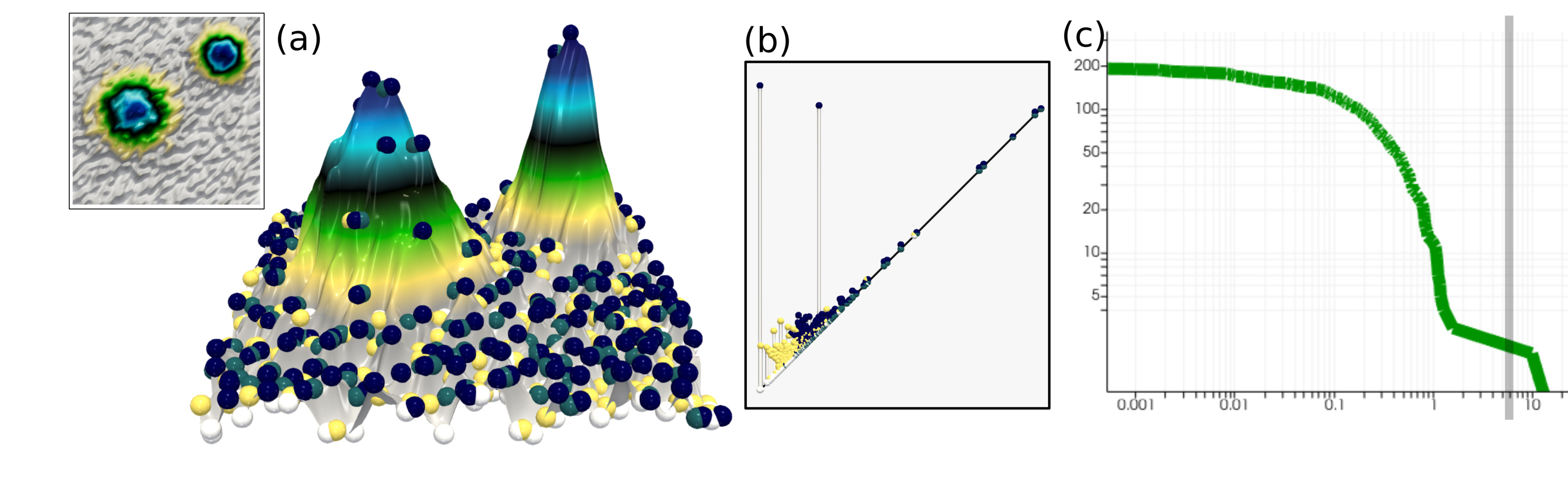
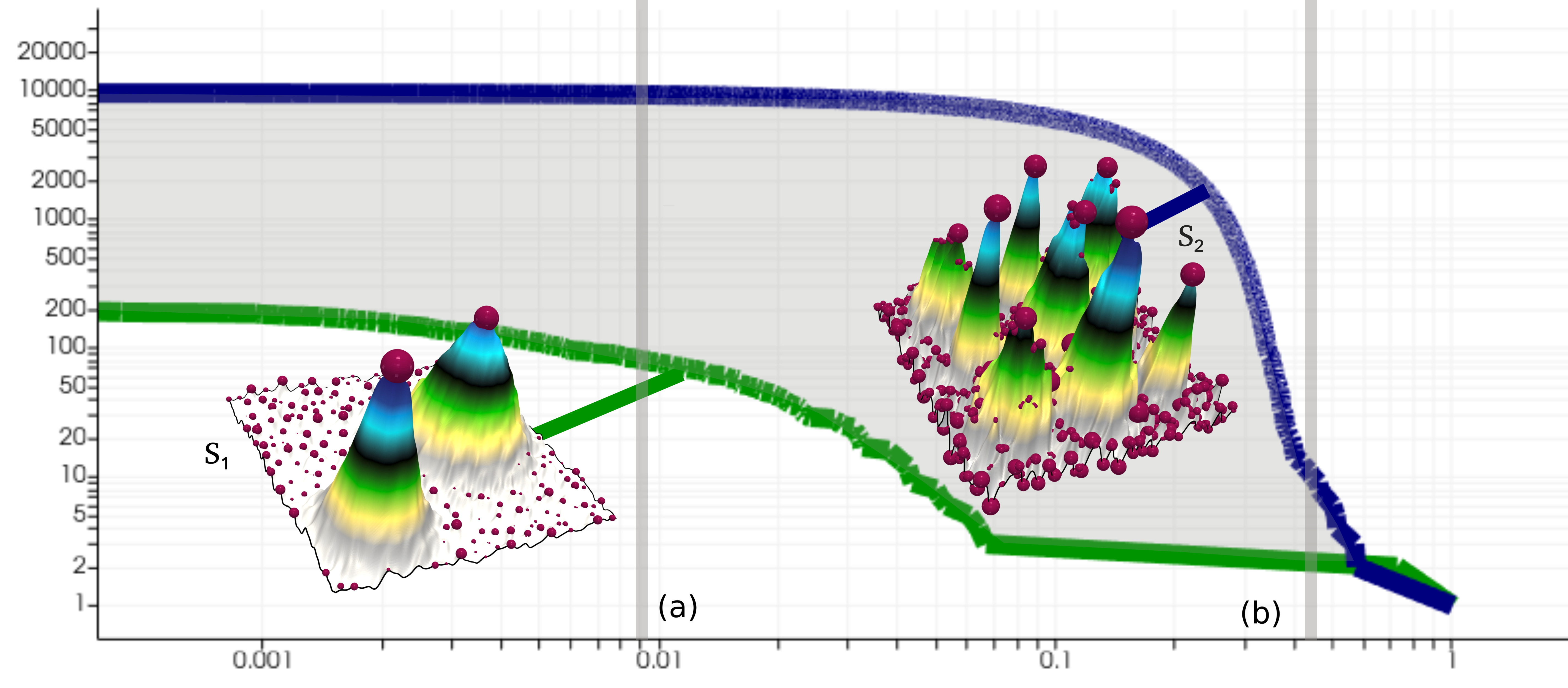
Topological Data Analysis protocols applied on an ensemble dataset of a Kelvin-Helmholtz instability. (a) The 180 members of the ensemble obtained with variations of timesteps, interpolation schemes, orders, resolutions and Riemann solvers (Tab. 1). (b) The top cluster represents the time separation of and for the flows and with the Wasserstein distance and the bottom cluster with the -norm. Red lines show the timestep separation with our clustering method whereas the sphere colors are the ground truth, illustrating the limitation of the -norm. (c) Persistence curve protocol: Differences between integrals of persistence curves (gray area) of the enstrophy computed with a SLAU2 solver, an order 7 TENO scheme and a resolution of for various configurations ( at , and at ). These integral differences exhibit the appearance of vortices (critical points) as the time increases. (d) Outlier distance protocol: Wasserstein distance matrix for 5 configurations , , , , computed with an order 7 WENO-Z interpolation scheme at . The sum of each row the configuration maximizing this distance between solvers and timesteps, here . (e) Unsupervised classification: Wasserstein distance matrix for the previous configurations with an order 7 WENO-Z interpolation scheme at . The clustering based on the Wasserstein distance and colored according to the Kmeans clustering method successfully segments the time steps.
Introduction
Flow turbulence is a phenomenon of major importance in fluid dynamics. It is characterized by chaotic changes in the motion of a flow (e.g. typical cigarette smoke patterns), which have a drastic impact in numerous applications (aeronautics, weather forecast, climate modeling, material sciences, astronomy, etc.). Although turbulence has been studied since the early stages of modern physics, its theoretical mastery remains incomplete [4] and the understanding of the Navier-Stokes equations, central in the description of fluid motion, is still considered as a major open challenge in mathematics and physics, as proven by the Clay Mathematics Institute selecting it to be among its celebrated Millennium Prize problems [34]. Thus, in engineering applications, the main practical solution available for the study of turbulence remains numerical simulation.
Problem introduction: However, many different numerical solvers can be used to simulate a given flow configuration, each solver being itself subject to several input parameters (such as domain resolution, interpolation scheme and order, etc.): when faced with such a wide variety, the main problem for users becomes the configuration itself of the simulation parameters. In particular, domain experts want not only to identify the solver configurations which produce the most realistic simulations, but they also want to discover configurations resulting in degraded but fast computations, which still produce simulations of acceptable realism. The fundamental problem behind such comparative analyses is that of comparing quantitatively turbulent flows. For instance, the quantitative realism of a simulation could be evaluated by comparing its outcome to a reference, either obtained by acquisition or by a highly detailed simulation considered as a ground-truth. However, the chaotic nature of turbulent flows makes their direct comparison with standard imaging tools impractical. For instance, turbulent flows which are considered similar at a high level by domain experts (in terms of the number and size of their vortices) are reported by classical metrics such as the norm as being very distant (Topological Analysis of Ensembles of Hydrodynamic Turbulent Flows An Experimental Study), as such pointwise measures are sensitive to mild geometrical variations in the data and miss global structural similarities in such a chaotic context. This observation motivates the consideration of alternative similarity estimation tools, which focus on the structure of the flow, rather than its raw geometry.
In that regard, Topological Data Analysis (TDA) [26] forms a family of generic, robust and efficient techniques, whose purpose is precisely to recover hidden implicit structural patterns in complex data, and to enable their reliable representation and comparison. As such, they provide potentially relevant alternatives to standard comparison measures used in scientific imaging, such as the norm. Moreover, the utility of TDA has been already demonstrated in a number of analysis and visualization tasks [51], with examples of successful applications in combustion [68, 16, 43], material sciences [45, 46, 33], bioimaging [21, 12, 2], quantum chemistry [39, 9, 82], or astrophysics [102, 101]. In particular, the critical points of flow vorticity indicators have been reported to appropriately capture the center of vortices [60, 18], as well as their importance, with the notion of topological persistence [30]. Such results provide additional evidence and consolidate the intuition that TDA could be a relevant framework for comparing turbulent flows.
The ambition of this application paper is to provide a comprehensive experimental evaluation of the above intuition, i.e. to assess the suitability of topological data representations and their associated analysis tools for the quantitative comparisons of turbulent flows. We shall focus on a specific type of turbulence that expresses itself in two dimensions (Kelvin-Helmholtz instability): it is a fair representative of generic turbulence (a.k.a. three-dimensional viscous turbulence) and allows for affordable high-resolution simulations to feed our study. Specifically, our study documents the usage of the persistence diagram of the maxima of flow enstrophy (an established indicator of vorticity for two-dimensional flows, Sec. 1) for the topological representation of 180 members of an ensemble of hydrodynamic turbulent flows, generated by a coarse sampling of the parameter space of five distinct solvers. We document five main hypotheses (Sec. 2) reported by domain experts, describing their expectations with regard to the variability among the flows generated by the distinct solver configurations. Then, we describe three evaluation protocols (Sec. 3) designed to assess the validation of the above hypotheses by standard comparison measures ( norm) on one hand, and by topological methods on the other. Specifically, these protocols exploit the persistence curve, the -Wasserstein distance between persistence diagrams [111] and -means in the -Wasserstein metric space [112]. Finally, we document the results of these protocols on the input ensemble (Sec. 4). We believe that the insights reported by our study bring a strong experimental evidence of the suitability of TDA for representing and comparing turbulent flows, thereby providing confidence in its usage by the fluid dynamics community in the future. Moreover, our flow data and evaluation protocols provide to the TDA community an application-approved benchmark for the evaluation and design of further topological distances in the future.
0.1 Related work
This section presents the literature related to our work. First, we discuss previous work dealing with (i) simulations of turbulent flow and their quantitative evaluation. Next, (ii) we review previous work dealing with topological methods for the analysis of ensemble data.
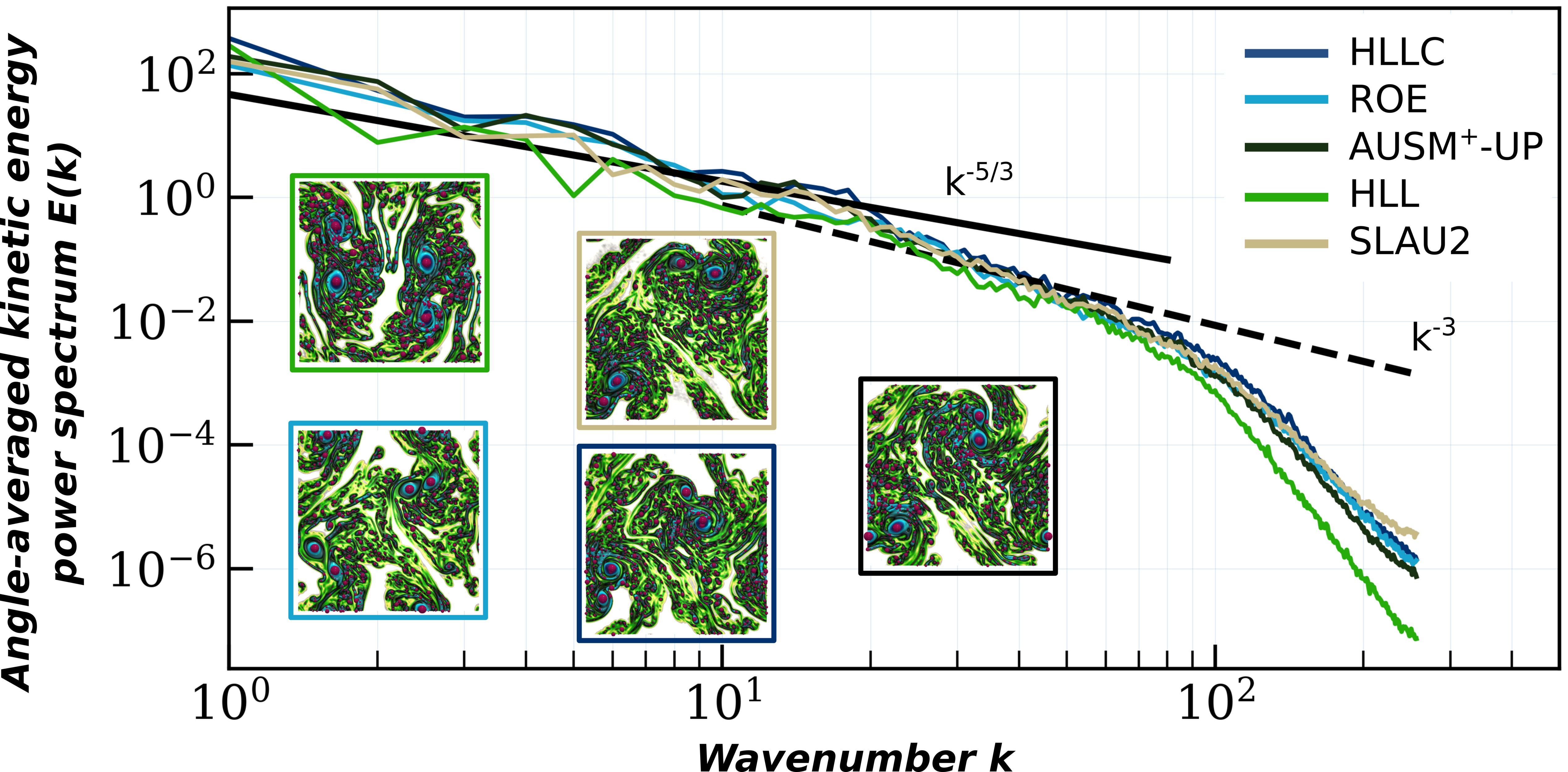
(i) Turbulent flow simulation. Turbulence is ubiquitous in nature, at all scales, from Higgs-Boson condensates [65] to a stirred cup of coffee to geophysical flows [66] to galaxy formation. While a significant literature in graphics [62, 116, 5] focused on the efficient generation of visually plausible turbulence, we focus in this work on the direct numerical simulation of the underlying physical equations, for engineering applications. A special distinction of 2D turbulence is that it is never realized in nature that, unless strongly constrained, always has some degree of three-dimensionality but rather it only exists in computer simulations. Two-dimensional turbulence has thus been studied extensively by the latter means e.g. for its importance as an idealization of meteorological flows [13], its role in the confinement of thermonuclear plasmas [66] but also as a cost-effective numerical testing ground for three-dimensional flows dynamical theories [104]. Most such studies focus either on validating predictions of theorists [65, 71] or on providing insights into the dynamic behavior of 2D eddies thanks to high-resolution simulations [71, 77]. The simulations are usually analyzed by considering macroscopic quantities such as the enstrophy (see below equation (3)), or by considering the Fourier decomposition of the 2D field (similar to Fig. 1)- integral indicators that make it near impossible to compare and/or classify the results of, say, a parametric study. Some efforts have been made recently [95] to provide the users with some guidelines to best choose the numerical methods and parameters for the simulation of 2D turbulence, but still using, mostly, the aforementioned integral, inaccurate, indicators. The present study aims at providing the workers in 2D turbulence with another tool to classify their results and best choose their settings, this time using mostly local indicators able to exploit the whole flow.
(ii) Topological methods for ensemble analysis. Concepts and algorithms from computational topology [26] have been investigated, adapted and extended by the visualization community for more than twenty years [51]. Specifically, a large body of literature has been dedicated to the analysis and visualization of flow data with topological methods and we refer the readers to a series of surveys on the topic [96, 38, 69, 89, 113, 19], including a recent iteration [47]. A substantial line of work [88, 84, 83] focused on extending topological techniques to uncertain vector fields, where flow variability is encoded via a pointwise estimator (e.g. an histogram) of an a priori vector distribution, but only few techniques explicitly focused on the analysis of flow variability in an ensemble. Specifically, several comparative visualization techniques have been proposed [97, 98, 55, 42, 57, 49, 117, 75]. Ferstl et al. [35] investigated the global structure of flow ensembles, by proposing a clustering approach of the members, based on a measure of streamline similarity. However, these techniques assume a mild geometrical variability within the ensemble and are therefore not suited to highly turbulent flows as studied in this work, where the geometry of the features (streamlines, vortices) chaotically changes from one ensemble member to the other (Topological Analysis of Ensembles of Hydrodynamic Turbulent Flows An Experimental Study), even upon only slight variations of the simulation input parameters. In certain application contexts, CFD experts often prefer to focus their analysis on (simpler to interpret) scalar descriptors generated from the flow, such as the kinetic energy (Fig. 1) or the enstrophy (Eq. 3). Such a transition to a scalar descriptor enables them to leverage the existing tools for scalar data analysis. For instance, several authors [60, 18] have shown that, given a relevant vorticity scalar descriptor, the center of the flow vortices could be reliably extracted and tracked over time, which supports the idea that topological methods for scalar data can be useful for the description of specific flow features. Thus, in the following, we describe the literature related to topological methods for scalar data. Popular topological representations include the persistence diagram [30, 26] which represents the population of features of interest in function of their salience, and which can be computed via matrix reduction [26, 7]. The Reeb graph [10], which describes the connectivity evolution of level sets, has also been widely studied and several efficient algorithms have been documented [86, 107, 85, 25], including parallel algorithms [41]. Efficient algorithms have also been documented for its variants, the merge and contour trees [105, 20] and parallel algorithms have also been described [76, 1, 22, 40]. The Morse-Smale complex [28, 27, 15], which depicts the global behavior of integral lines, is another popular topological data abstraction in visualization [24]. Robust and efficient algorithms have been introduced for its computation [93, 100, 44] based on Discrete Morse Theory [36]. Inspired by the literature in optimal transport [59, 79], the Wasserstein distance between persistence diagrams [26] (and its variant the Bottleneck distance [30]) have been extensively studied. In practice, it enables users to compare ensemble members based on their persistence diagrams. In our experimental study, we focus on this first, established topological tool for comparing the topology of ensemble members and we refer the reader to a recent survey [114] for a description of alternative metrics between topological descriptors. Several techniques have been proposed for summarizing the topological features in an ensemble or analyzing their variability. Favelier et al. [32] and Athawale et al. [3] introduced approaches for analyzing the variability of critical points and gradient separatrices respectively. Recent approaches aimed at summarizing an ensemble of topological descriptors by computing a notion of average descriptor, given a specific metric. This notion has been well studied for persistence diagrams [111, 67, 112], with direct applications to ensemble clustering [112], and analogies have been developed for merge trees [115, 90].
0.2 Contributions
This application paper makes the following new contributions:
-
1.
An evaluation procedure for distances between turbulent flows: We document 5 main hypotheses reported by domain experts, describing their expectations about flow variability within the studied ensemble (180 members). We contribute 3 evaluation protocols, to assess the validation of the hypotheses by a specific metric, given as a distance matrix between the members;
-
2.
A comprehensive experimental study: We provide a detailed experimental study of the ensemble under consideration for two distance metrics: (i) a standard distance used in scientific imaging (the norm) and (ii) an established topological distance between persistence diagrams (the -Wasserstein metric). Our experiments demonstrate the superiority of the topological distance to report as close solver configurations which are expected to be similar by domain experts. The insights reported by our study bring an experimental evidence of the suitability of the persistence diagram for representing and comparing turbulent flows, thereby providing to the fluid dynamics community confidence for its usage in future work;
-
3.
An application-approved benchmark: We provide as supplemental material (i) the input ensemble of 180 turbulent flows (see [81] for a direct link) and (ii) a python template script for reproducing our results. Our script supports the usage of custom distance matrices, thereby providing to the TDA community an application-approved template for the evaluation and design of further topological distances.
1 Background
This section presents the background used in this study in numerical simulation by presenting the equations, the interpolation schemes and the solvers implemented in our simulation code. Then the background in topological data analysis introduces the main notions used such as critical points, persistence diagrams or the Wasserstein distant metric.
1.1 Numerical simulation
In this work, we consider the two-dimensional compressible unsteady Euler equations for inviscid flows [78]:
| (1) |
where the subscripts indicate differentiation, is the vector of conservative dimensionless variables and and represent the inviscid fluxes in and direction respectively. Those vectors are defined as:
| (2) |
In the above expressions, denotes the time and and are the Cartesian coordinates. denotes density, and denote the and coordinates of the velocity vector , denotes the specific total energy and denotes the static pressure. The aforementioned mathematical model is described as it is implemented in the in-house code HYPERION (HYPERsonic vehicle design with Immersed bOuNdaries) whose primary capabilities as a massively parallel structured solver using immersed boundary conditions have already been discussed by Bridel-Bertomeu [17]. The present study uses only regular Cartesian grids with constant grid spacings (grid of pixels) in both directions of space, and , and will not rely on any immersed boundary condition during the computations presented later. This being said, the finite-volume method [70, 110, 108] is then employed for space discretization of the compressible Euler equations (1).
The 2D turbulence investigated in our work is generated using a Kelvin-Helmholtz instability (see [95] for a complete description) simulated with high-order low-dissipation reconstruction schemes of - and -order (Tab. 1). The numerical fluxes between the cells are obtained using a variety of Riemann solvers detail at the end of this section. To emulate turbulence in a infinite medium, all boundary conditions are set as periodic. One common measure of turbulence in two dimensions that we will rely on is the local enstrophy , defined locally as the square of the flow vorticity:
| (3) |
When solving numerically the Euler equations (Eq. 1), we start by interpolating the values of the flows at the cell interfaces. Then, we have to use an approximate Riemann solver [108] to solve the eponymous problem on those interfaces. In the remainder, we will expose the different methods used to make these two calculations.
Interpolation schemes. One problem in numerically solving the schemes is to be able to capture the strong discontinuities while capturing the small scales of the turbulence. In addition, we want to be as accurate as possible in our interpolation. To do this, researchers and engineers have developed several high-order reconstruction methods. A common scheme for solving compressible flows in the presence of strong discontinuities is the Weighted Essentially Non-Oscillatory (WENO) scheme [74]. Several variants of this scheme have been introduced, to improve its performances[58][54][52]. We are particularly interested in two families: the well-known robust but dissipative WENO-Z [14] and the TENO (T for Targeted) [37], which better discriminates scales [53].
Solvers. We have to solve the Riemann problems at the interfaces between the cells of the mesh. One solution is to use an exact Godunov solver [108] which takes into account a large number of nonlinear operations - too expensive however when calculating complex flows. Rather, researchers and engineers are interested in approximate Riemann solvers. The most used approximate solvers can be grouped in three large families: Flux Difference Splitting (FDS), Flux Vector Splitting (FVS) and Flux Type Splitting (FTS) [108]. In this section we will focus on two types of solvers in particular, Flux Difference Splitting solvers that work as a finite volume method to solve the Riemann problem and Flux Splitting Riemann solvers that combine the qualities of the other two families by separating kinematic and acoustic scales.
HLL (Harten, Lax, and van Leer) : FDS scheme developed by Harten et al. [50]. It does not take into account contact discontinuities, i.e. lines crossing two states. For turbulent phenomena, the interface between vortices will therefore be less described.
Roe and HLLC (Harten, Lax, and van Leer with Contact) : FDS type schemes developed by [109][94]. These two schemes are robust and thus allow to reproduce the strong discontinuity (shock) and takes into account the discontinuities of contact. Thus, with these schemes, the reconstruction of the vortices represented in our flows, is perform with more accuracy than with the HLL solver.
In its study on low speed Riemann solvers, [91] notice that the solvers are unable to obtain physical solutions. Therefore, there is a need for approximate Riemann solvers to accurately reconstruct both low and high speed flows. This is why we are interested in two flux type splitting (FTS) solvers, which take into account all velocities to obtain low Mach and high Mach physics solutions.
AUSM+-UP (Advection Upstream Splitting Method +UP) : By adding improvements [73] to the AUSM+ [72] solver Liou increases its level of accuracy for all speeds. This new solver takes into account contact discontinuities, reconstructs also strong discontinuities and gives physical solutions for all speeds.
SLAU2 (Simple Low-Dissipation AUSM 2) : the analysis of the dissipation pressure term of the AUSM+ [99] shows that it is too high for low speeds. The author decided to control the pressure flux and implemented the SLAU solver. This has been extended [63] so that the dissipation becomes proportional to the Mach number. This solver takes into account contact discontinuities, reconstructs also strong discontinuities and gives physical solutions for all speeds.
1.2 Topological data analysis
This section presents the topological background of our work. It contains definitions adapted from the Topology ToolKit [106]. We refer the reader to textbooks [26] for an introduction to topology.
Input data. The input data is given as an ensemble of piecewise linear (PL) scalar fields , with , defined on a PL 2-manifold . Specifically, represents the pointwise flow enstrophy (Sec. 1.1) and is the Freudenthal triangulation [48, 56] of a -dimensional regular grid, which is periodic in both dimensions ( is homeomorphic to a -dimensional torus). The triangulation is performed implicitly, by emulating the simplicial structure upon traversal queries. Thus it induces no memory overhead [106]. The scalar values are given at the vertices of and are linearly interpolated on the simplices of higher dimensions. is assumed to be injective on the vertices of . This is enforced in practice with a symbolic perturbation inspired by Simulation of Simplicity [31].
Critical points. Topological features in can be tracked with the notion of sub-level set, noted . It is defined as the pre-image of by . In particular, the topology of these sub-level sets (in 2D, their connected components and cycles) can only change at special locations. As continuously increases, the topology of changes at specific vertices of , called the critical points of [6], defined next. The star of a vertex , noted , is the set of its co-faces: . It can be interpreted as the smallest combinatorial neighborhood around . The link of , noted , is the set of the faces of the simplices of with empty intersection with : . The link of a vertex can be interpreted as the boundary of its star. The lower link of , noted , is given by the set of simplices of which only contain vertices lower than : . The upper link is defined symmetrically: . A vertex is regular if and only if both and are simply connected. For such vertices, the sub-level sets do not change their topology as they span . Otherwise, is a critical point. These can be classified with regard to their index . It is equal to for local minima (), to 2 for local maxima () and otherwise to 1 for saddles (Fig. 2a). In practice, is enforced to contain only isolated, non-degenerate critical points [31, 29]. In the case of the pointwise flow enstrophy, local maxima denote the center of vortices in the turbulent flow. However, since the critical point characterization is based on a classification which is only local (restricted to the link of each vertex), the slightest oscillation in the data results in practice in the appearance of spurious critical points, especially in the case of noisy data such as turbulent flows. This motivates the introduction of an importance measure on critical points, discussed next, in order to disambiguate vortices from noise.
Persistence diagrams. Several important measures for critical points have been studied [21], including topological persistence [30], which is tightly coupled to the notion of Persistence diagram [26], which we briefly describe here. Persistence assesses the importance of a critical point, based on the lifetime of the topological feature it created (or destroyed) in , as one continuously increase the isovalue . In particular, as increases, new connected components of are created at the minima of . The Elder rule [26] indicates that if two connected components, created at the minima and with , meet at a given saddle , the youngest of the two components (the one created at ) dies in favor of the oldest one (created at ). In this case, a persistence pair is created and its topological persistence is given by . All the local minima can be unambiguously paired following this strategy, while the global minimum is usually paired, by convention, with the global maximum. The symmetric reasoning can be applied to characterize, with saddle/maximum pairs, the life time of the independent cycles of . Persistence pairs are usually visualized with the Persistence diagram [26], which embeds each pair , with , as a point in the 2D plane, at location . The value is called the birth of the feature, while is called its death. The pair persistence can be visualized as the height of the point to the diagonal. Features with a high persistence stand out, away from the diagonal, while noisy features are typically located in its vicinity (Fig. 2b). The conciseness, stability [30] and expressiveness of this diagram made it a popular tool for data summarization tasks, as it provides visual hints about the number, ranges and salience of the features of interest. To compare two datasets and , persistence diagrams can be efficiently compared with the notion of -Wasserstein distance [23, 111, 61] (we leave the practical study of distances between more advanced topological descriptors [103, 90] to future work). This distance is based on a bipartite assignment optimization problem (between the points of the two diagrams to compare), for which exact [80] and approximate [8] implementations are publicly available [106, 11]. Specifically, we use in our approach the fast approximation scheme by Vidal et al. [112]. We refer the reader to [61, 112, 11] for further details. Once the -Wasserstein distance between two diagrams and is available (noted ), more advanced geometrical objects can be considered, such as Wasserstein barycenters [111, 112], which are diagrams minimizing the sum of their distance to an ensemble of diagrams, and which consequently, can be considered as a reliable representative of the ensemble. This notion of barycenter is conducive to the design of clustering algorithms. The -means algorithm can be easily extended, by using to measure distances between diagrams, and by considering as cluster centroid, at each iteration of the -means, the barycenter of the cluster.
Persistence curves. A popular, alternate, representation of persistence features is the notion of Persistence Curve, noted , which plots the population of persistent pairs as a function of their persistence. Specifically, it encodes the number of pairs (Y axis) whose persistence is larger than a threshold (X axis). For , is equal to the total number of persistence pairs, while for the largest values of , indicates the number of prominent, high-persistence features (Fig. 2c). In practice, large plateaus in this curve will indicate stable persistence ranges, for which no (or few) topological features are present in the data. These correspond to separations (vertical line, Fig. 2c) between populations of topological features of distinct persistence scales, typically the noise (low values) and the persistent features (high values).
2 Case Study
In this section, we give (i) a description of the ensemble (made publicly available [81]) representing the Kelvin Helmholtz Instabilities (KHI) computed on our institution’s facilities. Next, we state (ii) the challenges in understanding such phenomena and we provide (iii) theoretical hypothesis that our experimental protocols have to verify.
2.1 Data description
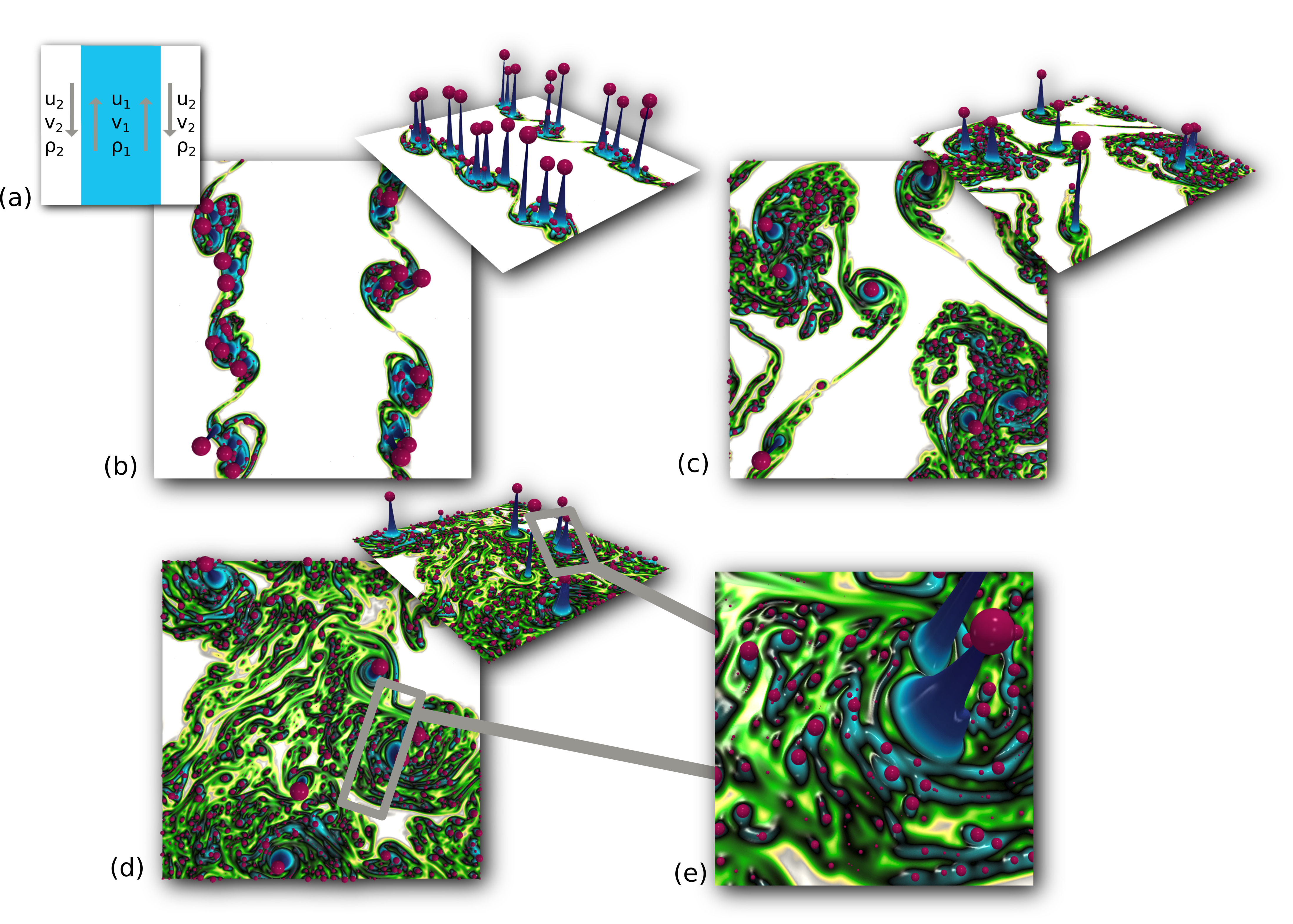
The initialization of the KHI was generated with two fluids of different densities (, ) (Fig. 3a). The different velocities of opposite direction () of the fluids create a shearing zone where the turbulence appears with the KHI (Fig. 3b). While the instability develops over time the main vortices grow (Fig. 3c). After a longer simulation time, the main structures keep evolving (Fig. 3d) and a large number of small-scale vortices appear in the vicinity of large-scale vortices (Fig. 3e) leading to a complex turbulent flow. This variation in vortex scale, in addition to the chaotic flow geometry, is notoriously challenging for the analysis of turbulent flows.
| Parameter | Resolution | Order | Time | Solver | Scheme | Total |
|---|---|---|---|---|---|---|
| HLL | ||||||
| 256 | 5 | t0 | SLAU2 | TENO | ||
| Value | 512 | 7 | t1 | AUSM+-UP | WENO-Z | |
| 1024 | t2 | Roe | ||||
| HLLC | ||||||
| Number | 3 | 2 | 3 | 5 | 2 | 180 |
The HYPERION simulation code introduced in Sec. 1.1 has been used to generate the ensemble dataset. All the simulations have been run on a supercomputer at our institution. Each simulation have been executed in parallel using 16 MPI processes and have been distributed over the supercomputer. The total simulation took about 745 CPU hours. The raw data has been dump on disk with the metadata stored in XDMF files and the scalar fields in HDF5 files leading to 14 GB for the entire ensemble dataset. We processed these results to extract the enstrophy scalar field (Eq. 3) and stored it to a VTK file format [64] using an image data structure for regular grids (VTI). This reduces the entire ensemble to 600 MB.
The ensemble dataset corresponds to different computational configurations for the same turbulent instability. HYPERION handles different parameter types such as scalars or enumerations, which allows the users to compute various numerical simulations in the same parametric study. The resolution of the 2D regular grid, the simulation time, the interpolation scheme, the order of interpolation and the Riemann solvers presented in Sec. 1 are our different parameters. Tab. 1 details the parameter types and values as well as the number of samples per parameter, leading overall to an ensemble of members illustrated Topological Analysis of Ensembles of Hydrodynamic Turbulent Flows An Experimental Studya. Each parameter value of Tab. 1 used to run the simulation has been stored as meta-data in the VTI files (i.e. Field Data in the VTK terminology) to keep track of the computational configuration for later analysis down the pipeline. In order to ease the exploration of the ensemble dataset, we defined a SQL-type database using the cinema database feature of TTK [106, 11]. This representation facilitates the extraction of sub-samples of the ensemble, based on standard SQL queries on the simulation parameters (Tab. 1).
2.2 Problem statement
Vehicle design, be it in an automotive or aeronautical context, is well known for its high number of constraints that are nowadays most often handled with the help of computational techniques. In the aeronautical world for instance, engineers today face an incredible challenge wherein they have to be able to predict, at the same time, integral quantities at the wall of the vehicle such as heat flux or pressure as well as three-dimensional phenomena such as flow discontinuities and turbulence. In other words, engineers have to deal with multiple types of physics and phenomena that have markedly different length- and time-scales but whose interactions are still of great importance to the accuracy of their predictions. With limited time and resources to conduct the computer-aided simulations, the traditional approach is to rely on numerical strategies that temporally average most of the three-dimensional phenomena and rely more or less on models of turbulence to yield a fast and reasonable forecast.
Even in such a context of approximate simulations, the choice of the ingredients of the numerical recipe matters - methods of reconstruction, Riemann solvers, etc. Making the right choices can indeed bring a significant increase in fidelity to the engineer, especially in terms of turbulence, by lessening the need for modeling and henceforth bring more margin in the design of the vehicle. Turbulence is however by nature a chaotic phenomenon and conducting a systematical study of the impact of the different numerical ingredients thereupon might prove tricky for a simple reason: beyond a certain level of accuracy, everything will look the same. Detecting the benefits of one method compared to another in that situation will be next to impossible - that is, with traditional techniques. We propose here to use the ability of topological analysis to discern features that stay otherwise hidden in traditional fluid dynamics postprocessing to help with the choice of the right numerical ingredients.
2.3 CFD Hypotheses
This section introduces the hypotheses provided by CFD experts, documenting their expectations about ensemble flow variability.
Hypothesis H1.
TENO induces more turbulence (i.e. more critical points) than
WENO-Z, for all configurations.
Hypothesis H2.
Order 5 and 7 are equivalent for Kelvin Helmholtz instabilities.
Hypothesis H3.
The HLL solver should provide a significantly distinct description, for all configurations.
Hypothesis H4.
The HLLC and Roe solvers should provide equivalent outputs for all configurations.
Hypothesis H5.
The
SLAU2 and AUSM+-UP solvers should provide equivalent outputs for all configurations.
The above hypotheses are direct consequences of observations, or design choices. For instance, the TENO scheme has been reported to capture turbulence more accurately [87], which is expressed by Hypothesis H1. Similar kinetic energy curves (Fig. 1) have been reported for the orders 5 and 7, which is expressed by Hypothesis H2. The HLL solver, which is a dissipative approach, is known to model contact discontinuities poorly in contrast to more recent solvers, which is expressed in Hypothesis H3 [108]. Finally, unlike the SLAU2 and AUSMUP (FTS type) solvers, the HLLC and RoE (FDS type) solvers have been reported to provide unphysical results at both low and high velocities (resulting in local oscillations in pressure and density), which is expressed in Hypotheses H4 and H5.
From a practical point of view, the validation of these hypotheses has a major impact for the engineers when setting up their simulations. For instance, the validation of the Hypothesis H1 would justify the usage of a more computationally expensive scheme (TENO), while the validation of the Hypothesis H2 would enable the usage of less computationally expensive orders (5 instead of 7). Finally, the validation of the Hypotheses H3, H4, and H5 would help engineers properly select the most appropriate solvers, based on their flow characteristics. Then, overall, the validation of these hypotheses would provide reliable rules-of-thumb for the tuning of the solvers, to achieve the best balance between accuracy and speed.
2.4 Baseline analysis
Traditional approaches for turbulent data analysis (Fig. 1) are based on an average of quantities of interest, such as flow energy (Sec. 0.1). The norm is another established distance for comparing scalar fields. Both strategies bear similarities in their averaging artifacts: they cannot distinguish the contribution of small structures from the global flow, because these are masked by the weight of larger vortices. Moreover, the -norm is also very sensitive to mild geometric variations, whereas the chaotic nature of turbulent flows induces major geometric variations between ensemble members. This motivates the usage of topological methods to capture features in the KHI that will help us compare the members (Sec. 4). In the remainder, we will systematically compare our protocols based on topological distances (Sec. 3) to the norm, considered as the baseline approach, and detailed comparisons will be provided (Sec. 4).
3 Evaluation protocols
In this section, we present 3 protocols which can be used to verify the hypotheses detailed in Sec. 2.3. One can directly use these algorithms on the ensemble dataset. It corresponds to the separation of the schemes and the independence of the orders, the unique behavior of the HLL solver and similarities in class of solvers.
3.1 Persistence curves
With this protocol (illustrated on toy examples, Fig. 4), we want to validate hypothesis H1 (Sec. 2.3) to discriminate the interpolation schemes TENO and WENO-Z regarding the differences in the enstrophy field. With this protocol, we also want to validate hypothesis H2 (Sec. 2.3) to confirm the independence of the orders [95]. To better characterize the vortices influencing the turbulence, we use persistence curves (Sec. 1.2). These curves will allow us to threshold the structures (the eddies) at different scales and thus to easily compare the number of small (Fig. 4a) and large (Fig. 4b) eddies using the integral of the persistence curve.
For the differentiation of the schemes, we take 5 simulation configurations where the physical time (), the resolution (, , ) and the order (5,7) are fixed per sample (Tab. 1). The variation is the interpolation scheme (TENO, WENO-Z). For the order independence, 5 configurations are also chosen by fixing the physical time (), the resolution (, , ), the scheme (TENO or WENO-Z). The variation is done on the order (5,7). Besides different input variations, this protocol is the same for testing H1 and H2.
The persistence curves are generated for all the samples. Then, we average the 5 persistence curves (one per solver) to obtain 2 average persistence curves with respect to the variable parameters (schemes or orders). Finally, we compute the difference of the integrals between the two averaged curves (grey area on Fig. 4). The small values on the curves under a persistence of correspond to numerical noise coming from the different simulation steps. They are removed from the computation of the integral with a threshold at (Fig. 4.a). The integral curve difference corresponds to our metric allowing to precisely describe the similarity in the topology of the critical points. Bigger is the integral, the more different the topology of the flow is. Thus, to verify hypothesis H1 related to the scheme, we want the difference of the integrals to be high. To verify hypothesis H2 related to the orders, we want the difference of the integrals to be close to zero.
3.2 Outlier distance profile
With this protocol (illustrated on toy examples, Fig. 5), we want to validate hypothesis H3 (Sec. 2.3), which means that for all the simulation configurations the HLL solver will be very different from other solvers to describe the Kelvin-Helmholtz instabilities. For this protocol, we take 5 simulation configurations where we fix the reconstruction (TENO or WENO-Z), the physical time (, , ), the mesh (), the order (5 or 7) and we vary the solvers. The 5 different computations describing the same turbulent flow obtained with the solvers (HLL, SLAU2, AUSM+-UP, HLLC and Roe) are analyzed regarding to the enstrophy.
A distance is used to compare the topology of the enstrophy. Many methods can be used to compute such a distance but in this protocol we focus on 2 metrics: the -norm distance directly on the values of the enstrophy and the Wasserstein distance on the persistence diagrams. One can inject other distances if needed. For the Wasserstein, the saddle-maximum persistence diagram is computed on each result. Then, they are grouped in a unique dataset to compute a persistence diagram distance matrix (Fig. 5). For the -norm, a distance matrix is also created where a line corresponds to the distance in the enstrophy field from one solver to the others.
Thus, the sum of the distances from one solver to the others is computed by summing the distances on one line of the matrix. The total distance of one solver to the others, for all configurations, is simply the sum of all these sum distances for every line of the matrix which correspond to the same solver. We finally obtain one global distance per solver for all configurations. Finally the difference between the distance of the HLL and the distance of the maximizer (the second value if HLL is the maximum) gives a separation score. If the difference is positive, then hypothesis H3 is verified whereas it is not if negative, because it means that another solver generates a flow topologically more different than the HLL. With this protocol, best separations are obtained for high absolute values.
3.3 Unsupervised classification
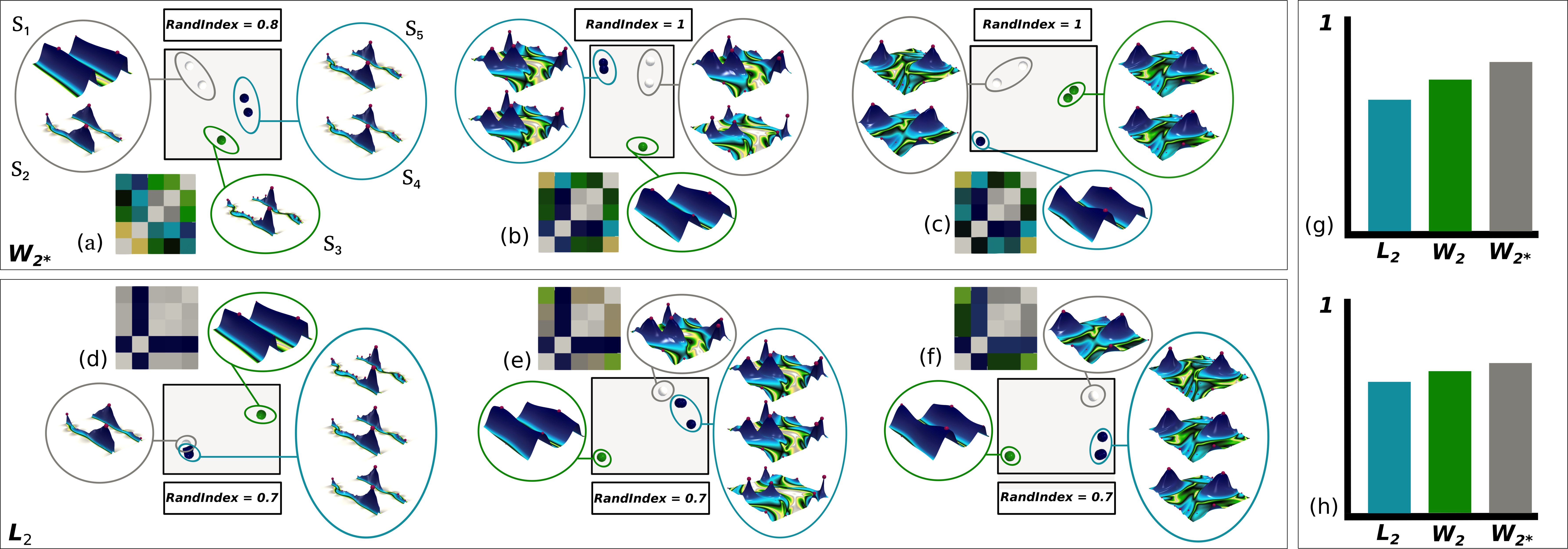
With the last protocol (illustrated on toy examples in Fig. 6), we want to validate hypotheses H4 and H5 (Sec. 2.3). We want to verify that the simulations with the Roe and HLLC solvers are topologically close (hypothesis H4) and the simulations with the AUSM+-UP and SLAU2 solvers are topologically close (hypothesis H5). To do so, three clustering methods will be used based on Wasserstein distances and the L2- norm(Sec. 1.2).
For the first two clustering methods, we start by computing distance matrix with the protocol of the outlier distance profile Sec. 3.2 using successively the Wasserstein distance and -norm matrices (Fig. 6a). We apply a dimension reduction to project the distances of the matrix according to 2 components (Sec. 1.2). This projection is used to generate clusters of the matrices with a k-means algorithm (Sec. 1.2) as illustrated on Fig. 6b. The third clustering method uses directly the persistence diagrams(Sec. 1.2) without using the distance matrix. All the persistence diagrams are merge into a single dataset to compute the Wasserstein distances between each diagram. The barycenter of persistence diagram is then used to directly compute a cluster, without dimension reduction, in the Wasserstein metric space [112] with the distance. Then a k-means algorithm (Sec. 1.2) is applied.
With these three classification methods, we obtain different associations of our configurations. Each association is going to be scored with a measure of similarities between the clusters regarding to a reference cluster using the Rand Index [92]. This Rand index has a value between 0 and 1, with 0 indicating that two clusters do not agree on any pair of points and 1 indicating that the data clusters are exactly the same. Based on the properties of the solvers used in the simulation code HYPERION and detailed in Sec. 1.1, we define our reference cluster such that the first partition contains the AUSM+-UP and SLAU2 solvers, the second partition the HLLC and Roe solvers and the third partition the HLL solver. The Rand Index is computed for each configuration and averaged per clustering method. This enables the ranking of the different solver behaviors. If the average Rand Index score is close to 1 then both hypotheses H4, showing similarity between the AUSM+-UP and SLAU2 solvers and H5, showing the isolation of the HLL solver, are verified.
4 Results
This section presents our experimental results and their interpretations, for the protocols presented in Sec. 3, applied on the ensemble data described in Sec. 2 (publicly available [81]).
4.1 Persistence curve study
We applied protocol 1 using the persistence curves, on our ensemble dataset of Kelvin-Helmotlz instability (KHI) to verify the hypotheses of separation of the schemes (H1) and the independence of the orders (H2)(Sec. 2.3). The input parameters are setup as detailed in Sec. 3, generating 36 studies. The terrains and curves on Fig. 7 illustrate the result for one configuration with a 5th order WENO-Z (Fig. 7.a), a 7th order WENO-Z (Fig. 7.c), a 5th order WENO-Z (Fig. 7.f) and a 5th order TENO (Fig. 7.h). For the scheme comparison, most of the averaged persistence curves for the TENO schemes (blue curves on Fig. 7g) are above the WENO-Z curves (green curves on Fig. 7g). The integral difference, between the average curves, obtain results between (Fig. 7.e), which demonstrates differences on the topology of the enstrophy between the interpolation methods as expected. Hypothesis H1 is verified on the KHI ensemble dataset. For the study on the independence of orders, we see that the averaged persistence curves are often close (Fig. 7b). However the integral differences obtained for this study show larger values for the WENO-Z, i.e in between (Fig. 7.d). This analysis highlights that orders play a more important role, in terms of topology of the vortices, for WENO-Z than for TENO. Moreover, we observe that this difference tends to increase at for both studies confirming that the flow is composed of a larger number of vortex as the simulation evolves. Hypothesis H2 is verified for the TENO solvers but not for the WENO-Z (Sec. 4.4).
4.2 Outlier distance profile study
To verify the HLL isolation states in hypothesis H3 (Sec. 2.3) on our ensemble dataset, we implemented our protocol 2 (Sec. 3) based on the Wasserstein distance and the -norm (Sec. 1.2). For this study we apply protocol 2 where the time and the resolution are fixed. The parameters that vary are the schemes (), the orders () and the solvers () (Tab. 1) thus generating 20 cases. All the distances have been computed according to the protocol of the outlier distance profile. These distances are represented by a global distance matrix where a line represents the 20 configurations (Wasserstein Fig. 8.a and norm Fig. 8.h) compared to a the HLL solver choosen as the reference. The matrix view of Fig. 8b and Fig. 8g show the KHI terrains and the distances of all configurations to the HLL solver.
The study has been done for all time steps and all resolutions generating nine distance matrices, for each distance. The histograms (Figs. 8.c and 8.e) show the average of these nine distance matrices for the Wasserstein distance and the -norm, expressed in terms of percentage according to the distance of HLL to the other solvers (HLL being the reference at 100%). In this case the percentage difference in distances to HLL are about 18% (Fig. 8.d) for the Wasserstein and 13% for the (Fig. 8.f). These large percentages confirm that HLL is a solver that behaves differently from others. As it does not take into account contact discontinuities, the interfaces between the vortices are much less defined than with the other solvers, resulting in a different number of vortices. From a physical point of view, this result confirms the isolation of HLL in all cases. From a topological point of view, it shows that the Wasserstein distance is the best at differentiating the HLL solver from the others (the distance gap is always bigger than the ). For this large study of 18 distance matrices , the hypothesis H3 is verified.
4.3 Unsupervised classification study
To improve our understanding on the behavior of the solvers into our simulation code, we implemented protocol 3 on the unsupervised classification (Sec. 3) to verified the hypotheses H4 and H5 (Sec. 2.3). The goal is to identify the separation of FDS type solvers from the FTS type solvers (Sec. 1.1). We are interested in the low Mach reconstructions (Sec. 1.1). The challenge comes from the fact that small vortices are reconstructed on only a few cells. So, we implemented protocol 3 with the distances and clustering method detailed in Sec. 3 leading to 5 simulation configurations (Tab. 1) with variable solvers. To focus on the small vortices we used a threshold of 0.38 persistence for the topological methods. On the KHI ensemble, we generated 36 clusters from the threshold persistence diagrams and obtain the Rand Index for all of them. Fig. 9.a, Fig. 9.b, Fig. 9.c show the clustering for the three timesteps and Fig. 9.d, Fig. 9.e, Fig. 9.f for the .
Histogram Fig. 9.h shows the average Rand Index for the three methods with a value of 0.63 for , 0.66 for and 0.71 for . There is very little difference between the topological and geometric results and each of the methods struggles to get the right cluster. Hypotheses H4 and H5 are not verified for high orders. However, to highlight the differences between solvers, it is necessary to use a reference reconstruction that barely captures small scale turbulence due to order dissipation (Sec. 1.1). Thus, we applied protocol 3 (Sec. 3) on a more restricted dataset at order 1. Histogram Fig. 9.g shows the average Rand Index at order 1 with the three methods leading to 0.63 for , 0.71 for and 0.78 for . In this case, we notice that for any reconstruction, the topological methods obtain better clustering. Moreover, the study with order 1 shows that the method enhances solver isolation. With this high score of the Rand Index hypotheses H4 and H5 are verified with the first order.
4.4 Unanticipated insights
During the analysis of the persistence curves generated by our protocol 1, we found significant differences on the topology of the enstrophy between the orders for the WENO-Z. By increasing the order, we increase the accuracy of our calculation that generates more structures into the turbulent flow. On the other hand, there is no difference between the orders obtained with the TENO. This means that other ingredients in the TENO reconstruction play an important role in the computation of the turbulence such as the separation of the scales. In addition, the persistence curves also allowed us to observe that the WENO-Z schemes produce more numerical errors than the TENO. As presented in Sec. 4.3, H4 and H5 hypotheses have not been verified for high orders. This means that the topological analysis does not capture the differences between the solvers. This may be due to the reconstructions which are accurate enough to calculate all velocities in the Kelvin-Helmholtz instability.
4.5 Limitations
As discussed in Sec. 4.2, in comparison to the norm, the Wasserstein distance improves the separation of the HLL solver, but only by (distance difference percentage). While this improvement may seem marginal, we would like to stress its significance given such challenging data, in particular with regard to the traditional approach based on kinetic energy, shown Fig. 1, where the five solvers can hardly be distinguished from each other. Similarly, we can see that the Rand Index score for the three clustering methods detailed in Sec. 4.3 are quite close to each other as illustrated on Fig. 9.h. These close scores are due to the interpolations schemes (Sec. 1.1) which cover up the differences between the different solvers. In other words, the variations in vortex distributions induced by the choice of solver are too subtle, given the importance of the interpolation order on the outcome. As shown in Fig. 9 (top), we were still able to overcome this limitation by considering a reconstruction that is not dedicated to turbulence, i.e. an upwind scheme of order 1. This enabled us to exaggerate the impact of the solvers, thereby allowing us to validate hypotheses H4 and H5 as reported in Sec. 4.3.
5 Conclusion
In this paper, we have presented an experimental protocol for the comparison of numerical methods on a Kelvin-Helmholtz instability using topological analysis. An ensemble dataset of 180 members has been computed for this instability by a simulation code developed in our institution and running on a supercomputer. While traditional approaches based on the kinetic energy (Fig. 1) only enable to validate the physical conformity of the generated flow, our overall approach provides finer analyses. In particular, the protocol using the persistence curves (Sec. 3.1) allowed us to observe differences between the TENO and WENO-Z reconstructions. It also confirms an independence of the reconstruction order (5 or 7) when using the TENO scheme allowing practical computational speedup, without loss of precision. The protocol based on the Wasserstein distance (Sec. 3.2) succeeded in discriminating the HLL solvers from other configurations, validating the use of such a topological analysis to confirm domain field expectations. The last protocol, based on recent clustering methods (Sec. 4.3) successfully differentiates the topology of computations based on FDS (Flux Difference Splitting) and FTS (Flux Type Splitting) solvers. Overall, the validation of the hypotheses reported by CFD experts (Sec. 2.3) provides reliable indications for the tuning of a flow simulation, to help CFD users achieve the best balance between computation accuracy and speed.
The results obtained in this experimental study also show the viability of topological methods for the representation and comparison of Kelvin-Helmholtz instabilities. The interesting aspect of these topological protocols is that the numerical method comparisons are based on physical differences rather than on unreliable, low-level, pointwise measures. The direction we wish to take now, for our future work, is the extension of these protocols to 3D datasets of external hypersonics aerodynamics. Another direction we want to investigate is the evaluation of other tools used in the protocol such as new topological distances [90] or clustering methods. Finally, this experimental study allows us, with confidence, to consider applying these protocols to other hydrodynamic turbulent flows studied in our institution in the domain of hypersonic vehicle design.
Acknowledgements.
This work is partially supported by the European Commission grant ERC-2019-COG “TORI” (ref. 863464, https://erc-tori.github.io/).References
- [1] A. Acharya and V. Natarajan. A parallel and memory efficient algorithm for constructing the contour tree. In IEEE PV, 2015.
- [2] K. Anderson, J. Anderson, S. Palande, and B. Wang. Topological data analysis of functional MRI connectivity in time and space domains. In MICCAI Workshop on Connectomics in NeuroImaging, 2018.
- [3] T. M. Athawale, D. Maljovec, C. R. Johnson, V. Pascucci, and B. Wang. Uncertainty visualization of 2d morse complex ensembles using statistical summary maps. CoRR, abs/1912.06341, 2019.
- [4] J. C. Baez. Open Questions in Physics. Technical report, UC Riverside, Department of Mathematics, 2006.
- [5] K. Bai, C. Wang, M. Desbrun, and X. Liu. Predicting high-resolution turbulence details in space and time. ACM Trans. Graph., 2021.
- [6] T. F. Banchoff. Critical points and curvature for embedded polyhedral surfaces. The American Mathematical Monthly, 1970.
- [7] U. Bauer, M. Kerber, and J. Reininghaus. Distributed computation of persistent homology. In Algo. Eng. and Exp., 2014.
- [8] D. P. Bertsekas. A new algorithm for the assignment problem. Mathematical Programming, 1981.
- [9] H. Bhatia, A. G. Gyulassy, V. Lordi, J. E. Pask, V. Pascucci, and P.-T. Bremer. Topoms: Comprehensive topological exploration for molecular and condensed-matter systems. J. of Comp. Chem., 2018.
- [10] S. Biasotti, D. Giorgio, M. Spagnuolo, and B. Falcidieno. Reeb graphs for shape analysis and applications. TCS, 2008.
- [11] T. Bin Masood, J. Budin, M. Falk, G. Favelier, C. Garth, C. Gueunet, P. Guillou, L. Hofmann, P. Hristov, A. Kamakshidasan, C. Kappe, P. Klacansky, P. Laurin, J. Levine, J. Lukasczyk, D. Sakurai, M. Soler, P. Steneteg, J. Tierny, W. Usher, J. Vidal, and M. Wozniak. An Overview of the Topology ToolKit. In TopoInVis, 2019.
- [12] A. Bock, H. Doraiswamy, A. Summers, and C. T. Silva. TopoAngler: Interactive Topology-Based Extraction of Fishes. IEEE TVCG, 2018.
- [13] G. Boffetta and R. E. Ecke. Two-dimensional turbulence. Annual Review of Fluid Mechanics, 2011.
- [14] R. Borges, M. Carmona, B. Costa, and W. S. Don. An improved weighted essentially non-oscillatory scheme for hyperbolic conservation laws. Journal of Computational Physics, 2008.
- [15] P. Bremer, H. Edelsbrunner, B. Hamann, and V. Pascucci. A Multi-Resolution Data Structure for 2-Dimensional Morse Functions. In Proc. of IEEE VIS, 2003.
- [16] P. Bremer, G. Weber, J. Tierny, V. Pascucci, M. Day, and J. Bell. Interactive exploration and analysis of large scale simulations using topology-based data segmentation. IEEE TVCG, 2011.
- [17] T. Bridel-Bertomeu. Immersed boundary conditions for hypersonic flows using eno-like least-square reconstruction. Comp. & Flu., 2021.
- [18] T. Bridel-Bertomeu, B. Fovet, J. Tierny, and F. Vivodtzev. Topological Analysis of High Velocity Turbulent Flow. In IEEE LDAV, 2019.
- [19] R. Bujack, L. Yan, I. Hotz, C. Garth, and B. Wang. State of the art in time-dependent flow topology: Interpreting physical meaningfulness through mathematical properties. CGF, 2020.
- [20] H. Carr, J. Snoeyink, and U. Axen. Computing contour trees in all dimensions. In Symp. on Dis. Alg., 2000.
- [21] H. A. Carr, J. Snoeyink, and M. van de Panne. Simplifying Flexible Isosurfaces Using Local Geometric Measures. In IEEE VIS, 2004.
- [22] H. A. Carr, G. H. Weber, C. M. Sewell, and J. P. Ahrens. Parallel peak pruning for scalable SMP contour tree computation. In LDAV, 2016.
- [23] D. Cohen-Steiner, H. Edelsbrunner, and J. Harer. Stability of persistence diagrams. In SoCG, 2005.
- [24] L. De Floriani, U. Fugacci, F. Iuricich, and P. Magillo. Morse complexes for shape segmentation and homological analysis: discrete models and algorithms. CGF, 2015.
- [25] H. Doraiswamy and V. Natarajan. Computing reeb graphs as a union of contour trees. IEEE TVCG, 2013.
- [26] H. Edelsbrunner and J. Harer. Computational Topology: An Introduction. American Mathematical Society, 2009.
- [27] H. Edelsbrunner, J. Harer, V. Natarajan, and V. Pascucci. Morse-smale complexes for piecewise linear 3-manifolds. In SoCG, 2003.
- [28] H. Edelsbrunner, J. Harer, and A. Zomorodian. Hierarchical morse complexes for piecewise linear 2-manifolds. In SoCG, 2001.
- [29] H. Edelsbrunner, J. Harer, and A. Zomorodian. Hierarchical Morse-Smale complexes for piecewise linear 2-manfiolds. DCG, 2003.
- [30] H. Edelsbrunner, D. Letscher, and A. Zomorodian. Topological persistence and simplification. DCG, 2002.
- [31] H. Edelsbrunner and E. P. Mucke. Simulation of simplicity: a technique to cope with degenerate cases in geometric algorithms. ACM ToG, 1990.
- [32] G. Favelier, N. Faraj, B. Summa, and J. Tierny. Persistence Atlas for Critical Point Variability in Ensembles. IEEE TVCG, 2018.
- [33] G. Favelier, C. Gueunet, and J. Tierny. Visualizing ensembles of viscous fingers. In IEEE SciVis Contest, 2016.
- [34] C. L. Fefferman. Existence and Smoothness of the Navier-Stokes Equation. Technical report, Clay Mathematics Institute, 2000. https://www.claymath.org/sites/default/files/navierstokes.pdf.
- [35] F. Ferstl, K. Bürger, and R. Westermann. Streamline variability plots for characterizing the uncertainty in vector field ensembles. IEEE TVCG, 2016.
- [36] R. Forman. A User’s Guide to Discrete Morse Theory. AM, 1998.
- [37] L. Fu, X. Y. Hu, and N. A. Adams. A family of high-order targeted eno schemes for compressible-fluid simulations. Journal of Computational Physics, 305:333–359, 2016.
- [38] C. Garth and X. Tricoche. Topology- and feature-based flow visualization: Methods and applications. In VLDUDS, 2006.
- [39] D. Guenther, R. Alvarez-Boto, J. Contreras-Garcia, J.-P. Piquemal, and J. Tierny. Characterizing molecular interactions in chemical systems. IEEE TVCG, 2014.
- [40] C. Gueunet, P. Fortin, J. Jomier, and J. Tierny. Task-Based Augmented Contour Trees with Fibonacci Heaps. IEEE TPDS, 2019.
- [41] C. Gueunet, P. Fortin, J. Jomier, and J. Tierny. Task-based Augmented Reeb Graphs with Dynamic ST-Trees. In EGPGV, 2019.
- [42] H. Guo, W. He, T. Peterka, H. Shen, S. M. Collis, and J. J. Helmus. Finite-time lyapunov exponents and lagrangian coherent structures in uncertain unsteady flows. IEEE Trans. Vis. Comput. Graph., 2016.
- [43] A. Gyulassy, P. Bremer, R. Grout, H. Kolla, J. Chen, and V. Pascucci. Stability of dissipation elements: A case study in combustion. CGF, 2014.
- [44] A. Gyulassy, P. Bremer, and V. Pascucci. Shared-Memory Parallel Computation of Morse-Smale Complexes with Improved Accuracy. IEEE TVCG, 2018.
- [45] A. Gyulassy, M. A. Duchaineau, V. Natarajan, V. Pascucci, E. Bringa, A. Higginbotham, and B. Hamann. Topologically clean distance fields. IEEE TVCG, 2007.
- [46] A. Gyulassy, A. Knoll, K. Lau, B. Wang, P. Bremer, M. Papka, L. A. Curtiss, and V. Pascucci. Interstitial and interlayer ion diffusion geometry extraction in graphitic nanosphere battery materials. IEEE TVCG, 2015.
- [47] T. Günther and I. Baeza Rojo. Introduction to Vector Field Topology. In TopoInVis. Springer, 2021.
- [48] H. Freudenthal. Simplizialzerlegungen von beschrankter Flachheit. Annals of Mathematics, 43:580–582, 1942.
- [49] K. Hanser, O. Klein, B. Rieck, B. Wiebe, T. Selz, M. Piatkowski, A. Sagristà, B. Zheng, M. Lukácová, G. Craig, H. Leitte, and F. Sadlo. Visualization of Parameter Sensitivity of 2D Time-Dependent Flow. In Proc. of International Symposium on Visual Computing, 2018.
- [50] A. Harten, P. D. Lax, and B. v. Leer. On upstream differencing and godunov-type schemes for hyperbolic conservation laws. SIAM review, 25(1):35–61, 1983.
- [51] C. Heine, H. Leitte, M. Hlawitschka, F. Iuricich, L. De Floriani, G. Scheuermann, H. Hagen, and C. Garth. A survey of topology-based methods in visualization. CGF, 2016.
- [52] A. K. Henrick, T. D. Aslam, and J. M. Powers. Mapped weighted essentially non-oscillatory schemes: achieving optimal order near critical points. Journal of Computational Physics, 2005.
- [53] X. Hu and N. A. Adams. Scale separation for implicit large eddy simulation. Journal of Computational Physics, 2011.
- [54] X. Hu, Q. Wang, and N. A. Adams. An adaptive central-upwind weighted essentially non-oscillatory scheme. J. of Comp. Phys., 2010.
- [55] M. Hummel, H. Obermaier, C. Garth, and K. I. Joy. Comparative visual analysis of lagrangian transport in CFD ensembles. IEEE TVCG, 2013.
- [56] H.W. Kuhn. Some combinatorial lemmas in topology. IBM Journal of Research and Development, 45:518–524, 1960.
- [57] M. Jarema, J. Kehrer, and R. Westermann. Comparative visual analysis of transport variability in flow ensembles. J. WSCG, 2016.
- [58] G.-S. Jiang and C.-W. Shu. Efficient implementation of weighted eno schemes. Journal of computational physics, 126(1):202–228, 1996.
- [59] L. Kantorovich. On the translocation of masses. AS URSS, 1942.
- [60] J. Kasten, J. Reininghaus, I. Hotz, and H. Hege. Two-dimensional time-dependent vortex regions based on the acceleration magnitude. IEEE TVCG, 2011.
- [61] M. Kerber, D. Morozov, and A. Nigmetov. Geometry helps to compare persistence diagrams. ACM J. of Exp. Algo., 2016.
- [62] T. Kim, N. Thürey, D. L. James, and M. H. Gross. Wavelet turbulence for fluid simulation. ACM Trans. Graph., 2008.
- [63] K. Kitamura and E. Shima. Towards shock-stable and accurate hypersonic heating computations: A new pressure flux for ausm-family schemes. Journal of Computational Physics, 245:62–83, 2013.
- [64] Kitware, Inc. The Visualization Toolkit User’s Guide, January 2003.
- [65] R. H. Kraichnan. Inertial ranges in two-dimensional turbulence. Physics of Fluids, 10:1417–1423, 1967. doi: 10 . 1063/1 . 1762301
- [66] R. H. Kraichnan and D. Montgomery. Two-dimensional turbulence. Rep. Prog. Phys, 43:547, 1980.
- [67] T. Lacombe, M. Cuturi, and S. Oudot. Large Scale computation of Means and Clusters for Persistence Diagrams using Optimal Transport. In NIPS, 2018.
- [68] D. E. Laney, P. Bremer, A. Mascarenhas, P. Miller, and V. Pascucci. Understanding the structure of the turbulent mixing layer in hydrodynamic instabilities. IEEE TVCG, 2006.
- [69] R. S. Laramee, H. Hauser, L. Zhao, and F. H. Post. Topology-based flow visualization, the state of the art. In TopoInVis. 2007.
- [70] R. J. LeVeque et al. Finite volume methods for hyperbolic problems, vol. 31. Cambridge university press, 2002.
- [71] D. K. Lilly. Two-dimensional turbulence generated by energy sources at two scales. Journal of Atmospheric Sciences, 1989.
- [72] M.-S. Liou. A sequel to ausm: Ausm+. J. Comp. Phys., 1996.
- [73] M.-S. Liou. A sequel to ausm, part ii: Ausm+-up for all speeds. J. Comp. Phys., 2006.
- [74] X.-g. Liu, S. Osher, and T. Chan. Weighted essentially non-oscillatory schemes. Journal of computational physics, 115(1):200–212, 1994.
- [75] A. P. Lohfink and C. Garth. Visitation graphs: Interactive ensemble visualization with visitation maps. In iPMVM, 2020.
- [76] S. Maadasamy, H. Doraiswamy, and V. Natarajan. A hybrid parallel algorithm for computing and tracking level set topology. In Proc. of HiPC, 2012.
- [77] M. Maltrud and G. Vallis. Energy spectra and coherent structures in forced two-dimensional and -planeturbulence. J. Flu. Mech., 1991.
- [78] K. Masatsuka. I do Like CFD, vol. 1, vol. 1. Lulu. com, 2013.
- [79] G. Monge. Mémoire sur la théorie des déblais et des remblais. Académie Royale des Sciences de Paris, 1781.
- [80] J. Munkres. Algorithms for the assignment and transportation problems. J. of the Society for Industrial and Applied Mathematics, 1957.
- [81] F. Nauleau, F. Vivodtzev, T. Bridel-Bertomeu, H. Beaugendre, and J. Tierny. Benchmark Ensemble Data. https://drive.google.com/drive/folders/1CAxn4SkkU-u5cQD2bdPn4NNxwQMP7oa7?usp=sharing, 2022.
- [82] M. Olejniczak, A. S. P. Gomes, and J. Tierny. A Topological Data Analysis Perspective on Non-Covalent Interactions in Relativistic Calculations. International Journal of Quantum Chemistry, 2019.
- [83] M. Otto, T. Germer, H.-C. Hege, and H. Theisel. Uncertain 2D vector field topology. CGF, 2010.
- [84] M. Otto, T. Germer, and H. Theisel. Uncertain topology of 3D vector fields. IEEE PV, 2011.
- [85] S. Parsa. A deterministic o(m log m) time algorithm for the reeb graph. In SoCG, 2012.
- [86] V. Pascucci, G. Scorzelli, P. T. Bremer, and A. Mascarenhas. Robust on-line computation of Reeb graphs: simplicity and speed. ACM ToG, 2007.
- [87] J. Peng, S. Liu, S. Li, K. Zhang, and Y. Shen. An efficient targeted eno scheme with local adaptive dissipation for compressible flow simulation. Journal of Computational Physics, 425:109902, 2021.
- [88] C. Petz, K. Pöthkow, and H.-C. Hege. Probabilistic local features in uncertain vector fields with spatial correlation. CGF, 2012.
- [89] A. Pobitzer, R. Peikert, R. Fuchs, B. Schindler, A. Kuhn, H. Theisel, K. Matkovic, and H. Hauser. The state of the art in topology-based visualization of unsteady flow. CGF, 2011.
- [90] M. Pont, J. Vidal, J. Delon, and J. Tierny. Wasserstein Distances, Geodesics and Barycenters of Merge Trees. IEEE TVCG, 2021.
- [91] F. Qu, C. Yan, J. Yu, and D. Sun. A study of parameter-free shock capturing upwind schemes on low speeds’ issues. C. T. S., 2014.
- [92] W. M. Rand. Objective criteria for the evaluation of clustering methods. Journal of the American Statistical association, 1971.
- [93] V. Robins, P. J. Wood, and A. P. Sheppard. Theory and Algorithms for Constructing Discrete Morse Complexes from Grayscale Digital Images. IEEE Trans. Pattern Anal. Mach. Intell., 2011.
- [94] P. L. Roe. Approximate riemann solvers, parameter vectors, and difference schemes. Journal of computational physics, 1981.
- [95] O. San and K. Kara. Evaluation of riemann flux solvers for weno reconstruction schemes: Kelvin–helmholtz instability. C. & F., 2015.
- [96] G. Scheuermann and X. Tricoche. Topological methods for flow visualization. In The Visualization Handbook, pp. 341–356. 2005.
- [97] M. Schlemmer, M. Heringer, F. Morr, I. Hotz, M. Hering-Bertram, C. Garth, W. Kollmann, B. Hamann, and H. Hagen. Moment Invariants for the Analysis of 2D Flow Fields. IEEE TVCG, 2007.
- [98] D. Schneider, J. Fuhrmann, W. Reich, and G. Scheuermann. A variance based FTLE-like method for unsteady uncertain vector fields. In TopoInVis, 2012.
- [99] E. Shima and K. Kitamura. On new simple low-dissipation scheme of ausm-family for all speeds. In AIAA Aerospace Sciences, 2009.
- [100] N. Shivashankar and V. Natarajan. Parallel Computation of 3D Morse-Smale Complexes. CGF, 2012.
- [101] N. Shivashankar, P. Pranav, V. Natarajan, R. van de Weygaert, E. P. Bos, and S. Rieder. Felix: A topology based framework for visual exploration of cosmic filaments. IEEE TVCG, 2016.
- [102] T. Sousbie. The persistent cosmic web and its filamentary structure: Theory and implementations. Royal Astronomical Society, 2011.
- [103] R. Sridharamurthy, T. B. Masood, A. Kamakshidasan, and V. Natarajan. Edit distance between merge trees. IEEE TVCG, 2020.
- [104] P. Tabeling. Two-dimensional turbulence: a physicist approach, 2002.
- [105] S. Tarasov and M. Vyali. Construction of contour trees in 3d in o(n log n) steps. In SoCG, 1998.
- [106] J. Tierny, G. Favelier, J. A. Levine, C. Gueunet, and M. Michaux. The Topology ToolKit. IEEE TVCG, 2017. https://topology-tool-kit.github.io/.
- [107] J. Tierny, A. Gyulassy, E. Simon, and V. Pascucci. Loop surgery for volumetric meshes: Reeb graphs reduced to contour trees. IEEE TVCG, 2009.
- [108] E. F. Toro. Riemann solvers and numerical methods for fluid dynamics: a practical introduction. Springer Science & Business Media, 2013.
- [109] E. F. Toro, M. Spruce, and W. Speares. Restoration of the contact surface in the hll-riemann solver. Shock waves, 4(1):25–34, 1994.
- [110] J. A. Trangenstein. Numerical Solution of Hyperbolic Partial Differential Equations. Cambridge University Press, 2007.
- [111] K. Turner, Y. Mileyko, S. Mukherjee, and J. Harer. Fréchet Means for Distributions of Persistence Diagrams. DCG, 2014.
- [112] J. Vidal, J. Budin, and J. Tierny. Progressive Wasserstein Barycenters of Persistence Diagrams. IEEE TVCG, 2019.
- [113] W. Wang, W. Wang, and S. Li. From numerics to combinatorics: a survey of topological methods for vector field visualization. Journal of Visualization, 2016.
- [114] L. Yan, T. B. Masood, R. Sridharamurthy, F. Rasheed, V. Natarajan, I. Hotz, and B. Wang. Scalar field comparison with topological descriptors: Properties and applications for scientific visualization. CGF, 2021.
- [115] L. Yan, Y. Wang, E. Munch, E. Gasparovic, and B. Wang. A structural average of labeled merge trees for uncertainty visualization. IEEE TVCG, 2019.
- [116] M. Zhang, S. Liu, H. Sun, W. Si, and Y. Qian. Hybrid vortex model for efficiently simulating turbulent smoke. In ACM VRCAI, 2014.
- [117] B. Zheng, B. Rieck, H. Leitte, and F. Sadlo. Visualization of Equivalence in 2D Bivariate Fields. CGF, 2019.