We examine the effect of side walls on the linear stability of falling liquid films by combining theoretical modeling and experimental techniques. This approach to the problem introduces the missing theoretical background for the spanwise confinement effect reported in the literature, which is limited to experiments only. Additionally, the theoretical stability model offers the opportunity to explore a wide range of flow parameters, which was not possible due to the experimental techniques restrictions. This monograph is organized as follows, In section 2, we discuss the non-dimensional governing equations alongside the dimensionless parameters. The base state and the linear stability analysis are also presented in the same section. The experimental set up and the linear stability measurement technique are presented in section LABEL:sec:exp_Setup. Our results consisting of validating the numerical stability model with the experiments followed by extensive theoretical investigation of different aspects of the problem are presented in section LABEL:sec:results. Finally, we present our concluding remarks and potential direction of investigations in section LABEL:sec:conclusion.

2 Theoretical formulation

The theoretical formulation of the problem is presented in this section. We start with listing the non-dimensional governing equations, and the associated walls and the free surface boundary conditions, in section 2.1. Afterwards, we present the base state solution (section 2.2) followed by the methodology to linear stability analysis (section 2.3). Finally, the numerical approach to solve the problem is presented in section LABEL:numerical_method.

2.1 Non-dimensional governing equations:

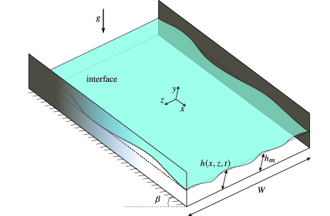
Figure 1: Schematic diagram of liquid film falling down an inclined channel. $h(x,z,t)$ is the local film thickness, and $h_{m}$ is the mean film thickness.

We consider a three-dimensional liquid film running down a tilted channel due to gravity $g$ (figure 1). The channel has a width $W$ and forms an angle $\beta$ with the horizontal. The density $\rho$ and dynamic viscosity $\mu$ are constant, while the kinematic viscosity $\nu$ is given by $\nu=\mu/\rho$. We use the Cartesian coordinates $(x,y,z)$, where $x$ corresponds to the streamwise direction, $y$ is bottom wall normal increasing into the liquid, and $z$ is in the spanwise direction. The left and right walls of the channel are located at $z=0$ and $z=W$, respectively. The following length, time, velocity and pressure scales are introduced in order to non-dimensionalize the system:

$\quad h\rightarrow h_{m}\ h^{*},\quad$	$\quad(x,y,z)\rightarrow h_{m}\ (x^{*},y^{*},z^{*}),\qquad$	$\quad W\rightarrow h_{m}\ W^{*},\quad$
$\quad t\rightarrow h_{m}^{2}/\nu\ t^{*},\quad$	$\quad(u,v,w)\rightarrow\nu/h_{m}\ (u^{*},v^{*},w^{*}),\quad$	$\quad p\rightarrow\rho\nu^{2}/h_{m}^{2}\ p^{*},\quad$

where $h_{m}$ is the mean film thickness. By using these scales and dropping the stars for simplicity, we obtain the dimensionless governing equations, continuity and Navier-Stokes, as follows:

& ∂_x u + ∂_y v + ∂_z w = 0,
∂_t u +u ⋅∇u = - ∂_x p + ∇^2 u + G sin(β),
∂_t v +u ⋅∇v = - ∂_y p + ∇^2 v + G cos(β),
∂_t w +u ⋅∇w = - ∂_z p + ∇^2 w, where $G=gh_{m}^{3}/\nu^{2}$ is the ratio of inertial to viscous forces. The Reynolds number is a function of the flow rate $\dot{q}$ and channel width $W$:

$$Re=\frac{\dot{q}}{2\nu W}.$$ (1)

It is important to clarify that $G\sin(\beta)$ does not represent the Reynolds number as in the case of the two dimensional problem ($W\rightarrow\infty$). The quantity $G\sin(\beta)$ is always larger than the Reynolds number because the velocity is slowed down in the vicinity of the wall. $Re$ approaches $G\sin(\beta)$ as the channel width goes to infinity. The dimensionless boundary conditions at the bottom $(y=0)$ and side walls $(z=0,W)$ read:

&u(x,y=0,z) = 0,
u(x,y,z = (0, W)) = 0. Moreover, the kinematic and dynamic couplings at the free surface lead to the interface boundary conditions at $y=h(x,z,t)$ which are written as:

&v = ∂_t h + u ∂_x h + w ∂_z,
p = 2n2 [ (∂_x h)^2 ∂_x u + (∂_z h)^2 ∂_z w + ∂_x h ∂_z h (∂_z u + ∂_x w)
- ∂_x h (∂_y u + ∂_x v)- ∂_z h (∂_z v + ∂_y w) + ∂_y v]
- 1n3 3S [ ∂_xx h(1+(∂_z h)^2) + ∂_zz (1+(∂_x h)^2) - 2∂_x h ∂_z h ∂_xz h ] ,
0 = 1n [ 2∂_x h (∂_y v - ∂_x u) + (1-(∂_x h)^2)(∂_y u + ∂_x v) -
∂_z h (∂_z u + ∂_x w) - ∂_x h ∂_z h(∂_z v + ∂_y w),
0 = 1n [ 2∂_z h (∂_y v - ∂_z w) + (1-(∂_z h)^2)(∂_y w + ∂_z v)
- ∂_x h (∂_z u + ∂_x w) - ∂_x h ∂_z h(∂_y u + ∂_x v) , where $n=(1+(\partial_{x}h)^{2}+(\partial_{z}h)^{2})^{1/2}$. The kinematic interface boundary condition (2.4a) governs the relationship between the film thickness and the normal velocity component, while the equilibrium between the pressure and surface tension at the interface is governed by the normal and tangential stress boundary conditions (2.4b-2.4d), where the non-dimensional surface tension is written as $S={\sigma h_{m}}/{3\rho\nu^{2}}$. For the complete derivation of the boundary conditions see kalliadasis2011falling.

Finally, we need to address the wetting effects which are also tied to the contact line behaviour at the side walls where solid, liquid and ambient meet. Formulating an accurate description of the intertwined issues of meniscus and contact line dynamics is a complex task, and has received a considerable amount of attention in the literature (snoeijer2013moving). For a thin liquid film, wetting effects result in an increase in the local film thickness at the side walls. This increase is defined as $\Delta h=\ell_{c}\sqrt{2(1-\sin(\theta))}$ where $\ell_{c}$ is the general capillary length ($\ell_{c}=\sqrt{\sigma/\rho g\cos(\beta)}$). In the scope of this work, the Bond number ($\mbox{Bo}=W^{2}/\ell_{c}^{2}$), which measures the magnitude of gravitational forces to surface tension for interface movement, is very high since the capillary length is much smaller than the channel width ($\ell_{c}<<W$). Therefore, wetting effects are not dominant and are limited to a thin region near the side walls, and thus, neglected. Consequently, we implement a simple free-end boundary condition where the contact line can freely slip at the side walls with a contact angle usually chosen as $\pi/2$:

$$\partial_{z}{h}(y=h,z=(0,W))=\pm\cot(\theta)=0.$$ (2)

For a follow-up discussion on wetting effects and contact line dynamics, the reader is referred to section (LABEL:contact). Additionally, wetting effects can cause an overshoot in the velocity in the vicinity of the side walls when the increase in the film thickness $\Delta h$ exceeds the mean film thickness $h_{m}$ as shown by scholle2001exact. However, this condition is never met in our work and therefore, this effect is outside the scope our analysis.

2.2 Base flow

The effect of side walls on the base flow with an undisturbed free surface is examined in this section. When the spanwise direction is unbounded ($W\rightarrow\infty$), the system presented in equations (1) alongside the walls and interface boundary conditions (2.3-2.5) has a one-dimensional base flow solution as a semiparabolic velocity profile known as the Nusselt film solution (nusselt1916oberflachenkondensation). When the domain is confined in the spanwise direction, the base flow solution is altered because of (i) the no-slip boundary condition on the side walls which causes the velocity to decrease in the vicinity of the side walls, and (ii) the wetting effects causing a capillary elevations at the side walls. Regarding the latter effect, we neglect it by setting the contact angle to $\pi/2$ based on the discussion in section 2.1.

Next, by assuming the bottom wall-normal velocity ($v$) and the streamwise spatial derivatives ($\partial_{x}$) to be zero, the base flow of the three-dimensional problem $(3D)$ can be found numerically by solving the following system of equations:

&∂_yy ¯U + ∂_zz¯U = G sin(β),
∂_z ¯P = 0. With the walls and interface boundary conditions:

& ¯U(y=0,z) = 0,   
¯U(y,z=(0,W)) = 0,   and   ∂_z ¯h(z= (0, W)) = 0,
∂_y ¯U(y=h,z) = 0,   and   ¯P(y=h,z) = 0.

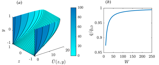
Figure 2: Base state velocity for a channel with $W=20$ for $G\sin(\beta)=40$. (b) Normalized local flow rate per unit width $\bar{q}$.

Figure 2(a) shows the base state velocity for a confined channel with $W=20$. The color scale presents the percentage drop in the velocity profile $\bar{U}(z,y)$ from the $1D$ Nusselt velocity profile $\bar{U}_{1D}(y)$ along the $y$-direction. Clearly, the base state is only affected in a small region near the side walls, in which the velocity is slowed down, while it retains the Nusselt film solution in most of the channel width. We approximate this region to be in the order of the mean film thickness $h_{m}$. This is expected since the side walls effect on the velocity is mainly controlled by the ratio between the film thickness and the channel width which is typically small, for example, for a relatively narrow channel of $W=20$, this ratio equals $0.05$.

Moreover, the local flow rate per unit width ($\bar{q}$) along the channel width $W$ is shown in figure 2(b). The values are normalised with the flow rate per unit width for an infinitely wide channel ($\bar{q}_{1D}$), which is in fact equals to $G\sin(\beta)/3$. The local flow rate does not experience a significant drop even for relatively narrow channels. For example, the flow rate is only decreased by $5\%$ compared to the 1D flow rate for a channel width of $W=25$. The local flow rate asymptotically reaches $\bar{q}_{1D}$ as the channel width increases. This is again because the effect of side walls on the flow is restricted to a thin region in the vicinity of the walls, while outside this region, the flow obeys the 2D Nusselt flow.

2.3 Linear stability analysis

The flow field variables $\boldsymbol{q}(x,y,z,t)=(u,v,w,p$) in addition to the interface variable $h(x,z,t)$ are expanded as a sum of the base flow and an infinitesimal perturbation as:

&q(x,y,z,t) = ¯q(y,z,t) + ϵ~q(x,y,z,t),
h(x,z,t) = 1 + ϵ~h(x,z,t).

Expansions in 2.8 are then substituted in the governing equations (1) and boundary conditions (2.3–2.5), which are then linearized for $\epsilon<<1$ leading to the linearized perturbation equations at $O(\epsilon)$ :

& ∂_x ~u + ∂_y ~v + ∂_z ~w = 0,
∂_t ~u + ¯U ∂_x ~u + ∂_y ¯U ~v + ∂_z ¯U ~w + ∂_x ~p - ∇^2 ~u = 0,
∂_t ~v + ¯U ∂_x ~v + ∂_y ~p - ∇^2 ~v = 0,
∂_t ~w + ¯U ∂_x ~w + ∂_z ~p - ∇