Discovery and origin of the radio emission from the multiple stellar system KQ Vel

Abstract

KQ Vel is a binary system composed of a slowly rotating magnetic Ap star with a companion of unknown nature. In this paper, we report the detection of its radio emission. We conducted a multi-frequency radio campaign using the ATCA interferometer (band-names: 16cm, 4cm, and 15mm). The target was detected in all bands. The most obvious explanation for the radio emission is that it originates in the magnetosphere of the Ap star, but this is shown unfeasible. The known stellar parameters of the Ap star enable us to exploit the scaling relationship for non-thermal gyro-synchrotron emission from early-type magnetic stars. This is a general relation demonstrating how radio emission from stars with centrifugal magnetospheres is supported by rotation. Using KQ Vel’s parameters the predicted radio luminosity is more than five orders of magnitudes lower than the measured one. The extremely long rotation period rules out the Ap star as the source of the observed radio emission. Other possible explanations for the radio emission from KQ Vel, involving its unknown companion, have been explored. A scenario that matches the observed features (i.e. radio luminosity and spectrum, correlation to X-rays) is a hierarchical stellar system, where the possible companion of the magnetic star is a close binary (possibly of RS CVn type) with at least one magnetically active late-type star. To be compatible with the total mass of the system, the last scenario places strong constraints on the orbital inclination of the KQ Vel stellar system.

1 Introduction

The magnetic field topology of early-type magnetic stars is commonly described by the simple yet highly successful Oblique Rotator Model (ORM, Babcock, 1949; Stibbs, 1950). In this model the magnetic field has a dipole dominated topology, with the magnetic axis misaligned with respect to the stellar rotation axis. The stellar magnetic field (typical polar strength at the kG level, e.g. Shultz et al., 2019b) induces anisotropic chemical distributions at the stellar photosphere, which are responsible for the observed variability (Krtička et al., 2007). The ORM explains the typical variability (photometric and spectroscopic) of such stars as a consequence of stellar rotation. First discovered by Landstreet & Borra (1978), such stars may also be surrounded by a large-scale magnetosphere, filled with ionized material continuously lost from the stellar surface via a weak radiatively driven wind (Babel, 1995, 1996).

The ability of the magnetosphere to sustain the confined plasma against gravitational infall depends on a combination of field strength, plasma mass, and rotational speed (Petit et al., 2013). Fast-rotating stars need strong magnetic fields to confine the centrifugally supported plasma to co-rotate with the star, leading to the formation of an extended Centrifugal Magnetosphere (CM). The average rotation period and polar magnetic field strength of the stars with CMs analyzed by Petit et al. (2013) are $P_{\mathrm{rot}}\approx 3$ days and $B_{\mathrm{p}}\approx 6000$ G. The size of the CM is quantified by the Alfvén radius ($R_{\mathrm{A}}$). The Alfvén radius is where the magnetic field strength becomes no longer able to confine the plasma, setting the extent of the magnetosphere. In order to form a CM, the Alfvén radius must be larger than the Kepler co-rotation radius ($R_{\mathrm{K}}$). The photometric and spectroscopic variability from the CM has been modeled by the Rigidly Rotating Magnetosphere (RRM) model (Townsend & Owocki, 2005; Townsend, 2008; Oksala et al., 2015; Krtička et al., 2022; Berry et al., 2022). Different observing diagnostic techniques have been taken into account to discriminate between CMs and Dynamical Magnetospheres (DM), where in the latter the plasma falls back to the star owing to gravity. In particular, the study of the H$\alpha$ emission features has been explained by the presence of Centrifugal BreakOut (CBO) events (Ud-Doula, Owocki & Townsend, 2008) continuously occurring within the CMs (Owocki et al., 2020; Shultz et al., 2020).

The magnetospheres of early-type magnetic stars are frequently sources of non-thermal radio emission produced by a population of relativistic electrons that, moving within the stellar magnetosphere, radiate in the radio regime via the incoherent gyro-synchrotron emission mechanism (Drake et al., 1987; Linsky, Drake & Bastian, 1992; Leone, Trigilio & Umana, 1994). Furthermore, a rapidly increasing number of early-type magnetic stars have also been discovered to be sources of strongly circularly polarized pulses (up to $\approx 100\%$) (Trigilio et al., 2000; Das, Chandra & Wade, 2018; Das et al., 2019a, b; Leto et al., 2019, 2020a, 2020b; Das et al., 2022), that are produced by the electron cyclotron maser coherent emission mechanism (Trigilio et al., 2000). This coherent emission process has been explained as stellar auroral radio emission (Trigilio et al., 2011), similar to the terrestrial auroral radio emission. Such coherent emission, originating above the magnetic polar caps, is intrinsically highly beamed, with the emission pattern mainly oriented perpendicular to the magnetic axis. The maser emission is then usually visible within a limited range of stellar rotational phases close to the nulls of the effective magnetic curve. In some cases the coherent emission is visible over a broad portion of stellar rotational phases. This depends on a favorable stellar geometry (Leto et al., 2020b) or on the adopted (very low, typically a few hundred MHz) observing frequency (Das & Chandra, 2021).

The gyro-synchrotron radio emission arising from the co-rotating magnetospheres of early-type magnetic stars is modulated by stellar rotation (Leone, 1991; Leone & Umana, 1993), with the amplitude of the radio emission variability being a function of the ORM geometry, behavior that was successfully modeled by Trigilio et al. (2004). In particular, stars showing large-amplitude magnetic curves are also characterized by the larger rotational variability of their radio emission, i.e. see the cases of CU Vir (HD 124224), HD 37479 ($\sigma$ Ori E), or HR 7355 (HD 182180) that are characterized by large magnetic (Oksala et al., 2010, 2012; Rivinius et al., 2010; Kochukhov et al, 2014) and radio rotational variability (Leto et al., 2006, 2012, 2017), and the case of $\rho$ Oph C (HD 147932) that is instead characterized by small-amplitude rotational variability of its radio emission (Leto et al., 2020b). Although exceptions exist, i.e. HR 5907 (HD 142184) has a small-amplitude magnetic curve (Grunhut et al., 2012) and a rotational variability of the radio emission (at $\nu\gtrapprox 20$ GHz) with amplitude which increase as the observing frequency increases (Leto et al., 2018).

Recently, it was empirically found that the radio luminosity for incoherent non-thermal radio emission from large-scale corotating magnetospheres is nearly proportional to the square of the ratio between the unsigned magnetic flux ($\Phi=B_{\mathrm{p}}R_{\ast}^{2}$, where $B_{\mathrm{p}}$ is the polar strength of the dipole-like magnetic field) and the stellar rotation period ($P_{\mathrm{rot}}$), $L_{\nu,\mathrm{rad}}\propto(\Phi/P_{\mathrm{rot}})^{2}$ (Leto et al., 2021; Shultz et al., 2022). The underling physical mechanism supporting this empirical relation are continuously occurring CBO events. In the case of a simple dipole-shaped magnetic field topology, the magnetic field strength ($B$) in the magnetic equatorial plane rapidly decreases outward ($B\propto r^{-3}$ as a function of the radial distance $r$). The centrifugal force acting on the co-rotating plasma breaks the magnetic field lines. The magnetospheric region where CBO occurs is located at a well defined radial distance, where the magnetic tension is no longer able to constrain the centrifugal force. The resulting reconnection of the magnetic fields drives the acceleration of the local electrons that power the radio emission (Owocki et al., 2022). The existence of this general relation opens a new era in the radio study of magnetic stars surrounded by stable stellar magnetospheres. In fact, the measurement of radio luminosity has proved to be a powerful tool for indirect estimation of some fundamental parameters of such stars.

In this paper we present new radio observations of KQ Vel, performed with the ATCA interferometer. KQ Vel is a multiple stellar system. The brightest component is a well studied magnetic Ap star (Bailey, Grunhut & Landstreet, 2015), whereas the nature of the companion is not yet clear. The detection of the radio emission of KQ Vel provides useful new information for advancing our comprehension of the nature of this enigmatic stellar system. The known properties of KQ Vel are summarized in Sec. 2. In Sec. 3 we describe how the radio measurements were performed and how these data have been analyzed. The possible magnetospheric origin of the radio emission from KQ Vel is discussed in Sec. 4. The scenario involving the radio emission arising from a possible degenerate companion is discussed in Sec. 5, where the cases for both thermal and non-thermal origins have been analyzed. In Sec. 6 the explanation of the radio emission observing features related to the possible existence of an active binary system has been also taken into account. The results of the analyses performed in this paper have been discussed in Sec. 7. In Sec. 8 we proposed our conclusions and possible further steps for the next investigations aimed to definitively unveil the nature of the KQ Vel stellar system.

2 Summary on KQ Vel

KQ Vel (HD 94660) is a magnetic bright (visual magnitude 6.11) Ap star of the southern hemisphere about $260$ Myr old (Kochukhov & Bagnulo, 2006). Based on the early data of the third release of the Gaia mission (Gaia Collaboration, 2021) (data confirmed by the Gaia third release; Gaia Collaboration, 2022), Bailer-Jones et al. (2021) estimates the photogeometric distances and locates KQ Vel at $160\pm 8$ pc from Earth, which is compatible with the distance reported by Hipparcos ($d=150\pm 20$ pc; van Leeuwen, 2007). The first measurement of the magnetic field of KQ Vel was reported by Borra & Landstreet (1975). In the ORM paradigm, the stellar rotation induces the variability of the projected magnetic field components integrated over the whole visible disk. In fact, the magnetic field measurements of KQ Vel have been used to estimate the stellar rotation period. In particular, this Ap star is a long-period slow rotator. The first estimation of its rotation period, which was performed using magnetic field measurements, was $P_{\mathrm{rot}}\approx 2700$ d. This period was obtained from the variation of the modulus of the mean magnetic field at the stellar surface (Landstreet & Mathys, 2000). This is in good accord with the period previously estimated by the photometric variability (Hensberge, 1993). The period estimation has since been refined using magnetic field measurements covering a wider temporal baseline by Landstreet, Bagnulo & Fossati (2014) ($P_{\mathrm{rot}}=2800\pm 250$ d). Finally, collecting new high sensitivity magnetic field measurements (typical errors a few tens of gauss), Giarrusso et al. (2022) both confirmed the above period and improved on its precision ($P_{\mathrm{rot}}=2830\pm 140$ d).

The measured upper limit of the projected rotational velocity ($v\sin i<2$ km s^-1) and the modeling of the magnetic field variability indicate that the stellar rotation axis of this magnetic Ap star is inclined by only a few degrees ($i_{\mathrm{rot}}\approx 16^{\circ}$) with respect to the line of sight (Bailey et al., 2015). Further, the measured effective magnetic field of KQ Vel is always with negative polarity, showing a small amplitude of rotational variability ($\approx 800$ G). This means that KQ Vel is characterized by an ORM geometry where the negative stellar magnetic pole is always visible. As a first-order approximation, the magnetic field topology of KQ Vel is described by a simple less tilted dipole (tilt angle with respect to the rotation axis $\beta\approx 30^{\circ}$) with a polar magnetic field strength $B_{\mathrm{p}}\approx 7500$ G (Bailey et al., 2015).

This magnetic Ap star is also a member of a multiple stellar system. The binary nature of KQ Vel was first reported by Mathys et al. (1997) revealing also that the orbital period is significantly shorter than the rotation period of the Ap star. Multi-epoch high-resolution spectra evidenced a clear radial velocity variation (amplitude $\approx 35$ km s^-1) of $\approx 840$ d (Bailey et al., 2015). Collecting a large number of additional spectra, the orbital period, the mass function, and other orbital parameters have been constrained by Mathys (2017). These orbital parameters are well in good agreement with values estimated by Giarrusso et al. (2022), the latter having slightly higher uncertainty.

High-quality visual spectra of KQ Vel did not evidence any clear spectral signatures able to characterize the nature of the companion of the bright magnetic Ap star (Bailey et al., 2015). On the other hand, KQ Vel is also a bright X-ray source whose origin cannot be simply related to the visible Ap star (Oskinova et al., 2020). To explain how the X-ray emission from KQ Vel originates, different scenarios involving the unknown companion have been proposed. Oskinova et al. (2020) considered various scenarios, including a possibility that the companion is a RS CVn-type binary consisting of late-type stars with high-level of coronal magnetic activity. This possibility was discarded because typical activity signs (e.g. CaII spectral lines) have not been reported in the literature. Finally, Oskinova et al. (2020) favored a scenario involving the presence of a hot shell surrounding a massive degenerate unseen companion (a propelling magnetic neutron star) as responsible for the observed X-ray emission. However, the detection of a faint infrared source close to the bright Ap star, with short-period (2.1 d) photometric variability, and of flares (Schöller et al., 2020) re-opened the possibility that the companion of the Ap star is a binary system composed of a pair of non-degenerate stars, with masses close to the mass of the Sun and characterized by solar-like magnetic activity able to explain the measured X-ray emission level.

3 Radio observations

The radio observations of KQ Vel were performed with the ATCA (Australia Telescope Compact Array) using the CABB wide-band backend, that allow observation of a frequency window $\approx$ 2 GHz wide. The source was observed during the $\approx 12.5$ hours of visibility above the horizon limit. We cyclically alternated three receivers: the first with central frequency band tuned to $\nu=2.1$ GHz (band name 16cm); the second that is able to acquire two simultaneous bands tuned to $\nu=5.5$ and $\nu=9$ GHz (band name 4cm); and the third (band name 16mm) with a setup that acquires two simultaneous contiguous bands tuned to $\nu=17$ and $\nu=19$ GHz. The available observing time (reduced for array setup and calibrations) allowed us to observe KQ Vel at six different hour angles, for each band, which was enough to properly sample the uv-plane using the ATCA interferometer which has a linear array design.

Table 1: Observing log. Array configuration 6B; Code: C3379.

Date	$<$UT$>$	$\nu$	Phase cal	Flux cal
		(GHz)
2020-Oct-20	22:30	2.1 / 5.5 / 9 / 17 / 19	$1104-445$	$1934-638$

The phase calibrator PKS $1104-445$ was observed at all selected bands. The source $1104-445$ is a standard ATCA calibrator, that is ideal to calibrate the phases of the complex visibilities of KQ Vel (distance from KQ Vel $3.38$ deg). Within each individual scan, the observations were performed by cyclically switching the pointing of the target (KQ Vel) and of the phase calibrator. Due to the time lost for phase calibrator observations, the effective time on source was about $150$ minutes per band.

The flux density scale was defined by observing the Seyfert Galaxy PKS $1934-638$, which is the standard primary calibrator for the ATCA, used also to calibrate the frequency-dependent receiver response (bandpass calibration). The flux density uncertainty of the flux calibrator $1934-638$ is below $0.2\%$ in all the observing bands. Details regarding the observations are summarized in Table 1.

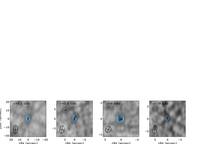
Figure 1: Maps performed at the sky position of KQ Vel at the indicated observing frequency. The light-blue contour levels are scaled in unit of the RMS of each map (values reported in Table 2); the lower level is fixed at $3\sigma$. The elliptical synthetic beams of the ATCA linear interferometer obtained using all the available observing scans are pictured in the left-bottom corner of each map.

The data have been edited and calibrated using the software package miriad, which is the standard for ATCA measurements. The bad data affected by strong RFI have been flagged (task blflag). The single observing scans performed at different hour angles allowed us to perform the cleaned maps (for all the observing bands) centered at the sky position of KQ Vel (tasks invert, clean, and restore). Cleaned maps (2000 iterations) were obtained at each observing frequency for both $I$ and $V$ Stokes parameters using the natural weighting. The Stokes $I$ parameter is always positive and is the measure of the total intensity of the electromagnetic wave, that is composed of the two opposite circularly polarized components with right (RCP) and left (LCP) rotation senses: Stokes $I=({\mathrm{RCP}}+\mathrm{LCP})/2$. The Stokes $V=({\mathrm{RCP}}-\mathrm{LCP})/2$ instead measures the intensity of the circularly polarized radiation and its sign is related to the dominant polarization state. The sign/orientation of the circularly polarized radiation follows the IAU/IEEE convention. That is, the polarization plane of the incoming right-handed circularly polarized radiation is seen to rotate counterclockwise. Conversely, the LCP circularly polarized radiation rotates clockwise.

Due to the need to flag channels and scans corrupted by strong RFI, the effective observing bandpass and integration time were reduced, with the consequent increase of map noise. The noise of the maps obtained in each band are listed in column 4 of Table 2. The measured map noise for the two bands available using the 4cm receiver was close (but worse) to the theoretical expected noises level ($\lessapprox 10$ $\mu$Jy/beam). In any case, the total intensity (Stokes $I$) radio emission of KQ Vel was clearly detected in both bands. The hard data flagging and the crowded field most significantly affected the noise level of the 16cm observations. The noise measured in the total intensity map is $\approx 30$ $\mu$Jy/beam, which is significantly higher than the expected value ($\approx 10$ $\mu$Jy/beam); however, the target was safely detected (Stokes $I$ only) well above the $5\sigma$ detection threshold. The noise measured in the map of Stokes $V$ performed at 2.1 GHz is $\lessapprox 20$ $\mu$Jy/beam. As expected, the noise measured in the Stokes $I$ map was significantly higher due to the large number of unpolarized bright sources present in the crowded field around KQ Vel.

Table 2: Measured radio fluxes and ATCA beams at each frequency.

$\nu$	S	$\pi_{\mathrm{c}}$	RMS	FWHM	PA
(GHz)	($\mu$Jy)		($\mu$Jy/beam)	(${}^{\prime\prime}\times^{\prime\prime}$)	(degree)
2.1	$201\pm 47$	$\lessapprox 14\%^{{\dagger}}$	28	$10.16\times 4.98~{}~{}$	$-4.91$
5.5	$86\pm 18$	$\lessapprox 14\%~{}~{}$	13	$4.29\times 2.28$	$-12.14$
9	$163\pm 32$	$\lessapprox 9\%~{}~{}$	15	$2.06\times 1.74$	$-24.30$
$18^{\ast}$	$94\pm 23$	$\lessapprox 20\%~{}~{}$	18	$1.43\times 0.65$	$-9.04$

• ^† Calculated using the noise measured on the Stokes $V$ map (20 $\mu$Jy).

• ^∗ Average of the two bands of the 15mm receiver.

At higher frequencies KQ Vel was not clearly detected in each single band available for the 15mm receiver. Hence, to improve the signal to noise level we combined the two bands centered at $\nu=17$ and $\nu=19$ GHz. After the averaging process, the central frequency is $\nu=18$ GHz and the corresponding map noise becomes comparable (or better) to the noise levels theoretically expected for the maps performed at the two single bands of the 15mm receiver ($\approx 20$ $\mu$Jy/beam). This enables us to report the detection ($5\sigma$ detection level) of KQ Vel at this high frequency.

The target is seen as a point-like source at each frequency, except at $\nu=9$ GHz. The radio maps performed at each observing frequency are shown in Fig. 1. The fluxes have been measured by fitting a bi-dimensional gaussian function at the sky position of KQ Vel, with the fit performed using the two-dimensional fitting tool implemented within the task imview (“gaussfit” button) of the casa package. Even if the source at 9 GHz seems slightly resolved (see Fig. 1), the deconvolution from the instrumental beam, computed by the bi-dimensional gaussian fitting procedure, is not able the resolve the source, reporting the message that the “source may be (only marginally) resolved in only one direction”. In any case, the faint flux level combined with the limited array spatial resolution prevents reliable clues on the morphology of this radio source.

The errors related to the measured flux densities of KQ Vel, in all bands, have been computed by adding in quadrature the noise of the maps (measured within regions far from background sources), the uncertainty related to the source fitting process, and 5% of the fluxes to take into account calibration errors. The measured fluxes of KQ Vel, with the corresponding errors, are listed in Table 2, where the map noise at each observing frequency and the corresponding upper limit of the circular polarization fraction ($\pi_{\mathrm{c}}=I/V$) have been also reported. The measured peak intensity at 9 GHz returned by the gaussian fit is $120\pm 20$ $\mu$Jy/beam; that, within the related uncertainties, is compatible with the integrated flux listed in Table 2. Note that, in case of a point-like source the peak intensity value coincides with the flux of the unresolved source integrated over the instrumental beam.

The radio spectrum of KQ Vel has a slightly negative spectral slope characterized by a spectral index of $-0.2\pm 0.2$. Finally, the data time series was split into two runs which were separately imaged to search for possible time variability. This process increases the noises of the maps, therefore the faint radio signal of this source prevents a reliable analysis performed over shorter time scales. Within these technical limitations, we did not detect significant time variability.

4 Magnetospheric radio emission

The average fluxes, reported in Table 2, scaled at the distance of KQ Vel (see Table 3) allows estimation of the radio spectral luminosity $L_{\nu,\mathrm{rad}}=4(\pm 2)\times 10^{15}$ erg s^-1 Hz^-1 at the mean frequency $<\nu>\approx 6.6$ GHz. To explain the origin of radio emission from KQ Vel, the most obvious scenario is to hypothesize that it arises from the magnetosphere of the bright early-type magnetic star.

The measured spectral index of the KQ Vel radio spectrum ($\alpha=-0.2\pm 0.2$) is compatible with the typical almost flat spectra of the non-thermal radio emission originating within the dipole dominated magnetospheres of early-type magnetic stars, as for example the strongly magnetized ($B_{\mathrm{p}}\approx 9.5$ kG; Shultz et al., 2019b) B2V star HR 7355 (HD 182180), whose rotationally averaged radio spectrum, covering a similar frequency range to that of the multi-frequency ATCA measurements of KQ Vel, is characterized by a spectral index $\alpha\approx-0.1$ (Leto et al., 2017).

In general, the flat spectrum behavior of the gyro-synchrotron radio emission of the early-type magnetic stars covers quite a large spectral range, roughly tuned in the range $\approx 1$–100 GHz (Leto et al., 2021). This is a consequence of the typical polar field strength of the sample of radio-loud stars ($\approx 1$–15 kG) analyzed by Leto et al. (2021). The observed spectral behavior of KQ Vel’s radio emission is compatible with the typical behavior of the magnetospheric radio emission of early-type magnetic stars, even if, on the basis of the ORM geometry and observed frequency range, KQ Vel is expected to have a small amplitude of radio emission rotational variability. In any case, the extremely long rotation period of this magnetic star ($P_{\mathrm{rot}}\approx 2800$ d) makes it impossible to detect any rotational modulation of its radio emission using current ATCA measurements. The geometry of KQ Vel is also not favorable for the detection of possible coherent emission from this magnetic star. In fact the stellar effective magnetic field does not invert sign (i.e., an absence of nulls), furthermore the ATCA observations are not tuned at a very low observing frequency. These unfavorable conditions were confirmed by the ATCA radio observations, which did not detect any evidence of circularly polarized radio emission from KQ Vel (see Table 2).

Table 3: Stellar parameters of KQ Vel.

$d$ (pc)	$160\pm 8$	Bailer-Jones et al. (2021)
$P_{\mathrm{rot}}$ (d)	$2830\pm 140$	Giarrusso et al. (2022)
$T_{\mathrm{eff}}$ (K)	$11300\pm 400$	Bailey et al. (2015)
$\log g$ (cgs)	$4.18\pm 0.20$	Bailey et al. (2015)
$M_{\ast}$ (M⊙)	$3.0\pm 0.2$	Bailey et al. (2015)
$L_{\ast}$ (L⊙)	$105\pm 20$	Bailey et al. (2015)
$R_{\ast}$ (R⊙)	$\approx 2.7$	this paper
$B_{\mathrm{p}}$ (kG)	$\approx 7.5$	Bailey et al. (2015)
$i_{\mathrm{rot}}$ (degree)	$\approx 16$	Bailey et al. (2015)
$\beta$ (degree)	$\approx 30$	Bailey et al. (2015)
Orbital parameters (Mathys, 2017)
$P_{\mathrm{orb}}$ (d)	$848.96\pm 0.13$
$T_{0}$ (HJD)	$2\,445\,628.6\pm 1.7$
$e$	$0.4476\pm 0.0049$
$V_{0}$ (km s-1)	$18.53\pm 0.06$
$\omega$ (degree)	$264.5\pm 0.8$
$K$ (km s-1)	$17.94\pm 0.11$
$f(M)$ (M⊙)	$0.3631\pm 0.0075$
$a\sin i$ (AU)	$1.25\pm 0.01$

The behavior of the radio emission from the early-type magnetic stars has been definitively quantified by the empirical scaling relationship between the radio spectral luminosity and the magnetic flux rate: $L_{\nu,\mathrm{rad}}{\propto}(\Phi/P_{\mathrm{rot}})^{2}={B_{\mathrm{p}}^{2}R_{\ast}^{4}}/{P_{\mathrm{rot}}^{2}}$, found by Leto et al. (2021) and confirmed by Shultz et al. (2022). This empirical relationship is the consequence of the physical mechanism supporting the non-thermal acceleration able to produce the electrons responsible for the magnetospheric radio emission of early-type magnetic stars. It was recently demonstrated by Owocki et al. (2022) that the power provided by centrifugal breakout events, continuously occurring within the stellar magnetosphere, is directly related to the power of the radio emission. From this point of view, the CBOs are non-random events. Breakouts occur continuously in a well-constrained magnetospheric region, where the resulting reconnection of the magnetic fields drives the acceleration of the local electrons. The CBO luminosity is related to the stellar parameters by the relation (Owocki et al., 2022):

$$L_{\mathrm{CBO}}=\frac{B_{\mathrm{p}}^{2}R_{\ast}^{3}}{P_{\mathrm{rot}}}\times W{\mathrm{~{}~{}(erg\,s^{-1}),}}$$

with $B_{\mathrm{p}}$ in gauss, $R_{\ast}$ in centimeters, and $P_{\mathrm{rot}}$ in seconds. In the above relation $W=2\pi R_{\ast}/P_{\mathrm{rot}}\sqrt{GM_{\ast}/R_{\ast}}$ is the dimensionless critical rotation parameter calculated as the ratio between the equatorial stellar velocity and the corresponding orbital velocity, defined by the gravitational law at the stellar equator ($G=6.67408\times 10^{-8}$ cm³ g^-1 s^-2 is the gravitational constant). Once the explicit relation of $W$ is substituted within the $L_{\mathrm{CBO}}$ definition, we find that $L_{\mathrm{CBO}}\propto{B_{\mathrm{p}}^{2}R_{\ast}^{4.5}M_{\ast}^{-0.5}}/{P_{\mathrm{rot}}^{2}}\propto L_{\nu,\mathrm{rad}}$, which in practice is almost the same relation empirically found, except for the term related to the mass, that in any case has negligible effect. The maximum possible value of $W$ is $W=1$, which, due to magnetic braking, would have to be at the beginning of the star’s life; however no magnetic star has ever been found with $W\gtrapprox 0.5$ (Shultz et al., 2019b). In fact, this parameter progressively decreases as the star loses angular momentum throughout its life (Keszthelyi et al., 2019, 2020).

Once the radio spectral luminosity ($L_{\nu,\mathrm{rad}}$) is integrated over a 100 GHz wide frequency range, in which the radio spectrum of a typical early-type magnetic star can be reasonably assumed to be flat (Leto et al., 2021), the efficiency of the CBO process supporting radio emission is $\approx 10^{-8}$ (Owocki et al., 2022). Therefore, the radio and the CBO luminosities are simply related by the relation (Owocki et al., 2022): $L_{\mathrm{rad}}\approx 10^{-8}L_{\mathrm{CBO}}$. In the case of a flat spectrum, the radio spectral luminosity is related to the power radiated over a frequency range $10^{11}$ Hz wide by the simple relation: $L_{\mathrm{rad}}{\mathrm{(erg\,s^{-1})}}=10^{11}{\mathrm{(Hz)}}\times L_{\nu,\mathrm{rad}}{\mathrm{(erg\,s^{-1}\,Hz^{-1})}}$. As evidenced by Leto et al. (2021), the gyro-synchrotron radio emission of the early type magnetic stars fade outside such a flat spectrum region.

The relationship reported above can also be generalized in cases of radio sources characterized by radio spectra covering frequency ranges narrower than 100 GHz, such as Jupiter’s non-thermal radio spectrum that is almost flat only below $\nu\lessapprox 1$ GHz (de Pater & Dunn, 2003), depending on the lower strength of the Jovian magnetic field ($\approx 4.17$ G; Connerney et al., 2018) compared to the case of the early-type magnetic stars. To compare the power provided by centrifugal breakout with the radio spectral luminosity, which is the unique observable available in cases of single-frequency radio measurements, the relationship is:

$$\frac{L_{\mathrm{CBO}}}{L_{\nu,\mathrm{rad}}}\approx 10^{19}\,\mathrm{Hz,}$$ (1)

which is derived from the relation $10^{-8}L_{\mathrm{CBO}}=10^{11}L_{\nu,\mathrm{rad}}$. This is formally similar to the Güdel-Benz relationship between X-ray luminosity and radio spectral luminosity characterizing a large range of stellar types with active coronae (Güdel & Benz, 1993; Benz & Güdel, 1994).

The magnetic, radio-loud early-type stars show the common behavior described by the above relationship, pictured in Fig. 2, where the two samples of radio detected stars collected by Leto et al. (2021) and by Shultz et al. (2022) are also shown. In Fig. 2, the cases of the non-thermal radio emission of the planet Jupiter and of the fully convective Ultra Cool Dwarf stars, already analyzed by Leto et al. (2021), are also shown. Note, that the non-thermal incoherent radio emission of the UCDs has been modeled taking into account the existence of a plasma source responsible for the surrounding stellar environment having a central symmetry (Ravi et al., 2011), like the case of the early-type magnetic stars.

Note that an explanation of the slight discrepancy of Jupiter with respect to the universal law reported in Fig. 2 was provided by Owocki et al. (2022). This is related to the non-central location within the Jovian magnetosphere of the plasma source: the volcanic moon Io that deposits plasma in an inhomogeneous and anisotropic way into the Io plasma torus.

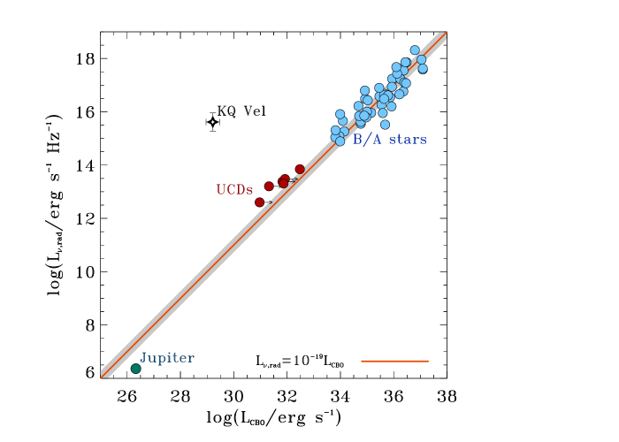
Figure 2: $L_{\nu,\mathrm{rad}}/L_{\mathrm{CBO}}$ diagram. The orange solid line represents the generalized scaling relationship (Owocki et al., 2022) between the radio spectral luminosity (erg s^-1 Hz^-1) and the power provided by centrifugal breakouts (erg s^-1); see text. This relation describes the common behavior of the non-thermal radio emission of stars and planets surrounded by large scale dipole-like co-rotating magnetospheres. The light-blue bullets represent the sample of early-type magnetic stars well studied at the radio regime (Leto et al., 2021; Shultz et al., 2022). The grey region around the orange line shows the statistical error of the B/A sample. The red bullets refer to the UCDs (the arrows refer to the cases with only estimates of the lower limit of the polar magnetic field strength). The green bullet locates the planet Jupiter. In the diagram the location of the early-type magnetic star member of the KQ Vel system is shown as a diamond symbol.

The main stellar parameters of the magnetic star of the KQ Vel system are reported in Table 3. The stellar radius is obtained scaling the value given by Bailey et al. (2015) at the distance of KQ Vel reported in the third release of the Gaia mission (Bailer-Jones et al., 2021). In practice, the stellar radius provided by Bailey et al. (2015) has been corrected by a factor 1.07, which is the ratio between the distance of KQ Vel provided by Gaia and the distance from Hipparcos ($160/150\approx 1.07$). This correction leaves the angular extension of the star unchanged, making all the other stellar parameters reliable. We note that the ORM parameters determined by Bailey et al. (2015) were derived purely from modeling the star’s magnetic field measurements, and as such are insensitive to any change in the assumed stellar radius. Using the stellar parameters listed in Table 3, the CBO power of the magnetic star is then $L_{\mathrm{CBO}}\approx 1.6\times 10^{29}$ erg s^-1, equivalent to $\log{L_{\mathrm{CBO}}}\approx 29.2$. The corresponding expected value of the radio luminosity of KQ Vel, estimated using the scaling relationship for radio emission summarized by Eq. 1, predicts a luminosity level of about $1.6\times 10^{10}$ erg s^-1 Hz^-1 ($\log{L_{\nu,\mathrm{rad}}}\approx 10.2$), which is substantially below the measured value of $\approx 4\times 10^{15}$ erg s^-1 Hz^-1, or $\log{L_{\nu,\mathrm{rad}}}\approx 15.6$. The location of KQ Vel in the ${L_{\nu,\mathrm{rad}}}/{L_{\mathrm{CBO}}}$ diagram is not in accordance with the prediction of Eq. 1 (see Fig. 2). Further, the above predicted magnetospheric spectral luminosity is even lower than KQ Vel’s photospheric contribution at $\nu=6.6$ GHz, which is about $2.1\times 10^{11}$ erg s^-1 Hz^-1, a value estimated assuming the stellar photosphere radiates like a black body: $L_{\nu}(T_{\mathrm{eff}})=4\pi R_{\ast}^{2}\times B_{\nu}(T_{\mathrm{eff}})$ erg s^-1 Hz^-1 (with the stellar radius given in centimeters). The spectral flux density of the black body in the Rayleigh-Jeans approximation is $B_{\nu}(T_{\mathrm{eff}})=2\pi k_{\mathrm{B}}T_{\mathrm{eff}}\frac{\nu^{2}}{c^{2}}$ erg s^-1 cm^-2 Hz^-1 (with $k_{\mathrm{B}}=1.38\times 10^{-16}$ erg K^-1 Boltzmann constant and $c=2.998\times 10^{10}$ cm s^-1 speed of the light).

The enormous discrepancy between the measured radio spectral luminosity and the value predicted by the universal law (Eq. 1), differing by $\approx 5$ dex, makes it hard to assign the radio emission from KQ Vel to being magnetospheric in origin from the magnetic Ap star member of the KQ Vel system. The very long stellar rotation period places the Kepler co-rotation radius for this Ap star at $R_{\mathrm{K}}\approx 450$ stellar radii (obtained equating the centrifugal and the gravitational accelerations: $R_{\mathrm{K}}(2\pi/P_{\mathrm{rot}})^{2}=GM_{\ast}/R_{\mathrm{K}}^{2}$, estimated using the parameters listed in Table 3). Such a high value of $R_{\mathrm{K}}$ is likely larger than the Alfvén radius. The values of $R_{\mathrm{A}}$ calculated for a large sample of early-type magnetic stars are typically lower than 100 stellar radii (Shultz et al., 2019b). The estimated upper limit for $R_{\mathrm{A}}$ has been derived for stars hotter than the Ap star component of KQ Vel, typically $T_{\mathrm{eff}}\gtrapprox 15$ kK (Shultz et al., 2019a). Using stellar parameters listed in Table 3, we obtain $R_{\mathrm{A}}\approx 106$ R_∗ adopting a wind mass-loss rate $\approx 10^{-11.9}$ M_⊙ yr^-1 using the recipe of Vink et al. (2001), or $R_{\mathrm{A}}\approx 415$ R_∗ using the mass-loss rate of $\approx 10^{-14.3}$ M_⊙ yr^-1 provided by Krtička (2014). Either of these values for $R_{\mathrm{A}}$ are lower than $R_{\mathrm{K}}$. Further, the adopted method overestimates the value of $R_{\mathrm{A}}$. In fact, the above analysis only takes into account the radiative wind, where the Alvén radius is simply related to the wind confinement parameter $\eta=B_{\mathrm{eq}}^{2}R_{\ast}^{2}/\dot{M}v_{\infty}$ (Ud-Doula & Owocki, 2002) by the simple relation $R_{\mathrm{A}}\propto\eta^{1/4}$ (Ud-Doula et al., 2008; Ud-Doula et al., 2014). The terminal wind velocity was assumed to be $v_{\infty}=500$ km s^-1, as adopted by Oskinova et al. (2020). But, as recently demonstrated (Leto et al., 2021), the centrifugal effects locate the Alfvén radius still closer to the star.

The condition $R_{\mathrm{A}}<R_{\mathrm{K}}$ is unfavorable for the generation of an extended CM (Petit et al., 2013), this also implies unfavorable conditions for triggering the CBO events able to supply the electrons necessary for the magnetospheric radio emission. The low radio emission level of KQ Vel predicted by the Eq. 1 indicates absence or negligible CBO events occurring within the magnetosphere of this slowly rotating magnetic star. This is in accordance with the absence of a CM surrounding the star. This is likely surrounded only by a low-density DM magnetosphere. The measured radio luminosity of KQ Vel is therefore totally inconsistent with the scaling relationship prediction. In fact no radio emission is expected due to the absence of a CM, further casting doubt on the Ap star as the origin of the radio emission.

5 Radio emission from a propelling NS

A magnetospheric origin for the measured KQ Vel radio emission was rejected in Sec 4. In the following sections we analyze other scenarios that may reveal where the radio emission comes from.

KQ Vel is characterized by a high X-ray emission level. The measured X-ray luminosity is $L_{\mathrm{X}}\approx 2\times 10^{30}$ erg s^-1. Model fitting of the X-ray spectrum of KQ Vel is compatible with thermal X-ray emission produced by hot electrons with a temperature higher than $T\approx 20$ MK and an emission measure $EM=n_{\mathrm{e}}^{2}V\approx 5\times 10^{52}$ cm^-3, or with a thermal component combined with non-thermal photons following a power-law distribution (Oskinova et al., 2020).

To explain the origin of the X-ray emission from KQ Vel, a scenario involving a degenerate objects was proposed by Oskinova et al. (2020). If the unknown companion of the early type magnetic star is a magnetized NS of about 1.5 M_⊙, the ionized material continuously lost by the radiative wind of the Ap star is gravitationally captured by the degenerate companion. In this case, the NS magnetic field forces the plasma to corotate giving rise to a “propeller effect” (Illarionov & Sunyaev, 1975), which can explain the origin of the hot emitting X-ray plasma.

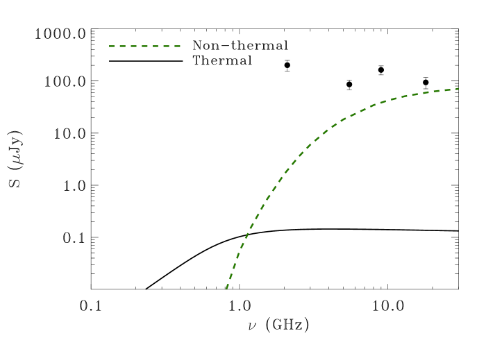
Figure 3: Thermal radio spectrum produced by the free-free emission mechanism arising from the hot ionized shell surrounding a propelling NS (solid line). The adopted model parameters are summarized in Sec. 5.1. The gyro-synchrotron radio spectrum of the NS magnetosphere (green dashed line) has been calculated assuming a spectral index $\delta=2$ for the power law of the non-thermal electron energy distribution and with a number density $n_{\mathrm{rel}}=n_{\mathrm{e}}/10$. The adopted source geometry is discussed in Sec. 5.2.

5.1 Thermal radio emission

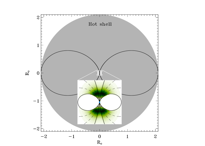
Figure 4: Synthetic brightness spatial distribution of the gyro-synchrotron radio emission (calculated at $\nu=30$ GHz) from the magnetosphere of the magnetic neutron star hypothesized to explain the X-ray emission from KQ Vel. The X-rays originate from a large thermal hot shell surrounding the propelling NS (grey region). The blue dot in the inset represents the magnetic NS (size not to scale). The zoomed area ($0.2\times 0.2$ R_⊙) shows that the brighter radio-emitting regions are mainly located at $\approx 0.04$ R_⊙ from the NS.

To reproduce the X-ray emission from KQ Vel, the hot ionized material is trapped within a shell, with inner radius $R_{\mathrm{in}}=0.1$ R_⊙ and outer radius $R_{\mathrm{ext}}=2.2$ R_⊙, centered on the propelling NS (see Oskinova et al., 2020 for details). Using the emission measure of KQ Vel, following the relation $n_{\mathrm{e}}=\sqrt{EM/V_{\mathrm{shell}}}$ (where $V_{\mathrm{shell}}$ is the volume of the shell), we derive an average electron density $n_{\mathrm{e}}\approx 1.8\times 10^{9}$ cm^-3 for this shell structure.

To check if the hot thermal plasma of the shell producing X-rays might also explain the measured radio emission from KQ Vel, we calculated the radio spectrum of this plasma shell. The model for the free-free emission from thermal electrons trapped within a spherical shell-like region was first proposed by Umana et al. (2008), successfully applied to reproduce the radio spectra of planetary nebulae (Cerrigone et al., 2008), and has also been used to study the radio emission from ultra compact HII regions (Leto et al., 2009).

Once the density and temperature of the thermal electrons (assumed to be homogenously spatially distributed) and the shell size have been assigned, the model is able to compute the radio emission produced by the free-free emission mechanism within a desired frequency range. The adopted model parameters coincide with the physical and geometrical parameters derived to explain the X-ray emission from KQ Vel. Those, for better clarity, are here summarized: the geometry of the source is a shell having internal and external radii of respectively 0.1 and 2.2 R_⊙; the radiating electrons (with a temperature equal to 20 MK) are assumed to be homogeneously spatially distributed, with an average density of $1.8\times 10^{9}$ cm^-3.

The radio spectrum of KQ Vel due to the thermal emission of the hot X-ray plasma is pictured in Fig. 3. The calculated emission level of the radio emission is too low ($\approx 3$ dex) to be able to reproduce the observed level. This demonstrates that the simple thermal emission of the ionized shell surrounding a NS cannot explain the origin of the radio emission from KQ Vel.

Table 4: Coronal parameters for the calculation of the radio spectrum using the core-halo model.

				Core				Halo
Radius of the active star		Size		Radius	$B$	$n_{\mathrm{rel}}$		Thickness	$B$	$n_{\mathrm{rel}}^{0}$
(R⊙)				(R∗)	(G)	(cm-3)		(R∗)	(G)	(cm-3)
		small		0.4	75	$2\times 10^{7}$		1	7	$3\times 10^{7}$
1		medium		0.68	220	$4\times 10^{5}$		3	10	$2\times 10^{6}$
		large		0.8	350	$1\times 10^{5}$		7	10	$7\times 10^{5}$
		small		0.25	95	$6\times 10^{6}$		0.5	7	$6\times 10^{6}$
2		medium		0.35	240	$3\times 10^{5}$		1	10	$1\times 10^{6}$
		large		0.45	400	$5\times 10^{4}$		3	10	$2\times 10^{5}$
		small		0.08	55	$1\times 10^{8}$		0.5	7	$7\times 10^{5}$
4		medium		0.15	210	$7\times 10^{5}$		1	10	$1\times 10^{5}$
		large		0.18	310	$2\times 10^{5}$		2	10	$5\times 10^{4}$

5.2 Non-thermal radio emission

The X-ray spectrum of KQ Vel is also compatible with the presence of a non-thermal component. This makes plausible the existence of non-thermal electrons within the hot plasma shell surrounding the magnetized NS. Following Oskinova et al. (2020), a dipole magnetic moment of $\mu=3\times 10^{30}$ G cm³ was derived for the propelling NS, typical for neutron stars, corresponding to a polar magnetic field strength of $6\times 10^{12}$ G, obtained using the simple dipole relation at the distance of 10 km, the typical radius of a neutron star. The corresponding average magnetic field strength, within the hot shell responsible for the X-ray emission, is $<B>\approx 0.4$ G. As discussed in the appendix of Oskinova et al. (2020), magnetic reconnection events can occur within the hot shell surrounding the NS, with consequent generation of a non-thermal electron tail having a density $\approx 10\%$ of the ambient hot thermal plasma. These relativistic electrons can power a non-thermal emission mechanism capable of producing detectable radio emission at the analyzed spectral range.

The harmonic numbers where the gyro-synchrotron emission mechanism efficiently works are $10\lessapprox\nu/\nu_{\mathrm{B}}\lessapprox 100$ (Dulk, 1985; Güdel, 2002), where $\nu_{\mathrm{B}}=2.8\times 10^{-3}(B/{\mathrm{G}})$ GHz is the local gyro-frequency. Within spatial regions characterized on the average by a magnetic field strength of about $0.4$ G, the harmonic number is higher than 100 already at $\nu\approx 0.1$ GHz. Hence, to produce an order of magnitude estimate of the non-thermal incoherent radio emission from the magnetosphere of the NS, we assume that all non-thermal electrons produced within the hot shell fall within spatial regions close to the NS, where the local magnetic field strength is high enough to produce significant radio emission falling within the spectral range analyzed in this paper.

The calculation of the radio spectrum arising from the NS magnetosphere has been performed using the procedures developed to calculate the radio spectrum from dipole-like magnetospheres surrounding early-type magnetic stars (Trigilio et al., 2004; Leto et al., 2006). The assumed energy spectrum of the relativistic electrons is a power law ($\propto E^{\delta}$), where the spectral index is fixed ($\delta=2$) and the low-energy cutoff is assumed to be 10 keV, whereas the high energy cutoff is fixed at 500 MeV. In any case, in the frequency range $\approx 1$–100 GHz, electrons with higher energy do not contribute to the non-thermal radio emission. The number density of the relativistic electrons is $n_{\mathrm{rel}}=0.1\times n_{\mathrm{e}}=1.8\times 10^{8}$ cm^-3. These non-thermal electrons homogeneously fill the magnetospheric regions crossed by the magnetic field lines that cross the magnetic equator at distances larger than $R_{\mathrm{in}}=0.1$ R_⊙.

The calculated spectrum is pictured in Fig. 3 using the dashed green line. In Fig. 4 the synthetic brightness spatial distribution of the radio emission from the magnetosphere of the NS is shown. It is clear that the radio emission would have to originate from regions located deep inside the propelling hot shell filled by thermal plasma. The absorption effects suffered by the radio radiation traversing the hot shell have been taken into account. The high-temperature thermal plasma of the hot shell is optically thin at the higher radio frequencies, whereas its absorption effects are not negligible at the lower frequencies. For example, at the lowest frequency analyzed here ($\nu=2.1$ GHz) the optical depth is $\tau_{\nu}\approx 0.23$, becoming larger than 1 at $\nu\lessapprox 1$ GHz. These frequency-dependent absorption effects significantly affect the shape of the calculated non-thermal radio spectrum. The comparison between measured and calculated radio emission shows that at higher frequencies the theoretical emission level is close to the observed one, whereas at the lower frequency side of the radio spectrum a clear discrepancy is evident.

The calculations performed here indicate that non-thermal radio emission is a favorable mechanism able to produce significant (detectable) radio emission at the higher radio frequencies analyzed. On the other hand, the hypothesized thermal plasma shell supporting the X-ray emission from KQ Vel has a not-negligible optical depth for the radio waves produced at lower frequencies, casting doubt on non-thermal emission from a propelling neutron star as the mechanism responsible for the measured radio emission. This shows that neither thermal nor non-thermal emission from a degenerate companion can reproduce KQ Vel’s radio spectrum.

6 Radio emission from a late type companion

Among the various scenarios explored by Oskinova et al. (2020) to explain the high X-ray emission level of KQ Vel, the possible existence of an active close binary orbiting around the Ap star was also considered. But, this hypothesis was discarded due to the lack of evidence of the typical spectral signatures of chromospheric magnetic activity (Bailey et al., 2015). On the other hand, the evidence of photometric variability and flares (Schöller et al., 2020) motivates reconsideration of the existence of a late type companion.

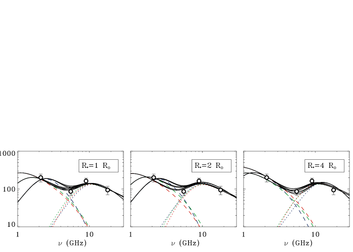
Figure 5: KQ Vel observed spectrum (open circles) with superimposed the radio spectra calculated using a core-halo model for the gyro-synchrotron emission mechanism from a stellar corona characterized by solar like magnetic activity. Different model parameters have been explored. The “halo” spectrum (dashed lines) arises from extended regions permeated by low strength magnetic field and dominating at the lower frequencies. The radio spectrum from the “core” (dotted lines) originates from a more compact region with higher magnetic field strength, that dominates at the higher frequency range. To distinguish the radio spectra calculated using coronal components of different sizes, the corresponding spectra have been displayed using different colors (the small, medium and large sizes are shown with blue, green, and red lines respectively). The total spectra obtained from combining each component have been pictured using the solid lines. Three different radii for the active star have been assumed for model calculations.

Chromospheric and coronal Solar-like magnetic activity is common in stars with deep convective zones. In the radio regime, coronal magnetic activity was recognized in the form of non-thermal radio emission characterized by stable emission levels and long-lasting active phases, with enhanced emission and flaring activity (Trigilio, Leto & Umana, 1998). Such non-thermal radio emission was mostly detected in fast-rotating stars, as confirmed by the correlation between the coronal radio emission level and the stellar rotation period (Mutel & Lestrade, 1985). This could be due to the dynamo mechanism amplified by rapid rotation. In particular, in the case of late-type stars that are components of close binaries, the tidal orbital interaction makes these stars rotate faster than single stars of similar spectral types. As an example, the basal emission level of the non-thermal coronal emission from the large binary $\alpha$ Cen A and B, the closest visible stars to Earth, is below the thermal chromospheric radio emission of both solar type stars (Trigilio et al., 2018). As expected, the stellar rotation periods are not affected by their large orbital separation, hence, the dynamo mechanism of the two stars does not seem to be amplified. KQ Vel evidenced photometric variability with a period of 2.1 days, much shorter than the 2800 d rotation period of the bright Ap star (Schöller et al., 2020). The observed periodicity is likely of rotational origin. This period is significantly shorter ($\approx 1$ dex) than the Sun’s period, or of the rotation periods of either component of the $\alpha$ Cen system. A higher level magnetic activity is thus expected, possibly supporting detectable non-thermal coronal radio emission.

To check if the measured radio spectrum of KQ Vel is compatible with non-thermal radio emission from a stellar corona, we calculated the gyro-synchrotron radio spectrum using a simplified model for the radio emission from the typical corona surrounding late-type stars. The model was developed to reproduce the radio spectra of the active magnetic star members of Algol-type binaries (Umana et al., 1993, 1999) and successfully used for the detailed analysis of the radio emission of an individual binary of RS CVn type (Trigilio et al., 2001). The model assumes the existence of a shell-like structure, the “halo”, which is a rough schematization of the extended stellar corona surrounding the late-type star, and of a spherical structure, the “core”, that represents a more compact region characterized by higher magnetic field strength with respect to the average value typical of the halo. This could correspond to an active region with an intense magnetic field and perhaps the base of a coronal loop filled by mildly relativistic non-thermal electrons. Following Umana et al. (1993), the non-thermal electrons are assumed to have a power-law energy distribution (adopted spectral index $\delta=2$), with energies in the range from 10 keV to 5 MeV. The “core” has been assumed to be homogeneously filled by non-thermal electrons; their density ($n_{\mathrm{rel}}$) is a free-parameter. In the case of the “halo”, the non thermal electron density was assumed to decrease with radial distance, following $n_{\mathrm{rel}}=n_{\mathrm{rel}}^{0}(R_{\ast/}r)^{2}$ (Umana et al., 1999). The corresponding electron density at the stellar surface ($n_{\mathrm{rel}}^{0}$) is a free-parameter of the model. The sizes of the two radio emitting regions are defined by the thickness of the “halo” and by the radius of the “core”. Both linear dimensions are also free-parameters. The magnetic field strengths of these regions have been assumed to have constant values and are free-parameters. Those are representative of the average field strengths within these coronal regions radiating at the radio regime for the gyro-synchrotron emission mechanism. The real magnetic field topology of the coronal regions is expected to be highly inhomogeneous, with the magnetic field vectors randomly oriented. It is then reasonable to assume an average magnetic field vector orientation of 45 degrees for both core and halo components (Umana et al., 1993).

The core-halo model requires the definition of six free-parameters for the radio spectrum calculation. The available multi-frequency radio measurements of KQ Vel are only four. This prevents applying any type of goodness of fit procedure to search for the optimal choice of the model parameters. We used the core-halo model only to test if plausible parameters exist, capable of providing a calculated spectrum that fairly matches the observed one. Further, we have no constraints regarding the real nature of the hypothesized late-type star. Consequently, we explored three possible stellar radii for this late-type star.

For the optimal choice of the model parameters, first we chose the radius of the late-type active stars, then arbitrarily fixed the linear sizes of the core and halo regions. Finally, we opportunely varied the other two parameters (magnetic field strength and non-thermal electron density) of each component to achieve a reasonable visual match between calculated and observed spectra. The adopted model solution search method is quite easy to perform; in fact each model component mainly dominates at a specific spectral range. In particular, the radio spectrum from the “core” dominates at the higher frequencies, whereas the “halo” spectrum dominates the low frequency range. Hence, the two model parameters of each specific component were varied independently. Once the visual match in the specific spectral range analyzed was considered satisfactory, the corresponding parameters were left fixed, to search for the better parameters of the other model component. Table 4 summarizes the model parameters that are able to reproduce both the shape and level of the observed radio emission from KQ Vel.

The radio spectra corresponding to each component of the core-halo model, for the assumed stellar radius, have been pictured in three panels of Fig. 5. The three different explored sizes of the “core” and “halo” are recognized by the adopted color code for the calculated radio spectrum (small sizes in blue; middle sizes in green; large sizes in red). The total spectrum has been obtained by combining the calculated spectrum corresponding to a combination of the free-parameters for a specific model component (core or halo) with all other spectra calculated using the parameters combinations of the other component. The total spectra obtained by combining all the core-halo model parameter are pictured in Fig. 5 superimposed with the multifrequency radio measurements. Inspection of the figure indicates that the present analysis cannot significantly constrain the free-parameters. The only worthwhile result is that the physical parameters used to calculate the gyro-synchrotron radio emission from a hypothetical late-type star are similar to the parameters used to reproduce the radio spectra of other well known late-type active star members of close binary systems (Umana et al., 1993, 1999; Trigilio et al., 2001). This supports the hypothesis that the observed radio emission from KQ Vel could originate from a late-type companion of the hot, bright, and magnetic Ap star.

7 Discussion

The analysis of the multi-frequency radio emission from KQ Vel showed that the measured level and spectral shape is compatible with a non-thermal radio spectrum from the corona of a magnetically active late type star. This is a further clue to explain the nature of the KQ Vel system. In fact, the study of KQ Vel performed in other spectral bands suggests the possible existence of a late type companion of the visible early type magnetic Ap star.

High resolution imaging in the near infrared H band, performed by the PIONIER (Precision Integrated-Optics Near-infrared Imaging ExpeRiment) instrument at the Very Large Telescope Interferometer (VLTI), detected an object fainter than the Ap star (difference of magnitudes $\approx 1.8$) and having an angular separation (18.72 mas) compatible with the orbital parameters of the system (Schöller et al., 2020). Further, the TESS (Transiting Exoplanet Survey Satellite) light curve showed clear photometric variability, compatible with a period of $\approx 2.1$ days, and two flare-like features (Schöller et al., 2020). On the other hand, the highly sensitive visible spectra of KQ Vel show spectral features related to the Ap star only (Bailey et al., 2015; Schöller et al., 2020). On the basis of the expected spectral line detection level, Schöller et al. (2020) concluded that the spectral signature of a couple of main sequence F8 type stars (or later) might be unseen. The fast stellar rotation typical of stars in close binary systems (with rotation periods of the order of a day) could explain the observed photometric variability.

The magnitudes of KQ Vel in the near- and mid- infrared bands are available in the Two Micron All Sky Survey (2MASS) (Cutri et al., 2003) and the Wide-field Infrared Survey Explorer (WISE) (Cutri et al., 2014) catalogues. The corresponding fluxes in these bands are shown in Fig. 6. For the magnitude to flux conversion, the zero-magnitude flux densities of the WISE bands listed by Wright et al. (2010) have been used; for the 2MASS bands the fluxes of the zero-magnitudes are instead listed by Cohen, Wheaton & Megeath (2003).

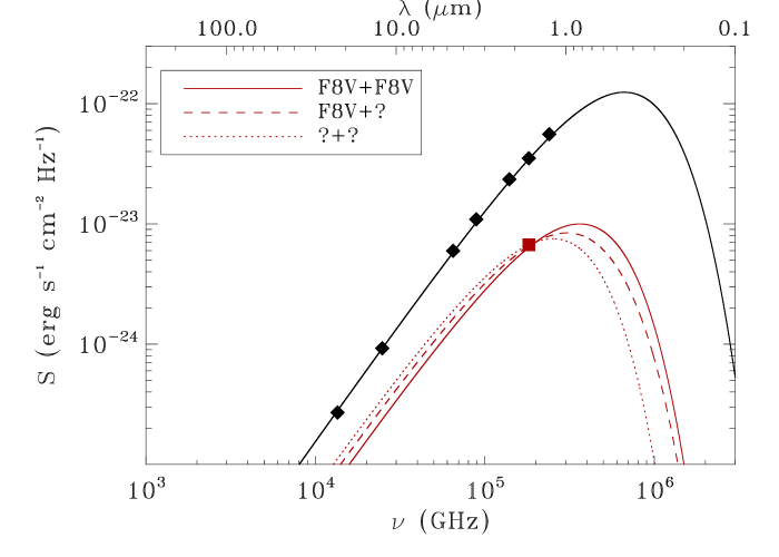
Figure 6: SED of KQ Vel. The black diamonds are the fluxes of the magnetic Ap star within the 2MASS and the WISE bands. The red square symbol refers to the flux in the H-band of the close faint object spatially resolved by the interferometric observations (Schöller et al., 2020). Refer to the text for explanation of the line types.

The spectral energy distribution of a black body at the temperature of KQ Vel has been superimposed on the infrared measurements (black solid line pictured in Fig. 6). The Stefan-Boltzman relation for the black-body radiation ($L=4\pi R^{2}\sigma T^{4}$) allows us to derive the stellar luminosity following the simple relation:

$$\frac{L_{\ast}}{{\mathrm{L}_{\odot}}}=\left(\frac{R_{\ast}}{{\mathrm{R}_{\odot}}}\right)^{2}\left(\frac{T_{\ast}}{{\mathrm{T}_{\odot}}}\right)^{4}$$

Using the stellar parameters listed in Table 3, the luminosity of the early-type magnetic star of the KQ Vel system is about 105 L_⊙. That is in good agreement with the value estimated by Bailey et al. (2015). The photospheric SEDs of typical Ap stars covering a wide spectral range, typically from the UV up to the NIR domain, have been reproduced using models of their stellar atmospheres (Shulyak, Ryabchikova & Kochukhov, 2013). In this paper, we adopted a simple black-body emission, which is only a rough approximation of the real SED which cannot be assumed to be valid at $\lambda<1$ $\mu$m. In any case, the analyzed NIR spectral domain and the high temperature of the Ap star analyzed here make the differences between the real SED and the black-body emission less dramatic.

Following the black-body emission framework, we also analyzed the faint IR companion of the bright Ap star. Using the typical temperatures and radii ($R_{\ast}\approx 1.3$ R_⊙; $T_{\mathrm{eff}}\approx 6200$ K) of a main sequence F8 star (Eker et al., 2018), the combined black body radiation of two F8 stars (as proposed by Schöller et al., 2020) are compatible with the H-band flux of the faint object seen in near infrared interferometry (red solid line pictured in Fig. 6). On the other hand, the nature of these stars cannot be unequivocally constrained. In fact, stellar parameters compatible with a sub-giant late-type star also provide black body spectra well in accordance with the H-band data (red dashed line of Fig. 6). The adopted stellar radius is $R_{\ast}=2$ R_⊙, equal to the value used in Sec. 6, whereas the temperature has been adapted to fit the H-band flux ($T_{\mathrm{eff}}=4300$ K). Also the black-body emission of two sub-giant late-type stars alone is enough to reach the measured H-band emission of the faint IR object (Fig. 6, red dotted line). The nature of this possible late-type companion is entirely uncertain, as the radius and the temperature are degenerate parameters with so few observational constraints. Hence, the stellar parameters used to calculate the black body spectrum have to be considered only a plausible combination able to fit the data, not the true parameters of a possible late-type companion of the Ap star. Further, the black body emission is only a rough approximation of the real stellar emission, which dramatically fails to reproduce the true atmospheric emission of the colder stars dominated by large absorption/emission bands produced by molecular complexes that survive within their cold stellar atmospheres. The above discussion can be considered only a rough semi-qualitative analysis. In Appendix A, the reliability of the above approach was tested in the case of two well studied close binaries composed of late type stars.

Following the clues that suggest the possible existence of a late-type star in the KQ Vel system, we also compared the X-ray and radio emission levels of KQ Vel with those typical of late-type stars. In fact, the radio and X-ray emission of late-type stars characterized by Solar-like magnetic activity have a well known and fairly stable behavior. The measured radio luminosity of KQ Vel is $L_{\nu,{\mathrm{rad}}}\approx 10^{15.6}$ erg s^-1 Hz^-1 and this is compatible with the typical radio luminosity (measured at 5 GHz) of the RS CVn active binaries, that is $L_{\nu,{\mathrm{rad}}}=10^{16\pm 1.5}$ erg s^-1 Hz^-1 (Drake et al., 1989). KQ Vel is also an X-ray source with an X-ray luminosity $L_{\mathrm{X}}\approx 10^{30.3}$ erg s^-1, which is in good accord with typical X-ray luminosities of magnetically active close binary systems: $L_{\mathrm{X}}=10^{30.5\pm 1.7}$ erg s^-1 (Drake, Simon & Linsky, 1989, 1992). Further, the radio and the X-ray luminosities of stars surrounded by active coronae are also correlated, as expressed with the empirical Güdel-Benz relationship (Güdel & Benz, 1993; Benz & Güdel, 1994), which for the chromospherically active stars also holds for coherent radio emission (Vedantham et al., 2022). In particular, in the case of active binaries (i.e. RS CVn type) their radio and X-ray properties follow the relation $L_{\mathrm{X}}/L_{\nu,{\mathrm{rad}}}=10^{14.7\pm 0.5}$ Hz (Benz & Güdel, 1994). Interestingly, in the case of KQ Vel the ratio of its radio and X-ray luminosities is exactly $L_{\mathrm{X}}/L_{\nu,{\mathrm{rad}}}\approx 10^{14.7}$ Hz.

The comparison between the X-ray and radio luminosities of the early-type magnetic stars is largely unexplored. The ratio $L_{\mathrm{X}}/L_{\mathrm{\nu,rad}}$ is available in the literature only for a few hot magnetic stars. Some B/A-type magnetic stars have $L_{\mathrm{X}}/L_{\mathrm{\nu,rad}}\approx 10^{12-14}$ Hz (Leto et al., 2017, 2018, 2020a; Robrade et al., 2018), which suggests that the X-ray/radio luminosity ratio of the hot magnetic stars deviates from the GB relation. This is likely due to the plasma processes occurring within the magnetospheres of the early type magnetic stars, which differ from those supporting the radio and X-ray emission from the coronae of the active stars. Extending to the case of KQ Vel the X-ray/radio behavior observed in the few early-type magnetic stars having measured X-ray/radio luminosities ratios, and using the spectral radio luminosity theoretically expected of the magnetic Ap star ($\approx 1.6\times 10^{10}$ erg s^-1 Hz^-1, see Sec. 4), we estimate an X-ray luminosity in the range $\approx 10^{22.2}$–$10^{24.2}$ erg s^-1, which is many order of magnitudes lower that the measured value ($L_{\mathrm{X}}\approx 10^{30.3}$ erg s^-1). Therefore, the possible contribution from the magnetic early-type star to the measured luminosity ratio of KQ Vel is likely negligible.

The radio and X-ray properties of KQ Vel seem to be well in agreement with typical behavior of close binary systems characterized by Solar-like magnetic activity. On the other hand, the typical spectral signatures of the chromospheric activity of late-type stars are the CaII H and K lines observed in emission. The absence of this signature within the visual spectra of the classical magnetic activity indicators (Bailey et al., 2015), the core of the CaII H ($\lambda=3968.469$ Å) and K ($\lambda=3933.663$ Å) lines observed in emission, suggests that this hypothetical late-type star could have a “weak” or “moderate” (Strassmeier et al., 1988) chromospherical magnetic activity.

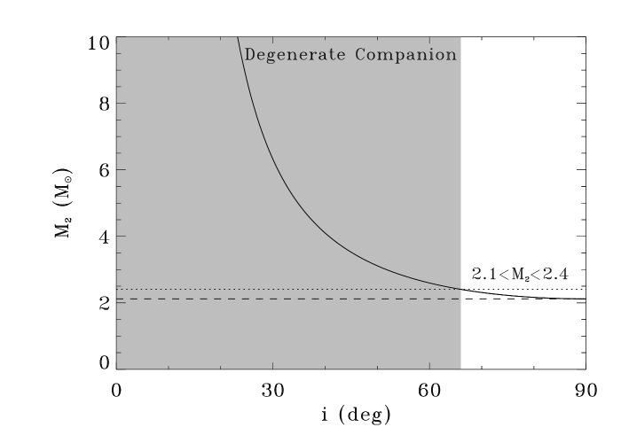
Figure 7: Mass of the faint companion of the Ap star as a function of the orbital plane inclination. The solid line shows the real solutions obtained by numerically solving the Eq. 2. The dashed line refers to the minimum mass compatible with the boundary geometric condition corresponding to the orbital plane aligned with the line of sight. The dotted line refers to the mass value compatible with the total mass of a close binary composed of two main sequence F8 type stars (see text). These masses define the range of allowed total mass of a binary system composed of non-evolved stars. The dashed area is pictured only to highlight those geometrical conditions of the orbital plane that are not compatible with the masses of normal stars. More massive stars provide detectable signatures in the visible spectra. As discussed in the text, a more massive companion should be a degenerate objet.

7.1 Considerations on the masses and the inclinations

KQ Vel is likely a hierarchical triple system, where the faint companion of the early-type magnetic star could be a close active binary system. But, the nature of this close binary is basically unknown. The orbital parameters obtained by fitting the measured radial velocity curve of the Ap star (Mathys, 2017), the visible member of the KQ Vel system, places strong constraints on the total mass of the system. In particular, the orbital inclination ($i$) plays a key role to estimate indirectly the mass of the companion ($i$ is the angle between the orbital plane and the plane tangent to the celestial sphere).

In the case of a single line spectroscopic binary system, the mass of the unseen component can be constrained by the binary mass function. The mass function is derived from Kepler’s third law and relates the mass of the star to orbital information, the mass of the unseen star, and the inclination $i$ of the orbital plane. Therefore, the total mass of the unseen companion of the KQ Vel system can be calculated as a function of the orbital plane inclination using the explicit relation of the mass function:

$$f(M)=\frac{M_{2}^{3}\sin^{3}i}{(M_{1}+M_{2})^{2}},$$ (2)

where the adopted value of the mass function (Mathys, 2017) is reported in Table 3. Assuming $M_{1}=3$ M_⊙ (the mass of the Ap star given by Bailey et al., 2015), the corresponding values of $M_{2}$ are shown in Fig. 7 as a function of the inclination $i$.

The lower limit mass ($M_{2}=2.1$ M_⊙) is defined by the geometrical condition of the line of sight lying in the orbital plane ($i=90^{\circ}$). As previously discussed, to satisfy all the observational constraints, the spectral types of the close binary members cannot be earlier than F8V (Schöller et al., 2020). The typical mass of an F8V type star is $M_{\ast}\approx 1.2$ M_⊙ (Eker et al., 2018). As a consequence, the upper limit of the total mass of the close binary is $\approx 2.4$ M_⊙. Hence the total mass of the secondary lies in the narrow range $2.1\lessapprox M_{2}\lessapprox 2.4$. On the other hand, the $M_{2}$ upper limit indirectly constrains the lower limit of the orbital inclination to $i\approx 65^{\circ}$. Therefore, if the inclination $i$ of the KQ Vel orbital plane were less than $\approx 65^{\circ}$, the corresponding total mass of the secondary component must be greater than 2.4 M_⊙ and consequently the non-degenerate members of the hypothesized close binary are expected to be too bright for their emission level to be compatible with the measured H band magnitude (Schöller et al., 2020). Therefore, the geometrical condition $i\lessapprox 65^{\circ}$ would require the existence of a degenerate object possessing a large fraction of the mass of the system to satisfy the orbital parameters of the visible Ap star.

The eccentric orbit of KQ Vel suggests that the distance between the members of the system is expected to be widely variable as a function of their orbital motion around the common center of mass. Note that, only the orbit of the visible star is known. The projected semi-major axis of the orbit of the visible star is 1.25 AU, listed in Table 3, corresponding to $\approx 100$ R_∗. Note that this is comparable to the Alfvén radius of the magnetic star (see Sec. 4). This can be also used to provide a rough estimation of the maximum orbital separation between the stellar components, about the major axis length ($\approx 2.5$ AU). At the distance of KQ Vel this is about 15.65 mas. The above rough estimation is close to the separation of 18.72 mas of the faint IR object measured by Schöller et al. (2020) using the Very Large Telescope Interferometer. When the members of the system are closer, i.e. at the distance $\approx 100$ R_∗, the magnetic field strength of the bright magnetic star is $\approx 7.5$ mG, obtained using the inverse cube law that describes a simple dipole with polar strength $B_{\mathrm{p}}\approx 7.5$ kG (Bailey et al., 2015). Hence the magnetic field strength in the spatial region where the unknown companion orbits is not negligible, furthermore, this is also expected to be strongly variable as the stars revolve around the center of mass along their eccentric orbits.

The orbital position of the magnetic early type star during the ATCA radio observations can be calculated using the ephemeris (Mathys, 2017) listed in Table 3. The radial velocity curve of KQ Vel, pictured in the top panel of Fig. 8, has been calculated using the orbital parameters provided by Mathys (2017). The calculation has been performed using the procedure helio_rv enabled within the idl data language, which returns the heliocentric radial velocity of a spectroscopic binary with known orbital parameters. The orbital phase of the magnetic star at the time the ATCA observations were performed is indicated by the vertical dashed line in Fig. 8.

The distance between the components of the KQ Vel stellar system is expected to be change substantially as they orbit around the common center of mass. The distance can be estimated by adding the radial distances ($r$) of the components from the focus of the ellipse where the common center of mass is located. The polar equation of the orbit of each component is:

$$r_{\mathrm{i}}=\frac{a_{\mathrm{i}}(1-e^{2})}{1+e\cos\theta},$$

where $\theta$ is the polar angle with the origin coinciding with the periastron. Both stars orbit around the common center of mass with the same eccentricity $e$, listed in Table 3. The semi-major axis of the unseen component can be derived by using the definition of center of mass: $a_{2}=a_{1}\times M_{1}/M_{2}$, where $M_{2}$ is constrained in the range 2.1–2.4 M_⊙, as discussed above. The distance $r=r_{1}+r_{2}$ between the components of the KQ Vel system as a function of the orbital phase is reported in the bottom panel of Fig. 8. The two almost indistinguishable lines refer to the two orbital inclination angles taken into account ($i=90^{\circ}$ and $i=65^{\circ}$).

The widely variable distance between the components of the KQ Vel system (range $\approx 130$–360 R_∗, lower limit close to the minimum component separation roughly estimated above) implies that it is likely to expect strongly variable magnetic interaction as a function of orbital position. Further, as suggested by the behavior at the low frequency side of the simulated spectra, pictured in Fig. 5, the size of the largest coronal component contributing to radio emission cannot be constrained by the radio measurements reported here (i.e. high sensitivity measurements at frequencies close to or lower than $\approx 1$ GHz might be helpful). If the observed radio emission originates from the magnetic corona of a late-type star, magnetospheric interaction may also affect the physical mechanisms able to produce non-thermal electron acceleration. This is only a speculative hypothesis; long-term monitoring of KQ Vel at the radio regime could be useful to confirm or refute the idea.

Finally, the age of the KQ Vel system (260 Myr) puts strong constraints on the nature of the late-type stars of the active close binary, hypothesized to be unknown companion to the bright Ap star. These cannot be evolved stars. The close binary is likely composed of two solar-like young stars in close orbit, like the case of $\sigma^{2}$ CrB. This is a young close binary, about 10 Myr old (Strassmeier & Rice, 2003), of RS CVn type. This is a well studied active binary composed of two main sequence F9V and G0V dwarf stars (see Appendix A.1 for additional details regarding $\sigma^{2}$ CrB).

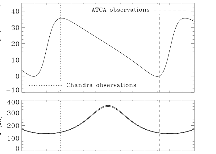
Figure 8: Top panel: radial velocity curve of the bright Ap star member of the KQ Vel system. The adopted orbital parameters are listed in Table 3. The vertical dashed line located the orbital phase when the ATCA observations were performed. Bottom panel: distance between the components as a function of the orbital phase.

It is worth noting that the rotation axis of the magnetic Ap star, i.e. the dominant member in the visible domain of the KQ Vel system, is tilted by only $\approx 16^{\circ}$ with respect to the line of sight. It follows, that in the case of large inclination of the orbital plane, the axial tilt between the rotation and the orbital axes (obliquity) is consequently expected to be large. The obliquity upper limit is $\approx 74^{\circ}$, in the case of the orbital plane being aligned with the line of sight ($i=90^{\circ}$). It follows, that in this case limit the Ap star revolves around the center of mass with its rotation axis almost contained within the orbital plane, this would be a really strange configuration.

7.2 Revisiting the neutron star companion scenario

The lower limit mass (2.1 M_⊙, see previous section) of the companion to the Ap star in the KQ Vel system is compatible with the possible presence of a compact object, such as e.g. a NS (Bailey et al., 2015). A NS companion can accrete matter from the wind sprayed out by the magnetic Ap star. In the case of a magnetized NS, the accretion of matter could also be a possible source of synchrotron radio emission. The accreting NS scenario has been considered by Oskinova et al. (2020) to explain the X-ray emission of KQ Vel, but ruled out above because the very low ambient plasma density predicts an X-ray emission level three orders of magnitudes lower than the measured X-ray luminosity.

The possible effects induced by the magnetosphere of the Ap star depend on the component separation, which is a function of the orbital phase. The measurements of the X-ray emission from KQ Vel have been performed by the Chandra X-ray telescope on 2016-Aug-20 (mean UT time about 11:00). The orbital phase when the X-ray measurements was performed is marked in Fig. 8 by the vertical dotted line, which corresponds to a distance between the components of $\approx 148$ R_∗. As discussed in Sec. 4, the magnetic Ap star is the source of a weak wind; two recipes have been taken into account to estimate its properties. Using the two different values of the wind mass loss rates adopted in this paper, we estimated the ambient density where the hypothesized NS is located at the epoch of the X-ray measurement. In stars with centrifugal magnetospheres accumulation of matter is expected within their magnetospheres. But in cases of dynamical magnetospheres, which is the case we’re dealing with (see Sec. 4), the accumulation of plasma is balanced by the gravitational infall, making reasonable to roughly assume the mass flux inside the magnetosphere coinciding with the flux of mass lost from the whole stellar surface due to the wind. In the case of a lower wind mass loss rate ($\dot{M}\approx 10^{-14.3}$ M_⊙ yr^-1), the corresponding Alfvén radius ($R_{\mathrm{A}}\approx 415$ R_∗) is larger that the component separation ($r\approx 148$ R_∗). Making the simplest assumption of a density profile $n\propto\dot{M}/(4\pi v_{\infty}r^{2})$, which is justified by the condition of dynamical magnetosphere, the ambient electron density $n_{\mathrm{e}}\approx 0.39$ cm^-3 was derived. The other wind regime taken into account in this paper is $\dot{M}\approx 10^{-11.9}$ M_⊙ yr^-1, which is able to open the magnetosphere at $R_{\mathrm{A}}\approx 106$ R_∗. The above value of the Alfvén radius is lower than the component separation. For the local electron density calculation, we crudely estimate the mass lost from the two polar caps where the magnetic field lines are assumed to be open (Ud-Doula & Owocki, 2002; Ud-Doula et al., 2008; Petit et al., 2017). To do this, we calculate the fraction of the stellar surface where the wind can freely propagate. This is the ratio between the polar caps area calculated using the latitude where the last closed magnetic field line, assumed to be a simple dipole, crosses the stellar surface, and the total stellar surface. In the case of $R_{\mathrm{A}}=106$ R_∗ and $R_{\ast}=2.7$ R_⊙, the fraction is $\approx 0.5$%, the corresponding actual wind mass loss rate is $\dot{M}_{\mathrm{act}}\approx 10^{-14.2}$ M_⊙ yr^-1, which corresponds to a local ambient electron density of about 0.46 cm^-3 at the the distance of 148 R_∗. We emphasize that the two different mass loss recipes, when magnetic confinement is accounted for, result in similar densities at the companion’s position.

Adopting the same parameters as in Oskinova et al. (2020), and assuming a spherical wind density radial profile, the corresponding ambient electron density is $n_{\mathrm{e}}\approx 1.6$ cm^-3, which is higher than both values estimated in this paper. Therefore, the wind parameters given in this paper provide a more stringent condition regarding the capability of an hypothetical accreting NS to support the observed X-ray luminosity. The inability to reproduce one (the X-rays) of the two observables (X-rays and radio) analyzed in this paper convinced us to not investigate further the accreting NS scenario.

8 Summary and conclusions

In this paper the multi-frequency radio detection, performed by the ATCA interferometer, of the KQ Vel multiple stellar system is reported. These new radio measurements have been used to put constraints on the nature of this enigmatic stellar system. When observed at visible wavelengths high-resolution spectra of KQ Vel show only evidence of an early-type magnetic star (Bailey et al., 2015). This long-period magnetic star ($P_{\mathrm{rot}}=2830$ d; Giarrusso et al., 2022) is a member of a high eccentricity multiple system as directly evidenced by the measured radial velocities (Mathys, 2017), but no evidence of the companion is seen at visible wavelengths, hence its nature remains unclear. The only direct measurement of the companion’s brightness was performed at the infrared domain with interferometric observations reported by Schöller et al. (2020).

The stellar parameters of the visible magnetic star belonging to the KQ Vel system are well known, which enables us to check the possible magnetospheric origin of the measured radio emission. Comparing the radio luminosity of KQ Vel with the luminosity level predicted by the universal law of radio emission from well ordered and stable co-rotating magnetospheres, that was empirically discovered by Leto et al. (2021), confirmed by Shultz et al. (2022), and then theoretically supported by Owocki et al. (2022), we found that the observations are dramatically above ($\approx 5$ dex) the theoretical prediction, because the star is an extremely slow rotator. We therefore reasonably ruled out non-thermal radio emission from the magnetosphere of the visible early-type magnetic star as a possible origin of the measured radio emission.

KQ Vel is also a bright X-ray source. To explain the X-ray emission level and spectrum, Oskinova et al. (2020) proposed a scenario where the X-ray emission originates from a hot plasma shell surrounding an unseen degenerate magnetic companion, probably a neutron star. We analyzed if the above scenario, able to explain the X-ray emission, is also able to explain the origin of the radio emission. The radio emission level of the X-ray emitting thermal plasma (given by the thermal bremsstrahlung emission mechanism) is too low to explain the measured radio emission. On the other hand, a significant fraction of the hot plasma gravitationally captured by the neutron star might be accelerated to relativistic energies. We also checked if the non-thermal electrons falling inside the deep magnetospheric regions close to a magnetic degenerate object are able to produce detectable radio emission by the gyro-synchrotron emission mechanism. The calculated theoretical emission level is close to the observed one at the higher frequencies. However, we found that the low frequency side of the calculated radio spectrum suffers significantly from frequency-dependent absorption effects produced by the thermal plasma envelope (responsible for the X-rays) surrounding the magnetospheric regions responsible for the non-thermal radio emission. Therefore neither thermal nor non-thermal emission from a propelling neutron star are consistent with the properties of KQ Vel’s radio spectrum.

Oskinova et al. (2020) also considered the possibility of an active binary star companion. This was corroborated by the discovery of periodic photometric variability, with a period of about 2.1 days, evidence of flares, and the interferometric detection of a companion star in the right magnitude range for a solar-type object. This suggests the possible existence of a companion with Solar-like magnetic activity (Schöller et al., 2020), that might be responsible for the observed photometric behavior. Hence, KQ Vel could be a hierarchical multiple stellar system hosting a late-type star (or stars) with an extended corona sustained by a large-scale magnetic field generated by the dynamo mechanism acting within the deep convective layers below the stellar photosphere (i.e. the active members of close binaries like the RS CVn systems). In principle, the coronal magnetic activity of such a possible late-type companion might explain both the X-ray and radio emission of KQ Vel. Further, the measured radio and X-ray luminosity ratio is well in accordance with the Güdel-Benz law prediction in the case of an RS CVn system. We calculated the non-thermal radio spectrum arising from an extended stellar corona. For a hypothesized active member of the KQ Vel system, we adopted plausible stellar parameters that are compatibile with those used to reproduce the observed radio spectra of known active binary systems well studied at radio wavelengths. Using model parameters that are canonical for active close binary systems, the calculated radio spectrum, scaled at the distance of KQ Vel, matches the observed one.

The scenario where the KQ Vel system hosts a star characterized by Solar-like magnetic activity seems preferred. On the other hand, the mass of the early-type magnetic star and its orbital parameters places strong constraints on the mass of the unknown companion. In fact, the minimum mass of the companion that is compatible with the mass function of KQ Vel is higher than 2.1 M_⊙, which is in accordance with the total mass of typical RV CVn active binary system. But the inclination of the orbital plane of the KQ Vel system is unknown. The above reported lower limit of the mass of the unseen companion was obtained in the case of the orbital plane perfectly aligned with the line of sight. If the orbital plane has a smaller inclination (i.e. the orbit view becomes close to the face-on view), the mass of the companion required to explain the observed radial velocity curve increases. If the required mass of the unknown companion of the KQ Vel system needs to increase, the star will be consequently brighter. Schöller et al. (2020) estimated that the spectral signatures of a couple of normal F8 type stars are undetectable in the high-sensitivity visual spectra of KQ Vel. The above condition definitively fixes the upper limit of the total mass of the KQ Vel companion in the case of normal main sequence stars. To take into account possible lower inclination of the orbital plane, the existence of a degenerate object is mandatory. The eccentric orbit implies that along its orbital motion the unseen companion meets widely variable conditions (i.e. the magnetic field strength and the plasma density provided by the magnetic Ap star). Such variable conditions may affect the X-ray emission and likewise the radio emission. This motivates interferometric monitoring, which together with existing RVs would constrain the inclination of the orbit and therefore provide a definitive test. The unknown component of the KQ Vel system could be an exotic close binary consisting of a degenerate object and a late-type star (Oskinova et al., 2020), possibly characterized by enhanced solar-like magnetic activity that explains the radio and X-ray observing features.

The measured radio flux density of KQ Vel is quite low ($\approx 100$ $\mu$Jy), this makes it hard to study the radio source morphology and also to reveal possible radio emission variability related to the orbital position. Indeed, it is well known that the non-thermal radio emission of active binary systems is strongly variable. Future high-sensitivity radio measurements with higher spatial resolution, performed using the forthcoming SKA or its precursors (MeerKAT, ASKAP, or ngVLA), will be crucial for definitively revealing the nature of the enigmatic KQ Vel stellar system.

Data availability

The data underlying this article are available within the body of the paper and within its tables.

Appendix A The IR SEDs of two close binaries

The black-body spectrum is only a rough approximation of the true spectral energy distribution of the photospheric emission of stars, in particular late type stars. This approximation has been adopted here only to check if the expected emission from stars belonging to close binary systems classified as RS CVn type, that also have well known sizes and temperatures, might be considered fairly in accordance with measurements in the infra-red spectral domain. In the following, two well studied close binary of RS CVn type have been taken into account. The two selected binaries have almost similar total masses (2.2 and 2.4 M_⊙, compatible with the mass constraint of the secondary component of the KQ Vel system), but with different evolutionary stages. The young $\sigma^{2}$ CrB is composed of a pair of similar dwarf stars, whereas TY Pyx is composed of two sub-giant stars of the same spectral type.

A.1 The young active binary $\sigma^{2}$ CrB

Figure 9: SEDs of two well studied close binaries of RS CVn type. The black diamonds are the fluxes of $\sigma^{2}$ CrB and TY Pyx within the 2MASS, WISE, IRAS, and AKARI bands. Top panel: SED of $\sigma^{2}$ CrB, the solid line is the combined black body emissions of two F9V and G0V main sequence stars at the distance of $\sigma^{2}$ CrB. Bottom panel: SED of TY Pyx, the solid line is the combined black body emissions of two sub-giant stars of G5IV-type at the distance of TY Pyx.

The close binary $\sigma^{2}$ CrB is composed by two main sequence solar like stars (both masses $\approx 1.1$ M_⊙), with spectral types respectively F9V and G0V. Their evolutionary tracks clearly indicate both are located very close to the zero age main sequence with ages of $\approx 10$ Myr (Strassmeier & Rice, 2003). This is classified as a variable of RS CVn type and is close to the Earth, at a distance $21.1\pm 0.5$ pc (van Leeuwen, 2007). The detection of its incoherent non-thermal radio emission at the microwave frequency range (5 GHz) was first reported by Spangler, Owen & Hulse (1977). $\sigma^{2}$ CrB also shows evidence of flares, typical of the cromospherically active binaries, at the X-ray, UV, and radio bands. The measured radio emission at $\nu=8.46$ GHz rises from a quiescent level of $\approx 1$ mJy up to beyond 100 mJy, at the flare maximum (Osten et al., 2000). Scaling at the stellar distance, the corresponding quiescent and flaring spectral radio luminosities are $L_{\nu,{\mathrm{rad}}}\approx 2.7\times 10^{15}$ and $L_{\nu,{\mathrm{rad}}}\approx 3\times 10^{17}$ erg s^-1 Hz^-1. The X-ray luminosities reported in the ROSAT and XMM catalogues are respectively: $L_{\mathrm{X}}\approx 4\times 10^{30}$ and $\approx 5\times 10^{30}$ erg s^-1 (Hinkel et al., 2017). Further, this close binary showed clear evidence of coherent emission at low radio frequency (144 MHz) (Toet et al., 2021). Both stars have synchronized rotation periods of 1.157 days (Strassmeier & Rice, 2003). The dwarf stars members of this close binary rotate significantly faster than the Sun (period $\approx 27$ days). This explains their higher activity level, in accordance with the correlation between the period and non-thermal radio luminosity (Mutel & Lestrade, 1985).

In the top panel of Fig. 9 the 2MASS (Cutri et al., 2003), WISE (Cutri et al., 2014), IRAS (Moshir et al., 1993), and AKARI (Ishihara et al., 2010) reliable measurements of $\sigma^{2}$ CrB, with the corresponding errors, are reported. The stellar radius and temperature of the primary (the F9V star) are: $R_{\ast}=1.14\pm 0.04$ R_⊙ and $T_{\mathrm{eff}}=6000\pm 50$ K, the corresponding stellar parameters of the secondary (the G0V star) are: $R_{\ast}=1.10\pm 0.04$ R_⊙ and $T_{\mathrm{eff}}=5900\pm 50$ K (Strassmeier & Rice, 2003). The combined black-body emission, calculated using radii and temperatures reported above, is also pictured in top panel of Fig. 9. Looking at the figure, it is evident that the measured fluxes of $\sigma^{2}$ CrB are fairly in accordance with the calculated black-body emission of both stellar components.

A.2 The evolved active binary TY Pyx

TY Pyx is a well known active binary of RS CVn type. This binary is in the Solar neighborhood, the system is $54.60\pm 0.05$ pc away from Earth (Gaia Collaboration, 2021). The age of TY Pyx is 3.9 Gyr (Holmberg, Nordström & Andersen, 2009) and it is comparable with the Sun’s age. The stellar components are both sub-giants of G5IV-type (Strassmeier et al., 1988), with a common rotation period of $\approx 3.2$ days (Andersen & Popper, 1975). These stars are slightly more evolved than the Sun probably because they are more massive. Both components have similar masses, each $\approx 1.2$ M_⊙ (Andersen & Popper, 1975). The detection of non-thermal radio emission was firstly reported by Owen & Gibson (1978). This binary is also a well studied X-ray source (Franciosini, Pallavicini & Tagliaferri, 2003).

In the bottom panel of Fig. 9 the 2MASS (Cutri et al., 2003), WISE (Cutri et al., 2014), IRAS (Moshir et al., 1993), and AKARI (Ishihara et al., 2010) reliable measurements of TY Pyx, with the corresponding errors, are reported. The components of the TY Pyx system have approximatively equal radii and temperatures: $R_{\ast}\approx 1.65$ R_⊙ and $T_{\mathrm{eff}}\approx 5600$ K (Andersen & Popper, 1975). The combined black-body emission of two equal G5IV stars, calculated using radii and temperatures reported above, is also pictured in the bottom panel of Fig. 9. Looking at the figure, it is evident that the measured fluxes of TY Pyx are in accordance with the combined black-body emission of both stellar components.

References

- Andersen & Popper (1975) Andersen J., Popper D. M., 1975, A&A, 39, 131
- Babcock (1949) Babcock H. W., 1949, Observatory, 69, 191
- Babel (1995) Babel J., 1995, A&A, 301, 823
- Babel (1996) Babel J., 1996, A&A, 309, 867
- Bailer-Jones et al. (2021) Bailer-Jones C. A. L. et al., 2021, AJ, 161, 147
- Bailey, Grunhut & Landstreet (2015) Bailey J. D., Grunhut J., Landstreet J. D., 2015, A&A, 575, A115
- Benz & Güdel (1994) Benz A. O., Güdel M., 1994, A&A, 285, 621
- Berry et al. (2022) Berry I. D., Owocki S. P., Shultz M. E., ud-Doula A., 2022, MNRAS, 511, 4815
- Borra & Landstreet (1975) Borra E. F., Landstreet J. D., 1975, PASP, 87, 961
- Cerrigone et al. (2008) Cerrigone L. et al., 2008, MNRAS, 390, 363
- Cohen, Wheaton & Megeath (2003) Cohen M., Wheaton Wm. A., Megeath S. T., 2003, AJ, 126, 1090
- Connerney et al. (2018) Connerney J. E. P. et al., 2018, Geophys. Res. Lett., 45, 2590
- Cutri et al. (2003) Cutri R. M. et al., 2003, VizieR Online Data Catalog, 2246, 0
- Cutri et al. (2014) Cutri R. M. et al., 2014, VizieR Online Data Catalog, 2328, 0
- Das, Chandra & Wade (2018) Das B., Chandra P., Wade G. A., 2018, MNRAS, 474, L61
- Das et al. (2019a) Das B., Chandra P., Shultz M. E., Wade G. A., 2019a, ApJ, 877, 123
- Das et al. (2019b) Das B., Chandra P., Shultz M. E., Wade G. A., 2019b, MNRAS, 489, L102
- Das & Chandra (2021) Das B., Chandra P., 2021, ApJ, 921, 9
- Das et al. (2022) Das B. et al., 2022, ApJ, 925, 125
- de Pater & Dunn (2003) de Pater I., Dunn D. E., 2003, Icarus, 163, 449
- Drake et al. (1987) Drake S. A. et al., 1987, ApJ, 322, 902
- Drake, Simon & Linsky (1989) Drake S. A., Simon T., Linsky J. L., 1989, ApJS 71, 905
- Drake, Simon & Linsky (1992) Drake S. A., Simon T., Linsky J. L., 1992, ApJS, 82, 311
- Dulk (1985) Dulk G. A., 1985, ARA&A, 23, 169
- Eker et al. (2018) Eker Z. et al., 2018, MNRAS, 479, 5491
- Franciosini, Pallavicini & Tagliaferri (2003) Franciosini E., Pallavicini R., Tagliaferri G., 2003, A&A 399, 279
- Gaia Collaboration (2021) Gaia Collaboration et al., 2021, A&A, 649, A1
- Gaia Collaboration (2022) Gaia Collaboration, 2022, VizieR Online Data Catalog, 1355, 0
- Giarrusso et al. (2022) Giarrusso M. et al., 2022, MNRAS, 514, 3485
- Grunhut et al. (2012) Grunhut J. H. et al., 2012, MNRAS, 419, 1610
- Güdel (2002) Güdel M., 2002, ARA&A, 40, 217
- Güdel & Benz (1993) Güdel M., Benz A. O., 1993, ApJL, 405, L63
- Hensberge (1993) Hensberge H., 1993, ASP Conf. Ser., 44, 547
- Hinkel et al. (2017) Hinkel, N. R. et al., 2017, ApJ, 848, 34
- Holmberg, Nordström & Andersen (2009) Holmberg J., Nordström B., Andersen, J., 2009, A&A, 501, 941
- Illarionov & Sunyaev (1975) Illarionov A. F., Sunyaev R. A., 1975, A&A, 39, 185
- Ishihara et al. (2010) Ishihara D. et al., 2010, A&A, 514, A1
- Keszthelyi et al. (2019) Keszthelyi Z. et al., 2019, MNRAS, 485, 5843
- Keszthelyi et al. (2020) Keszthelyi Z. et al., 2020, MNRAS, 493, 518
- Kochukhov & Bagnulo (2006) Kochukhov O., Bagnulo S., 2006, A&A, 450, 763
- Kochukhov et al (2014) Kochukhov O., et al., 2014, A&A, 565, A83
- Krtička (2014) Krtička J., 2014, A&A, 564, A70
- Krtička et al. (2007) Krtička J. et al., 2007, A&A, 470, 1089
- Krtička et al. (2022) Krtička J. et al., 2022, A&A, 659, A37
- Landstreet & Borra (1978) Landstreet J. D., Borra E. F., 1978, ApJL, 224, L5
- Landstreet & Mathys (2000) Landstreet J. D., Mathys G., 2000, A&A, 359, 213
- Landstreet, Bagnulo & Fossati (2014) Landstreet J. D., Bagnulo S., Fossati L., 2014, A&A, 572, A113
- Leone (1991) Leone F., 1991, A&A, 252, 198
- Leone & Umana (1993) Leone F., Umana G., 1993, A&A, 268, 66
- Leone, Trigilio & Umana (1994) Leone F., Trigilio C., Umana G., 1994, A&A, 283, 908
- Leto et al. (2006) Leto P. et al., 2006, A&A, 458, 831
- Leto et al. (2009) Leto P. et al., 2009, A&A, 507, 1467
- Leto et al. (2012) Leto P. et al., 2012, MNRAS, 423, 1766
- Leto et al. (2017) Leto P. et al., 2017, MNRAS, 467, 2820
- Leto et al. (2018) Leto P. et al., 2018, MNRAS, 476, 562
- Leto et al. (2019) Leto P. et al., 2019, MNRAS, 482, L4
- Leto et al. (2020a) Leto P. et al., 2020a, MNRAS, 493, 4657
- Leto et al. (2020b) Leto P. et al., 2020b, MNRAS, 499, L72
- Leto et al. (2021) Leto P. et al., 2021, MNRAS, 507, 1979
- Linsky, Drake & Bastian (1992) Linsky J. L., Drake S. A., Bastian S. A., 1992, ApJ, 393, 341
- Mathys et al. (1997) Mathys G. et al., 1997, A&AS, 123, 353
- Mathys (2017) Mathys G., 2017, A&A, 601, A14
- Moshir et al. (1993) Moshir M. et al., 1993, VizieR Online Data Catalog, 2156, 0
- Mutel & Lestrade (1985) Mutel R. L., Lestrade J. F., 1985, ApJ, 90, 493
- Oksala et al. (2010) Oksala M. E. et al., 2010, MNRAS, 405, L51
- Oksala et al. (2012) Oksala M. E. et al., 2012, MNRAS, 419, 959
- Oksala et al. (2015) Oksala M. E. et al., 2015, MNRAS, 451, 2015
- Oskinova et al. (2020) Oskinova L., Ignace R., Leto P., Postnov K. A., 2020, A&A, 641, L8
- Osten et al. (2000) Osten R. A. et al., 2000, ApJ, 544, 953
- Owen & Gibson (1978) Owen F. N., Gibson D. M., 1978, AJ, 83, 1488
- Owocki et al. (2020) Owocki S. P. et al., 2020, MNRAS, 499, 5366
- Owocki et al. (2022) Owocki S. P. et al., 2022, MNRAS, 513, 1449
- Petit et al. (2013) Petit V. et al., 2013, MNRAS, 429, 398
- Petit et al. (2017) Petit V. et al., 2017, MNRAS, 466, 1052
- Ravi et al. (2011) Ravi V., Hallinan G., Hobbs G., Champion D. J., 2011, ApJL, 735, L2
- Rivinius et al. (2010) Rivinius, Th. et al., 2010, MNRAS, 405, L46
- Robrade et al. (2018) Robrade J. et al., 2018, A&A, 619, A33
- Schöller et al. (2020) Schöller M. et al., 2020, A&A, 642, A188
- Shultz et al. (2019a) Shultz M. E. et al., 2019a, MNRAS, 485, 1508
- Shultz et al. (2019b) Shultz M. E. et al., 2019b, MNRAS, 490, 274
- Shultz et al. (2020) Shultz M. E. et al., 2020, MNRAS 499, 5379
- Shultz et al. (2022) Shultz M. E. et al., 2022, MNRAS, 513, 1429
- Shulyak, Ryabchikova & Kochukhov (2013) Shulyak D., Ryabchikova T., Kochukhov O., 2013, A&A, 551, A13
- Spangler, Owen & Hulse (1977) Spangler S. R., Owen F. N., Hulse R. A., 1977, AJ, 82, 989
- Stibbs (1950) Stibbs D. W. N., 1950, MNRAS, 110, 395
- Strassmeier et al. (1988) Strassmeier K. G. et al., 1988, A&AS, 72, 291
- Strassmeier & Rice (2003) Strassmeier K. G., Rice J. B., 2003, A&A, 399, 315
- Toet et al. (2021) Toet S. E. B. et al.,2021, A&A 654, A21
- Townsend & Owocki (2005) Townsend R. H. D., Owocki S. P., 2005, MNRAS, 357, 251
- Townsend (2008) Townsend R. H. D., 2008, MNRAS, 389, 559
- Trigilio, Leto & Umana (1998) Trigilio C., Leto P., Umana G., 1998, A&A, 330, 1060
- Trigilio et al. (2000) Trigilio C. et al., 2000, A&A, 362, 281
- Trigilio et al. (2001) Trigilio C. et al., 2001, A&A, 373, 181
- Trigilio et al. (2004) Trigilio C. et al., 2004, A&A, 418, 593
- Trigilio et al. (2011) Trigilio C. et al., 2011, ApJ, 739, L10
- Trigilio et al. (2018) Trigilio C. et al., 2018, MNRAS, 481, 217
- Ud-Doula & Owocki (2002) Ud-Doula A., Owocki S. P., 2002, ApJ, 576, 413
- Ud-Doula, Owocki & Townsend (2008) Ud-Doula A., Owocki S. P., Townsend R. H. D., 2008, MNRAS, 385, 97
- Ud-Doula et al. (2014) Ud-Doula A. et al., 2014, MNRAS, 441, 3600
- Umana et al. (1993) Umana G. et al., 1993, A&A, 267,126
- Umana et al. (1999) Umana G. et al., 1999, A&A, 342, 709
- Umana et al. (2008) Umana G. et al., 2008, MNRAS, 386, 1404
- van Leeuwen (2007) van Leeuwen F., 2007, A&A, 474, 653
- Vedantham et al. (2022) Vedantham H. K. et al., ApJ, 926,L30
- Vink et al. (2001) Vink J. S., de Koter A., Lamers H. J. G. L. M., 2001, A&A, 369, 574
- Wright et al. (2010) Wright E. L. et al., 2010 AJ, 140, 1868