Temperature and friction fluctuations inside a harmonic potential

Abstract

In this article we study the trapped motion of a molecule undergoing diffusivity fluctuations inside a harmonic potential. For the same diffusing-diffusivity process, we investigate two possible interpretations. Depending on whether diffusivity fluctuations are interpreted as temperature or friction fluctuations, we show that they display drastically different statistical properties inside the harmonic potential. We compute the characteristic function of the process under both types of interpretations and analyse their limit behavior. Based on the integral representations of the processes we compute the mean-squared displacement and the normalized excess kurtosis. In the long-time limit, we show for friction fluctuations that the probability density function (PDF) always converges to a Gaussian whereas in the case of temperature fluctuations the stationary PDF can display either Gaussian distribution or generalized Laplace (Bessel) distribution depending on the ratio between diffusivity and positional correlation times.

I Introduction

The description of molecular diffusion in heterogeneous media is a long-standing collective endeavour. With the development of advanced microscopy techniques Manzo2015 ; Shashkova2017 ; Lelek2021 and single-particle tracking algorithms Jaqaman2008 ; Mortensen2010 ; Tinevez2017 ; Speiser2021 , it is now possible to record the diffusive motion of individual molecules with high spatial and temporal resolution. A number of methods have been developed to analyze such scenarios, see Vestergaard2014 ; Burnecki2014 ; Hoze2015 ; Janczura2020 ; MunozGil2021 ; Verdier2021 ; Lanoiselee2021 ; J.Szwabinski2022 and references therein. The progress in experimental diffusion measurements has fostered physical modelling of observed phenomena such as anomalous diffusion Weigel2010 ; J.Klafter2012 , which in turn has allowed a more quantitative description of biological phenomena Hoze2012 ; Sungkaworn2017 ; Weron2019 ; Calebiro2021 . Cases of transient anomalous diffusion have been observed Bronstein2009 and studied as well Saxton2007 .

Recently, a new phenomenon under the name ‘anomalous yet Brownian’ diffusion has been discovered, whereby the displacement probability density function (PDF) of diffusive particles in a complex medium displays exponential tails as opposed to the usual Gaussian distribution. In most cases, the PDF shows exponential tails at short times and converges to a Gaussian PDF at long times. It also displays large fluctuations of the time-averaged mean squared displacement Uneyama2015 ; Grebenkov2019 . Most notably, Granick and co-workers Wang2009 ; Wang2012 were the first to discover such anomalous yet Brownian diffusion phenomenon. Next, Chubinsky and Slater Chubynsky2014 introduced the now popular diffusing diffusivity model, in which the diffusion coefficient of the tracer particle evolves in time like the position of a Brownian particle in a potential field. Then, Jain and Sebastian formalized the diffusing diffusivity model using a path integral approach, which they explicitly solved in two spatial dimensions Jain2016 . This model has been further studied by Chechkin and co-workers see Chechkin2017 using the subordination technique. The model used in the present paper and introduced in Lanoiselee2018a is a natural generalisation of the previous model Jain2016 ; Chechkin2017 . However, the dynamical foundations of nonextensive statistical mechanics were analysed much earlier in Beck2001 . Chechkin et al. also described a general method to build diffusing diffusivity from a Gaussian process in Sposini2018a and applied it to fractional Brownian motion Wang2020 . The question of fluctuating diffusivity has also been studied by Miyaguchi and Akimoto Uneyama2015 ; Miyaguchi2016 ; Miyaguchi2019 who applied it to two-state diffusivity models as well as diffusing diffusivity. One can also bridge the gap between multi-state diffusivity and diffusing diffusivity with the choice of a suitable state transition matrix Grebenkov2019 . The simplest model of integrated diffusing diffusivity (without memory), the ‘continuous-time random integrated diffusivity’, was shown to display exponential tails on the extremities of the distribution at all times which become virtually invisible at long time such that the PDF converges to Gaussian distribution, as long as diffusivity increments have finite moments and exponential tails Lanoiselee2019 . Furthermore, it has been shown by Barkai and Burov Barkai2020 that exponential tails exhibit a universal behavior based on a large deviation approach to continuous-time random walk. Cases of space dependent diffusivity have also been studied Luo2018 ; Postnikov2020 .

The Stokes-Einstein relationship expresses the diffusion coefficient $D$ as a function of other physical quantities, namely

$$D=\frac{k_{B}T}{\gamma}\,,$$ (1)

where $k_{B}$ is the Boltzmann constant, $T$ the temperature, and $\gamma$ denotes the friction coefficient. The expression for the friction coefficient takes the form $\gamma=6\pi\eta r$, where $\eta$ is the medium viscosity, and $r$ is the hydrodynamic radius the particle. There is a wealth of studies that consider the impact of fluctuating diffusivity on the statistical properties of a particle diffusing without the presence of a force. Without external force, fluctuations of either of these values are indistinguishable. However, in the presence of a potential, the potential-derived force is scaled by friction and does not depend on temperature. In general, the Langevin equation with an external potential is written as

$$dx_{t}=-\frac{1}{\gamma}\Delta(V(x_{t}))dt+\sqrt{2D}\,dW_{t}\,,$$ (2)

where $\Delta(V(x_{t})$ is the gradient of the potential at position $x_{t}$. Here, the dynamics will be affected differently depending on whether it is temperature or friction that do fluctuate. This gives an opportunity to tell friction from temperature fluctuations apart.
In the context of diffusion in living cells, trapping of laterally diffusing molecules on the plasma membrane is relevant to signal transduction. Receptors at the plasma membrane mediate intracellular downstream signalling pathways upon their stimulation with the proper external stimulus. It has been shown that receptor–effector interaction is increased in the presence of nanodomains at plasma membrane, where both molecule types are confined Sungkaworn2017 . Depending on the receptor, there are different candidates for the nature of these domains, whether they are phase-separated lipid domains Cebecauer2018 , or being defined by structural components like clathrin-coated pits Cocucci2012 or actin delimited barriers or even anchor points on actin filaments Kusumi2005 .
Physically, many mechanisms have been invoked to explain confinement. First, molecules can be enclosed in a boundary-delimited space Taflia2007 . An example of this is the actin network underlying the cell plasma membrane, which can act as a barrier for membrane proteins Kusumi2005 . These phenomena can be described as diffusion inside a domain with reflecting boundary condition Lanoiselee2018b ; Sposini2018 ; Lanoiselee2019 ; Grebenkov2021 . In this case, there is no force exerted on receptors inside the domain such that the temperature fluctuations are also indistinguishable from friction ones. Another source of trapping can be the presence of a potential well that attracts surrounding molecules. The attracting potential can be due to the presence of a specific molecule or to a particular composition of the local environment. The simplest physical model for this trapping is the harmonic potential defined by

$$V(x)=\frac{k}{2}(x-\bar{x})^{2}\,,$$ (3)

where $k$ is the spring constant. When the diffusion coefficient is constant, this case is known as the Ornstein-Uhlenbeck (OU) process. In living cells, molecules are compartmentalized into nano-domains. In these nano-domains many factors can affect the diffusion coefficient. The hydrodynamic radius $r$ of the molecule can fluctuate Yamamoto2021 due to conformation changes. The temperature $T$ can vary locally due to either endothermic or exothermic chemical reactions in the vicinity Okabe2018 ; Oyama2020 ; Balaban2020 , when the viscosity can be affected by the bulk composition. Confinement of diffusive molecules being a key feature in living cells, we aim to go one-step further in its statistical description. The effect of diffusivity fluctuations inside a harmonic potential remains poorly understood apart from the study Uneyama2019 on relaxation functions in the case of friction fluctuations. We wish to investigate the effects of local fluctuations of either temperature or friction within the trapping domain. In both cases, the fluctuations of these quantities can be expressed in terms of a fluctuating diffusivity around its equilibrium value. For both fluctuation types to be comparable, we impose that both models share the same diffusivity process yet with different interpretations.

We show that two dimensionless parameters are sufficient to summarize the behavior in both cases. The first $\nu$ quantifies the strength of diffusivity fluctuations

$$\nu=\frac{\bar{D}}{\sigma^{2}\tau_{D}}\,.$$ (4)

It compares the average diffusion coefficient $\bar{D}$ to the average amplitude of diffusivity fluctuations $\sigma^{2}\tau_{D}$, where $\sigma$ controls the amplitude of diffusivity stochastic component, and $\tau_{D}$ is the ‘diffusivity correlation time’. Large values $\nu\gg 1$ denote almost constant diffusivity, whereas small values $\nu\ll 1$ manifest large fluctuations. The second parameter $\mu$ compares the ‘positional correlation time’ $\tau_{x}$ to the diffusivity correlation time $\tau_{D}$ as

$$\mu=\frac{\tau_{x}}{2\tau_{D}}\,.$$ (5)

This quantity shows whether diffusivity ($\mu>1/2$) or position ($\mu<1/2$) equilibrium is reached faster.

First, in Sec. II we investigate the case of a molecule in a harmonic potential, where the fluctuating diffusion coefficient is interpreted as temperature fluctuations. We derive the exact characteristic function of the process and study the probability density function of displacements in the long-time limit. Then, we proceed with computing the mean squared displacement as well as the long-time behavior of normalized excess kurtosis of this process and demonstrate its weak ergodicity property. So far, it has been possible to obtain a stationary probability density function with exponential tails, but at the cost of adding discontinuity in the motion of the particle. The first example is stochastic resetting ems20 ; Stanislavsky2022 , where particle returns to the origin at random times. The second example is a model of subordinated random walks with the Laplace exponent being the conjugated inverse stable subordinator Stanislavsky2021 which is a pure jump process. Here, we will describe conditions under which temperature fluctuations leads to a stationary PDF with exponential tails while ensuring continuity of the displacement.

Next, in Sec. III we investigate the case of diffusivity fluctuations interpreted as friction fluctuations. In this case, the process can be recast as a subordinated OU process. We study its second moment and normalized excess kurtosis. We show that, similarly to diffusing-diffusivity models without force, the stationary PDF is Gaussian in any case. However, while the second moment is unchanged without force, here all the moments are strongly affected by friction fluctuations. In this case, we also prove the weak ergodic behavior of the process.

Finally, we highlight the results and verify analytical solutions with numerical simulations.

II Diffusive model in harmonic potential – the case of temperature fluctuations

We present a model where molecules are trapped within a confining potential with a fluctuating time-dependent temperature $T_{t}$. In this case, $T_{t}$ is a function of diffusivity, i. e.

$$T_{t}=\frac{D_{t}\gamma}{k_{B}}\,.$$ (6)

The diffusion in a harmonic potential is modelled with an OU process with mean position $\bar{x}$ and correlation time $\tau_{x}$, where diffusivity is time-dependent. To model temperature fluctuations we use a diffusing diffusivity process known as a Cox-Ingersoll-Ross process or a square root process.

The first term of the Langevin equation for diffusivity is a harmonic potential that drives diffusivity toward its average $\bar{D}$ with a correlation time $\tau_{D}$. The second term describes the fluctuations of diffusivity with strength $\sigma$ proportional to the square root of diffusivity. When $D$ gets close to $0$, the fluctuations becomes smaller, thus ensuring non-negativity of $D_{t}$.

The coupled Langevin equation for the position $x_{t}$ and the diffusivity $D_{t}$ reads

$$\left\{\begin{array}[]{ll}dx_{t}=-\frac{1}{\tau_{x}}(x_{t}-\bar{x})dt+\sqrt{2D_{t}}\,dW_{t}^{(1)}\\ dD_{t}=-\frac{1}{\tau_{D}}(D_{t}-\bar{D})dt+\sigma\sqrt{2D_{t}}\,dW_{t}^{(2)}\end{array}\,,\right.$$ (7)

where

$$\tau_{x}=\frac{\gamma}{k}\,,$$ (8)

is the position correlation time, $\bar{x}$ and

$$\bar{D}=\frac{k_{B}T}{\gamma}$$ (9)

are respectively the average position and the average diffusivity, and $\sigma$ is the ’speed’ of fluctuation of the diffusion coefficient (here $T$ and $\gamma$ without subscript $t$ denote the average values). Note that the two Wiener processes are independent, i. e. $\langle dW_{t}^{(1)}dW_{t}^{(2)}\rangle=0$.

One can show that for $\nu\geq 1$ we have $D_{t}>0$ while in the case of $\nu<1$ the diffusivity may reach $D_{t}=0$. To ensure strict positivity as required for any diffusion coefficient to have physical meaning, we introduce a reflecting boundary condition at $D=0$. This diffusing diffusivity model Lanoiselee2018a ; Lanoiselee2018b is a generalisation of the model based on the squared distance from the origin of a $n$-dimensional OU process from Jain2016 ; Chechkin2017 ; Tyagi2017 ; Jain2017 , in which the value $\nu$ was limited to integer values only.

We emphasize that in the case of temperature fluctuations, Eq. 2 cannot be reduced to a subordination scheme of the OU process as studied in the case of the inverse stable subordinator Gajda2015 . However, this approach can be used in the case of friction fluctuations.

The corresponding forward Fokker-Planck equation for the joint probability $P(x,D,t|x_{0},D_{0})$ of being at position $x$ and diffusivity $D$ at time $t$ and starting from $x_{0},D_{0}$ has the following form

$$\frac{\partial P(x,D,t|x_{0},D_{0})}{\partial t} = D\frac{\partial^{2}}{\partial x^{2}}P+\sigma^{2}\frac{\partial^{2}}{\partial D^{2}}\left(DP\right)$$ (10)

$$+ \frac{1}{\tau_{x}}\frac{\partial}{\partial x}\left[(x-\bar{x})P\right]$$

$$+ \frac{1}{\tau_{D}}\frac{\partial}{\partial D}\left[(D-\bar{D})P\right],$$

with the initial condition $P(x,D,0|x_{0},D_{0})=\delta(x-x_{0})\delta(D-D_{0})$. We perform the Fourier transform for the coordinate $x$ and the Laplace transform with respect to the variable $D$ through the general integral transform

$$P^{*}(q,s,t|x_{0},D_{0}) = \int\displaylimits_{-\infty}^{\infty}dx\int\displaylimits_{0}^{\infty}dD\,e^{-sD-iqx}$$ (11)

$$\times P(x,D,t|x_{0},D_{0})\,.$$

The detailed derivation of the characteristic function can be found in Appendix B. Being unable to measure directly the value $D_{t}$ over time in a real experiment, we average over $D_{0}$ and $D$. Then, we deduce the characteristic function $P^{*}(q,t|x_{0})$ associated with the marginal probability density $P(x,t|x_{0})$ that gives

$$P^{*}(q,t|x_{0}) = \exp\left(-iq\left(\bar{x}+(x_{0}-\bar{x})e^{-t/\tau_{x}}\right)\right)$$ (12)

$$\times \left(\frac{e^{t/\tau_{D}}/b}{F_{1}(b,t)-\frac{\bar{D}}{\sigma}|q|e^{-t/\tau_{x}}F_{2}(b,t)}\right)^{\nu},$$

with

$$F_{1}(b,t = I_{-\mu}(be^{-t/\tau_{x}})K_{1-\mu}(b)$$ (13)

$$+ K_{\mu}(be^{-t/\tau_{x}})I_{1-\mu}(b),$$

and

$$F_{2}(b,t) = I_{1-\mu}(be^{-t/\tau_{x}})K_{1-\mu}(b)$$ (14)

$$+ K_{1-\mu}(be^{-t/\tau_{x}})I_{1-\mu}(b),$$

where $b=\sigma\tau_{x}|q|$, where the value $\sigma\tau_{x}$ plays the role of a length-scale. Here $K_{\alpha}(z)$ and $I_{\alpha}(z)$ are the modified Bessel functions of the second kind abr64 . Whereas the first exponential term in Eq.(12) corresponds to the average position, the second factor encompasses the intricate dynamics of temperature fluctuations with the mean-reverting behavior of the positional OU component.

II.1 Long-time behavior and its limiting forms

While the characteristic function in Eq.(12) is exact and valid at all times, its behavior is not easy to grasp. In order to better understand the PDF corresponding to Eq.(12), we focus on the long-time limit when the system reaches equilibrium. To do so, we first compute the characteristic function $P^{*}(q,t|x_{0})$ in the long-time limit $t\to\infty$ and then study its limiting behavior. We use the small $z$ argument expansion of $K_{\alpha}(z)$ and $I_{\alpha}(z)$ to obtain the long-time characteristic function

$$P^{*}(q)=\exp\left(-iq\bar{x}\right)\left(\frac{(b/2)^{\mu-1}}{\Gamma(\mu)I_{\mu-1}(b)}\right)^{\nu}.$$ (15)

This expression is much simpler than Eq.(12). To develop a better understanding of this characteristic function, we consider the limit behavior when the correlation time of diffusivity is much larger than the correlation time of position ($\mu\ll 1$) as well as the reverse case ($\mu\gg 1$).
First, we reason that when $\mu\ll 1$, the correlation time of diffusivity is much longer than the correlation time of position, such that the diffusivity remains nearly constant for a particle while reaching positional equilibrium. Therefore, particles with small $D$ will be less able to fight the attracting force in comparison to molecules with a large $D$. As a result, for each value of $D$ there is a different conditional stationary PDF $P_{\infty}(x|D)$. For a specific $D$ our model is simply an OU process with the diffusion coefficient $D$. Therefore, we use the stationary regime of the OU process for the conditional PDF $P_{\infty}(x|D)$ written as

$$P_{\infty}(x|D)=\frac{1}{\sqrt{2\pi D\tau_{x}}}\exp\left(-\frac{(x-\bar{x})^{2}}{2D\tau_{x}}\right)\,.$$ (16)

Figure (1.A) shows the perfect agreement between the conditional probability Eq. (16) and simulation. To get the marginal probability $P_{\infty}(x)$ we average over $D$

$$P_{\infty}(x)=\int\displaylimits_{0}^{\infty}P_{\infty}(x|D)p_{\infty}(D)\,,$$ (17)

where $p_{\infty}(D)$ - the stationary PDF of $D$ - corresponds to

$$p_{\infty}(D)=\frac{\nu^{\nu}}{\bar{D}^{\nu}\Gamma(\nu)}D^{\nu-1}\exp\left(-\frac{\nu}{\bar{D}}D\right)\,.$$ (18)

Averaging over $D$ yields

$$P_{\infty}(x) = \frac{2^{-\nu/2+3/4}\nu^{1/2}}{\sqrt{\pi\bar{D}\tau_{x}}\Gamma(\nu)}\left(\sqrt{\frac{\nu}{\bar{D}\tau_{x}}}|x-\bar{x}|\right)^{\nu-1/2}$$

$$\times K_{\nu-1/2}\left(\sqrt{\frac{2\nu}{\bar{D}\tau_{x}}}|x-\bar{x}|\right),$$

with $P_{\infty}(0)=\frac{\Gamma(\nu-1/2)}{\Gamma(\nu)}\sqrt{\frac{\nu}{2\pi\bar{D}\tau_{x}}}$. This distribution is known as the generalised Laplace or variance gamma Madan1990 , or K-distribution. It is useful for modelling share price returns, where existing choices have shortcomings Madan1998 . Often, the price data show that returns of financial assets are actually skewed and have higher kurtosis than would be expected. This means that the data is heavier in tails and have a higher centre, more “peaked” than a normal distribution. In particular, for the case $\nu=1$, we have the Laplace distribution

$$P_{\infty}(x)=\frac{1}{\sqrt{2\bar{D}\tau_{x}}}e^{-\sqrt{\frac{2}{\bar{D}\tau_{x}}}|x|}\,,$$ (20)

for more information on the Laplace distribution see Appendix A. Interestingly, at small space frequencies $q\to 0$, the characteristic function in Eq.(15) yields the expression

$$P^{*}(q)=\frac{\exp\left(-iq\bar{x}\right)}{\left(1+\eta^{2}q^{2}\right)^{\nu}}\,,$$ (21)

where $\eta^{2}=\bar{D}\tau_{x}/(2\nu)$, which corresponds exactly to the characteristic function in the case $\mu\to 0$ and to the PDF in Eq.(II.1) as illustrated in Fig.(1.B). This proves the non-Gaussian character of the distribution for small $\mu$ and finite $\nu$. Indeed, in the limit $\nu\to\infty$, the characteristic function Eq.(21) becomes that of the OU process with the diffusion coefficient $\bar{D}$, satisfying

$$P^{*}(q)\sim e^{-iq\bar{x}}e^{-q^{2}\bar{D}\tau_{x}/2}\,.$$ (22)

To study the case when $\mu\gg 1$, in Appendix C we compute the large order expansion of $I_{\beta}(b)$ from which, after simplification, we get the same PDF as in Eq.(22). We conclude that in the limit $\mu\to\infty$, the distribution is Gaussian and centered on $\bar{x}$ with constant diffusion coefficient $\bar{D}$, the same stationary distribution as the usual OU process.

Our interpretation of this result is that particles explore the possible diffusivities faster than the time needed to reach positional equilibrium within the harmonic potential. Therefore, diffusivity is averaged out at equilibrium such that the position is independent of $D$ and depends only on the average diffusivity $\bar{D}$. This is illustrated in Fig.(1.C), where the conditional PDF $P(x|D)$ of simulated data is in perfect agreement for any value of $D$ with Eq.(22).

From the presented results, we conclude that the model is very general and can therefore accommodate for a large variety of PDF shapes. This is illustrated in Fig.(1.D) where the stationary PDF for $\nu=0.1$ and different values of $\mu$.

II.2 Short-time behavior

Next, we compare the PDF shapes for the initial and the stationary conditions. Starting from the center of the well $x_{0}=\bar{x}$, at short times $t\ll\tau_{x}$ the diffusion is unaffected by the potential so that the position can be approximated by the ordinary Brownian motion with the initial diffusivity $D_{0}$, having

$$x_{t}=\int\displaylimits_{0}^{t}\sqrt{2D_{0}}dW_{s}\,.$$ (23)

Then the marginal PDF $P_{0}(x,t)$ reads

$$P_{0}(x,t)=\int\displaylimits_{0}^{\infty}P_{0}(x,D_{0},t)p_{\infty}(D_{0})dD_{0}^{\prime}\,,$$ (24)

which can be found exactly

$$P_{0}(x) = \frac{2^{1/2-\nu}\nu^{1/2}}{\sqrt{\pi\bar{D}t}\Gamma(\nu)}\left(|x|\sqrt{\frac{\nu}{\bar{D}t}}\right)^{\nu-1/2}$$ (25)

$$\times K_{\nu-1/2}\left(|x|\sqrt{\frac{\nu}{\bar{D}t}}\right)\,.$$

In the case of $\mu\ll 1$ the distribution conserves the same shape over time, even if the length-scale of the process is changed. In turn for $\mu\gg 1$, the initial shape of the distribution is completely lost when positional equilibrium has occurred. Note that in the case of friction fluctuations (Sec. III), the initial distribution is exactly the same, however we will show that the long time behavior is different

II.3 It$\hat{\rm o}$ calculus and moments

In this section, we use the integral representation of the processes to compute moments and the normalized excess kurtosis. The integral representation for the position of a particle is similar to that of an OU process yet with time-dependent diffusivity

$$x_{t} = \bar{x}+(x_{0}-\bar{x})e^{-t/\tau_{x}}$$ (26)

$$+ e^{-t/\tau_{x}}\int\displaylimits_{0}^{t}e^{s/\tau_{x}}\sqrt{2D_{s}}dW_{s}^{(1)}\,.$$

The properties of the diffusivity process (integral representation, mean, second moment, autocorrelation) have already been studied in Lanoiselee2018a .

The mean position is not affected by temperature fluctuations and reads

$$\langle x_{t}\rangle=\bar{x}+(x_{0}-\bar{x})e^{-t/\tau_{x}}\,.$$ (27)

The second moment is equal to

$$\langle x_{t}^{2}\rangle = \bar{D}\tau_{x}\left(1-e^{-2t/\tau_{x}}\right)+\langle x_{0}^{2}\rangle e^{-2t/\tau_{x}}$$

$$+ \frac{(\langle D_{0}\rangle-\bar{D})\tau_{x}}{(1-\mu)}\left(e^{-t/\tau_{D}}-e^{-2t/\tau_{x}}\right)\,,$$

where the two first terms correspond to the unperturbed OU process, while the third term is due to fluctuations of diffusivity. Taking the diffusivity equilibrium, we have

$$\langle x_{t}^{2}\rangle=\bar{D}\tau_{x}\left(1-e^{-2t/\tau_{x}}\right)\,.$$ (29)

So far, the moments are very similar to that of the OU process. The next step is to go beyond the second moment to deduce in which regime the PDF is Gaussian-like or not.

The case of the fourth moment is more involved due to the complex intricacy of diffusivity fluctuations and the attractive force. Readers can refer to Appendix D for a more detailed derivation. In the long-time limit, the fourth moment is

$$\langle x^{4}(t\to\infty)\rangle=3\bar{D}^{2}\tau_{x}^{2}\left(1+\frac{1}{\nu(1+\mu)}\right)\,.$$ (30)

From the second and the fourth moments we deduce the normalised excess kurtosis $\kappa$ in the form

$$\kappa(t)=\frac{1}{3}\frac{\langle X^{4}(t)\rangle}{\langle X^{2}(t)\rangle^{2}}-1\,,$$ (31)

which is equal to $1$ for the Laplace distribution and equal to $0$ for the Gaussian distribution. We combine Eq.(II.3) and Eq.(30) to obtain the long-time normalized excess kurtosis

$$\kappa(t\to\infty)=\frac{1}{\nu(1+\mu)}\,.$$ (32)

Both in the case of $\mu\to\infty$ - when diffusivity is averaged before reaching positional equilibrium - and in the case of $\nu\to\infty$ - when diffusivity is constant - the normalized excess kurtosis vanishes such that the distribution is Gaussian.

In turn, for $\mu\to 0$ corresponding to the PDF in Eq.(II.1), the normalized excess kurtosis equals $1/\nu$, and its shape is entirely governed by the amplitude of diffusivity fluctuations.

Figure (1.E) illustrates the theoretical normalized excess kurtosis in the stationary regime $\kappa(t\to\infty)$ as a function of $\mu$ and $\nu$. Additionally, the PDF was simulated with thousand of points and its Gaussianity was tested with two methods. The first method compares whether Laplace or Gaussian PDF explains better the data kundu04 while the second is the Jarque-Bera goodness-of-fit test that is based on kurtosis statistics. Lines are drawn at the critical value of $\kappa(t\to\infty)$ from which both methods found a Gaussian distribution.

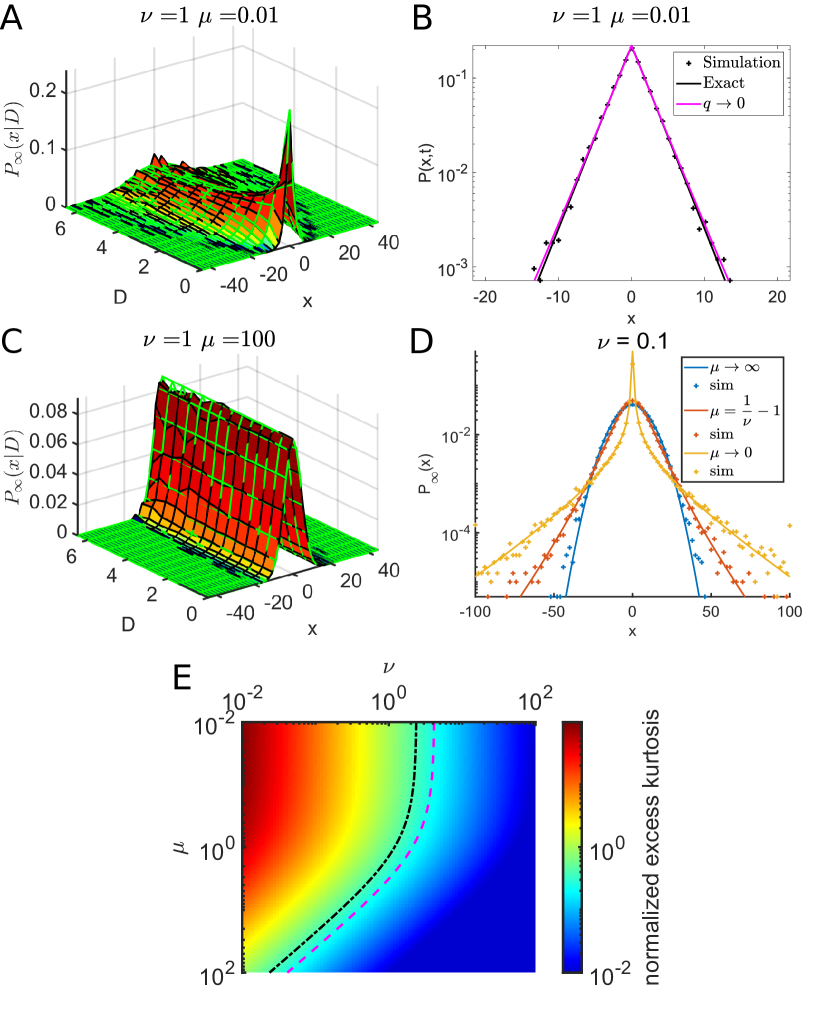
Figure 1: (A) Stationary conditional PDF $P_{\infty}(x|D)$ in the case of temperature fluctuations with parameters $\mu=0.1$, $\nu=1$, $\tau_{x}=20$ and $\bar{D}=1$. (B) Stationary PDF in the case $\mu=0.01$ based on simulation (black dots), overlayed with the exact expression (black curve) and with the small frequency behavior ($q\to 0$) corresponding to the limit $\mu\to 0$. (C) Stationary conditional PDF $P_{\infty}(x|D)$ in the case of temperature fluctuations with parameters $\mu=10$, $\nu=1$, $\tau_{x}=20$ and $\bar{D}=1$. (D) Simulated (dots) and theoretical (lines) stationary PDF as a function of the ratio of correlation times taking values $\mu=0.01$ (yellow), $\mu=1/\nu-1=1$ (red), $mu=100$ (blue) with parameters $\nu=0.1$,$\tau_{x}=20$ and $\bar{D}=1$. (E) Normalized excess kurtosis of the long-time stationary PDF as a function of $\mu$ and $\nu$. Black dashed line corresponds to the value for which transition from Laplace to Gaussian is detected using kundu04 and purple dashed line corresponding to the value for which Jarque-Bera test Jarque1980 detects Gaussian PDF.

II.4 Ergodicity

When temperature fluctuates, the system is generally out of equilibrium. However, in our case, temperature fluctuates around an average with a stationary distribution at long-time. Therefore, one can wonder whether this model shows ergodicity breaking or not. In the case of infinitely divisible processes one can use the Wiener-Khintchine theorem to prove ergodicity if the autocorrelation function vanishes Khinchin1949 ; Lapas2008 ; Burov2010 . Other approaches make use of the dynamical functional Magdziarz2011 ; Janczura2015 ; Lanoiselee2016 . But in our case the process is not infinitely divisible so these tools are not suitable. We then question ergodicity in a weaker sense by determining the time-averaged mean square displacement and comparing it to the generalized MSD following the strategy developed in Mardoukhi2020 for the case of an OU process with constant diffusion coefficient. For this we first compute the generalized MSD $\langle(x_{t+\Delta}-x_{t})^{2}\rangle$. Next, we compute the average over $x_{0}$ for which the process is assumed to start at equilibrium yielding $\langle x_{0}\rangle=\bar{x}$, $\langle x_{0}^{2}\rangle=\bar{D}\tau_{x}$ and $\langle D_{0}\rangle=\bar{D}$. Thus, we have

$$\langle(x_{t+\Delta}-x_{t})^{2}\rangle=2\bar{D}\tau_{x}\left(1-e^{-\Delta/\tau_{x}}\right)\,.$$ (33)

The ensemble averaged TAMSD follows

$$\langle\delta^{2}(\Delta,t)\rangle = 2\bar{D}\tau_{x}\left(1-e^{-\Delta/\tau_{x}}\right).$$ (34)

Finally, we compute the ergodicity breaking parameter He2008 ; Schwarzl2017

$$EB(\Delta)=\lim_{t\to\infty}\frac{\langle\delta^{2}(\Delta,t)\rangle}{\langle(x_{t+\Delta}-x_{t})^{2}\rangle}-1=0$$ (35)

which is equal to $0$, thus proving ergodicity in the weak sense. Despite temperature fluctuations, the second moment is ergodic.

III Diffusive model in harmonic potential – The case of fluctuating friction coefficient

In this section we study the case of a particle diffusing in a harmonic potential, where friction $\gamma_{t}$ fluctuates over time while temperature remains constant. To apply the same model for diffusivity as in Sec. II, we use the relationship described in Eq. (1) to express the time-dependent friction coefficient $\gamma_{t}$ as a function of $D_{t}$ in the form

$$\gamma_{t}=\frac{k_{B}T}{D_{t}}\,.$$ (36)

In this case, the coupled Langevin equation for position $x_{t}$ and diffusivity $D_{t}$ is written as

$$\left\{\begin{array}[]{ll}dx_{t}=-\frac{1}{\tau_{x}}\frac{D_{t}}{\bar{D}}(x_{t}-\bar{x})dt+\sqrt{2D_{t}}\,dW_{t}^{(1)}\\ dD_{t}=-\frac{1}{\tau_{D}}(D_{t}-\bar{D})dt+\sigma\sqrt{2D_{t}}\,dW_{t}^{(2)}\end{array}\,,\right.$$ (37)

where the inverse positional correlation time $\frac{1}{\tau_{x}}\frac{D_{t}}{\bar{D}}$ is obtained by combining Eq.(8) and Eq.(9). It is clear that, contrarily to Sec. II, the inverse correlation time fluctuates around its mean $1/\tau_{x}$ in the same way as diffusivity does fluctuate around $\bar{D}$. Note that the equation for diffusivity is identical to Eq.(7).

To study this equation, we rescale time by diffusivity $dt^{*}=D_{t}dt$, where $t^{*}$ has a unit of integrated diffusivity ($m^{2}$). This variable change allows one to treat the process within the subordination framework Chechkin2017 . The rescaled equation gives

$$\left\{\begin{array}[]{ll}dx_{t^{*}}=-\frac{1}{\bar{D}\tau_{x}}(x_{t^{*}}-\bar{x})dt^{*}+\sqrt{2}\,dW_{t^{*}}^{(1)}\\ dt^{*}=D_{t}dt,\\ dD_{t}=-\frac{1}{\tau_{D}}(D_{t}-\bar{D})dt+\sigma\sqrt{2D_{t}}\,dW_{t}^{(2)}\end{array}\,,\right.$$ (38)

where the first equation corresponds to the parent process that is an OU process and the second equation corresponds to the subordinator that defines the integrated diffusivity $t^{*}=\int_{0}^{t}D_{s}ds$.

The probability density function of the parent process $p(x,t^{*})$ for the position $x$ as a function of the subordinator $t^{*}$ is Gaussian with mean $\langle x_{t^{*}}\rangle=\bar{x}+(x_{0}-\bar{x})e^{-t^{*}/(\bar{D}\tau_{x})}$ and variance $\langle(x_{t^{*}}-\langle x_{t^{*}}\rangle)^{2}\rangle=\bar{D}\tau_{x}\left(1-e^{-2t^{*}/(\bar{D}\tau_{x})}\right)$. The corresponding characteristic function of the parent process takes the form

$$\tilde{p}(q,t^{*}) = e^{-iq\left[\bar{x}+(\bar{x}-x_{0})e^{-t^{*}/(\bar{D}\tau_{x})}\right]}$$ (39)

$$\times e^{-\frac{q^{2}}{2}\bar{D}\tau_{x}(1-e^{-2t^{*}/(\bar{D}\tau_{x})})}\,.$$

To obtain the characteristic function of the process, one needs to integrate the characteristic function $\tilde{p}(q,t^{*})$ of the parent process over the probability density $\Pi(t^{*},t)$ of integrated diffusivity, namely

$$\tilde{P}(q,t)=\int_{0}^{\infty}\tilde{p}(q,t^{*})\Pi(t^{*},t)dt^{*}.$$ (40)

Unfortunately, the exact expression for $\Pi(t^{*},t)$ is unknown, as the integral cannot be computed explicitly. However, the integral representation of the characteristic function in Eq.(40) will be useful to find the moments of the process in the next section.

III.1 Moments and normalized excess kurtosis

Now we study the effect of friction fluctuations on the moments and the normalized excess kurtosis of the process. At small values $q$ the characteristic function reads

$$\tilde{P}(q,t)\sim 1-iq\int_{0}^{\infty}\left[\bar{x}+(\bar{x}-x_{0})e^{-\frac{t^{*}}{(\bar{D}\tau_{x})}}\right]\Pi(t^{*},t)dt^{*}$$

$$-q^{2}\frac{\bar{D}\tau_{x}}{2}\int_{0}^{\infty}\left(1-e^{-2t^{*}/(\bar{D}\tau_{x})}\right)\Pi(t^{*},t)dt^{*}$$ (41)

$$+\frac{q^{4}}{2}\left(\frac{\bar{D}\tau_{x}}{2}\right)^{2}\int_{0}^{\infty}\left(1-e^{-2t^{*}/(\bar{D}\tau_{x})}\right)^{2}\Pi(t^{*},t)dt^{*}\,.$$

Using the formula for the moments $\langle x^{k}(t)\rangle=i^{-k}\frac{d^{k}\tilde{P}(q,t)}{dq^{k}}|_{q=0}$, we deduce the first moment

$$\langle x_{t}\rangle=\bar{x}+(\bar{x}-x_{0})\hat{\Pi}(s,t)\Bigg{|}_{s=1/(\bar{D}\tau_{x})},$$ (42)

where $\hat{\Pi}(s,t)$ stand for the Laplace transform of the integrated diffusivity PDF. Similarly, one can find the second moment, i. e.

$$\langle x_{t}^{2}\rangle=\bar{D}\tau_{x}\left(1-\hat{\Pi}(s,t)\Big{|}_{s=2/(\bar{D}\tau_{x})}\right).$$ (43)

Both first and second moments are strongly affected by friction fluctuations (as opposed to the temperature fluctuation case) because the positional correlation time is fluctuating.

For our model, it is known Dufresne1990 ; Lanoiselee2018a that

$$\hat{\Pi}(s,t|D_{0}) = \left[\frac{e^{\frac{t}{2\tau_{D}}}}{\cosh(\frac{\omega_{s}t}{2\tau_{D}})+\frac{1}{\omega_{s}}\sinh(\frac{\omega_{s}t}{2\tau_{D}})}\right]^{\nu}$$

$$\times\exp\left[-\frac{sD_{0}\tau_{D}}{\omega_{s}}\frac{2\sinh(\frac{\omega_{s}t}{2\tau_{D}})}{\cosh(\frac{\omega_{s}t}{2\tau_{D}})+\frac{1}{\omega_{s}}\sinh(\frac{\omega_{s}t}{2\tau_{D}})}\right],$$

with $\omega_{s}=\sqrt{1+4s\sigma^{2}\tau_{D}^{2}}$. Averaging over $D_{0}$, this expression yields

$$\hat{\Pi}(s,t) = \left(\frac{2e^{-\alpha_{s}t}}{1+e^{-\frac{\omega_{s}t}{\tau_{D}}}}\right)^{\nu}$$ (45)

$$\times \frac{1}{\left(1+\frac{1}{\omega_{s}}\left(1+s\frac{2\bar{D}\tau_{D}}{\nu}\right)\tanh\left(\frac{\omega_{s}t}{2\tau_{D}}\right)\right)^{\nu}}$$

with $\alpha_{s}=(\omega_{s}-1)/(2\tau_{D})$, and $\displaystyle\lim_{x\to\infty}\tanh(x)=1$. Here, friction fluctuations strongly affect the relaxation time to positional equilibrium. For an arbitrary number $p$, we have $\omega_{2p/(\bar{D}\tau_{x})}=\sqrt{1+4p/(\mu\nu)}$ which explicitly depends on the product $\nu\mu$. In the case where $\mu$ is small, we have $\alpha_{2p/(\bar{D}\tau_{x}}\approx 2\sqrt{p\nu/(\tau_{D}\tau_{x})}$ such that the relaxation does not only depend on $\tau_{x}$ but also on the product with $\tau_{D}$ thus explaining the much slower relaxation of friction fluctuations compared to temperature fluctuations as illustrated in Fig.(2.A) using the same parameters for both cases.

However, when the lengthscale of thermal fluctuations $\sqrt{\bar{D}\tau_{x}}$ is larger than the lengthscale associated with diffusivity fluctuations $\sigma\tau_{D}$, then diffusive molecules have enough time to average out diffusivity fluctuations. Thus, the expression of the MSD turns to that of temperature fluctuation case Eq.(29), but the PDF is Gaussian so the dynamic is that of a simple OU process.

In any case, at long times the MSD reads

$$\langle x^{2}(t\to\infty)\rangle=\bar{D}\tau_{x}\,.$$ (46)

Similarly the fourth moment is equal to

$$\langle x_{t}^{4}\rangle = 3\left(\bar{D}\tau_{x}\right)^{2}\Big{(}1-2\hat{\Pi}(s,t)\Big{|}_{s=2/(\bar{D}\tau_{x})}$$ (47)

$$+ \hat{\Pi}(s,t)\Big{|}_{s=4/(\bar{D}\tau_{x})}\Big{)}\,.$$

From which we deduce the normalized excess kurtosis, namely

$$\kappa(t)=\frac{\hat{\Pi}(s,t)\Big{|}_{s=4/(\bar{D}\tau_{x})}-\left(\hat{\Pi}(s,t)\Big{|}_{s=2/(\bar{D}\tau_{x})}\right)^{2}}{\left(1-\hat{\Pi}(s,t)\Big{|}_{s=2/(\bar{D}\tau_{x})}\right)^{2}}\,,$$ (48)

which vanishes in the long-time limit

$$\kappa(t\to\infty)=0\,.$$ (49)

Figure (2.B) shows the decay of the normalized excess kurtosis in the case $\mu\ll 1$ while that of temperature fluctuation remains constant. Moreover, the $2n$-th moment can be computed

$$\langle x^{2n}(t)\rangle = (2n-1)!!\left(\bar{D}\tau_{x}\right)^{n}\Big{(}1$$ (50)

$$+ \sum_{p=1}^{n}(-1)^{p}{n\choose p}\hat{\Pi}(s,t)\Big{|}_{s=2p/(\bar{D}\tau_{x})}\Big{)}\,,$$

where $n!!=n\times(n-2)\times(n-4)\ldots$ is the double factorial. Given that $\displaystyle\lim_{t\to\infty}\hat{\Pi}(s,t)=0$, all the even moments converge to those of a Gaussian distribution in the long-time limit, meaning that the stationary PDF for the position is Gaussian in all scenarios a shown in Fig.(2.C) in striking contrast with temperature fluctuation case. Additionally the conditional probability distribution is independent of $D$ and depends solely on $\bar{D}$ as illustrated in Fig.(2.D).

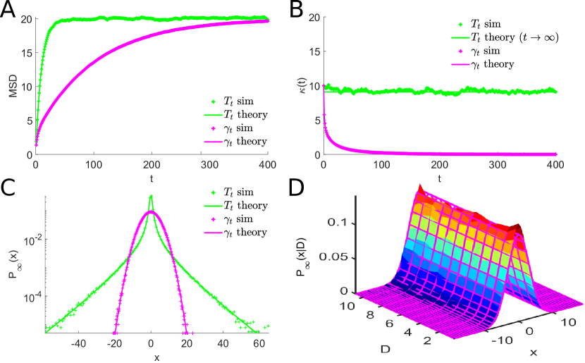
Figure 2: All the results presented in this figure have been obtained with parameters $\bar{D}=1$, $\nu=0.1$, $\tau_{x}=20$ and $\mu=0.1$. (A) Simulation (dots) overlayed with theory (lines) for the MSD in the case of temperature fluctuations (green) and friction fluctuations (magenta). (B) Simulation overlayed with theoretical curve for the normalised excess kurtosis $\kappa(t)$ in the case of temperature fluctuations (green) and friction fluctuations (magenta). Parameters are $\nu=1$, $\mu=0.01$, $tau_{x}=20$ and $\bar{D}=1$. (C) Simulation overlayed with theoretical curve for the the stationary PDF in the case of temperature fluctuations (green) and friction fluctuations (magenta). (D) Simulation (colored surface) overlayed with theory (magenta mesh) for the stationary conditional probability $P_{\infty}(x|D)$ in the case of friction fluctuations.

III.2 Ergodicity

To investigate the ergodic properties, we start with the generalized second moment of the subordinator

$$\left\langle\left(x_{t^{*}+\Delta^{*}}-x_{t^{*}}\right)^{2}\right\rangle=2\bar{D}\tau_{x}\left(1-e^{-\Delta^{*}/(\bar{D}\tau_{x})}\right)\,.$$ (51)

For the parent process the time averaged MSD is equal to the MSD

$$\delta(\Delta^{*},t^{*}) = \left\langle\left(x_{t+\Delta}-x_{t}\right)^{2}\right\rangle$$ (52)

$$= 2\bar{D}\tau_{x}\left(1-e^{-\Delta^{*}/(\bar{D}\tau_{x})}\right)\,.$$

Then we average over the integrated diffusivity probability density for $t^{*}$ at time $t$ and for $\Delta^{*}$ at time $\Delta$ to get

$$\delta^{2}(\Delta,t)=2\bar{D}\tau_{x}\left(1-\hat{\Pi}(s,\Delta)\Bigg{|}_{2/(\bar{D}\tau_{x})}\right).$$ (53)

As a result, the ergodicity breaking parameter is zero. We conclude that for friction fluctuations as well, the process is ergodic in the weak sense.

IV Conclusion

In this article, we have investigated the motion of a particle trapped inside a harmonic potential with diffusing diffusivity. Two cases were considered. The first where diffusing diffusivity is interpreted as temperature fluctuations. In the second case, it was interpreted as friction fluctuations. We showed that, in both cases, two essential quantities are useful to describe the system. The first value is $\nu$, which defines the inverse strength of diffusivity fluctuations, whereas the second is $\mu$, which quantifies the ratio between the position and the diffusivity correlation times. In both cases, when $\nu\to\infty$, diffusivity becomes a constant process, and the usual OU process is recovered at all times. When $\mu\gg 1$, but $\nu$ remains finite, in both cases the initial PDF of displacement shows exponential tails with a shape determined by $\nu$. The models converge to OU because diffusivity has time to self-average before particles can reach positional equilibrium.
However, in all the intermediate cases (finite $\nu$ and $\mu$), their behavior is drastically different. In the case of temperature fluctuations, the stationary long-time PDF displays exponential tails, and in the limit case $\mu\to 0$ the PDF conserves the same shape as in the initial condition. However, the first and second moments are the same as for the OU case, while the fourth moment differs. In turn, for friction fluctuations the long-time stationary PDF is Gaussian in any case while the moments departs from that of an OU process because of the fluctuating positional correlation time.
The main results of the paper are:

• non-Gaussian PDF with continuous model and its ergodic properties;

• generalized Laplace distribution with a confining potential for temperature fluctuations;

• in both studied cases the diffusion coefficient has exactly the same distribution, however we show that depending on whether it is a friction or a temperature fluctuation, the statistical properties of the process are very different.

We anticipate that these new results will be instrumental in understanding what happens to trapped molecules in an experimental setup, and offer far more greater detail than previous methods. Indeed one could test the presence of either temperature of friction fluctuations and use the statistical properties described here to quantify these distinct types of fluctuations. On the theoretical side, our results raise questions about the relationship between the temperature fluctuation case studied here and stochastic resetting that can yield similar stationary PDF with exponential tails.

.

APPENDICES

Appendix A Laplace distribution

The emergence of Laplace (or double exponential statistics) like the Gaussian, for various random observables in nature, engineering, and finance, is widespread. Many examples range from the first law of errors Laplace1986 to Laplace motion Kotz2001 . The Laplace distribution suggests a much better model to describe observations than the Gaussian distribution with common variance, because each observer-instrument has its own variability, and all the participants of observations together result in large errors. Moreover, the explanation of anomalous diffusion tending to the confinement with the Laplace distribution is that diffusive motion, also accompanied by multiple trapping events with infinite mean sojourn time, makes impossible to leave such traps Stanislavsky2021a . The Laplace distribution is also occurred as a steady state of Brownian motion under Poissonian resetting ems20 .

It was shown recently Stanislavsky2021a that the Laplace confinement is present in confined random motions of both G proteins and receptors in living cells. It should be pointed out that the confined distribution form depends on the PDF of the parent process used for subordination. If we take Brownian motion, then the confined distribution has the Laplace form. This means that the presented mechanism can manifest itself as a source of the origin of jumps in heterogeneous systems. It is interesting that Lévy motion as a parent process produces another confinement having the Linnik distribution.

Appendix B Full derivation for the fluctuating temperature case

The corresponding forward Fokker-Planck equation for the joint probability $P(x,D,t|x_{0},D_{0})$ of being at position $x$ and diffusivity $D$ at time $t$ starting from values $x_{0},D_{0}$ is

$$\frac{\partial P(x,D,t|x_{0},D_{0})}{\partial t} = \frac{1}{\tau_{x}}\frac{\partial}{\partial x}\left[(x-\bar{x})P\right]$$ (54)

$$+ D\frac{\partial^{2}}{\partial x^{2}}P+\frac{1}{\tau_{D}}\frac{\partial}{\partial D}\left[(D-\bar{D})P\right]$$

$$+ \sigma^{2}\frac{\partial^{2}}{\partial D^{2}}\left(DP\right)$$

with the initial condition being $P(x,D,0|D_{0})=\delta(x-x_{0})\delta(D-D_{0})$ that is equivalent to

$$\frac{\partial P(x,D,t|x_{0},D_{0})}{\partial t} = \frac{1}{\tau_{x}}\frac{\partial}{\partial x}\left[(x-\bar{x})P\right]$$ (55)

$$+ D\frac{\partial^{2}}{\partial x^{2}}P-\frac{\partial}{\partial D}J_{D}\,,$$

where $J_{D}(D,t)$ is the diffusivity flux, i. e. $J_{D}(D,t)=-\frac{1}{\tau_{D}}\left[(D-\bar{D})P\right]-\sigma^{2}\frac{\partial}{\partial D}\left(DP\right)$. The PDF can be translated in the Fourier (space)-Laplace (diffusivity) domain through the integral transform

$$P^{*}(q,s,t|x_{0},D_{0}) = \int\displaylimits\displaylimits_{-\infty}^{\infty}dx\int\displaylimits\displaylimits_{0}^{\infty}dD\,e^{-sD-iqx}$$ (56)

$$\times P(x,D,t|x_{0},D_{0})\$$

from which we deduce the new equation:

$$\frac{\partial}{\partial t}P^{*}+Q(s)\frac{\partial}{\partial s}P^{*}+\frac{1}{\tau_{x}}q\frac{\partial}{\partial q}P^{*}$$ (57)

$$=\left(-i\frac{1}{\tau_{x}}\bar{x}q-\frac{1}{\tau_{D}}\bar{D}s\right)P^{*}+J_{D}(D=0,t)\,,$$

where $Q(s)=\left(\sigma^{2}s^{2}+\frac{1}{\tau_{D}}s-q^{2}\right)$ and $J_{D}(D=0,t)=(\bar{D}/\tau-\sigma^{2})P(q,D=0|x_{0},D_{0})$.

To ensure diffusivity reaches a stationary distribution, we focus on the case, when there is a reflecting boundary condition at $D=0$. Therefore, the flux cancels at $D=0$ from which $J_{D}(D=0,t)=0$, and we then obtain

$$\frac{\partial}{\partial t}P^{*} + Q(s)\frac{\partial}{\partial s}P^{*}+\frac{1}{\tau_{x}}q\frac{\partial}{\partial q}P^{*}$$ (58)

$$= \left(-i\frac{1}{\tau_{x}}\bar{x}q-\frac{1}{\tau_{D}}\bar{D}s\right)P^{*}$$

with the initial condition taking the form $P^{*}(q,s,0|x_{0},D_{0})=e^{-iqx_{0}}e^{-sD_{0}}$.

B.0.1 Method of characteristics

Our equation (58) is a first order partial differential equation. To solve it, we use the conventional method of characteristics. The Lagrange-Charpit equations Delgado1997 corresponding to the problem are

$$dt = \frac{dq}{\frac{1}{\tau_{x}}q}=\frac{ds}{\left(\sigma^{2}s^{2}+\frac{1}{\tau_{D}}s-q^{2}\right)}$$ (59)

$$= \frac{dP^{*}}{\left(-i\frac{1}{\tau_{x}}\bar{x}q-\frac{1}{\tau_{D}}\bar{D}s\right)}$$

from which we obtain a system of differential equations

$$\left\{\begin{array}[]{ll}\frac{dq}{dt}=\frac{1}{\tau_{x}}q\,,\\ \\ \frac{ds}{dt}=\sigma^{2}s^{2}+\frac{1}{\tau_{D}}s-q^{2}\,,\\ \\ \frac{dP^{*}}{dt}=\left(-i\frac{1}{\tau_{x}}\bar{x}q-\frac{1}{\tau_{D}}\bar{D}s\right)P^{*}\,.\end{array}\right.$$ (60)

The first equation of the system (60) yields

$$q=C_{1}e^{\frac{t}{\tau_{x}}}$$ (61)

with $C_{1}$ an integration constant.

We then substitute it into the second equation to get

$$\frac{ds}{dt}-\sigma^{2}s^{2}-\frac{1}{\tau_{D}}s+C_{1}^{2}e^{2t/\tau_{x}}=0\,.$$ (62)

After the variable change $s=-\frac{1}{\sigma^{2}}y^{\prime}/y$ and the coordinate change $v=\exp(2t/\tau_{x})$ we come to the equation

$$v\frac{d^{2}y}{dv^{2}}+\left(1-\frac{\tau_{x}}{2\tau_{D}}\right)\frac{dy}{dv}-\frac{\sigma^{2}C_{1}^{2}\tau_{x}^{2}}{4}y=0\,.$$ (63)

B.0.2 Solving the second equation

Our equation is of the following form

$$vy^{\prime\prime}+(1-a)y^{\prime}-by=0\,,$$ (64)

for which the solution is expressed in terms of modified Bessel functions abr64 , namely

$$y(v) = c_{1}b^{a/2}v^{a/2}\Gamma(1-a)I_{-a}(2\sqrt{bv})$$

$$+ (-1)^{a}c_{2}b^{a/2}v^{a/2}\Gamma(a+1)I_{a}(2\sqrt{bv})\,.$$

with two integration constants, $c_{1}$ and $c_{2}$. Translating the solution back to our parameters and defining $C_{2}=c_{1}/c_{2}$, as well as $A=c_{2}(-1)^{\frac{\tau_{x}}{2\tau_{D}}}\Gamma(\frac{\tau_{x}}{2\tau_{D}}+1)$, we get

$$y(t) = A\left(\frac{\sigma^{2}C_{1}^{2}\tau_{x}^{2}}{4}\right)^{\frac{\tau_{x}}{4\tau_{D}}}e^{t/(2\tau_{D})}$$ (66)

$$\times\Bigg{(}C_{2}\frac{\Gamma(1-\frac{\tau_{x}}{2\tau_{D}})}{A}I_{-\frac{\tau_{x}}{2\tau_{D}}}(\sigma\tau_{x}|C_{1}|e^{t/\tau_{x}})$$

$$\qquad+I_{\frac{\tau_{x}}{2\tau_{D}}}(\sigma\tau_{x}|C_{1}|e^{t/\tau_{x}})\Bigg{)}\,.$$

From this we can deduce $s$, i. e.

$$s = -\frac{1}{\sigma}|C_{1}|e^{t/\tau_{x}}\Big{(}C_{2}\frac{\Gamma(1-\frac{\tau_{x}}{2\tau_{D}})}{A}I_{1-\frac{\tau_{x}}{2\tau_{D}}}(\sigma\tau_{x}|C_{1}|e^{t\tau_{x}})$$ (67)

$$+ I_{-1+\frac{\tau_{x}}{2\tau_{D}}}(\sigma\tau_{x}|C_{1}|e^{t\tau_{x}})\Big{)}$$

$$\times \Big{(}C_{2}\frac{\Gamma(1-\frac{\tau_{x}}{2\tau_{D}})}{A}I_{-\frac{\tau_{x}}{2\tau_{D}}}(\sigma\tau_{x}|C_{1}|e^{t\tau_{x}})$$

$$+ I_{\frac{\tau_{x}}{2\tau_{D}}}(\sigma\tau_{x}|C_{1}|e^{t\tau_{x}})\Big{)}^{-1}\,.$$

So we obtain

$$C_{2}=-\frac{A}{\Gamma(1-\frac{\tau_{x}}{2\tau_{D}})}W\,,$$ (68)

where

$$W=\left(\frac{I_{-1+\frac{\tau_{x}}{2\tau_{D}}}(\sigma\tau_{x}|q|)+\frac{s\sigma}{|q|}I_{\frac{\tau_{x}}{2\tau_{D}}}(\sigma\tau_{x}|q|)}{\frac{s\sigma}{|q|}I_{-\frac{\tau_{x}}{2\tau_{D}}}(\sigma\tau_{x}|q|)+I_{1-\frac{\tau_{x}}{2\tau_{D}}}(\sigma\tau_{x}|q|)}\right)\,.$$ (69)

B.0.3 Third equation

Then the last equation in Eq.(60) is written as

$$\int\displaylimits\frac{dP}{P}=-i\frac{1}{\tau_{x}}\bar{x}\int\displaylimits q(t)dt-\frac{\bar{D}}{\tau_{D}}\int\displaylimits s(t)dt\,,$$ (70)

for which the solution reads

$$P=C_{4}\exp\left(-i\frac{1}{\tau_{x}}\bar{x}\int\displaylimits q(t)dt-\frac{\bar{D}}{\tau_{D}}\int\displaylimits s(t)dt\right)\,,$$ (71)

where $q$ is substituted from Eq.(61). By definition we have $\int\displaylimits s(t)dt=-\frac{1}{\sigma^{2}}\ln(y(t))$ from which we get

$$P=H(C_{1},C_{2})\exp\left(-i\bar{x}C_{1}e^{\frac{t}{\tau_{x}}}\right)y^{\frac{\bar{D}}{\sigma^{2}\tau_{D}}}\,,$$ (72)

where $H(C_{1},C_{2})$ depends on the constants $C_{1}$ and $C_{2}$.

B.0.4 Initial condition

At $t=0$, we have $P(q,s,t=0)=e^{-iqx_{0}-sD_{0}}$ so that

$$H(C_{1},C_{2}) = \exp\left(-iC_{1}x_{0}\right)\exp\left(i\bar{x}C_{1}\right)$$

$$\times\exp\left(-D_{0}F(C_{1},C_{2})\right)$$

$$\times\left[G(C_{1},C_{2})\right]^{-\frac{\bar{D}}{\sigma^{2}\tau_{D}}}\,,$$

where $G(C_{1},C_{2})=y(C_{1},C_{2},t=0)$ and $F(C_{1},C_{2})=s(C_{1},C_{2},t=0)$. We then replace $C_{1}(q,t),C_{2}(q,s,t)$ by their expressions in $P$.

B.0.5 Averaging over $D_{0}$

Injecting Eq.(B.0.4) into Eq.(72), we obtain the following propagator

$$P^{*}(q,s,t|x_{0},D_{0}) = \exp\left(-D_{0}F(C_{1},C_{2})\right)$$

$$\times \exp\left(-iC_{1}(x_{0}-\bar{x}(1-e^{\frac{t}{\tau_{x}}}))\right)$$

$$\times \left(\frac{y}{G(C_{1},C_{2})}\right)^{\frac{\bar{D}}{\sigma^{2}\tau_{D}}}\,.$$

Next, we integrate over the initial distribution of diffusivity $D_{0}$ in the form

$$\Pi(D_{0})=\frac{D_{0}^{\nu-1}}{\Gamma(\nu)\bar{D}^{\nu}}\exp(-D_{0}/\bar{D})$$ (75)

such that the propagator becomes

$$P^{*}(q,s,t|x_{0})=\exp\left(-iq\left(\bar{x}(1-e^{-t/\tau_{x}})+x_{0}e^{-t/\tau_{x}}\right)\right)$$

$$\times\left(\frac{y(C_{1},C_{2})}{G(C_{1},C_{2})\left(1+\bar{D}F(C_{1},C_{2})\right)}\right)^{\frac{\bar{D}}{\sigma^{2}\tau_{D}}}\,.$$ (76)

B.0.6 Averaging over $D$

To find the characteristic function $P^{*}(q,t|x_{0})$, we average over $D$ by simply setting $s=0$. Thus, we deduce

$$W=\left(\frac{I_{-1+\frac{\tau_{x}}{2\tau_{D}}}(\sigma\tau_{x}|q|)}{I_{1-\frac{\tau_{x}}{2\tau_{D}}}(\sigma\tau_{x}|q|)}\right)\,.$$ (77)

In this case we inserted expressions for $y(C_{1},C_{2})$ and $G(C_{1},C_{2})$ to get this expression. Next, we can also include the expression for $F(C_{1},C_{2})$. Using the property $I_{-\nu}(z)=I_{\nu}(z)+(2/\pi)\sin(\nu\pi)K_{\nu}(z)$ and the Wronskian formula $W\{K_{-\mu}(b),I_{-\mu}(b)\}=I_{-\mu}(b)K_{1-\mu}(b)+K_{-\mu}(b)I_{1-\mu}(b)=1/b$, we come to the full characteristic function Eq.(12). One can check normalization by setting $q=0$ and verify that $P^{*}(q=0,t|x_{0})=1$.

Appendix C Large order development of $I_{\beta}(b)$

Based on the asymptotic large order expansion for $I_{\mu-1}(b)$, we start with the integral representation

$$I_{\beta}(b)=\frac{(b/2)^{\beta}}{\sqrt{\pi}\Gamma(\beta+1/2)}\int\displaylimits_{-1}^{1}(1-t^{2})^{\beta-1/2}e^{-bt}dt\,.$$ (78)

With help of the variable change $-u^{2}=\ln(1-t^{2})$ from which $t=\sqrt{1-e^{-u^{2}}}$ and $dt=\frac{ue^{-u^{2}}}{\sqrt{1-e^{-u^{2}}}}du$ we proceed to

$$I_{\beta}(b)=\frac{(b/2)^{\beta}}{\sqrt{\pi}\Gamma(\beta+1/2)}\int\displaylimits_{\mathbb{R}}e^{-\beta u^{2}}f(u)du\,,$$ (79)

where $f(u)=ue^{-b\sqrt{1-e^{-u^{2}}}}\frac{e^{-u^{2}/2}}{\sqrt{1-e^{-u^{2}}}}$. Next, we find the asymptotic behavior for large $\mu$ written as

$$\frac{z^{\beta}}{u^{\beta}\Gamma(\beta+1/2)}=\frac{1}{\sqrt{2\pi}}\left(\frac{eb}{2\beta}\right)^{\beta}+O(\beta^{-1-\beta})\,.$$ (80)

For $f(u)$ we expand $u$ for small order

$$f(u)\approx e^{-bu}(1-u^{2}/2)\,.$$ (81)

The integral over $u$ yields

$$\int\displaylimits_{\mathbb{R}}e^{-\beta u^{2}}f(u)du=e^{b^{2}/(4\beta)}\frac{\sqrt{\pi}}{4\beta^{3/2}}\left(\frac{8\beta^{2}-b^{2}}{2\beta}-1\right)\,.$$ (82)

So we deduce

$$I_{\beta}(b)\approx\frac{e^{b^{2}/(4\beta)}}{\sqrt{2}}\left(\frac{eb}{2\beta}\right)^{\beta}\frac{1}{4\beta^{3/2}}\left(\frac{8\beta^{2}-b^{2}}{2\beta}-1\right)\,.$$ (83)

Appendix D Fourth moment computation

In this section we study the fourth moment in the case of temperature fluctuations. For this purpose we proceed to the variable change $z_{t}=x_{t}^{2}$ for which the integral representation is

$$z_{t} = z_{0}e^{-2t/\tau_{x}}+\int\displaylimits_{0}^{t}2D_{s}e^{2(s-t)/\tau_{x}}ds$$ (84)

$$+\int\displaylimits_{0}^{t}2e^{2(s-t)/\tau_{x}}\sqrt{2z_{s}D_{s}}dW_{s}$$

from which we deduce the integral representation for the fourth moment

$$\langle x_{t}^{4}\rangle = \langle z_{t}^{2}\rangle=\langle x_{0}^{4}\rangle e^{-4t/\tau_{x}}$$ (85)

$$+ 4e^{-4t/\tau_{x}}\int\displaylimits_{0}^{t}\int\displaylimits_{0}^{t}e^{2(s_{1}+s_{2})/\tau_{x}}\langle D_{s_{1}}D_{s_{2}}\rangle ds_{1}ds_{2}$$

$$+ 8\int\displaylimits_{0}^{t}e^{4(s-t)/\tau_{x}}\langle x_{s}^{2}D_{s}\rangle ds\,.$$

We proceed to use the It$\hat{\rm o}$ formula for the variable change from $x$ to $x^{2}$

$$\left\{\begin{array}[]{ll}dx_{t}^{2}=\left(-\frac{2}{\tau_{x}}x_{t}^{2}+2D_{t}\right)dt+2x_{t}\sqrt{2D_{t}}dW_{t}^{(1)}\\ dD_{t}=-\frac{1}{\tau_{D}}(D_{t}-\bar{D})dt+\sigma\sqrt{2D_{t}}dW_{t}^{(2)}\end{array}\,.\right.$$ (86)

From the It$\hat{\rm o}$ product rule we have

$$x_{t}^{2}D_{t} = x_{0}^{2}D_{0}+\int_{0}^{t}x_{s}^{2}dD_{s}$$ (87)

$$+ \int_{0}^{t}D_{s}dx_{s}^{2}+\int_{0}^{t}\langle dx_{s}^{2}dD_{s}\rangle$$

with the last term being equal to zero because of the independence of Wiener processes $W_{t}^{(1)}$ and $W_{t}^{(2)}$. From $\langle x_{t}^{2}D_{t}\rangle$ it follows an integral equation in the form

$$y(t)=y(0)-a\int_{0}^{t}y(s)ds+\int_{0}^{t}b(s)ds\,,$$ (88)

where $a=\frac{2}{\tau_{x}}+\frac{1}{\tau_{D}}$ and $b(t)=\langle x_{s}^{2}\rangle\bar{D}/\tau_{D}+2\langle D_{s}^{2}\rangle$. Taking the derivative on both sides, we get

$$y^{\prime}(t)=-ay(t)+b^{\prime}(t)\,,$$ (89)

from which we have

$$\langle x_{t}^{2}D_{t}\rangle=\int_{0}^{t}e^{(s-t)/\tau_{x}}\left(\langle x_{s}^{2}\rangle\bar{D}/\tau_{D}+2\langle D_{s}^{2}\rangle\right)ds\,.$$ (90)

The exact calculation is achievable, although it is tedious and cumbersome. Instead we find it more informative to focus on the long-time limit. When $t\to\infty$, only constant terms contribute to convolution integrals from which we deduce Eq. (30).

References

- (1) S. Shashkova, and M.C. Leake, Single-molecule fluorescence microscopy review: shedding new light on old problems. Biosci. Rep. 37(4) BSR20170031 (2017).
- (2) M. Lelek, M. T. Gyparaki, G. Beliu, F. Schueder, J. Griffié, S. Manley, R. Jungmann, M. Sauer, M. Lakadamyali, and C. Zimmer, Single-molecule localization microscopy. Nat Rev Meth. Prim. 1, 39 (2021).
- (3) C. Manzo and M.F. Garcia-Parajo, A review of progress in single particle tracking: from methods to biophysical insights, Rep. Prog. Phys. 78 124601 (2015).
- (4) K. Jaqaman, D. Loerke, M. Mettlen, H. Kuwata, S. Grinstein, S.L. Schmid, and Gaudenz Danuser, Robust single-particle tracking in live-cell time-lapse sequences. Nat Methods 5, 695–702 (2008).
- (5) K. I. Mortensen, L. Stirling Churchman, J. A. Spudich, and H. Flyvbjerg, Optimized localization analysis for single-molecule tracking and super-resolution microscopy Nat. Methods 7, 377–381 (2010).
- (6) J.-Y. Tinevez, N. Perry, J. Schindelin, G. M. Hoopes, G. D. Reynolds, E. Laplantine, and K. W. Eliceiri, TrackMate: An open and extensible platform for single-particle tracking. Methods, 115, 80–90 (2017).
- (7) A. Speiser, L.-R. Müller, P. Hoess, U. Matti, C. J. Obara, W. R. Legant, A. Kreshuk, J. H. Macke, J. Ries, and S. C. Turaga, Deep learning enables fast and dense single-molecule localization with high accuracy. Nat. Methods 18, 1082–1090 (2021).
- (8) C. L. Vestergaard, P. C. Blainey, and H. Flyvbjerg, Optimal estimation of diffusion coefficients from single-particle trajectories Phys. Rev. E 89, 022726 (2014).
- (9) N. Hoze and D. Holcman, Recovering a stochastic process from super-resolution noisy ensembles of single-particle trajectories Phys. Rev. E 92, 052109 (2015).
- (10) J. Szwabinski and A. Weron (Eds.), Recent Advances in Single-Particle Tracking: Experiment and Analysis (MDPI, Basel, 2022).
- (11) Y. Lanoiselée, J. Grimes, Z. Koszegi, and D. Calebiro, Detecting transient trapping from a single trajectory: a atructural approach, Entropy 23, 1044 (2021).
- (12) J. Janczura, P. Kowalek, H. Loch-Olszewska, J. Szwabiński, and A. Weron, Classification of particle trajectories in living cells: Machine learning versus statistical testing hypothesis for fractional anomalous diffusion, Phys. Rev. E 102, 032402 (2020).
- (13) G. Muoz-Gil, G. Volpe, M. A. Garcia-March, et al., Objective comparison of methods to decode anomalous diffusion, Nature Communications 12, 6253 (2021).
- (14) H. Verdier, M. Duval, F. Laurent, A. Cassé, C. L. Vestergaard and JB. Masson, Learning physical properties of anomalous random walks using graph neural networks, J. Phys. A 54, 23 (2021).
- (15) K. Burnecki and A. Weron, Algorithms for testing of fractional dynamics: a practical guide to ARFIMA modelling, J. Stat. Mech. P10036 (2014).
- (16) A.V. Weigel, B. Simon, M.M. Tamkun, and D. Krapf, Ergodic and nonergodic processes coexist in the plasma membrane as observed by single-molecule tracking, Proc. Nat. Acad. Sci. 108 (16) 6438-6443 (2011).
- (17) J. Klafter, S. C. Lim, and R. Metzler (Eds.), Fractional Dynamics. Recent Advances (World Scientific Publ. Co., Singapore, 2012).
- (18) N. Hoze, D. Nair, E. Hosy, C. Sieben, S. Manley, A. Herrmann, J.-B. Sibarita, D. Choquet, and David Holcman, Heterogeneity of AMPA receptor trafficking and molecular interactions revealed by superresolution analysis of live cell imaging Proc. Nat. Acad. Sci. 109(42) 17052-17057 (2012).
- (19) T. Sungkaworn, M.-L. Jobin, K. Burnecki, A.Weron, M. Lohse, and D. Calebiro, Single-molecule imaging reveals receptor G protein interactions at cell surface hot spots, Nature (London) 550, 543 (2017).
- (20) A. Weron, J. Janczura, E. Boryczka, T. Sungkaworn, and D. Calebiro, Statistical testing approach for fractional anomalous diffusion classification, Phys. Rev. E 99, 042149 (2019).
- (21) D. Calebiro, Z. Koszegi, Y. Lanoiselée, T. Miljus, and S. O’Brien. G protein-coupled receptor-G protein interactions: a single-molecule perspective. Physiol Rev. 101(3), 857-906 (2021)
- (22) I. Bronstein, Y. Israel, E. Kepten, S. Mai, Y. Shav-Tal, E. Barkai, and Y. Garini, Transient Anomalous Diffusion of Telomeres in the Nucleus of Mammalian Cells, Phys. Rev. Lett. 103, 018102 (2009).
- (23) M. J. Saxton 2007 A biological interpretation of transient anomalous subdiffusion. I. Qualitative model Biophys. J. 92 1178–91 (2007).
- (24) T. Uneyama, T. Miyaguchi, and T. Akimoto, Fluctuation analysis of time-averaged mean-square displacement for the Langevin equation with time-dependent and fluctuating diffusivity,Physical Review E 92(3), 032140 (2015).
- (25) D. S. Grebenkov, Time-averaged mean square displacement for switching diffusion, Phys. Rev. E 99, 032133 (2019).
- (26) B. Wang, S. M. Antony, S. C. Bae, and S. Granick, Anomalous yet Brownian process, Natl. Acad. Sci. USA 106, 15160 (2009).
- (27) B. Wang, J. Kuo, S. C. Bae, and S. Granick, When Brownian diffusion is not Gaussian, Nat. Mater. 11, 481 (2012).
- (28) M. V. Chubynsky and G. W. Slater, Diffusing diffusivity: A model for anomalous, yet Brownian diffusion, Phys. Rev. Lett. 113, 098302 (2014).
- (29) R. Jain and K. L. Sebastian, Diffusion in a crowded rearranging environment, J. Phys. Chem. B 120, 3988 (2016).
- (30) A. V. Chechkin, F. Seno, R. Metzler and I. M. Sokolov, Brownian yet non-Gaussian diffusion: From superstatistics to subordination of diffusing diffusivities, Phys. Rev. X 7, 021002 (2017).
- (31) Y. Lanoiselée and D. S. Grebenkov, A model of non-Gaussian diffusion in heterogeneous media, J. Phys. A: Math. Theor. 51, 145602 (2018).
- (32) C. Beck, Dynamical foundations of nonextensive statistical mechanics, Phys. Rev. Lett. 87, 180601 (2001).
- (33) V. Sposini, A. V. Chechkin, F. Seno, G. Pagnini, and R. Metzler, Random diffusivity from stochastic equations: comparison of two models for Brownian yet non-Gaussian diffusion, New J. Phys. 20, 043044 (2018).
- (34) W. Wang, F. Seno, I. M. Sokolov, A. V. Chechkin, and R. Metzler, Unexpected crossovers in correlated random-diffusivity processes, New J. Phys. 22, 083041 (2020).
- (35) T. Miyaguchi, T. Akimoto, and E. Yamamoto, Langevin equation with fluctuating diffusivity: A two-state model, Phys. Rev. E 94(1), 012109 (2016).
- (36) T. Miyaguchi, T. Uneyama, and T. Akimoto, Brownian motion with alternately fluctuating diffusivity: stretched-exponential and power-law relaxation, Phys. Rev. E 100(1), 012116 (2019).
- (37) Y. Lanoiselée and D. S Grebenkov, Non-Gaussian diffusion of mixed origins, J. Phys. A: Math. Theor. 52, 304001 (2019).
- (38) E. Barkai and S. Burov, Packets of diffusing particles exhibit universal exponential tails, Phys. Rev. Lett. 124, 060603 (2020).
- (39) L. Luo, and M. Yi, Non-Gaussian diffusion in static disordered media, Phys. Rev. E 97, 042122 (2018).
- (40) E. B. Postnikov, A. V. Chechkin and I. M. Sokolov, Brownian yet non-Gaussian diffusion in heterogeneous media: from superstatistics to homogenization, New J. Phys. 22, 063046 (2020).
- (41) M. Cebecauer, M. Amaro, P. Jurkiewicz, M.J. Sarmento, R. Šachl, L. Cwiklik, and M. Hof, Membrane Lipid Nanodomains Chem. Rev., 118 (23), 11259–11297 (2018).
- (42) E. Cocucci, F. Aguet, S. Boulant, and T. Kirchhausen, The First Five Seconds in the Life of a Clathrin-Coated Pit, Cell 150 (3), 495-507 (2012).
- (43) A. Kusumi, C. Nakada, K. Ritchie, K. Murase, K. Suzuki, H. Murakoshi, R.S. Kasai, J. Kondo, and T. Fujiwara, Paradigm Shift of the Plasma Membrane Concept from the Two-Dimensional Continuum Fluid to the Partitioned Fluid: High-Speed Single-Molecule Tracking of Membrane Molecules, Ann. Rev. Biophys. Biomol. Struct. 34, 351-378 (2005).
- (44) A. Taflia and D. Holcman, Dwell time of a Brownian molecule in a microdomain with traps and a small hole on the boundary, J. Chem. Phys. 126 (23), 234107 (2007).
- (45) Y. Lanoiselée, N. Moutal and D.S. Grebenkov, Diffusion-limited reactions in dynamic heterogeneous media. Nat. Commun. 23;9(1):4398 (2018).
- (46) V. Sposini, A. Chechkin and R. Metzler, First passage statistics for diffusing diffusivity, J. Phys. A 52, 4 (2018).
- (47) D. S. Grebenkov, V. Sposini, R. Metzler, G. Oshanin and F. Seno, Exact first-passage time distributions for three random diffusivity models, J. Phys. A 54.4 (2021).
- (48) E. Yamamoto, T. Akimoto, A. Mitsutake, and R. Metzler, Universal Relation between Instantaneous Diffusivity and Radius of Gyration of Proteins in Aqueous Solution. Phys. Rev. Lett. 126, 128101 (2021).
- (49) K. Okabe, R. Sakaguchi, B. Shi, et al., Intracellular thermometry with fluorescent sensors for thermal biology, Pflugers Arch - Eur. J. Physiol. 470, 717 (2018).
- (50) K. Oyama, M. Gotoh, Y. Hosaka, T. G. Oyama, A. Kubonoya, Y. Suzuki, T. Arai, S. Tsukamoto, Y. Kawamura, H. Itoh, S. A. Shintani, T. Yamazawa, M. Taguchi, Sh. Ishiwata, N. Fukuda, Single-cell temperature mapping with fluorescent thermometer nanosheets. J. Gen. Physiol. 152(8), e201912469 (2020).
- (51) R. S. Balaban, How hot are single cells? J. Gen. Physiol. 152(8), e202012629 (2020).
- (52) M.R. Evans, S.N. Majumdar, and G. Schehr, Stochastic resetting and applications, J. Phys. A: Math. Theor. 53, 193001 (2020).
- (53) A. Stanislavsky and A. Weron, Subdiffusive search with home returns via stochastic resetting: A subordination scheme approach, J.Phys. A: Math. Theor. 55(7), 074004 (2022).
- (54) A. Stanislavsky and A. Weron, Optimal non-Gaussian search with stochastic resetting, Phys. Rev. E 104, 014125 (2021).
- (55) T. Uneyama, T. Miyaguchi, and T. Akimoto, Relaxation functions of the Ornstein-Uhlenbeck process with fluctuating diffusivity, Phys. Rev. E 99, 032127 (2019).
- (56) N. Tyagi, and B.J. Cherayil, J. Phys. Chem. B, 121 (29), 7204-7209 (2017).
- (57) R. Jain, and K.L. Sebastian , J. Chem. Sci. 126, 929-937 (2017).
- (58) J. Gajda and A. Wyłomańska, Time-changed Ornstein–Uhlenbeck process, J. Phys. A: Math. Theor. 48, 135004 (2015).
- (59) M. Abramowitz and I. A. Stegun, Handbook of Mathematical Functions with Formulas, Graphs, and Mathematical Tables (Dover, New York, 1964).
- (60) D. Madan and E. Seneta, The variance gamma (V.G.) model for share market returns, Journal of Business 63, 511 (1990).
- (61) D. Madan, P. Carr, and E. Chang, The variance gamma process and option pricing. European Finance Review 2, 79 (1998).
- (62) D. Kundu, In: N. Balakrishnan, H. N. Nagaraja, and N. Kannan (Eds.) Advances in Ranking and Selection, Multiple Comparisons, and Reliability, Statistics for Industry and Technology, (Birkhäuser, Boston, 2005), pp. 65-79.
- (63) C. M. Jarque and A. K. Bera, Efficient tests for normality, homoscedasticity and serial independence of regression residuals, Economics Lett. 6(3), 255 (1980).
- (64) A. I. Khinchin, Mathematical Foundations of Statistical Mechanics (Dover, New York, 1949).
- (65) L. C. Lapas, R. Morgado, M. H. Vainstein, J. M. Rubi, and F. A. Oliveira, Khinchin theorem and anomalous diffusion, Phys. Rev. Lett. 101, 230602 (2008).
- (66) S. Burov, R. Metzler, and E. Barkai, Aging and nonergodicity beyond the Khinchin theorem, Proc. Natl. Acad. Sci. USA 107, 13228 (2010).
- (67) M. Magdziarz and A. Weron, Anomalous diffusion: Testing ergodicity breaking in experimental data, Phys. Rev. E 84, 051138 (2011).
- (68) J. Janczura and A. Weron, Ergodicity testing for anomalous diffusion: Small sample statistics, J. Chem. Phys. 142, 144103 (2015).
- (69) Y. Lanoiselée and D. S. Grebenkov, Revealing nonergodic dynamics in living cells from a single particle trajectory, Phys. Rev. E 93, 052146 (2016).
- (70) Y. Mardoukhi, A. Chechkin, and R. Metzler, Spurious ergodicity breaking in normal and fractional Ornstein–Uhlenbeck process, New J. Phys. 22, 073012 (2020).
- (71) Y. He, S. Burov, R. Metzler, and E. Barkai, Random time-scale invariant diffusion and transport coefficients, Phys. Rev. Lett. 101, 058101 (2008).
- (72) M. Schwarzl, A. Godec, and R. Metzler, Quantifying non-ergodicity of anomalous diffusion with higher order moments, Sci. Rep. 7, 3878 (2017).
- (73) D. Dufresne, Working Paper, University of Melbourne, 2001.
- (74) P. S. Laplace, Memoir on the probability of the causes of events, Statistical Science 1 364–78 (1986).
- (75) S. Kotz, T. Kozubowski, and K. Podgorski, The Laplace Distribution and Generalizations: A Revisit with Applications to Communications, Economics, Engineering, and Finance (Boston: Birkhauser) (2001).
- (76) A. Stanislavsky and A. Weron, Confined with Laplace and Linnik statistics, J. Phys. A: Math. Theor. 54 (2021).
- (77) M. Delgado, Classroom Note: The Lagrange-Charpit Method, SIAM Review 39(2), 298 (1997).