Finite temperature charge and current densities around a cosmic string in AdS spacetime with compact dimension

Abstract

For a massive scalar field with a general curvature coupling parameter, we investigate the finite temperature contributions to the Hadamard function and to the charge and current densities in the geometry of a magnetic flux carrying generalized cosmic string embedded in $(D+1)$-dimensional locally AdS spacetime with a compactified spatial dimension. For $D=4$, the geometry on the AdS boundary, in the context of the AdS/CFT duality, corresponds to a cosmic string as a linear defect, compactified along its axis. In contrast to the case of the Minkowski bulk, the upper bound on the chemical potential does not depend on the field mass and is completely determined by the length of compact dimension and by the enclosed magnetic flux. The only nonzero components correspond to the charge density, to the azimuthal current and to the current along the compact dimension. They are periodic functions of magnetic fluxes with the period equal to the flux quantum. The charge density is an odd function and the currents are even functions of the chemical potential. At high temperatures the influence of the gravitational field and topology on the charge density is subdominant and the leading term in the corresponding expansion coincides with that for the charge density in the Minkowski spacetime. The current densities are topology-induced quantities and their behavior at high temperatures is completely different with the linear dependence on the temperature. At small temperatures and for chemical potentials smaller than the critical value, the thermal expectation values are exponentially suppressed for both massive and massless fields.

1 Introduction

According to the Big Bang theory, in the early stages the Universe was hotter and in a more symmetric state. During the expansion it has cooled down and underwent series of phase transitions accompanied by spontaneous breakdown of symmetries which could result in the formation of various types of topological defects [1, 2]. They include domain walls, cosmic strings and monopoles. Among these defects the cosmic strings are of special interest. They are linear structures of trapped energy density, analogous to defects such as vortex lines in superconductors and superfluids. The influence of cosmic strings on the geometry of surrounding space can be of cosmological and astrophysical significance in a large number of phenomena, such as producing cosmic microwave background anisotropies, non-Gaussianity and B-mode polarization, sourcing gravitational waves and high energy cosmic rays, gravitational lensing of astrophysical objects [3]. The parameter that characterizes the strength of gravitational interactions of strings with matter is its tension, that is given in natural units by $G\mu_{0}$, being $G$ the Newton’s constant and $\mu_{0}$ is the linear mass density, proportional to the square of the symmetry breaking energy scale. Another mechanism for the formation of cosmic string type defects has been considered recently in brane inflationary models (for reviews see [4, 5]).

In the simplest model, the gravitational field produced by a cosmic string is approximated by a planar angle deficit in the two-dimensional subspace orthogonal to the string. Although the corresponding local geometry outside the cosmic string core is flat, the nontrivial topology is a source of interesting effects in quantum field theory. In particular, the vacuum expectation values of physical quantities bilinear in the field operator are shifted by an amount that depends on the planar angle deficit. Among those quantities, the vacuum energy-momentum tensor is of special interest as an important local characteristic and also as the source for the gravitational back-reaction of quantum effects. The vacuum polarization for different spin fields has been widely investigated in the literature (see, for example references given in [6]). As an additional physical characteristic, the cosmic string may carry a magnetic flux along its axis and this is another source for topological influence on the properties of the vacuum, being an effect of Aharonov-Bohm-type. Among the physical manifestations we mention here the appearance of vacuum currents circulating around the cosmic string [7, 8]. The ground state currents in a (2+1)-dimensional conical spacetime with applications to graphene nanocones (described in terms of the effective Dirac model) have been investigated in [9]-[14].

All these investigations have been done for conical defects embedded in flat spacetime. For both scenarios of cosmic string formation mentioned above, the background geometry is not flat and it is of interest to study the influence of the gravitational field on the cosmic string induced effects on the properties of quantum vacuum. For cosmic strings formed in the early Universe during the inflationary era the spacetime geometry is well approximated by de Sitter spacetime and the polarization of the Bunch-Davies vacuum for scalar, fermionic and electromagnetic fields by a cosmic string in that geometry is investigated in references [15, 16, 17]. The background geometry in the most part of braneworld models is described by another maximally symmetric solution of the Einstein field equations, namely, by anti-de Sitter (AdS) spacetime. An additional motivation for investigations of quantum field-theoretical effects in AdS bulk comes from the AdS/CFT correspondence that provides a duality relation between two-different theories: string theory or supergravity on the AdS background and conformal field theory localized on the AdS boundary. The local properties of the scalar and fermionic vacua around a cosmic string in AdS spacetime were studied in [18, 19].

Another source of topological quantum effects is the compactification of spatial dimensions. The compact dimensions are an inherent feature of most high-energy theories in fundamental physics. They also appear in effective field-theoretical descriptions of a number of condensed matter systems like graphene nanoutubes and nanoloops (see, e.g., [20]). The compactification gives rise to the Casimir type contributions in the expectation values of physical quantities that depend on the compactification length and on the periodicity conditions along respective dimensions. The effects of the compactification on the local properties of the quantum vacuum in problems with cosmic strings on background of flat spacetime have been considered in references [21]-[24]. The combined effects of cosmic string, compactification and of the gravitational field were discussed in [25]-[29] for the background AdS geometry.

It is of interest to note that the finite temperature effects can also be interpreted as a special type of compactification along the Euclidean time coordinate with the period equal to the inverse temperature. This important prescription is used to fix the relation between the vacuum and finite temperature two-point functions in quantum field theory. In the present paper we investigate the finite temperature effects on the expectation values of the charge and current densities for a scalar field in background of AdS spacetime in the presence of a cosmic string type defect and a compactified dimension. Thermal Green functions and the finite temperature expectation value of the energy-momentum tensor for scalar field around a cosmic string embedded in (3+1)-dimensional Minkowski spacetime have been considered in [30]-[34]. The finite temperature charge and current densities for a scalar field in the geometry of a compactified cosmic string are investigated in [35]. The thermal effects in AdS spacetime may have qualitatively new features compared with the flat spacetime background. A well-known example comes from the thermodynamics of black-holes. As it has been shown in [36], the black holes in AdS spacetime have a minimum temperature that corresponds to the horizon radius of the order of AdS curvature scale. An interesting topic of investigations in the context of the AdS/CFT correspondence is the duality between the theories in the bulk and on the AdS boundary at finite temperature (see, for instance, [37] and references given therein). In particular, the thermal field theory on the boundary is dual to a bulk theory with an AdS black hole having the same temperature [38]. The two-point function and the expectation values of the field squared and energy-momentum tensor for a conformally invariant scalar field at finite temperature on background of AdS spacetime were studied in [39]. The results of recent investigations of the finite temperature effects for scalar and fermionic fields are presented in [40, 41] (for thermal effects in braneworld see, for example, [42, 43, 44] and references therein).

This paper is organized as follows. In the next section the background geometry, the field content and the complete set of scalar modes are presented. These modes are used for the evaluation of the thermal Hadamard function. In Section 3, by using the decomposed Hadamard function, general expressions are derived for thermal contributions to the charge density and to the azimuthal and axial current densities. Various special cases of the general results are considered in Section 4. The analysis of the expectation values in different asymptotic regions for the values of the parameters is presented in Section 5. Section 6 summarizes the main results obtained in the paper.

2 Background geometry and the thermal Hadamard function

The background geometry we are going to consider is described by the following $(D+1)$-dimensional line element:

$$ds^{2}=e^{-2y/a}\left[dt^{2}-dr^{2}-r^{2}d\phi^{2}-\left(dx^{3}\right)^{2}-d\mathbf{x}_{\parallel}^{2}\right]-dy^{2}\ ,$$ (2.1)

where $a$ is a constant and the Cartesian coordinates $\mathbf{x}_{\parallel}=(x^{4},\ldots,x^{D-1})$ cover the $(D-4)$-dimensional subspace. For the variations ranges of the coordinates one has $-\infty<t,x^{l},y<+\infty$, $l=4,\ldots,D-1$, $r\geq 0$ and $\phi\in[0,\ 2\pi/q]$. It will be assumed that the coordinate $x^{3}=z$ is compactified to a circle with length $L$ and, hence, $0\leq z\leq L$. For the parameter $q$ we take $q\geq 1$. In the special case $q=1$ and for decompactified coordinate $z$, $-\infty<z<+\infty$, the geometry described by (2.1) presents the AdS spacetime covered by cylindrical Poincaré coordinates and sourced by the negative cosmological constant $\Lambda=-D(D-1)a^{-2}$. The corresponding Ricci scalar is expressed as $R=-D(D+1)a^{-2}$. For $q>1$ and $r>0$ the local geometry is the same as that for $(D+1)$-dimensional AdS spacetime. In this case the curvature tensor has delta function type singularity located on the $(D-2)$-dimensional hypersurface $r=0$ and described by the line element

$$ds_{\mathrm{c}}^{2}=e^{-2y/a}(dt^{2}-dz^{2}-d\mathbf{x}_{\parallel}^{2})-dy^{2}.$$ (2.2)

The latter corresponds to a $(D-1)$-dimensional AdS spacetime. In the special case $D=3$ it describes a linear defect that corresponds to an idealized model of cosmic string in AdS spacetime with the linear mass density $\mu_{0}$. For this particular example the parameter $q$ is expressed in terms of the linear mass density $\mu_{0}$ by the relation $q^{-1}=1-4G\mu_{0}$ with $G$ being the gravitational constant. For $-\infty<z<+\infty$ the topology of the $(D-2)$-dimensional hypersurface $r=0$ is trivial. The compactification of the coordinate $z$ does not change the local geometry and the topology of the core becomes cylindrical, $R^{D-3}\times S^{1}$. Similar to that case of AdS spacetime, introducing the coordinate $w=ae^{y/a}$, with the variation range $w\in[0,\ \infty)$, the line element is rewritten as

$$ds^{2}=\left(\frac{a}{w}\right)^{2}\left(dt^{2}-dr^{2}-r^{2}d\phi^{2}-dz^{2}-d\mathbf{x}_{\parallel}^{2}-dw^{2}\right)\ .$$ (2.3)

This shows the conformal relation of the problem under consideration with the corresponding problem on the Minkowski bulk with compactified coordinate $z$. Note that for the special case $D=4$ the part $d\mathbf{x}_{\parallel}^{2}$ is absent in (2.3) and the background geometry of the conformal field on the AdS boundary, in the context of the AdS/CFT duality, corresponds to the standard cosmic string as a linear defect compactified along its axis.

We are interested in the effects of finite temperature and compactification on the expectation values of the current density for a charged massive scalar field $\varphi(x)$ in background of the geometry described above. Assuming the non-minimal coupling to the curvature with the parameter $\xi$ and in the presence of a classical gauge field $A_{l}$, the field equation reads

$$(g^{kl}D_{k}D_{l}+m^{2}+\xi R)\varphi(x)=0\ ,$$ (2.4)

being $D_{l}=\nabla_{l}+ieA_{l}$ the gauge extended covariant derivative operator. For minimal and conformal couplings one has $\xi=0$ and $\xi=(D-1)/(4D)$, respectively. In the discussion below it will be convenient to work in the coordinates corresponding to (2.3). The coordinate $z$ is compact and in addition to the field equation one needs to specify the periodicity condition along the corresponding direction. We will impose the condition

$$\varphi(t,r,\phi,z+L,\mathbf{x}_{\parallel},w)=e^{2\pi i\delta}\varphi(t,r,\phi,z,\mathbf{x}_{\parallel},w),$$ (2.5)

where $\delta$ is a constant parameter. As to the classical vector potential $A_{l}$, a simple configuration $A_{l}=(0,0,A_{2},A_{3},0,...,0)$ with constant covariant components $A_{2}$ and $A_{3}$ will be taken. Of course, we could take nonzero constant components along noncompact coordinates, but they are removed from the problem by a linear gauge transformation. Similar transformations for the components $A_{2}$ and $A_{3}$ change the phases of the periodicity conditions along the respective directions and those components are physically relevant. Their effects are topological. We can express the components of the vector potential in terms of the corresponding magnetic fluxes $\Phi_{2}$ and $\Phi_{3}$ as $A_{2}=-q\Phi_{2}/(2\pi)$ and $A_{3}=-\Phi_{3}/L$.

In the problem under consideration the properties of a given state for quantum scalar field are obtained from the corresponding two point functions. Here we will use the Hadamard function. Assuming that the field is prepared in an equilibrium state with temperature $T$, it is defined as the expectation value

$$G(x,x^{\prime})=\mathrm{tr}\left[\hat{\rho}\left(\varphi(x)\varphi^{\dagger}(x^{\prime})+\varphi^{\dagger}(x^{\prime})\varphi(x)\right)\right]\ ,$$ (2.6)

with $\hat{\rho}=Z^{-1}e^{-\beta(\hat{H}-\mu^{\prime}\hat{Q})}$ being the density matrix. Here, $\beta=1/T$, $\hat{H}$ is the Hamiltonian operator, $\hat{Q}$ is a conserved charge with the corresponding chemical potential $\mu^{\prime}$. As usual, $Z=\mathrm{tr}[e^{-\beta(\hat{H}-\mu^{\prime}\hat{Q})}]$ is the grand-canonical partition function. By expanding the field operator in terms of the complete set of positive and negative energy mode functions $\varphi_{\sigma}^{(\pm)}(x)$, with the energies $\pm E_{\sigma}$, and using the properties of the annihilation and creation operators, the Hadamard function is presented in the form (the details are similar to the procedure used in [45] for the problem in Minkowski spacetime with toroidally compact dimensions)

$$G(x,x^{\prime})=G_{0}(x,x^{\prime})+G_{T}(x,x^{\prime})\ ,$$ (2.7)

where $G_{0}(x,x^{\prime})=\sum_{\mathbf{\sigma}}\sum_{u=\pm}\varphi_{\sigma}^{(u)}(x)\varphi_{\sigma}^{(u)\ast}(x^{\prime})$ is the zero temperature Hadamard function and

$$G_{T}(x,x^{\prime})=2\sum_{\sigma}\sum_{u=\pm}\frac{\varphi_{\sigma}^{(u)}(x)\varphi_{\sigma}^{(u)\ast}(x^{\prime})}{e^{\beta(E_{\sigma}-u\mu)}-1},$$ (2.8)

is the thermal part. Here, $\mu=e\mu^{\prime}$ and the set of quantum numbers $\sigma$ specifies the modes. The symbol $\sum_{\sigma}$ stands for summation over discrete quantum numbers and integration over the continuum ones. In (2.8), the parts with $u=+$ and $u=-$ correspond to the contributions of the particles and antiparticles. The chemical potentials for them have opposite signs.

The normalized mode functions for the geometry at hand, obeying the periodicity condition (2.5), are given in [25]. They are expressed as

$$\varphi_{\sigma}^{(\pm)}(x)=\sqrt{\frac{qa^{1-D}\lambda p}{2(2\pi)^{D-3}LE_{\sigma}}}w^{\frac{D}{2}}J_{\nu}(pw)J_{q|n+\alpha|}(\lambda r)e^{iqn\phi+ik_{l}z+i\mathbf{k}\cdot\mathbf{x}_{\parallel}\mp iE_{\sigma}t}\ ,$$ (2.9)

with $(p,\lambda)\in[0,\ \infty)$, $n=0,\pm 1,\ \pm 2,\ ...$, and $\mathbf{k}=(k^{4},\ldots,k^{D-1})$ corresponds to the components of the momentum in the subspace with the coordinates $\mathbf{x}_{\parallel}$. The order of the Bessel function $J_{\nu}(z)$ is defined by

$$\nu=\sqrt{\frac{{D^{2}}}{4}+a^{2}m^{2}-\xi D(D+1)}\ ,$$ (2.10)

and in the order of the Bessel function for the radial part we use the notation $\alpha=eA_{2}/q=-\Phi_{2}/\Phi_{0}$, being $\Phi_{0}=2\pi/e$ the flux quantum. The eigenvalues for the component $k^{3}$ of the momentum along the compact dimension $z$ are discretized by the condition (2.5):

$$k^{3}=k_{l}=\frac{2\pi}{L}(l+\delta)\ ,\;l=0,\pm 1,\ \pm 2,\ ...$$ (2.11)

The energy of the modes is given by

$$E_{\sigma}=\sqrt{\lambda^{2}+p^{2}+\mathbf{k}^{2}+\tilde{k}_{l}^{2}},$$ (2.12)

where

$$\tilde{k}_{l}=2\pi\frac{l+\tilde{\delta}}{L},\;\tilde{\delta}=\delta+\frac{eA_{3}L}{2\pi}=\delta-\frac{\Phi_{3}}{\Phi_{0}}.$$ (2.13)

In this way the set of quantum numbers $\sigma$ is specified to $\sigma=(p,\lambda,n,l,\mathbf{k})$ and the collective summation is understood as

$$\sum_{\sigma}=\int d\mathbf{k}\int_{0}^{\infty}dp\int_{0}^{\infty}d\lambda\ \sum_{l,n=-\infty}^{+\infty}\ .$$ (2.14)

The function $G_{0}(x,x^{\prime})$ is obtained from the corresponding Wightman function given in [25]:

$$G_{0}(x,x^{\prime}) = \frac{q(ww^{\prime})^{\frac{D}{2}}}{(2\pi)^{D-3}a^{D-1}L}\sum_{\sigma}\frac{p\lambda}{E_{\sigma}}e^{inq\Delta\phi+ik_{l}\Delta z+i\mathbf{k}\cdot\Delta\mathbf{x}_{\parallel}}$$ (2.15)

$$\times\cos\left(E_{\sigma}\Delta t\right)J_{q|n+\alpha|}(\lambda r)J_{q|n+\alpha|}(\lambda r^{\prime})J_{\nu}(pw)J_{\nu}(pw^{\prime}),$$

where $\Delta t=t-t^{\prime}$, $\Delta\phi=\phi-\phi^{\prime}$, $\Delta z=z-z^{\prime}$, $\Delta\mathbf{x}_{\parallel}=\mathbf{x}_{\parallel}-\mathbf{x}_{\parallel}^{\prime}$. With the mode functions (2.9), the thermal part of the Hadamard function, given by (2.8), is expressed as

$$G_{T}(x,x^{\prime}) = \frac{q(ww^{\prime})^{D/2}}{(2\pi)^{D-3}a^{D-1}L}\sum_{\sigma}\frac{p\lambda}{E_{\sigma}}e^{inq\Delta\phi+ik_{l}\Delta z+i\mathbf{k}\cdot\Delta\mathbf{x}_{\parallel}}J_{q|n+\alpha|}(\lambda r)$$ (2.16)

$$\times J_{q|n+\alpha|}(\lambda r^{\prime})J_{\nu}(pw)J_{\nu}(pw^{\prime})\sum_{u=\pm}\frac{e^{-uiE_{\sigma}\Delta t}}{e^{\beta(E_{\sigma}-u\mu)}-1}.$$

In the discussion below we will be mainly concerned with the finite temperature effects.

Here it should be noted that in order to have positive-definite values for the particle and antiparticle numbers the condition $|\mu|\leq E_{0}$ is required, where $E_{0}$ is the minimal value of the energy. Assuming that $|\tilde{\delta}|<1/2$, the minimal energy in the problem at hand corresponds to the modes with $(p,\lambda,l,\mathbf{k})=(0,0,0,\mathbf{0})$ and it is given by

$$E_{0}=\frac{2\pi}{L}|\delta_{0}|\ .$$ (2.17)

This corresponds to the minimal Kaluza-Klein mass. With this value for the minimal energy of the modes, the region for allowed values of the chemical potential is specified by the condition

$$|\mu|\leq\frac{2\pi}{L}|\delta_{0}|.$$ (2.18)

In decompactified models or in compactified models with $\delta_{0}=0$ one has $E_{0}=0$ and the chemical potential has to be set equal to zero. Here we should point out an important difference between the problems in the Minkowski and AdS bulks. In the Minkowskian problem, for the minimal value of the energy one has $E_{\mathrm{(M)}0}=\sqrt{E_{0}^{2}+m^{2}}$ with $E_{0}$ from (2.17). In the models with $L\rightarrow\infty$ or $\delta_{0}=0$ we get $E_{\mathrm{(M)}0}=m$ and the chemical potential for massive fields needs not be zero: the values in the range $|\mu|\leq m$ are allowed. The reason for the mentioned difference between the Minkowski and AdS backgrounds is that the energy in the second case does not depend on the mass.

At this stage it is worth to mention about boundary conditions on the AdS boundary. The general solution of the field equation has the form similar to (2.9) with the Bessel function $J_{\nu}(pw)$ replaced by a linear combination of the Bessel and Neumann functions. In the range $\nu\geq 1$ the requirement of the normalizability of the modes excludes the Neumann function and they are given by (2.9). In the region $0\leq\nu<1$, both the functions are allowed and the additional coefficient in the linear combination should be fixed by imposing a boundary condition on the AdS boundary. Our choice in (2.9) corresponds to the Dirichlet condition. The general class of Robin-type conditions has been discussed in [46]-[49].

In the context of the AdS/CFT correspondence it is also of interest to consider the bulk-to-boundary propagator. It plays an important role in the map between observables of the dual theories. For the pure AdS bulk the propagator has been discussed in the papers [50]. The models with additional boundaries were considered in [51, 52]. The evaluation of the bulk-to-boundary propagator is usually realized in Euclidean signature. Introducing the set of coordinates $\mathbf{X}_{\parallel}=(X^{0},\mathbf{x}_{\parallel})$, the respective line element in the problem at hand reads

$$ds_{\mathrm{E}}^{2}=\left(\frac{a}{w}\right)^{2}\left(dr^{2}+r^{2}d\phi^{2}+dz^{2}+d\mathbf{X}_{\parallel}^{2}+dw^{2}\right)\ .$$ (2.19)

With this metric tensor, for the solutions of the field equation, which do not diverge in the limit $w\rightarrow\infty$, the $w$-dependence is expressed in terms of the Macdonald function $K_{\nu}(\bar{p}w)$ and they are given by

$$\varphi_{\mathrm{E}\sigma}(x)=\mathrm{const}\cdot w^{\frac{D}{2}}K_{\nu}(\bar{p}w)J_{q|n+\alpha|}(\lambda r)e^{iqn\phi+ik_{l}z+i\mathbf{K}\cdot\mathbf{X}_{\parallel}}\ ,$$ (2.20)

where $\bar{p}=\sqrt{\lambda^{2}+\tilde{k}_{l}^{2}+\mathbf{K}^{2}}$. The general solution is presented in the form of the expansion

$$\varphi(\mathbf{X}_{D},w) = w^{D/2}\int d\mathbf{K}\int_{0}^{\infty}d\lambda\sum_{n,l=-\infty}^{+\infty}\varphi_{n,l}(\lambda,\mathbf{K})$$ (2.21)

$$\times\bar{p}^{\nu}K_{\nu}(\bar{p}w)J_{q|n+\alpha|}(\lambda r)e^{iqn\phi+ik_{l}z+i\mathbf{K}\cdot\mathbf{X}_{\parallel}},$$

with the coordinates in $D$-dimensional space $\mathbf{X}_{D}=(r,\phi,z,\mathbf{X}_{\parallel})$ and expansion coefficients $\varphi_{n,l}(\lambda,\mathbf{K})$.

Inverting (2.21), it can be seen that

$$\varphi_{n,l}(\lambda,\mathbf{K})=\frac{\left(2\pi\right)^{3-D}\lambda}{2^{\nu-1}\phi_{0}L\Gamma\left(\nu\right)}\int d\mathbf{X}_{D}\,\varphi_{(0)}(\mathbf{X}_{D})J_{q|n+\alpha|}(\lambda r)e^{-iqn\phi-ik_{l}z-i\mathbf{K}\cdot\mathbf{X}_{\parallel}},$$ (2.22)

where $\varphi_{(0)}(\mathbf{X}_{D})=\lim_{w\rightarrow 0}w^{\nu-D/2}\varphi(\mathbf{X}_{D},w)$ and

$$\int d\mathbf{X}_{D}=\int d\mathbf{X}_{\parallel}\mathbf{\,}\int_{0}^{\infty}dr\,r\int_{0}^{\phi_{0}}d\phi\,\int_{0}^{L}dz.$$ (2.23)

Inserting this back into the expansion (2.21) we get

$$\varphi(\mathbf{X}_{D},w)=\int d\mathbf{X}_{D}^{\prime}G(\mathbf{X}_{D};\mathbf{X}_{D}^{\prime},w)\varphi_{(0)}(\mathbf{X}_{D}^{\prime}),$$ (2.24)

where the bulk-to-boundary propagator is given by

$$G(\mathbf{X}_{D};\mathbf{X}_{D}^{\prime},w) = \frac{\left(2\pi\right)^{3-D}w^{D/2}}{2^{\nu-1}\phi_{0}L\Gamma\left(\nu\right)}\int d\mathbf{K}\int_{0}^{\infty}d\lambda\sum_{n,l=-\infty}^{+\infty}\,\bar{p}^{\nu}K_{\nu}(\bar{p}w)$$ (2.25)

$$\times\lambda J_{q|n+\alpha|}(\lambda r)J_{q|n+\alpha|}(\lambda r^{\prime})e^{iqn\Delta\phi+ik_{l}\Delta z+i\mathbf{K}\cdot\Delta\mathbf{X}_{\parallel}},$$

with $\Delta\phi=\phi-\phi^{\prime}$, $\Delta z=z-z^{\prime}$, and $\Delta\mathbf{X}_{\parallel}=\mathbf{X}_{\parallel}-\mathbf{X}_{\parallel}^{\prime}$.

3 Charge and current densities: General expressions

The current density operator for a scalar field is given by

$${j}_{s}=ie\left[{\hat{\varphi}}^{\dagger}(x)D_{s}{\hat{\varphi}}(x)-{\hat{\varphi}}\left(D_{s}{\hat{\varphi}}\right)^{\dagger}\right]\ .$$ (3.1)

The corresponding thermal average is obtained in terms of the Hadamard function as

$$\langle{j}_{s}\rangle=\frac{ie}{2}\ \mathrm{lim}_{x^{\prime}\rightarrow x}\left[(\partial_{s}-\partial_{s}^{\prime}+2ieA_{s})G(x,x^{\prime})\right]\ .$$ (3.2)

Because the Hadamard function is decomposed as shown in (2.7), the same will happen for the expectation value of the current density:

$$\left\langle j_{s}\right\rangle=\left\langle j_{s}\right\rangle^{(0)}+\left\langle j_{s}\right\rangle^{(T)}\ ,$$ (3.3)

where $\left\langle j_{s}\right\rangle^{(0)}$ corresponds to the zero temperature current, already investigated in [25], and $\left\langle j_{s}\right\rangle^{(T)}$ is the contribution from particles and antiparticles. Here we are interested in the latter contribution. In the limit $T\rightarrow 0$ we expect that the thermal part will vanish and only the first term, the zero temperature contribution, survives.

3.1 Charge density

We start our investigation of thermal expectation values from the charge density, $\left\langle j_{0}\right\rangle^{(T)}$. Knowing that $A_{0}=0$, and substituting the thermal Hadamard function in the corresponding expression, we get

$$\left\langle j^{0}\right\rangle^{(T)} = \frac{eqw^{D+2}}{(2\pi)^{D-3}a^{D+1}L}\sum_{l,n=-\infty}^{+\infty}\int d\mathbf{k}\int_{0}^{\infty}dp\,pJ_{\nu}^{2}(pw)$$ (3.4)

$$\times\int_{0}^{\infty}d\lambda\lambda\,J_{q|n+\alpha|}^{2}(\lambda r)\sum_{u=\pm}u\frac{1}{e^{\beta(E_{\sigma}-u\mu)}-1}\ .$$

As we can observe from the above expression, the thermal charge density is an odd function of $\mu$. So, when the chemical potential is zero the contributions from the particles and antiparticles cancel each other and the total charge density vanishes. The chemical potential has opposite signs for particles and antiparticles and its nonzero value imbalances the particle-antiparticle contributions.

Because the summation over $n$ goes from $-\infty$ to $\infty$, the expectation value (3.4) is an even periodic function of the parameter $\alpha$ with the period equal to 1. Writing $\alpha$ in the form

$$\alpha=N_{\alpha}+\alpha_{0}\ ,$$ (3.5)

being $N_{\alpha}$ an integer number and $\alpha_{0}$ the fractional part, $|\alpha_{0}|\leq 1/2$, we observe that the charge density depends only on the fractional part $\alpha_{0}$. Bearing in mind that the parameter $\alpha$ is related to the magnetic flux confined inside the core of the defect, this feature is interpreted as an Aharonov-Bohm type effect. In a similar way, the charge density is an even periodic function of $\tilde{\delta}$, again, with the period 1. This corresponds to the periodicity with respect to the magnetic flux enclosed by compact dimension with the period equal to flux quantum. Presenting

$$\tilde{\delta}=N_{\delta}+\delta_{0}\,,\;|\delta_{0}|\leq 1/2,$$ (3.6)

we see that the charge density does not depend on integer $N_{\delta}$. As it has been already discussed, for $\delta_{0}=0$ one should take $\tilde{\mu}=0$ and in this case both the zero temperature and thermal charge densities vanish.

Assuming the condition $|\mu|\leq E_{0}$, we can employ the series expansion

$$(e^{y}-1)^{-1}=\sum_{j=1}^{\infty}e^{-jy}\ ,$$ (3.7)

in (3.4). This gives

$$\left\langle j^{0}\right\rangle^{(T)} = \frac{2eqw^{D+2}}{(2\pi)^{D-3}a^{D+1}L}\sum_{n=-\infty}^{\infty}\sum_{l=-\infty}^{\infty}\int d\mathbf{k}\int_{0}^{\infty}dpp\int_{0}^{\infty}d\lambda\lambda$$ (3.8)

$$\times J_{q|n+\alpha|}^{2}(\lambda r)J_{\nu}^{2}(pw)\sum_{j=1}^{\infty}e^{-j\beta E_{\sigma}}\sinh(j\beta{\mu})\ .$$

For the further transformation of this expression we use the relation

$$e^{-j\beta E_{\sigma}}=\frac{j\beta}{\sqrt{\pi}}\int_{0}^{\infty}\frac{du}{u^{2}}e^{-E_{\sigma}^{2}u^{2}-j^{2}\beta^{2}/(4u^{2})}\ ,$$ (3.9)

with $E_{\sigma}$ from (2.12). Substituting this in (3.8), the integral over the momentum $\mathbf{k}$ gives $\int d\mathbf{k}\,e^{-\mathbf{k}^{2}u^{2}}=\pi^{D/2-2}u^{4-D}$, whereas the integrals over $\lambda$ and $p$ are evaluated with the help of the formula [53]:

$$\int_{0}^{\infty}dx\ xe^{-\alpha^{2}x^{2}}J_{\nu}(\sigma x)J_{\nu}(\sigma^{\prime}x)=\frac{1}{2\alpha^{2}}\exp\left(-\frac{\sigma^{2}+\sigma^{\prime 2}}{4\alpha^{2}}\right)I_{\nu}\left(\frac{\sigma\sigma^{\prime}}{2\alpha^{2}}\right)\ ,$$ (3.10)

being $I_{\nu}(z)$ the modified Bessel function [54]. Passing to a new integration variable $x=w^{2}/2u^{2}$, the charge density is transformed to

$$\left\langle j^{0}\right\rangle^{(T)} = \frac{2^{\frac{3-D}{2}}e\beta w}{\pi^{(D-1)/2}a^{D+1}L}\int_{0}^{\infty}dx\,x^{\frac{D-1}{2}}e^{-x}I_{\nu}(x){\mathcal{J}}_{0}(q,\alpha_{0},x\rho^{2})$$ (3.11)

$$\times\sum_{l=-\infty}^{\infty}e^{-\tilde{k}_{l}^{2}w^{2}/(2x)}\sum_{j=1}^{\infty}j\sinh(j\beta{\mu})e^{-j^{2}\beta^{2}x/(2w^{2})}\ ,$$

where we have introduced the notations

$$\rho=r/w,$$ (3.12)

and

$${\mathcal{J}}_{0}(q,\alpha_{0},z)=qe^{-z}\sum_{n=-\infty}^{+\infty}\ I_{q|n+\alpha|}(z).$$ (3.13)

Note that ${\mathcal{J}}_{0}(1,0,z)=1$.

An alternative representation for the series over $l$ is obtained by using the Poison summation formula

$$\sum_{l=-\infty}^{\infty}g(l\alpha)=\frac{1}{\alpha}\sum_{l=-\infty}^{\infty}\tilde{g}(2\pi l/\alpha),$$ (3.14)

for a given function $g(x)$ with the Fourier transform $\tilde{g}(y)=\int_{-\infty}^{+\infty}dxe^{-iyx}g(x)$. Introducing the function

$$F_{1}(\delta_{0},u)=\sideset{}{{}^{\prime}}{\sum}_{l=0}^{\infty}\cos\left(2\pi l\delta_{0}\right)e^{-l^{2}u}$$ (3.15)

we can see that

$$F_{1}(\delta_{0},u)=\sqrt{\frac{\pi}{4u}}\sum_{l=-\infty}^{\infty}\exp\left[-\frac{\pi^{2}}{u}(l+\delta_{0})^{2}\right].$$ (3.16)

The prime in (3.15) means that the term $l=0$ should be taken with an additional coefficient 1/2. With the notations above, the expression for the charge density is written in the form

$$\left\langle j^{0}\right\rangle^{(T)}=\frac{4ea^{-D-1}}{\left(2\pi\right)^{\frac{D}{2}}}\int_{0}^{\infty}dx\,x^{\frac{D}{2}}\frac{I_{\nu}(x)}{e^{x}}{\mathcal{J}}_{0}(q,\alpha_{0},x\rho^{2})F_{1}\left(\delta_{0},\frac{L^{2}x}{2w^{2}}\right)\partial_{{\mu}}F_{2}\left(\beta{\mu},\frac{\beta^{2}x}{2w^{2}}\right)\ ,$$ (3.17)

where we have introduced a new function

$$F_{2}(\gamma,u)=\sum_{j=1}^{\infty}\cosh\left(j\gamma\right)e^{-j^{2}u}.$$ (3.18)

An equivalent representation for the function (3.18) is obtained on the base of the resummation formula (3.14):

$$F_{2}(\gamma,u)=\sqrt{\frac{\pi}{u}}\exp\left(\frac{\gamma^{2}}{4u}\right)\sideset{}{{}^{\prime}}{\sum}_{j=0}^{\infty}e^{-\pi^{2}j^{2}/u}\cos\left(\pi j\frac{{\gamma}}{u}\right)-\frac{1}{2}.$$ (3.19)

We have the relation

$$F_{1}(\delta_{0},u)=\frac{1}{2}+F_{2}(2\pi i\delta_{0},u)$$ (3.20)

Note that the functions (3.15) and (3.18) are expressed in terms of the Jacobi theta function $\vartheta_{3}(z,u)$ [54]:

$$F_{1}(\delta_{0},u) = \frac{1}{2}\vartheta_{3}(\pi\delta_{0},e^{-u}),$$

$$F_{2}(\gamma,u) = \sqrt{\frac{\pi}{4u}}\exp\left(\frac{\gamma^{2}}{4u}\right)\vartheta_{3}\left(\frac{\pi\gamma}{2u},e^{-\frac{\pi^{2}}{u}}\right)-\frac{1}{2}$$ (3.21)

For the function (3.13) we can use the integral representation [23]:

$${\mathcal{J}}_{0}(q,\alpha_{0},z)=2\sideset{}{{}^{\prime}}{\sum}_{k=0}^{[q/2]}\cos\left(2\pi k\alpha_{0}\right)e^{-2zs_{k}^{2}}-\frac{q}{\pi}\int_{0}^{\infty}dy\ \frac{e^{-2z\cosh^{2}({y/2)}}h_{0}(q,\alpha_{0},y)}{\cosh(qy)-\cos(q\pi)}\ ,$$ (3.22)

with the notations

$$s_{k}=\sin(\pi k/q),$$ (3.23)

and

$$h_{0}(q,\alpha_{0},y)=\sin\left[\left(1-|\alpha_{0}|\right)q\pi\right]\cosh\left(|\alpha_{0}|qy\right)+\sin\left(|\alpha_{0}|q\pi\right)\cosh\left[\left(1-|\alpha_{0}|\right)qy\right].$$ (3.24)

In (3.22), $[q/2]$ represents the integer part of $q/2$ and the prime on the summation means that the term $k=0$ and the term $k=q/2$ for even values of $q$ should be taken with the coefficient $1/2$. Combining (3.17) and (3.22), we obtain an alternative representation of the thermal charge density.

The contribution coming from the $k=0$ term in (3.22) corresponds to the charge density in the geometry where the cosmic string is absent ($q=1$, $\alpha_{0}$). In this case the charge distribution is homogeneous with respect to the radial coordinate and we will denote the corresponding density by $\left\langle j^{0}\right\rangle_{0}^{(T)}$. The expression for that part is obtained from (3.17) substituting ${\mathcal{J}}_{0}(q,\alpha_{0},x\rho^{2})\rightarrow{\mathcal{J}}_{0}(1,0,x\rho^{2})=1$. The radial inhomogeneity in the charge distribution is a consequence of the presence of the cosmic string. The total charge $\delta Q_{\mathrm{cs}}$ in the volume element $d\mathbf{x}_{\parallel}dw$ of the subspace $(\mathbf{x}_{\parallel},w)$, induced by the cosmic string is finite and is obtained by integrating the difference $\left\langle j^{0}\right\rangle^{(T)}-\left\langle j^{0}\right\rangle_{0}^{(T)}$ with respect to the coordinates $r$, $\phi$ and $z$. The integrals over $\phi$ and $z$ give a factor $2\pi L/q$ and we get

$$\delta Q_{\mathrm{cs}}=\frac{2\pi L}{q}\left(\frac{a}{w}\right)^{D+1}d\mathbf{x}_{\parallel}dw\int_{0}^{\infty}dr\,r\left[\left\langle j^{0}\right\rangle^{(T)}-\left\langle j^{0}\right\rangle_{0}^{(T)}\right].$$ (3.25)

For evaluation of the radial integral it is convenient to use the representation (3.13) for the function ${\mathcal{J}}_{0}(q,\alpha_{0},z)$ in (3.17). The integral is reduced to

$$\lim_{p\rightarrow 1+}\int_{0}^{\infty}dr\,re^{-px\rho^{2}}\left[qI_{q|n+\alpha_{0}|}(x\rho^{2})-I_{|n|}(x\rho^{2})\right].$$ (3.26)

Here, we have introduced the factor $p>1$ in the exponent in order to have a possibility to integrate the separate parts by using the formula from [55] (for $p=1$ these separate integrals diverge). After evaluating the integral in (3.26), the series over $n$ is reduced to the sum of geometric progression. Taking the limit $p\rightarrow 1+$ at the end, one finds

$$\sum_{n=-\infty}^{+\infty}\int_{0}^{\infty}dr\,re^{-x\rho^{2}}\left[qI_{q|n+\alpha_{0}|}(x\rho^{2})-I_{|n|}(x\rho^{2})\right]=\frac{w^{2}}{2x}\left[\frac{q^{2}-1}{6}-q^{2}|\alpha_{0}|\left(1-|\alpha_{0}|\right)\right].$$ (3.27)

Hence, for the total charge induced by the cosmic string, per unit volume in the subspace $(\mathbf{x}_{\parallel},w)$, we obtain

$$\frac{\delta Q_{\mathrm{cs}}}{d\mathbf{x}_{\parallel}dw} = \frac{2eLw^{1-D}}{\left(2\pi\right)^{\frac{D}{2}-1}}\left[\frac{q^{2}-1}{6q}-q|\alpha_{0}|\left(1-|\alpha_{0}|\right)\right]$$ (3.28)

$$\times\int_{0}^{\infty}dx\,x^{\frac{D}{2}-1}\frac{I_{\nu}(x)}{e^{x}}F_{1}\left(\delta_{0},\frac{L^{2}x}{2w^{2}}\right)\partial_{{\mu}}F_{2}\left(\beta{\mu},\frac{\beta^{2}x}{2w^{2}}\right)\ ,$$

Note that the part containing the parameters of the cosmic string is factorized. The corresponding factor can be either positive or negative. Hence, depending on the planar angle deficit and on the magnetic flux confined in the cosmic string core, its presence can either increase or decrease the total charge.

3.2 Azimuthal current density

Now we turn to the spatial components of the current density. First of all we can see that the components in (3.2) with $s=1,4,\ldots,D$ become zero. By using the Hadamard function (2.16), for the finite temperature contribution to the expectation value of the covariant component of the current density along the azimuthal direction, $\langle j^{2}\rangle^{(T)}=-\langle j_{2}\rangle^{(T)}/(a\rho)^{2}$, we obtain

$$\langle j^{2}\rangle^{(T)} = \frac{eq^{2}w^{D+2}a^{-1-D}}{2(2\pi)^{D-3}Lr^{2}}\sum_{l,n=-\infty}^{+\infty}(n+\alpha)\int d\mathbf{k}\int_{0}^{\infty}dp\,pJ_{\nu}^{2}(pw)$$ (3.29)

$$\times\int_{0}^{\infty}d\lambda\,\frac{\lambda}{E_{\sigma}}J_{q|n+\alpha|}^{2}(\lambda r)\ \sum_{u=\pm}\frac{1}{e^{\beta(E_{\sigma}+u\mu)}-1}\ .$$

Note that this component is an odd periodic function of the parameter $\alpha$, consequently in the absence of the magnetic flux along the string it vanishes. Moreover, it is an even function of the chemical potential $\mu$ and an even periodic function of the flux $\Phi_{3}$. For zero chemical potential the contributions from the particles and antiparticles coincide.

Using the expansion (3.7) we can write (3.29) in the form

$$\langle j^{2}\rangle^{(T)} = \frac{eq^{2}w^{D+2}}{(2\pi)^{D-3}a^{D+1}Lr^{2}}\sum_{n=-\infty}^{\infty}(n+\alpha)\sum_{l=-\infty}^{\infty}\int_{0}^{\infty}d\lambda\,\lambda J_{q|n+\alpha|}^{2}(\lambda r)$$ (3.30)

$$\times\int_{0}^{\infty}dp\,pJ_{\nu}^{2}(pw)\int d\mathbf{k}\sum_{j=1}^{\infty}\frac{e^{-j\beta E_{\sigma}}}{E_{\sigma}}\cosh(j\beta\mu)\ .$$

The further steps are similar to those we have employed for the charge density. With the help of the relation

$$\frac{e^{-j\beta E_{\sigma}}}{E_{\sigma}}=\frac{2}{\sqrt{\pi}}\int_{0}^{\infty}du\,e^{-E_{\sigma}^{2}u^{2}-j^{2}\beta^{2}/(4u^{2})},$$ (3.31)

the integrals over $\lambda$ and $p$ are evaluated by using the formula (3.10). The current density is presented as

$$\langle j^{2}\rangle^{(T)}=\frac{2ea^{-1-D}}{\left(2\pi\right)^{\frac{D}{2}}}\int_{0}^{\infty}dx\,x^{\frac{D}{2}}\frac{I_{\nu}\left(x\right)}{e^{x}}{\mathcal{J}}_{2}(q,\alpha_{0},x\rho^{2})F_{1}\left(\delta_{0},\frac{L^{2}x}{2w^{2}}\right)F_{2}\left(\beta{\mu},\frac{\beta^{2}x}{2w^{2}}\right)\ ,$$ (3.32)

with the notation

$${\mathcal{J}}_{2}(q,\alpha_{0},z)=q^{2}\frac{e^{-z}}{z}\sum_{n=-\infty}^{+\infty}\ (n+\alpha)I_{q|n+\alpha|}(z),$$ (3.33)

and with the functions defined by (3.16) and (3.18).

An alternative expression for the azimuthal current density is obtained by using the representation [23]

$${\mathcal{J}}_{2}(q,\alpha_{0},z) = 2\sideset{}{{}^{\prime}}{\sum}_{k=1}^{[q/2]}\sin{(2\pi k/q)}\sin\left(2\pi k\alpha_{0}\right)e^{-2zs_{k}^{2}}$$ (3.34)

$$-\frac{q}{\pi}\int_{0}^{\infty}dy\ \frac{e^{-2z\cosh^{2}{(y/2)}}h_{2}(q,\alpha_{0},y)}{\cosh(qy)-\cos(q\pi)}\ ,$$

where

$$h_{2}(q,\alpha_{0},y)=\sinh y\left\{\sinh\left(q\alpha_{0}y\right)\sin\left[\left(1-|\alpha_{0}|\right)q\pi\right]-\sin\left(q\alpha_{0}\pi\right)\sinh\left[\left(1-|\alpha_{0}|\right)qy\right]\right\}\ .$$ (3.35)

Of course, ${\mathcal{J}}_{2}(q,0,z)=0$ and, as it has been mentioned above, for $\alpha_{0}=0$ the azimuthal current density vanishes. In addition, one has ${\mathcal{J}}_{2}(q,\pm 1/2,z)=0$ and the azimuthal current density is zero for $\alpha_{0}=\pm 1/2$ as well.

3.3 Axial current

It remains to consider the component of the current density along the compact dimension $z$, corresponding to $s=3$ in (3.2). Substituting the Hadamard function (2.7) and using the definition (2.13), for the contravariant component of the thermal part we get

$$\langle j^{3}\rangle^{(T)} = \frac{eqw^{D+2}}{(2\pi)^{D-3}a^{D+1}L}\sum_{l,n=-\infty}^{\infty}\tilde{k}_{l}\int d\mathbf{k}\int_{0}^{\infty}dp\,pJ_{\nu}^{2}(pw)$$ (3.36)

$$\times\int_{0}^{\infty}d\lambda\frac{\lambda}{E_{\sigma}}J_{q|n+\alpha|}^{2}(\lambda r)\sum_{u=\pm}\frac{1}{e^{\beta(E_{\sigma}+u\mu)}-1}\ .$$

With the help of the expansion (3.7), this gives

$$\langle j^{3}\rangle^{(T)} = \frac{2eqw^{D+2}}{(2\pi)^{D-3}a^{D+1}L}\sum_{n=-\infty}^{\infty}\sum_{l=-\infty}^{\infty}{\tilde{k}}_{l}\int_{0}^{\infty}d\lambda\,\lambda J_{q|n+\alpha|}^{2}(\lambda r)$$ (3.37)

$$\times\int_{0}^{\infty}dp\,pJ_{\nu}^{2}(pw)\int d\mathbf{k}\ \sum_{j=1}^{\infty}\frac{e^{-j\beta E_{\sigma}}}{E_{\sigma}}\cosh(j\beta\mu)\ .$$

By using the integral representation (3.31) the $\lambda$- and $p$-integrals are evaluated with the help of formula (3.10). Introducing a new integration variable $x=w^{2}/(2u^{2})$, the series over $l$ is presented in the form $\sum_{l=-\infty}^{\infty}{\tilde{k}}_{l}e^{-\tilde{k}_{l}^{2}w^{2}/(2x)}$. By making use of the resummation formula (3.14) this series is expressed in terms of the function (3.15):

$$\sum_{l=-\infty}^{\infty}{\tilde{k}}_{l}e^{-\tilde{k}_{l}^{2}w^{2}/(2x)}=-\frac{L^{2}x^{3/2}}{\sqrt{2}\pi^{3/2}w^{3}}\partial_{\delta_{0}}F_{1}\left(\delta_{0},\frac{L^{2}x}{2w^{2}}\right).$$ (3.38)

As a result, the following representation is obtained:

$$\langle j^{3}\rangle^{(T)}=-\frac{4eLa^{-D-1}}{\left(2\pi\right)^{\frac{D}{2}+1}}\int_{0}^{\infty}dx\,x^{\frac{D}{2}}\frac{I_{\nu}\left(x\right)}{e^{x}}{\mathcal{J}}_{0}(q,\alpha_{0},x\rho^{2})F_{2}\left(\beta{\mu},\frac{\beta^{2}x}{2w^{2}}\right)\partial_{\delta_{0}}F_{1}\left(\delta_{0},\frac{L^{2}x}{2w^{2}}\right),$$ (3.39)

where the function ${\mathcal{J}}_{0}(q,\alpha_{0},z)$ is defined by (3.13). An equivalent expression for the axial current density is obtained by using the representation (3.22). The axial current density is an even periodic function of the magnetic flux $\Phi_{2}$ with the period of flux quantum and an odd periodic function of the flux $\Phi_{3}$ with the same period. In particular, it vanishes for the case $\delta_{0}=0$.

3.4 Combined formulas

Introducing a new integration variable $u=x/(2w^{2})$, the expressions for the thermal contributions to the expectation values of the charge and current densities are combined in the single formula

$$\left\langle j^{s}\right\rangle^{(T)} = \frac{2ea^{-D-1}}{\left(2\pi\right)^{\frac{D}{2}}}\int_{0}^{\infty}dx\,x^{\frac{D}{2}}\frac{I_{\nu}(x)}{e^{x}}{\mathcal{J}}_{s}(q,\alpha_{0},x\rho^{2})$$ (3.40)

$$\times\left(\frac{-L}{\pi}\partial_{\delta_{0}}\right)^{\delta_{s3}}F_{1}\left(\delta_{0},\frac{L^{2}x}{2w^{2}}\right)\left(2\partial_{{\mu}}\right)^{\delta_{s0}}F_{2}\left(\beta{\mu},\frac{\beta^{2}x}{2w^{2}}\right)\ ,$$

where $s=0,2,3$, ${\mathcal{J}}_{3}(q,\alpha_{0},x)={\mathcal{J}}_{0}(q,\alpha_{0},x)$, and the functions ${\mathcal{J}}_{0}(q,\alpha_{0},x)$, ${\mathcal{J}}_{2}(q,\alpha_{0},x)$ are defined by (3.13) and (3.33). Alternative representation is obtained from (3.40) by using (3.22) and (3.34).

To see the convergence properties of the $x$-integral in (3.40) we can use the asymptotic expressions

$$F_{1}\left(\delta_{0},u\right) \approx \frac{1}{2}+e^{-u}\cos\left(2\pi\delta_{0}\right),$$

$$F_{2}\left(\gamma,u\right) \approx e^{-u}\cosh\gamma,$$ (3.41)

for $u\gg 1$ and

$$F_{1}\left(\delta_{0},u\right) \approx \sqrt{\frac{\pi}{4u}}\exp\left(-\pi^{2}\frac{\delta_{0}^{2}}{u}\right),$$

$$F_{2}\left(\gamma,u\right) \approx \sqrt{\frac{\pi}{4u}}\exp\left(\frac{{\gamma}^{2}}{4u}\right),$$ (3.42)

for $u\ll 1$. For the function ${\mathcal{J}}_{0}(q,\alpha_{0},z)$ one has $\lim_{z\rightarrow\infty}{\mathcal{J}}_{0}(q,\alpha_{0},z)=1$. In the same limit, $z\rightarrow\infty$, the function ${\mathcal{J}}_{2}(q,\alpha_{0},z)$ behaves like $e^{-2zs_{1}^{2}}$ for $q\geq 2$ and as $e^{-2z}$ for $1\leq q<2$. In the opposite limit of small $z$ the corresponding asymptotics are found from the representations (3.13) and (3.33):

$${\mathcal{J}}_{s}(q,\alpha_{0},z)\approx\left(\frac{q\alpha_{0}}{z}\right)^{\delta_{s2}}\frac{\ q(z/2)^{q|\alpha_{0}|}}{\Gamma(q|\alpha_{0}|+1)},\;z\ll 1.$$ (3.43)

By using these asymptotics we can see that for the components $s=0,3$ the integrand in (3.40) behaves as

$$x^{\frac{D-1}{2}}\exp\left(-\frac{\beta^{2}+L^{2}\delta_{s3}}{2w^{2}}x\right),$$ (3.44)

for large $x$ and like

$$x^{D/2+\nu+q|\alpha_{0}|-2}\exp\left(\frac{{\mu}^{2}-E_{0}^{2}}{2x}w^{2}\right),$$ (3.45)

for small $x$. For the component $s=2$ an additional exponential factor for large $x$ comes from the function ${\mathcal{J}}_{2}(q,\alpha_{0},x\rho^{2})$.

In the problem under consideration, the zero temperature current density $\left\langle j^{s}\right\rangle^{(0)}$ has been investigated in [25]. The corresponding charge density vanishes and the components $s=2,3$, adapted to our notations, can be presented in the combined form

$$\left\langle j^{s}\right\rangle^{(0)}=\frac{ea^{-D-1}}{\left(2\pi\right)^{\frac{D}{2}}}\int_{0}^{\infty}dx\,x^{\frac{D}{2}}\frac{I_{\nu}\left(x\right)}{e^{x}}{\mathcal{J}}_{s}(q,\alpha_{0},x\rho^{2})\left(\frac{-L}{\pi}\partial_{\delta_{0}}\right)^{\delta_{s3}}F_{1}\left(\delta_{0},\frac{L^{2}x}{2w^{2}}\right).$$ (3.46)

The part (3.46) coming from the $l=0$ term in the definition (3.15) of the function $F_{1}\left(\delta_{0},u\right)$ corresponds to the vacuum current density in the geometry with cosmic string where the $z$-direction is not compactified. In that geometry the only nonzero component corresponds to the azimuthal current ($s=2$). By taking into account the expression (3.18) for the function $F_{2}\left(\gamma,u\right)$, we see that the formula for the total current density $\left\langle j^{s}\right\rangle$ is obtained from (3.40) by the replacement

$$F_{2}\left(\beta{\mu},\frac{\beta^{2}x}{2w^{2}}\right)\rightarrow\sideset{}{{}^{\prime}}{\sum}_{j=0}^{\infty}\cosh\left(j\beta{\mu}\right)\exp\left(-j^{2}\frac{\beta^{2}x}{2w^{2}}\right),$$ (3.47)

where the prime means that the term $j=0$ enters with an additional coefficient 1/2. The part with that term corresponds to the current density (3.46).

The thermal expectation values $\left\langle j^{s}\right\rangle^{(T)}$ are the contravariant components in the coordinate system $(t,r,\phi,z,\mathbf{x}_{\parallel})$. On the graphs below we will present the physical components $\left\langle j^{s}\right\rangle_{\mathrm{p}}^{(T)}$ defined by the relation $\left\langle j^{s}\right\rangle_{\mathrm{p}}^{(T)}=\sqrt{|g_{ss}|}\left\langle j^{s}\right\rangle^{(T)}$. The dimensionless quantities $a^{D}\left\langle j^{s}\right\rangle_{\mathrm{p}}^{(T)}$ depend on the coordinate $w$ through the combinations $r/w$, $L/w$, $\beta/w$, $\mu w$. This is a consequence of the maximal symmetry of AdS spacetime. Note that the proper distance from the cosmic string and the proper length of the compact dimension, measured by an observer with fixed coordinate $w$, are given by $ar/w$ and $aL/w$. Hence, the ratios $r/w$ and $L/w$ are the proper distance from the string and the proper length of the compact dimension measured in units of the curvature radius $a$. As it has been emphasized above, the charge density is an odd function of the chemical potential, whereas the azimuthal and axial current densities are even functions.

In order to see the behavior of the expectation value (3.40) near the AdS boundary and horizon, for fixed values of the other parameters, it is convenient to introduce a new integration variable $u=x/(2w^{2})$. With this variable, the dependence of the integrand on $w$ appears through the function $e^{-2w^{2}x}I_{\nu}(2w^{2}x)$. By using the corresponding asymptotics we can see that all the components of $\left\langle j^{s}\right\rangle^{(T)}$ tend to zero on the AdS boundary like $w^{D+2\nu+2}$. In the near horizon limit, corresponding to large values of $w$, one gets $\left\langle j^{s}\right\rangle^{(T)}\propto w^{D+1}$.

The current density is a periodic functions of the magnetic fluxes $\Phi_{2}$ and $\Phi_{3}$ with the period of flux quantum. The charge density is an even function of both these fluxes. The azimuthal current is an odd function of $\Phi_{2}$ and an even function of $\Phi_{3}$. The component $\left\langle j^{3}\right\rangle^{(T)}$ is an even function of $\Phi_{2}$ and an odd function of $\Phi_{3}$. In Figure 1 the physical components of the thermal expectation values of the charge and current densities are plotted for a minimally coupled massless scalar field ($\nu=D/2$) as functions of the fractional parts of the magnetic fluxes determined by the parameters $\alpha_{0}$ and $\delta_{0}$. The graphs are plotted for the $D=4$ model with fixed values $r/w=0.5$, $L/w=1$, $wT=1$, $w\mu=0.5$, $q=2.5$. For the left panel we have taken $\delta_{0}=1/3$ and for the right panel $\alpha_{0}=0.2$. For given values of the length of the compact dimension and chemical potential, the allowed values of the parameter $\delta_{0}$ are restricted by the condition $|\delta_{0}|\leq|\mu|L/(2\pi)$. The vertical dashed lines on the right panel separate the regions of those allowed values. Note that all the components are continuous functions of the parameter $\alpha_{0}$. However, the derivatives of the charge density and axial current density are discontinuous at $\alpha_{0}=0$.

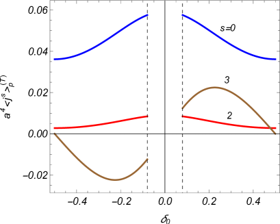
Figure 1: The thermal charge and current densities in the model with $D=4$ as functions of fractional parts of the ratio of magnetic fluxes to the flux quantum. The graphs are plotted for $r/w=0.5$, $L/w=1$, $wT=1$, $w\mu=0.5$, $q=2.5$. For the left panel $\delta_{0}=1/3$ and for the right one $\alpha_{0}=0.2$.

4 Special cases

4.1 Zero angular deficit

Let us consider some special cases of general formula (3.40). In the absence of the cosmic string and magnetic flux one has $q=1$ and $\alpha_{0}=0$ and we will denote the corresponding current density by $\left\langle j^{s}\right\rangle_{0}^{(T)}$. By taking into account that ${\mathcal{J}}_{2}(1,0,z)=0$ we see that the azimuthal current density vanishes, $\left\langle j^{2}\right\rangle_{0}^{(T)}=0$. For the charge and axial current densities, by using ${\mathcal{J}}_{0}(1,0,z)=1$, we get

$$\left\langle j^{s}\right\rangle_{0}^{(T)} = \frac{4e}{\pi^{\frac{D}{2}}}w\left(\frac{w}{a}\right)^{D+1}\int_{0}^{\infty}du\,u^{\frac{D}{2}}\frac{I_{\nu}(2w^{2}u)}{e^{2w^{2}u}}$$ (4.1)

$$\times\left(\frac{-L}{\pi}\partial_{\delta_{0}}\right)^{\delta_{s3}}F_{1}\left(\delta_{0},L^{2}u\right)\left(2\partial_{{\mu}}\right)^{\delta_{s0}}F_{2}\left(\beta{\mu},\beta^{2}u\right)\ ,$$

for $s=0,3$. In the absence of planar angle deficit, $q=1$, the expressions for the functions ${\mathcal{J}}_{s}(q,\alpha_{0},z)$ are simplified to

$${\mathcal{J}}_{0}(1,\alpha_{0},z) = 1-\frac{2}{\pi}\sin\left(\pi|\alpha_{0}|\right)\int_{0}^{\infty}dy\ \frac{e^{-2z\cosh^{2}y}}{\cosh y}\cosh\left[\left(1-2|\alpha_{0}|\right)y\right]\ ,$$

$${\mathcal{J}}_{2}(1,\alpha_{0},z) = \frac{4}{\pi}\sin\left(\pi\alpha_{0}\right)\int_{0}^{\infty}dy\ e^{-2z\cosh^{2}{y}}\sinh\left[\left(1-2|\alpha_{0}|\right)y\right]\sinh y.$$ (4.2)

The parts coming from the integral terms in (4.2) correspond to the contribution of the magnetic flux $\Phi_{2}$.

4.2 Zero chemical potential

For the zero chemical potential, ${\mu}{=0}$, the thermal charge density vanishes $\left\langle j^{0}\right\rangle^{(T)}=0$ as a consequence of the cancellation between the contributions coming from the particles and antiparticles. The expressions for the thermal azimuthal and axial current densities are obtained from (3.40) taking $F_{2}\left(0,u\right)=\sum_{j=1}^{\infty}e^{-j^{2}u}$. Another expression for $F_{2}\left(0,u\right)$ follows from (3.19). An equivalent representation is obtained by substituting in (3.40) the expression (3.15). The $u$-integral is evaluated by using the formula [53]

$$\int_{0}^{\infty}dx\,x^{D/2}e^{-bx}I_{\nu}(x)=\sqrt{\frac{2}{\pi}}Z_{\nu}^{D}(b),\;b>1,$$ (4.3)

with the function in the right-hand side defined by

$$Z_{\nu}^{D}(u)=e^{-i\pi/2(D+1)}\frac{Q_{\nu-1/2}^{\frac{D+1}{2}}(u)}{(u^{2}-1)^{\frac{D+1}{4}}}\ ,$$ (4.4)

where $Q_{\gamma}^{\mu}(u)$ represents the associated Legendre function of the second kind [54]. The current densities are presented as

$$\left\langle j^{s}\right\rangle^{(T)} = \frac{4ea^{-D-1}}{\left(2\pi\right)^{\frac{D+1}{2}}}\left(\frac{-L}{\pi}\partial_{\delta_{0}}\right)^{\delta_{s3}}\sideset{}{{}^{\prime}}{\sum}_{l=0}^{\infty}\cos\left(2\pi l\delta_{0}\right)$$ (4.5)

$$\times\sum_{j=1}^{\infty}\left[2\sideset{}{{}^{\prime}}{\sum}_{k=0}^{[q/2]}A_{k}^{(s)}Z_{\nu}^{D}\left(u_{jkl}\right)-\frac{q}{\pi}\int_{0}^{\infty}dy\ \frac{h_{s}(q,\alpha_{0},y)Z_{\nu}^{D}\left(u_{jyl}\right)}{\cosh(qy)-\cos(q\pi)}\right]\,,$$

for $s=2,3$. Here, we have defined

$$u_{jkl} = 1+\frac{j^{2}\beta^{2}}{2w^{2}}+\frac{l^{2}L^{2}}{2w^{2}}+2\rho^{2}s_{k}^{2},$$

$$u_{jyl} = 1+\frac{j^{2}\beta^{2}}{2w^{2}}+\frac{l^{2}L^{2}}{2w^{2}}+2\rho^{2}\cosh^{2}(y/2)\ .$$ (4.6)

In (4.5) and in what follows $h_{3}(q,\alpha_{0},y)=h_{0}(q,\alpha_{0},y)$ and

$$A_{k}^{(s)} = \cos\left(2\pi k\alpha_{0}\right),\;s=0,3,$$ (4.7)

$$A_{k}^{(2)} = \sin{(2\pi k/q)}\sin\left(2\pi k\alpha_{0}\right).$$

The current densities in the geometry with decompactified $z$-coordinate are obtained from (4.5) in the limit $L\rightarrow\infty$. In this limit the axial current density vanishes and in the expression for the azimuthal current density the contribution of the term with $l=0$ survives only:

$$\left\langle j^{2}\right\rangle_{L=\infty}^{(T)}=\frac{2ea^{-D-1}}{\left(2\pi\right)^{\frac{D+1}{2}}}\sum_{j=1}^{\infty}\left[2\sideset{}{{}^{\prime}}{\sum}_{k=0}^{[q/2]}A_{k}^{(2)}Z_{\nu}^{D}\left(u_{jk0}\right)-\frac{q}{\pi}\int_{0}^{\infty}dy\ \frac{h_{2}(q,\alpha_{0},y)Z_{\nu}^{D}\left(u_{jy0}\right)}{\cosh(qy)-\cos(q\pi)}\right].$$ (4.8)

The expression for the total azimuthal current density in this special case is obtained from (4.8) by the replacement $\sum_{j=1}^{\infty}\rightarrow\sideset{}{{}^{\prime}}{\sum}_{j=0}^{\infty}$ and the part with $j=0$ will correspond to the vacuum current. As before, the prime on the sign of the summation means that the $j=0$ term is taken with coefficient 1/2.

4.3 Conformally coupled massless field

Another special case when the expressions for the components of the current density are simplified corresponds to a conformally coupled massless field. In this case one has $\nu=1/2$ and, by taking into account that $I_{1/2}(x)=\sqrt{2/\pi x}\sinh x$, the current density is presented as

$$\left\langle j^{s}\right\rangle^{(T)}=\left(w/a\right)^{D+1}\left\langle j^{s}\right\rangle_{\mathrm{(M,b)}}^{(T)},$$ (4.9)

where

$$\left\langle j^{s}\right\rangle_{\mathrm{(M,b)}}^{(T)} = \frac{2e}{\pi^{\frac{D+1}{2}}}\int_{0}^{\infty}du\,u^{\frac{D-1}{2}}\left(1-e^{-4w^{2}u}\right){\mathcal{J}}_{s}(q,\alpha_{0},2ur^{2})$$ (4.10)

$$\times\left(-\frac{L}{\pi}\partial_{\delta_{0}}\right)^{\delta_{s3}}F_{1}\left(\delta_{0},L^{2}u\right)\left(2\partial_{{\mu}}\right)^{\delta_{s0}}F_{2}\left(\beta{\mu},\beta^{2}u\right).$$

For a conformally coupled scalar field the problem under consideration is conformally related to the problem with a cosmic string in the Minkowski bulk described by the line element

$$ds_{\mathrm{M}}^{2}=dt^{2}-dr^{2}-r^{2}d\phi^{2}-dw^{2}-dz^{2}-\sum_{i=5}^{D}(dx^{i})^{2}\ ,$$ (4.11)

with compactified $z$-coordinate and with an additional planar boundary at $w=0$ on which the scalar field obeys Dirichlet boundary condition, $\varphi|_{w=0}=0$. The boundary $w=0$ in the Minkowskian problem is the conformal image of the AdS boundary. The expectation value (4.10) is the finite temperature contribution to the current density in the Minkowskian problem and (4.9) is the standard relation between the expectation values in two conformally related problems. The part in (4.10) coming from the first term in $1-e^{-4w^{2}u}$ corresponds to the charge density for a massless scalar field in the Minkowskian problem when the boundary at $w=0$ is absent (we will denote that part by $\left\langle j^{0}\right\rangle_{\mathrm{(M)}}^{(T)}$) and the contribution coming from the second term is induced by the Dirichlet boundary at $w=0$.

The expression in the right-hand side of (4.10) is further transformed by using the representations (3.16), (3.18), (3.22) and (3.34). The integral over $u$ in (4.10) is expressed in terms of the modified Bessel function $K_{\nu}(x)$ and for the thermal current density we obtain

$$\left\langle j^{s}\right\rangle_{\mathrm{(M,b)}}^{(T)} = \frac{2e}{\left(2\pi\right)^{\frac{D}{2}}L}\left(\frac{-L}{\pi}\partial_{\delta_{0}}\right)^{\delta_{s3}}\left(2\partial_{{\mu}}\right)^{\delta_{s0}}\sum_{l=-\infty}^{\infty}|\tilde{k}_{l}|^{D}\sum_{j=1}^{\infty}\cosh\left(j\beta{\mu}\right)$$ (4.12)

$$\times\sum_{n=0,1}(-1)^{n}\left[2\sideset{}{{}^{\prime}}{\sum}_{k=0}^{[q/2]}A_{k}^{(s)}f_{\frac{D}{2}}\left(|\tilde{k}_{l}|\sqrt{j^{2}\beta^{2}+4r^{2}s_{k}^{2}+4nw^{2}}\right)\right.$$

$$\left.-\frac{q}{\pi}\int_{0}^{\infty}dy\ \frac{f_{\frac{D}{2}}\left(|\tilde{k}_{l}|\sqrt{j^{2}\beta^{2}+4r^{2}\cosh^{2}(y/2)+4nw^{2}}\right)}{\cosh(qy)-\cos(q\pi)}h_{s}(q,\alpha_{0},y)\right],$$

where

$$f_{\nu}(x)=x^{-\nu}K_{\nu}(x).$$ (4.13)

In the expression for the axial current density we can use the relation

$$\frac{-L}{\pi}\partial_{\delta_{0}}\left[|\tilde{k}_{l}|^{D}f_{\frac{D}{2}}(|\tilde{k}_{l}|x)\right]=2\tilde{k}_{l}|\tilde{k}_{l}|^{D-2}f_{\frac{D}{2}-1}(|\tilde{k}_{l}|x)$$ (4.14)

The $n=0$ term in (4.12) presents the current density $\left\langle j^{s}\right\rangle_{\mathrm{(M)}}^{(T)}$ and the part with $n=1$ is induced by the boundary at $w=0$. Note that $\left\langle j^{s}\right\rangle_{\mathrm{(M,b)}}^{(T)}|_{w=0}=0$. This result is a consequence of Dirichlet boundary condition imposed on the scalar field at $w=0$.

5 Asymptotic analysis

5.1 Small and high temperatures

Let us consider the behavior of the thermal currents in asymptotic regions of the parameters. For small temperatures one has ${\beta/w\gg 1}$ and the dominant contribution to the integral over $x$ in (3.40) comes from the region with small $x$. By using the asymptotic (3.42) for the function $F_{1}(\delta_{0},u)$ and the asymptotic (3.43) for ${\mathcal{J}}_{s}(q,\alpha_{0},z)$, we get

$$\left\langle j^{s}\right\rangle^{(T)} \approx \frac{eq(w/a)^{D+1}w^{2\nu+1}r^{2q|\alpha_{0}|-2\delta_{s2}}\left(q\alpha_{0}\right)^{\delta_{s2}}T}{2^{\nu+q|\alpha_{0}|+1}\left(2\pi\right)^{\frac{D}{2}-1}\Gamma\left(\nu+1\right)\Gamma(q|\alpha_{0}|+1)}$$ (5.1)

$$\times\left(2\partial_{{\tilde{\mu}}}\right)^{\delta_{s0}}\left(-\frac{\partial_{\delta_{0}}}{\pi}\right)^{\delta_{s3}}\left(E_{0}T\right)^{\frac{D}{2}+\nu+q|\alpha_{0}|-\delta_{s2}}\sum_{j=1}^{\infty}\frac{e^{-j\left(E_{0}-|{\mu|}\right)/T}}{j^{\frac{D}{2}+\nu+q|\alpha_{0}|+1-\delta_{s2}}}.$$

If in addition $T\ll E_{0}-{\mu}$, the $j=1$ term dominates and the components of the current density tend to zero like $T^{D/2+\nu+q|\alpha_{0}|}e^{-(E_{0}-{\mu)/T}}$.

At large temperatures, $wT\gg 1$, the discussion of the asymptotic behavior differs for the charge density and currents. That is related to the different behavior of the integrand at the upper limit of integration in (3.40). For the charge density, we introduce in (3.17) a new variable $x=\beta^{2}u$ and expand the functions with large arguments $x/\beta^{2}$. By using (3.41) for $F_{1}(\delta_{0},u)$, the leading term is expressed as

$$\left\langle j^{0}\right\rangle^{(T)}\approx\left(\frac{w}{a}\right)^{D+1}\frac{2e{\mu}}{\pi^{\frac{D+1}{2}}}\Gamma\left(\frac{D+1}{2}\right)\zeta\left(D-1\right){T}^{D-1}.$$ (5.2)

For the components $s=2,3$ we use the asymptotic (3.42) for the function $F_{2}\left(\beta{\mu},\beta^{2}u\right)$. To the leading order this gives

$$\left\langle j^{s}\right\rangle^{(T)} \approx \frac{2eTw}{\pi^{\frac{D-1}{2}}}\left(\frac{w}{a}\right)^{D+1}\int_{0}^{\infty}du\,u^{\frac{D-1}{2}}\frac{I_{\nu}(2w^{2}u)}{e^{2w^{2}u}}\exp\left(\frac{{\mu}^{2}}{4u}\right)$$ (5.3)

$$\times{\mathcal{J}}_{s}(q,\alpha_{0},2ur^{2})\left(\frac{-L}{\pi}\partial_{\delta_{0}}\right)^{\delta_{s3}}F_{1}\left(\delta_{0},L^{2}u\right).$$

It is of interest to compare the obtained results with the thermal charge density in the Minkowski spacetime. For a scalar field with mass $m$ and the chemical potential ${\mu}$ the expectation value of the charge density is given by (see, for example, [45])

$$\left\langle j^{0}\right\rangle_{\mathrm{(M)}}^{(T)}=\frac{4e\beta m^{D+1}}{(2\pi)^{\frac{D+1}{2}}}\sum_{j=1}^{\infty}j\sinh(j{\mu}\beta)f_{\frac{D+1}{2}}(j\beta m),$$ (5.4)

where $f_{\nu}(x)$ is defined by (4.13). At high temperatures $T\gg m$ for the leading order term we get

$$\left\langle j^{0}\right\rangle_{\mathrm{(M)}}^{(T)}\approx\frac{2e{\mu}}{\pi^{\frac{D+1}{2}}}\Gamma\left(\frac{D+1}{2}\right)\zeta\left(D-1\right)T^{D-1}.$$ (5.5)

Comparing with (5.2), we see the relation $\left\langle j^{0}\right\rangle^{(T)}\approx(w/a)^{D+1}\left\langle j^{0}\right\rangle_{\mathrm{(M)}}^{(T)}$ at high temperatures. At high temperatures the dominant contribution to the charge density comes from the field fluctuations with small wavelengths and the effects of the curvature are small.

Figures 2 and 3 display the thermal charge and current densities as functions of the temperature in the $D=4$ model for $r/w=0.5$, $L/w=1$, $w\mu=0.5$, $q=1.5$, $\alpha_{0}=\delta_{0}=0.2$. The full and dashed curves correspond to minimally and conformally coupled fields and the numbers near the curves are the values of $ma$. The numerical data presented in figures confirm the features clarified by the asymptotic analysis. Liner dependence for the azimuthal and axial current densities and stronger increase of the charge density at high temperatures are clearly seen.

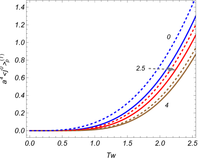
Figure 2: The charge density for minimally (full curves) and conformally (dashed curves) coupled scalar fields in the model with $D=4$ versus the temperature for fixed values $r/w=0.5$, $L/w=1$, $w\mu=0.5$, $q=1.5$, $\alpha_{0}=\delta_{0}=0.2$. The graphs are plotted for different values of the product $ma$.

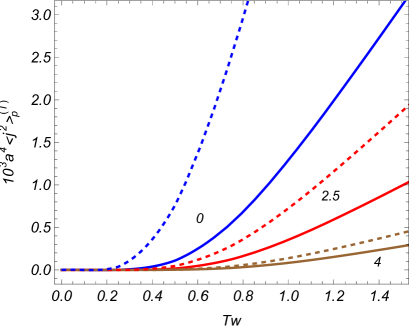
Figure 3: The same as in figure 2 for the azimuthal (left panel) and axial (right panel) current densities.

5.2 Asymptotics with respect to the compactification length

For small values of the compactification length, $L/w\ll 1$, we use the asymptotic (3.42) for the function $F_{1}(\delta_{0},u)$. The dominant contribution to the $u$-integral in (3.40) comes from the region $u\gtrsim\pi^{2}|\delta_{0}|^{2}/L^{2}$. In that region $u$ is large and we use the corresponding asymptotic for the integrand. The integral over $u$ is expressed in terms of the modified Bessel function and we get

$$\left\langle j^{s}\right\rangle^{(T)} \approx \frac{2eE_{0}^{D}}{\left(2\pi\right)^{\frac{D}{2}}L}\left(\frac{w}{a}\right)^{D+1}\left(\frac{-L}{\pi}\partial_{\delta_{0}}\right)^{\delta_{s3}}\left(2\partial_{{\tilde{\mu}}}\right)^{\delta_{s0}}\cosh\left(\beta{\mu}\right)$$ (5.6)

$$\left[2\sideset{}{{}^{\prime}}{\sum}_{k=0}^{[q/2]}A_{k}^{(s)}f_{\frac{D}{2}}(E_{0}\sqrt{\beta^{2}+4r^{2}s_{k}^{2}})\right.$$

$$\left.-\frac{q}{\pi}\int_{0}^{\infty}dy\ \frac{f_{\frac{D}{2}}(E_{0}\sqrt{\beta^{2}+4r^{2}\cosh^{2}(y/2)})}{\cosh(qy)-\cos(q\pi)}h_{s}(q,\alpha_{0},y)\right].$$

If in addition, $\beta/L,r/L\gg 1$, for the components with $s=0,3$ the main contribution in (5.6) comes from the term $k=0$ and they behave as $\left\langle j^{s}\right\rangle^{(T)}\propto e^{-E_{0}\beta}/L^{\frac{D+1}{2}}$. For the component $\left\langle j^{2}\right\rangle^{(T)}$ one has $A_{0}^{(2)}=0$ and an additional exponential suppression factor is present coming from the part in the square brackets of (5.6). Hence, for $\delta_{0}>0$ and for small $L$ we have an exponential suppression for all the components.

For $\delta_{0}=0$ we should also put $\mu=0$. In this case the only nonzero component corresponds to the azimuthal current density. In order to find the asymptotic for $L/w\ll 1$ we use the expression (4.5) for $s=2$ and $\delta_{0}=0$. The dominant contribution to the series over $l$ comes from large values of $l$ and to the leading order we can replace the summation by the integration: $\sum_{l=0}^{\infty}\rightarrow\int_{0}^{\infty}dl$. The resulting integral is evaluated by using the formula

$$\int_{0}^{\infty}du\,Z_{\nu}^{D}\left(b^{2}+u^{2}\right)=\frac{\sqrt{\pi}}{2}Z_{\nu}^{D-1}(b^{2}).$$ (5.7)

This formula is obtained by using the integral representation for the function $Z_{\nu}^{D}\left(x\right)$ given by (4.3). In this way we can see that

$$\left\langle j^{2}\right\rangle^{(T)}|_{\delta_{0}=0}\approx\frac{w}{aL}\left\langle j^{2}\right\rangle_{D}^{(T)},$$ (5.8)

where $\left\langle j^{2}\right\rangle_{D}^{(T)}$ is the azimuthal current density for a scalar field with zero chemical potential in a $D$-dimensional AdS spacetime, obtained from the geometry described above excluding the $z$-coordinate. The corresponding expression is obtained from (4.8) by the replacement $D\rightarrow D-1$.

Considering the asymptotic for large values of the compactification length, we note that for a given value of the chemical potential the maximal length of the compact dimension, $L_{m}$, is determined by the condition (2.18): $L_{m}=2\pi|\delta_{0}|/|\mu|$. For the zero chemical potential, ${\mu}{=0}$, the thermal charge density vanishes. Denoting $\left\langle j^{s}\right\rangle_{L=\infty}^{(T)}=\lim_{L\rightarrow\infty}\left\langle j^{s}\right\rangle^{(T)}$ for the components $s=2,3$, we can see that $\left\langle j^{3}\right\rangle_{L=\infty}^{(T)}=0$ and

$$\left\langle j^{2}\right\rangle_{L=\infty}^{(T)}=\frac{ea^{-D-1}}{\left(2\pi\right)^{\frac{D}{2}}}\int_{0}^{\infty}dx\,x^{\frac{D}{2}}\frac{I_{\nu}(x)}{e^{x}}{\mathcal{J}}_{2}(q,\alpha_{0},x\rho^{2})F_{2}\left(0,\beta^{2}x/(2w^{2}\right)).$$ (5.9)

This result gives the current density for a cosmic string in locally AdS bulk where the $z$-direction has uncompactified topology $R^{1}$. In order to find the next terms in the expansion over $1/L$, we use the representation (3.40) with the function $F_{1}\left(\delta_{0},L^{2}u\right)$ from (3.15) and with

$$F_{2}\left(0,\beta^{2}u\right)=\frac{1}{\beta}\sqrt{\frac{\pi}{u}}\sideset{}{{}^{\prime}}{\sum}_{j=0}^{\infty}e^{-\pi^{2}j^{2}/(\beta^{2}u)}-\frac{1}{2}.$$ (5.10)

The leading contribution to the difference $\left\langle j^{s}\right\rangle^{(T)}-\left\langle j^{s}\right\rangle_{L=\infty}^{(T)}$ comes from the term $j=0$ in (5.10) and we get

$$\left\langle j^{s}\right\rangle^{(T)} \approx \left\langle j^{s}\right\rangle_{L=\infty}^{(T)}+\frac{2eqw^{2\nu+1}r^{2q|\alpha_{0}|}\left(w/a\right)^{D+1}T}{\pi^{\frac{D-1}{2}}\Gamma\left(\nu+1\right)\Gamma(q|\alpha_{0}|+1)}\left(\frac{q\alpha_{0}}{2r^{2}}\right)^{\delta_{s2}}$$ (5.11)

$$\times\left(\frac{-L}{\pi}\partial_{\delta_{0}}\right)^{\delta_{s3}}\sum_{l=1}^{\infty}\cos\left(2\pi l\delta_{0}\right)\frac{\Gamma\left(\frac{D+1}{2}+\nu+q|\alpha_{0}|-\delta_{s2}\right)}{\left(lL\right)^{D+1+2\left(\nu+q|\alpha_{0}|-\delta_{s2}\right)}}.$$

for $s=2,3$.

For $D=4$ minimally coupled massless scalar field, the dependence of the charge and current densities on the proper length of the compact dimension is depicted in Figures 4 and 5. The graphs are plotted for $r/w=0.5$, $w\mu=0.5$, $q=1.5$, $\alpha_{0}=0.25$, $\delta_{0}=1/3$ and for different values of the temperature (the numbers near the curves). In accordance with the asymptotic analysis, all the components tend to zero for small values of the compactification length.

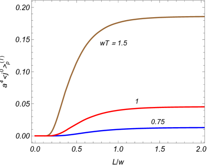
Figure 4: The charge density for a minimally coupled scalar field as a function of the compactification length in the $D=4$ model. The graphs are plotted for $r/w=0.5$, $w\mu=0.5$, $q=1.5$, $\alpha_{0}=0.25$, $\delta_{0}=1/3$ and the numbers near the curves are the respective values of the temperature.

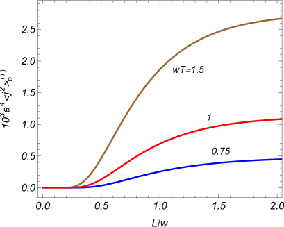
Figure 5: The same as in figure 4 for the azimuthal (left panel) and axial (right panel) current densities.

5.3 Small and large distances from cosmic string

In order to find the asymptotic of the thermal current density near the cosmic string, $\rho\ll 1$, we use the expression (3.40) and the approximation (3.43) for the function ${\mathcal{J}}_{s}(q,\alpha_{0},2ur^{2})$. The latter shows that $\left\langle j^{s}\right\rangle^{(T)}\propto r^{2q|\alpha_{0}|-2\delta_{s2}}$ for $r\rightarrow 0$. Hence, for $\alpha_{0}\neq 0$ the charge and axial current densities vanish on the string. The contravariant component of the azimuthal current density vanishes on the string for $|\alpha_{0}|>1/q$ and diverges for $|\alpha_{0}|<1/q$. Note that the physical component of the azimuthal current density behaves as $\left\langle j^{2}\right\rangle_{\mathrm{p}}^{(T)}\propto r^{2q|\alpha_{0}|-1}$.

At large distances from the string, $\rho\gg 1$, one gets $\lim_{r\rightarrow\infty}\left\langle j^{s}\right\rangle^{(T)}=\left\langle j^{s}\right\rangle_{0}^{(T)}$, where the components with $s=0,3$ are given by (4.1) and $\left\langle j^{2}\right\rangle_{0}^{(T)}=0$. The effects induced by cosmic string and magnetic flux are encoded in the difference $\left\langle j^{s}\right\rangle^{(T)}-\left\langle j^{s}\right\rangle_{0}^{(T)}$. For $\rho\gg 1$ the dominant contribution to the integral over $u$ in (3.40) comes from the region with small values of $u$. By using the corresponding asymptotics (3.42), we can see that

$$\left\langle j^{s}\right\rangle^{(T)} = \left\langle j^{s}\right\rangle_{0}^{(T)}+\frac{2eTw^{D+2\nu+2}{\mu}^{\delta_{s0}}}{\pi^{\frac{D}{2}-1}\Gamma\left(\nu+1\right)a^{D+1}L}\left(\frac{2\pi}{L}\delta_{0}\right)^{\delta_{s3}}\left(\frac{E_{0}^{2}-{\mu}^{2}}{2}\right)^{\frac{D}{2}+\nu-1+\delta_{s2}}$$ (5.12)

$$\times\left[2\sideset{}{{}^{\prime}}{\sum}_{k=1}^{[q/2]}A_{k}^{(s)}f_{\frac{D}{2}+\nu-1+\delta_{s2}}\left(2rs_{k}\sqrt{E_{0}^{2}-{\mu}^{2}}\right)\right.$$

$$\left.-\frac{q}{\pi}\int_{0}^{\infty}dy\ \frac{f_{\frac{D}{2}+\nu-1+\delta_{s2}}\left(2r\sqrt{E_{0}^{2}-{\mu}^{2}}\cosh(y/2)\right)}{\cosh(qy)-\cos(q\pi)}h_{s}(q,\alpha_{0},y)\right],$$

If in addition $r\sqrt{E_{0}^{2}-{\mu}^{2}}\gg 1$, the cosmic string induced contribution $\left\langle j^{s}\right\rangle^{(T)}-\left\langle j^{s}\right\rangle_{0}^{(T)}$ decays as $e^{-2rs_{1}\sqrt{E_{0}^{2}-{\mu}^{2}}}/r^{(D-1)/2+\nu+\delta_{s2}}$ for $q\geq 2$ and like $e^{-2r\sqrt{E_{0}^{2}-{\mu}^{2}}}/r^{(D-1)/2+\nu+\delta_{s2}}$ for $1<q<2$. As it has been already discussed in Section 3, the total charge, per unit volume in the subspace $(\mathbf{x}_{\parallel},w)$, induced by the presence of the cosmic string is finite and is given by the expression (3.28). This finiteness is a consequence of the exponential decrease of the related charge density at large distances from the string.

The dependence of the thermal charge and current densities on the proper distance from the cosmic string is displayed in Figures 6 and 7. The graphs are plotted for $D=4$ minimally coupled massless field for fixed values $L/w=1$, $Tw=1$, $w\mu=0.5$, $\alpha_{0}=0.25$, $\delta_{0}=1/3$ and the numbers near the curves correspond to the values of the parameter $q$. In accordance with the asymptotic analysis given above, the components with $s=0,3$ vanish on the string. For the parameters we have taken in Figure 7 and for $q=2$ one has $2q|\alpha_{0}|=1$ and the azimuthal component tends to finite nonzero value on the cosmic string. The graphs on the left panel of Figure 7 also confirm the features described by the asymptotic analysis on that the physical component of the thermal contribution to the azimuthal current density vanishes on the string for $|\alpha_{0}|>1/(2q)$ and diverges for $|\alpha_{0}|<1/(2q)$.

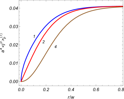
Figure 6: The dependence of the thermal charge density on the proper distance from the cosmic string for a minimally coupled $D=4$ scalar field. For the parameters we have taken $L/w=1$, $Tw=1$, $w\mu=0.5$, $\alpha_{0}=0.25$, $\delta_{0}=1/3$ and the numbers near the curves present the values of $q$.

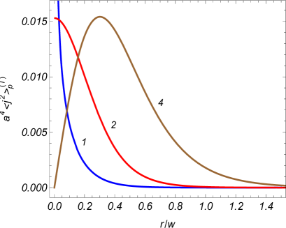
Figure 7: The same as in figure 6 for the azimuthal (left panel) and axial (right panel) current densities.

Before we summarize the main results of the paper it is worth pointing out about some potential applications and generalizations. In Introduction we have mentioned two mechanisms for the production of cosmic string type topological defects: formation of cosmic strings as a result of symmetry breaking phase transitions in the expanding early universe and formation of string-type linear structures in brane inflation models. The defects produced in the second mechanism can be either fundamental strings or one-dimensional branes (F- and D-strings, respectively). Their bound states can be formed as well. The linear structures formed in brane inflation models may have different sizes and cosmologically extended ones become cosmic superstrings. The investigations of the effects induced by those structures in the AdS spacetime are partly motivated by that the related geometry appears as ground state in superstring theories and as a bulk geometry in braneworld models. An additional motivation comes from the AdS/CFT correspondence: the initial version of that correspondence states a duality between IIB string theory on the AdS bulk and $\mathcal{N}=4$ super-Yang-Mills (SYM) theory on its boundary. The defect we have discussed in the present paper can be considered as a simple realization of D$p$-brane with $p=D-2$. The geometry of the core is described by the line element (2.2) that corresponds to $(D-1)$-dimensional AdS spacetime (locally AdS in the model with compactified $z$-direction). The vacuum polarization and the Casimir forces for planar D$p$-branes with $p=D-1$, orthogonal to the AdS boundary, have been discussed in Refs. [52, 56]. In the problem under consideration and for $D=3$ one has a linear defect in the AdS bulk and a point-like defect in the dual theory on the AdS boundary. Note that the gravitational field of the point mass in 3-dimensional spacetime is described by conical geometry (see, for example, [57]). That geometry also appears in the effective long-wavelength description for a number of planar condensed matter systems (examples are the graphene nanocones). In Ref. [58] the AdS₄/CFT₃ correspondence have been used to evaluate the Green function for scalar operators in 3-dimensional conical spacetime. For spatial dimension $D=4$ the defect in the bulk is 2-dimensional and the corresponding counterpart in the dual theory is the standard straight cosmic string (in the model with $-\infty<z<+\infty$) or a cosmic string compactified along its axis (model with compactified $z$-direction). Hence, the results described in the present paper can be used to investigate the thermal effects of cosmic string type defects in the dual theory on the AdS boundary by using the AdS/CFT map.

We have considered a thermal field theory in the background geometry described by the metric (2.1). In the context of the AdS/CFT correspondence, the dual theory is a thermal field theory with the line element $ds_{\mathrm{CFT}}^{2}=dt^{2}-\gamma_{ij}dx^{i}dx^{j}$, where $\gamma_{ij}dx^{i}dx^{j}=dr^{2}+r^{2}d\phi^{2}+dz^{2}+d\mathbf{x}_{\parallel}^{2}$. Note that for the geometry with decompactified $z$-coordinate and for scale invariant dual theories the only dimensionful parameter is the temperature. The latter can be changed by a scaling and there are no phase transitions in those theories. An example is the $\mathcal{N}=4$ SYM on $R^{3}$ as the dual theory in the initial version of the AdS/CFT correspondence. The compactification of the $z$-coordinate introduces an additional length scale in the model and the phase transitions may take place (see, for example, the discussion in Ref. [59] for $\mathcal{N}=4$ SYM). It is important to note that the AdS counterpart of the boundary theory is not unique. As alternatives to the pure AdS spacetime, AdS black holes with different geometries of the horizon have been considered in the literature (for black hole solutions in AdS spacetime with different topologies of the horizon see, e.g., Refs. [60, 61]). The corresponding solution with the planar horizon, most appropriate in the problem under consideration, is given by

$$ds_{\mathrm{BH}}^{2}=\frac{a^{2}}{w^{2}}\left\{\left[1-\left(\frac{w}{w_{\mathrm{H}}}\right)^{D}\right]dt^{2}-\frac{dw^{2}}{1-\left(w/w_{\mathrm{H}}\right)^{D}}-\gamma_{ij}dx^{i}dx^{j}\right\},$$ (5.13)

where the hypersurface $w=w_{\mathrm{H}}$, with

$$w_{\mathrm{H}}=\left[\frac{(D-1)a^{D-1}}{16\pi G\rho_{m}}\right]^{1/D},$$ (5.14)

corresponds to the horizon. Here, $G$ is the gravitational constant in $(D+1)$-dimensional spacetime and $\rho_{m}$ is the mass per unit volume of the subspace with the line element $\gamma_{ij}dx^{i}dx^{j}$. For $0\leq\phi\leq 2\pi$, introducing a new radial coordinate $\rho=a^{2}/w$ and the Cartesian coordinates in the subspace $(r,\phi)$, this solution is reduced to the one given, for example, in Ref. [61]. In the case $0\leq\phi\leq\phi_{0}<2\pi$ the metric (5.13) describes a combination of AdS planar black hole with a generalized cosmic string type topological defect crossing the black hole horizon. In the context of the AdS/CFT correspondence, two geometries described by (2.3) and (5.13) may correspond to two different phases of the dual theory. The phase transition in the dual theory is interpreted in terms of the Hawking-Page phase transition in the AdS bulk [36].

The thermal charge and current densities will also appear for a quantum charged scalar field propagating in the background of the black hole geometry (5.13). At large distances from the horizon, $w/w_{\mathrm{H}}\ll 1$, corresponding to points near the AdS boundary, the geometry we have considered in the present paper is the leading order approximation to the line element (5.13). The expressions for the charge and current densities given above will give the leading terms in the respective asymptotic expansions with respect to the small ratio $w/w_{\mathrm{H}}$. Another limiting region where the geometry (5.13) is simplified corresponds to points near the black hole horizon, $1-w/w_{\mathrm{H}}\ll 1$. Expanding the metric tensor and introducing new coordinates

$$\tau=\frac{Dt}{2w_{\mathrm{H}}},\;\bar{u}=-\frac{2a}{\sqrt{D}}\sqrt{1-\frac{w}{w_{\mathrm{H}}}},\;\left(\bar{r},\bar{z},\mathbf{\bar{x}}_{\parallel}\right)=\frac{a}{w_{\mathrm{H}}}\left(r,z,\mathbf{x}_{\parallel}\right),$$ (5.15)

the line element (5.13) is approximated by

$$ds_{\mathrm{BH}}^{2}\approx\bar{u}^{2}d\tau^{2}-d\bar{u}^{2}-d\bar{r}^{2}-\bar{r}^{2}d\phi^{2}-d\bar{z}^{2}-d\mathbf{\bar{x}}_{\parallel}^{2}.$$ (5.16)

The right-hand side corresponds to the $(D+1)$-dimensional Rindler spacetime with compact $z$-direction and in the presence of a generalized cosmic string. Note that the length of the compact dimension $\bar{z}$ is given by $\bar{L}=aL/w_{\mathrm{H}}$ and it depends on the location of the horizon. The simple form of the near-horizon metric allows to obtain closed analytic expressions for the expectation values of the charge and current densities. In the absence of the cosmic string, the corresponding vacuum expectation values in Rindler spacetime with an arbitrary number of toroidally compact dimensions have been recently discussed in [62].

6 Conclusions

We have investigated combined effects of background gravitational field, nontrivial spatial topology and finite temperature on the expectation values of the charge and current densities for a massive scalar field with general curvature coupling. Motivated by high symmetry and by importance in recent theoretical constructions, as a bulk geometry we have chosen the locally AdS spacetime. Two sources of nontrivial topology are considered. The first one corresponds to a defect that is a generalization of a cosmic string in the presence of extra dimensions and the second one comes from the compactification of a spatial dimension in Poincaré coordinates. We have started the investigation from the Hadamard two-point function. The finite temperature part of that function in the problem at hand is expressed as (2.16) with particle and antiparticle contributions coming from the terms with $u=+$ and $u=-$. The evaluation of various physical characteristics bilinear in the field is based on the Hadamard function. An important difference from the Minkowskian bulk is related to the upper bound of the chemical potential given by (2.18). It does not depend on the field mass and becomes zero in the decompactification limit. This qualitative difference is related to that the mass does not enter in the expression for the energy of the modes. We have also evaluated the bulk-to-boundary propagator for a scalar field that plays an important role in the interpretations of the bulk quantities in terms of the boundary field theory in the context of the AdS/CFT correspondence.

As important characteristics for a charged field we have considered the charge and current densities. The vacuum expectation values of those quantities have been considered in a recent publication [25] and here we were mainly concerned with the thermal contributions. The nonzero components correspond to the charge density, azimuthal current density and the current density along the compact dimension (axial current). We note that the nonzero charge density is a pure thermal effect: the corresponding vacuum average is zero. The combined expression for the nonzero components is given by (3.40). As a consequence of the AdS maximal symmetry, the thermal expectation values depend on the parameters having the dimension of length through the ratios like $r/w$, $L/w$. They correspond to the proper distance from the defect and proper length of the compact dimension in the units of the curvature radius. The charge density is an odd function of the chemical potential. It vanishes for zero chemical potential as a result of cancellation between the contributions from particles and antiparticles. The azimuthal and axial currents are even functions of the chemical potential and survive in the limit $\mu=0$. We have considered two types of magnetic fluxes. The first one is confined inside the defect core and another one is interpreted as a flux enclosed by compact dimension. All the components of the current density are periodic functions of those fluxes with the flux quantum being the period. The dependence of the expectation values on the magnetic fluxes appears in the form of two parameters $\alpha_{0}$ and $\delta_{0}$ corresponding to the ratios of the magnetic fluxes to the flux quantum.

Our general results include various special cases. In the absence of the cosmic string the only source of the nontrivial topology is the compactification of the $z$ coordinate and the azimuthal current density becomes zero. The thermal contributions to the charge and axial current densities in this special case are given by (4.1). For the zero chemical potential we have provided alternative representation (4.5) for the azimuthal and axial currents. In this special case we can consider also the decompactification limit $L\rightarrow\infty$. For the nonzero chemical potential one has the maximal value of the compactification length given by $L_{m}=2\pi|\delta_{0}|/|\mu|$. For a conformally coupled massless scalar field the problem at hand is conformally related to the problem of a cosmic string in the Minkowski spacetime with a compact dimension in the presence of a planar Dirichlet boundary orthogonal to the string (see (4.9) and (4.10)). The total charge, per unit volume in the subspace $(\mathbf{x}_{\parallel},w)$, induced by the cosmic string is finite. Its dependence on the parameters of the cosmic string is factorized in a simple form (see (3.28)). Depending on the planar angle deficit and magnetic flux, the presence of the cosmic string can either increase or decrease the total charge.

To clarify the behavior of the expectation values we have considered various asymptotic limits. In the zero temperature limit the thermal densities tend to zero like $T^{D/2+\nu+q|\alpha_{0}|}e^{-(E_{0}-{\mu)/T}}$. The high temperature behavior is different for the charge density and current densities. At high temperatures the influence of the gravitational field and topology on the charge density is subdominant and the leading term coincides with that for the charge density in the Minkowski spacetime with the behavior $\propto T^{D-1}$. The current densities are topology-induced quantities and their behavior at high temperatures is completely different with the linear dependence on the temperature. For $\delta_{0}>0$ all the expectation values are exponentially small for small values of the compactification length. The situation is different in the case $\delta_{0}=0$ when the chemical potential is zero as well. The charge and axial current densities are zero in this case. The leading term in the expansion of the azimuthal current density for small values of $L$ is given by the right-hand side of (5.8), where $\left\langle j^{2}\right\rangle_{D}^{(T)}$ is the azimuthal current density in $D$-dimensional AdS spacetime which is obtained from the geometry we consider excluding the coordinate corresponding to the compact dimension $z$. In the consideration of the decompactification limit for the $z$ direction the chemical potential should be set zero. In the decompactified geometry the charge and axial current densities are zero and the azimuthal current density is given by (5.9). The next-to-leading terms in the azimuthal ($s=2$) and axial ($s=3$) current densities decay like $1/L^{D+1+2(\nu+q|\alpha_{0}|-\delta_{s2})}$. The suppression for the axial component is stronger. Near the cosmic string the thermal contributions to the charge and axial current densities behave like $r^{2q|\alpha_{0}|}$ and they vanish on the cosmic string for $\alpha_{0}\neq 0$. In the same limit the physical azimuthal component behaves as $r^{2q|\alpha_{0}|-1}$. The leading terms in the expansion of the thermal expectation values over the inverse distance from the cosmic string coincide with the corresponding quantities in the geometry where the cosmic string is absent. The next-to-leading terms encode the effects of the cosmic string. For $q\geq 2$, at large distances their decay is described by the factor $e^{-2rs_{1}\sqrt{E_{0}^{2}-{\mu}^{2}}}/r^{(D-1)/2+\nu+\delta_{s2}}$. The suppression factor in the range $1<q<2$ is obtained by the replacement $s_{1}\rightarrow 1$.

The investigation of thermal effects on the AdS bulk may shed light on the phase structure in the boundary theory. We have emphasized the importance of compactification to have phase transitions in scale invariant theories. The confining phase in the boundary gauge theory is mapped onto AdS black hole geometry. Our results approximate the corresponding expectation values around black holes with planar horizons at large distances from the horizon. We have noted that closed analytic expressions can also be obtained for the near-horizon region where the geometry is approximated by Rindler spacetime with a compact dimension in the presence of cosmic string type topological defect.

References

- [1] T. W. Kibble, Topology of cosmic domains and strings, J. Phys. A. 9, 1387 (1976).
- [2] A. Vilenkin and E. P. S. Shellard, Cosmic Strings and Other Topological Defects (Cambridge University Press, Cambridge, England, 1994).
- [3] M. Hindmarsh, Signals of inflationary models with cosmic strings, Prog. Theor. Phys. Suppl. 190, 197 (2011); M. Kawasaki, K. Miyamoto and K. Nakayama, Gravitational waves from kinks on infinite cosmic strings, Phys. Rev.D 81, 103523 (2010); K. S. Virbhadra, Relativistic images of Schwarzschild black hole lensing, Phys. Rev.D 79, 083004 (2009); A. A. Fraisse, C. Ringeval, D. N. Spergel, and F. R. Bouchet, Small-angle CMB temperature anisotropies induced by cosmic strings, Phys. Rev. D 78, 043535 (2008); L. Pogosian and M. Wyman, B-modes from cosmic strings, Phys. Rev. D 77, 083509 (2008); K. S. Virbhadra and G. F. R. Ellis, Schwarzschild black hole lensing, Phys. Rev. D 62, 084003 (2000); A. de Laix, L. M. Krauss and T. Vachaspati, Gravitational lensing signature of long cosmic strings, Phys. Rev. Lett. 79, 1968 (1997); N. Kaiser and A. Stebbins, Microwave anisotropy due to cosmic strings, Nature 310, 391 (1984); A. Vilenkin, Gravitational radiation from cosmic strings, Phys. Lett. B 107, 47 (1981).
- [4] E. J. Copeland, L. Pogosian, and T. Vachaspati, Seeking string theory in the cosmos, Classical Quantum Gravity 28, 204009 (2011).
- [5] D. F. Chernoff and S.-H. Henry Tye, Inflation, string theory and cosmic strings, Int. J. Mod. Phys. D 24, 1530010 (2015).
- [6] S. Bellucci, E. R. Bezerra de Mello, A. de Padua, and A. A. Saharian, Fermionic vacuum polarization in compactified cosmic string spacetime, Eur. Phys. J. C 74, 2688 (2014).
- [7] L. Sriramkumar, Fluctuations in the current and energy densities around a magnetic-flux-carrying cosmic string, Class. Quantum Grav. 18, 1015 (2001).
- [8] Yu. A. Sitenko and N. D. Vlasii, Induced vacuum current and magnetic field in the background of a cosmic string, Class. Quantum Grav. 26, 195009 (2009).
- [9] Yu. A. Sitenko and N. D. Vlasii, Vacuum polarization in graphene with a topological defect, Low Temp. Phys. 34, 826 (2008).
- [10] E.R. Bezerra de Mello, Induced fermionic current densities by magnetic flux in higher dimensional cosmic string spacetime, Class. Quantum Grav. 27, 095017 (2010).
- [11] E. R. Bezerra de Mello, V. B. Bezerra, A. A. Saharian, and H. H. Harutyunyan, Vacuum currents induced by a magnetic flux around a cosmic string with finite core, Phys. Rev. D 91, 064034 (2015).
- [12] E. R. Bezerra de Mello, V. B. Bezerra, A. A. Saharian, and V. M. Bardeghyan, Fermionic current densities induced by magnetic flux in a conical space with a circular boundary, Phys. Rev. D 82, 085033 (2010).
- [13] Yu. A. Sitenko and N. D. Vlasii, Non-Euclidean geometry, nontrivial topology and quantum vacuum effects, Universe 4, 23 (2018).
- [14] S. Bellucci, I. Brevik, A. A. Saharian, and H. G. Sargsyan, The Casimir effect for fermionic currents in conical rings with applications to graphene ribbons, Eur. Phys. J. C 80, 281 (2020).
- [15] E. R. Bezerra de Mello and A. A. Saharian, Vacuum polarization by a cosmic string in de Sitter spacetime, JHEP 04 (2009) 046.
- [16] E. R. Bezerra de Mello and A. A. Saharian, Fermionic vacuum polarization by a cosmic string in de Sitter spacetime, JHEP 08 (2010) 038.
- [17] A. A. Saharian, V. F. Manukyan, and N. A. Saharyan, Electromagnetic vacuum fluctuations around a cosmic string in de Sitter spacetime, Eur. Phys. J. C 77, 478 (2017).
- [18] E. R. Bezerra de Mello and A.A. Saharian, Vacuum polarization induced by a cosmic string in anti-de Sitter spacetime, J. Phys. A 45, 115002 (2012).
- [19] E. R. Bezerra de Mello, E. R. Figueiredo Medeiros, and A. A. Saharian, Fermionic vacuum polarization by a cosmic string in anti-de Sitter spacetime, Class. Quant. Grav. 30, 175001 (2013).
- [20] A. H. Castro Neto, F. Guinea, N. M. R. Peres, K. S. Novoselov, and A. K. Geim, The electronic properties of graphene, Rev. Mod. Phys. 81, 109 (2009).
- [21] E. R. Bezerra de Mello and A. A. Saharian, Topological Casimir effect in compactified cosmic string spacetime, Class. Quant. Grav. 29, 035006 (2012).
- [22] S. Bellucci, E. R. Bezerra de Mello, A. de Padua, and A.A. Saharian, Fermionic vacuum polarization in compactified cosmic string spacetime, Eur. Phys. J. C 74, 2688 (2014).
- [23] E. A. F. Bragança, H. F. Santana Mota, and E. R. Bezerra de Mello, Induced vacuum bosonic current by magnetic flux in a higher dimensional compactified cosmic string spacetime, Int. J. Mod. Phys D 24, 1550055 (2015).
- [24] E. A. F. Bragança, H. F. Santana Mota and E. R. Bezerra de Mello, Vacuum expectation value of the energy-momentum tensor in a higher dimensional compactified cosmic string spacetime, Eur. Phys. J. Plus 134, 400 (2019).
- [25] W. Oliveira dos Santos, H. F. Santana Mota, and E. R. Bezerra de Mello, Induced current in high-dimensional AdS spacetime in the presence of a cosmic string and a compactified extra dimension, Phys. Rev. D 99, 045005 (2019).
- [26] W. Oliveira dos Santos, E. R. Bezerra de Mello, and H.F. Mota, Vacuum polarization in high-dimensional AdS space-time in the presence of a cosmic string and a compactified extra dimension, Eur. Phys. J. Plus 135, 27 (2020).
- [27] S. Bellucci, W. Oliveira Dos Santos, and E. R. Bezerra de Mello, Induced fermionic current in AdS spacetime in the presence of a cosmic string and a compactified dimension, Eur. Phys. J. C 80, 963 (2020).
- [28] S. Bellucci, W. O. d. Santos, E. R. B. de Mello, and A.A. Saharian, Topological effects in fermion condensate induced by cosmic string and compactification on AdS bulk, Symmetry 14, 584 (2022).
- [29] S. Bellucci, W. Oliveira dos Santos, E. R. Bezerra de Mello, and A.A. Saharian, Fermionic vacuum polarization around a cosmic string in compactified AdS spacetime, JCAP 01 (2022) 010.
- [30] P. C. W. Davies and V. Sahni, Quantum gravitational effects near cosmic strings, Class. Quant. Grav. 5, 1 (1988).
- [31] B. Linet, The Euclidean thermal Green function in the space-time of a cosmic string, Class. Quant. Grav. 9, 2429 (1992).
- [32] V. P. Frolov, A. Pinzul, and A. I. Zelnikov, Vacuum polarization at finite temperature on a cone, Phys. Rev. D 51, 2770 (1995).
- [33] M. E. X. Guimarães, Vacuum polarization at finite temperature around a magnetic flux cosmic string, Class. Quant. Grav. 12, 1705 (1995).
- [34] E. S. Moreira Jr., Hot scalar radiation around a cosmic string setting bounds on the coupling parameter , JHEP 03 (2017) 105.
- [35] A. Mohammadi and E. R. Bezerra de Mello, Finite temperature bosonic charge and current densities in compactified cosmic string spacetime, Phys. Rev. D 93, 123521 (2016).
- [36] S. W. Hawking and D. N. Page, Thermodynamics of black holes in anti-de Sitter space, Commun. Math. Phys. 87, 577 (1983).
- [37] W. S. Elias, C. Molina, and M. C. Baldiotti, Thermodynamics of bosonic systems in anti-de Sitter spacetime, Phys. Rev. D 99, 084028 (2019).
- [38] E. Witten, Anti-de Sitter space, thermal phase transition, and confinement in gauge theories, Adv. Theor. Math. Phys. 2, 505 (1998).
- [39] B. Allen, A. Folacci, and G. W. Gibbons, Anti-de Sitter space at finite temperature, Phys. Lett. B 189, 304 (1987).
- [40] V. E. Ambruş and E. Winstanley, Thermal expectation values of fermions on anti-de Sitter space-time, Class. Quantum Grav. 34, 145010 (2017).
- [41] V. E. Ambruş, C. Kent, and E. Winstanley, Analysis of scalar and fermion quantum field theory on anti-de Sitter space-time, Int. J. Mod. Phys. D 27, 1843014 (2018).
- [42] I. H. Brevik, K. A. Milton, S. Nojiri, and S. D. Odintsov, Quantum (in)stability of a brane world AdS(5) universe at nonzero temperature, Nucl. Phys. B599, 305 (2001).
- [43] A. Chamblin, A. Karch, and A. Nayeri, Thermal equilibration of brane-worlds, Phys. Lett. B 509, 163 (2001).
- [44] P. Chaturvedi and G. Sengupta, Thermodynamic geometry and phase transitions of AdS braneworld black holes, Phys. Lett. B 765, 67 (2017).
- [45] E. R. Bezerra de Mello and A. A. Saharian, Finite temperature current densities and Bose-Einstein condensation in topologically nontrivial spaces, Phys. Rev. D 87, 045015 (2013).
- [46] A. Ishibashi and R.M. Wald, Dynamics in non-globally-hyperbolic static spacetimes: III. Anti-de Sitter spacetime, Class. Quantum Gravity 21, 2981 (2004).
- [47] C. Dappiaggi and H. R. C. Ferreira, Hadamard states for a scalar field in anti-de Sitter spacetime with arbitrary boundary conditions, Phys. Rev. D 94, 125016 (2016).
- [48] C. Dappiaggi, H. R. C. Ferreira, and A. Marta, Ground states of a Klein-Gordon field with Robin boundary conditions in global anti-de Sitter spacetime, Phys. Rev. D 98, 025005 (2018).
- [49] T. Morley, P. Taylor, and E. Winstanley, Quantum field theory on global anti-de Sitter space-time with Robin boundary conditions, Class. Quantum Grav. 38, 035009 (2021).
- [50] E.Witten, Anti-de Sitter space and holography, Adv. Theor. Math. Phys. 2, 253 (1998); S. S. Gubser, I. R. Klebanov, and A. M. Polyakov, Gauge theory correlators from noncritical string theory, Phys. Lett. B 428, 105 (1998); D. Z. Freedman, S. D. Mathur, A. Matusis, and L. Rastelli, Correlation functions in the CFTd/AdSd+1 correspondence, Nucl. Phys. B546, 96 (1999); I. R. Klebanov and E. Witten, Ads/CFT correspondence and symmetry breaking, Nucl. Phys. B556, 89 (1999); C.-S. Chu and D. Giataganas, AdS/dS CFT correspondence, Phys. Rev. D 94, 106013 (2016).
- [51] M. Alishahiha and R. Fareghbal, Boundary CFT from holography, Phys. Rev. D 84, 106002 (2011); K. Hinterbichler, J. Stokes, and M. Trodden, Holographic CFTs on maximally symmetric spaces: Correlators, integral transforms, and applications, Phys. Rev. D 92, 065025 (2015).
- [52] E. R. Bezerra de Mello, A. A. Saharian, and M. R. Setare, Vacuum densities for a brane intersecting the AdS boundary, Phys. Rev. D 92, 104005 (2015).
- [53] I. S. Gradstein and I. M. Ryzhik, Table of Integrals, Series, and Products (Academic Press, New York, 2007).
- [54] Handbook of Mathematical Functions, edited by M. Abramowitz and I. A. Stegun (Dover, New York, 1972).
- [55] A. P. Prudnikov, Yu. A. Brychkov, and O. I. Marichev, Integrals and Series (Gordon and Breach, New York, 1986), Vol. 2.
- [56] S. Bellucci, A. A. Saharian, and V. Kh. Kotanjyan, Vacuum densities and the Casimir forces for branes orthogonal to the AdS boundary. Phys. Rev. D 106, 065021 (2022).
- [57] S. Deser, R. Jackiw, and G. ’t Hoft, Three-dimensional Einstein gravity: Dynamics of flat space, Ann. Phys. 152, 220 (1984).
- [58] C. A. B. Bayona, C. N. Ferreira and V. J. V. Otoya, A conical deficit in the AdS4/CFT3 correspondence. Class. Quantum Grav. 28, 015011 (2011).
- [59] M. Natsuume, AdS/CFT Duality User Guide (Springer, Japan, 2015).
- [60] R. B. Mann, Pair production of topological anti-de Sitter black holes, Class. Quantum Grav. 14, L109 (1997); R.-G. Cai and Y.-Z. Zhang, Black plane solutions in four-dimensional spacetimes, Phys. Rev. D 54, 4891 (1996); D. R. Brill, J. Louko, and P. Peldan, Thermodynamics of (3 + 1)-dimensional black holes with toroidal or higher genus horizons, Phys. Rev. D 56, 3600 (1997).
- [61] D. Birmingham, Topological black holes in anti-de Sitter space, Class. Quantqum Grav. 16, 1197 (1999); G. A. S. Dias and J. P. S. Lemos, Hamiltonian thermodynamics of -dimensional () Reissner-Nordström-anti-de Sitter black holes with spherical, planar, and hyperbolic topology. Phys. Rev. D 79, 044013 (2009).
- [62] V. Kh. Kotanjyan, A. A. Saharian, and M. R. Setare, Vacuum currents in partially compactified Rindler spacetime with an application to cylindrical black holes. Nucl. Phys. B980, 115838 (2022).