Robust Self-Tuning Data Association for Geo-Referencing
Using Lane Markings

Abstract

Localization in aerial imagery-based maps offers many advantages, such as global consistency, geo-referenced maps, and the availability of publicly accessible data. However, the landmarks that can be observed from both aerial imagery and on-board sensors is limited. This leads to ambiguities or aliasing during the data association.

Building upon a highly informative representation (that allows efficient data association), this paper presents a complete pipeline for resolving these ambiguities. Its core is a robust self-tuning data association that adapts the search area depending on the entropy of the measurements. Additionally, to smooth the final result, we adjust the information matrix for the associated data as a function of the relative transform produced by the data association process.

We evaluate our method on real data from urban and rural scenarios around the city of Karlsruhe in Germany. We compare state-of-the-art outlier mitigation methods with our self-tuning approach, demonstrating a considerable improvement, especially for outer-urban scenarios.

I INTRODUCTION

Autonomous driving has become a major research topic over recent years. Autonomous navigation systems such as self-driving cars depend strongly on their localization capabilities. One of the most comprehensive localization approaches is Simultaneous Localization And Mapping (SLAM) [1], where a model of the environment (the map) is constructed while, at the same time, the vehicle’s state is estimated.

In some applications, the map is assumed to be already known from dedicated mapping drives, third-party map suppliers [2], or the extraction from aerial imagery. While maps created from mobile mapping vehicles offer high local accuracy, global consistency and geo-referencing are non-trivial issues when GNSS reception is impaired. In contrast, maps that are extracted from aerial imagery do not have this problems as the aerial imagery is already geo-referenced and, hence, globally consistent. The localization in geo-referenced maps can be applied as an online localization system in a self-driving car, as an offline process to introduce global consistency to built maps, or even to merge maps created in different experimental sessions [3].

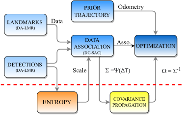
Figure 1: The complete pipeline of our self-tuning geo-referencing approach. The blue blocks indicate the standard localization architecture, and the orange block calculates the data information used to tune the data association method. Both data representation and association are previously presented in [4]. The yellow block represents the covariance propagation to associations depending on the relative transformation of the DC-SAC results.

In theory, geo-referencing could be classified in the category of localization methods with a previously built map. However, it has particularities that can differentiate it from the other localization approaches in practice. For example, it has special requirements such as a global frame referenced prior, like GNSS, or an outdoor environment that is visible from planes or satellites. Also, as an environmental requirement, the landmarks selected to perform the localization must be observable for both satellite systems and on-board sensors. Such requirements cause sparsity or aliasing problems to the landmarks that meet them.

We consider lane markings the potentially best observable landmarks for geo-referencing approaches. However, while lane markings usually offer sufficient information in lateral direction, they are often ambiguous in the direction of travel, leading to aliasing. This aliasing effect produces an unfavorable scenario where the data association suffers from many outliers. In other words, we can see an aliasing scenario equivalent to an outlier regime. Most of the works in geo-referencing usually don’t pay attention to aliasing and outliers problems because they are typically constrained to urban environments. In this work, we generalize to perform geo-referencing for both urban and rural scenarios. For that reason, we need to focus on avoiding the problem of aliasing and outliers.

For the past years, there has been a wide variety of works that aims to perform outlier mitigation in localization by using different approaches, such as convex relaxation [5] or covariance scaling [6]. Those approaches focus on robust performance of the objective function in the inference of graph-based probabilistic models. In contrast, automatic parameter tuning is another strategy to tune the back-end process depending on the low-level (the front end) data information [1]. We base our research on the last-mentioned approach. But, in our case, to provide improved data to the back-end, we self-tune the data association, that is, in the front-end.

In this paper, we present a complete geo-referencing pipeline using lane markings as landmarks. We base our system on robust performance by self-tunning capabilities to avoid the problem of aliasing and hence outliers derived from the use of lane markings. Given our delta-angle lane marking representation (DA-LMR) [4], we quantify the information of the data in terms of the curvature of the lane marking for each data association execution. Then, by using our distance-compatible sample consensus (DC-SAC) [4] data association, we can tune the search space depending on the information content of the measurements. In this way, when there is rich information like in intersections, DC-SAC can successfully search a wide space, making it robust to a bad prior. At the same time, in case of aliasing or poor information due to straight, solid markings, the data association is defaulting to a nearest neighbor search. Additionally, as DC-SAC is a pose estimation method, we adjust the covariance of the association depending on the pose results of the data association process. This kind of covariance adjustment prevents abrupt changes in the final pose.

Our work contributions can be summarized as follows:

• A complete pipeline for geo-referencing using lane markings. We use these kind of landmarks to generalize the localization for both rural and urban environments by avoiding the aliasing effect.

• Self-tuning data association. In our approach, the search space in data association depends on the data information quantified previously through our lane marking representation (DA-LMR [4]).

• Covariance adjustment that depends on the relative transformation resulting from the data association process.

The rest of the paper is organized as follows: In Section II, we review the related works in geo-referencing and localization with outlier mitigation. In Section III, we describe the proposed model for the optimization problem. Then, the main contributions, self-tuning data association, and covariance adjustment are explained in Section IV and Section V, respectively. Next, in Section VI, we present the evaluation results. Finally, Section VII exposes the main conclusions derived from this work and possible future works.

II RELATED WORK

In this section, we briefly review existing geo-referencing approaches. Additionally, we review localization approaches with outlier mitigation.

II-A Geo-referencing

As we previously mentioned, the type of landmarks selected to perform geo-referencing should be observable from both aerial images and on-board sensors. Building walls are commonly used in a wide variety of works. In [7, 8], the authors obtain information about buildings from OSM and detect walls by using LiDAR sensors. In other works [9, 10], buildings are also used as landmarks, but in this case, the authors obtain the information directly by detection in aerial geo-referenced images. In [11], the authors use semantic descriptors performed also using buildings information. In such cases, buildings landmarks carry the dependency on navigating within urban environments. In some works [12, 13, 14], the strategy of matching the vehicle’s trajectory with lanes obtained from OSM or aerial imagery is used. Such approaches are not dependent on the urban environment in theory, but in practice, the achievable accuracy using lanes is considerably lower than when using individual lane markings. This holds particularly on outer-urban roads.

Other approaches are based on learning methods [15, 16, 17], where a place is recognized from both aerial imagery and on-board sensors. Such strategies usually suffer from feature sparsity in the rural areas and depend strongly on rich-information environments, such as urban. In the method proposed in [18], the authors use reflectivity information to co-register information from LiDAR sensors and aerial imagery. As when using lane markings, this approach can suffer from aliasing, especially in rural environments, but ignores this issue.

In [3], the authors use lane markings and poles as landmarks for geo-referencing, allowing localization in rural environments. However, we consider poles hard to detect from aerial imagery, so we choose only lane markings for this work. In [3], geo-referencing is performed to achieve global consistency of maps that were created using a SLAM algorithm with on-board sensor data.

All discussed geo-referencing works either cannot achieve comparable accuracy compared to using landmarks like lane markings, suffer detection challenges and/or suffer from aliasing. In contrast, we combine easily detectable landmarks that allow highly accurate geo-referencing with a robust solution for the aliasing problem that such landmarks suffer from. An alternative to the explicit handling of aliasing issues are localization methods with outlier mitigation.

II-B Localization with outlier mitigation

The localization problem can be divided into two main components: the front end and the back end [1]. The front end involves landmarks detection, data representation, data association, etc. At the same time, the back end infers the abstracted information provided by the low-level layer (the front end). While the problem of aliasing and outliers in the data association process occurs at the front end level, it is common to prevent its consequences on the inference, i. e., at the back end layer. Traditionally, outlier mitigation in localization relied on robust M-estimators [19], such as in [20], where the authors use the Huber loss. Additionally to Huber loss, in [6], the authors use a robust function that dynamically scales the covariance to reduce the influence of measurements with significant errors. An additional experimental analysis of the covariance scaling method is available in [21]. A popular strategy to deal with outliers is the convex relaxation of the objective function in the optimization process, where [22, 5] are seminal works. Instead of mitigating the effect of the outliers, in [23, 24], the authors use convex relaxations for outliers rejection.

Previously mentioned works are focused on tuning the objective functions in the inference of graph-based probabilistic models. In contrast, other approaches aim at the problem in the whole back-end structure. For instance, in [25], the authors model ambiguous measurements using hyperedges and a multimodal mixture of Gaussian constraints. Continuous and discrete graphical models are mixed in [26] to avoid perceptual aliasing. In [27], the authors deal with a two-state implicit filter to perform outlier rejection.

Another robust performance to deal with outliers is the self-tuning strategy. Here, the front end’s data information can usually tune the objective function [28, 29] or even adjusts the graphical model [30].

Dealing with outlier mitigation in the back end is essential because the presence of outliers is expected, and the high-level layer must be ready. However, we focus our research on mitigating the outliers in the front end to pass the information as cleanly as possible to the back end. Concretely in the data association process where we perform self-tuning capabilities.

In the next section, we briefly introduce the graphical model defined for the back end of the proposed geo-referencing.

Figure 2: Example of 2D projected polylines for a set of detections $\mathcal{D}_{i}$. We mark in colors four polylines that we represent as 1D signals in Fig. 3.

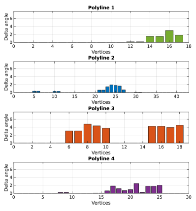
Figure 3: Example of 1D signals $\mathbf{\Delta}_{h}$ derived from polylines represented in Fig. 2 with different colors.

III GRAPH MODEL DEFINITION

We assume that we have a prior localization in world frame coordinates. Such localization could come from GNSS fusion with odometry systems or SLAM approaches, among others. We define the prior trajectory as $\hat{\mathbf{X}}=(\hat{\mathbf{x}}_{1},...,\hat{\mathbf{x}}_{N})$, where $\hat{\mathbf{x}}_{i}\doteq(\hat{\mathbf{R}}_{i},\hat{\mathbf{t}}_{i})$, $\hat{\mathbf{t}}_{i}\in\mathbb{R}^{2}$ is the translation, and $\hat{\mathbf{R}}_{i}\in SO(2)$ is the rotation matrix. We also assume that we have a word’s representation defined as a set of landmark $\mathcal{L}$. Then, for each $i$-th frame defined by $\hat{\mathbf{X}}$, we observe the landmarks of the environment using on-board sensors. We name these observations as detections $\mathcal{D}_{i}$ from now on. Using $\mathcal{L}$ and $\mathcal{D}_{i}$, we perform a data association process, where its result is defined by $\mathbf{A}_{i}=((\mathbf{d}_{i_{1}},\mathbf{l}_{i_{1}}),...,(\mathbf{d}_{i_{M}},\mathbf{l}_{i_{M}}))$. Given these associations, if we express as $\mathbf{X}$ the pose estimated in the optimization process, we can define the residuals between landmarks and detections as follows:

$$e^{\mathbf{A}}(\mathbf{X})=\sum_{i=1}^{N}\sum_{k=1}^{M}\left\lVert\left(\mathbf{R}_{i}\mathbf{d}_{i_{k}}+\mathbf{t}_{i}\right)-\mathbf{l}_{i_{k}}\right\rVert^{2}_{\Sigma_{i_{k}}}$$ (1)

Where $\Sigma_{i_{k}}$ is the covariance matrix of each detection $\mathbf{d}_{i_{k}}$. The covariance is transformed into an information matrix $\Omega_{i_{k}}=\Sigma^{-1}_{i_{k}}$ that weighs the residuals as $e^{\mathsf{T}}_{i_{k}}\Omega_{i_{k}}e_{i_{k}}$.

Additionally, given the relative transformations from consecutive frames $i$ and $j$ from the prior trajectory $\hat{\mathbf{X}}$ and the estimated $\mathbf{X}$, we can define the odometry residuals as follows:

$$e^{\hat{\mathbf{X}}}(\mathbf{X})=\sum_{i,j}^{N}\left\lVert\hat{\mathbf{R}}^{\mathsf{T}}_{i}\left(\hat{\mathbf{t}}_{j}-\hat{\mathbf{t}}_{i}\right)-\mathbf{t}_{ij}\right\rVert^{2}+\left\lVert\hat{\mathbf{R}}^{\mathsf{T}}_{i}\hat{\mathbf{R}}_{j}-\mathbf{R}_{ij}\right\rVert^{2}_{\Lambda_{i}}$$ (2)

Where $\Lambda_{i}$ is the covariance matrix of each relative transform. Hence, given the residuals, graph-based localization aims to estimate the trajectory $\mathbf{X}^{*}$ that minimizes the error function:

$$\mathbf{X}^{*}=\operatornamewithlimits{arg\ min}_{\mathbf{X}}\left(e^{\mathbf{A}}(\mathbf{X})+e^{\hat{\mathbf{X}}}(\mathbf{X})\right)$$ (3)

This is an optimization problem, and we use a Gauss-Newton Non-linear Least Square (NLS) approach to solve it.

IV SELF-TUNING DATA ASSOCIATION

We consider lane marking the best visible landmarks for aerial imagery and on-board sensors for urban and road scenarios. Then, previously defined $\mathcal{L}$ and $\mathcal{D}_{i}$ contains these kinds of features. The problem is that given the aliasing risk in the straight roads for lane markings, the associations $\mathbf{A}_{i}$ usually have outliers.

In Section IV-A, we analyze the detections to quantify how straight the road is by using our DA-LMR lane marking representation [4]. This is directly related to the information theoretical entropy of the detections. Then, to mitigate outliers, in Section IV-B, we tune the search area of our DC-SAC data association [4] depending on the local pseudo-entropy of the road.

IV-A Pseudo-entropy quantification by DA-LMR

We can think of lane marking as polylines, while our DA-LMR [4] defines each one as a set of 3D points $\mathbf{P}^{3D}=(\mathbf{p}^{3D}_{0},\mathbf{p}^{3D}_{1},...,\mathbf{p}^{3D}_{n})$ where

$$\mathbf{p}^{3D}_{l}=(x_{l},y_{l},\Delta\alpha_{l}w).$$ (4)

The third dimension of that representation encodes the differential angle $\Delta\alpha_{l}$ between adjacent segments in polyline weighed with a configurable parameter $w$. We show in Fig. 2 an example of 2D projected polylines for a set of detections $\mathcal{D}_{i}$.

To measure how straight the road that the data represents is, for each $h$-th polyline, we extract the delta angle from DA-LMR and describe it as a 1D signal $\mathbf{\Delta}_{h}=(\Delta\alpha_{h_{1}},...,\Delta\alpha_{h_{n}})$. In Fig. 3, we depicted the 1D signals $\mathbf{\Delta}_{h}$ from polylines represented in Fig. 2. Then with this representation, we can calculate the information as follows:

$$S=-\sum_{h=1}^{m}\sum_{l=1}^{n}\Delta\alpha_{h_{l}}\log(\Delta\alpha_{h_{l}}+1)$$ (5)

The index $h$ refers to entire polylines, while $l$ indexes each element in the polyline. $S$ is not a by-definition entropy as $\mathbf{\Delta}_{h}$ is not a probabilistic distribution. However, regularizing the logarithm by $+1$ term, the behavior is similar, and we can consider $S$ as a pseudo-entropy calculation. But, to simplify the terminology, subsequently, we think of $S$ as entropy.

To understand this quantification, we can consider an example of detections on a straight road. In that case, the lane markings are linear, and $\Delta\alpha_{h_{l}}$ values are close to $0$. Hence, the measure of $S$ is also close to $0$. Then we can consider this case as low informative for the data association process. In contrast, the example depicted in Fig. 2 contains polylines with an amount of information concentrated in corners. Then, the value of $S$ can achieve high negative values. Hence, we can consider this as an example of highly informative detections.

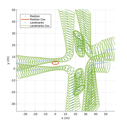
Figure 4: Covariance propagation in a set $\mathcal{D}_{i}$, where the red ellipse indicates the data association covariance $\Sigma_{i}$ and the green ellipses depict the detections covariances propagated $\Sigma_{i_{k}}$.

IV-B Data association by DC-SAC

The DC-SAC data association method [4] randomly samples a pair of points in $\mathcal{D}_{i}$ and a couple of distance-compatible points in $\mathcal{L}$. Given the samples, we obtain the transform $\Delta\mathbf{T}\in SE(2)$ that minimizes the error between the pairs by solving the Procrustes problem. We repeat this process generating a hypothesis space $\mathcal{H}$. The final association comes from the $\Delta\mathbf{T}^{*}\in\mathcal{H}$ that achieves the minimum error from the inliers between $\mathcal{D}_{i}(\Delta\mathbf{T}^{*})$ and $\mathcal{L}$.

As explained in [4], $\mathcal{H}$ could be reduced by limiting the sample area size defined by configurable parameters $\Phi=(x_{max},y_{max},\theta_{max})$. That means we can discard the $\Delta\mathbf{T}\in\mathcal{H}$ that fall out of the area defined by $\Phi$. We observed that DC-SAC, with proper $\Phi$ configuration, produces excellent results with a highly informative set $\mathcal{D}_{i}$, as the one shown in Fig. 2. However, in straight roads, it suffers, like others, from an aliasing effect that produces outliers.

It is worth noting that when $\Phi\xrightarrow{}0$, the space $\mathcal{H}$ only contains a default transform $\Delta\mathbf{T}\triangleq 0$. Hence, the associations come from the inliers between $\mathcal{D}_{i}$ and $\mathcal{L}$. This behavior is equivalent to the classical Nearest Neighbour (NN) data association. For straight markings, NN can mitigate that aliasing effect as good as possible given the odometry’s information. In contrast, NN does not exploit highly informative environments.

Then, given DC-SAC and NN’s complementary behavior, we can self-tune the parameters $\Phi_{i}$ dynamically for each $\mathcal{D}_{i}$ by using the entropy information as follows:

$$\Phi^{tuned}_{i}=\left\{\begin{array}[]{ll}\Phi,&S_{i}\leq S_{min}\\ \Phi\left|\frac{S_{i}}{S_{min}}\right|,&S_{i}>S_{min}\\ \end{array}\right.$$ (6)

$S_{min}$ is a configurable parameter that saturates the limit of the minimum value of entropy, thus controlling the ramp for the tuning. We can see in (6) that when $S\xrightarrow{}0$ (e.g. straight road), the behavior is close to NN, and when $S\xrightarrow{}S_{min}$ (e.g. intersection), the behavior comes to DC-SAC in its maximum sample area size configuration. And in the middle point, we have linear changes. This area size self-tuning capability mitigates the aliasing effect dramatically and, hence, the outlier risk, as we demonstrate experimentally in Section VI.

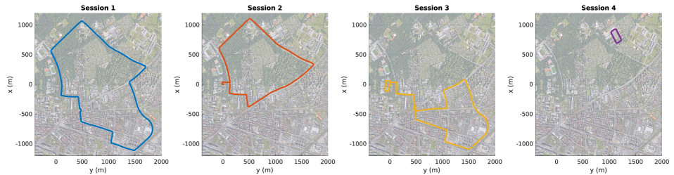
Figure 5: The four closed trajectories for evaluation, driving through the city of Karlsruhe (Germany) and its outer roads. In Table II, we show more details about these trajectories.

V DYNAMIC COVARIANCE ADJUSTMENT

In addition to the already explained self-tuned data association, we implemented another layer of robustness by dynamic covariance adjustment. For each data association process, we estimate a covariance matrix depending on the result of DC-SAC (Section V-A). Afterward, we propagate that covariance to detections by first-order transformation (Section V-B), and we use the inverse as an information matrix in the optimization process.

V-A Data association variance

We defined in Section III the prior trajectory as $\hat{\mathbf{X}}=(\hat{\mathbf{x}}_{1},...,\hat{\mathbf{x}}_{N})$, and in the same way, we can define the estimated trajectory as $\mathbf{X}=(\mathbf{x}_{1},...,\mathbf{x}_{N})$. However, in the data association stage, before pose estimation $\mathbf{X}$ at $i$-th sample time, we can pre-estimate the pose by using $\mathbf{x}_{i-1}$ and integrating the last differential of the prior $\Delta\hat{\mathbf{x}}_{i-1,i}$. Then, we can express the pre-estimation as $\bar{\mathbf{x}}_{i}=\mathbf{x}_{i-1}\Delta\hat{\mathbf{x}}_{i-1,i}$.

DC-SAC data association method is pose-based, which means that apart from the associations $\mathbf{A}_{i}$, the result also contains the relative transform $\Delta\mathbf{T}^{*}_{i}\in\mathcal{H}_{i}$ that produces $\mathbf{A}_{i}$. The transform $\Delta\mathbf{T}^{*}_{i}$ is relative to previously explained $\bar{\mathbf{x}}_{i}$.

If we think in a hypothetical ideal case of localization without errors, the relative transforms $\bar{\mathbf{T}}=(\Delta\mathbf{T}_{1},...,\Delta\mathbf{T}_{N})$ should have $\Delta\mathbf{T}_{i}\triangleq 0$ in all cases. Hence, in the real case, we can assume that when the evolution of $\bar{\mathbf{T}}$ is stable, the data association is reliable. In contrast, when $\bar{\mathbf{T}}$ has a strong variance, the data association results are unreliable. In theory, the stable behavior of $\Delta\mathbf{T}_{i}$ can also come from the localization to a local minimum. However, we had not inconvenience at this point in the experiments because we have the main self-tuning layer described in Section IV. In this way, the localization can be corrected in the areas of high informative data avoiding possible local minimums.

Under the previously-mentioned assumption, we perform the covariance matrix as:

$$\Sigma_{i}=\Psi(\Delta\mathbf{T}_{i-W},...,\Delta\mathbf{T}_{i})$$ (7)

Where $\Psi$ is a function that calculates the variance, and $W$ is a configurable parameter that defines a window to select the last data association results.

V-B Covariance propagation

The covariance matrix $\Sigma_{i}$ is expressed in the sensor coordinate frame. To make it suitable for constraints (1), we use first-order transformation to propagate the covariance to detections [31], obtaining $\Sigma_{i_{k}}$.

We have estimated pose $\mathbf{x}_{i}\doteq(\mathbf{R}_{i},\mathbf{t}_{i})$, where $\mathbf{t}_{i}=(x_{i},y_{i})$. Then, if we express detections as $\mathbf{d}_{i_{k}}=(x_{i_{k}}^{d},y_{i_{k}}^{d})$ in the sensor coordinate frame, we can transform detections to estimation coordinate frame as:

$$f_{i_{k}}^{x}=x_{i_{k}}^{d}\cos\theta_{i}-y_{i_{k}}^{d}\sin\theta_{i}+x_{i}$$ (8)

$$f_{i_{k}}^{y}=x_{i_{k}}^{d}\sin\theta_{i}+y_{i_{k}}^{d}\cos\theta_{i}+y_{i}$$ (9)

If we compute the first-order derivative, we obtain the Jacobian:

$$J_{i_{k}}=\begin{bmatrix}\frac{\partial f_{i_{k}}^{x}}{x_{i}}&\frac{\partial f_{i_{k}}^{x}}{y_{i}}&\frac{\partial f_{i_{k}}^{x}}{\theta_{i}}\\ \frac{\partial f_{i_{k}}^{y}}{x_{i}}&\frac{\partial f_{i_{k}}^{y}}{y_{i}}&\frac{\partial f_{i_{k}}^{y}}{\theta_{i}}\end{bmatrix}=\begin{bmatrix}1&0&-x_{i_{k}}^{d}\sin\theta-y_{i_{k}}^{d}\cos\theta\\ 0&1&x_{i_{k}}^{d}\cos\theta+y_{i_{k}}^{d}\sin\theta\end{bmatrix}$$ (10)

Given the Jacobian, we can propagate the covariance to detections as follows:

$$\Sigma_{i_{k}}=J_{i_{k}}\Sigma_{i}J_{i_{k}}^{\mathsf{T}}$$ (11)

In Fig. 4, we show an example of covariance propagation, where the red ellipse indicates the data association covariance $\Sigma_{i}$ and the green ellipses depict the detections covariances propagated $\Sigma_{i_{k}}$.

TABLE I: Trajectory evaluation by Absolute Trajectory Error (ATE) in meters.

			DC-SAC	Self-Tuning	Self-Tuning	Covariance	Convex
Session	Prior	NN (static)	(static)	- Cov. Adj.	+ Cov. Adj.	Scaling [6]	Relaxation [5]
1	2.61	4.14	11.23	0.14	0.07	0.38	0.24
2	3.36	4.87	10.29	0.67	0.09	0.36	0.21
3	3.35	1.67	8.54	0.25	0.06	0.29	0.27
4	2.68	0.74	2.21	0.09	0.06	0.16	0.14

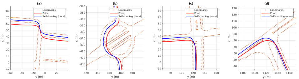
Figure 6: Comparison between the prior trajectories (red lines) and the geo-referenced ones estimated using the proposed self-tuning method (blue lines). The points are the landmarks $\mathcal{L}$ inside a window.

VI EVALUATION

In this section, we show the results of our evaluation. First (Section VI-A), we comment on the experimental setup. Next (Section VI-B), we assessed the trajectory compared with different configurations and state-of-the-art methods. And finally (Section VI-C), we focus on the evaluation of outlier mitigation.

VI-A Experimental setup

The evaluation consists of four closed trajectories driven through the city of Karlsruhe (Germany) and its outer roads (Fig. 5 and Table II). The four sessions are initially referenced with low-cost GNSS measurements using the approach proposed in [32], and the results are used as a prior trajectory. Each prior pose has its corresponding lane markings detections $\mathcal{D}_{i}$. To perform that process, we used the experimental vehicle BerthaOne [33]. The car comprises four Velodyne VLP16 LiDARs mounted flat on the roof, three BlackFly PGE-50S5M cameras behind the front and rear windshield, and a Ublox C94-M8P GNSS receiver. To test the proposed geo-referencing approach, we use a hand-made map built from geo-referenced aerial images around the area where we completed the trajectories. This map consists of a set of lane markings landmarks $\mathcal{L}$.

TABLE II: Sessions characteristics description.

Session	Scan Number	Length (km)	Environment
1	5085	7.09	Urban + Rural
2	4172	5.49	Urban + Rural
3	5105	6.63	Urban
4	598	0.73	Rural

VI-B Trajectory evaluation

Using $\mathcal{L}$ as a reference, we built a hand-made ground truth consisting of an artificial trajectory (for each session) that contains a set of positions drawn by hand following the center of transited lanes. Each ground truth position is marked for each $i$-th sample in the prior trajectory. Given this ground truth as a reference, we evaluate the prior trajectory through the Absolute Trajectory Error (ATE) metric [34], and compare it with different configurations of our approach: NN (ours with $\Phi=($0\text{\,}\mathrm{m}$,$0\text{\,}\mathrm{m}$,$0\text{\,}\mathrm{rad}$)$), DC-SAC (ours with $\Phi=($5\text{\,}\mathrm{m}$,$5\text{\,}\mathrm{m}$,$0.2\text{\,}\mathrm{rad}$)$), Self-Tuning -Cov. Adj. (ours without covariance adjustment), and Self-Tuning +Cov. Adj. (our complete approach). Additionally, we compare it with two state-of-the-art (SOTA) methods in outlier mitigation: Covariance Scaling [6] and Convex Relaxation [5].

TABLE III: Outlier evaluation by Relative Pose Error (RPE) in translation and rotation.

			DC-SAC	Self-Tuning	Self-Tuning	Covariance	Convex
Session	RPE	NN (static)	(static)	- Cov. Adj.	+ Cov. Adj.	Scaling [6]	Relaxation [5]
1	trans. ($m$)	0.04	9.34	0.04	0.04	0.23	0.14
	rot. ($\deg$)	0.07	0.14	0.06	0.06	0.08	0.07
2	trans. ($m$)	0.04	10.00	0.06	0.06	0.25	0.13
	rot. ($\deg$)	0.07	0.13	0.12	0.12	0.16	0.14
3	trans. ($m$)	0.04	9.88	0.07	0.06	0.28	0.16
	rot. ($\deg$)	0.08	0.17	0.11	0.11	0.15	0.12
4	trans. ($m$)	0.04	3.38	0.06	0.06	0.18	0.16
	rot. ($\deg$)	0.08	0.13	0.11	0.09	0.14	0.10

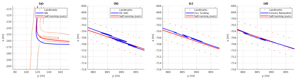
Figure 7: Comparison between the estimated trajectories using the proposed self-tuning method (red lines) and the compared configurations and SOTA methods (blue lines): (a) NN, (b) DC-SAC, (c) covariance scaling, and (d) convex relaxation.

Table I shows the results in ATE metric between trajectories estimated from different configurations and methods mentioned and ground truth. Due to ground truth only containing positions, we only calculate ATE for translation.

Due to its challenging aliasing problems, we can see the most significant error in the DC-SAC configuration. In the NN configuration, we do not have the aliasing problem, but there is a scaling problem that has the configuration unreliable (we will depict it in the next section Fig. 7 (a)). The compared SOTA methods mitigate the aliasing effect but not sufficiently. We can see that we achieve the best results with our self-tuning approach, especially with the combination using the covariance adjustment.

In Fig. 6, we show in blue a qualitative examples of trajectories estimated though the proposed self-tuning geo-referenceing. In all cases, the course is located in the center of the lane. In contrast, we show in red the prior trajectories that always are out of the lanes.

VI-C Outlier mitigation evaluation

The prior used for the evaluation is globally inconsistent but locally little noisy. That means the differential information has no considerable errors. Hence, we can use that relative prior information as a reference to evaluate the effects of outliers by using the alternative Relative Pose Error (RPE) metric [34].

In Table III, we show RPE results to compare the configurations and SOTA methods named in the previous section. In this case, we can see that the error in the NN configuration is similar to the complete self-tuning approach. This is because, as previously-mentioned, the NN has no aliasing problems. However, in Fig. 7 (a), we depict the main problem of that configuration, where the red line indicates the trajectory estimated with our complete approach, and the blue line indicates the NN configuration path with the flaw of scaling problems that produces localization out of the lane.

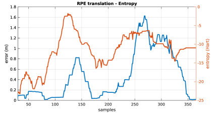
Figure 8: The individual pose RPE evolution in an arbitrary trajectory window in contrast with the entropy for the same poses.

We can see in Table III that the DC-SAC configuration suffers hardly from aliasing problems that produce a considerable number of outliers. In Fig. 7 (b), we depict the aliasing effect in a straight road compared to our self-tuning approach. As shown in Table III and Fig. 7, the SOTA methods of covariance scaling and convex relaxation can mitigate the effect of outliers but don’t achieve the results of our self-tuning approach for this scenario. We can observe that angle RPE is commonly close to 0, which indicates that significant errors are always produced in the front direction due to aliasing problems.

Finally, to demonstrate our assumption of the relationship between the data entropy and the outliers, we show the individual pose RPE evolution in an arbitrary trajectory window for non-tuning DC-SAC configuration in contrast with the entropy for the same poses. We can see in Fig. 8 that exists a direct correlation.

VII CONCLUSIONS

This paper presented a complete geo-referencing pipeline using lane markings as landmarks. To address the outliers problems derived from aliasing, we performed a robust implementation providing self-tuning capabilities to our DC-SAC data association by adapting the search area depending on the entropy in the measurements represented by our lane marking representation (DA-LMR). Additionally, to smooth the final result, we adjusted the information matrix for the associated data as a function of the relative transform produced by the DC-SAC. We demonstrated considerable outlier mitigation, especially on straight roads, compared with other state-of-the-art robust implementations by the experiments performed in urban and outer-urban scenarios, both of which contained areas with high ambiguity for data association.

In future work, we plan to extend our approach to new kinds of landmarks, such as walls or even complete buildings, and an automatic landmarks extraction from the aerial imagery.

References

- [1] C. Cadena, L. Carlone, H. Carrillo, Y. Latif, D. Scaramuzza, J. Neira, I. Reid, and J. J. Leonard, “Past, present, and future of simultaneous localization and mapping: Toward the robust-perception age,” IEEE Transactions on robotics, vol. 32, no. 6, pp. 1309–1332, 2016.
- [2] J.-H. Pauls, K. Petek, F. Poggenhans, and C. Stiller, “Monocular localization in hd maps by combining semantic segmentation and distance transform,” in 2020 IEEE/RSJ International Conference on Intelligent Robots and Systems (IROS). IEEE, 2020, pp. 4595–4601.
- [3] H. Hu, M. Sons, and C. Stiller, “Accurate global trajectory alignment using poles and road markings,” in 2019 IEEE Intelligent Vehicles Symposium (IV). IEEE, 2019, pp. 1186–1191.
- [4] M. Á. Muñoz-Bañón, J.-H. Pauls, H. Hu, and C. Stiller, “Da-lmr: A robust lane marking representation for data association,” in 2022 International Conference on Robotics and Automation (ICRA). IEEE, 2022, pp. 2193–2199.
- [5] L. Carlone and G. C. Calafiore, “Convex relaxations for pose graph optimization with outliers,” IEEE Robotics and Automation Letters, vol. 3, no. 2, pp. 1160–1167, 2018.
- [6] P. Agarwal, G. D. Tipaldi, L. Spinello, C. Stachniss, and W. Burgard, “Robust map optimization using dynamic covariance scaling,” in 2013 IEEE International Conference on Robotics and Automation. Ieee, 2013, pp. 62–69.
- [7] Y. Cho, G. Kim, S. Lee, and J.-H. Ryu, “Openstreetmap-based lidar global localization in urban environment without a prior lidar map,” IEEE Robotics and Automation Letters, vol. 7, no. 2, pp. 4999–5006, 2022.
- [8] G. Floros, B. Van Der Zander, and B. Leibe, “Openstreetslam: Global vehicle localization using openstreetmaps,” in 2013 IEEE International Conference on Robotics and Automation. IEEE, 2013, pp. 1054–1059.
- [9] J. Kim and J. Kim, “Fusing lidar data and aerial imagery with perspective correction for precise localization in urban canyons,” in 2019 IEEE/RSJ International Conference on Intelligent Robots and Systems (IROS). IEEE, 2019, pp. 5298–5303.
- [10] H. Roh, J. Jeong, and A. Kim, “Aerial image based heading correction for large scale slam in an urban canyon,” IEEE Robotics and Automation Letters, vol. 2, no. 4, pp. 2232–2239, 2017.
- [11] F. Yan, O. Vysotska, and C. Stachniss, “Global localization on openstreetmap using 4-bit semantic descriptors,” in 2019 European Conference on Mobile Robots (ECMR). IEEE, 2019, pp. 1–7.
- [12] I. P. Alonso, D. F. F. Llorca, M. Gavilan, S. Á. Á. Pardo, M. Á. García-Garrido, L. Vlacic, and M. Á. Sotelo, “Accurate global localization using visual odometry and digital maps on urban environments,” IEEE Transactions on Intelligent Transportation Systems, vol. 13, no. 4, pp. 1535–1545, 2012.
- [13] M. M. Atia and S. L. Waslander, “Map-aided adaptive gnss/imu sensor fusion scheme for robust urban navigation,” Measurement, vol. 131, pp. 615–627, 2019.
- [14] B. Suger and W. Burgard, “Global outer-urban navigation with openstreetmap,” in 2017 IEEE International Conference on Robotics and Automation (ICRA). IEEE, 2017, pp. 1417–1422.
- [15] T. Y. Tang, D. De Martini, D. Barnes, and P. Newman, “Rsl-net: Localising in satellite images from a radar on the ground,” IEEE Robotics and Automation Letters, vol. 5, no. 2, pp. 1087–1094, 2020.
- [16] H. Hu, J. Zhu, S. Wirges, and M. Lauer, “Localization in aerial imagery with grid maps using locgan,” in 2019 IEEE Intelligent Transportation Systems Conference (ITSC). IEEE, 2019, pp. 2860–2865.
- [17] M. Fu, M. Zhu, Y. Yang, W. Song, and M. Wang, “Lidar-based vehicle localization on the satellite image via a neural network,” Robotics and Autonomous Systems, vol. 129, p. 103519, 2020.
- [18] A. Vora, S. Agarwal, G. Pandey, and J. McBride, “Aerial imagery based lidar localization for autonomous vehicles,” arXiv preprint arXiv:2003.11192, 2020.
- [19] P. J. Huber, Robust statistical procedures. SIAM, 1996.
- [20] M. Kaess, H. Johannsson, R. Roberts, V. Ila, J. J. Leonard, and F. Dellaert, “isam2: Incremental smoothing and mapping using the bayes tree,” The International Journal of Robotics Research, vol. 31, no. 2, pp. 216–235, 2012.
- [21] P. Agarwal, G. Grisetti, G. D. Tipaldi, L. Spinello, W. Burgard, and C. Stachniss, “Experimental analysis of dynamic covariance scaling for robust map optimization under bad initial estimates,” in 2014 IEEE International Conference on Robotics and Automation (ICRA). IEEE, 2014, pp. 3626–3631.
- [22] L. Carlone, A. Censi, and F. Dellaert, “Selecting good measurements via l1 relaxation: A convex approach for robust estimation over graphs,” in 2014 IEEE/RSJ International Conference on Intelligent Robots and Systems. IEEE, 2014, pp. 2667–2674.
- [23] H. Yang, P. Antonante, V. Tzoumas, and L. Carlone, “Graduated non-convexity for robust spatial perception: From non-minimal solvers to global outlier rejection,” IEEE Robotics and Automation Letters, vol. 5, no. 2, pp. 1127–1134, 2020.
- [24] J. Shi, H. Yang, and L. Carlone, “Robin: a graph-theoretic approach to reject outliers in robust estimation using invariants,” in 2021 IEEE International Conference on Robotics and Automation (ICRA). IEEE, 2021, pp. 13 820–13 827.
- [25] M. Pfingsthorn and A. Birk, “Generalized graph slam: Solving local and global ambiguities through multimodal and hyperedge constraints,” The International Journal of Robotics Research, vol. 35, no. 6, pp. 601–630, 2016.
- [26] P.-Y. Lajoie, S. Hu, G. Beltrame, and L. Carlone, “Modeling perceptual aliasing in slam via discrete–continuous graphical models,” IEEE Robotics and Automation Letters, vol. 4, no. 2, pp. 1232–1239, 2019.
- [27] M. Bloesch, M. Burri, H. Sommer, R. Siegwart, and M. Hutter, “The two-state implicit filter recursive estimation for mobile robots,” IEEE Robotics and Automation Letters, vol. 3, no. 1, pp. 573–580, 2017.
- [28] G. Agamennoni, P. Furgale, and R. Siegwart, “Self-tuning m-estimators,” in 2015 IEEE International Conference on Robotics and Automation (ICRA). IEEE, 2015, pp. 4628–4635.
- [29] E. R. Santos, M. A. Vieira, and G. S. Sukhatme, “Mobile robot localization under non-gaussian noise using correntropy similarity metric,” in 2020 IEEE/RSJ International Conference on Intelligent Robots and Systems (IROS). IEEE, 2020, pp. 8534–8539.
- [30] G. Soldi, F. Meyer, P. Braca, and F. Hlawatsch, “Self-tuning algorithms for multisensor-multitarget tracking using belief propagation,” IEEE Transactions on Signal Processing, vol. 67, no. 15, pp. 3922–3937, 2019.
- [31] P. Roysdon and J. Farrell, “Technical note: Ins noise propagation,” Technical report, October, Tech. Rep., 2018.
- [32] M. Sons and C. Stiller, “Efficient multi-drive map optimization towards life-long localization using surround view,” in 2018 21st International Conference on Intelligent Transportation Systems (ITSC). IEEE, 2018, pp. 2671–2677.
- [33] Ö. Ş. Taş, N. O. Salscheider, F. Poggenhans, S. Wirges, C. Bandera, M. R. Zofka, T. Strauss, J. M. Zöllner, and C. Stiller, “Making bertha cooperate–team annieway’s entry to the 2016 grand cooperative driving challenge,” IEEE Transactions on Intelligent Transportation Systems, vol. 19, no. 4, pp. 1262–1276, 2017.
- [34] D. Prokhorov, D. Zhukov, O. Barinova, K. Anton, and A. Vorontsova, “Measuring robustness of visual slam,” in 2019 16th International Conference on Machine Vision Applications (MVA). IEEE, 2019, pp. 1–6.