Directional Josephson traveling-wave parametric amplifier via non-Hermitian topology

Abstract

Low-noise microwave amplifiers are crucial for detecting weak signals in quantum technologies and radio astronomy. Building an ideal device is challenging as it must amplify a broad range of frequencies while adding minimal noise. The amplification must also be directional so that it favors the observer’s direction while protecting the source from its environment. Here, we introduce a fundamentally new type of superconducting Josephson traveling-wave parametric amplifier that fulfills all these requirements by exploiting non-Hermitian topological effects and time-reversal symmetry breaking via the phase of the four-wave-mixing pump. In the topological amplification phase, the device acquires an unprecedented performance such as a gain growing exponentially with system size and largely surpassing 20 dB, exponential suppression of back-wards noise below -30 dB, a bandwidth of GHz, and topological protection against disorder. This opens the door for integrating near-ideal and compact pre-amplifiers on the same chip as quantum processors.

I Introduction

Low-noise amplification enables high-sensitivity applications ranging from astronomic instrumentation [1] to nano-mechanical sensing [2]. In superconducting quantum technology [3, 4], in particular, microwave signals carrying quantum information are so weak that near quantum-limited amplification is indispensable to detect them in a single-shot measurement [5, 6, 7, 8]. In this respect, the most advanced amplifiers currently available are Josephson traveling-wave parametric amplifiers (JTWPAs) which are built of a carefully engineered array of Josephson junctions (JJs) [9, 10, 11, 12]. Activating the Kerr non-linearities via four-wave-mixing [13, 14], these devices have demonstrated a great amplification performance with gains above 20 dB, near quantum-limited noise, and a large bandwidth in the GHz range [15]. An important drawback is that JTWPAs are not truly directional, meaning that parasitic signals and vacuum fluctuations can be back-amplified and contaminate the quantum source. In practice, this is avoided by equipping the JTWPAs with isolators, but these are bulky and lossy external elements that limit the efficiency and scalability of superconducting quantum devices.

Directional amplification has only been realized on few-mode non-reciprocal devices [16, 17, 18, 19, 20, 21], which are fundamentally narrowband. Broadband amplification is crucial towards implementing large-scale quantum information processors, where multiple signals need to be multiplexed and simultaneously detected [22]. Therefore, unifying the broadband properties of JTWPAs with the compactness of a directional amplifier with built-in backwards isolation is one of the holy grails in the field [15].

In this work, we combine concepts of topological photonics [23, 24, 25, 26, 27] and Josephson parametric amplification [13, 14, 15] to devise a radically new type of JTWPA that is intrinsically directional/non-reciprocal, while retaining all excellent amplifying properties of conventional designs such as gain, noise, and bandwidth. The key to build a topological JTWPA is to perform the four-wave-mixing process via a global pump on all sites of a JJ array, which we achieve indirectly via an auxiliary resonator array [see Fig. 1(a,b)]. Controlling the phase dependence of this pump $\sim\phi j$ allows us to implement perfect phase matching along the JJ array and, most remarkably, to induce a synthetic gauge field that breaks time-reversal symmetry (TRS) [28], without requiring dispersion engineering [9, 10, 11], Floquet engineering [29, 30, 31] or external magnetic fields. The combination of this gauge field, non-local parametric pump induced by Kerr non-linearities, and homogeneous local dissipation, allows us to stabilize a steady-state with topological amplifying properties. In this driven-dissipative phase, the system exhibits directional and near-quantum-limited amplification of microwave signals with a gain that grows exponentially with the array size while keeping a large bandwidth on the order of the effective hopping. The directionality is manifested by an exponential suppression of all backwards added noise and signals propagating towards the source. Moreover, the device has topological protection against disorder in all system parameters and, in particular, to imperfections inherent in the fabrication of JJs [32].

Beyond proposing the design of this novel topological JTWPA, we also characterize its performance at various operation points, and demonstrate the feasibility to implement it with current superconducting circuit technology [33, 34, 35]. We predict that a device with $N\lesssim 30$ sites can provide near quantum-limited amplification over a bandwidth of GHz with more than 20 dB of gain and -30 dB of backwards attenuation. This is two orders of magnitude larger in bandwidth and directionality than previous non-reciprocal amplifiers [16, 17, 18, 19, 20, 21]. We also show that a topological JTWPA with just $N=4$ sites can be operated as an ultra low-noise directional amplifier with just 0.06 noise photons above the quantum limit. Our work thus provides a promising route towards the scalable integration of near-ideal pre-amplifiers and quantum processors on the same on-chip, avoiding the use of external isolators.

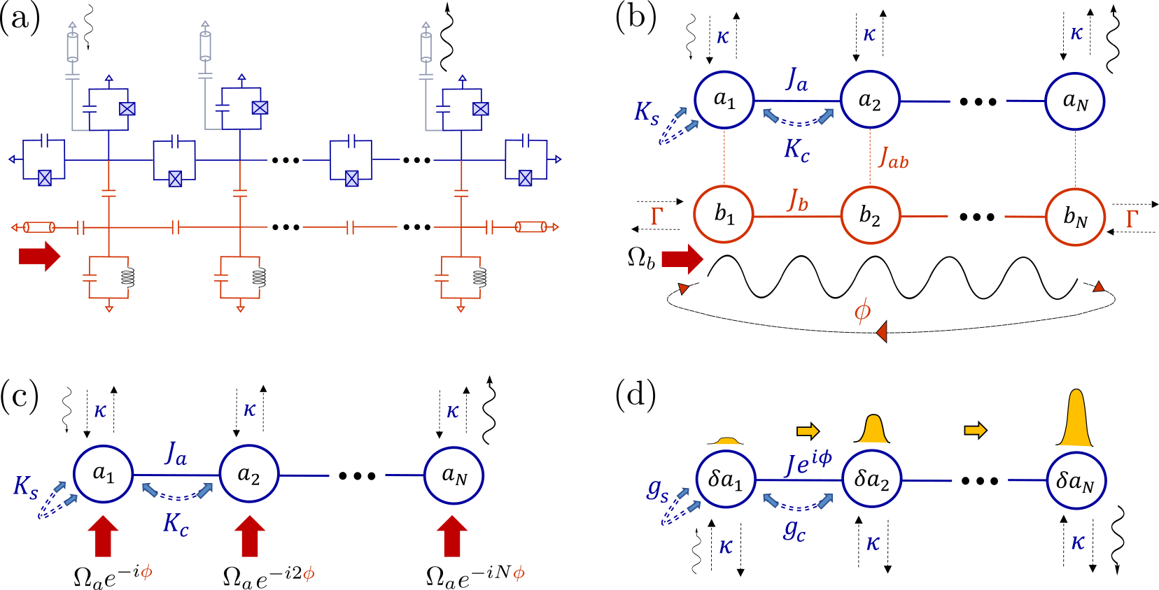
Figure 1: Realization of a topological Josephson traveling-wave parametric amplifier (JTWPA). (a) Superconducting circuit scheme composed of a JJ array (blue), where each site $j=1,\dots,N$ is coupled to a $50\Omega$ input/output line (grey), and to an auxiliary array of linear superconducting resonators (red). All couplings are capacitive and linear except for the JJ array, where Josephson junctions mediate nonlinear Kerr interactions. Signals are sent/retrieved via input/output ports of the JJ array (black curvy arrows), while the strong pump for four-wave mixing is sent through the auxiliary array (red arrow). (b) Quantum optics model implemented by the superconducting circuit in (a). The JJ array implements an array of anharmonic modes $a_{j}$ with self- and cross-Kerr nonlinear couplings $K_{s}$ and $K_{c}$, as well as linear hopping $J_{a}$. The auxiliary array modes $b_{j}$ are linearly coupled via intra- and inter-array couplings $J_{b}$ and $J_{ab}$, respectively. Transmission lines provide local decays $\kappa$ to each $a_{j}$ mode, and a $\Gamma=2J_{b}$ decay to auxiliary modes at the boundaries, $b_{1}$ and $b_{N}$. The mode $b_{1}$ is coherently driven with strength $\Omega_{b}$ to generate a classical right-moving running-wave of phase $\phi=\pi/2$. (c) The net effect of the auxiliary array is to distribute a collective pump $\Omega_{a}=(J_{ab}/2J_{b})\Omega_{b}$ on all sites of the JJ array. This is used to perform four-wave-mixing and break TRS via its spatially varying phase $\sim j\phi$. (d) Topological amplifier model appearing in the linearized dynamics of the quantum fluctuations $\delta a_{j}$ of the JJ array. The combination of complex hopping $Je^{i\phi}$, local decay $\kappa$, and parametric local and non-local pumping terms $g_{s}$ and $g_{c}$, leads the system to a topological steady-state phase, where external signals entering at site $j=1$ are directionally amplified and accumulate at the right boundary $j=N$.

II Topological Josephson traveling wave parametric amplifier

Fig. 1(a,b) displays the superconducting circuit scheme and the associated quantum optics model to realize a topological JTWPA. It consists of a homogeneous JJ array of $N$ sites (blue) that is coupled to local input/output ports on each site (grey), as well as to an auxiliary array of linear resonators (red). The backbone of the setup is the JJ array, where on-site capacitors and JJs give rise to localized microwave modes $a_{j}$ with large on-site frequencies $\omega_{a}\sim\mathrm{GHz}$ and weak self-Kerr anharmonicities $K_{s}\lesssim\mathrm{MHz}$. These modes, which behave similarly to weakly anharmonic Transmons [3, 4], are coupled via additional inter-site capacitors and JJs leading to linear hoppings $J_{a}$ and non-linear cross-Kerr interactions $K_{c}$ between neighboring sites [cf. Fig. 1(a)-(b), blue]. The dynamics of the JJ array is then governed by the lattice Hamiltonian,

$$H_{\rm JJA}={} \omega_{a}\sum_{j}a_{j}^{\dagger}a_{j}-\frac{K_{s}}{2}\sum_{j}a_{j}^{\dagger}a_{j}^{\dagger}a_{j}a_{j}$$ (1)

$$+{} J_{a}\sum_{j}(a_{j+1}^{\dagger}a_{j}+h.c.)-K_{c}\sum_{j}a_{j+1}^{\dagger}a_{j+1}a_{j}^{\dagger}a_{j}.$$

Arrays of JJs have been extensively studied for implementing conventional JTWPAs, but they typically do not include on-site JJs and therefore behave like transmission lines with non-linear dispersion relation [9, 11, 36, 10, 12]. This is in stark contrast with the setup we propose here, which is better interpreted as an array of non-linearly coupled Josephson parametric amplifiers (JPAs) [14, 13, 33]. However, as we show below, when applying a strong global pump on all sites, the system behaves collectively as a directional traveling wave parametric amplifier returning exponentially amplified signals at the transmission output. Further details on our specific design of JJ array, including the relation between the effective model (1) and the microscopic circuit quantities are given in Appendix A.

The second important ingredient are input/output ports to insert and retrieve microwave signals on the JJ array, which we realize by capacitively coupling $50\Omega$ transmission lines on each site $j$ [cf. Fig. 1(a), grey]. Although we will typically send the quantum signal on the first site $j=1$ and retrieve the amplified field on the last site $j=N$ [cf. Fig. 1(a,b), curvy arrows], our setup requires a homogeneous arrangement of output ports in order to induce the same local decay $\kappa$ on all modes $a_{j}$. This is also non-standard in JJ arrays, but it will allow us to stabilize the topological amplifier steady-state phase.

The final and key ingredient to realize a topological JTWPA is to perform four-wave-mixing via a global pump on all sites of the JJ array, and use its spatially varying phase to break TRS. We implement this indirectly in our setup by distributing a conventional local pump $\Omega_{b}$ through an auxiliary array of linear superconducting resonators $b_{j}$ that is capacitively coupled to the JJ array [cf. Fig. 1(a,b), red]. The mechanism works as follows. First, the dynamics of the auxiliary array is given by a tight-binding Hamiltonian,

$$H_{\rm aux}={} \omega_{b}\sum_{j}b_{j}^{\dagger}b_{j}+J_{b}\sum_{j}(b_{j+1}^{\dagger}b_{j}+{\rm h.c.})$$

$$+J_{ab}\sum_{j}(a_{j}^{\dagger}b_{j}+{\rm h.c.}),$$ (2)

with $\omega_{b}$ the on-site frequencies, $J_{b}$ the intra-array hopping, and $J_{ab}$ the local couplings to the JJ array. Second, we use the input port on site $b_{1}$ to apply a strong and resonant pump, $H_{\rm aux}^{(p)}=2i\Omega_{b}(b_{1}+b_{1}^{\dagger})\cos(\omega_{b}t)$, which inputs a large stream of photons on the first site. Third, we force these photons to propagate to the right along the auxiliary array by making the inter-array coupling highly off-resonant $J_{ab}\ll|\omega_{a}-\omega_{b}|$. Fourth, we set a local decay of $\Gamma=2J_{b}$ at both output ports of the auxiliary array, which provides perfect impedance matching for the photons to leak out without reflections at the boundaries. Under the above conditions, the auxiliary array behaves as a nearly classical waveguide, and its steady-state supports a right-moving running-wave with well-defined phase $\phi=\pi/2$ (see Appendix B):

$$\langle b_{j}\rangle\approx\frac{i\Omega_{b}}{2J_{b}}e^{-i(\phi j+\omega_{b}t)}.$$ (3)

Remarkably, this running-wave induces the desired effective pump on all sites of the JJ array, $H_{\rm JJA}^{(p)}\approx i\Omega_{a}\sum_{j}a_{j}^{\dagger}e^{-i(\phi j+\omega_{b}t)}+{\rm h.c.}$, whose amplitude $\Omega_{a}=(J_{ab}/2J_{b})\Omega_{b}$ is homogeneous and whose phase increases linearly with distance as $\sim j\phi$ [cf. Fig. 1(c)]. For a sufficiently strong pump $\Omega_{a}\gg\kappa,|\omega_{b}-\omega_{a}|$, we can therefore perform global four-wave-mixing on all sites of the JJ array, displacing the local modes as $a_{j}=(\alpha+\delta a_{j})e^{-i(\phi j+\omega_{b}t)}$, with $\delta a_{j}(t)$ the quantum fluctuations around the large mean field displacement $|\alpha|^{2}\gg\langle\delta a_{j}^{\dagger}\delta a_{j}\rangle$. Notice that the spatially varying phase imprinted by the pump provides phase matching on each site, so that $\alpha$ is homogeneous and satisfies a standard non-linear Duffing equation, $(\kappa/2-i[\omega_{b}-\omega_{a}+(K_{c}+K_{s})|\alpha|^{2}])\alpha=\Omega_{a}$ (see Appendix B). Furthermore, the dynamics of the quantum fluctuations $\delta a_{j}$ becomes approximately linear and implements a topological JTWPA with effective Hamiltonian [cf. Fig. 1(d)],

$$H_{\rm pa}={} \sum_{j,l}{\cal M}_{jl}\delta a_{j}^{\dagger}\delta a_{l}-\sum_{j,l}\frac{{\cal K}_{jl}}{2}\left(\delta a_{j}^{\dagger}\delta a_{l}^{\dagger}+{\rm h.c.}\right).$$ (4)

Here, photon-conserving interactions, ${\cal M}_{jl}=-\Delta\delta_{jl}+J(e^{-i\phi}\delta_{j+1,l}+e^{i\phi}\delta_{j-1,l})$, contain complex hopping terms with the phase of the pump $\phi$ playing the role of an artificial gauge field [28, 29]. For $\phi\neq 0$ we thus break TRS without requiring Floquet engineering [25, 29] nor external magnetic fields. The strong external pump also induces a shift on the effective hopping strength $J=J_{a}+2K_{c}|\alpha|^{2}$ and on-site detuning $\Delta=\omega_{b}-\omega_{a}+2(K_{s}+K_{c})|\alpha|^{2}$, which is proportional to the mean photon number $|\alpha|^{2}$. The second term in Eq. (4) describes local and non-local two-photon parametric pumping processes, ${\cal K}_{jl}=g_{s}\delta_{jl}+g_{c}(\delta_{j+1,l}+\delta_{j-1,l})$, which are induced by the self- and cross-Kerr nonlinearities as $g_{s}=(K_{s}-K_{c})|\alpha|^{2}$ and $g_{c}=K_{c}|\alpha|^{2}$. These terms are responsible for generating amplification of microwave signals propagating along the JJ array, which in combination with the complex hopping $Je^{i\phi}$ and the homogeneous dissipation $\kappa$ leads to directional amplification when the topological parameter regime is met.

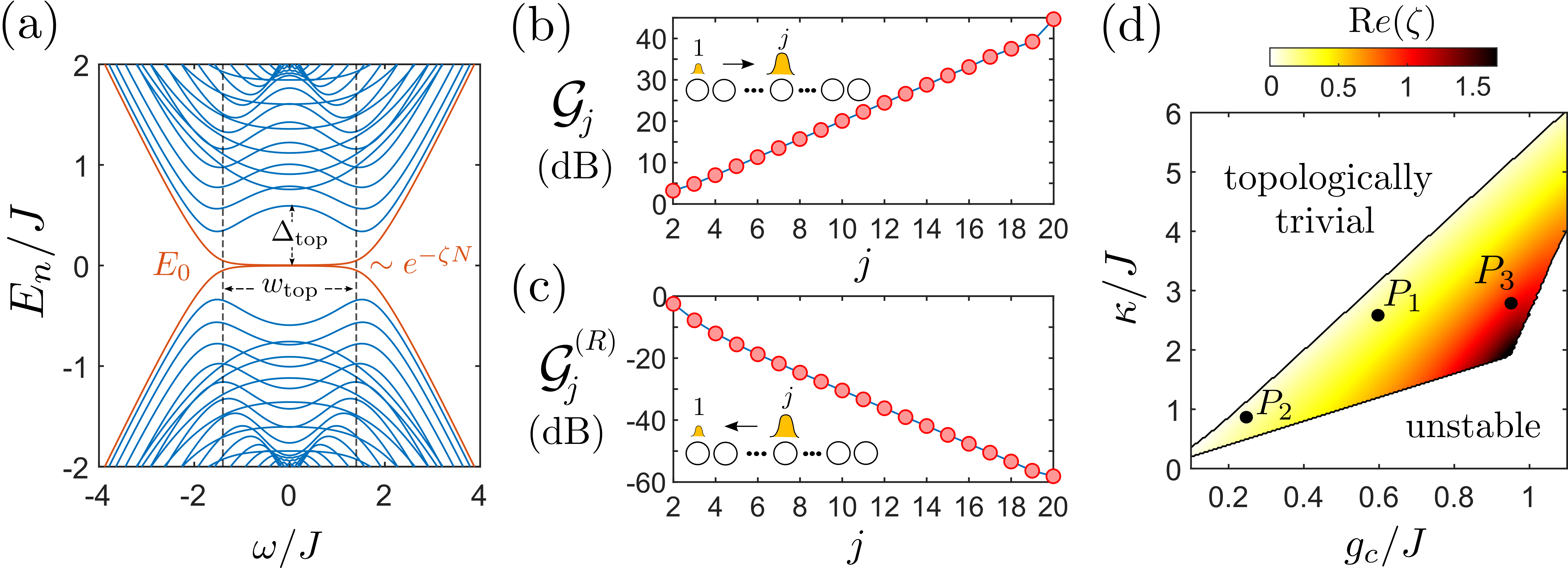
Figure 2: Directional amplification in a topological JTWPA. (a) Eigen-spectrum $E_{n}$ of the extended Hamiltonian ${\cal H}(\omega)$ in Eq. (7) as function of frequency $\omega$. In a topologically non-trivial steady state, $E_{n}(\omega)$ manifests pairs of zero-energy modes $E_{0}(\omega)\sim\pm e^{-N\zeta(\omega)}$ (in red) within a topological band-gap of size $\Delta_{\rm top}$ and a topological bandwidth $w_{\rm top}$. (b) Exponential growth of the gain ${\cal G}_{j}$ (in dB) for a signal of frequency $\omega_{s}=-0.5J$ entering at site $1$ and leaving at site $j$. (c) Exponential suppression of the reverse gain ${\cal G}_{j}^{(R)}$ (in dB) for the same signal propagating backwards from site $j$ to the first site $1$. (d) Phase diagram as function of $\kappa/J$ and $g_{c}/J$ indicating the region for stable topological steady-state phases. The color bar shows the inverse localization length ${\rm Re}[\zeta]>0$, which determines the strength of the topological amplification (see text). The black dots indicate the three operation points we consider in this work. $P_{1}$ corresponds to $g_{c}/J=0.6$ and $\kappa/J=2.6$ , $P_{2}$ to $g_{c}/J=0.25$ and $\kappa/J=0.9$, and $P_{3}$ to $g_{c}/J=0.95$ and $\kappa/J=2.8$. Other parameters are $g_{s}/g_{c}=1$, $\Delta=0$, $\phi=\pi/2$, $\omega=-0.5J$, and $N=20$. Parameters $P_{1}$ are used in panels (a)-(c).

III Directional amplification via topology

To identify the conditions under which the steady state of the system stabilizes a topological amplifying phase, we need to consider the complete driven-dissipative dynamics of the quantum fluctuations $\delta a_{j}(t)$. In the Heisenberg picture, this can be conveniently written in linear matrix form as,

$$\delta\dot{\vec{a}}(t)=-iH_{\rm nh}\delta\vec{a}(t)-\sqrt{\kappa}\vec{a}_{\rm in}(t),$$ (5)

where $\delta\vec{a}(t)=[\delta a_{j}(t),\delta a_{j}^{\dagger}(t)]^{T}$ is the vector of quantum fluctuations, and $\vec{a}_{\rm in}(t)=[a_{j}^{\rm in}(t),a_{j}^{\rm in}{}^{\dagger}(t)]^{T}$ the vector of input operators describing the signal and/or noise fields entering the amplifier at any of its sites $j$ [cf. Fig. 1(d)]. Importantly, the $2N\times 2N$ non-Hermitian matrix $H_{\rm nh}$ describes interactions, pumping, and dissipative processes in a unified way,

$$H_{\rm nh}=\begin{pmatrix}{\cal M}_{jl}-i\frac{\kappa}{2}\delta_{jl}&-{\cal K}_{jl}\\ {\cal K}_{jl}&-{\cal M}^{\ast}_{jl}-i\frac{\kappa}{2}\delta_{jl}\end{pmatrix},$$ (6)

and it contains all information about the dynamical and spectral properties of the amplifier (see Appendix C), as well as the stability and topology of the steady-state (see Appendix D). For instance, in terms of the Green’s function matrix $G(\omega)=(\omega-H_{\rm nh})^{-1}$, we can determine the amplifier’s gain ${\cal G}_{j}=\kappa^{2}|G_{j1}(\omega_{s})|^{2}$ for a signal of frequency $\omega_{s}$ entering at site $1$ and leaving at any site $j>1$. Similarly, the reverse gain from site $j>1$ to $1$ is given by ${\cal G}_{j}^{(R)}=\kappa^{2}|G_{1j}(\omega_{s})|^{2}$. Note that we are operating the device as a phase-preserving amplifier and that all frequencies $\omega$ and $\omega_{s}$ are taken with respect to the pump $\omega_{b}$.

In a topologically non-trivial steady-state phase, the Green’s function components become asymmetric, $G_{jl}\neq G_{lj}$, and therefore the amplification is non-reciprocal. To see for which parameters this indeed occurs, we rely on a connection between open quantum systems and topological band theory that we developed in Refs. [25, 27, 37]. This consists in constructing an artificial hermitian Hamiltonian ${\cal H}(\omega)$ from the non-hermitian $H_{\rm nh}$ matrix as,

$${\cal H}(\omega)=\begin{pmatrix}0&\omega-H_{\rm nh}\\ \omega-H_{\rm nh}^{\dagger}&0\end{pmatrix},$$ (7)

and relating the eigenvalue problem of ${\cal H}(\omega)$ to the true steady-state properties and Green’s functions of the amplifier array. In particular, if the system parameters are such that ${\cal H}(\omega)$ is in a topologically non-trivial phase (according to the ten-fold way [38]), its eigen-spectrum $E_{n}(\omega)$ manifests pairs of zero-energy modes whose energy is exponentially suppressed, $E_{0}(\omega)\sim\pm e^{-N\zeta(\omega)}$, with $\zeta$ the inverse localization length. As shown in Fig. 2(a), these zero-energy modes appear within a topological band-gap $\Delta_{\rm top}$ and also within a topological bandwidth $w_{\rm top}$, since the topological region is frequency dependent. Inside this region, defined as $E_{0}(\omega)\leq 1/N$ for a finite system, the associated zero-energy eigenstates of ${\cal H}(\omega)$ are exponentially localized edge states, which induce an exponential spatial dependence on the physical Green’s functions $G_{jl}(\omega)$ of the system as (see Appendix D and Ref. [39]),

$$G_{jl}(\omega)\approx e^{(j-l)\zeta(\omega)}G_{11}(\omega),\qquad j>l.$$ (8)

Directional amplification follows directly from this fact since the gain of the topological amplifier grows exponentially from left to right ${\cal G}_{j}\approx e^{2(j-2){\rm Re}(\zeta)}{\cal G}_{2}$, while back-wards propagating signals are exponentially suppressed with distance . Figs. 2(b)-(c) demonstrate numerically this behaviour for a signal of frequency $\omega_{s}=-0.5J$ and the same parameters as in Fig. 2(a). Due to the exponential scaling of the gain, a topological JTWPA of just $N=20$ sites reaches more than $40$ dB of amplification and $-60$ dB of reverse attenuation. Note that small deviations from the exponential dependence near the boundaries are due to finite size effects.

Looking for edge states in ${\cal H}(\omega)$ allows for a systematic study of the steady-state phases supporting directional amplification. Fig. 2(d) displays a phase diagram of the system as a function of $g_{c}/J$ and $\kappa/J$, for given parameters $g_{s}/g_{c}=1$, $\omega/J=-0.5$, $\Delta=0$, $\phi=\pi/2$, and $N=20$. The colored region indicates the topological amplifying phase, which requires a balance between parametric drive $g_{c}$ and decay $\kappa$: For too large decay, the system becomes topologically trivial and for too large drive it becomes unstable. Stability of the steady-state is an essential requisite for the experimental realization of the topological JTWPA, which is guaranteed when all eigenvalues of $H_{\rm nh}$ have negative imaginary parts [25, 27]. In addition, the color bar in Fig. 2(d) displays the inverse localization length ${\rm Re}[\zeta]$ which determines the exponent of the gain in the topological phase. Note that larger ${\rm Re}[\zeta]$ is not always better as this depends on the application of the amplifier. In this work, we consider three working points as indicated in Fig. 2(d). Parameters $P_{1}$ are used in panels (a)-(c) of Figs. 2, whereas $P_{2}$ and $P_{3}$ are used below when discussing the performance of the amplifier.

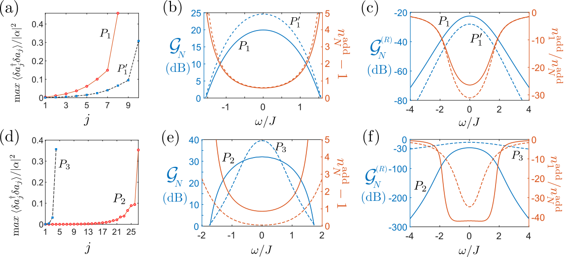
Figure 3: Broadband performance of the topological JTWPA. (a) Normalized maximum occupation $\braket{\delta a_{j}^{\dagger}(t)\delta a_{j}(t)}/|\alpha|^{2}$ as function of array site $j$ when amplifying a signal of flux $|\alpha_{s}|^{2}=0.03J$ and frequency $\omega_{s}=-0.5J$. (b) Frequency dependence of gain ${\cal G}_{N}$ (blue) and added noise above the quantum limit $n^{\rm add}_{N}-1$ (red) at the last array site $j=N$, represented on the left and right vertical axes, respectively. (c) Frequency dependence of reverse gain ${\cal G}_{N}^{(R)}$ at last site (blue) and noise asymmetry $n^{\rm add}_{1}/n^{\rm add}_{N}$ (red), represented on the left and right vertical axes, respectively. In panels (a)-(c), solid lines correspond to parameters $P_{1}$ with $N=8$ and dashed line to $P_{1}^{\prime}$ with $N=10$. (d)-(f) Same quantities as in (a)-(c) but for $|\alpha_{s}|^{2}=0.05J$, and parameters $P_{2}$ (solid) and $P_{3}$ (dashed).

IV Performance of the directional amplifier

Similarly to JPAs [41, 13], the gain of the topological JTWPA cannot grow indefinitely because quantum fluctuations become highly populated $\braket{\delta a_{j}^{\dagger}(t)\delta a_{j}(t)}\gtrsim|\alpha|^{2}$, and saturate the linear response of the system. Indeed, when amplifying a coherent signal of frequency $\omega_{s}$ entering at site $1$, the occupation at site $j>1$ oscillates in time reaching a maximum (see Appendix C):

$${\rm max}\braket{\delta a_{j}^{\dagger}\delta a_{j}}={} \kappa|\alpha_{s}|^{2}(|G_{j1}(\omega_{s})|+|G_{j,N+1}(-\omega_{s})|)^{2}$$

$$+\frac{1}{2\pi\kappa}\int d\omega n_{j}(\omega).$$ (9)

The first term is proportional to the input flux $|\alpha_{s}|^{2}$ and originates from coherent photons in signal and idler fields. In contrast, the second term describes incoherent photons generated by the amplifier with a density $n_{j}(\omega)=\kappa^{2}\sum_{l}|G_{j,N+l}(\omega)|^{2}$ per unit frequency. This noise is fundamentally bounded by $n_{j}^{\rm add}(\omega)=n_{j}(\omega)/{\cal G}_{j}(\omega)\geq 1$, with $n_{j}^{\rm add}(\omega)$ the added noise , and thus it is always present in a quantum amplifier. In the topological phase, the Green’s function anomalous components $G_{j,N+l}$ behave exponentially as $G_{jl}$ in Eq. (8) and, therefore, ${\rm max}\braket{\delta a_{j}^{\dagger}\delta a_{j}}$ also grows exponentially from left to right [cf. Fig. 3(a)]. On the one hand, this directional growth is a steady-state signature of topological amplification as it indicates the accumulation of photons at one boundary of the system [cf. Fig. 1(d)]. On the other hand, this fast growth also limits the size $N$ in which the amplifier avoids saturation, $\braket{\delta a_{N}^{\dagger}\delta a_{N}}/|\alpha|^{2}\ll 1$. Nevertheless, a compact topological JTWPA can still show an outstanding performance in all figures of merit as shown below.

Let us first consider the working point $P_{1}$ used in Fig. 2, which can be realized with circuit parameters similar to the ones in Ref. [34] (see details in Table 1 of Appendix E). For this parameter set, the device can avoid saturation up to a size of $N=8$ when amplifying a signal of $|\alpha_{s}|^{2}/2\pi\sim 5$ MHz [cf. solid line in Fig. 3(a)]. To characterize the broadband performance of the directional amplification, we display in Figs. 3(b)-(c) the frequency dependence of the gain ${\cal G}_{N}$ and reverse gain ${\cal G}^{(R)}_{N}$ (left axes in blue), as well as the added noise $n^{\rm add}_{N}$ and noise asymmetry $n^{\rm add}_{1}/n^{\rm add}_{N}$ (right axes in red). For parameters $P_{1}$ (solid lines), we find that the gain ${\cal G}_{N}$ can reach 20 dB at the center with just 0.6 added photons above the quantum limit. Within the topological bandwidth of $w_{\rm top}\sim 2J=2\pi\cdot 310$ MHz, the gain is above 13 dB, reverse gain below -23 dB, and noise asymmetry below -22 dB, providing a strong protection to the quantum source that generates the signal. For a directional amplifier, this bandwidth is already one order of magnitude larger than what has been achieved so far [16, 17, 18, 19, 20, 21], but for practical application it is desirable to provide at least 20 dB of gain over a bandwidth of GHz [15]. We show below that this is possible for a topological JTWPA provided one uses a technique already developed for JPAs.

Increasing the gain, bandwidth, and dynamic range boils down to increasing the maximum $|\alpha|^{2}$ that the system can sustain, but this is fundamentally restricted in JJ arrays by the low flux condition $|\phi_{j}^{a}|\ll\Phi_{0}$, which implies $|\alpha|^{2}\ll(\Phi_{0}/2\phi_{zpf})^{2}$ [13, 33], with $\Phi_{0}$ the flux quantum and $\phi_{zpf}$ the zero point fluctuation (see Appendix A). Since $\phi_{zpf}=\sqrt{\hbar/(2\omega_{a}C_{a}^{\rm eq})}$, the naive solution is to increase the capacitance $C_{a}^{\rm eq}$ further, but in practice this is problematic as it generates parasitic geometrical inductances larger than the Josephson inductances themselves. Nevertheless, as proposed and experimentally demonstrated in Refs. [13, 33, 41], we can replace each JJ in the setup [cf. Fig. 1(a)] by a sub-array of $M$ JJs in series (with a Josephson energy $M$ times larger), and thereby reduce the flux drop across each JJ as $\phi_{j}^{a}\rightarrow\phi_{j}^{a}/M$ (see Fig. 5(b) of Appendix A). Remarkably, this allows the topological JTWPA to sustain a mean displacement $M^{2}$ times larger, $|\alpha|^{2}\ll M^{2}(\Phi_{0}/2\phi_{zpf})^{2}$, while keeping the same effective quantities in Eq. (4).

Implementing these sub-arrays of JJs has a dramatic improvement in the performance of the topological JTWPA. To show this, we consider circuit parameters similar to the ones reported in Ref. [33] that realize the same effective parameters $P_{1}$ used in Fig. 2. We call these parameters $P_{1}^{\prime}$ as detailed in Table 1 of Appendix E. If we consider $M=7$, the topological JTWPA can sustain $|\alpha|^{2}=175$ photons and avoids the saturation regime up to $N=10$ sites [cf. dashed line in Fig. 3(a)]. As shown in Fig. 3(b)-(c) (dashed lines), having just two more sites compared to $P_{1}$ boosts the gain to ${\cal G}_{N}\sim 25$ dB at the center frequency, the reverse gain to $-28$ dB, and the noise asymmetry to $-30$ dB, while keeping the same near-quantum limited added noise. Importantly, this also improves the bandwidth since the directional amplifier now provides more than $20$ dB of gain over $\Delta\omega_{20}\sim 1.7J\sim 2\pi\cdot 265$ MHz.

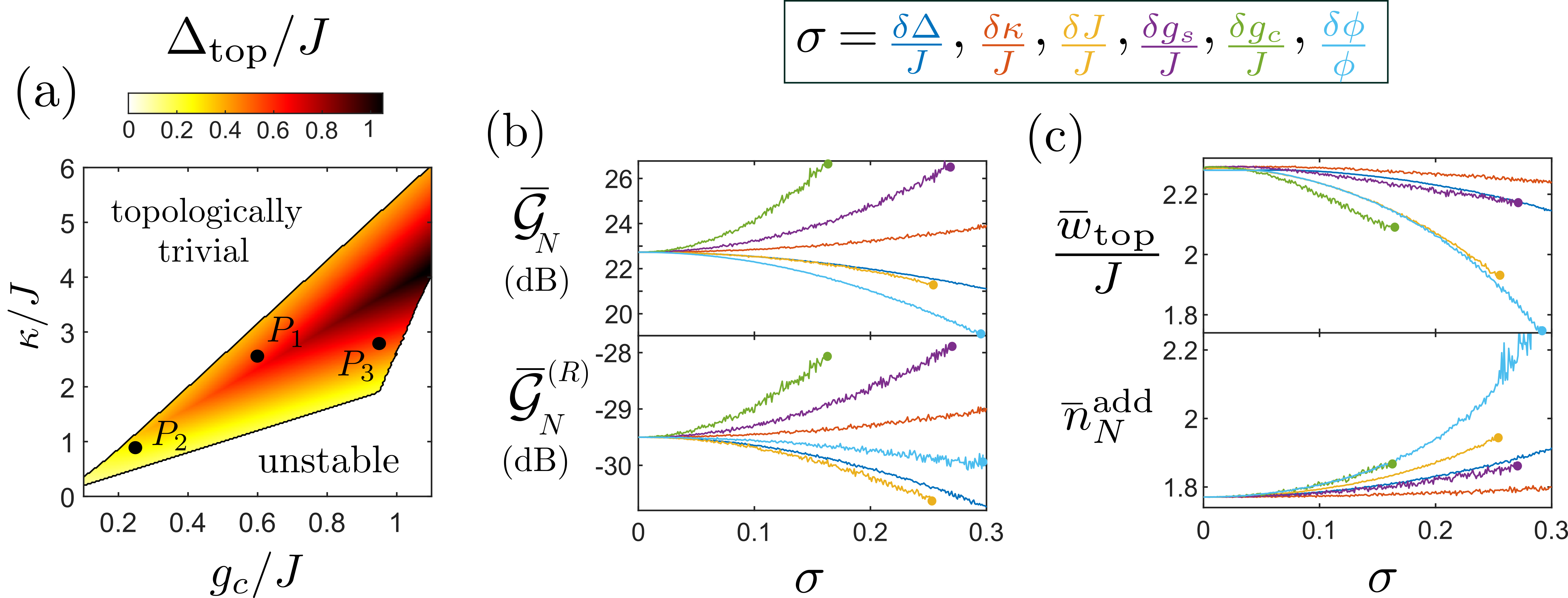
Figure 4: Robustness against disorder in all system parameters. (a) Topological gap $\Delta_{\rm top}/J$ as function of $\kappa/J$ and $g_{c}/J$ for the same parameters and same stable topological region as in Fig. 2(d). The black dots indicate the position of the three operation points discussed in this work. (b)-(c) Average gain $\bar{{\cal G}}_{N}$, reverse gain $\bar{{\cal G}}_{N}^{(R)}$, topological bandwidth $\bar{w}_{\rm top}/J$, and added noise $\bar{n}_{\rm add}^{N}$ as function of the dimensionless disorder strength $\sigma$, defined for each system parameter as $\sigma=\delta\Delta/J$ (blue), $\sigma=\delta\kappa/J$ (red), $\sigma=\delta J/J$ (yellow), $\sigma=\delta g_{s}/J$ (purple), $\sigma=\delta g_{c}/J$ (green), and $\sigma=\delta\phi/\phi$ (cyan). All quantities are averaged over 3000 realizations for each type of disorder around the mean values defined by parameters $P_{1}^{\prime}$ (corresponding to $P_{1}$ with $N=10$, see Table 1). The signal frequency is set to $\omega_{s}=-0.5J$. Colored dots at the end of curves indicate the disorder $\sigma$ from which the steady-state becomes unstable.

Reaching a bandwidth on the order of GHz, requires increasing the effective hopping $J=J_{a}+2g_{c}$ of the device. Unfortunately $g_{c}=K_{c}|\alpha|^{2}$ is limited by the low flux condition and cannot be increased with $M$ , but we can increase $J$ via $J_{a}$ at the expense of reducing the ratio $g_{c}/J$. In particular, we consider parameters $P_{2}$ with $g_{c}/J=0.25$ and $\kappa/J=0.9$, which lies within the stable topological region as shown in Fig. 2(d). At this working point, the inverse localization length reads ${\rm Re}[\zeta]\sim 0.1$, which is around half that for $P_{1}$. This slows down the exponential growth of the gain, but an excellent performance can still be obtained with a slightly larger $N$ since ${\cal G}_{N}\propto e^{2N{\rm Re}[\zeta]}$. Using realistic circuit parameters similar to Ref. [33] (see Table 1 of Appendix E), we show in Fig. 3(d) (dashed line) that the device at $P_{2}$ can safely avoid saturation up to $N=27$ sites, with $M=32$ and an input flux of $|\alpha_{s}|^{2}/2\pi\sim 19$ MHz. Since $J/2\pi=375$ MHz the topological amplifier now provides more than 20 dB of gain over a bandwidth of $\Delta\omega_{20}\approx 2.7J\approx 2\pi\cdot 1.01$ GHz, reaching a maximum of ${\cal G}_{N}=32$ dB at the center [cf. Fig. 3(e), blue solid line]. Due to the smaller ${\rm Re}[\zeta]$, the added noise has slightly increased compared to $P_{1}$, but over the whole bandwidth $\Delta\omega_{20}$ it is still below 2.7 photons above the quantum limit (and 0.9 at the center) [cf. Fig. 3(e), red solid line]. Regarding directionality, the reverse gain is below -29 dB, and noise asymmetry stays nearly flat at -40 dB [cf. Fig. 3(f), solid lines].

We see that for parameters of type $P_{2}$, the topological JTWPA becomes a truly broadband and directional amplifier for microwave signals. Achieving these outstanding numbers requires building a superconducting chip with a total of $N_{JJ}=(2N+1)M=1760$ JJs, which is less than what has been utilized in non-directional JTWPAs [9, 12]. Also, note that the case $N=2$ and $M=30$ was experimentally implemented in Ref. [33], but without cross-Kerr coupling and therefore the device was operated as a JPA.

The topological JTWPA is very versatile and it can also be used as an ultra-low noise directional amplifier at the expense of losing bandwidth. This requires ${\rm Re}[\zeta]\gg 1$, since then the added noise becomes exponentially close to the quantum limit: $n^{\rm add}_{N}(\omega)\approx 1+e^{-2{\rm Re}[\zeta(\omega)]}$. For this, we consider the last operation point $P_{3}$, for which ${\rm Re}[\zeta]\sim 1$ as indicated in Fig. 2(d). The dashed lines of Figs. 3(d)-(f) display all the corresponding figures of merit. Due to extreme localization of the edge states, we see that a device with only $N=4$ and $M=22$ already reaches the same degree of saturation as $P_{2}$ with $N=27$. Remarkably, near the pump frequency $\omega\sim 0$, the gain can reach 40 dB with only 0.06 photons above the quantum limit. This great performance can be maintained over a bandwidth of $\Delta\omega_{20}\sim 2J\sim 2\pi\cdot 200$ MHz with gains above 20 dB and added noise below 1.4. Reducing the noise further requires to be closer to the instability region, but operating the device gets increasingly difficult. Reverse gain is maximum -10 dB which is worse than the other cases due to the smallness of the device with $N=4$. Increasing $N$ is possible but requires a large $M$ to reduce saturation.

Throughout the performance analysis, we have considered input signals with moderate intensity $|\alpha_{s}|^{2}/2\pi<20$ MHz in order to safely neglect saturation effects, but it is possible to increase the input power much further. We estimate that reaching $|\alpha_{s}|^{2}/2\pi\sim 320$ MHz or 2000 photons per $\mu s$ (as reported for a JPA [33]) requires a topological amplifier with $M\sim 45$ when operating at the optimal point before saturation $\braket{\delta a_{N}^{\dagger}(t)\delta a_{N}(t)}\lesssim|\alpha|^{2}$. These are still less JJs per site than the JPA with $M=80$ that was recently realized [41]. However, making a precise estimation of the dynamic range requires modeling the non-linear processes present in the device [41, 13], and this is left for future work. In addition, we note that the pump frequency $\omega_{b}$ sets the central frequency of the amplifier’s response in Figs. 3 and this has been assumed fixed. By replacing all JJs in the setup by SQUIDS [41, 13], the topological JTWPA becomes flux-tunable and it can amplify signals in the whole GHZ range.

V Topological protection against disorder

The last remarkable property of the topological JTWPA is the robustness to disorder, which can highly facilitate its experimental realization with current superconducting circuit technology. The origin of the topological protection lies in the presence of an intrinsic chiral symmetry of the extended Hamiltonian ${\cal H}(\omega)$ in Eq. (7), and in the robustness of the breaking of TRS via $\phi=\pi/2\neq 0$. Smooth changes due to disorder cannot modify the symmetry class of the edge states of ${\cal H}(\omega)$, and the topological steady-state phase persists as long as the disorder strength is smaller than the gap, $\delta x\ll\Delta_{\rm top}$ [25, 27, 44]. Here, $\delta x$ denotes the standard deviation of any system quantity $x$, assumed to be normally distributed around the mean values discussed in previous sections. Note that for robust breaking of TRS we also require that the disorder in the phase fulfills $\delta\phi\ll\phi$.

Fig. 4(a) displays the topological gap $\Delta_{\rm top}/J$ for the same topological phase shown in Fig. 2(d). We see that the gap grows with $g_{c}/J$ and decreases towards the border of the phase . Therefore, topological protection is optimal at the middle of the topological phase, where the gap is large $\Delta_{\rm top}/J>0.3J$ and the steady-state is far from the instability region. Here is where we have placed the three operation points $P_{1}$-$P_{3}$ [cf. 4(a)]. In the following we demonstrate the robustness of the topological JTWPA at $P_{1}^{\prime}$. The behavior for $P_{2}$ is similar and for $P_{3}$ is slightly less robust due to the larger ${\rm Re}[\zeta]$ (see Appendix F).

In Figs. 4(b)-(c) we show the average gain $\bar{{\cal G}}_{N}$, reverse gain $\bar{{\cal G}}^{(R)}_{N}$, topological bandwidth $\bar{w}_{\rm top}$, and added noise $\bar{n}_{N}^{\rm add}$ as function of the dimensionless disorder strength $\sigma=\delta x/J$ for all effective system parameters $x=\Delta$ (blue), $x=\kappa$ (red), $x=J$ (yellow), $x=g_{s}$ (purple), and $x=g_{c}$ (green), as well as for the phase $\sigma=\delta\phi/\phi$ (cyan). The frequency of the input signal is set to $\omega_{s}=-0.5J$. We see that for $\sigma\lesssim 5\%$, none of the figures of merit are appreciably affected. For a larger disorder between $\sim 5\%$ and $\sim 30\%$ the topological amplification is preserved but its performance is modified. The amplifier’s noise $\bar{n}^{\rm add}_{N}$ slightly increases and the topological bandwidth $\bar{w}_{\rm top}$ shrinks. However, some types of disorder such as $\delta g_{c,s}$ and $\delta\kappa$ can enhance the gain $\bar{{\cal G}}_{N}$ at the expense of reducing directionality in $\bar{{\cal G}}^{(R)}_{N}$. This noise-induced effect is reminiscent to topological Anderson insulators observed in photonic systems [46], where noise re-normalizes the system parameters and can even trigger topological phase transitions. For even larger disorder $\sigma\simeq 1$, the gain always reduces and directional topological amplification is lost (see Appendix F).

In addition, disorder can destabilize the amplifying steady-state depending on the operation point and/or disorder type. For $P_{1}^{\prime}$, the early termination of certain curves in Figs. 4(b)-(c) indicates the specific disorder strength at which the system becomes unstable. Including this stability analysis, we predict an overall tolerance to disorder of at least $\sigma\lesssim 10\%$ in all system parameters, while retaining the excellent performance of the directional amplification. A practical implementation of the topological JTWPA will be mainly affected by disorder and inhomogeneties inherent to the fabrication of JJs [32] and this constitutes a natural protection against it.

VI Conclusions and outlook

We have presented a radically new design of a JTWPA that exploits non-Hermitian topological effects to work in a regime of high directional gain, near quantum-limited noise, and broad bandwidth. This topological amplifier can be immediately implemented with state-of-art superconducting technology as it only requires a JJ array with few sites, 50$\Omega$ input/output ports, and an auxiliary resonator array to distribute a collective four-wave mixing pump with spatially varying phase. This quantum device can be directly integrated on-chip and used as a directional broadband pre-amplifier, alleviating the need for bulky isolators to protect the quantum source, and facilitating the control of large-scale quantum processors [15].

Our work opens several routes for exploring further technological applications, as well as the fundamental physics of topologically driven-dissipative systems. The topological JTWPA can be applied, for instance, for efficient multiplexed readout of multiple superconducting qubits [8, 22] or broadband detection of itinerant single-photons [47]. Saturation effects appearing in the device [13, 41, 48] can lead to novel regimes of operation, which can be systematically addressed by approximations like mean-field or Matrix Product State techniques.

From a more fundamental perspective, our proposal is also a versatile platform for the quantum simulation of open quantum systems [35, 49], non-Hermitian physics [50, 51], and novel topological driven-dissipative phases of matter [52, 53], including those with disorder [54] and strong photon-photon interactions [55, 56]. For quantum simulation, a particularly convenient aspect of our design is that the strength of the synthetic gauge field [28] and the nonlinear interactions can be conveniently controlled via the external pump, without requiring Floquet engineering [29] or external magnetic fields.

Appendix A Superconducting circuit model

A.1 Josephson junction array coupled to auxiliary array

We provide the detailed superconducting circuit design to implement the topological JTWPA, as well as the connection between the effective model of the main text and the microscopic circuit quantities. As shown in Fig. 5(a), at each node $j$ of the circuit we define a flux variable $\phi_{j}^{\mu}(t)$, with index $\mu=a$ corresponding to the JJ array and $\mu=b$ to the auxiliary linear array. These fluxes couple via Josephson junctions and capacitances and their dynamics is governed by the Langrangian $L=L_{\rm JJA}+L_{\rm aux}$, where

$$L_{\rm JJA}={} \sum_{j}\frac{C_{a}}{2}(\dot{\phi}_{j}^{a})^{2}+\frac{C_{a}^{\prime}}{2}\sum_{j}(\dot{\phi}^{a}_{j+1}-\dot{\phi}^{a}_{j})^{2}$$ (10)

$$+{} E_{J}\sum_{j}\cos\left(\frac{\phi_{j}^{a}}{\Phi_{0}}\right)+E_{J}^{\prime}\sum_{j}\cos\left(\frac{\phi^{a}_{j+1}-\phi^{a}_{j}}{\Phi_{0}}\right),$$

$$L_{\rm aux}={} \sum_{j}\frac{C_{b}}{2}(\dot{\phi}^{b}_{j})^{2}-\sum_{j}\frac{(\phi^{b}_{j})^{2}}{2L_{b}}+\frac{C_{b}^{\prime}}{2}\sum_{j}(\dot{\phi}^{b}_{j+1}-\dot{\phi}^{b}_{j})^{2},$$

$$+{} \sum_{j}\frac{C_{ab}}{2}(\dot{\phi}^{b}_{j}-\dot{\phi}^{a}_{j})^{2}.$$ (11)

Regarding the JJ array, we consider on-site and inter-site capacitances denoted by $C_{a}$ and $C_{a}^{\prime}$, respectively, as well as on-site and inter-site Josephson junctions, which induce nonlinear potentials with Josephson energies $E_{J}$ and $E_{J}^{\prime}$, respectively. In addition, $\Phi_{0}=\hbar/(2e)$ denotes the reduced flux quantum. In the auxiliary chain, superconducting linear resonators are realized at each node $j$ by LC circuits with capacitance $C_{b}$ and inductance $L_{b}$. These resonators are coupled via inter-site capacitances $C_{b}^{\prime}$ and also couple to the JJ array via an inter-array capacitance $C_{ab}$. The left- and right-most sites of the array are coupled to ground which provides the boundary conditions, $\phi_{0}^{\mu}=\phi_{N+1}^{\mu}=0$.

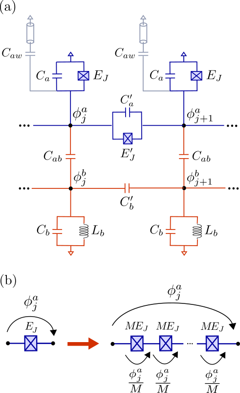
Figure 5: Detailed circuit diagram for two adjacent sites of the topological JTWPA. (a) Flux variables $\phi_{j}^{\mu}$ are defined at each node of the circuit given by the chain index $\mu=a,b$ and the position $j$. The JJ array (blue) is composed of on-site and inter-site JJs with Josephson energies $E_{J}$ and $E_{J}^{\prime}$, as well as capacitances $C_{a}$ and $C_{a}^{\prime}$. Each site of the JJ array is additionally coupled to a $50\Omega$ transmission line with capacitance $C_{aw}$ (grey). Finally, the JJ array also couples via a capacitance $C_{ab}$ to a linear array of superconducting resonators (red), given by LC circuits with on-site capacitance $C_{b}$ and inductance $L_{b}$. These resonators are also coupled by inter-site capacitances $C_{b}^{\prime}$. (b) Optional upgrade for the topological JTWPA to increase its dynamic range. It consists in replacing all intra- and inter-site JJs in the array (a) by a sub-array of $M$ JJs in series. Increasing $E_{J},E_{J}^{\prime}\rightarrow ME_{J},ME_{J}^{\prime}$ reduces the flux drop along each JJ by a factor $M$, and thereby increases by a factor $M^{2}$ the photons that the system can sustain before saturation [13, 33].

We consider the low flux regime, $|\phi_{j}^{a}|\ll\Phi_{0}$, so that the nonlinear JJ potentials can be expanded as $\cos(x)=1-x^{2}/2+x^{4}/24+{\cal O}(x^{6})$, and the JJ array behaves as a weakly anharmonic resonator array with self- and cross-Kerr couplings coming from the fourth order terms $\sim(\phi_{j}^{a})^{4}$ and $\sim(\phi_{j+1}^{a}-\phi_{j}^{a})^{4}$. Following the canonical quantization procedure [4, 56], we can express the flux $\phi_{j}^{\mu}$ and charge $q_{j}^{\mu}=\partial L/\partial\dot{\phi}_{j}^{\mu}$ variables in terms localized bosonic modes $a_{j}$ and $b_{j}$, for the JJ and auxiliary arrays, respectively. The coherent dynamics of these modes is described by the total Hamiltonian, $H=H_{\rm JJA}+H_{\rm JJA}^{\prime}+H_{\rm aux}$, with $H_{\rm JJA}$ and $H_{\rm aux}$ given in Eqs. (1)-(2), and $H_{\rm JJA}^{\prime}=\frac{K_{c}}{4}\sum_{j}[2(a_{j}^{\dagger})^{2}a_{j}a_{j+1}+2a_{j}^{\dagger}a_{j+1}^{\dagger}(a_{j+1})^{2}-(a_{j}^{\dagger})^{2}(a_{j+1})^{2}+{\rm h.c.}]$. This extra Hamiltonian term $H_{\rm JJA}^{\prime}$ does not qualitatively change the dynamics of the JJ array, but it must be included to obtain the proper parametric amplifier Hamiltonian in Eq. (4).

Regarding the effective parameters of the model, the on-site frequency of the JJ array modes reads $\omega_{a}=(L_{a}^{\rm eq}C_{a}^{\rm eq})^{-1/2}$, with $C_{a}^{\rm eq}=C_{a}+2C_{a}^{\prime}+C_{ab}$ the equivalent capacitance and $L_{a}^{\rm eq}=(L_{J}^{\prime}L_{J})/(L_{J}^{\prime}+2L_{J})$ the equivalent inductance. Here, $L_{J}=\Phi_{0}^{2}/E_{J}$ and $L_{J}^{\prime}=\Phi_{0}^{2}/E_{J}^{\prime}$ are the on-site and inter-site Josephson inductances, respectively. In addition, the linear hopping in the JJ array contains capacitive and inductive contributions $J_{a}=\frac{\omega_{a}}{2}(C_{a}^{\prime}/C_{a}^{\rm eq}-L_{a}^{\rm eq}/L_{J}^{\prime})$, whereas the the self- and cross-Kerr coupling strengths read $K_{s}=E_{C}/\hbar$ and $K_{c}=2(E_{C}/\hbar)(L_{a}^{\rm eq}/L_{J}^{\prime})$, with $E_{C}=e^{2}/(2C_{a}^{\rm eq})$ the charging energy. Regarding the auxiliary chain, the on-site frequency reads $\omega_{b}=(L_{b}C_{b}^{\rm eq})^{-1/2}$, with $C_{b}^{\rm eq}=C_{b}+2C_{b}^{\prime}+C_{ab}$ its equivalent capacitance. The intra-array and inter-array linear hoppings are purely capacitive and take the form $J_{b}=\frac{\omega_{b}}{2}(C_{b}^{\prime}/C_{b}^{\rm eq})$ and $J_{ab}=\frac{\sqrt{\omega_{a}\omega_{b}}}{2}C_{ab}(C_{a}^{\rm eq}C_{b}^{\rm eq})^{-1/2}$, respectively. We note to derive $H$, we neglect long-range capacitive couplings provided $C_{a}^{\prime},C_{ab}\ll C_{a}^{\rm eq}$ and $C_{b}^{\prime},C_{ab}\ll C_{b}^{\rm eq}$, and we apply the rotating wave approximation, provided all couplings are much smaller than the on-site frequencies $\omega_{a}$ and $\omega_{b}$. Note that Kerr-couplings induce small shifts $\omega_{a}\rightarrow\omega_{a}-K_{c}-K_{s}$ and $J_{a}\rightarrow J_{a}+K_{c}$. Finally, the low flux approximation does not only require $E_{C}\ll E_{J},E_{J}^{\prime}$ as for transmons [4]. As shown in Ref. [13], we also require that the mean number of excitations on each site is bounded as $|\alpha_{j}|^{2}\ll(\Phi_{0}/2\phi_{\rm zpf})^{2}$, with $\phi_{\rm zpf}=\sqrt{\hbar/(2C_{a}^{\rm eq}\omega_{a})}$ the zero flux fluctuation of the JJ array. This limits the dynamic range of the device, but as demonstrated in Refs. [13, 33, 41], we can replace each JJ in the setup by a sub-array of $M$ JJs in series to increase the upper bound by a factor $M^{2}$. This requires increasing the Josephson energies as $E_{J},E_{J}^{\prime}\rightarrow ME_{J},ME_{J}^{\prime}$ such that the phase drop on each intra- and inter-site JJ reduces by a factor $M$ [cf. Fig. 5(b)]. Notice, however, that the total phase drop along each sub-array remains the same and therefore all linear circuit parameters are unchanged except for the Kerr non-linearities, which reduce as $K_{c},K_{s}\rightarrow K_{c}/M^{2},K_{s}/M^{2}$ [13].

A.2 Input/output ports, dissipation, and coherent pump

Input/output ports are realized by standard transmission lines with $Z_{0}=50\Omega$ impedance. As shown in Figs. 1(a) and 5(a), we couple one of these lines to each site of the JJ array with capacitance $C_{aw}$, as well as to the boundaries of the auxiliary array, $j=1$ and $j=N$, with a different capacitance $C_{bw}$. Assuming a Markovian coupling, the local decay rate induced on each site of the JJ array is given by $\kappa=(C_{wa}/C_{a}^{\rm eq})^{2}(Z_{0}/Z_{a})(\omega_{a}/2)$ [4, 49], with $Z_{a}=\sqrt{L_{a}^{\rm eq}/C_{a}^{\rm eq}}$ the impedance of the JJ array. Similarly, the decay rate induced on the boundaries of the auxiliary chain reads $\Gamma=(C_{wb}/C_{b}^{\rm eq})^{2}(Z_{0}/Z_{b})(\omega_{b}/2)$, with $Z_{b}=\sqrt{L_{b}^{\rm eq}/C_{b}^{\rm eq}}$. Notice that the coupling to the transmission lines renormalizes the equivalent capacitances of the JJ array as $C_{a}^{\rm eq}\rightarrow C_{a}^{\rm eq}+C_{aw}$. For the auxiliary chain, this change is compensated by choosing a slightly lower capacitance $C_{b}\rightarrow C_{b}+C_{b}^{\prime}-C_{bw}$ only at the boundaries, $j=1$ and $j=N$.

In addition, we use the input port on the first auxiliary site $j=1$ to perform a strong and resonant coherent drive only on mode $b_{1}$. This is described by Hamiltonian $H_{b}^{(p)}=2i\Omega_{b}\cos(\omega_{b}t)(b_{1}+b_{1}^{\dagger})$, with $\Omega_{b}=(C_{wb}/2C_{b}^{\rm eq})\sqrt{Z_{0}/Z_{b}}\sqrt{P_{b}/\hbar}$ the driving strength and $P_{b}$ the pump power [4].

Appendix B Four-wave mixing via auxiliary array

B.1 Displacement on quantum Langevin equations and perfect phase matching via phase of non-local pump

The complete driven-dissipative dynamics of the two coupled arrays is given by the quantum Langevin equations,

$$\dot{a}_{j}={} i[H^{\prime},a_{j}]-\frac{\kappa}{2}a_{j}-\sqrt{\kappa}a^{\rm in}_{j}(t),$$ (12)

$$\dot{b}_{j}={} i[H^{\prime},b_{j}]-\left(\frac{\Gamma}{2}b_{j}+\sqrt{\Gamma}b^{\rm in}_{j}(t)\right)(\delta_{j1}+\delta_{jN}),$$ (13)

where $H^{\prime}=H+H_{b}^{(p)}$ contains all coherent couplings and the driving on the first site of the auxiliary array. In addition, $a_{j}^{\rm in}(t)$ and $b^{\rm in}_{j}(t)$ describe the vacuum input fields at site $j$ of the JJ and auxiliary arrays, respectively. For a strong pump, we can do four-wave-mixing and displace all coupled modes as $a_{j}(t)=(\alpha+\delta a_{j}(t))e^{-i(\phi j+\omega_{b}t)}$ and $b_{j}=(\beta_{j}+\delta b_{j}(t))e^{-i\omega_{b}t}$, where $\delta a_{j}$ and $\delta b_{j}$ are quantum fluctuations around the large mean displacements $\alpha$ and $\beta_{j}$, respectively. Using the previous ansatz in Eqs. (12)-(13), we find classical coupled equations for the mean displacements,

$$\dot{\alpha}={} -\left(\frac{\kappa}{2}-i(A+B|\alpha|^{2})\right)\alpha-iJ_{ab}\beta_{j}e^{i\phi j},$$ (14)

$$\dot{\beta}_{j}={} -\sum_{l}{\cal I}_{jl}\beta_{l}+\Omega_{b}(1+e^{2i\omega_{b}t})\delta_{j1}-iJ_{ab}\alpha e^{-i\phi j},$$ (15)

where $A=\omega_{b}-\omega_{a}-2J_{a}\cos(\phi)$, $B=K_{s}+K_{c}[2+\cos(2\phi)-4\cos(\phi)]$, and ${\cal I}_{jl}$ are matrix elements given by ${\cal I}_{jl}=\frac{\Gamma}{2}\delta_{jl}(\delta_{j1}+\delta_{jN})+iJ_{b}(\delta_{l,j+1}+\delta_{l,j-1})$. Notice that we have assumed an homogeneous mean displacement $\alpha$ for the JJ array, which can only be a valid solution if $\beta_{j}\sim e^{-i\phi j}$ and thereby cancels the $j$-dependence in the last term in Eq. (14). Here, we show that this is indeed the case for the steady-state of the system if $\Gamma=2J_{b}$ because this realizes perfect impedance matching at the boundaries of the auxiliary chain. In particular, when $\Gamma=2J_{b}$, the matrix $I_{jl}$ can be inverted exactly as $[I^{-1}]_{jl}=e^{-i(\pi/2)|j-l|}/(2J_{b})$ [57], and therefore we can solve for the steady-state solution ($t\rightarrow\infty$) of Eq. (15) as,

$$\beta_{j}=\frac{i\Omega_{b}}{2J_{b}}e^{-i(\pi/2)j}-i\frac{J_{ab}}{2J_{b}}\alpha\sum_{l}e^{-i(\phi l+\pi/2|j-l|)}.$$ (16)

Note that we have neglected fast oscillations due to the non-RWA driving term $\sim e^{2i\omega_{b}t}$ in Eq. (15), provided $J_{b},J_{ab}\ll\omega_{b}\lesssim\Omega_{b}$. Replacing Eq. (16) in (14), we see that $\beta_{j}$ induces an effective driving with stregth $\Omega_{a}=(J_{ab}/2J_{b})\Omega_{b}$ on the JJ array, and its phase $\phi=\pi/2$ provides perfect phase matching. As a result, the steady state displacement $\alpha$ satisfies a nonlinear Duffing oscillator equation [13, 41],

$$(\kappa/2-i[\omega_{b}-\omega_{a}+(K_{c}+K_{s})|\alpha|^{2}])\alpha=\Omega_{a},$$ (17)

provided we neglect non-local dissipative processes originated by the second term of the auxiliary displacement in Eq. (16). This is justified when the associated decay rate $\kappa_{\rm nl}=J_{ab}^{2}/(2J_{b})$ is much smaller than all other effective quantities $\Omega_{a},\kappa,|\omega_{b}-\omega_{a}|,(K_{s}+K_{c})|\alpha|^{2}$. Notice that the presence of additional local decay on the auxiliary cavities $b_{j}$ deteriorates the perfect absorbing condition, but the topological steady state phase is robust as long as this unwanted decay is much smaller than $J_{b}$.

B.2 Effective dynamics for quantum fluctuations

Regarding the dynamics of the quantum fluctuations $\delta a_{j}$ and $\delta b_{j}$, we see that they decouple when being far detuned, $J_{ab},J_{b}\ll|\omega_{b}-\omega_{a}|$. Under these conditions and assuming a strong displacement $|\alpha|^{2}\gg\braket{\delta a_{j}^{\dagger}\delta a_{j}}$, it is possible to derive an effective linear dynamics for the fluctuations $\delta a_{j}(t)$ of the JJ array as

$$\delta\dot{a_{j}}={} i[H_{\rm pa},\delta a_{j}]-\frac{\kappa}{2}\delta a_{j}-\sqrt{\kappa}a^{\rm in}_{j}(t)+{\cal O}(|\alpha|\delta a_{j}^{3}),$$ (18)

where $H_{\rm pa}$ is the topological parametric amplifier Hamiltonian given in Eq. (4) with effective quantities $J=J_{a}+2K_{c}|\alpha|^{2}$, $g_{c}=K_{c}|\alpha|^{2}$, and $g_{s}=(K_{c}-K_{s})|\alpha|^{2}$. The nonlinear interactions of order $\sim|\alpha|\delta a_{j}^{3}$ or higher are responsible for saturation effects in the amplifier and therefore $|\alpha|^{2}$ should be as large as possible, only limited by the low flux condition.

B.3 Analytical solution for mean photon displacement

The third-order non-linear equation (17) for the mean steady-state displacement $|\alpha|^{2}$ admits analytical solutions. In particular, for $\Delta=0$ as it is of interest in this work, we have that $|\alpha|^{2}=[\kappa/(K_{s}+K_{c})]n$ and $\omega_{b}-\omega_{a}=-2\kappa n$, where $n$ is a real solution of the third order equation, $n^{3}+n/4=\xi$, which reads

$$n(\xi)=\frac{3^{1/3}(36\xi+\sqrt{3+1296\xi^{2}})^{2/3}-3^{2/3}}{6(36\xi+\sqrt{3+1296\xi^{2}})^{1/3}}.$$ (19)

Here, the dimensionless parameter $\xi=(|\Omega_{a}|/\kappa)^{2}[(K_{s}+K_{c})/\kappa]$ controls the size of $n$, specially via the pump power $P_{b}$ on the auxiliary array which determines the effective driving strength on the JJ array, $\Omega_{a}=(J_{ab}/J_{b})(C_{wb}/2C_{b}^{\rm eq})\sqrt{Z_{0}/Z_{b}}\sqrt{P_{b}/\hbar}$. In contrast to a single-site JPA [13], the topological JTWPA has no instability at $\xi>1/\sqrt{27}$ and it can go much further in $n$, as long as the combination of the effective quantities in Eqs. (5)-(6) give a stable steady-state. This is because the equation for the fluctuations of the topological JTWPA is different than for a JPA, although the nonlinear equation for the mean-field displacement $|\alpha|^{2}$ is the same.

Appendix C Spectral properties of the amplifier from Green’s functions

In this appendix, we show how to obtain all spectral properties of the amplifier such as gain, reverse gain, and noise from the information contained in the Green’s function $G(\omega)=(\omega-H_{\rm nh})^{-1}$, where $H_{\rm nh}$ is the non-Hermitian matrix defined in Eq. (6). We also show that signal ($\omega=\omega_{s}$) and idler ($\omega=-\omega_{s}$) fields have the same topological amplifying properties.

The output operator $\bar{a}^{\rm out}_{j}(t)$ characterizes the amplified field leaving the device at the output port $j$. In the rotating frame with the pump frequency $\omega_{b}$, this is related to the input field by a standard input-output relation [4],

$$\bar{a}_{j}^{\rm out}(t)=\bar{a}_{j}^{\rm in}(t)+\sqrt{\kappa}(\alpha+\delta a_{j}(t))e^{-i\phi j}.$$ (20)

Here, $\bar{a}_{j}^{\rm in}(t)=e^{-i\phi j}a_{j}^{\rm in}(t)$, with $a_{j}^{\rm in}(t)$ the input operator in Eq. (5).

Since the Langevin equations (5) are linear, we can solve them exactly in Fourier space. Defining the Fourier transform of the fluctuation and input operators as $\delta a_{j}(\omega)=(2\pi)^{-1/2}\int dte^{i\omega t}\delta a_{j}(t)$ and $a_{j}^{\rm in}(\omega)=(2\pi)^{-1/2}\int d\omega e^{i\omega t}\delta a_{j}^{\rm in}(t)$, we have

$$\delta a_{j}(\omega)={} -i\sqrt{\kappa}\sum_{l}G_{jl}(\omega)e^{i\phi l}\bar{a}_{l}^{\rm in}(\omega)$$ (21)

$$-i\sqrt{\kappa}\sum_{l}G_{j,N+l}(\omega)e^{-i\phi l}\bar{a}_{l}^{\rm in}{}^{{\dagger}}(-\omega),$$

where $G_{jl}(\omega)$ and $G_{j,N+l}(\omega)$ are the normal and anomalous components of the $2N\times 2N$ Green’s function matrix $G(\omega)=(\omega-H_{\rm nh})^{-1}$.

To characterize the amplifying properties of the device, we measure the output field $\bar{a}_{j}^{\rm out}(t)$ at site $j$ when sending a coherent signal of amplitude $\alpha_{s}$ and frequency $\omega_{s}$ at input port $m$ ($\omega_{s}$ is taken with respect to the pump frequency $\omega_{b}$). Including vacuum fluctuations $\delta\bar{a}_{j}^{\rm in}(t)$ at all inputs $j$, the input field then reads

$$\bar{a}_{j}^{\rm in}(t)=\alpha_{s}e^{-i\omega_{s}t}\delta_{jm}+\delta\bar{a}_{j}^{\rm in}(t),$$ (22)

with $\delta\bar{a}_{j}^{\rm in}(t)$ satisfying $\braket{\delta\bar{a}_{j}^{\rm in}(\omega)\delta\bar{a}_{l}^{\rm in}{}^{{\dagger}}(\omega^{\prime})}=\delta_{jl}\delta(\omega-\omega^{\prime})$. In Fourier space, the input field takes the form $\bar{a}_{j}^{\rm in}(\omega)=\sqrt{2\pi}\alpha_{s}\delta(\omega-\omega_{s})\delta_{jm}+\delta\bar{a}_{j}^{\rm in}(\omega)$, and using this in Eq. (21) we obtain the output field $\bar{a}_{j}^{\rm out}(\omega)$ in terms of the Green’s functions. It can be decomposed in coherent and incoherent parts, $\bar{a}_{j}^{\rm out}(\omega)=\braket{\bar{a}_{j}^{\rm out}(\omega)}+\delta\bar{a}_{j}^{\rm out}(\omega)$, which read

$$\langle\bar{a}_{j}^{\rm out}(\omega)\rangle= {}[\delta_{jm}-i\kappa G_{jm}(\omega_{s})]e^{-i\phi(j-m)}\sqrt{2\pi}\alpha_{s}\delta(\omega-\omega_{s})$$

$$-i\kappa G_{j,N+m}(-\omega_{s})e^{-i\phi(j+m)}\sqrt{2\pi}\alpha_{s}^{\ast}\delta(\omega+\omega_{s})$$

$$+\sqrt{2\pi\kappa}\alpha e^{-i\phi j}\delta(\omega),$$ (23)

and

$$\delta\bar{a}_{j}^{\rm out}(\omega)={} \sum_{l}[\delta_{jl}-i\kappa G_{jl}(\omega)]e^{-i\phi(j-l)}\delta\bar{a}_{l}^{\rm in}(\omega)$$

$$-{} i\kappa\sum_{l}G_{j,N+l}(\omega)e^{-i\phi(j+l)}\delta\bar{a}_{l}^{\rm in}{}^{\dagger}(-\omega).$$ (24)

Using an inverse Fourier transform on Eqs. (23)-(24), we obtain the solution for the output field, which also can be decomposed in coherent and incoherent contributions,

$$\bar{a}_{j}^{\rm out}(t)=\braket{\bar{a}_{j}^{\rm out}(t)}+\delta\bar{a}_{j}^{\rm out}(t).$$ (25)

The coherent part describes the amplification of the coherent signal, and it is given by

$$\langle\bar{a}_{j}^{\rm out}(t)\rangle= {}[\delta_{jm}-i\kappa G_{jm}(\omega_{s})]e^{-i\phi(j-m)}\alpha_{s}e^{-i\omega_{s}t}$$

$$-i\kappa G_{j,N+m}(-\omega_{s})e^{-i\phi(j+m)}\alpha_{s}^{\ast}e^{i\omega_{s}t}$$

$$+\sqrt{\kappa}\alpha e^{-i\phi j}.$$ (26)

The output field does not only contain the amplified signal at frequency $\omega=\omega_{s}$, but also the idler field at frequency $\omega=-\omega_{s}$ and the pump at $\omega=0$. Note that all frequencies are taken with respect to the pump $\omega_{b}$.

From Eq. (26) we can identify the gain factors that the amplifier provides on the signal and idler fields. In particular, for an input signal entering the device at site $1$ and leaving at site $j>1$, we have

$${\cal G}_{j}={} \kappa^{2}|G_{j1}(\omega_{s})|^{2},$$ (27)

$${\cal G}^{(I)}_{j}={} \kappa^{2}|G_{j,N+1}(-\omega_{s})|^{2},$$ (28)

where ${\cal G}_{j}$ and ${\cal G}^{(I)}_{j}$ are the signal and idler gains, respectively. In addition, reverse gain is obtained by setting the input at site $j>1$ and the output at site $1$, so that the field needs to propagate from right to left along the device. We obtain,

$${\cal G}_{j}^{(R)}={} \kappa^{2}|G_{1j}(\omega_{s})|^{2},$$ (29)

$${\cal G}^{(I,R)}_{j}={} \kappa^{2}|G_{1,N+j}(-\omega_{s})|^{2},$$ (30)

where ${\cal G}_{j}^{(R)}$ and ${\cal G}^{(I,R)}_{j}$ are the signal and idler reverse gains, respectively. When operating the system as a phase-preserving parametric amplifier [4, 58], we measure the output at the same frequency as the signal $\omega_{s}$ and therefore Eqs. (27) and (29) characterize the directional amplification as done in the main text. Nevertheless, the idler field is still amplified at frequency $\omega=-\omega_{s}$ and this is characterized by Eqs. (28) and (30). Note also that the amplification of the signal field is related to the normal Green function components $G_{jl}(\omega)$ while idler is connected to the anomalous ones $G_{j,N+l}(\omega)$.

The incoherent part of the output field $\delta\bar{a}_{j}^{\rm out}(t)$ in Eq. (25) describes the quantum noise added by the amplifier. In particular, the noise flux at output $j$ can be calculated as using Eq. (24) as,

$$N_{j}={} \braket{\delta\bar{a}_{j}^{\rm out}{}^{\dagger}(t)\delta\bar{a}_{j}^{\rm out}(t)}$$ (31)

$$={} \frac{1}{2\pi}\iint d\omega d\omega^{\prime}e^{i(\omega-\omega^{\prime})t}\braket{\delta a_{j}^{\rm out}{}^{\dagger}(\omega)\delta a_{j}^{\rm out}(\omega^{\prime})}$$ (32)

$$={} \frac{1}{2\pi}\int d\omega n_{j}(\omega),$$ (33)

where $n_{j}(\omega)=\kappa^{2}\sum_{l}|G_{j,N+l}(\omega)|^{2}$ is the number of incoherent noise photons that the amplifier generates per unit frequency $\omega$. The added noise $n_{j}^{\rm add}(\omega)$ is then defined as the noise normalized by the gain and reads

$$n_{j}^{\rm add}(\omega)=\frac{n_{j}(\omega)}{{\cal G}_{j}(\omega)}=\frac{\sum_{l}|G_{j,N+l}(\omega)|^{2}}{|G_{j1}(\omega)|^{2}}.$$ (34)

Finally, we can use Eqs. (21) and Eq. (22) to solve for the dynamics of the fluctuation operators $\delta a_{j}(t)$ via inverse Fourier transform and, in particular, to determine the photon number occupation of the fluctuations at site $j$:

$$\braket{\delta a_{j}^{\dagger}(t)\delta a_{j}(t)}={} \frac{1}{2\pi}\iint d\omega d\omega^{\prime}e^{i(\omega-\omega^{\prime})t}\braket{\delta a_{j}^{\dagger}(\omega)\delta a_{j}(\omega^{\prime})}$$

$$={} \frac{|\alpha_{s}|^{2}}{\kappa}\left\{{\cal G}_{j}+{\cal G}^{(I)}_{j}\right.$$ (35)

$$\hskip 28.45274pt+\left.2\sqrt{{\cal G}_{j}{\cal G}^{(I)}_{j}}\cos(2\omega_{s}t-\tilde{\Phi}_{j})\right\},$$

$$+\frac{1}{2\pi\kappa}\int d\omega n_{j}(\omega).$$

As discussed in the main text, the occupation $\braket{\delta a_{j}^{\dagger}(t)\delta a_{j}(t)}$ has a coherent contribution proportional to the signal intensity $|\alpha_{s}|^{2}$ and also an incoherent contribution is given by the total noise flux $N_{j}/\kappa$. Note that the coherent contribution oscillates in time with frequency $2\omega_{s}$ and constant phase $\tilde{\Phi}_{j}=2\varphi_{s}+2\phi+\varphi_{j}-\bar{\varphi}_{j}$ with $\varphi_{s}$, $\varphi_{j}$, and $\bar{\varphi}_{j}$ the phases of $\alpha_{s}$, $G_{j1}(\omega_{s})$ and $G_{j,N+l}(-\omega_{s})$, respectively. For $\Delta=0$, we have ${\cal G}^{(I)}_{N}={\cal G}_{N}$, and we obtain Eq. (9) after the a simple maximization of the cosine function.

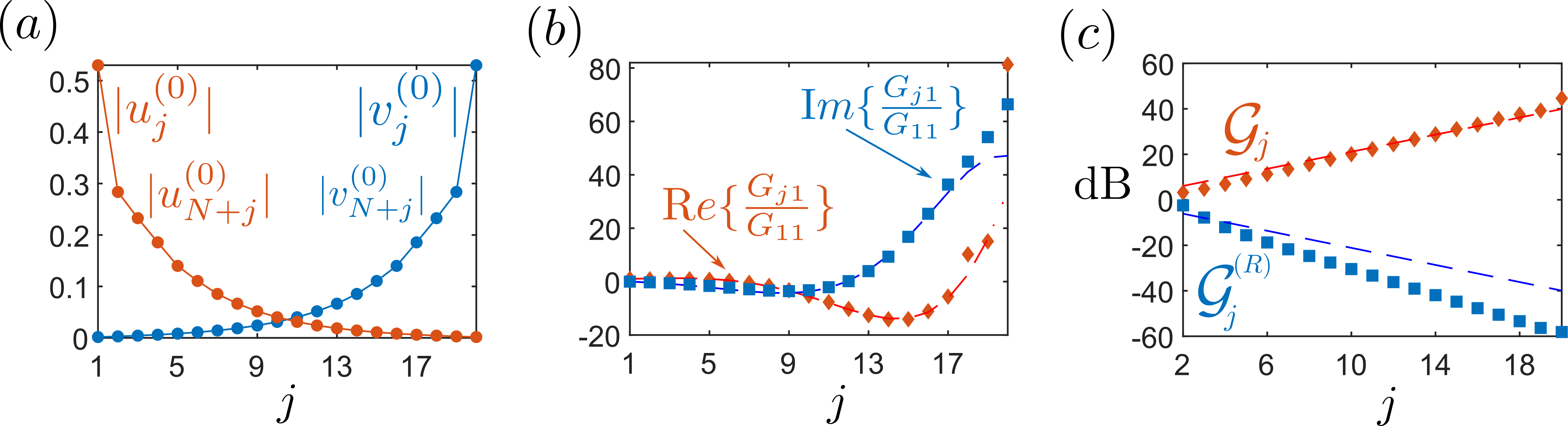
Figure 6: Connection between edge states of $\cal{H}(\omega)$ and exponential dependence of Green’s functions. (a) Absolute value of edge states $|u_{j}^{(0)}|$ and $|u_{N+j}^{(0)}|$ (red) and $|v_{j}^{(0)}|$ and $|v_{N+j}^{(0)}|$ (blue) as function of array site $j$ and for given $\omega=-0.5J$. (b) Real part (red diamonds) and imaginary part (blue squares) of the normalized Green‘s function $G_{j1}/G_{11}$ as a function of site index $j$. Dashed lines correspond to the exponential fit $G_{j1}/G_{11}=e^{\zeta(j-1)}$ with a localization length $\zeta\approx 0.22-0.29i$. (c) Exponential dependence of gain $G_{j}$ and reverse gain $G_{j}^{(R)}$. Dashed lines correspond to the prediction from the exponential fit in (b). Notice that the fit works well for the gain, but it overestimates the reverse gain (see text). We consider parameter set $P_{1}$ with $N=20$ and $\omega=-0.5J$, as used in Fig. 2.

Appendix D Directional amplification from edge states of extended Hamiltonian

In this appendix, we give details on the fundamental relation between the edge states of the extended Hamiltonian ${\cal H}(\omega)$ in Eq. (7) and the topological amplification properties of the system, such as the exponential dependence of the Green’s functions. A more extended description of this theoretical framework can be found in our previous work [27].

The starting point of our formalism is the expression of the Green’s function matrix $G(\omega)=(\omega-H_{\rm nh})^{-1}$ by means of of the following singular value decomposition (SVD):

$$\omega-H_{\rm nh}=U(\omega)S(\omega)V^{\dagger}(\omega).$$ (36)

Here, $U(\omega)$, $V(\omega)$, are unitary matrices and $S(\omega)$ is a semi-positive diagonal matrix, $S(\omega)_{nm}=\delta_{nm}E_{n}(\omega)$. Using this decomposition we can write,

$$G(\omega) =V(\omega)S^{-1}(\omega)U^{\dagger}(\omega)$$

$$=\sum_{n}E_{n}^{-1}(\omega)\vec{v}^{(n)}(\omega)\vec{u}^{(n)}{}^{\dagger}(\omega),$$ (37)

where $E_{n}(\omega)\geq 0$ are singular values, whereas $\vec{u}^{(n)}(\omega)$ and $\vec{v}^{(n)}(\omega)$ are the associated singular vectors given by the columns of $U(\omega)$ and $V(\omega)$, respectively. As originally demonstrated in Ref. [25], the quantities $E_{n}(\omega)$, $\vec{v}^{(n)}(\omega)$, and $\vec{u}^{(n)}(\omega)$ can also be interpreted as the positive eigenenergies and the associated eigenvectors of the extended Hamiltonian ${\cal H}(\omega)$ defined in Eq. (7). Therefore, the decomposition (37) can also be obtained by solving the eigenvalue problem

$${\cal H}(\omega)\begin{pmatrix}\vec{u}^{(n)}\\ \vec{v}^{(n)}\end{pmatrix}=\pm E_{n}\begin{pmatrix}\vec{u}^{(n)}\\ \pm\vec{v}^{(n)}\end{pmatrix}.$$ (38)

The extended Hamiltonian ${\cal H}(\omega)$ has an intrinsic chiral symmetry which may induce to the emergence of zero-energy modes in the spectrum $E_{n}$. A crucial observation is that those zero-energy modes lead to the enhancement of the Green’s function, since $E_{n}$ appears inverted in Eq. (37).

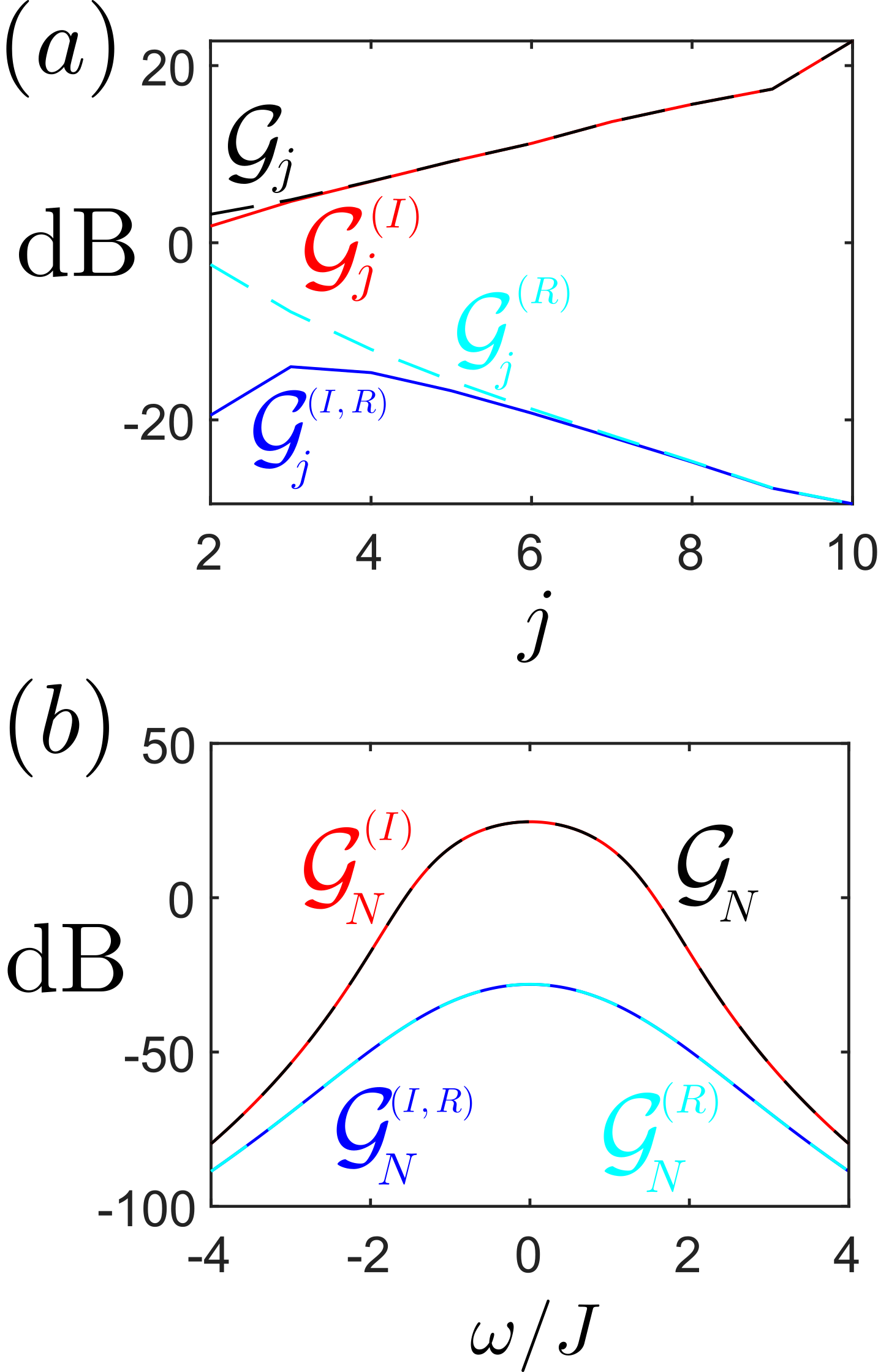
Figure 7: Comparison of gain and reverse gain for signal and idler fields. (a) Spatial dependence of signal gain ${\cal G}_{j}$ (black, dashed), idler gain ${\cal G}_{j}^{(I)}$ (red, dashed), signal reverse gain ${\cal G}^{(R)}_{j}$ (cyan, dashed), and idler reverse gain ${\cal G}_{j}^{(I,R)}$ (blue, solid) as function of array index $j$, for given frequency $\omega_{s}=-0.5J$. (b) Frequency dependence of the same quantities, evaluated at the last site $j=N$. Parameters are for operation point $P_{1}^{\prime}$ with $N=10$.

	$N$	$M$	$N_{JJ}$	$g_{c}/J$	$\kappa/J$	$C_{a}$	$C_{a}^{\prime}$	$ME_{J}/h$	$C_{aw}$	$C_{a}^{\rm eq}$	$L_{a}^{\rm eq}$	$C_{ab}$	$C_{b}$	$E_{C}/h$	$K_{c}/2\pi$	$J_{a}/2\pi$	$\kappa/2\pi$	$P_{b}$	$|\alpha|^{2}$	$J/2\pi$
						(fF)	(fF)	(THz)	(fF)	(fF)	(pH)	(fF)	(fF)	(MHz)	(kHz)	(MHz)	(MHz)	(dBm)		(MHz)
$P_{1}$	8	1	17	0.6	2.6	1790	1020	1.00	386	4220	81.7	6.26	388	4.57	2290	-31.2	406	-74.8	41.0	156
$P_{1}^{\prime}$	10	7	147	0.6	2.6	76.2	89.3	0.623	113	368	921	1.85	392	52.4	535	-31.2	406	-68.5	175	156
$P_{2}$	27	32	1760	0.25	0.9	48.6	108	2.85	103	368	921	1.85	392	52.4	25.6	187	337	-55.8	3660	375
$P_{3}$	4	22	198	0.95	2.8	106	84.4	1.96	93.5	368	921	1.85	392	52.4	54.1	-88.7	276	-59.5	1730	98.6

Table 1: Circuit parameters for various operation points of the topological JTWPA. The first five columns show general quantities that describe each operation point $P_{1}$, $P_{1}^{\prime}$, $P_{2}$, and $P_{3}$, of the amplifier, namely the number of sites $N$ of the JJ array, number of JJs $M$ on each sub-array, total number of JJs $N_{JJ}$ in the device, ratio between non-local parametric drive and hopping $g_{c}/J$, ratio between local decay and hopping $\kappa/J$. The next eight columns show specific circuit parameters of the JJ and auxiliary arrays, such as on-site capacitance $C_{a}$, inter-site capacitance $C_{a}^{\prime}$, Josephson frequency of each on-site JJ $ME_{J}/h$ (inter-site Josephson frequency is always half), capacitance $C_{aw}$ of the coupling to the input/output ports, equivalent (total) on-site capacitance $C_{a}^{\rm eq}$, equivalent on-site inductance $L_{a}^{\rm eq}$, coupling capacitance $C_{ab}$ between auxiliary and JJ array, and on-site capacitance of the auxiliary array $C_{b}$ (all other parameters of the auxiliary array are fixed and shown in the text). The next four columns show effective properties of the JJ array such charging frequency $E_{C}/h$, cross-Kerr nonlinearity $K_{c}$ (self-Kerr is always twice), linear hopping $J_{a}$, and effective decay rate $\kappa$ for coupling the input/output ports. The last three columns show the power $P_{b}$ of the pump on the auxiliary array, the mean number of photons $|\alpha|^{2}$ that this pump induces on the JJ array, and the effective inter-site hopping $J=J_{a}+2K_{c}|\alpha|^{2}$ which ultimately determines the bandwidth of the topological JTWPA.

Following the reasoning above, the characterization of the spectral amplifying properties of the system can be obtained by exploiting the relation between the Green’s function and the eigenstates of the effective Hamiltonian In particular, we can identify topological amplification regimes in which the extended Hamiltonian ${\cal H}(\omega)$ is in a topologically non-trivial phase according to the ten-fold way [38]. In that case, the eigen-spectrum $E_{n}$ presents at least one pair of zero-energy modes $\pm E_{0}$ with exponentially small energy, $E_{0}\propto e^{-N\zeta}$. Also, the associated zero-energy eigenvectors behave as edge states localized either on the right boundary, $v^{(0)}_{j}\sim v^{(0)}_{N+j}\sim e^{j\zeta}$, or on the left boundary, $u^{(0)}_{j}\sim u^{(0)}_{N+j}\sim e^{-j\zeta}$, with $\zeta$ the inverse localization length. In Fig. 6(a) we present a numerical check of the existence of those localized singular vectors for the same parameters used in Fig. 2. Note that for these parameters, we have the condition $u_{N+j}^{(0)}=iu_{j}^{(0)}$ and $v_{j,N+l}^{(0)}=iv_{j}^{(0)}$ and therefore they overlap in Fig. 6(a).

The exponential suppression with system size of the energy of zero-energy eigenvectors suggests that the first term of the SVD decomposition is the dominant contribution to the Green’s function,

$$G_{jl}(\omega)={} E_{0}^{-1}(\omega)v^{(0)}_{j}(\omega)u^{(0)}_{l}{}^{\ast}(\omega)$$

$$+\sum_{n>0}E_{n}^{-1}(\omega)v^{(n)}_{j}(\omega)u^{(n)}_{l}{}^{\ast}(\omega).$$ (39)

Indeed, for $j>l$, the first term in the right-hand side of Eq. (39) is exponentially larger than the contributions with $n\neq 0$, and therefore the Green’s function $G_{jl}(\omega)$ can be well-approximated as stated in the main text, by

$$G_{jl}(\omega)\approx e^{(j-l)\zeta(\omega)}G_{11}(\omega),\qquad j>l.$$ (40)

This occurs analogously for the anomalous components $G_{j,N+l}(\omega)$ when $j>l$. In Fig. 6(b) we numerically confirm this approximation by performing an exponential fit to the real and imaginary parts of the normalized Green’s function components $G_{j1}/G_{11}$, numerically calculated with the expression $G_{jl}=(\omega-H_{\rm nh})^{-1}_{jl}$. We see that the fit $G_{j1}/G_{11}=e^{\zeta(j-1)}$ with $\zeta\approx 0.22-0.29i$ agrees very well with the numerical data, up to finite size effects near the boundary $j=N$ [cf. dashed lines in Fig. 6(b)]. Note that using the decimation technique, the inverse localization length and the exponential dependence of Green’s functions can be analytically demonstrated [39, 52].

The exponential dependence of $G_{j1}(\omega)$ also implies that the topological amplifier’s gain grows exponentially ${\cal G}_{j}=\kappa^{2}|G_{j1}(\omega)|^{2}\sim e^{2\zeta(j-1)}|G_{11}(\omega)|^{2}$. In Fig. 6(c) we show that the gain grows exponentially very close to the theoretical prediction [cf. red diamonds and dashed line in Fig. 6(c)].

Note, however, that in our numerical calculations [cf. blue squares and dashed line in Fig. 6(c)], the reverse gain ${\cal G}_{j}^{(R)}$ turns out to be even lower than the decreasing exponential scaling $\propto e^{-2\zeta(j-1)}$ that one would naively expect. The reason for this lies in the decomposition (39). For $j<l$, the first term $\sim E_{0}^{-1}$ shows indeed the exponential dependence $\sim e^{-\zeta|j-l|}$, but this exponentially suppressed term does not dominate the behavior of $G_{jl}$, as it is on the same order as the sum of all the others. We have found numerically that, remarkably, contributions from singular vectors with $n\neq 0$ interfere destructively with each other, resulting in a reverse gain that is even more suppressed than one can expect from the exponential dependence of the edge states alone [cf. Fig. 6(c)]. Therefore, increasing the array size $N$ is doubly beneficial since it enhances exponentially both directional amplification and suppression of backward emission.

Finally, we comment that the behavior for the idler field at frequency $\omega=-\omega_{s}$ is qualitatively equal to what is shown in the main text for the signal field at $\omega=\omega_{s}$. In particular, when $\Delta=0$, we see that $G_{j,N+l}=iG_{jl}$ and therefore ${\cal G}_{j}$ and ${\cal G}_{j}^{(R)}$ are equivalent to ${\cal G}_{j}^{(I)}$ and ${\cal G}_{j}^{(R,I)}$, up to finite size effects at the boundaries. We present a numerical check of this result in Fig. 7(a)-(b), where we show the spatial and frequency dependence of all these quantities for the same parameters as Fig. 2.

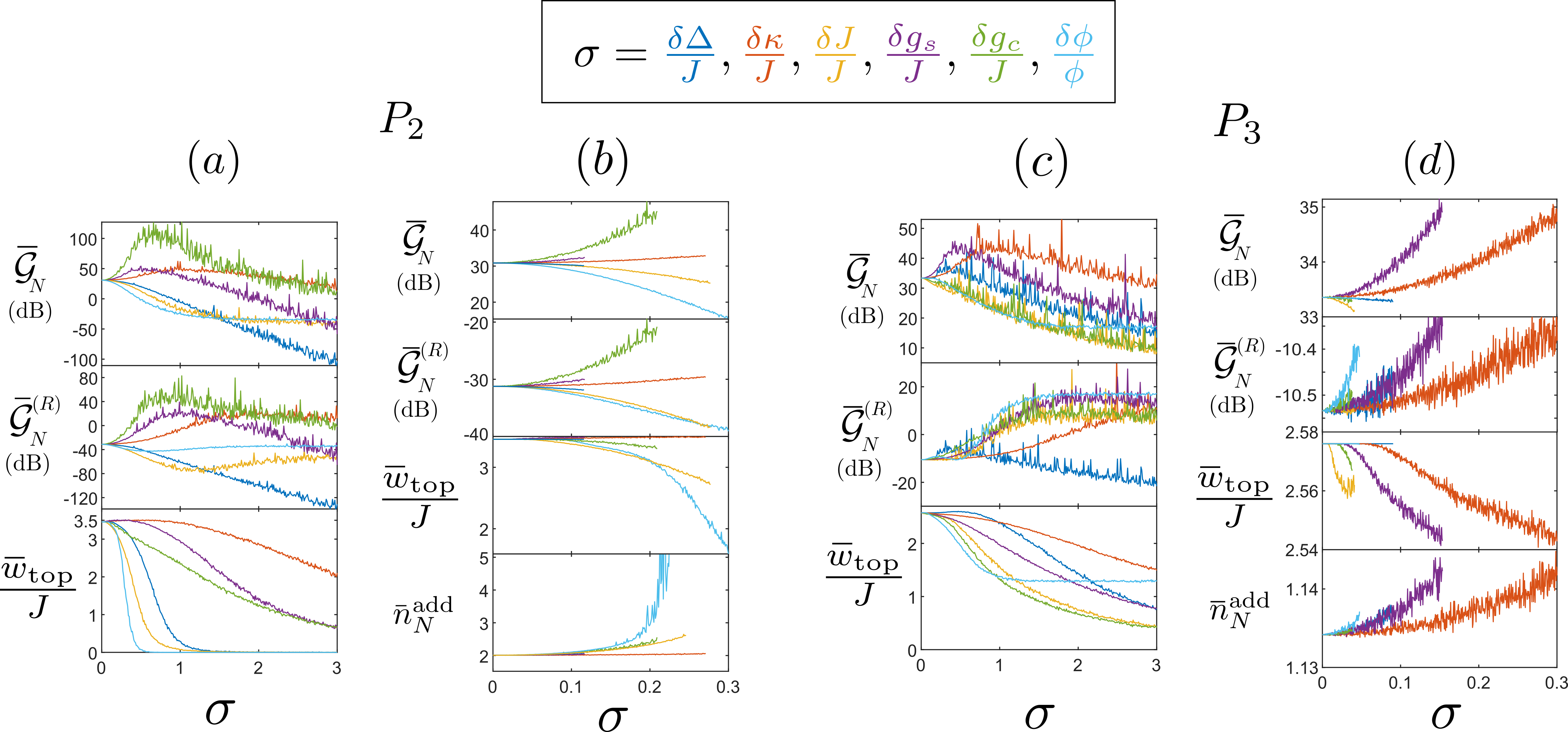
Figure 8: Robustness to disorder for operation points $P_{2}$ and $P_{3}$. (a)-(b) Average gain $\bar{{\cal G}}_{N}$, reverse gain $\bar{{\cal G}}_{N}^{(R)}$, topological bandwidth $\bar{w}_{\rm top}/J$, and added noise $\bar{n}_{\rm add}^{N}$ as function of the dimensionless disorder strength $\sigma$, defined for each effective system parameter as $\sigma=\delta\Delta/J$ (blue), $\sigma=\delta\kappa/J$ (red), $\sigma=\delta J/J$ (yellow), $\sigma=\delta g_{s}/J$ (purple), $\sigma=\delta g_{c}/J$ (green), and $\sigma=\delta\phi/\phi$ (cyan). All quantities are averaged over 1000 realizations for each type of disorder around the mean values defined by parameters $P_{2}$. Panel (b) is a zoom of (a) for $\sigma\leq 0.3$ and the termination of certain curves indicate the disorder at which the steady-state becomes unstable. (c)-(d) show the same quantitis as (a)-(b), but for mean parameters $P_{3}$. The frequency of the input signal is set to $\omega_{s}=-0.5J$ in all cases.

Appendix E Experimental parameters

In our work, we analyze three operation points $P_{1}-P_{3}$ for the topological JTWPA [cf. Fig. 2(d)]. For $P_{1}$ we consider parameters similar to Ref. [34] such that the JJ array has a capacitance $C_{a}^{\rm eq}\sim 4.2$ pF, Josephson inductance $L_{a}^{\rm eq}\sim 0.082$ nH, and impedance $Z_{a}=4.4$ $\Omega$. For $P_{1}^{\prime}$, $P_{2}$, and $P_{3}$, we consider parameters similar to Ref. [33] with $C_{a}^{\rm eq}\sim 0.37$ pF, $L_{a}^{\rm eq}\sim 1$ nH, and $Z_{a}=50$ $\Omega$. In all cases, the on-site frequency is fixed to $\omega_{a}/2\pi=8.56$ GHz, the non-local parametric drive $g_{c}/2\pi=93.7$ MHz, and the ratio $g_{s}/g_{c}=1$. This latter condition requires $K_{s}/K_{c}=2$ which is controlled by setting $E_{J}/E_{J}^{\prime}=2$. The strength of Kerr nonlinearities depends on $M$ and on the charging energy $E_{C}$. These and other effective quantities of the JJ array are indicated in Table 1 for each operation point.

Except for the capacitances $C_{ab}$ and $C_{b}$ shown in Table 1, all other parameters of the auxiliary array are fixed for all operation points to $L_{b}=0.995$ nH, $C_{b}^{\prime}=1.99$ fF, $C_{bw}=39.8$ fF, $L_{b}^{\rm eq}=398$ fF, $Z_{b}=50\Omega$, and $Z_{w}=50\Omega$. This leads to a frequency $\omega_{b}/2\pi=8.00$ GHz, intra-array hopping $J_{b}/2\pi=20$ MHz, intra-array hopping $J_{ab}/2\pi=20$MHz, and decay rate on the boundaries $\Gamma/2\pi=40$ MHz ($=2J_{b}$). Importantly, for these parameters, the effective detuning on the JJ array vanishes $\Delta=0$, the non-local decay on the JJ array $\kappa_{\rm nl}/2\pi=10$ MHz can be neglected compared to all other effective quantities, and the intra-array detuning $|\omega_{b}-\omega_{a}|/2\pi=560$ MHz is much larger than $J_{ab}$ and $J_{b}$, which leads to $\phi=\pi/2$. Note that we have neglected the intrinsic decay of auxiliary cavities provided they are smaller than $\kappa_{nl}$. Finally, the pump and signal powers, depend strongly on the operation point of the amplifier and its saturation properties. In particular, we consider $|\alpha_{s}|^{2}/2\pi\sim 5$ MHz for $P_{1}$, $P_{1}^{\prime}$, and $P_{3}$, whereas for $P_{2}$ we have $|\alpha_{s}|^{2}/2\pi\sim 19$MHz. The pump powers $P_{b}$ are chosen in the range between $-75$ to $-55$ dBm [cf. Table 1], which is standard in JTWPAs [15].

Appendix F Topological protection to disorder at operation points P2 and P3

The main features of the topological protection against disorder are discussed in Sec. V of the main text on the example of the operation point $P_{1}^{\prime}$ of the amplifier. The results are qualitatively similar for operation points $P_{2}$ and $P_{3}$, but there are some quantitative differences, especially regarding the stability, which we shortly address here.

The complete data is shown in Figs. 8(a)-(d). Here, for an input signal of frequency $\omega_{s}=-0.5J$, we display the average gain $\bar{{\cal G}}_{N}$, reverse gain $\bar{{\cal G}}^{(R)}_{N}$, topological bandwidth $\bar{w}_{\rm top}$, and added noise $\bar{n}_{N}^{\rm add}$ as a function of the dimensionless disorder strength for all effective system parameters defined as $\sigma=\delta\Delta/J$ (blue), $\sigma=\delta\kappa/J$ (red), $\sigma=\delta J/J$ (yellow), $\sigma=\delta g_{s}/J$ (purple), $\sigma=\delta g_{c}/J$ (green), and $\sigma=\delta\phi/\phi$ (cyan). Panels (a)-(b) correspond to the operation point $P_{2}$, while panels (c)-(d) correspond to $P_{3}$. In addition, panels (b) and (d) are a zoom of panels (a) and (c), respectively, where we show in more detail the behaviour of the average quantities for $\sigma\leq 0.3$. In these zoom panels (b) and (d) the ending of a curve before $\sigma=0.3$ indicates the disorder strength at which the steady-state becomes unstable (i.e. when the imaginary part of at least one eigenvalue of $H_{\rm nh}$ becomes positive).

First we discuss the operation point $P_{2}$ as it is the most similar to $P_{1}^{\prime}$: We see that disorder in $\delta g_{s}$ (purple), $\delta g_{c}$ (green), and $\delta J$ (red) increase the gain $\bar{{\cal G}}_{N}$ and reverse gain $\bar{{\cal G}}_{N}^{(R)}$ for $\sigma\leq 1$. This enhances the amplification but reduces the directionality. For $\sigma\gg 1$, all types of disorder destroy the topological properties of the amplification as they reduce gain, reverse gain, and topological bandwidth, while increasing added noise, analogously as what happens for $P_{1}^{\prime}$. The main difference in the behavior between operation points $P_{2}$ and $P_{1}^{\prime}$ is that at $P_{2}$ the amplifier becomes unstable at a slightly lower disorder due to the closer proximity to the instability region in Fig. 4. However, for both cases, the system is still robust up to a disorder strength $\sigma\lesssim 0.1$ in all system parameters, with minimum change in the overall amplifying performance, including a minimum increase in added noise.

In the case of the operation point $P_{3}$, the disorder in $\delta g_{s}$, $\delta\kappa$, and $\delta\Delta$ increase the gain for moderate disorder $\sigma\lesssim 1$, and then for $\sigma\gg 1$ all types of disorder reduce it. Interestingly, amplification is still maintained with up to 10 dB of gain for a large disorder of $\sigma\sim 3$. Nevertheless, such a large disorder destroys the directionality of the device by making the reverse gain positive (except for disorder in $\delta\Delta$). As for $P_{1}^{\prime}$ and $P_{2}$, the disorder in all parameters reduces topological bandwidth and increases added noise. It is curious to note that a large disorder in $\delta\phi$ does not reduce $\bar{w}_{\rm top}$ to zero, but it saturates at a finite value. In practice, however, this behavior is not possible to be observed since the system becomes unstable at a much lower disorder of $\delta\phi/\phi\sim 0.5$ for the case of phase. In general, the amplifier at the operation point $P_{3}$ is more unstable than at points $P_{1}^{\prime}$ and $P_{2}$ due to its proximity to the unstable region and also for having a larger inverse localization length ${\rm Re}[\zeta]\sim 1$. This makes the amplifier more susceptible to small changes in parameters. However, we see that the topological amplifier at this point is still robust to a disorder of order $3\%$ in all system parameters.

References

- Smith et al. [2013] D. M. P. Smith, L. Bakker, R. H. Witvers, B. E. M. Woestenburg, and K. D. Palmer, Low noise amplifier for radio astronomy, International Journal of Microwave and Wireless Technologies 5, 453 (2013).
- Cleland et al. [2002] A. N. Cleland, J. S. Aldridge, D. C. Driscoll, and A. C. Gossard, Nanomechanical displacement sensing using a quantum point contact, Appl. Phys. Lett. 81, 1699 (2002).
- Blais et al. [2021] A. Blais, A. L. Grimsmo, S. Girvin, and A. Wallraff, Circuit quantum electrodynamics, Rev. Mod. Phys. 93, 025005 (2021).
- García-Ripoll [2022] J. J. García-Ripoll, Quantum Information and Quantum Optics with Superconducting Circuits (Cambridge University Press, Cambridge, 2022).
- Vijay et al. [2011] R. Vijay, D. H. Slichter, and I. Siddiqi, Observation of Quantum Jumps in a Superconducting Artificial Atom, Phys. Rev. Lett. 106, 110502 (2011).
- Walter et al. [2017] T. Walter, P. Kurpiers, S. Gasparinetti, P. Magnard, A. Potočnik, Y. Salathé, M. Pechal, M. Mondal, M. Oppliger, C. Eichler, and A. Wallraff, Rapid High-Fidelity Single-Shot Dispersive Readout of Superconducting Qubits, Phys. Rev. Applied 7, 054020 (2017).
- Dassonneville et al. [2020] R. Dassonneville, T. Ramos, V. Milchakov, L. Planat, E. Dumur, F. Foroughi, J. Puertas, S. Leger, K. Bharadwaj, J. Delaforce, C. Naud, W. Hasch-Guichard, J. García-Ripoll, N. Roch, and O. Buisson, Fast High-Fidelity Quantum Nondemolition Qubit Readout via a Nonperturbative Cross-Kerr Coupling, Phys. Rev. X 10, 011045 (2020).
- Pereira et al. [2022] L. Pereira, J. J. García-Ripoll, and T. Ramos, Parallel QND measurement tomography of multi-qubit quantum devices, arXiv:2204.10336 (2022).
- Macklin et al. [2015] C. Macklin, K. O’Brien, D. Hover, M. E. Schwartz, V. Bolkhovsky, X. Zhang, W. D. Oliver, and I. Siddiqi, A near–quantum-limited Josephson traveling-wave parametric amplifier, Science 350, 307 (2015).
- White et al. [2015] T. C. White, J. Y. Mutus, I.-C. Hoi, R. Barends, B. Campbell, Y. Chen, Z. Chen, B. Chiaro, A. Dunsworth, E. Jeffrey, J. Kelly, A. Megrant, C. Neill, P. J. J. O’Malley, P. Roushan, D. Sank, A. Vainsencher, J. Wenner, S. Chaudhuri, J. Gao, and J. M. Martinis, Traveling wave parametric amplifier with Josephson junctions using minimal resonator phase matching, Appl. Phys. Lett. 106, 242601 (2015).
- Planat et al. [2020] L. Planat, A. Ranadive, R. Dassonneville, J. Puertas Martínez, S. Léger, C. Naud, O. Buisson, W. Hasch-Guichard, D. M. Basko, and N. Roch, Photonic-Crystal Josephson Traveling-Wave Parametric Amplifier, Phys. Rev. X 10, 021021 (2020).
- Winkel et al. [2020] P. Winkel, I. Takmakov, D. Rieger, L. Planat, W. Hasch-Guichard, L. Grünhaupt, N. Maleeva, F. Foroughi, F. Henriques, K. Borisov, J. Ferrero, A. V. Ustinov, W. Wernsdorfer, N. Roch, and I. M. Pop, Nondegenerate Parametric Amplifiers Based on Dispersion-Engineered Josephson-Junction Arrays, Phys. Rev. Applied 13, 024015 (2020).
- Eichler and Wallraff [2014] C. Eichler and A. Wallraff, Controlling the dynamic range of a Josephson parametric amplifier, EPJ Quantum Technol. 1, 2 (2014).
- Roy and Devoret [2016] A. Roy and M. Devoret, Introduction to parametric amplification of quantum signals with Josephson circuits, Comptes Rendus Physique Quantum microwaves / Micro-ondes quantiques, 17, 740 (2016).
- Esposito et al. [2021] M. Esposito, A. Ranadive, L. Planat, and N. Roch, Perspective on traveling wave microwave parametric amplifiers, Appl. Phys. Lett. 119, 120501 (2021).
- Abdo et al. [2013] B. Abdo, K. Sliwa, L. Frunzio, and M. Devoret, Directional Amplification with a Josephson Circuit, Phys. Rev. X 3, 031001 (2013).
- Sliwa et al. [2015] K. Sliwa, M. Hatridge, A. Narla, S. Shankar, L. Frunzio, R. Schoelkopf, and M. Devoret, Reconfigurable Josephson Circulator/Directional Amplifier, Phys. Rev. X 5, 041020 (2015).
- Metelmann and Clerk [2015] A. Metelmann and A. Clerk, Nonreciprocal Photon Transmission and Amplification via Reservoir Engineering, Phys. Rev. X 5, 021025 (2015).
- Lecocq et al. [2017] F. Lecocq, L. Ranzani, G. Peterson, K. Cicak, R. Simmonds, J. Teufel, and J. Aumentado, Nonreciprocal Microwave Signal Processing with a Field-Programmable Josephson Amplifier, Phys. Rev. Applied 7, 024028 (2017).
- Fang et al. [2017] K. Fang, J. Luo, A. Metelmann, M. H. Matheny, F. Marquardt, A. A. Clerk, and O. Painter, Generalized non-reciprocity in an optomechanical circuit via synthetic magnetism and reservoir engineering, Nature Phys 13, 465 (2017).
- Pucher et al. [2022] S. Pucher, C. Liedl, S. Jin, A. Rauschenbeutel, and P. Schneeweiss, Atomic spin-controlled non-reciprocal Raman amplification of fibre-guided light, Nat. Photon. 16, 380 (2022).
- Heinsoo et al. [2018] J. Heinsoo, C. K. Andersen, A. Remm, S. Krinner, T. Walter, Y. Salathé, S. Gasparinetti, J.-C. Besse, A. Potočnik, A. Wallraff, and C. Eichler, Rapid High-fidelity Multiplexed Readout of Superconducting Qubits, Phys. Rev. Applied 10, 034040 (2018).
- Ozawa et al. [2019] T. Ozawa, H. M. Price, A. Amo, N. Goldman, M. Hafezi, L. Lu, M. C. Rechtsman, D. Schuster, J. Simon, O. Zilberberg, and I. Carusotto, Topological photonics, Rev. Mod. Phys. 91, 015006 (2019).
- Peano et al. [2016] V. Peano, M. Houde, F. Marquardt, and A. A. Clerk, Topological Quantum Fluctuations and Traveling Wave Amplifiers, Phys. Rev. X 6, 041026 (2016).
- Porras and Fernández-Lorenzo [2019] D. Porras and S. Fernández-Lorenzo, Topological Amplification in Photonic Lattices, Phys. Rev. Lett. 122, 143901 (2019).
- Wanjura et al. [2020] C. C. Wanjura, M. Brunelli, and A. Nunnenkamp, Topological framework for directional amplification in driven-dissipative cavity arrays, Nature Communications 11, 3149 (2020).
- Ramos et al. [2021] T. Ramos, J. J. García-Ripoll, and D. Porras, Topological input-output theory for directional amplification, Phys. Rev. A 103, 033513 (2021).
- Koch et al. [2010] J. Koch, A. A. Houck, K. L. Hur, and S. M. Girvin, Time-reversal-symmetry breaking in circuit-qed-based photon lattices, Phys. Rev. A 82, 043811 (2010).
- Roushan et al. [2017] P. Roushan, C. Neill, A. Megrant, Y. Chen, R. Babbush, R. Barends, B. Campbell, Z. Chen, B. Chiaro, A. Dunsworth, A. Fowler, E. Jeffrey, J. Kelly, E. Lucero, J. Mutus, P. J. J. O’Malley, M. Neeley, C. Quintana, D. Sank, A. Vainsencher, J. Wenner, T. White, E. Kapit, H. Neven, and J. Martinis, Chiral ground-state currents of interacting photons in a synthetic magnetic field, Nature Physics 13, 146 (2017).
- Peng et al. [2022] K. Peng, M. Naghiloo, J. Wang, G. D. Cunningham, Y. Ye, and K. P. O’Brien, Floquet-mode traveling-wave parametric amplifiers, PRX Quantum 3, 020306 (2022).
- Carrasco et al. [2022] J. Carrasco, D. Valenzuela, C. Falcón, R. Finger, and F. P. Mena, The effect of complex dispersion and characteristic impedance on the gain of superconducting traveling-wave kinetic inductance parametric amplifiers, arXiv:2210.00626 (2022).
- Kreikebaum et al. [2020] J. M. Kreikebaum, K. P. O’Brien, A. Morvan, and I. Siddiqi, Improving wafer-scale Josephson junction resistance variation in superconducting quantum coherent circuits, Supercond. Sci. Technol. 33, 06LT02 (2020).
- Eichler et al. [2014] C. Eichler, Y. Salathe, J. Mlynek, S. Schmidt, and A. Wallraff, Quantum-Limited Amplification and Entanglement in Coupled Nonlinear Resonators, Phys. Rev. Lett. 113, 110502 (2014).
- Mutus et al. [2014] J. Y. Mutus, T. C. White, R. Barends, Y. Chen, Z. Chen, B. Chiaro, A. Dunsworth, E. Jeffrey, J. Kelly, A. Megrant, C. Neill, P. J. J. O’Malley, P. Roushan, D. Sank, A. Vainsencher, J. Wenner, K. M. Sundqvist, A. N. Cleland, and J. M. Martinis, Strong environmental coupling in a Josephson parametric amplifier, Appl. Phys. Lett. 104, 263513 (2014).
- Kounalakis et al. [2018] M. Kounalakis, C. Dickel, A. Bruno, N. K. Langford, and G. A. Steele, Tuneable hopping and nonlinear cross-Kerr interactions in a high-coherence superconducting circuit, npj Quantum Inf 4, 38 (2018).
- Ranadive et al. [2022] A. Ranadive, M. Esposito, L. Planat, E. Bonet, C. Naud, O. Buisson, W. Guichard, and N. Roch, Kerr reversal in Josephson meta-material and traveling wave parametric amplification, Nat Commun 13, 1737 (2022).
- Gómez-León et al. [2022] A. Gómez-León, T. Ramos, A. González-Tudela, and D. Porras, Bridging the gap between topological non-hermitian physics and open quantum systems, Phys. Rev. A 106, L011501 (2022).
- Ryu et al. [2010] S. Ryu, A. P. Schnyder, A. Furusaki, and A. W. W. Ludwig, Topological insulators and superconductors: tenfold way and dimensional hierarchy, New J. Phys. 12, 065010 (2010).
- Gómez-León et al. [2022] A. Gómez-León, T. Ramos, D. Porras, and A. González-Tudela, Decimation technique for open quantum systems: A case study with driven-dissipative bosonic chains, Phys. Rev. A 105, 052223 (2022).
- Note [1] Note that the idler field at frequency manifest this same directional amplifying properties (see Appendix D).
- Planat et al. [2019] L. Planat, R. Dassonneville, J. P. Martínez, F. Foroughi, O. Buisson, W. Hasch-Guichard, C. Naud, R. Vijay, K. Murch, and N. Roch, Understanding the Saturation Power of Josephson Parametric Amplifiers Made from SQUID Arrays, Phys. Rev. Applied 11, 034014 (2019).
- Note [2] Notice that in the original work by Caves [58], the quantum limit of minimum noise corresponds to due to a different convention in the definition of the noise power.
- Note [3] Using sub-arrays of JJs [13] does not modify the linear properties of the superconducting circuit, but reduces the Kerr-nonlinearities as . Since can be increased maximum by a factor , the effective quantities and are not modified.
- Wanjura et al. [2021] C. C. Wanjura, M. Brunelli, and A. Nunnenkamp, Correspondence between Non-Hermitian Topology and Directional Amplification in the Presence of Disorder, Phys. Rev. Lett. 127, 213601 (2021).
- Note [4] Due to finite size effects, does not vanish at the interface with the trivial region . In the thermodynamic limit , zero energy modes become exact and the gap vanishes exactly at the boundary.
- Stützer et al. [2018] S. Stützer, Y. Plotnik, Y. Lumer, P. Titum, N. H. Lindner, M. Segev, M. C. Rechtsman, and A. Szameit, Photonic topological Anderson insulators, Nature 560, 461 (2018).
- Grimsmo et al. [2021] A. L. Grimsmo, B. Royer, J. M. Kreikebaum, Y. Ye, K. O’Brien, I. Siddiqi, and A. Blais, Quantum Metamaterial for Broadband Detection of Single Microwave Photons, Phys. Rev. Applied 15, 034074 (2021).
- Remm et al. [2022] A. Remm, S. Krinner, N. Lacroix, C. Hellings, F. Swiadek, G. Norris, C. Eichler, and A. Wallraff, Intermodulation Distortion in a Josephson Traveling Wave Parametric Amplifier, arXiv:2210.04799 (2022).
- Guimond et al. [2020] P.-O. Guimond, B. Vermersch, M. L. Juan, A. Sharafiev, G. Kirchmair, and P. Zoller, A unidirectional on-chip photonic interface for superconducting circuits, npj Quantum Information 6, 1 (2020).
- Flynn et al. [2021] V. P. Flynn, E. Cobanera, and L. Viola, Topology by dissipation: Majorana bosons in metastable quadratic markovian dynamics, Phys. Rev. Lett. 127, 245701 (2021).
- Kawabata et al. [2019] K. Kawabata, K. Shiozaki, M. Ueda, and M. Sato, Symmetry and topology in non-hermitian physics, Phys. Rev. X 9, 041015 (2019).
- Gómez-León et al. [2022] A. Gómez-León, T. Ramos, A. González-Tudela, and D. Porras, Non-hermitian topological phases in traveling-wave parametric amplifiers, arXiv:2207.13715 (2022).
- McDonald et al. [2022] A. McDonald, R. Hanai, and A. A. Clerk, Nonequilibrium stationary states of quantum non-hermitian lattice models, Phys. Rev. B 105, 064302 (2022).
- Tangpanitanon et al. [2016] J. Tangpanitanon, V. M. Bastidas, S. Al-Assam, P. Roushan, D. Jaksch, and D. G. Angelakis, Topological Pumping of Photons in Nonlinear Resonator Arrays, Phys. Rev. Lett. 117, 213603 (2016).
- Hafezi et al. [2013] M. Hafezi, M. D. Lukin, and J. M. Taylor, Non-equilibrium fractional quantum Hall state of light, New J. Phys. 15, 063001 (2013).
- Jin et al. [2013] J. Jin, D. Rossini, R. Fazio, M. Leib, and M. J. Hartmann, Photon Solid Phases in Driven Arrays of Nonlinearly Coupled Cavities, Phys. Rev. Lett. 110, 163605 (2013).
- Ramos et al. [2016] T. Ramos, B. Vermersch, P. Hauke, H. Pichler, and P. Zoller, Non-Markovian dynamics in chiral quantum networks with spins and photons, Phys. Rev. A 93, 062104 (2016).
- Caves [1982] C. M. Caves, Quantum limits on noise in linear amplifiers, Phys. Rev. D 26, 1817 (1982).