Effective and asymptotic criticality of structurally disordered magnets

Abstract

Changes in magnetic critical behaviour of quenched structurally-disordered magnets are usually exemplified in experiments and in MC simulations by diluted systems consisting of magnetic and non-magnetic components. By our study we aim to show, that similar effects can be observed not only for diluted magnets with non-magnetic impurities, but may be implemented, e.g., by presence of two (and more) chemically different magnetic components as well. To this end, we consider a model of the structurally-disordered quenched magnet where all lattice sites are occupied by Ising-like spins of different length $L$. In such random spin length Ising model the length $L$ of each spin is a random variable governed by the distribution function $p(L)$. We show that this model belongs to the universality class of the site-diluted Ising model. This proves that both models are described by the same values of asymptotic critical exponents. However, their effective critical behaviour differs. As a case study we consider a quenched mixture of two different magnets, with values of elementary magnetic moments $L_{1}=1$ and $L_{2}=s$, and of concentration $c$ and $1-c$, correspondingly. We apply field-theoretical renormalization group approach to analyze the renormalization group flow for different initial conditions, triggered by $s$ and $c$, and to calculate effective critical exponents further away from the fixed points of the renormalization group transformation. We show how the effective exponents are governed by difference in properties of the magnetic components.

1 Introduction

Beneath the most intriguing questions of modern condensed matter physics one should certainly name a problem of influence of structural disorder on criticality [1, 2, 3, 4, 5, 6]. Taken that a regular lattice (‘ideal’) magnet manifests a second order phase transition into magnetically-ordered state and a critical behaviour governed by some scaling laws, will these universal laws be altered by structural disorder induced into the system? Although this question addresses properties of matter in a narrow region of a phase diagram in the vicinity of a phase transition point, the answer on it is of a great importance both from the fundamental reasons (description of criticality arising in different systems ranging from high-energy physics to cosmogony) [1] as well as due to applications of structurally-disordered materials in modern technologies [7].

In the context of this paper we concentrate on the case, when the disorder in structure is implemented via quenched random local transition temperature [8]. An archetypal example is given by diluted uniaxial magnets Fe_xZn_1-xF₂, Mn_xZn_1-xF₂ obtained as a crystalline mixture of two compounds when a corresponding diluted alloy is prepared by a substitution of a non-magnetic isomorph ZnF₂ for its antiferromagnetic counterpart (FeF₂ or MnF₂) [9, 10, 11]. Relaxation times of such systems are much larger than typical observation times which allows one to perform their theoretical and numerical analysis in terms of quenched diluted random-site Ising model, Fig. 1b, see e.g., Refs. [4] and [12] for more recent references. Experimental data about critical behaviour of quenched diluted Heisenberg magnets has been reviewed in Refs. [13, 14, 15], and more recently in Refs. [16, 17, 18, 19].

For such systems, it is well established by now that even a weak structural disorder can modify their critical behaviour. The qualitative answer about the changes in the universality class of the 2nd order phase transition into magnetically ordered state is given by the heuristic Harris criterion [20]. It predicts that if the heat-capacity critical exponent $\alpha_{\rm pure}$ of the pure system is positive, i.e., the heat capacity diverges at the critical point, then a quenched disorder (e.g., dilution) causes changes in the universality class. In particular, values of universal critical exponents change. Consecutively, if $\alpha_{\rm pure}<0$ the universality class is the same as for the homogeneous system. In $d=3$ dimensions, it puts uniaxial magnets on a special place. Indeed, only for Ising-like magnets with a scalar (i.e., $m=1$-component) order parameter the heat capacity diverges at the critical point, $\alpha_{\rm pure}(m=1)>0$, whereas it does not diverge for the easy plane (XY) and Heisenberg magnets, $\alpha_{\rm pure}(m=2),\alpha_{\rm pure}(m=3)<0$, correspondingly, see Table 1. Numerous theoretical, experimental and numerical studies confirmed this observation and, in particular, lead to determination of accurate values of the asymptotic critical exponents of the 3d random Ising magnets in the new universality class [4, 12]. In Table 1 we list values of the critical exponents $\nu$, $\alpha$, and $\gamma$ for the correlation length, magnetic susceptibility and heat capacity of pure and quenched diluted 3d Ising model as obtained by resummation of the perturbative field-theoretical renormalization group expansions. There, we also give the values of the exponents for pure 3d XY and Heisenberg models.

Model	$\nu$	$\alpha$	$\gamma$
$m=1$ [21]	$0.6304(13)$	$0.109(4)$	$1.2396(13)$
$m=2$ [21]	$0.6703(15)$	$-0.011(4)$	$1.3169(20)$
$m=3$ [21]	$0.7073(35)$	$-0.122(10)$	$1.389(50)$
$m=1$, diluted [22]	$0.678(10)$	$-0.034(30)$	$1.336(20)$

Table 1: Asymtotic critical exponents of pure and quenched diluted 3d Ising model ($m=1$) as well as of the XY ($m=2$) and Heisenberg ($m=3$) models as obtained by resummation of the perturbative field-theoretical renormalization group expansions.

The above results concern values of the asymptotic exponents. By definition, an asymptotic exponent $x$ governs singular behaviour of the observable ${\cal O}$ directly at the critical point $T_{c}$:

$$x\equiv-\lim_{\tau\to 0}\frac{\ln{\cal O}(\tau)}{\ln\tau},\hskip 30.00005pt\tau=|T-T_{c}|/T_{c}\,.$$ (1)

However, an approach to $T_{c}$ is characterized by non-universal effective critical exponents, which are introduced to describe the behavior of a quantity in a certain temperature interval [23, 24]. These are defined as:

$$x_{\rm eff}(\tau)\equiv-\frac{\ln{\cal O}(\tau)}{\ln\tau}\,.$$ (2)

They are non-universal, change values with distance to the critical point and coincide with the asymptotic critical exponents only at (or close to) the critical point. For structurally disordered systems, an effective critical behaviour is especially rich and together with temperature distance to the critical point may be governed by such parameters as inhomogeneities concentration, their distribution, etc. Needless to say, that the effective non-universal critical behaviour of structurally-disordered magnets does not obey Harris criterion in a sense that the dilution modifies effective critical exponents irrespective of the divergence in the heat capacity of the corresponding pure magnet. In particular, numerous variations in scaling exponents of Heisenberg-like diluted magnets have been observed experimentally and interpreted as being effective exponents, not yet in an asymptotic regime. This concerns scaling of isothermal susceptibility [25, 26, 27, 28], spontaneous magnetisation [26, 27, 28], magnetocaloric coefficient [29], etc. The same is true for the diluted uniaxial Ising-like magnets: although the theory predicts changes in their universality class and hence new values of the asymptotic exponents (see Table 1), an effective exponents found in experiments may differ essentially [30].

From the theoretical perspective, there are attempts of qualitative prediction and quantitative description of the effective critical behavior for weakly diluted quenched Ising- [31, 32, 33] and Heisenberg-like [15, 33] magnets within the field-theoretical renormalization group (RG) picture. On the one hand, this method is capable to reproduce accurate values of the asymptotic exponents, on the other hand, it can also take into account possible violations of universality further away from the critical point. This is achieved by calculation of the RG functions further away from the fixed points of the RG transformation. In this way, the RG flow equations mimic approach to criticality whereas different initial conditions correspond to different non-universal factors, inherent to any specific magnet.

Our present paper continues aforementioned studies of effective critical behaviour of structurally disordered magnets, however it also serves as an attempt to look on the phenomenon from a different perspective. Indeed, the most common examples of structurally-disordered magnets with weak random-$T_{c}$-like disorder that were considered so far in experiments and in MC simulations are exemplified by diluted systems consisting of magnetic and non-magnetic components. In turn, changes in the critical exponents of structurally-disordered magnets are often attributed merely to the presence of a non-magnetic component. By our study we aim to show, that a similar effect may be observed not only for diluted magnets with non-magnetic impurities, but it is rather caused by presence of a quenched structural disorder which may be implemented, e.g., by presence of two (and more) chemically different magnetic components as well. To put it in a different way, we aim to show that this is the structural disorder itself that causes changes in the critical behaviour, whenever it has a form of randomly distributed quenched magnetic and non-magnetic constituents or the form of random mixture of two different magnetic compounds.

The rest of the paper is organized as follows. In the next section 2 we describe the random spin length Ising model and sketch the derivation of its effective Hamiltonian. In section 3 we consider particular cases of this model. We show that the effective Hamiltonian of the Ising model with randomly distributed elementary spins of two different lengths has the same symmetry as that of the site-diluted Ising model containing magnetic and non-magnetic sites. This proves that both systems belong to the same universality class and hence are described by the same values of asymptotic critical exponents. Moreover, we get the ratio of bare couplings of both effective Hamiltonians. This allows, in particular, to discriminate between different effective critical behaviours generated by both Hamiltonians. The last is analysed in details in Section 4. There, we apply the field-theoretical RG approach to analyze the RG flow for different initial conditions and to calculate effective critical exponents further away from the fixed points of the RG transformation. Doing so we also discuss possible differences in effective critical behaviour of two models under consideration. Conclusions and outlook are summarized in Section 5.

2 Functional representation for the free energy of the random spin length Ising model

In this chapter we introduce a model of structurally disordered magnet that will be analysed henceforth. Doing so we will get a functional representation of its free energy and define corresponding effective Hamiltonian. The last is a key object of analysis in the RG framework [34, 35]. Systems of different microscopic origin that are described in the critical region by the same effective Hamiltonian share the same universal features of critical behaviour: it is said that they belong to the same universality class.

It is convenient first to sketch a derivation of the effective Hamiltonian for the usual Ising model and to use this derivation further as a blueprint to elaborate effective Hamiltonians incorporating structural disorder. Let us consider a system of $N$ Ising spins $S_{\bf R}=\pm 1$ located on ${\bf R}$ sites of a $d$ dimensional hypercubic lattice that interact with the Hamiltonian:

$${\cal H}=-\frac{1}{2}\sum_{{\bf R},{\bf R}^{\prime}}J(|{\bf R}-{\bf R}^{\prime}|)S_{\bf R}S_{{\bf R}^{\prime}}\,.$$ (3)

Here and below sums (products) over ${\bf R}$ span all lattice sites. In the case of the Ising model, the interaction $J(R)>0$ is reduced to the nearest neighbours, but generally speaking one may consider any ferromagnetic short-range coupling. Symbolically, the model is depicted in Fig. 1a.

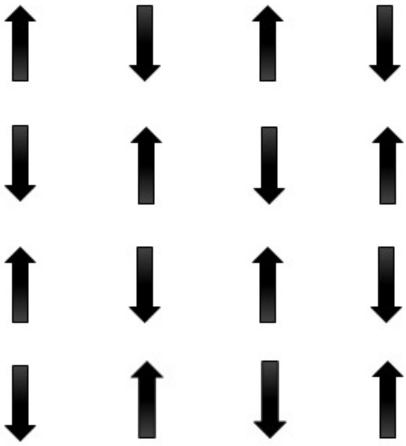
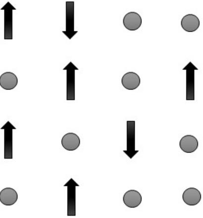
(a)                                                                             (b)

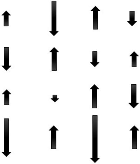
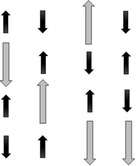
(c)                                                                             (d)

Figure 1: Lattice spin models discussed in this paper. (a) Ising model: magnetic atoms are described by pointing up and down ‘spins’ $S=\pm 1$ of equal length located on sites of a $d$-dimensional lattice. (b) Quenched diluted Ising model: a part of sites in model (a) are occupied by non-magnetic atoms (or are empty). Magnetic and non-magnetic sites are randomly distributed and fixed in a given positions. Only magnetic atoms interact. (c) Random spin length Ising model: the length $L$ of a spin in model (a) is a random variable governed by the distribution function $p(L)$, hence $S=\pm L$. (d) A particular case of model (c) when the distribution function is given by Eq. (27). Note that model (b) can be also considered as a particular case of (c) with the distribution function given by Eq. (24).

Thermodynamics of the model can be analysed given its free energy

$$F=-\beta^{-1}\ln Z\,$$ (4)

where $\beta=k_{\mathrm{B}}T$, $k_{\mathrm{B}}$ is the Boltzmann constant and the partition function reads

$$Z={\rm Sp}\,{\rm e}^{-\beta{\cal H}},\hskip 20.00003pt{\rm Sp}\,(\dots)=\prod_{\bf{R}}\sum_{S_{\bf{R}}=\pm 1}\,(\dots)\,.$$ (5)

One way to take trace in Eq. (5) is to represent the partition function in a form of the functional integral to get rid of the product of two spins in the Hamiltonian (3). This can be achieved, e.g., by applying the Stratonovich-Hubbard transformation. To this end, making use of the translational invariance of the Hamiltonian (5) one writes the partition function in the Fourier-space as a diagonal form:

$$Z={\rm Sp}\,\prod_{{\bf k}}e^{\frac{\beta\nu(k)}{2}{S}_{{\bf k}}{S}_{-{\bf k}}}\,,$$ (6)

here and below the wave vector ${\bf k}$ changes in the upper half of the corresponding Brillouin zone and $\nu(k)$, ${S}_{{\bf k}}$ are the Fourier images of the interaction and spins:

$$J(R)=\frac{1}{N}\sum_{{\bf k}}e^{i{\bf k}{\bf R}}\nu(k)\,,\hskip 20.00003pt\nu(k)=\sum_{{\bf R}}e^{-i{\bf k}{\bf R}}J(R)\,,$$ (7)

$$S_{\bf R}=\frac{1}{\sqrt{N}}\sum_{{\bf k}}e^{i{\bf k}{\bf R}}{S}_{{\bf k}}\,,\hskip 20.00003pt{S}_{{\bf k}}=\frac{1}{\sqrt{N}}\sum_{{\bf R}}e^{-i{\bf k}{\bf R}}S_{\bf R}\,.$$ (8)

For the exponent in Eq. (6), the Stratonovich-Hubbard transformation is defined via the integral identity:

$$e^{\frac{\beta\nu(k)}{2}{S}_{{\bf k}}{S}_{-{\bf k}}}=\sqrt{\frac{1}{2\pi\beta\nu(k)}}\int_{-\infty}^{\infty}{\rm d}{\phi}_{{\bf k}}e^{-\frac{{\phi}_{{\bf k}}{\phi}_{-{\bf k}}}{2\beta\nu(k)}+{S}_{{\bf k}}{\phi}_{-{\bf k}}}\,,\hskip 20.00003pt{\rm Re}\,\nu(k)>0\,,$$ (9)

with the functional integral over field ${\phi}_{{\bf k}}$ in the r.h.s. This transformation allows to reconsider a system of spins $S_{\bf R}$ interacting via the two-body potentials $J(R)$ as a system of independent particles interacting with a fluctuating field ${\phi}_{{\bf k}}$. Further steps of representing partition function of the $d$-dimensional Ising model in the form of a functional integral can be sketched as:

$$Z\sim\int({\rm d}{\phi}){\rm e}^{-\sum_{\bf k}\frac{1}{2\beta\nu(k)}{\phi}_{{\bf k}}{\phi}_{{\bf-k}}}{\rm Sp}\ {\rm e}^{\sum_{\bf R}{S}_{{\bf R}}{\phi}_{{\bf R}}}\sim\int({\rm d}{\phi}){\rm e}^{-\sum_{\bf k}\frac{1}{2\beta\nu(k)}{\phi}_{{\bf k}}{\phi}_{{\bf-k}}}\prod_{\bf R}\cosh({\phi}_{{\bf R}})\sim\,\int({\rm d}{\phi}){\rm e}^{-{\cal H}_{\rm eff}}\,.$$ (10)

Here and below we omit prefactors irrelevant for the subsequent analysis, ${\phi}_{\bf{R}}$ is the Fourier image of ${\phi}_{{\bf k}}$ and the functional integration means:

$$\int({\rm d}{\phi})=\prod_{\bf{R}}\int_{-\infty}^{\infty}{\rm d}{\phi}_{\bf{R}}\,.$$ (11)

Since the first expression in Eq. (10) contains only a linear in ${S}_{{\bf R}}$ term, the trace merely reduces to substituting there the value ${S}_{{\bf R}}=\pm 1$ and leads to the product of $\cosh({\phi}_{{\bf R}})$ in the second expression. In turn, in the critical region this function is approximated by an expansion up to the fourth order terms leading to the following effective Hamiltonian:

$${\cal H}_{\rm eff}=\frac{1}{2}\sum_{\bf k}\big{(}\frac{1}{\beta\nu(k)}-u_{2}\big{)}{\phi}_{{\bf k}}{\phi}_{{\bf-k}}+\frac{u_{4}}{4!}\sum_{\bf R}\phi_{\bf R}^{4}\,.$$ (12)

Coefficients $u_{2l}$ readily follow from the expansion of $\ln\cosh(x)$ in Eq. (10): $u_{2}/2=1/2$, $u_{4}/4!=1/12$. In the RG analysis of critical behaviour the short wave-length (small $k$) contributions to $\nu(k)$ are considered, the Gaussian term attains the form $\sim(k^{2}+m^{2}){\phi}_{{\bf k}}{\phi}_{{\bf-k}}$, resulting in the familiar effective Hamiltonian (12) of the scalar $\phi^{4}$ model [34, 35].

An impact of structural disorder on the critical behaviour of models (3), (12) is usually considered within the paradigm of weak quenched dilution by a non-magnetic component, as shown in Fig. 1b. The resulting critical behaviour in this case is governed by the effective Hamiltonian containing two $\phi^{4}$ terms of different symmetry [4, 5, 6]. We will return to this effective Hamiltonian later, see subsection 3.1 below. Let us first consider the situation when structural disorder is implemented by randomness in distribution of magnetic atoms of different species (different elementary magnetic moments). The mentioned above weak quenched dilution by a non-magnetic component will follow as one of its limiting cases. To this end, let us consider a set of spins that can point only up and down but are of different length, as shown in Fig. 1c. In such random spin length Ising model the length $L$ of each spin is a random variable governed by the distribution function $p(L)$. The Hamiltonian reads [36, 37]:

$${\cal H}=-\frac{1}{2}\sum_{{\bf R},{\bf R}^{\prime}}J(|{\bf R}-{\bf R}^{\prime}|){\mathbb{S}}_{\bf R}{\mathbb{S}}_{{\bf R}^{\prime}}\,,\hskip 20.00003pt{\mathbb{S}}_{\bf R}=\pm L_{\bf R}.$$ (13)

where $L_{\bf R}$ are i.i.d. random variables:

$$P(\{L\})=\prod_{\bf R}p(L_{\bf R})\,$$ (14)

and the rest of notations are the same as in Eq. (3). The Hamiltonian (13) can be conveniently rewritten in terms of ‘usual’ Ising spin variables as:

$${\cal H}=-\frac{1}{2}\sum_{{\bf R},{\bf R}^{\prime}}J(|{\bf R}-{\bf R}^{\prime}|){S}_{\bf R}{S}_{{\bf R}^{\prime}}{L}_{\bf R}{L}_{{\bf R}^{\prime}}\,,\hskip 20.00003pt{S}_{\bf R}=\pm 1.$$ (15)

For the quenched disorder we are interested in, the spin lengths ${L}_{\bf R}$ are randomly distributed and fixed in a certain configuration $\{L\}$. The partition function is configuration-dependent and physical observables are obtained from the configurational average of the free energy [38]:

$$F=-\beta^{-1}\langle\ln Z(\{L\})\rangle_{\{L\}},\hskip 10.00002pt\langle\dots\rangle_{\{L\}}=\prod_{\bf R}\sum_{L_{\bf R}}p(L_{\bf R})(\dots)\,,$$ (16)

the sum over $L_{\bf R}$ in (16) spans all values of $L_{\bf R}$. It is a usual practice to avoid averaging of the logarithm in Eq. (16) making use of the replica trick [39]

$$\ln Z(\{L\})=\lim_{n\to 0}\frac{\big{(}Z(\{L\})\big{)}^{n}-1}{n}\,.$$ (17)

An expression for the $n$th power of the configuration-dependent partition function reads:

$$\big{(}Z(\{L\})\big{)}^{n} = \prod_{\alpha=1}^{n}{\rm Sp}_{S^{\alpha}}{\rm e}^{\frac{\beta}{2}\sum_{{\bf R},{\bf R}^{\prime}}J(|{\bf R}-{\bf R}^{\prime}|){S}_{\bf R}^{\alpha}{S}_{{\bf R}^{\prime}}^{\alpha}{L}_{\bf R}{L}_{{\bf R}^{\prime}}}$$

$$\sim \prod_{\alpha=1}^{n}\int({\rm d}{\phi}^{\alpha}){\rm e}^{-\sum_{\bf k}\frac{1}{2\beta\nu(k)}{\phi}^{\alpha}_{{\bf k}}{\phi}^{\alpha}_{{\bf-k}}}\prod_{\bf R}\cosh({\phi}^{\alpha}_{{\bf R}}L_{\bf R})\,.$$

Here, as in Eq. (10), we have omitted the pre-factor irrelevant for the subsequent analysis and made use of the Stratonovich-Hubbard transformation, the field $\phi^{\alpha}$ holds now the replica index $\alpha$. Now the last term in Eq. (2) is to be averaged with respect to $\{L\}$:

$$\langle\big{(}Z(\{L\})\big{)}^{n}\rangle_{\{L\}} \sim \prod_{\alpha=1}^{n}\int({\rm d}{\phi}^{\alpha}){\rm e}^{-\sum_{\bf k}\frac{1}{2\beta\nu(k)}{\phi}^{\alpha}_{{\bf k}}{\phi}^{\alpha}_{{\bf-k}}}\prod_{\bf R}\langle\cosh({\phi}^{\alpha}_{{\bf R}}L_{\bf R})\rangle_{\{L\}}$$ (19)

$$\sim \int({\rm d}{\phi}){\rm e}^{-{\cal H}_{\rm eff}}\,,$$

with

$$\int({\rm d}{\phi})=\prod_{\alpha=1}^{n}\prod_{\bf{R}}\int_{-\infty}^{\infty}{\rm d}{\phi}^{\alpha}_{\bf{R}}\,,$$ (20)

leading to the effective Hamiltonian with two $\phi^{4}$ terms of different symmetry:

$${\cal H}_{\rm eff} = \frac{1}{2}\sum_{\alpha=1}^{n}\sum_{\bf k}\big{(}\frac{1}{\beta\nu(k)}-u_{2}\langle L^{2}\rangle\big{)}{\phi}^{\alpha}_{{\bf k}}{\phi}^{\alpha}_{{\bf-k}}+\frac{u_{4}}{4!}\langle L^{4}\rangle\sum_{\alpha=1}^{n}\sum_{\bf R}(\phi^{\alpha}_{\bf R})^{4}\,$$ (21)

$$- \frac{u_{2}^{2}}{8}(\langle L^{4}\rangle-\langle L^{2}\rangle^{2})\sum_{\alpha,\beta=1}^{n}\sum_{\bf R}(\phi^{\alpha}_{\bf R})^{2}(\phi^{\beta}_{\bf R})^{2}\,.$$

Here, the coefficients $u_{2l}$ are the same as those obtained above for the effective Hamiltonian of the usual Ising model, cf. Eq. (12), and the averaging is performed with a local spin length distribution function $p(L)$:

$$\langle\dots\rangle=\sum_{L}p(L)(\dots)\,.$$ (22)

To analyze thermodynamics of the random spin length Ising model the replica limit $n\to 0$ is to be implemented. Expression (21) will be further considered in the next section for different distributions of the random variables $\{L\}$.

3 Case studies

3.1 Ising model with non-magnetic impurities

Let us consider first the familiar case of the diluted Ising model, when a part of lattice sites of concentration $c$ are occupied by magnetic atoms, the other $1-c$ sites are empty, or occupied by non-magnetic atoms [40], i.e., the random variable $L$ attains two values

$$L=\left\{\begin{array}[]{ll}1,&\quad\mbox{with prob. $c$},\\ 0,&\quad\mbox{with prob. $(1-c)$}\,,\end{array}\right.$$ (23)

which corresponds to the following distribution function in Eq. (22):

$$p(L)=c\delta(L-1)+(1-c)\delta(L)\,,$$ (24)

with $\delta(x)=\delta_{x,o}$ being Kronecker delta. The diluted Ising model is symbolically shown in Fig. 1b. Calculating moments of the distribution (24):

$$\langle L^{k}\rangle=\langle L\rangle=c\,,$$

$$\langle L^{4}\rangle-\langle L^{2}\rangle^{2}=c-c^{2}=c(1-c)\,,$$

and substituting them into (22) we get the following expression for the effective Hamiltonian of the diluted Ising model:

$${\cal H}_{\rm eff}=\frac{1}{2}\sum_{\alpha=1}^{n}\sum_{\bf k}\big{(}\frac{1}{\beta\nu(k)}-c\big{)}{\phi}^{\alpha}_{{\bf k}}{\phi}^{\alpha}_{{\bf-k}}+\frac{c}{12}\sum_{\alpha=1}^{n}\sum_{\bf R}(\phi^{\alpha}_{\bf R})^{4}\,-\frac{c(1-c)}{8}\sum_{\alpha=1}^{n}\sum_{\beta=1}^{n}\sum_{\bf R}(\phi^{\alpha}_{\bf R})^{2}(\phi^{\beta}_{\bf R})^{2}\,.$$ (25)

3.2 Ising model with spins of two different lengths

Now let us consider the case, when all lattice sites are occupied by spins, however the length of some spins is fixed to 1, the others being of fixed length $s$, see Fig. 1d. Concentration of spins of length 1 is $c$ and concentration of spins of length $s$ is $1-c$:

$$L=\left\{\begin{array}[]{ll}1,&\quad\mbox{with prob. $c$},\\ s,&\quad\mbox{with prob. $(1-c)$}.\end{array}\right.$$ (26)

When spins of both length are randomly distributed, this corresponds to the following two-parameter distribution function

$$p(L)=c\delta(L-1)+(1-c)\delta(L-s)\,.$$ (27)

The moments of the random variable $L$ with distribution (27) readily follow:

$$\langle L^{k}\rangle=c+(1-c)s^{k}\,,$$

$$\langle L^{4}\rangle-\langle L^{2}\rangle^{2}=c(1-c)(1-s^{2})^{2}\,.$$

Substituting these expressions into (21) we get the following effective Hamiltonian:

$${\cal H}_{\rm eff} = \frac{1}{2}\sum_{\alpha=1}^{n}\sum_{\bf k}\big{(}\frac{1}{\beta\nu(k)}-c\big{)}{\phi}^{\alpha}_{{\bf k}}{\phi}^{\alpha}_{{\bf-k}}+\frac{c+(1-c)s^{4}}{12}\sum_{\alpha=1}^{n}\sum_{\bf R}(\phi^{\alpha}_{\bf R})^{4}\,$$ (28)

$$- \frac{c(1-c)(1-s^{2})^{2}}{8}\sum_{\alpha=1}^{n}\sum_{\beta=1}^{n}\sum_{\bf R}(\phi^{\alpha}_{\bf R})^{2}(\phi^{\beta}_{\bf R})^{2}\,.$$

The crucial feature of the effective Hamiltonians (25) and (28) is that they both possess $\phi^{4}$ terms of the same symmetry. This means, that being treated by the RG approach they both give origin to the same picture of the fixed points. In turn, this will result in the same universal critical behaviour, provided the stable fixed point is reachable from the initial conditions. Returning back to the lattice models that where used to derive the effective Hamiltonians, see Figs. 1b and 1d this conclusion means that uniaxial magnets with quenched nonmagnetic impurities and quenched alloys of uniaxial magnets that differ in elementary magnetic moments belong to the same universality class. However, due to the difference in the numerical values of the coefficients in (25) and (28), the effective critical behaviour may differ, as we will further outline below. One notices also that in the limiting case $s=0$ ($1-c$ spins are of ‘zero length’, i.e., they correspond to non-magnetic sites) the effective Hamiltonian (28 reduces to Eq. (25). Furthermore, at $s=1$ (i.e., all spins are of the same length) the last term in Eq. (28) vanishes and the effective Hamiltonian factorizes to $n$ effective Hamiltonians of the usual Ising model (12).

3.3 Comparison of cases 3.1 and 3.2

For further analysis it is convenient to introduce a ratio of the coefficients at two $\phi^{4}$ terms in Eq. (28):

$$r(c,s)=-\frac{3}{2}\frac{c(1-c)(1-s^{2})^{2}}{c+(1-c)s^{4}}\,.$$ (29)

As discussed at the end of the former subsection, at $s=0$ the effective Hamiltonian (28) corresponds to that of the Ising model with non-magnetic impurities and hence $r(c,s=0)=-\frac{3}{2}(1-c)$, the result one obtains also dividing the coefficients at the $\phi^{4}$ terms of Eq. (25). In turn, $r(c,s=1)=0$, as corresponds to the usual Ising model. Another limiting case when the lengths of two species of spins essentially differ is $r(c,s=\infty)=-\frac{3}{2}c$.

Since the scale of the spin length is fixed by Eq. (26), one gets an obvious relation:

$$r(c,s)=r(1-c,1/s)\,.$$ (30)

Therefore, without a loss of generality we restrict ourselves in further analysis to the region $0<s<1$. Behavior of $r(c,s)$ for several values of concentration $c$ of ‘longer’ spins with $L=1$ is shown in Fig. 2.

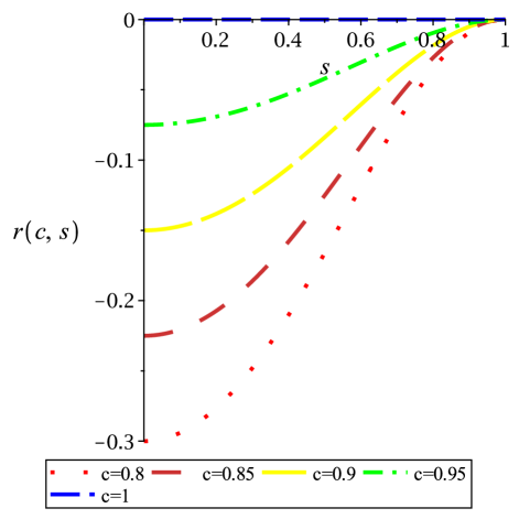
Figure 2: Behaviour of $r(c,s)$, Eq. (29), for different concentrations $c$ of spins with $L=1$. From bottom up: $c=0.8;\,0.85;\,0.9;\,0.95;\,1$ (red, orange, yellow, green and blue curves, coloured online). Value $r(c,s=0)=-\frac{3}{2}(1-c)$ corresponds to the diluted Ising model with non-magnetic impurities.

In the next section we will use available knowledge about RG functions of the model with the effective Hamiltonian (25) together with obtained here dependencies of its bare couplings on spin concentration and length to discuss the effective critical behaviour of the random spin length Ising model.

4 Renormalization group flows and critical exponents

Renormalization group approach is known to be a standard and powerful tool to calculate universal characteristics of critical behaviour, like asymptotic critical exponents and critical amplitude ratios [34, 35]. However, this approach has also been used for a quantitative description of critical behaviour outside an asymptotic regime, where the non-universal effective critical exponents (2) do not yet attain their universal asymptotic values (1). An example is given by a study of flows of couplings under renormalization that describes experimentally observed effective (non-universal) behavior of the amplitude ratio of thermal conductivity in ⁴He, transport coefficients in ³He-⁴He mixture, shear viscosity in Xe (see review [41] for these and other examples). Similar approach has been used to study effective critical behaviour of diluted uniaxial (Ising-like) [31, 32, 33] and Heisenberg [15, 33] magnets. In particular, the field-theoretical RG has been used to explain an experimentally observed impact of concentration of a non-magnetic component on the phase transition into magnetically ordered state. Obtained results show that scenario of an effective critical behaviour depends on the initial couplings of the effective Hamiltonian, that in their turn are dependent on the disorder strength as well.

Before proceeding further, let us rewrite the effective Hamiltonian (28) in a standard notation used in field theoretical RG analysis:

$${\cal H}_{\rm eff}{=}{-}\!\int\!\!d^{d}{\bf R}\!\left\{\!\frac{1}{2}\sum_{\alpha{=}1}^{n}\left[m_{0}^{2}(\phi^{\alpha}_{\bf R})^{2}{+}|\vec{\nabla}\phi^{\alpha}_{\bf R}|^{2}\right]\!{+}\frac{g_{1,0}}{4!}\sum_{\alpha,\beta=1}^{n}(\phi^{\alpha}_{\bf R})^{2}(\phi^{\beta}_{\bf R})^{2}+\frac{g_{2,0}}{4!}\sum_{\alpha=1}^{n}(\phi^{\alpha}_{\bf R})^{4}\!\right\},$$ (31)

where continuous limit has been taken, squared unrenormalized mass $m_{0}^{2}$ measures the temperature distance to the critical point, and the ratio of bare couplings $g_{1,0}/g_{2,0}$ equals to $r(c,s)$, see Eq. 29. A change in couplings $g_{1}$, $g_{2}$ under the renormalization is described by the flow equations [34, 35]:

$$\ell\frac{\rm d}{{\rm d}\ell}g_{1}(\ell)=\beta_{g_{1}}\left(g_{1}(\ell),g_{2}(\ell)\right),\quad\ell\frac{\rm d}{{\rm d}\ell}g_{2}(\ell)=\beta_{g_{2}}\left(g_{1}(\ell),g_{2}(\ell)\right),$$ (32)

where $\ell$ is the flow parameter. The flow parameter can be related by means of a so-called ‘matching condition’ to the correlation length, depending on temperature distance $\tau$ to the critical point, see e.g., Ref. [41]. In simpler case it is proportional to the inverse squared correlation length, therefore the limit $\tau\to 0$ corresponds to $\ell\to 0$. The fixed points ($g_{1}^{*},g_{2}^{*}$) of the system of differential equations (32) are given by:

$$\beta_{g_{1}}\left(g_{1}^{*},g_{2}^{*}\right)=0,\quad\beta_{g_{2}}\left(g_{1}^{*},g_{2}^{*}\right)=0.$$ (33)

A fixed point (FP) is said to be stable if the stability matrix

$$B_{ij}\equiv\partial\beta_{g_{i}}/\partial g_{j},\hskip 30.00005pti,j=1,2,$$ (34)

possesses in this point eigenvalues $\omega_{1},\omega_{2}$ with positive real parts. In the limit $\ell\to 0$, $g_{1}(\ell)$ and $g_{2}(\ell)$ attain the stable FP values $(g_{1}^{*},g_{2}^{*})$. If the stable FP is reachable from the initial conditions (let us recall that for the effective Hamiltonian (31) the initial conditions depend on $c$ and $s$ and lie in the region $g_{2}>0,g_{1}\leq 0$) it corresponds to the critical point of the system. The asymptotic critical exponents are defined by the FP values of the RG $\gamma$-functions. In particular, the isothermal magnetic susceptibility and correlation length exponents $\gamma$ and $\nu$ are expressed in terms of the RG functions $\gamma_{\phi}$ and ${\gamma}_{m^{2}}$ describing renormalization of the field $\phi$ and of the squared mass $m^{2}$ correspondingly [34, 35]:

$$\gamma=\frac{2-2{\gamma}^{*}_{\phi}}{2+{\gamma}^{*}_{m^{2}}},\qquad\nu=\frac{1}{2+{\gamma}^{*}_{m^{2}}}.$$ (35)

In Eq. (35), the superscript means that the corresponding $\gamma$-functions are calculated at a stable FP: $\gamma^{*}_{\phi}\equiv\gamma_{\phi}(g_{1}^{*},g_{2}^{*})$, ${\gamma}^{*}_{m^{2}}\equiv{\gamma}_{m^{2}}(g^{*}_{1},g^{*}_{2})$. In the RG scheme, the effective critical exponents are calculated in the region, where the couplings $(g_{1}(\ell),g_{2}(\ell))$ have not yet reached their fixed point values and depend on $\ell$. In particular, for the exponents $\gamma_{\rm eff}$ and $\nu_{\rm eff}$ one gets [32]:

$$\gamma_{\rm eff}(\tau)=\frac{2-2{\gamma}_{\phi}[g_{1}\{\ell(\tau)\},g_{2}\{\ell(\tau)\}]}{2+{\gamma}_{m^{2}}[g_{1}\{\ell(\tau)\},g_{2}\{\ell(\tau)\}]}+\dots,\quad\nu_{\rm eff}(\tau)=\frac{1}{2+{\gamma}_{m^{2}}[g_{1}\{\ell(\tau)\},g_{2}\{\ell(\tau)\}]}+\dots\,.$$ (36)

In (36) the part denoted by dots is proportional to the $\beta$-functions and comes from the change of the amplitude parts of susceptibility and of correlation length. In the subsequent calculations we will neglect these parts, taking the contribution of the amplitude function to the crossover to be small, as it was used in other studies of disordered systems [31, 32, 15]. However, a more sophisticated approach was developed in Ref. [33] to quantitatively check dependence of effective critical exponents directly on temperature distance to the critical point.

In our study we use the most up-to-date RG functions obtained for the effective Hamiltonian (31) with a record six-loop accuracy in the minimal subtraction renormalization scheme [12] (actually, as a partial case of the RG functions for the cubic model [42]). The series read:

$$\beta_{g_{1}}(g_{1},g_{2}) = -{g_{1}}\left(\varepsilon-\frac{8{g_{1}}}{3}-2{g_{2}}+\frac{14g_{1}^{2}}{3}+\frac{22{g_{1}}{g_{2}}}{3}+\frac{5g_{2}^{2}}{3}+\dots\right),$$ (37)

$$\beta_{g_{2}}(g_{1},g_{2}) = -{g_{2}}\left(\varepsilon-4{g_{1}}-3{g_{2}}+\frac{82g_{1}^{2}}{9}+\frac{46{g_{1}}{g_{2}}}{3}+\frac{17g_{2}^{2}}{3}+\dots\right),$$ (38)

$$\gamma_{\phi}(g_{1},g_{2}) = \frac{g_{1}^{2}}{18}+\frac{{g_{1}}{g_{2}}}{6}+\frac{g_{2}^{2}}{12}+\dots$$ (39)

$$\gamma_{m^{2}}(g_{1},g_{2}) = -g_{2}-\frac{2g_{1}}{3}+\frac{5g_{1}^{2}}{9}+\frac{5{g_{1}}{g_{2}}}{3}+\frac{5g_{2}^{2}}{6}+\dots$$ (40)

Here, $\varepsilon=4-d$ and the dots indicate higher order terms currently known up to $O(g_{i}^{7})$ and $O(g_{i}^{6})$ for the $\beta$- and $\gamma$-functions correspondingly [12, 42].

Starting form the RG expressions one can either develop the $\varepsilon$-expansion, or work directly at $d=3$ considering the renormalized couplings $(g_{1},g_{2})$ as the expansion parameters [43, 44]. However, such RG perturbation theory series are known to be asymptotic at best [35]. One should apply appropriate resummation technique to improve their convergence to get reliable numerical data on their basis. Many different resummation procedures are currently used to this end, see e.g., [4, 5]. In our study we use the method, based on the Borel transformation combined with a conformal mapping [45]. This resummation technique was first elaborated for field-theoretical models with one coupling. It requires knowledge about a high-order behaviour of the series. In particular, for the series

$$f(g)=\sum_{l=0}^{\infty}a_{l}g^{l}$$ (41)

with the known large-order behaviour of the coefficients

$$a_{l}=(-a)^{l}l^{b}l!~{}\left[1+O(1/l)\right],\quad l\to\infty,$$ (42)

where numbers $a$ and $b$ characterize the main divergent part, one can build its resummed counterpart as:

$$f_{\mathrm{R}}(g)=\sum_{l=0}^{\infty}d_{l}(a,b)\int_{0}^{\infty}dt\,\,{{\rm e}^{-t}\,t^{b}\ \left[w(gt)\right]^{l}}\ .$$ (43)

In Eq. (43) $d_{l}(a,b)$ are the coefficients of the re-expansion of the Borel-Leroy image of $f(g)$:

$$B(g)=\sum_{l=0}^{\infty}\frac{a_{l}}{\Gamma(l+b+1)}\ g^{l}\,$$ (44)

which can be written in powers of the new variable $w(g)={\sqrt{1+a\,g}-1\over\sqrt{1+a\,g}+1}$:

$$B(\omega)=\sum_{l=0}^{\infty}d_{l}(a,b)\omega^{l}\,.$$ (45)

$\Gamma(x)$ in (44) is Euler gamma function. This transformation is a conformal mapping of the complex $g$-plane cut from $g=-1/a$ to $-\infty$ onto the unit circle in the $w$-plane such that the singularities of $B(g)$ lying on the negative axis now lie on the boundary of the circle $|w|=1$, see Fig. 3.

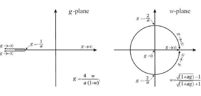
Figure 3: Conformal mapping of the cut-plane onto a disc. See the text for details.

To impose the strong coupling behavior of the series, $f(g\to\infty)\sim g^{\alpha/2}$, Eq. (43) needs to be generalized in the following way [46]

$$f_{\mathrm{R}}(g)=\sum_{l=0}^{\infty}d_{l}(\alpha,a,b)\int_{0}^{\infty}dt\,\,{{\rm e}^{-t}\,t^{b}}\ {\left[w(gt)\right]^{l}\over\left[1-w(gt)\right]^{\alpha}}\,.$$ (46)

This procedure can be extended for field-theoretical models that contain several couplings. For instance, when $f$ is a function of two variables $g_{1}$ and $g_{2}$, the resummation technique can treat $f$ as a function of coupling associated with terms related to the pure (undisordered) magnet (in our case it is $g_{2}$) and a ratio $z=g_{1}/g_{2}$, [47, 22, 48]:

$$f(g_{2},z)=\sum_{l=0}^{\infty}a_{l}(z)\ g_{2}^{l}\,.$$ (47)

Then, keeping $z$ fixed and performing the resummation only in $g_{2}$ according to the steps described above, one gets:

$$f_{\mathrm{R}}(g_{2},z)=\sum_{l=0}^{\infty}d_{l}(\alpha,a(z),b;z)\int_{0}^{\infty}dt\,\,{{\rm e}^{-t}\,t^{b}}{\left[w(g_{2}t;z)\right]^{n}\over\left[1-w(g_{2}t;z)\right]^{\alpha}}\,,$$ (48)

with $z$-dependent parameter $a(z)$. Here, as above, the coefficients $d_{l}(\alpha,a(z),b,z)$ in (48) are computed so that the re-expansion of the right hand side of (48) in powers of $g_{2}$ coincides with that of (47).

Calculation of parameters $a,b,\alpha$ for the field-theoretical models with several couplings is a complicated task. Furthermore, in practice, procedure described above is applied to the truncated series (37)-(40), which are known up to the corresponding order $L$. As a result, the resummed expansions (that usually correspond to certain physical observable) appear to be dependent on resummation parameters $a$, $b$ and $\alpha$. Often applying the conformal Borel method for models with two couplings, such parameters are taken in the region where physical observables are less sensitive to their values, see e.g., Ref. [49]. Although Borel summability is not proven for perturbative series for models with disorder in $d>0$ [47], the conformal Borel method has been successfully used for random Ising model [22, 48, 41, 50] providing accurate critical exponents in agreement with previous analytical estimates. In our analysis we test the region of parameters discussed in the study of five-loop series for the model of frustrated magnet [49]: $a=1/2$, $b$ is varying in the interval $[6,30]$, while $\alpha$ is varying in $[-0.5,2]$. In what follows below we will give more precise values of the parameters.

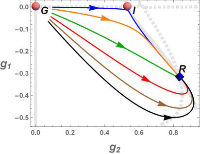
Figure 4: Renormalization group flow in the space of couplings for different initial conditions. From up down: $r=g_{1}(\ell_{0})/g_{2}(\ell_{0})$= -0.01 (blue), -0.1 (orange), -0.3 (green), -0.5 (red), -0.7 (brown), -0.9 (black). Unstable Gaussian (G) and Ising (I) fixed points (shown by red discs) as well as a stable random Ising (R) fixed point (shown by the blue diamond) are located at the intersection points of lines of zeros for functions $\beta_{g_{1}}$ (dashed shadow lines) and $\beta_{g_{2}}$ (solid shadow lines)

To analyze effective critical behaviour, we apply the above described conformal Borel resummation to the $\beta$-functions (37), (38) in the six-loop approximation. In the region of couplings we are interested in one finds three FPs as solutions of Eqs. (33): Gaussian FP G ($g_{1}^{*}=g_{2}^{*}=0$), pure Ising FP I ($g_{1}^{*}=0,\,g_{2}^{*}\neq 0$), and random Ising FP R ($g_{1}^{*}\neq 0,\,g_{2}^{*}\neq 0$), as shown in Fig. 4. For the cases when random Ising FP exists and is a stable locus, our results are compatible with results of Ref. [12] $(g_{1}^{*}\sim-0.3,g_{2}^{*}\sim 0.8)$. As a final choice of the resummation parameters we get $a=1/2$, $b=10$ and $\alpha=1$. We will see below that at such parameter values the asymptotic critical exponents of the random Ising model are very close to the latest analytical estimates (see the Table 1 and the review in Ref. [12]): $\gamma=1.333$ and $\nu=0.676$. Solving numerically the system of differential equations (32) we get the running values of the couplings $(g_{1}(\ell),g_{2}(\ell))$. They define the flow in the parametric space $g_{1}$, $g_{2}$ and in the limit $\ell\to 0$ attain the stable fixed point value (shown by the blue diamond in Fig. 4).

The properties of the flow depend on the initial conditions $(g_{1}(\ell_{0})$, $g_{2}(\ell_{0}))$ for solving the system of differential equations (32). Typical flows obtained for different ratios $g_{1}(\ell_{0})/g_{2}(\ell_{0})=r$ are shown in Fig. 4 by curves of different color. We choose the starting values in the region with the appropriate signs of couplings $g_{1}<0$, $g_{2}>0$ near the origin (in the vicinity of the Gaussian fixed point G shown by the red disc in the Fig. 4). As one sees from the figure, although all RG flows with the decrease of $\ell$ lead to the stable FP, depending on the initial conditions they manifest very different behaviour. For small values of $r$ the flows may first stay within the basin of attraction of the unstable Ising FP (blue curve), with an icrease of $r$ they directly approach the stable random FP (green curve), and further increase of $r$ leads to the ‘overshooting’ behaviour, when the running values of the couplings approach their stable FP values from above (black, brown curves). Let us further analyse, how the observed behaviour of the RG flows is manifest in the effective critical behaviour, in particular, in the values of effective critical exponents.

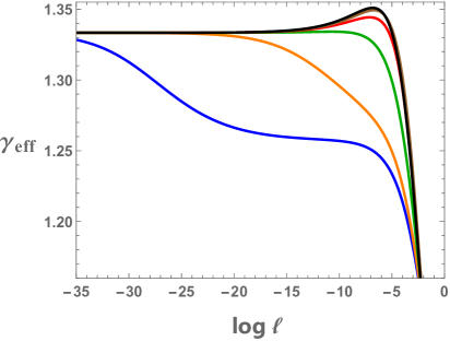
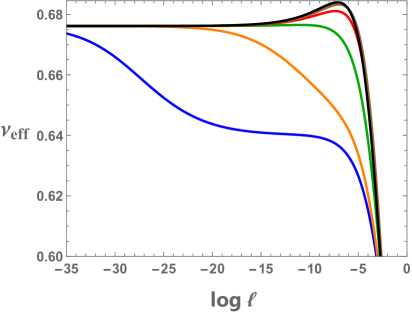
(a)                                                              (b)

Figure 5: Dependencies of the magnetic susceptibility effective critical exponent $\gamma_{\rm eff}$ (a) and the correlation length effective critical exponent $\nu_{\rm eff}$ (b) on the flow parameter calculated along the RG flows of Fig. 2.

Indeed, the running values of couplings presented by flows in Fig. 4 allow to get access to the effective critical exponents. To this end, we apply the above described resummation procedure to the six-loop expansions for the effective critical exponent (36) with the flow-parameter dependent couplings. In this way we get dependencies of the isothermal susceptibility and correlation length effective critical exponents on the flow parameter $\ell$. These are shown in Fig. 5 by corresponding colors. Different regimes in behaviour of couplings $(g_{1},\,g_{2})$ in the course of reaching the stable FP are reflected in different regimes observed for the effective critical exponents when the critical temperature is reached. Depending on the initial conditions, the effective critical exponents either reach their universal values at the stable FP comparatively fast (green curves) or attain the values that differ from the stable FP ones in a broad crossover region. In turn, the crossover region may be either governed by the pure Ising model universality class critical exponents (blue curve) or by the values of the exponents that exceed the stable FP ones (peaks in black and red curves),

For our model (31), the ratio of the initial couplings depends on concentration $c$ and spin length $s$, $r=r(c,s)$ via Eq. (29). Therefore, changing $c$ and $s$ one is able to discriminate between different regimes in the behaviour of the effective critical exponents. To give an example, taking the six-loops stable FP values for $g_{i}^{*}$ from Ref. [12] obtained for different resummations parameters one gets the following estimate for the region of $r$ at the FP: $-0.4<r^{*}<-0.25$. On the other hand, from Eq. (29) one gets the following result for bare (initial) $r$ of the diluted Ising model with concentration of magnetic sites $c=0.8$: $r(c=0.8,s=0)=-0.3$. The closeness of this value to its renormalized counterpart may suggest a direct flow of couplings under renormalization to the stable FP, cf. the green curve in Fig. 4. Such behaviour without almost no correction-to-scaling terms for $c=0.8$ has indeed been observed for this model in MC simulations [51, 52].

5 Conclusions and outlook

In this article, we set ourselves a twofold task. On the one hand, our goal was to show how the disorder in structure alone, without presence of a non-magnetic component can modify the universality class of paramagnetic-ferromagnetic phase transition in uniaxial magnets. On the other hand, we wanted to analyze possible changes in the non-universal effective critical behaviour in such systems. To this end, we considered a random spin length Ising model, when the length $L$ of each spin is a random variable governed by the distribution function $p(L)$ [36, 37].

It is instructive to note, that this model has originally been suggested in the context of sociophysics, where its intention was to describe social interactions and opinion formation between agents of binary nature but of different opinion strength. Here, we used this model to explain phenomenon within the condensed matter physics. We showed that particular cases of this model, a site-diluted Ising model and an Ising model with spins of two different lengths, are described by the effective Hamiltonians (25) and (28) of the same symmetry, hence they belong to the same universality class. This means, that their asymptotic critical exponents (1) are the same. However, effective critical behaviour of these systems differs. We made use of the field-theoretic RG approach to describe such difference quantitatively. Doing so, we reproduce with a high precision the known values of the asymptotic critical exponents in the universality class of the 3d diluted Ising model (compare our results $\gamma=1.333$ and $\nu=0.676$ with that of Ref. [22] given in the fourth line of Table 1).

Furthermore, beyond the narrow region in the vicinity of $T_{c}$, one may observe very different effective critical behaviour even within the same universality class, as we explicitly show in Fig. 5. The effective critical exponents shown there change as $T_{c}$ is approached and, strictly speaking, attain their universal values only at $T_{c}$. Changes in the values of the effective exponents, together with distance to $T_{c}$ depend also on the initial conditions imposed when solving differential equations for the RG flows. The latter, in turn, can be attributed to the microscopic features of the magnet, given in our case by the concentration $c$ and ratio of spin lengths $s$. These features are encoded in the ratio (29) that governs initial conditions for the RG flows. Thus, the scheme implemented here enables one to analyse effective critical behaviour of structurally disordered magnets in a self-consistent way.

The effective critical exponents discussed in this paper can also appear when the critical behaviour is analysed via numerical simulations. Indeed, consider the quotient method [53, 54, 34] as an example. In this method one computes the temperature, $T_{c}(L)$, at which a dimensionless observable, $g(L,T)$ (for instance the Binder cumulant, $B(L,T)$ or the correlation length in units of the lattice size $\xi(L,T)/L$) crosses for lattice sizes $L$ and $2L$: thus, $g(L,T_{c}(L))=g(2L,T_{c}(L))$. Moreover, one can also consider a dimensionful observable which diverges at the critical point as ${\cal O}(L,T_{c})\sim L^{x/\nu}$, where $\nu$ is the correlation length critical exponent. By computing the ratio ${\cal O}(2L,T_{c}(L))/{\cal O}(L,T_{c}(L))$ is possible to write

$$\left.\frac{x}{\nu}\right|_{\infty}=\left.\frac{x}{\nu}\right|_{(L,2L)}+O(\frac{1}{L^{\omega}})\,,$$ (49)

where $\omega$ can be identified with the leading irrelevant eigenvalue in the RG approach [34, 35] and

$$\left.\frac{x}{\nu}\right|_{(L,2L)}\equiv\log_{2}\frac{{\cal O}(2L,T_{c}(L))}{{\cal O}(L,T_{c}(L)}\,,$$ (50)

which can be used as the definition of the effective critical exponent. Notice that in general, in Eq. (49) will not only appear the leading irrelevant eigenvalue of the RG, $\omega$, but all the irrelevant eigenvalues, so the behavior of the effective exponent will not be monotonic in most of the cases. An example of this non-monotonic behavior is the three-dimensional random field Ising model for some observables and different choices of the random magnetic field [55]. Finally, we remark that the finite size scaling theory can be understood using a RG transformation with a RG parameter, $\ell$, given by $\ell=1/L$ [34].

A natural continuation of our study will be the numerical simulation of the random Ising model with two different spin lengths, section 3.2 and analysis of its asymptotic and effective critical behaviour. And – last but not least – search for experimental realizations of the phenomena discussed in this paper.

References

- [1] See e.g., Order, Disorder and Criticality. Advanced Problems of Phase Transition Theory. Yu. Holovatch (editor). vols. 1–7, World Scientific, Singapore, 2004–2022.
- [2] J. Hertz, Disordered Systems, Phys. Scr. T10 (1985) 1. https://doi.org/10.1088/0031-8949/1985/T10/001.
- [3] Vik. S. Dotsenko, Critical phenomena and quenched disorder, Phys. Uspekhi. 38 (1995) 457 [Usp. Fiz. Nauk 165 (1995) 481]. https://doi.org/10.1070/PU1995v038n05ABEH000084.
- [4] R. Folk, Yu. Holovatch, T. Yavors’kii, Critical exponents of a three-dimensional weakly diluted quenched Ising model, Phys. Uspekhi 46 (2003) 169 [Uspekhi Fizicheskikh Nauk 173 (2003) 175]; preprint cond-mat/0106468. https://doi.org/10.1070/PU2003v046n02ABEH001077
- [5] A. Pelissetto, E. Vicari, Critical phenomena and renormalization-group theory, Phys. Rep. 368 (2002) 549. https://doi.org/10.1016/S0370-1573(02)00219-3.
- [6] Yu. Holovatch, V. Blavats’ka, M. Dudka, C. von Ferber, R. Folk, and T. Yavors’kii, Weak quenched disorder and criticality: resummation of asymptotic(?) series, Int. J. Mod. Phys. B 16 (2002) 4027. https://doi.org/10.1142/S0217979202014760.
- [7] Some random magnets were considered as good candidates for magnetic refrigerants, see e. g. Q. Duo, D.Q. Ahoy, M.X.Pan, W. H. Wang, Appl. Phys. Lett. 92 (2008) 011923; Q. Luo, W. H. Wang, J. Non-Crystalline Solids, 355 (2009) 759; Q. Luo, B. Schwartz, N. Mattern, J.J. Eckert, Magnetic ordering and slow dynamics in a Ho-based bulk metallic glass with moderate random magnetic anisotropy, Appl. Phys., 109 (2011) 113904. https://aip.scitation.org/doi/10.1063/1.3594696; V. Singh, P. Bag, R. Rawat, Critical behavior and magnetocaloric effect across the magnetic transition in Sci. Rep. 10 (2020) 6981. https://doi.org/10.1038/s41598-020-63223-0; V. Franco, J.S.Blázquez, J.J.Ipus, J.Y.LawL, M.Moreno-Ramírez, A.Conde, Magnetocaloric effect: From materials research to refrigeration devices, Prog. Mater. Sci. 93 (2-18) (2017) 112. https://doi.org/10.1016/j.pmatsci.2017.10.005; R. Bouachraoui, The magnetocaloric and magnetic properties of the MnFe4Si3: Monte Carlo investigation, Journal of Alloys and Compounds 809 (2019) 151785. https://doi.org/10.1016/j.jallcom.2019.151785.
- [8] G. Grinstein, A. Luther, Application of the renormalization group to phase transitions in disordered systems, Phys. Rev. B 13 (1976) 1329. https://doi.org/10.1103/PhysRevB.13.1329
- [9] R. J. Birgeneau, R. A. Cowley, G. Shirane, H. Joshizawa, D. P. Belanger, A. R. King, and V. Jaccarino, Critical behavior of a site-diluted three-dimensional Ising magnet, Phys. Rev. B 27 (1983) 6747. https://doi.org/10.1103/PhysRevB.27.6747.
- [10] D. P. Belanger, A. R. King, and V. Jaccarino, Crossover from random-exchange to random-field critical behavior in FexZnF2, Phys. Rev. B 34 (1986) 452. https://doi.org/10.1103/PhysRevB.34.452.
- [11] P. W. Mitchell, R. A. Cowley, H. Yoshizawa, P. Böni, Y. J. Uemura, and R. J. Birgeneau, Critical behavior of the three-dimensional site-random Ising magnet: MnxZnF2, Phys. Rev. B 34 (1986) 4719. https://doi.org/10.1103/PhysRevB.34.4719.
- [12] M. V. Kompaniets, A. Kudlis, A. I. Sokolov, Critical behavior of the weakly disordered Ising model: Six-loop expansion study, Phys. Rev. E 103 (2021) 022134. https://doi.org/10.1103/PhysRevE.103.022134.
- [13] T. Egami, Magnetic amorphous alloys: physics and technological applications, Rep. Prog. Phys. 47 (1984) 1601. https://doi.org/10.1088/0034-4885/47/12/002.
- [14] S. N. Kaul, Static critical phenomena in ferromagnets with quenched disorder, J. Magn. Magn. Mater. 53 (1985) 5. https://doi.org/10.1016/0304-8853(85)90128-3.
- [15] M. Dudka, R. Folk, Yu. Holovatch, D. Ivaneiko, Effective critical behaviour of diluted Heisenberg-like magnets, Journ. Magn. Magn. Mater. 256 (2003) 243. https://doi.org/10.1016/S0304-8853(02)00569-3.
- [16] Dinh Chi Linh, Tran Dang Thanh, Le Hai Anh, Van Duong Dao, Hong-Guang Piao, Seong-Cho Yu, Critical properties around the ferromagnetic-paramagnetic phase transition in La0.7Ca0.3-xAxMnO3 compounds (A = Sr, Ba and x = 0, 0.15, 0.3), Journal of Alloys and Compound 725 (2017) 484-495. https://doi.org/10.1016/j.jallcom.2017.07.168.
- [17] E. Bouzaiene, J. Dhahri, E.K. Hlil, H. Belmabrouk, H. Alrobei, Three-dimensional Heisenberg critical phenomena in manganites (x=0 and 0.05), J Mater Sci: Mater Electron, 31 (2020) 18186-18197. https://doi.org/10.1007/s10854-020-04367-7.
- [18] A. Tozri, R. Kamel, W.S. Mohamed, J. Laif, E. Dhahri, and E. K. Hlil, Critical exponents and magnetic entropy change across the continuous magnetic transition in (La, Pr)‑Ba manganites, Applied Physics A 128 (2022) 575. https://doi.org/10.1007/s00339-022-05719-2.
- [19] H. Jaballah, R. Guetari, N. Mliki, L. Bessais, Magnetic properties, critical behavior and magnetocaloric effect in the nanocrystalline , Journ. Phys. Chem. Solids 169 (2022) 110752. https://doi.org/10.1016/j.jpcs.2022.110752.
- [20] A.B. Harris, Upper bounds for the transition temperatures of generalized Ising models, J. Phys. C 7 (1974) 1671. https://doi.org/10.1088/0022-3719/7/17/018.
- [21] R Guida and J. Zinn-Justin, Critical Exponents of the N-vector model, J. Phys. A: Math. Gen. 31 (1998) 8103–8121. https://doi.org/10.1088/0305-4470/31/40/006.
- [22] A. Pelissetto and E. Vicari, Randomly dilute spin models: a six-loop field-theoretic study, Phys. Rev. B 62 (2000) 6393. https://doi.org/10.1103/PhysRevB.62.6393.
- [23] J. S. Kouvel, M.E. Fisher, Detailed Magnetic Behavior of Nickel Near its Curie Point, Phys. Rev. 136 (1964) A1626. https://doi.org/10.1103/PhysRev.136.A1626.
- [24] E. K. Riedel, F. J. Wegner, Effective critical and tricritical exponents, Phys. Rev. B 9 (1974) 294. https://doi.org/10.1103/PhysRevB.9.294.
- [25] E. Zarai, F. Issaoui, A. Tozri, M. Husseinc, E. J. Dhahri, Critical behavior near the paramagnetic to ferromagnetic phase transition temperature in Sr1.5Nd0.5MnO4 compound, Supercond. Nov. Magn., 29 (2016) 869. https://doi.org/10.1007/s10948-015-3367-0.
- [26] J. Makni-Chakrouna, I. Sfifir, W. Cheikhrouhou-Koubaa, M. Koubaa, A. Cheikhrouhou, Structural, magnetic, magnetocaloric effect and critical behavior of La0.7Sr0.3-xMnO3 (), Journ. Magn. Magn. Mater. 432 (2017) 484. https://doi.org/10.1016/j.jmmm.2017.01.100.
- [27] K.-Y. Hou, Q.-Y. Dong, L. Su, X.-Q. Zhang, Z.-H. Cheng, Three-dimensional Heisenberg critical behavior in amorphous Gd65Fe20Al15 and Gd71Fe3Al26 alloys, Journal of Alloys and Compounds 788 (2019) 155. https://doi.org/10.1016/j.jallcom.2019.02.212.
- [28] M. Chebaane, Ma. Oumezzine, R. Bellouz, E. K. Hlil, A. Fouzri, Study of Critical Magnetic Behaviour in Nanocrystalline La0.65Ce0.05Sr0.3Mn1-xCuxO3 (x=0, x=0.05 and x=0.15) Prepared by Pechini Method, Journal of Superconductivity and Novel Magnetism 34 (2021) 193. https://doi.org/10.1007/s10948-020-05568-1.
- [29] P. Gebara, M. Hasiak, Determination of Phase Transition and Critical Behavior of the As-Cast GdGeSi-(X) Type Alloys (Where X = Ni, Nd and Pr), Materials 14 (2021) 185. https://doi.org/10.3390/ma14010185.
- [30] A. Perumal, V. Srinivas, V. V. Rao, R. A. Dunlap, Quenched Disorder and the Critical Behavior of a Partially Frustrated System, Phys. Rev. Lett. 91 (2003) 137202. https://doi.org/10.1103/PhysRevLett.91.137202.
- [31] H.K. Janssen, K. Oerding, and E. Sengespeick, On the crossover to universal criticality in dilute Ising systems, J. Phys. A 28 (1995) 6073. https://doi.org/10.1088/0305-4470/28/21/012.
- [32] R. Folk, Yu. Holovatch, and T. Yavors’kii, Effective and asymptotic critical exponents of a weakly diluted quenched Ising model: Three-dimensional approach versus expansion, Phys. Rev. B 61 (2000) 15114. https://doi.org/10.1103/PhysRevB.61.15114.
- [33] P. Calabrese, P. Parruccini, A. Pelissetto, E. Vicari, Crossover behavior in three-dimensional dilute spin systems, Phys. Rev. E 69 (2004) 036120. https://doi.org/10.1103/PhysRevE.69.036120.
- [34] D. J. Amit and V. Martín Mayor, Field Theory, The Renormalization Group and Critical Phenomena, (World Scientific Publishing, 2005). https://doi.org/.
- [35] See e.g., J. Zinn-Justin, Quantum Field Theory and Critical Phenomena (International Series of Monographs on Physics, 92), Oxford Univ Press, 1996; H. Kleinert, V. Schulte-Frohlinde, Critical Properties of -Theories, World Scientific, Singapore, 2001.
- [36] M. Krasnytska, B. Berche, Yu. Holovatch, R. Kenna, Generalized Ising Model on a Scale-Free Network: An Interplay of Power Laws, Entropy 23(9) (2021) 1175. https://doi.org/10.3390/e23091175.
- [37] M. Krasnytska, B. Berche, Yu. Holovatch, R. Kenna, Ising model with variable spin/agent strengths, J. Phys.: Complexity 1 (2020) 035008. https://doi.org/10.1088/2632-072X/abb654.
- [38] R. Brout, Statistical Mechanical Theory of a Random Ferromagnetic System, Phys. Rev. 115 (1959) 824. https://doi.org/10.1103/PhysRev.115.824.
- [39] V. Dotsenko, Introduction to the Replica Theory of Disordered Statistical Systems. Cambridge: Cambridge University Press, 2001. https://doi.org/10.1017/CBO9780511524592.
- [40] J. M. Yeomans, R. B. Stinchcombe, Critical properties of site- and bond-diluted Ising ferromagnets, J. Phys. C: Solid State Phys. 12 (1979) 347. https://doi.org/10.1088/0022-3719/12/2/022.
- [41] R. Folk, G. Moser, Critical dynamics: a field-theoretical approach, J. Phys. A: Math. Gen. 39 (2006) R207. https://doi.org/10.1088/0305-4470/39/24/R01.
- [42] L. T. Adzhemyan, E. V. Ivanova, M. V. Kompaniets, A. Kudlis, and A. I. Sokolov, Six-loop expansion study of three-dimensional n-vector model with cubic anisotropy Nucl. Phys. B 940 (2019) 332. https://doi.org/10.1016/j.nuclphysb.2019.02.001.
- [43] R. Schloms, V. Dohm, Renormalization-Group Functions and Nonuniversal Critical Behaviour, Europhys. Lett. 3 (1987) 413. https://doi.org/10.1209/0295-5075/3/4/005.
- [44] R. Schloms, V. Dohm, Minimal renormalization without -expansion: Critical behavior in three dimensions, Nucl. Phys. B 328 (1989) 639. https://doi.org/10.1016/0550-3213(89)90223-X.
- [45] J. C. Le Guillou and J. Zinn-Justin, Critical Exponents for the n-Vector Model in Three Dimensions from Field Theory, Phys. Rev. Lett. 39 (1977) 95. https://doi.org/10.1103/PhysRevLett.39.95.
- [46] D.I. Kazakov, O.V. Tarasov, D.V. Shirkov, Analytic continuation of the results of perturbation theory for the model g to the region , Theor. Math. Phys. 38 (1979) 9-16. https://doi.org/10.1007/BF01030252.
- [47] G. Alvarez, V. Martin-Mayor, J. J. Ruiz-Lorenzo, Summability of the perturbative expansion for a zero-dimensional disordered spin model, J. Phys. A 33 (2000) 841. https://doi.org/10.1088/0305-4470/33/5/302.
- [48] P. Calabrese, P. Parruccini, A. Pelissetto, E. Vicari, Critical behavior of O(2) O(N) symmetric models, Phys. Rev. B 70 (2004) 174439. https://doi.org/10.1103/PhysRevB.70.174439.
- [49] B Delamotte, Yu. Holovatch, D. Ivaneyko, D. Mouhanna, M. Tissier, Fixed points in frustrated magnets revisited, J. Stat. Mech. (2008) P03014. https://doi.org/10.1088/1742-5468/2008/03/P03014.
- [50] A.S. Krinitsyn, V.V. Prudnikov, P.V. Prudnikov, Calculations of the dynamical critical exponent using the asymptotic series summation method, Theor. Math. Phys. 147 (2006) 561. https://doi.org/10.1007/s11232-006-0063-z.
- [51] H.G. Ballesteros, L.A. Fernández, V. Martín-Mayor, A. Muñoz Sudupe, G. Parisi, and J. J. Ruiz-Lorenzo, Critical exponents of the three-dimensional diluted Ising model, Phys. Rev. B 58 (1998) 2740. https://link.aps.org/doi/10.1103/PhysRevB.58.2740.
- [52] P. Calabrese, V. Martín-Mayor, A. Pelissetto, E. Vicari, The three-dimensional randomly dilute Ising model: Monte Carlo results, Phys. Rev. E 68 (2003) 036136 https://doi.org/10.1103/PhysRevE.68.036136.
- [53] F. Cooper, B. Freedman and D. Preston, Solving 4 field theory with Monte Carlo, Nucl. Phys. B 210 (1982) 210. https://doi.org/10.1016/0550-3213(82)90240-1.
- [54] H.G. Ballesteros, L.A. Fernandez, V. Martin-Mayor, A. Munoz-Sudupe, G. Parisi and J. J. Ruiz-Lorenzo, The four-dimensional site-diluted Ising model: A finite-size scaling study, Nuclear Physics B 512 (1998) 681. https://doi.org/10.1016/S0550-3213(97)00797-9.
- [55] N. Fytas and V. Martin-Mayor, Universality in the Three-Dimensional Random-Field Ising Model, Phys. Rev. Lett. 110, 227201 (2013). https://doi.org/10.1103/PhysRevLett.110.227201.