Trace Expressions and Associated Limits for Non-Equilibrium Casimir Torque

Abstract

We exploit fluctuational electrodynamics to present trace expressions for the torque experienced by arbitrary objects in a passive, non-absorbing, rotationally invariant background environment. Specializing to a single object, this formalism, together with recently developed techniques for calculating bounds via Lagrange duality, is then used to derive limits on the maximum Casimir torque that a single object with an isotropic electric susceptibility can experience when out of equilibrium with its surrounding environment. The maximum torque achievable at any wavelength is shown to scale in proportion to body volumes in both subwavelength (quasistatics) and macroscopic (ray optics) settings, and come within an order of magnitude of achievable torques on topology optimized bodies. Finally, we discuss how to extend the formalism to multiple bodies, deriving expressions for the torque experienced by two subwavelength particles in proximity to one another.

Over the past decades, much effort has been devoted to understanding fluctuation phenomena in structured media Biehs et al. [2021], Woods et al. [2016]. For example, in recent years Casimir forces have been considered in a variety of systems out of thermal equilibrium, including planar slabs Antezza et al. [2008], spheres Krüger et al. [2011, 2011, 2012], Müller and Krüger [2016], cylinders Golyk et al. [2012], and gratings Noto et al. [2014]. Whether through surface texturing or by enforcing far out of equilibrium conditions, the Casimir force can be made to exhibit a wide range of power laws Antezza et al. [2006], lead to unstable and stable equilibria Krüger et al. [2011], become repulsive Antezza et al. [2008], Krüger et al. [2011, 2011], and lead to self-propulsion Krüger et al. [2011], Müller and Krüger [2016]. In anisotropic media or systems exhibiting chirality, thermal fluctuations can also cause objects to exchange net angular momentum with their environments or other nearby objects, resulting in a net torque Kats [1971], Khandekar et al. [2021], Parsegian and Weiss [1972], Guo and Fan [2021], Gao et al. [2021], a prediction that was recently verified in experiments Somers et al. [2018]. As interest in mechanical devices of increasingly smaller scales continues to grow, so too is the ability to exploit fluctuation phenomena such as laser shot noise and the Casimir effect to actuate nanocale rotors Ding et al. [2022], van der Laan et al. [2021], Stickler et al. [2021].

In this paper, we exploit the mathematical framework of fluctuational electrodynamics Rytov et al. [1989], Otey et al. [2014] and scattering theory Rahi et al. [2009] to rigorously derive trace expressions for the thermal Casimir torque experienced by a set of objects out of equilibrium with themselves or their environment. Based on the dyadic Green’s function $\mathbb{G}_{0}$ of a rotationally invariant background environment and the scattering $\mathbb{T}$ operators of each object in isolation, these expressions, valid also for arbitrary anisotropic bodies, are extensions of analogous and recently derived power and force quantities Krüger et al. [2012]. Special attention is given to the case of a single body embedded in a background environment as well as two-body scenarios, generalizing recent expressions for the torque on dipolar particles Manjavacas and De Abajo [2010a, b], Guo and Fan [2021], Khandekar et al. [2021]. Furthermore, employing Lagrange duality in the case where the single body is composed of an isotropic electric susceptibility, we present upper bounds on the frequency contributions to the non-equilibrium Casimir torque possible for arbitrarily structured objects confined within a bounding sphere. These bounds show that the maximum torque experienced by a body scales like the volume of the object in both the small particle (quasistatics) and large-body (ray optics) limits, a feature unique to torque as both heat transfer and forces are known to scale like area in the large-size limit Molesky et al. [2019a], Woods et al. [2016]. Finally, our expressions are valid for arbitrary geometries and take simple forms in the limit of dipolar particles, which we illustrate by deriving expressions involving torque between two subwavelength bodies out of equilibrium and in the vicinity of one another. For clarity and conciseness, the main text focuses on fundamental equations and results, leaving detailed derivations and technical discussions to the appendix; interested readers are encouraged to consult the appendix for additional insights.

I General Force and Torque Formulas

The net force and torque on a body resulting from a set of prescribed electromagnetic fields $\bm{\mathrm{E}}$ and $\bm{\mathrm{B}}$ acting on it can be derived from the Lorentz force law , and are given by (using Einstein convention):

$$\mathbf{F} =\int_{V}d^{3}\mathbf{r}\int_{-\infty}^{\infty}d\omega\left[\rho^{*}(\omega,\mathbf{r})\mathbf{E}(\omega,\mathbf{r})+\mathbf{J}^{*}(\omega,\mathbf{r})\times\mathbf{B}(\omega,\mathbf{r})\right]$$ (1)

$$=\int_{V,\omega}\left[\frac{i}{\omega}(\nabla\cdot\mathbf{J}^{*})\mathbf{E}-\frac{i}{\omega}\mathbf{J}^{*}\times(\nabla\times\mathbf{E})\right],$$ (2)

$$=\int_{V,\omega}\frac{i}{\omega}\left[(\nabla\cdot\mathbf{J}^{*})\mathbf{E}-\mathbf{J}^{*}\cdot\nabla\mathbf{E}(\omega,\mathbf{r})+(\mathbf{J}^{*}\cdot\nabla)\mathbf{E}\right],$$ (3)

$$=\int_{V,\omega}\frac{i}{\omega}\left[\frac{\partial J_{j}^{*}}{\partial r_{j}}E_{k}\mathbf{e}_{k}-J_{j}^{*}\frac{\partial E_{j}}{\partial r_{k}}\mathbf{e}_{k}+J_{j}^{*}\frac{\partial E_{k}}{\partial r_{j}}\mathbf{e}_{k}\right],$$ (4)

$$=\int_{V}d^{3}\mathbf{r}\int_{-\infty}^{\infty}d\omega\frac{1}{\hbar\omega}\left[J_{a}^{*}\hat{\mathbf{p}}E_{a}+i\hbar\frac{\partial}{\partial r_{j}}(J_{j}^{*}E_{k})\mathbf{e}_{k}\right]$$ (5)

$$\bm{\tau} =\int_{V}d^{3}\mathbf{r}\int_{-\infty}^{\infty}d\omega\mathbf{r}\times\left[\rho^{*}(\omega,\mathbf{r})\mathbf{E}(\omega,\mathbf{r})+\mathbf{J}^{*}(\omega,\mathbf{r})\times\mathbf{B}(\omega,\mathbf{r})\right]$$ (6)

$$=\int_{V,\omega}\frac{i}{\omega}\mathbf{r}\times\left[(\nabla\cdot\mathbf{J}^{*})\mathbf{E}-\mathbf{J}^{*}\times(\nabla\times\mathbf{E})\right]$$ (7)

$$=\int_{V,\omega}\frac{i}{\omega}\mathbf{e}_{m}\epsilon_{mjk}[-r_{j}J_{a}^{*}(\partial_{k}E_{a})+\partial_{a}(r_{j}J_{a}^{*}E_{k})-J_{j}^{*}E_{k}]$$ (8)

$$=\int_{V}d^{3}\mathbf{r}\int_{-\infty}^{\infty}d\omega\frac{1}{\hbar\omega}[J_{a}^{*}\hat{\mathbf{L}}E_{a}+\mathbf{J}^{*}\hat{\mathbf{S}}\mathbf{E}+$$

$$\qquad\qquad\qquad\qquad\ \ \ \ i\hbar\mathbf{e}_{m}\epsilon_{mjk}\partial_{a}(r_{j}J_{a}^{*}E_{k})]$$ (9)

where $\hat{\mathbf{L}}=\mathbf{r}\times\hat{\mathbf{p}}=-i\hbar\mathbf{r}\times\nabla$ and

$$\hat{\mathbf{S}}=-i\hbar\Bigg{\{}\begin{bmatrix}0&0&0\\ 0&0&1\\ 0&-1&0\end{bmatrix},\begin{bmatrix}0&0&-1\\ 0&0&0\\ 1&0&0\end{bmatrix},\begin{bmatrix}0&1&0\\ -1&0&0\\ 0&0&0\end{bmatrix}\Bigg{\}},$$ (10)

are the orbital and spin angular momentum operators, respectively Khersonskii et al. , defined in the Cartesian basis and compactly summarized by $(\hat{S}_{a})_{bc}=-i\hbar\epsilon_{abc}$. In deriving the expressions above, we made use of the continuity equation $i\omega\rho(\omega,\mathbf{r})=\nabla\cdot\mathbf{J}(\omega,\mathbf{r})$, Faraday’s law $\mathbf{B}(\omega,\mathbf{r})=\frac{1}{i\omega}\nabla\times\mathbf{E}(\omega,\mathbf{r})$, and the following algebraic identities:

$$\mathbf{r}\times(\mathbf{J}^{*}(\omega,\mathbf{r})\times(\nabla\times\mathbf{E}(\omega,\mathbf{r})))$$

$$=\mathbf{e}_{i}\epsilon_{ijk}r_{j}(\mathbf{J}^{*}(\omega,\mathbf{r})\times(\nabla\times\mathbf{E}(\omega,\mathbf{r})))_{k}$$

$$=\mathbf{e}_{i}\epsilon_{ijk}r_{j}(J_{a}^{*}(\partial_{k}E_{a})-J_{a}^{*}(\partial_{a}E_{k}))$$

$$=\mathbf{e}_{i}\epsilon_{ijk}(r_{j}J_{a}^{*}(\partial_{k}E_{a})-\partial_{a}(r_{j}J_{a}^{*}E_{k})$$

$$\hskip 86.72377pt+\delta_{aj}J_{a}^{*}E_{k}+r_{j}(\partial_{a}J_{a}^{*})E_{k})$$

and $\mathbf{r}\times(\nabla\cdot\mathbf{J}^{*}(\omega,\mathbf{r}))\mathbf{E}(\omega,\mathbf{r})=\mathbf{e}_{i}\epsilon_{ijk}r_{j}E_{k}(\partial_{a}J_{a}^{*})$.

Notably, the total derivative terms $\sim\partial_{a}(r_{j}J_{a}^{*}E_{k})$ above vanish in scenarios in which there are no net currents just outside the body. In fact, Eq. (5) minus the total derivative terms has been used as the starting point for deriving trace expressions for the Casimir force Krüger et al. [2012], Müller and Krüger [2016], Krüger et al. [2011], Gelbwaser-Klimovsky et al. [2021]. In considering torque, one might naively though incorrectly insert $\mathbf{r}\times$ into prior trace expressions for forces Krüger et al. [2012], Müller and Krüger [2016], Krüger et al. [2011], introducing terms of the form $\mathbf{r}\times\nabla$ and thus leading to quantities proportional to the orbital angular momentum operator $\hat{\mathbf{L}}=\mathbf{r}\times\hat{\mathbf{p}}=-i\hbar\mathbf{r}\times\nabla.$ Specifically, while the $J_{a}^{*}\hat{\mathbf{L}}E_{a}$ term above would follow upon inserting $\mathbf{r}\times$ into the force expression of Eq. (5), such naive manipulation would miss the additional term $\mathbf{J}^{*}\hat{\mathbf{S}}\mathbf{E}=-i\hbar\mathbf{J}^{*}\times\mathbf{E}$ present in Eq. (9). The presence of this last term should be expected on physical grounds: a photon is a spin-1 particle, and the torque exerted by a vector field does not just depend on angular derivatives (“orbital” contributions), but also on the mixing of different vector components (“spin” contributions).

II Casimir Torque on a Single Body

Starting from the above general expression, one can derive a corresponding expression for the Casimir torque on a collection of objects, the origin of which are thermal fluctuations of currents and fields in matter and throughout space. The relation quantifying the statistical thermodynamics of matter and resulting charge fluctuations is known as the fluctuation-dissipation theorem (FDT), and takes the form Novotny and Hecht [2012], Bimonte et al. [2017a]

$$\langle J_{i}(\mathbf{x},\omega)J_{j}^{*}(\mathbf{x}^{\prime},\omega^{\prime})\rangle_{T}\\ =\frac{\omega\epsilon_{0}}{2\pi}\coth\left(\frac{\hbar\omega}{2k_{B}T}\right)\bm{\chi}_{ij}^{\mathsf{A}}(\mathbf{x},\mathbf{x}^{\prime};\omega)\delta(\omega-\omega^{\prime}),$$ (11)

with $\langle\cdots\rangle_{T}$ denoting an equilibrium thermal average of the electric current sources in a medium of general electric susceptibility $\bm{\chi}$ held at a temperature $T$. The superscript $\mathsf{A}$ on an operator $\Theta$ denotes its asymmetric part, $\Theta^{\mathsf{A}}\equiv\frac{1}{2i}(\Theta-\Theta^{\dagger}),$ where $\dagger$ denotes conjugate transpose. In our notation, $\Theta_{ab}^{\dagger}(\mathbf{x},\mathbf{y})=\Theta_{ba}(\mathbf{y},\mathbf{x})^{*}$, treating the vector component and spatial coordinate as an index pair. For systems in thermal equilibrium, the current–current correlations along with Maxwell’s equations can be used to derive corresponding field–field correlations, $\mathbb{C}_{ij}^{eq}(T,\omega,\omega^{\prime};\mathbf{r},\mathbf{r}^{\prime})\equiv\langle E_{i}(\mathbf{r},\omega)E_{j}^{*}(\mathbf{r}^{\prime},\omega^{\prime})\rangle_{T}=\frac{\hbar\omega^{2}}{2\pi c^{2}\epsilon_{0}}\coth\left(\frac{\hbar\omega}{2k_{B}T}\right)\delta(\omega-\omega^{\prime})\mathbb{G}^{\mathsf{A}}_{ij}(\omega;\mathbf{r},\mathbf{r}^{\prime})$, in terms of the Green’s function of the system $\mathbb{G}$, defined by $\left[\nabla\times\nabla\times-\mathbb{V}-\frac{\omega^{2}}{c^{2}}\mathbb{I}\right]\mathbb{G}(\mathbf{r},\mathbf{r}^{\prime})=\mathbb{I}\delta^{(3)}(\mathbf{r}-\mathbf{r}^{\prime})$ where $\mathbb{V}=\frac{\omega^{2}}{c^{2}}(\mathbb{\epsilon}-\mathbb{I})+\nabla\times(\mathbb{I}-\mathbb{\mu}^{-1})\nabla\times$ is the potential or generalized susceptibility introduced by the objects Bimonte et al. [2017a]. In a nonequilibrium stationary state, each object is assumed to be at local equilibrium, such that the current fluctuations within each object satisfy the FDT at the appropriate local temperature. The details of the use of FDT and local equilibrium properties with the scattering equations have been described before Bimonte et al. [2017a], Krüger et al. [2012] and laid out in the appendix. Detailed derivations and use of similar principles to derive force expressions can be found in Refs. Krüger et al. [2012], Müller and Krüger [2016]. Here, we restrict our attention to torque.

As a concrete example, we consider the Casimir torque on an isolated body out of equilibrium with its surroundings. To begin with, we use the linear response relation between the set of sources in the body and resulting fields, $\mathbf{E}=i\mu_{0}\omega\mathbb{G}_{0}\mathbf{J}$, to rewrite the thermally averaged torque in terms of the field–field correlation Dyadic:

$$\bm{\tau} =\textrm{Re}\int_{V_{body}}d^{3}\mathbf{r}\int_{-\infty}^{\infty}d\omega\frac{1}{\hbar\omega}[J_{a}^{*}\hat{\mathbf{L}}E_{a}+\mathbf{J}^{*}\hat{\mathbf{S}}\mathbf{E}]$$ (12)

$$=-\textrm{Im}\int_{V_{body}}d^{3}\mathbf{r}\int_{-\infty}^{\infty}d\omega\frac{1}{\hbar\omega^{2}\mu_{0}}[(\mathbb{G}_{0}^{-1}\mathbf{E})_{a}^{*}\hat{\mathbf{L}}E_{a}+$$

$$\qquad\qquad\qquad\qquad\qquad\qquad\qquad(\mathbb{G}_{0}^{-1}\mathbf{E})^{*}\hat{\mathbf{S}}\mathbf{E}]$$ (13)

$$=-\textrm{Im}\int_{-\infty}^{\infty}d\omega\frac{1}{\hbar\omega^{2}\mu_{0}}\text{Tr}|_{V_{body}}[\hat{\mathbf{J}}\mathbb{C}\mathbb{G}_{0}^{-1\dagger}],$$ (14)

where $\hat{\mathbf{J}}=\hat{\mathbf{L}}+\hat{\mathbf{S}}$ is the total angular momentum operator and the trace is taken over the vector components and position arguments. The final line follows by taking an ensemble average $\langle\bm{\tau}\rangle$ of the torque, expanding the integrand, and replacing $\langle E_{a}(\mathbf{r},\omega)E_{b}^{*}(\mathbf{r}^{\prime},\omega)\rangle$ by the field-field correlator $\mathbb{C}_{ab}(\mathbf{r},\mathbf{r}^{\prime}).$ The notation $|_{V_{body}}$ denotes that the outer-most indices of the operator are traced over positions in the body, while all others are over all space. The operator $\mathbb{G}_{0}$ represents the background Green’s function, which in vacuum satisfies $\left[\nabla\times\nabla\times-\frac{\omega^{2}}{c^{2}}\mathbb{I}\right]\mathbb{G}_{0}(\mathbf{r},\mathbf{r}^{\prime})=\mathbb{I}\delta^{(3)}(\mathbf{r}-\mathbf{r}^{\prime}).$ All of the statistical properties of the sources in Eq. (14) are represented by the field–field correlation Dyadic $\mathbb{C}$ which, in the out of equilibrium setting, can be decomposed $\mathbb{C}^{neq}(T_{env},T_{body})=\mathbb{C}^{eq}(T_{env})+[\mathbb{C}_{body}^{src}(T_{body})-\mathbb{C}_{body}^{src}(T_{env})]$ as a sum of an equilibrium $\mathbb{C}^{eq}(T_{env})$ plus a non-equilibrium term stemming from the difference of the temperatures of the body and environment, with the contribution due to the sources in the body (as opposed to the environment) at a local temperature $T$ given by Krüger et al. [2012],

$$\mathbb{C}_{body}^{src}(T)=\text{sgn}(\omega)\frac{\hbar\omega^{2}}{\pi c^{2}\epsilon_{0}}n(|\omega|,T)\mathbb{G}_{0}\left(\mathbb{T}^{\mathsf{A}}-\mathbb{T}\mathbb{G}_{0}^{\mathsf{A}}\mathbb{T}^{\dagger}\right)\mathbb{G}_{0}^{\dagger},$$

where $n(\omega,T)=\frac{1}{\exp(\frac{\hbar\omega}{k_{B}T})-1}$ is the Bose–Einstein distribution function. The scattering $\mathbb{T}$ operator introduced above transforms incident fields into induced currents in the body Rahi et al. [2009], and is formally defined by the relation $\mathbb{T}=\mathbb{V}(\mathbb{I}-\mathbb{G}_{0}\mathbb{V})^{-1}.$ Plugging the field–field correlator $\mathbb{C}^{neq}(T_{env},T_{body})$ into Eq. (14) yields

$$\bm{\tau} =-\textrm{Im}\int_{0}^{\infty}d\omega\,[n(\omega,T_{body})-n(\omega,T_{env})]$$

$$\qquad\qquad\times\frac{2}{\pi}\text{Tr}[\hat{\mathbf{J}}\mathbb{G}_{0}\big{(}\mathbb{T}^{\mathsf{A}}-\mathbb{T}\mathbb{G}_{0}^{\mathsf{A}}\mathbb{T}^{\dagger}\big{)}]$$ (15)

$$=\int_{0}^{\infty}d\omega[n(\omega,T_{body})-n(\omega,T_{env})]$$

$$\qquad\qquad\times\underbrace{\frac{2}{\pi}\text{Tr}[(-\hat{\mathbf{J}}\mathbb{G}_{0}^{\mathsf{A}})\big{(}\mathbb{T}^{\mathsf{A}}-\mathbb{T}\mathbb{G}_{0}^{\mathsf{A}}\mathbb{T}^{\dagger}\big{)}]}_{\Phi_{J}(\omega)}$$ (16)

The Tr symbol denotes a trace over the complete set of indices of the enclosed operators (for example, both the position and polarization indices of the dipole sources). The switch from $\text{Tr}|_{V_{body}}$ to Tr is possible since $\mathbb{C}_{body}^{src}\mathbb{G}_{0}^{-1\dagger}$ has $\mathbb{T}$ or $\mathbb{T}^{\dagger}$ on the left or right of each term in the expansion. As $\mathbb{T}$ vanishes for all points outside $V_{body}$, one can extend the spatial integration to be over all space, resulting in a trace expression. Furthermore, in going to the final expression above, we used the Hermiticity of the quantity in parenthesis and assumed a background environment with rotational symmetry (so that $\mathbb{G}_{0}$ and $\hat{\mathbf{J}}$ commute) in which case, since $\hat{\mathbf{J}}$ is Hermitian, $(\hat{\mathbf{J}}\mathbb{G}_{0})^{\mathsf{A}}=\hat{\mathbf{J}}\mathbb{G}_{0}^{\mathsf{A}}.$ The assumption that $\mathbb{G}_{0}$ describes a rotationally symmetric background is the only symmetry assumption needed to arrive at the final expression Eq. (16). In particular, note that $\mathbb{V}$ can be anisotropic or nonreciprocal.

The purely algebraic quantity $\Phi_{J}$ depends only on geometric and material properties and can be directly interpreted as angular momentum exchanged between the object and its environment, with $-(\mathbb{T}^{\mathsf{A}}-\mathbb{T}\mathbb{G}_{0}^{\mathsf{A}}\mathbb{T}^{\dagger})\hat{\mathbf{J}}$ describing absorption expressed as the subtraction of scattered angular momentum from net extracted (extinction) angular momentum: namely, the first term quantifies angular momentum extracted from an incident wave upon interaction with the body while the second describes angular momentum carried away by the scattered field. Note that since fluctuations at different frequencies are uncorrelated, as per Eq. (11), the total rate of angular momentum transfer is therefore given by an integral over all frequencies, with each frequency contribution weighted by a difference of thermal occupation numbers.

In general, the calculation of trace expressions for forces in the basis of vector spherical harmonics (VSH) is complicated by the fact that the matrix representation of $\hat{\mathbf{p}}$ is not diagonal in this basis Khersonskii et al. . Introducing multiple bodies adds further complications. However, beyond its logical necessity, the appearance of the total angular momentum $\hat{J}_{z}\equiv\hat{L}_{z}+\hat{S}_{z}$ in torque trace expressions offers computational advantages for torque calculations compared to force calculations. In the basis of VSH, $\hat{J}_{z}$ is diagonal Khersonskii et al. , suggesting that torque calculations in certain physical setups might be simpler analytically and numerically than the corresponding force calculations. As an illustrative example, we first consider bounds on the maximum non-equilibrium torque that a single compact body may experience.

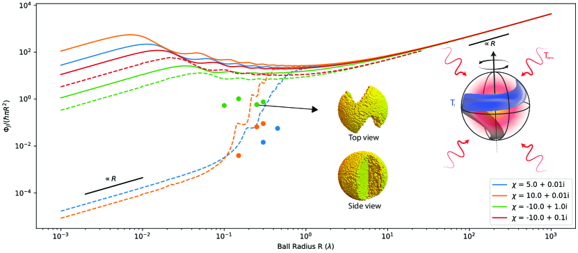
Figure 1: Bounds on maximum angular momentum transfer based on the conservation of energy. An isolated body out of equilibrium can exchange net angular momentum with the environment, illustrated by an inset schematic. The figure shows the maximum spectral angular momentum transfer $\Phi_{J}(\omega)$ (defined in the main text) at a single wavelength $\lambda$ allowed for a body enclosed in a spherical design volume of radius $R$, for multiple values of body material susceptibilities $\chi(\omega)$, captured by the material factor $\lVert\chi(\omega)\rVert^{2}/\imaginary\left[\chi(\omega)\right].$ $\Phi_{J,max}(\omega)$ is seen to smoothly blend the intuitively expected $\propto V$ behaviors of quasi-static and ray-optic regimes, with an intermediate regime of growing radiative losses that suppresses the overall prefactor in the volumetric scaling. The full bounds, involving a relaxation of physics through the conservation of energy or optical theorem Jackson [1999], described in App. F, are shown as dashed lines. Solid lines describe a semi-analytical bound that, while looser owing to additional relaxations, provides an intuitive picture of the various wave contributions to torque (see main text). The dots indicate values of $\Phi_{J}(\omega)$ observed in topology optimized structures Polimeridis et al. [2014, 2015], Polimeridis .

II.1 Size scaling and maximum torque

Equation (16) is valid for arbitrarily structured objects of any size and shape. As the VSHs are eigenstates of $\hat{J}_{z},$ it is convenient to express the underlying scattering operators in a spectral basis of VSHs Khersonskii et al. , Tsang et al. [2004]; choosing the origin to lie at the center of mass, the vacuum Green’s function can be written as $\mathbb{G}_{0}^{\mathsf{A}}=\sum_{P,j,m}\left|P,j,m\right>\left<P,j,m\right|$ (the eigenvalues are not explicitly factored out, allowing for easier extraction of scaling behavior below) and the net angular momentum exchange as $\Phi_{J}(\omega)=-\frac{2\hbar}{\pi}\sum_{\begin{subarray}{c}Pjm\\ P^{\prime}j^{\prime}m^{\prime}\end{subarray}}m(\textrm{Im}[\mathcal{T}_{Pjm;P^{\prime}j^{\prime}m^{\prime}}]\delta_{P^{\prime}j^{\prime}m^{\prime};Pjm}-\mathcal{T}_{Pjm;P^{\prime}j^{\prime}m^{\prime}}\mathcal{T}_{Pjm;P^{\prime}j^{\prime}m^{\prime}}^{*})$ in terms of the matrix elements of the $\mathbb{T}$ operator, $\mathcal{T}_{Pjm;P^{\prime}j^{\prime}m^{\prime}}\equiv\left<P,j,m\left|\mathbb{T}\right|P^{\prime},j^{\prime},m^{\prime}\right>$. It follows that objects for which the scattering operator satisfies $\mathcal{T}_{P,j,m;P^{\prime},j^{\prime},m^{\prime}}=\mathcal{T}_{P,j,-m;P^{\prime},j^{\prime},-m^{\prime}}$ (for example, spherically or cylindrically symmetrical bodies), exhibit zero Casimir torque, owing to the lack of a preferred direction of radiation. Intuitively, for small objects (particles), the scaling of the lowest order scattering elements $\mathcal{T}_{N1m,N1m}\propto R^{3}$, with all other matrix elements being higher order in $R$, yields a torque which scales like the volume of the object. For larger sizes, the situation becomes complicated owing to higher order scattering and the stronger dependence on geometry. Thankfully, a recently developed formulation of electromagnetic bounds Molesky et al. [2020a], Chao et al. [2022] allows shape-agnostic analysis of size scaling which, perhaps not surprisingly, reveals persistent volumetric scaling beyond quasitatic settings .

Generally, the question of what kind of geometry leads to maximum torque is interesting and can, in absence of intuitive characteristics, be probed via large scale optimization Molesky et al. [2018], Christiansen and Sigmund [2021]. Further understanding e.g. scaling behavior, can be achieved by applying a recent framework based on Lagrange duality to compute shape-independent bounds, previously used in the context of thermal radiation Molesky et al. [2019a, 2020a], Chao et al. [2022]. Concisely, and at a high level, bounds are obtained by maximizing a desired objective function: the contribution to the torque Eq. (16) at a single characteristic angular frequency of the absorption spectrum of the object, with respect to possible scattering operator response  subject to constraints incorporating a subset of the scattering physics of the problem. For simplicity, we consider non-magnetic materials ($\mu=\mathbb{I}$). Supposing a local isotropic material susceptibility ($\chi$) and isotropic background environment ($\mathbb{G}_{0}$), Eq. (16) becomes rotationally invariant. Accordingly, both the chosen direction and sign of the objective $\Phi_{J}$—the geometry dependent component of Eq. (16)—are immaterial to the optimization; the optimal values for the maximization and minimization of $\Phi_{J}$ differ by a minus sign.

Maximizing $\Phi_{J}$ by considering the optimal $\mathbb{T}$ can be achieved by moving to an eigenbasis of $\mathbb{G}_{0}^{\mathsf{A}}.$ In particular, since $\mathbb{G}_{0}^{\mathsf{A}}$ describes radiation away from an object into the surrounding environment Landau and Lifshitz [2013], Molesky et al. [2019b], an eigenbasis of $\mathbb{G}_{0}^{\mathsf{A}}$ is a natural choice to evaluate the trace. Furthermore, the vector spherical harmonics are, by definition, eigenstates of $\hat{J}_{z}$ (see the appendix for a review). Working in this eigenbasis of $\mathbb{G}_{0}^{\mathsf{A}}$ Tsang et al. [2004], one finds $\hat{J}_{z}\mathbb{G}_{0}^{\mathsf{A}}(\mathbf{x},\mathbf{y})=k\sum_{j,m}(-1)^{m}m\hbar[\mathbf{RM}_{j,m}(k\mathbf{x})\mathbf{RM}_{j,-m}(k\mathbf{y})+\mathbf{RN}_{j,m}(k\mathbf{x})\mathbf{RN}_{j,-m}(k\mathbf{y})].$ This choice of basis is further useful and natural if the design domain is a spherical ball (the body must fit within a sphere of radius $R$), as will be the case in this article. In order to keep the expressions more compact, we will write the eigenmode expansion  as $\mathbb{G}_{0}^{\mathsf{A}}=\sum_{n}\rho_{n}\left|\mathbf{Q}_{n}\right>\left<\mathbf{Q}_{n}\right|,$ where each radiative coefficient $\rho_{n}$ is non-negative due to passivity (that is, $\mathbb{G}_{0}^{\mathsf{A}}$ is positive semi-definite). Therefore, the eigenvectors $\ket{\mathbf{Q}_{n}}$ can be indexed as $\ket{\mathbf{Q}_{P,j,m}},$ where $P$ denotes the type (M or N wave), $j=1,2,\dots$, and $m=-j,-j+1,\dots,j-1,j,$ and $\hat{J}_{z}|\mathbf{Q}_{P,j,m}\rangle=m\hbar|\mathbf{Q}_{P,j,m}\rangle.$ The eigenvalues can be expressed in the case of a sphere of radius $R$ (for orthonormal basis vectors) as

$$\rho_{M,j,m} =\frac{\pi(kR)^{2}}{4k^{2}}\left(J_{j+\frac{1}{2}}^{2}(kR)-J_{j-\frac{1}{2}}(kR)J_{j+\frac{3}{2}}(kR)\right)$$ (17)

$$\rho_{N,j,m} =\frac{\pi(kR)^{2}}{4k^{2}}\times$$

$$\Bigg{[}\frac{j+1}{2j+1}\bigg{(}J_{j-\frac{1}{2}}^{2}(kR)-J_{j+\frac{1}{2}}(kR)J_{j-\frac{3}{2}}(kR)\bigg{)}$$

$$+\frac{j}{2j+1}\left(J_{j+\frac{3}{2}}^{2}(kR)-J_{j+\frac{1}{2}}(kR)J_{j+\frac{5}{2}}(kR)\right)\Bigg{]}$$ (18)

where $J_{\nu}$ is a Bessel function of the first kind of order $\nu.$

In this basis and setting $\left|\mathbf{T}_{n}\right>\equiv\mathbb{T}\left|\mathbf{Q}_{n}\right>$, with $-\frac{i}{kZ}\left|\mathbf{T}_{n}\right>$ denoting the electric polarization current density in the object resulting from the $n$-th radiative mode, one finds

$$\Phi_{J}=-\frac{2}{\pi}\sum_{n}\rho_{n}\left(\imaginary\left[\left<\mathbf{Q}_{n}|\hat{J}_{z}|\mathbf{T}_{n}\right>\right]-\left<\mathbf{T}_{n}\right|\hat{J}_{z}\mathbb{G}_{0}^{\mathsf{A}}\left|\mathbf{T}_{n}\right>\right).$$ (19)

The form of $\Phi_{J}$ implies that there is a limit on the torque. The argument is similar to that of bounds for power quantities Miller et al. [2016] and relies on the competition between the linear and quadratic terms in the polarization currents which limits the magnitude of the optimal polarization current. In particular, note also that in this basis, $\hat{J}_{z}$ and $\hat{J}_{z}\mathbb{G}_{0}^{\mathsf{A}}$ each break down into a positive definite block ($m>0$), a 0 block ($m=0$), and a negative-definite block ($m<0$). Noting the overall minus sign in $\Phi_{J}$, therefore, in order to optimize absorption it is clear from Eq. (19) that each radiative mode within the negative-definite block must generate a strong polarization: $-\imaginary\left[\left<\mathbf{Q}_{n}|\hat{J}_{z}|\mathbf{T}_{n}\right>\right]$ is the extracted angular momentum. However, the generation of these currents necessarily leads to radiative losses of angular momentum, $-\left<\mathbf{T}_{n}\right|\hat{J}_{z}\mathbb{G}_{0}^{\mathsf{A}}\left|\mathbf{T}_{n}\right>$, which grow relatively in strength as the size of the domain increases through the growth of the $\rho_{n}$ radiative coupling coefficients Molesky et al. [2019b], Venkataram et al. [2020a]. Likewise, each radiative mode within the positive-definite block should ideally not generate a polarization current.

At the coarsest level of this relaxation procedure, with details in the appendix, the loosest $\Phi_{J,max}$, consistent only with optimal scattering satisfying not the full scattering equations but merely the conservation of power (optical theorem Jackson [1999]) over the entire domain, is

$$\Phi_{J,max}=\frac{\hbar}{2\pi}\sum_{P,j,m}\begin{cases}~{}0&\text{}m\geq 0\\ \begin{cases}-m&\text{}\zeta\rho_{P,j,m}>1\\ -\frac{4m\zeta\rho_{P,j,m}}{(1+\zeta\rho_{P,j,m})^{2}}&\text{}\zeta\rho_{P,j,m}\leq 1\\ \end{cases}&\text{}m<0\\ \end{cases}$$ (20)

where $\zeta\equiv k^{2}\lVert\chi\rVert^{2}/\imaginary\left[\chi\right]$ is a measure of the dissipative response of the system Miller et al. [2016], Molesky et al. [2019b]. The simplicity of $\Phi_{J,max}$ as arising from a sum over independent channel contributions lends itself to simple interpretation. The optimal polarization currents associated with maximum angular momentum transfer in each channel can be chosen to be proportional to the radiative states, here taken to be the eigenbasis of $\mathbb{G}_{0}^{\mathsf{A}}$, such that $\mathbb{T}\ket{\bm{\mathrm{Q}}_{P,j,m}}=c_{P,j,m}\left|\mathbf{Q}_{P,j,m}\right>$, with the maximum bound polarization response for each channel set by $\lVert c_{P,j,m}\rVert\leq\min\left\{\frac{1}{2\rho_{P,j,m}},\zeta\right\}$ with $m<0$ and $c_{P,j,m}=0$ for $m\geq 0.$

Figure 1 shows $\Phi_{J,max}$ for various system parameters, illustrating the dependence of maximal angle-integrated angular momentum transfer for bodies of different shapes and material compositions enclosed in a spherical ball of radius $R.$ It is observed that the mere imposition of energy conservation is sufficient for the bounds to show intuitive quasi-static and ray-optic behavior. In the limit of a small design volume, $\zeta\rho_{P,j,m}\ll 1$ for all $\{P,j,m\}$, $\Phi_{J,max}$ is seen to exhibit volumetric scaling consistent with the assumption that the magnitude of all generated polarization currents can grow as large as material loss allows: as the volume grows, so does the available angular momentum in each channel, and hence so should the polarization response. Intuitively, if the object size $R$ is smaller than the penetration (skin) depth of the medium, then one expects the entire volume of the object to interact with any impinging waves. Owing to the necessary coupling of the currents with radiative waves, as $R$ increases there is a decrease in how much net angular momentum can be transferred per volume of the object. In the intermediate regime where the object is on the wavelength scale, in each index of Eq. (19) growth in $\rho_{P,j,m}$ causes radiative losses to compete with the net extracted angular momentum if the magnitude of $\left|\mathbf{T}_{P,j,m}\right>$ becomes too large, leading the associated channel (index) to enter the saturation condition of Eq. (20), visible in Fig. 1 as the onset of steps. As an increasing number of channels saturate, the volumetric scaling appears to transition to area scaling as observed for radiated power Molesky et al. [2019b], but only temporarily. Intuitively, if the object size $R$ is significantly larger than the penetration depth, the effective portion of the object interacting with an impinging wave is expected to scale like the surface area times the penetration depth (which is material dependent, but independent of the object size). The angular momentum for the photons on the surface relative to the center of mass of the object is expected to have orbital contributions which scale like the distance from the origin, suggesting $R\times R^{2}\propto V$ scaling again. Consequently, one finds that spin and orbital contributions each dominate in the quasistatic and ray-optic limits, respectively, leading to volumetric scaling in either regime.

As support for the above intuitive picture, the small $R$ asymptotic (point particle limit) for $\Phi_{J}$ can be carried out analytically (see appendix) to yield,

$$\bm{\tau}(T_{body},T_{env})$$

$$=-\frac{2}{\pi}\int_{0}^{\infty}d\omega[n(\omega,T_{body})-n(\omega,T_{env})]$$

$$\times\text{Tr}[\frac{\omega^{3}}{6\pi c^{3}}\hat{\mathbf{S}}\bigg{(}\overline{\overline{\alpha}}^{\mathsf{A}}-\frac{\omega^{3}}{6\pi c^{3}}\overline{\overline{\alpha}}\hskip 1.00374pt\overline{\overline{\alpha}}^{\dagger}\bigg{)}],$$ (21)

where $\overline{\overline{\alpha}}(\omega)\equiv 4\pi R^{3}\frac{\overline{\overline{\epsilon}}(\omega)-\mathbb{I}}{\overline{\overline{\epsilon}}(\omega)+2\mathbb{I}}$ is the polarizability of the particle and Tr is a trace of a 3-by-3 matrix. Notably, the $R^{3}$ order terms from the $\hat{L}_{z}$ operator vanish exactly leaving only the $\hat{S}_{z}$ dependence. (Note furthermore that for a reciprocal particle and to linear order in volume, the torque vanishes exactly.)

III Casimir Torque for Multiple Bodies

Although we have so far focused on the case of a single body, the trace expressions derived above can be extended to incorporate interactions between multiple objects at different temperatures. The analysis follows a similar approach to that of nonequilibrium heat transfer and force described in Refs. Krüger et al. [2012], Bimonte et al. [2017b], so below we simply summarize the salient points. Suppose that there is a set of $N$ bodies (not counting the environment) indexed by $\alpha=1,2,\dots,N.$ The starting point is Eq. (14), where the volume integral is over object $\alpha.$ The total Casimir torque on the $\alpha^{th}$ object can be decomposed as

$$\bm{\tau}^{(\alpha),neq}(T_{env},\{T_{\beta}\}) =\bm{\tau}^{(\alpha),eq}(T_{env})+$$

$$\sum_{\beta}[\bm{\tau}_{\beta}^{(\alpha)}(T_{\beta})-\bm{\tau}_{\beta}^{(\alpha)}(T_{env})].$$ (22)

That is, the total Casimir torque in nonequilibrium can be written as a sum of an equilibrium contribution $\bm{\tau}^{(\alpha),eq}(T_{env})$ where all objects are at a temperature $T_{env}$ plus non-equilibrium contributions when the objects $1,\dots,N$ deviate from the temperature of the background environment $T_{env}.$ This follows from the field–field correlator in non-equilibrium $\mathbb{C}^{neq}(T_{env},\{T_{\beta}\})=\mathbb{C}^{eq}(T_{env})+\sum_{\beta}[\mathbb{C}_{\beta}^{src}(T_{\beta})-\mathbb{C}_{\beta}^{src}(T_{env})]$ which has an equilibrium correlation part and a sum of terms that measure the contributions to the field–field correlator for objects held at different temperatures from the background environment Krüger et al. [2012]. $\bm{\tau}_{\beta}^{(\alpha)}(T)$ is the torque on $\alpha$ due to sources in $\beta,$ when body $\beta$ is at a temperature $T$ and $\mathbb{C}^{src}_{\beta}(T)$ denotes the contribution to the field–field Dyadic from sources in object $\beta$ and scattered by all other objects. Calculating the torque on object $\alpha$ due to $\mathbb{C}_{\beta}^{src}(T)$ involves a spatial integral $\int_{V_{\alpha}}d^{3}\mathbf{r}(\dots)$ only over the volume of $\alpha,$ which is not a trace expression. However, further analysis carried out in Ref. Krüger et al. [2012] in the case of force calculations and omitted here proves that one can indeed extend the integral to the entire domain, resulting in a basis-independent trace expression. Carrying out a similar procedure in the case of two bodies yields

$$\bm{\tau}_{1}^{(1)}(T) =-\frac{2}{\pi}\int_{0}^{\infty}d\omega~{}n(\omega,T)\text{Im}\text{Tr}[\hat{\mathbf{J}}(1+\mathbb{G}_{0}\mathbb{T}_{2})\frac{1}{1-\mathbb{G}_{0}\mathbb{T}_{1}\mathbb{G}_{0}\mathbb{T}_{2}}\mathbb{G}_{0}(\mathbb{T}_{1}^{\mathsf{A}}-\mathbb{T}_{1}\mathbb{G}_{0}^{\mathsf{A}}\mathbb{T}_{1}^{\dagger})\frac{1}{1-\mathbb{G}_{0}^{\dagger}\mathbb{T}_{2}^{\dagger}\mathbb{G}_{0}^{\dagger}\mathbb{T}_{1}^{\dagger}}],$$ (23)

$$\bm{\tau}_{2}^{(1)}(T) =-\frac{2}{\pi}\int_{0}^{\infty}d\omega~{}n(\omega,T)\text{Im}\text{Tr}[\hat{\mathbf{J}}(1+\mathbb{G}_{0}\mathbb{T}_{1})\frac{1}{1-\mathbb{G}_{0}\mathbb{T}_{2}\mathbb{G}_{0}\mathbb{T}_{1}}\mathbb{G}_{0}(\mathbb{T}_{2}^{\mathsf{A}}-\mathbb{T}_{2}\mathbb{G}_{0}^{\mathsf{A}}\mathbb{T}_{2}^{\dagger})\mathbb{G}_{0}^{\dagger}\frac{1}{1-\mathbb{T}_{1}^{\dagger}\mathbb{G}_{0}^{\dagger}\mathbb{T}_{2}^{\dagger}\mathbb{G}_{0}^{\dagger}}\mathbb{T}_{1}^{\dagger}].$$ (24)

Plugging these expressions into Eq. (22), one can thus obtain the various contributions to the torque on either object. Note that the above equations follow directly from Eqs. (76–77) in Ref. Krüger et al. [2012] upon the substitution $\hat{\mathbf{p}}\to\hat{\mathbf{J}}$, corresponding to the change in observable from linear momentum $\hat{\mathbf{p}}=-i\hbar\nabla$ to net angular momentum as derived and discussed in Sec. I.

As in the section above and for illustrative purposes, we now consider the special case of two point particles (radius smaller than any other length scale in the problem including the thermal wavelength, skin depth, and inter-particle distance) of polarizabilities $\overline{\overline{\alpha}}_{1}$ and $\overline{\overline{\alpha}}_{2}$ held at temperatures $T_{1}$ and $T_{2}$ compared to a vacuum environment of temperature $T_{env}$. In this limit, one can neglect multiple scatterings and work within the Born approximation so that only the lowest order terms in the scattering operators are kept, in which case the inverse operators $\frac{1}{\mathbb{I}-\dots}$ in the trace expression above become the identity and the above expressions simplify to yield,

$$\bm{\tau}_{1}^{(1)}(T)\cdot\mathbf{e}_{z} =-\frac{2}{\pi}\int_{0}^{\infty}d\omega\,\frac{\omega^{2}}{c^{2}}n(\omega,T)\times$$

$$\Bigg{(}\text{Tr}\Big{[}(\hat{J}_{z}\mathbb{G}_{0}^{\mathsf{A}})(\mathbf{r}_{1},\mathbf{r}_{1})\big{(}\overline{\overline{\alpha}}_{1}^{\mathsf{A}}-\frac{\omega^{2}}{c^{2}}\overline{\overline{\alpha}}_{1}\mathbb{G}_{0}^{\mathsf{A}}(\mathbf{r}_{1},\mathbf{r}_{1})\overline{\overline{\alpha}}_{1}^{\dagger}\big{)}\Big{]}$$

$$+\frac{\omega^{2}}{c^{2}}\text{Im}\text{Tr}\Big{[}(\hat{J}_{z}\mathbb{G}_{0})(\mathbf{r}_{1},\mathbf{r}_{2})\overline{\overline{\alpha}}_{2}\mathbb{G}_{0}(\mathbf{r}_{2},\mathbf{r}_{1})\overline{\overline{\alpha}}_{1}^{\mathsf{A}}\Big{]}\Bigg{)}$$ (25)

$$\bm{\tau}_{2}^{(1)}(T)\cdot\mathbf{e}_{z} =-\frac{2}{\pi}\int_{0}^{\infty}d\omega\,\frac{\omega^{4}}{c^{4}}n(\omega,T)\times$$

$$\text{Im}\text{Tr}\Big{[}(\hat{J}_{z}\mathbb{G}_{0})(\mathbf{r}_{1},\mathbf{r}_{2})\overline{\overline{\alpha}}^{\mathsf{A}}_{2}\mathbb{G}_{0}^{\dagger}(\mathbf{r}_{2},\mathbf{r}_{1})\overline{\overline{\alpha}}_{1}^{\dagger}\Big{]}$$ (26)

where $\mathbf{r}_{1},\mathbf{r}_{2}$ are the locations of the point particles and the trace involves only a sum over the vector components so that $\text{Tr}[\mathbb{A}(\mathbf{r},\mathbf{r}^{\prime})]\equiv\sum_{a}\mathbb{A}_{aa}(\mathbf{r},\mathbf{r}^{\prime})$.

Let $V_{1}$ and $V_{2}$ denote the volumes of particles 1 and 2, respectively, which are separated by a distance $d.$ Since the vacuum Green’s functions scale as $1/d^{3}$ and $1/d$ in the near- and far-fields, respectively, one expects the separation-dependent parts of both quantities to scale $\propto V_{1}V_{2}/d^{6}$ and $\propto V_{1}V_{2}/d^{2}$ for small and large separations, respectively. Note however the presence of a separation-independent term in $\bm{\tau}_{1}^{(1)}\cdot\mathbf{e}_{z}\propto V_{1}$. As in the single-body case, one can show (see appendix) that $(\hat{J}_{z}\mathbb{G}_{0}^{\mathsf{A}})(\mathbf{r},\mathbf{r})=(\hat{S}_{z}\mathbb{G}_{0}^{\mathsf{A}})(\mathbf{r},\mathbf{r})=\frac{k}{6\pi}\hat{S}_{z}$, leading to vanishing torque on reciprocal particles, $\overline{\overline{\alpha}}_{1,xy}=\overline{\overline{\alpha}}_{1,yx}$, to leading order in their volumes. Plugging the various torque contributions into Eq. (22), one finds that as $d\to\infty,$ the net torque $\bm{\tau}^{(1),neq}$ on particle 1 is dominated by the separation-independent self-torque $\bm{\tau}_{1}^{(1)}$ derived in the previous section and given by Eq. (21). For a concrete example illustrating the above salient features we consider the torque arising in a configuration of two InSb particles subjected to an external magnetic field of magnitude $1$ T ($10^{4}$ Gauss), resulting in a permittivity of the form

$$\overline{\overline{\epsilon}}=\begin{bmatrix}\epsilon_{1}&-i\epsilon_{2}&0\\ i\epsilon_{2}&\epsilon_{1}&0\\ 0&0&\epsilon_{3}\end{bmatrix}_{cart}.$$ (27)

Figure 2 shows $\bm{\tau}_{2}^{(1)}(T_{2})\cdot\mathbf{e}_{z}$, normalized by $\hbar V_{1}V_{2}$, as a function of separation of two particles of radius 100 nm in a zero-temperature vacuum and held at different temperatures $T_{1}=0$ K and $T_{2}$. In addition to showcasing the above-mentioned scaling with $d$, the plots illustrate that the temperatures and separations determine which frequency contributions to the total torque dominate, resulting in possible transitions in the sign of the torque Krüger et al. [2011]. For the settings shown, the largest possible torque is roughly $10^{-23}$ Nm, occurring for $T_{2}=300$ K and $d\approx 100$ nm. Dividing by the moment of inertia of the particle ($\frac{2}{5}M_{1}R_{1}^{2}$) yields a potential angular acceleration for particle 1 around its center of mass of roughly $400$ rad/s² at $d\approx 1\ \mu$m.

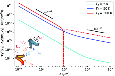
Figure 2: Torque on a particle due to fluctuating sources in a neighboring particle. Two objects can exchange net angular momentum amongst themselves and their environment, illustrated by an inset schematic. For concreteness, we plot $\bm{\tau}_{2}^{(1)}(T_{2})\cdot\mathbf{e}_{z}$, the torque on particle 1 due to the sources in particle 2, normalized by $\hbar V_{1}V_{2}$ where $V_{1}$ and $V_{2}$ are the volumes of particle 1 and 2, respectively, as a function of the separation $d$ along the $x$-direction of two InSb particles in the $xy$-plane subject to an external magnetic field in the $z$-direction. Solid/dashed lines indicate positive/negative values.

IV Concluding Remarks

In summary, we have introduced trace expressions for non-equilibrium Casimir torque that apply to arbitrary object shapes and materials, generalizing prior work on power transfer Molesky et al. [2019a], Bimonte et al. [2017a], Venkataram et al. [2020a] and forces Bimonte et al. [2017a], Krüger et al. [2012], Venkataram et al. [2020b] and showing explicitly the need for a full account of the spin and orbital angular momentum carried by waves in this setting. Furthermore, we have shown that recently developed techniques Molesky et al. [2020b, c, 2022], Chao et al. [2022], Venkataram et al. [2020b, a] for calculating bounds on sesquilinear objectives in electromagnetics can be applied to torque problems, revealing volumetric scaling for small and large object asymptotics in a shape-independent framework. The closeness of the associated limits with specific body shapes as discovered by inverse design, continues a trend observed in previous works on bounds to thermal absorption and emission Molesky et al. [2020a, c]. Although the calculated bounds focused exclusively on contributions from a dominant frequency, extensions to net (spectrally integrated) torque can be carried out as described in Ref. Molesky et al. [2022]. Further extensions to analyze the impact of nonreciprocal and anisotropic media will also be considered in the near future.

Appendix A Thermal field correlations in equilibrium and non-equilibrium settings

In this section, we summarize the details of the use of fluctuation-dissipation theorem (FDT) and local equilibrium properties with the scattering equations as described in Refs. Bimonte et al. [2017a], Krüger et al. [2012], modified to SI units and without assumptions of reciprocity. Let $\langle\cdots\rangle_{T}$ denote an equilibrium thermal average at a temperature $T.$ In the Rytov formalism for fluctuation electrodynamics Rytov et al. [1989], one assumes that the free dipoles inside an object fluctuate. In thermal equilibrium, one can show that the fluctuation-dissipation theorem gives Novotny and Hecht [2012], Bimonte et al. [2017a],

$$\underbrace{\left\langle J_{i}(\mathbf{x},\omega)J_{j}^{*}(\mathbf{x}^{\prime},\omega^{\prime})\right\rangle_{T}}_{\text{fluctuation}}=$$

$$\frac{\omega\epsilon_{0}}{2\pi}\coth\left(\frac{\hbar\omega}{2k_{B}T}\right)\underbrace{\bm{\chi}_{ij}^{\mathsf{A}}(\mathbf{x},\mathbf{x}^{\prime};\omega)}_{\text{dissipation}}\delta(\omega-\omega^{\prime}),$$ (28)

$$\mathbb{C}_{ij}^{eq}(T,\omega,\omega^{\prime};\mathbf{r},\mathbf{r}^{\prime}) \equiv\left\langle E_{i}(\mathbf{r},\omega)E_{j}^{*}(\mathbf{r}^{\prime},\omega^{\prime})\right\rangle_{T}$$ (29)

$$=b(T)\delta(\omega-\omega^{\prime})\mathbb{G}^{\mathsf{A}}_{ij}(\omega;\mathbf{r},\mathbf{r}^{\prime})$$ (30)

where

$$b(T)\equiv\frac{\hbar\omega^{2}}{2\pi c^{2}\epsilon_{0}}\coth\left(\frac{\hbar\omega}{2k_{B}T}\right).$$ (31)

One can also define

$$b(T) \equiv a(T)+a_{zp}$$ (32)

$$a(T) \equiv\text{sgn}(\omega)\frac{\hbar\omega^{2}}{\pi c^{2}\epsilon_{0}}\frac{1}{\exp\big(\frac{\hbar|\omega|}{k_{B}T}\big{missing})-1}$$ (33)

$$a_{zp} \equiv\text{sgn}(\omega)\frac{\hbar\omega^{2}}{2\pi c^{2}\epsilon_{0}}$$ (34)

to further break-up the terms into a temperature dependent piece and a quantum zero-point term. The Dyadic Green’s function satisfies

$$\left[\mathbb{H}_{0}-\mathbb{V}-\frac{\omega^{2}}{c^{2}}\mathbb{I}\right]\mathbb{G}(\mathbf{r},\mathbf{r}^{\prime})=\mathbb{I}\delta^{(3)}(\mathbf{r}-\mathbf{r}^{\prime}),$$ (35)

where $\mathbb{H}_{0}=\nabla\times\nabla\times$ and

$$\mathbb{V}=\frac{\omega^{2}}{c^{2}}(\mathbb{\epsilon}-\mathbb{I})+\nabla\times(\mathbb{I}-\mathbb{\mu}^{-1})\nabla\times.$$ (36)

The vacuum Green’s function $\mathbb{G}_{0}$ is the solution of Eq. (35) with $\mathbb{V}=0.$

Before considering non-equilibrium situations, rewrite the equilibrium expressions. As a first step, use the (mathematically trivial) fact that $\mathbb{G}^{\mathsf{A}}=-\mathbb{G}\mathbb{G}^{-1\mathsf{A}}\mathbb{G}^{\dagger}$ and the fact that, from Eq. (35),

$$-(\mathbb{G}^{-1}-\mathbb{G}_{0}^{-1})^{\mathsf{A}}=\mathbb{V}^{\mathsf{A}}.$$ (37)

This then lets one write

$$\mathbb{G}^{\mathsf{A}}=\mathbb{G}(\mathbb{V}^{\mathsf{A}}-\mathbb{G}_{0}^{-1\mathsf{A}})\mathbb{G}^{\dagger}$$ (38)

Suppose that there are $N$ objects labeled by $\alpha=1,\dots,N.$ Then one may rewrite the expression for $\mathbb{C}^{eq}$ to get

$$\mathbb{C}^{eq}(T)=\mathbb{C}^{zp}+\mathbb{C}^{env}(T)+\sum_{\alpha}\mathbb{C}_{\alpha}^{src}(T).$$ (39)

where $\mathbb{V}=\sum_{\alpha}\mathbb{V}_{\alpha}$ and

$$\mathbb{C}_{zp} =a_{zp}\mathbb{G}^{\mathsf{A}},$$ (40)

$$\mathbb{C}_{\alpha}^{src}(T) =a(T)\mathbb{G}\mathbb{V}_{\alpha}^{\mathsf{A}}\mathbb{G}^{\dagger},$$ (41)

$$\mathbb{C}_{env}(T) =-a(T)\mathbb{G}\mathbb{G}_{0}^{-1\mathsf{A}}\mathbb{G}^{\dagger}.$$ (42)

The interpretation is as follows. $\mathbb{C}_{\alpha}^{src}$, which involves $\mathbb{V}_{\alpha}$, is interpreted as the contribution to the spectral density function due to the sources in object $\alpha$, so that the “left-over” term $\mathbb{C}^{env}$ is interpreted as the contribution from the environment (which is anything not described by the non-zero parts of $\mathbb{V}$).

At this point, some assumptions have to be made in order to proceed further. We assume that in the non-equilibrium situation one may still use the above decomposition by assuming that the fluctuations still satisfy the fluctuation-dissipation theorem at the corresponding local temperatures of each object. Also, we assume that the time scales for temperature changes are much longer than the time scales for observation of the mechanical effects. Assuming that all the temperatures are independently tunable, the non-equilibrium expression for the field correlator becomes

$$\mathbb{C}^{neq}(T_{env},\{T_{\alpha}\}) =\mathbb{C}_{zp}+\mathbb{C}_{env}(T_{env})+\sum_{\alpha}\mathbb{C}_{\alpha}^{src}(T_{\alpha})$$ (43)

$$=\mathbb{C}^{eq}(T_{env})+\sum_{\alpha}[\mathbb{C}_{\alpha}^{src}(T_{\alpha})-\mathbb{C}_{\alpha}^{src}(T_{env})].$$ (44)

Suppose that there is only one body. Then

$$\mathbb{C}^{neq}(T_{env},T_{body}) =\mathbb{C}_{zp}+\mathbb{C}_{env}(T_{env})+\mathbb{C}_{body}^{src}(T_{body})$$ (45)

$$=\mathbb{C}^{eq}(T_{env})+(\mathbb{C}_{body}^{src}(T_{body})-\mathbb{C}_{body}^{src}(T_{env}))$$

where

$$\mathbb{C}_{env}(T_{env}) =-a(T_{env})\mathbb{G}_{body}\mathbb{G}_{0}^{-1\mathsf{A}}\mathbb{G}_{body}^{\dagger},$$ (46)

$$\mathbb{C}_{body}^{src}(T_{body}) =a(T_{body})\mathbb{G}_{body}\mathbb{V}_{body}^{\mathsf{A}}\mathbb{G}_{body}^{\dagger}.$$ (47)

We remark that it is possible to write the formulas using $\mathbb{G}$ directly, but we choose to rewrite the quantities using the $\mathbb{T}$ operator. The bounds are found by maximizing an objective function with respect to possible scattering operator response, making an objective in terms of scattering operators more useful than one in terms of the total Green’s function. This is done by rewriting, using $\mathbb{G}_{body}=\mathbb{G}_{0}+\mathbb{G}_{0}\mathbb{T}_{body}\mathbb{G}_{0}$, so that

$$\mathbb{C}_{env}(T_{env}) =-a(T_{env})\mathbb{G}_{body}\mathbb{G}_{0}^{-1\mathsf{A}}\mathbb{G}_{body}^{\dagger}$$

$$=a(T_{env})(\mathbb{I}+\mathbb{G}_{0}\mathbb{T}_{body})\mathbb{G}_{0}^{\mathsf{A}}(\mathbb{I}+\mathbb{T}_{body}^{\dagger}\mathbb{G}_{0}^{\dagger}).$$ (48)

$$\mathbb{C}_{body}^{src}(T_{body}) =a(T_{body})\mathbb{G}_{body}\mathbb{V}_{body}^{\mathsf{A}}\mathbb{G}_{body}^{\dagger}$$

$$=a(T_{body})\bigg{(}(\mathbb{G}_{0}+\mathbb{G}_{0}\mathbb{T}_{body}\mathbb{G}_{0})$$

$$\qquad\qquad\qquad\mathbb{V}_{body}^{\mathsf{A}}(\mathbb{G}_{0}+\mathbb{G}_{0}\mathbb{T}_{body}\mathbb{G}_{0})^{\dagger}\bigg{)}$$ (49)

While the above equations are true, they do not lead directly to trace formulas. For this to occur, one must be able to extend integrals over a particular region to that of the entire space. A way to do this is to write the expressions so that the $\mathbb{T}$ operator (or $\mathbb{V}$) appears on the right (or left) in integrands. Since the $\mathbb{T}$ vanishes unless both spatial arguments are inside $\mathbb{V}$, one may then extend the integral over all space, resulting in a trace expression. Multiplying Eq. (A) on the right by $\mathbb{G}_{0}^{-1\dagger}$ gives the correct form, but Eq. (A) does not. A way around this is to note that (ignoring $\delta(\omega-\omega^{\prime})$ factors)

$$\mathbb{C}_{body}^{src}(T)+\mathbb{C}_{env}(T) =a(T)\mathbb{G}_{body}^{\mathsf{A}}$$ (50)

$$=a(T)(\mathbb{G}_{0}+\mathbb{G}_{0}\mathbb{T}_{body}\mathbb{G}_{0})^{\mathsf{A}},$$ (51)

which along with Eq. (A) gives, after a few lines of algebraic manipulations,

$$\mathbb{C}_{body}^{src}(T) =a(T)\mathbb{G}_{0}\left(\mathbb{T}_{body}^{\mathsf{A}}-\mathbb{T}_{body}\mathbb{G}_{0}^{\mathsf{A}}\mathbb{T}_{body}^{\dagger}\right)\mathbb{G}_{0}^{\dagger},$$ (52)

$$\equiv a(T)\mathbb{R}_{body},$$ (53)

where in the last line we defined the radiation operator $\mathbb{R}_{body},$ so called as it appears in formulas involving a surface integral of the Poynting vector Krüger et al. [2012]. Note that this required that $\mathbb{C}_{env}$ and $\mathbb{C}_{body}^{src}$ be evaluated at the same temperatures. This is where the utility of the second line of Eq. (45) becomes apparent. Note also that $\mathbb{C}_{body}^{src}\mathbb{G}_{0}^{-1\dagger}$ has a right-most $\mathbb{T}_{body}$ operator, so that spatial integrals over the body $\int_{V_{body}}d\mathbf{r}(\dots)$ can be extended over all space if the integrand depends on $\mathbb{C}_{body}^{src}\mathbb{G}_{0}^{-1\dagger},$ which it does for power and force Krüger et al. [2012] as well as for torque (see Eq. (14)). The non-equilibrium portion of heat transfer, forces, and torques depends solely on $(\mathbb{C}_{body}^{src}(T_{body})-\mathbb{C}_{body}^{src}(T_{env}))$.

Appendix B Evaluation of Green’s function in spherical domains

Once an origin has been specified, the Green’s function can be expanded in terms of the regular spherical vector waves $\mathbf{RN},\mathbf{RM}$ and in terms of the outgoing spherical vector waves $\mathbf{N},\mathbf{M}$ as  Tsang et al. [2004]

$$\mathbb{G}_{0}(\mathbf{x},\mathbf{y})=-\frac{\delta(\mathbf{x}-\mathbf{y})}{k^{2}}\hat{x}\otimes\hat{y}+ik\sum_{J=1}^{\infty}\sum_{M=-J}^{J}(-1)^{M}$$ (54)

$$\begin{cases}\mathbf{M}_{J,M}(k\mathbf{x})\mathbf{RM}_{J,-M}(k\mathbf{y})+\mathbf{N}_{J,M}(k\mathbf{x})\mathbf{RN}_{J,-M}(k\mathbf{y}),x>y\\ \mathbf{RM}_{J,M}(k\mathbf{x})\mathbf{M}_{J,-M}(k\mathbf{y})+\mathbf{RN}_{J,M}(k\mathbf{x})\mathbf{N}_{J,-M}(k\mathbf{y}),x<y\end{cases}$$

The asymmetric part has a spectral basis expansion as

$$\mathbb{G}_{0}^{\mathsf{A}}(\mathbf{x},\mathbf{y})=k\sum_{J,M}(-1)^{M}\Bigg{(}\mathbf{RM}_{J,M}(k\mathbf{x})\mathbf{RM}_{J,-M}(k\mathbf{y})+$$

$$\mathbf{RN}_{J,M}(k\mathbf{x})\mathbf{RN}_{J,-M}(k\mathbf{y})\Bigg{)}$$ (55)

Explicitly,

$$\mathbf{RN}_{J,M}(\mathbf{y}) =\frac{\sqrt{J(J+1)}}{y}j_{J}(y)\mathbf{A}_{JM}^{(3)}+\frac{1}{y}\frac{\partial(yj_{J}(y))}{\partial y}\mathbf{A}_{JM}^{(2)}$$ (56)

$$\mathbf{RM}_{J,M}(\mathbf{y}) =j_{J}(y)\mathbf{A}_{JM}^{(1)}$$ (57)

$$\mathbf{N}_{J,M}(\mathbf{y}) =\frac{\sqrt{J(J+1)}}{y}h_{J}^{(1)}(y)\mathbf{A}_{JM}^{(3)}+\frac{1}{y}\frac{\partial(yh_{J}^{(1)}(y))}{\partial y}\mathbf{A}_{JM}^{(2)}$$ (58)

$$\mathbf{M}_{J,M}(\mathbf{y}) =h_{J}^{(1)}(y)\mathbf{A}_{JM}^{(1)}$$ (59)

where $j_{J}(y)$ is the spherical Bessel function of order $J$ and $h_{J}^{(1)}(y)$ is the spherical Hankel function of order $J.$

$$\mathbf{A}_{JM}^{(1)}(\hat{\mathbf{r}}) =\frac{1}{\sqrt{J(J+1)}}\nabla\times(\mathbf{r}Y_{JM}(\hat{\mathbf{r}}))$$

$$=\frac{1}{\sqrt{J(J+1)}}\nabla Y_{JM}(\hat{\mathbf{r}})\times\mathbf{r}$$ (60)

$$\mathbf{A}_{JM}^{(2)}(\hat{\mathbf{r}}) =\frac{1}{\sqrt{J(J+1)}}r\nabla Y_{JM}(\hat{\mathbf{r}})$$ (61)

$$\mathbf{A}_{JM}^{(3)}(\hat{\mathbf{r}}) =\hat{\mathbf{r}}Y_{JM}(\hat{\mathbf{r}})$$ (62)

and the convention is such that

$$Y_{JM}(\theta,\phi)=\sqrt{\frac{2J+1}{4\pi}\frac{(J-M)!}{(J+M)!}}P_{J}^{M}(\text{cos}\left(\theta\right))e^{im\phi}$$ (63)

where $P_{J}^{M}(z)$ is the associated Legendre polynomial. The eigenvalues of $\mathbb{G}_{0}^{\mathsf{A}}$ are Molesky et al. [2019a]

$$\rho_{RM,J,M} =\frac{\pi(kR)^{2}}{4k^{2}}\left(J_{J+\frac{1}{2}}^{2}(kR)-J_{J-\frac{1}{2}}(kR)J_{J+\frac{3}{2}}(kR)\right)$$ (64)

$$\rho_{RN,J,M} =\frac{\pi(kR)^{2}}{4k^{2}}\Bigg{(}\frac{J+1}{2J+1}\bigg{(}J_{J-\frac{1}{2}}^{2}(kR)$$

$$-J_{J+\frac{1}{2}}(kR)J_{J-\frac{3}{2}}(kR)\bigg{)}+$$

$$\frac{J}{2J+1}\left(J_{J+\frac{3}{2}}^{2}(kR)-J_{J+\frac{1}{2}}(kR)J_{J+\frac{5}{2}}(kR)\right)\Bigg{)}$$ (65)

where $J_{\nu}$ is a Bessel function of the first kind of order $\nu.$

Note that $-i\frac{\partial}{\partial\phi}$ acting on the vector spherical harmonics does not simply introduce an overall factor of $m.$ This is because the coordinate vectors $\mathbf{e}_{r},\mathbf{e}_{\theta},\mathbf{e}_{\phi}$ depend on $\phi$ as well. More to the point, $-i\frac{\partial}{\partial\phi}=\hat{L}_{z}$ (math references usually have $\hbar=1$) in the position space representation but the vector spherical harmonics are not defined to be eigenstates of $\hat{L}_{z}.$ That said, there does exist an operator, let us call it $\hat{J}_{z}$, equal to $\hat{J}_{z}=\hat{L}_{z}+\hat{S}_{z}$ for some operator $\hat{S}_{z}$ that cancels the terms introduced by the action of $\frac{\partial}{\partial\phi}$ on $\mathbf{e}_{r},\mathbf{e}_{\theta},\mathbf{e}_{\phi}$ such that the vector spherical harmonics are eigenfunctions of $\hat{J}_{z}$ with eigenvalues equal to the $m$ label. See Section C for more details.

Appendix C Tensor spherical harmonics

In this section, we summarize several salient mathematical identities and definitions from Ref. Khersonskii et al. surrounding tensor spherical harmonics. The tensor spherical harmonics $Y_{JM}^{LS}(\theta,\phi)$ are, by definition, eigenfunctions of the operators $\hat{\mathbf{J}}^{2},\hat{J}_{z},\hat{\mathbf{L}}^{2},$ and $\hat{\mathbf{S}}^{2}$ where $\hat{\mathbf{L}}$ is the operator for the orbital angular momentum, $\hat{\mathbf{S}}$ is the operator for the spin, and $\hat{\mathbf{J}}=\hat{\mathbf{L}}+\hat{\mathbf{S}}$ is the operator for the total angular momentum. Explicitly,

$$\hat{\mathbf{J}}^{2}Y_{JM}^{LS}(\theta,\phi) =J(J+1)Y_{JM}^{LS}(\theta,\phi)$$ (66)

$$\hat{J_{z}}Y_{JM}^{LS}(\theta,\phi) =MY_{JM}^{LS}(\theta,\phi)$$ (67)

$$\hat{\mathbf{L}}^{2}Y_{JM}^{LS}(\theta,\phi) =L(L+1)Y_{JM}^{LS}(\theta,\phi)$$ (68)

$$\hat{\mathbf{S}}^{2}Y_{JM}^{LS}(\theta,\phi) =S(S+1)Y_{JM}^{LS}(\theta,\phi).$$ (69)

Note that the units are such that $\hbar=1.$ The interpretation within physics is that the tensor spherical harmonics may be used in the expansion of the angular distribution and polarization of spin-$S$ particles. The tensor spherical harmonics are states with definite total angular momentum $J$, definite projection $M$ along an axis (chosen to be the $z$ axis), and definite orbital angular momentum $L.$ For $S=0,$ these are just the spherical harmonics, often written $Y_{lm}(\theta,\phi)$ or $Y_{l}^{m}(\theta,\phi).$ The $S=\frac{1}{2}$ functions are sometimes called spinor spherical harmonics. The $S=1$ states are the vector spherical harmonics, etc. (The transformation properties of the tensor spherical harmonics under a rotation of the coordinate system are determined by $J,$ and not $L$ or $S$ so calling them spinor or vector spherical harmonics is a bit of a misnomer from this point of view.)

The tensor spherical harmonics may be constructed from the spherical harmonics, let us label them $Y_{LM}(\theta,\phi)$ (instead of $Y_{lm}(\theta,\phi)$ of $Y_{l}^{m}(\theta,\phi)).$ The expansion is

$$Y_{JM}^{LS}(\theta,\phi)=\sum_{M,\sigma}C_{LMS\sigma}^{JM}Y_{LM}(\theta,\phi)\chi_{S\sigma}.$$ (70)

This follows from the fact that any total angular momentum basis $\ket{jm;l\sigma}$ can be expanded in terms of the direct product basis $\ket{lm_{l};\sigma m_{\sigma}}\equiv\ket{lm_{l}}\otimes\ket{\sigma m_{\sigma}}$ and the Clebsch-Gordon coefficients

$$\ket{jm;l\sigma}=\sum_{m_{l}=-l}^{l}\sum_{m_{\sigma}=-\sigma}^{\sigma}\innerproduct{lm_{l};\sigma m_{\sigma}}{jm;l\sigma}\ket{lm_{l};\sigma m_{\sigma}}$$ (71)

In the coordinate representation $\hat{\mathbf{L}}$ is represented as a differential operator $\hat{\mathbf{L}}=-i\mathbf{r}\times\nabla.$ Using the coordinate representation and the fact that, by definition, the spherical harmonics $Y_{lm}(\theta,\phi)$ satisfy

$$\hat{\mathbf{L}}^{2}Y_{lm}(\theta,\phi) =l(l+1)Y_{lm}(\theta,\phi)$$ (72)

$$\hat{L}_{z}Y_{lm}(\theta,\phi) =mY_{lm}(\theta,\phi)$$ (73)

gives the coordinate representation claimed in Eq. (70). The indices $J$ and $S$ are integer or half-integer nonnegative numbers. $L$ is a nonnegative integer. For a fixed value of $J$ and $S,$ then $L$ can only take on values from $|J-S|,|J-S|+1,\dots,J+S-1,J+S.$ For a given value of $J,$ then $M$ can only take on values from $-J,-J+1,\dots,J-1,J.$

For fixed values of $J,M,L,S$ the tensor spherical harmonics are function of $\theta,\phi,$ and $\xi,$ where $\xi$ is the spin variable. The polar angles are $\theta,\phi$ take on values $0\leq\theta\leq\pi$ and $0\leq\phi\leq 2\pi.$ To be precise, one should write $Y_{JM}^{LS}(\theta,\phi,\xi)$ but the dependence on the spin variable is usually not explicitly mentioned. The reason for this is because of the next step: Represent $Y_{JM}^{LS}(\theta,\phi)$ as a column matrix (that is, a column vector) of length $2S+1.$ Therefore, the spin variable now refers to a particular component of the column vector, and summation of spin variables has the interpretation of matrix multiplication. Using the matrix notation, the following orthogonality relation holds:

$$\sum_{M}(Y_{LM}^{L^{\prime},S}(\theta,\phi))^{*T}\cdot Y_{JM}^{LS}(\theta,\phi)=0,\text{ if }L^{\prime}\neq L.$$ (74)

C.1 Vector spherical harmonics

The vector spherical harmonics are defined as the tensor spherical harmonics with $S=1;$ they are $Y_{JM}^{L,1}(\theta,\phi).$ Using the vector notation,

$$Y_{JM}^{L,1}(\theta,\phi)=\sum_{M,\sigma}C_{LM1\sigma}^{JM}Y_{LM}(\theta,\phi)\mathbf{e}_{\sigma},$$ (75)

where $\mathbf{e}_{\sigma}$ are a covariant spherical basis vector. That is,

$$\mathbf{e}_{+1} =-\frac{1}{\sqrt{2}}(\mathbf{e}_{x}+i\mathbf{e}_{y}),$$ (76a)

$$\mathbf{e}_{0} =\mathbf{e}_{z},$$ (76b)

$$\mathbf{e}_{-1} =\frac{1}{\sqrt{2}}(\mathbf{e}_{x}-i\mathbf{e}_{y}).$$ (76c)

For a fixed value of $J,$ the possible values of $L$ are $J-1,J,J+1,$ with the exception of $J=0,$ where only $L=1$ is allowed.

While the covariant spherical basis vectors are nice from a mathematical theoretical point of view and lead to cleaner transformation properties of their components under rotations of coordinate systems, other bases are possible. The change of basis formulas from covariant spherical basis to Cartesian or polar coordinates are straightforward (see below).

Given this introduction to tensor spherical harmonics, a valid question is how does this relate to $\mathbf{A}_{JM}^{(1)},\mathbf{A}_{JM}^{(2)},\mathbf{A}_{JM}^{(3)}$ which are also called vector spherical harmonics. Note that $Y_{JM}^{LS}$ are, by definition, states of definite orbital angular momentum. In the context of radiation settings in electromagnetism, it can be convenient to work in a basis that separates longitudinal and transverse waves. It turns out that

$$\mathbf{A}_{JM}^{(1)}(\hat{\mathbf{r}}) =-iY_{JM}^{J,1}(\theta,\phi),$$ (77)

$$\mathbf{A}_{JM}^{(2)}(\hat{\mathbf{r}}) =\sqrt{\frac{J+1}{2J+1}}Y_{JM}^{J-1,1}(\theta,\phi)+\sqrt{\frac{J}{2J+1}}Y_{JM}^{J+1,1}(\theta,\phi),$$ (78)

$$\mathbf{A}_{JM}^{(3)}(\hat{\mathbf{r}}) =\sqrt{\frac{J}{2J+1}}Y_{JM}^{J-1,1}(\theta,\phi)-\sqrt{\frac{J+1}{2J+1}}Y_{JM}^{J+1,1}(\theta,\phi)$$ (79)

are the needed combinations of the tensor spherical harmonics (up to overall constant complex factors) for the decomposition into transverse and longitudinal waves. $\mathbf{A}_{JM}^{(3)}$ are longitudinal waves. $\mathbf{A}_{JM}^{(1)}$ and $\mathbf{A}_{JM}^{(2)}$ are transverse waves, sometimes called magnetic and electric multipoles, respectively. See Chapter 7 of Ref. Khersonskii et al. for more details. Ref. Dai et al. [2012] explicitly works out the divergence of the tensor spherical waves and shows how to use the expressions for the divergence to construct linear combinations of the tensor spherical waves that are longitudinal and transverse. This process is invertible, namely,

$$Y_{JM}^{J,1}(\theta,\phi) =i\mathbf{A}_{JM}^{(1)}(\hat{\mathbf{r}}),$$ (80)

$$Y_{J,M}^{J+1,1}(\theta,\phi) =\sqrt{\frac{J}{2J+1}}\mathbf{A}_{JM}^{(2)}(\hat{\mathbf{r}})-\sqrt{\frac{J+1}{2J+1}}\mathbf{A}_{JM}^{(3)}(\hat{\mathbf{r}}),$$ (81)

$$Y_{JM}^{J-1,1}(\theta,\phi) =\sqrt{\frac{J+1}{2J+1}}\mathbf{A}_{JM}^{(2)}(\hat{\mathbf{r}})+\sqrt{\frac{J}{2J+1}}\mathbf{A}_{JM}^{(3)}(\hat{\mathbf{r}})$$ (82)

so $\mathbf{A}_{JM}^{(1)},\mathbf{A}_{JM}^{(2)},\mathbf{A}_{JM}^{(3)}$ also constitute a complete orthonormal vector set for the range $0\leq\theta\leq\pi,$ $0\leq\phi\leq 2\pi.$ Their longitudinal and transverse orientations relative to $\hat{\mathbf{r}}$ makes them a convenient basis to use in radiation settings in electromagnetism.

C.2 The $\hat{S}_{z}$ Operator

In the covariant spherical basis Khersonskii et al. ,

$$\hat{S}_{z}=\begin{bmatrix}1&0&0\\ 0&0&0\\ 0&0&-1\end{bmatrix}.$$ (83)

From Eq. (76), it follows that the change-of-basis operator from $\{\mathbf{e}_{+1},\mathbf{e}_{0},\mathbf{e}_{-1}\}$ to $\{\mathbf{e}_{x},\mathbf{e}_{y},\mathbf{e}_{z}\}$ is

$$M(x,y,z\leftarrow+1,0,-1)=\begin{bmatrix}-\frac{1}{\sqrt{2}}&0&\frac{1}{\sqrt{2}}\\ -\frac{i}{\sqrt{2}}&0&-\frac{i}{\sqrt{2}}\\ 0&1&0\end{bmatrix}.$$ (84)

Likewise, the change-of-basis operator from $\{\mathbf{e}_{+1},\mathbf{e}_{0},\mathbf{e}_{-1}\}$ to $\{\mathbf{e}_{r},\mathbf{e}_{\theta},\mathbf{e}_{\phi}\}$ is

$$M(r,\theta,\phi\leftarrow+1,0,-1)=\begin{bmatrix}-\frac{\text{sin}\left(\theta\right)}{\sqrt{2}}e^{i\phi}&\text{cos}\left(\theta\right)&\frac{\text{sin}\left(\theta\right)}{\sqrt{2}}e^{-i\phi}\\ -\frac{\text{cos}\left(\theta\right)}{\sqrt{2}}e^{i\phi}&-\text{sin}\left(\theta\right)&\frac{\text{cos}\left(\theta\right)}{\sqrt{2}}e^{-i\phi}\\ -\frac{i}{\sqrt{2}}e^{i\phi}&0&-\frac{i}{\sqrt{2}}e^{-i\phi}\end{bmatrix}.$$ (85)

It follows that in the polar coordinate basis $\{\mathbf{e}_{r},\mathbf{e}_{\theta},\mathbf{e}_{\phi}\}$

$$\hat{S}_{z}=\begin{bmatrix}0&0&-i\text{sin}\left(\theta\right)\\ 0&0&-i\text{cos}\left(\theta\right)\\ i\text{sin}\left(\theta\right)&i\text{cos}\left(\theta\right)&0\end{bmatrix}.$$ (86)

From these change-of-basis operators, it follows that in the Cartesian coordinate basis $\{\mathbf{e}_{x},\mathbf{e}_{y},\mathbf{e}_{z}\}$

$$\hat{S}_{z}=\begin{bmatrix}0&-i&0\\ i&0&0\\ 0&0&0\end{bmatrix}.$$ (87)

C.3 Action of $\hat{L}_{z}$ and $\hat{S}_{z}$ on $Y_{JM}^{LS}$

Let $\Phi(r)$ be an arbitrary function of $r=|\mathbf{r}|.$ From Ref. Khersonskii et al. , the following holds:

$$\hat{L}_{\mu}\{\Phi(r)Y_{JM}^{LS}(\theta,\phi)\} =\Phi(r)\hat{L}_{\mu}\{Y_{JM}^{LS}(\theta,\phi)\}$$

$$=(-1)^{J+L+S+1}\Phi(r)\sqrt{(2J+1)L(L+1)(2L+1)}\sum_{J^{\prime}}\begin{Bmatrix}J&J^{\prime}&1\\ L&L&S\end{Bmatrix}C_{JM1\mu}^{J^{\prime}M+\mu}Y_{J^{\prime}M+\mu}^{LS}(\theta,\phi).$$ (88)

$$\hat{S}_{\mu}\{\Phi(r)Y_{JM}^{LS}(\theta,\phi)\} =\Phi(r)\hat{S}_{\mu}\{Y_{JM}^{LS}(\theta,\phi)\}$$

$$=(-1)^{L+1}\Phi(r)\sqrt{(2J+1)S(S+1)(2S+1)}\sum_{J^{\prime}}(-1)^{J^{\prime}+S}\begin{Bmatrix}J&J^{\prime}&1\\ S&S&L\end{Bmatrix}C_{JM1\mu}^{J^{\prime}M+\mu}Y_{J^{\prime}M+\mu}^{LS}(\theta,\phi).$$ (89)

When $\mu=0,$ the spherical coordinate components are equal to the Cartesian coordinate components. Namely,

$$\hat{L}_{z}\{\Phi(r)Y_{JM}^{LS}(\theta,\phi)\} =\Phi(r)\hat{L}_{z}\{Y_{JM}^{LS}(\theta,\phi)\}$$

$$=(-1)^{J+L+S+1}\Phi(r)\sqrt{(2J+1)L(L+1)(2L+1)}\sum_{J^{\prime}}\begin{Bmatrix}J&J^{\prime}&1\\ L&L&S\end{Bmatrix}C_{JM10}^{J^{\prime}M}Y_{J^{\prime}M}^{LS}(\theta,\phi).$$ (90)

$$\hat{S}_{z}\{\Phi(r)Y_{JM}^{LS}(\theta,\phi)\} =\Phi(r)\hat{S}_{z}\{Y_{JM}^{LS}(\theta,\phi)\}$$

$$=(-1)^{L+1}\Phi(r)\sqrt{(2J+1)S(S+1)(2S+1)}\sum_{J^{\prime}}(-1)^{J^{\prime}+S}\begin{Bmatrix}J&J^{\prime}&1\\ S&S&L\end{Bmatrix}C_{JM10}^{J^{\prime}M}Y_{J^{\prime}M}^{LS}(\theta,\phi).$$ (91)

C.4 Action of $\hat{S}_{z}$ on $\mathbf{A}_{JM}^{(1)},\mathbf{A}_{JM}^{(2)},\mathbf{A}_{JM}^{(3)}$

Using the results of the previous parts,

$$\hat{S}_{z}\mathbf{A}_{JM}^{(1)} =-i(-1)^{J+1}\sqrt{(2J+1)S(S+1)(2S+1)}\sum_{J^{\prime}}(-1)^{J^{\prime}+1}\begin{Bmatrix}J&J^{\prime}&1\\ 1&1&J\end{Bmatrix}C_{JM10}^{J^{\prime}M}Y_{J^{\prime}M}^{J,1}$$ (92)

$$=-i(-1)^{J+1}\sqrt{(2J+1)S(S+1)(2S+1)}\bigg{(}(-1)^{J}\begin{Bmatrix}J&J-1&1\\ 1&1&J\end{Bmatrix}C^{J-1,M}_{JM10}Y^{J,1}_{J-1,M}$$

$$+(-1)^{J+1}\begin{Bmatrix}J&J&1\\ 1&1&J\end{Bmatrix}C^{J,M}_{JM10}Y^{J,1}_{J,M}$$

$$+(-1)^{J}\begin{Bmatrix}J&J+1&1\\ 1&1&J\end{Bmatrix}C^{J+1,M}_{JM10}Y^{J,1}_{J+1,M}\bigg{)}$$

$$=-i(-1)^{J+1}\sqrt{(2J+1)S(S+1)(2S+1)}\bigg{(}$$

$$(-1)^{J}\begin{Bmatrix}J&J-1&1\\ 1&1&J\end{Bmatrix}C^{J-1,M}_{JM10}\sqrt{\frac{J-1}{2J-1}}\mathbf{A}_{J-1,M}^{(2)}-(-1)^{J}\begin{Bmatrix}J&J-1&1\\ 1&1&J\end{Bmatrix}C^{J-1,M}_{JM10}\sqrt{\frac{J}{2J-1}}\mathbf{A}_{J-1,M}^{(3)}$$

$$+(-1)^{J+1}\begin{Bmatrix}J&J&1\\ 1&1&J\end{Bmatrix}C^{J,M}_{JM10}i\mathbf{A}_{JM}^{(1)}$$

$$+(-1)^{J}\begin{Bmatrix}J&J+1&1\\ 1&1&J\end{Bmatrix}C^{J+1,M}_{JM10}\sqrt{\frac{J+2}{2J+3}}\mathbf{A}_{J+1,M}^{(2)}+(-1)^{J}\begin{Bmatrix}J&J+1&1\\ 1&1&J\end{Bmatrix}C^{J+1,M}_{JM10}\sqrt{\frac{J+1}{2J+3}}\mathbf{A}_{J+1,M}^{(3)}\bigg{)}$$

$$\hat{S}_{z}\mathbf{A}_{JM}^{(2)} =\sqrt{\frac{J+1}{2J+1}}(-1)^{J}\sqrt{(2J+1)S(S+1)(2S+1)}\sum_{J^{\prime}}(-1)^{J^{\prime}+1}\begin{Bmatrix}J&J^{\prime}&1\\ 1&1&J-1\end{Bmatrix}C_{JM10}^{J^{\prime}M}Y_{J^{\prime}M}^{J-1,1}$$ (93)

$$+\sqrt{\frac{J}{2J+1}}(-1)^{J}\sqrt{(2J+1)S(S+1)(2S+1)}\sum_{J^{\prime}}(-1)^{J^{\prime}+1}\begin{Bmatrix}J&J^{\prime}&1\\ 1&1&J+1\end{Bmatrix}C_{JM10}^{J^{\prime}M}Y_{J^{\prime}M}^{J+1,1}$$

$$=(-1)^{J}\sqrt{\frac{J+1}{2J+1}}\sqrt{(2J+1)S(S+1)(2S+1)}\bigg{(}$$

$$(-1)^{J}\begin{Bmatrix}J&J-1&1\\ 1&1&J-1\end{Bmatrix}C^{J-1,M}_{JM10}Y^{J-1,1}_{J-1,M}$$

$$+(-1)^{J+1}\begin{Bmatrix}J&J&1\\ 1&1&J-1\end{Bmatrix}C^{J,M}_{JM10}Y^{J-1,1}_{J,M}\bigg{)}$$

$$+(-1)^{J}\sqrt{\frac{J}{2J+1}}\sqrt{(2J+1)S(S+1)(2S+1)}\bigg{(}$$

$$(-1)^{J+1}\begin{Bmatrix}J&J&1\\ 1&1&J+1\end{Bmatrix}C_{JM10}^{J,M}Y_{JM}^{J+1,1}$$

$$+(-1)^{J}\begin{Bmatrix}J&J+1&1\\ 1&1&J+1\end{Bmatrix}C_{JM10}^{J+1,M}Y_{J+1,M}^{J+1,1}\bigg{)}$$

$$=(-1)^{J}\sqrt{\frac{J+1}{2J+1}}\sqrt{(2J+1)S(S+1)(2S+1)}\bigg{(}$$

$$(-1)^{J}\begin{Bmatrix}J&J-1&1\\ 1&1&J-1\end{Bmatrix}C^{J-1,M}_{JM10}i\mathbf{A}_{J-1,M}^{(1)}$$

$$+(-1)^{J+1}\begin{Bmatrix}J&J&1\\ 1&1&J-1\end{Bmatrix}C^{J,M}_{JM10}\sqrt{\frac{J+1}{2J+1}}\mathbf{A}_{J,M}^{(2)}+(-1)^{J+1}\begin{Bmatrix}J&J&1\\ 1&1&J-1\end{Bmatrix}C^{J,M}_{JM10}\sqrt{\frac{J}{2J+1}}\mathbf{A}_{J,M}^{(3)}\bigg{)}$$

$$+(-1)^{J}\sqrt{\frac{J}{2J+1}}\sqrt{(2J+1)S(S+1)(2S+1)}\bigg{(}$$

$$(-1)^{J+1}\begin{Bmatrix}J&J&1\\ 1&1&J+1\end{Bmatrix}C_{JM10}^{J,M}\sqrt{\frac{J}{2J+1}}\mathbf{A}_{JM}^{(2)}-(-1)^{J+1}\begin{Bmatrix}J&J&1\\ 1&1&J+1\end{Bmatrix}C_{JM10}^{J,M}\sqrt{\frac{J+1}{2J+1}}\mathbf{A}_{JM}^{(3)}$$

$$+(-1)^{J}\begin{Bmatrix}J&J+1&1\\ 1&1&J+1\end{Bmatrix}C_{JM10}^{J+1,M}i\mathbf{A}_{J+1,M}^{(1)}\bigg{)}$$

$$\hat{S}_{z}\mathbf{A}_{JM}^{(3)} =\sqrt{\frac{J}{2J+1}}(-1)^{J}\sqrt{(2J+1)S(S+1)(2S+1)}\sum_{J^{\prime}}(-1)^{J^{\prime}+1}\begin{Bmatrix}J&J^{\prime}&1\\ 1&1&J-1\end{Bmatrix}C_{JM10}^{J^{\prime}M}Y_{J^{\prime}M}^{J-1,1}$$ (94)

$$-\sqrt{\frac{J+1}{2J+1}}(-1)^{J}\sqrt{(2J+1)S(S+1)(2S+1)}\sum_{J^{\prime}}(-1)^{J^{\prime}+1}\begin{Bmatrix}J&J^{\prime}&1\\ 1&1&J+1\end{Bmatrix}C_{JM10}^{J^{\prime}M}Y_{J^{\prime}M}^{J+1,1}$$

$$=(-1)^{J}\sqrt{\frac{J}{2J+1}}\sqrt{(2J+1)S(S+1)(2S+1)}\bigg{(}$$

$$(-1)^{J}\begin{Bmatrix}J&J-1&1\\ 1&1&J-1\end{Bmatrix}C^{J-1,M}_{JM10}Y^{J-1,1}_{J-1,M}$$

$$+(-1)^{J+1}\begin{Bmatrix}J&J&1\\ 1&1&J-1\end{Bmatrix}C^{J,M}_{JM10}Y^{J-1,1}_{J,M}\bigg{)}$$

$$-(-1)^{J}\sqrt{\frac{J+1}{2J+1}}\sqrt{(2J+1)S(S+1)(2S+1)}\bigg{(}$$

$$(-1)^{J+1}\begin{Bmatrix}J&J&1\\ 1&1&J+1\end{Bmatrix}C_{JM10}^{J,M}Y_{JM}^{J+1,1}$$

$$+(-1)^{J}\begin{Bmatrix}J&J+1&1\\ 1&1&J+1\end{Bmatrix}C_{JM10}^{J+1,M}Y_{J+1,M}^{J+1,1}\bigg{)}$$

$$=(-1)^{J}\sqrt{\frac{J}{2J+1}}\sqrt{(2J+1)S(S+1)(2S+1)}\bigg{(}$$

$$(-1)^{J}\begin{Bmatrix}J&J-1&1\\ 1&1&J-1\end{Bmatrix}C^{J-1,M}_{JM10}i\mathbf{A}_{J-1,M}^{(1)}$$

$$+(-1)^{J+1}\begin{Bmatrix}J&J&1\\ 1&1&J-1\end{Bmatrix}C^{J,M}_{JM10}\sqrt{\frac{J+1}{2J+1}}\mathbf{A}_{J,M}^{(2)}+(-1)^{J+1}\begin{Bmatrix}J&J&1\\ 1&1&J-1\end{Bmatrix}C^{J,M}_{JM10}\sqrt{\frac{J}{2J+1}}\mathbf{A}_{J,M}^{(3)}\bigg{)}$$

$$-(-1)^{J}\sqrt{\frac{J+1}{2J+1}}\sqrt{(2J+1)S(S+1)(2S+1)}\bigg{(}$$

$$(-1)^{J+1}\begin{Bmatrix}J&J&1\\ 1&1&J+1\end{Bmatrix}C_{JM10}^{J,M}\sqrt{\frac{J}{2J+1}}\mathbf{A}_{JM}^{(2)}-(-1)^{J+1}\begin{Bmatrix}J&J&1\\ 1&1&J+1\end{Bmatrix}C_{JM10}^{J,M}\sqrt{\frac{J+1}{2J+1}}\mathbf{A}_{JM}^{(3)}$$

$$+(-1)^{J}\begin{Bmatrix}J&J+1&1\\ 1&1&J+1\end{Bmatrix}C_{JM10}^{J+1,M}i\mathbf{A}_{J+1,M}^{(1)}\bigg{)}$$

Analogous expressions for the action of $\hat{L}_{z}$ on $\mathbf{A}_{JM}^{(1)},\mathbf{A}_{JM}^{(2)},\mathbf{A}_{JM}^{(3)}$ can be derived starting from Eq. (90) and following steps similar to the above work. One can also start from $\hat{L}_{z}\mathbf{A}_{JM}=\hat{J}_{z}\mathbf{A}_{JM}-\hat{S}_{z}\mathbf{A}_{JM}=M\mathbf{A}_{JM}-\hat{S}_{z}\mathbf{A}_{JM}$ and then use the expressions just derived.

Appendix D Contibutions to $\Phi_{J}$ in the small $R$ limit

Let $R$ be a measure of the size of the compact body. In this section, we show that in the small $R$ limit the contributions from the $\hat{L}_{z}$ terms vanish exactly to lowest order in $R$ whereas they do not, in general, vanish from the $\hat{S}_{z}$ terms. This supports the intuitive semi-classical picture that the spin contributions dominate in the quasistatic regime. In the small $R$ limit, the $\mathbf{RN}_{JM}$ with $J=1$ terms dominate in $\Phi_{J}.$ In this limit (using $\lim_{x\to 0}\frac{\partial(xj_{J}(x))}{\partial x}\approx(J+1)j_{J}(x)$) one finds

$$\hat{J}_{z}\mathbb{G}_{0}^{\mathsf{A}}(\mathbf{x},\mathbf{y}) \approx\sum_{M=-1,0,1}M\mathbf{RN}_{1,M}(\mathbf{x})\mathbf{RN}_{1,M}^{*}(\mathbf{y})$$ (95)

$$\approx\sum_{M=-1,0,1}\frac{j_{1}(x)j_{1}(y)}{xy}\begin{bmatrix}\mathbf{A}_{1M}^{(1)}(\mathbf{x})\\ \mathbf{A}_{1M}^{(2)}(\mathbf{x})\\ \mathbf{A}_{1M}^{(3)}(\mathbf{x})\end{bmatrix}^{T}\mathcal{A}_{M}\begin{bmatrix}\mathbf{A}_{1M}^{(1)*}(\mathbf{y})\\ \mathbf{A}_{1M}^{(2)*}(\mathbf{y})\\ \mathbf{A}_{1M}^{(3)*}(\mathbf{y})\end{bmatrix}$$ (96)

where

$$\mathcal{A}_{-1}=\begin{bmatrix}0&0&0\\ 0&-4&-2\sqrt{2}\\ 0&-2\sqrt{2}&-2\end{bmatrix},\quad\mathcal{A}_{0}=\begin{bmatrix}0&0&0\\ 0&0&0\\ 0&0&0\end{bmatrix},\quad\mathcal{A}_{1}=\begin{bmatrix}0&0&0\\ 0&4&2\sqrt{2}\\ 0&2\sqrt{2}&2\end{bmatrix}.$$ (97)

In this small $R$ limit, $\Phi_{J}\approx-\frac{2}{\pi}\text{Tr}[\hat{J}_{z}\mathbb{G}_{0}^{\mathsf{A}}\mathbb{T}^{\mathsf{A}}]=-\frac{2}{\pi}\text{Tr}[\hat{L}_{z}\mathbb{G}_{0}^{\mathsf{A}}\mathbb{T}^{\mathsf{A}}]-\frac{2}{\pi}\text{Tr}[\hat{S}_{z}\mathbb{G}_{0}^{\mathsf{A}}\mathbb{T}^{\mathsf{A}}].$ From the expressions in the previous sections for the action of $\hat{S}_{z}$ on the VSHs, one can extract scaling behaviors of the $\hat{S}_{z}$ and $\hat{L}_{z}$ contributions. To do this, one must rewrite $\mathbb{G}_{0}^{\mathsf{A}}$ as an outerproduct of the vectors $\mathbf{A}_{JM}^{(1)},\mathbf{A}_{JM}^{(2)},\mathbf{A}_{JM}^{(3)}$ and then act with $\hat{S}_{z}.$ After plugging in the definition of $\mathbf{RN}_{JM}$ and $\mathbf{RM}_{JM}$ one finds

$$\hat{S}_{z}\mathbb{G}_{0}^{\mathsf{A}}(\mathbf{x},\mathbf{y})= \sum_{JM}j_{J}(x)j_{J}(y)\hat{S}_{z}\mathbf{A}_{JM}^{(1)}(\mathbf{x})\mathbf{A}_{JM}^{(1)*}(\mathbf{y})+\sum_{JM}\frac{J(J+1)}{xy}j_{J}(x)j_{J}(y)\hat{S}_{z}\mathbf{A}_{JM}^{(3)}(\mathbf{x})\mathbf{A}_{JM}^{(3)*}(\mathbf{y})$$

$$+\sum_{JM}\frac{\sqrt{J(J+1)}}{xy}j_{J}(x)\frac{\partial(yj_{J}(y))}{\partial y}\hat{S}_{z}\mathbf{A}_{JM}^{(3)}(\mathbf{x})\mathbf{A}_{JM}^{(2)*}(\mathbf{y})$$

$$+\sum_{JM}\frac{\sqrt{J(J+1)}}{xy}j_{J}(y)\frac{\partial(xj_{J}(x))}{\partial x}\hat{S}_{z}\mathbf{A}_{JM}^{(2)}(\mathbf{x})\mathbf{A}_{JM}^{(3)*}(\mathbf{y})$$

$$+\sum_{JM}\frac{1}{xy}\frac{\partial(xj_{J}(x))}{\partial x}\frac{\partial(yj_{J}(y))}{\partial y}\hat{S}_{z}\mathbf{A}_{JM}^{(2)}(\mathbf{x})\mathbf{A}_{JM}^{(2)*}(\mathbf{y}).$$ (98)

In the limit that the object size $R$ approaches 0, then the $x$ and $y$ arguments in the above expression will also approach 0 when evaluating the trace over the object. But $\lim_{x\to 0}j_{J}(x)=\frac{2^{J}}{(2J+1)!}x^{J}$ and $\lim_{x\to 0}\frac{\partial(xj_{J}(x))}{\partial x}\approx(J+1)j_{J}(x)$ so that

$$\hat{S}_{z}\mathbb{G}_{0}^{\mathsf{A}}(\mathbf{x},\mathbf{y})= \sum_{JM}j_{J}(x)j_{J}(y)\hat{S}_{z}\mathbf{A}_{JM}^{(1)}(\mathbf{x})\mathbf{A}_{JM}^{(1)*}(\mathbf{y})+\sum_{JM}\frac{J(J+1)}{xy}j_{J}(x)j_{J}(y)\hat{S}_{z}\mathbf{A}_{JM}^{(3)}(\mathbf{x})\mathbf{A}_{JM}^{(3)*}(\mathbf{y})$$

$$+\sum_{JM}\frac{\sqrt{J(J+1)}(J+1)}{xy}j_{J}(x)j_{J}(y)\hat{S}_{z}\mathbf{A}_{JM}^{(3)}(\mathbf{x})\mathbf{A}_{JM}^{(2)*}(\mathbf{y})$$

$$+\sum_{JM}\frac{\sqrt{J(J+1)}(J+1)}{xy}j_{J}(y)j_{J}(x))\hat{S}_{z}\mathbf{A}_{JM}^{(2)}(\mathbf{x})\mathbf{A}_{JM}^{(3)*}(\mathbf{y})$$

$$+\sum_{JM}\frac{(J+1)^{2}}{xy}j_{J}(x)j_{J}(y)\hat{S}_{z}\mathbf{A}_{JM}^{(2)}(\mathbf{x})\mathbf{A}_{JM}^{(2)*}(\mathbf{y}).$$ (99)

This then allows one to extract the dominate terms in the small $R$ limit. The lowest order terms appear in the $J=1$ terms. In particular, the $j_{J}(x)j_{J}(y)\sim R^{2J}$ and $j_{J}(x)j_{J}(y)/(xy)\sim R^{2J-2}.$ Ultimately, one needs the trace and there is also $\mathbb{T}^{\mathsf{A}}$ which contains a delta function, so the overall scaling in the final trace gets an additional $R^{3}$ factor. The smallest in $R$ terms come from the $J=1$ terms in $j_{J}(x)j_{J}(y)/(xy),$ which scales like $R^{2(1)-2+3}=R^{3}$ in $\Phi_{S}.$ Plugging in the expressions for $\hat{S}_{z}\mathbf{A}_{JM}^{(k)}$ for $k=1,2,3$ and simplifying one finds that

$$\hat{S}_{z}\mathbb{G}_{0}^{\mathsf{A}}(\mathbf{x},\mathbf{y})= \sum_{M=-1,0,1}\frac{j_{1}(x)j_{1}(y)}{xy}\begin{bmatrix}\mathbf{A}_{1M}^{(1)}(\mathbf{x})\\ \mathbf{A}_{1M}^{(2)}(\mathbf{x})\\ \mathbf{A}_{1M}^{(3)}(\mathbf{x})\end{bmatrix}^{T}\mathcal{A}_{M}\begin{bmatrix}\mathbf{A}_{1M}^{(1)*}(\mathbf{y})\\ \mathbf{A}_{1M}^{(2)*}(\mathbf{y})\\ \mathbf{A}_{1M}^{(3)*}(\mathbf{y})\end{bmatrix}+\mathcal{O}(R^{1})$$ (100)

where, again,

$$\mathcal{A}_{-1}=\begin{bmatrix}0&0&0\\ 0&-4&-2\sqrt{2}\\ 0&-2\sqrt{2}&-2\end{bmatrix},\quad\mathcal{A}_{0}=\begin{bmatrix}0&0&0\\ 0&0&0\\ 0&0&0\end{bmatrix},\quad\mathcal{A}_{1}=\begin{bmatrix}0&0&0\\ 0&4&2\sqrt{2}\\ 0&2\sqrt{2}&2\end{bmatrix}.$$ (101)

Thus, $\text{Tr}[-\hat{S}_{z}\mathbb{G}_{0}^{\mathsf{A}}\mathbb{T}^{\mathsf{A}}]$ will scale like $R^{0+3}=R^{3}$ for small $R$. Interestingly, repeating the same work for $\hat{L}_{z}\mathbb{G}_{0}^{\mathsf{A}}$ (say, by taking $\hat{S}_{z}\to\hat{J}_{z}-\hat{S}_{z}=\hat{L}_{z}$ in the above expressions to avoid recalculating $\hat{L}_{z}\mathbf{A}_{JM}^{(1,2,3)}$) we find that the corresponding $R^{0}$ terms in $\hat{L}_{z}\mathbb{G}_{0}^{\mathsf{A}}$ vanish exactly (the matrices analogous to $\mathcal{A}_{1},\mathcal{A}_{0},\mathcal{A}_{-1}$ are all zero), regardless of what $\mathbb{T}$ is. Of course, this is to be expected as the sum of the $\hat{S}_{z}$ and $\hat{L}_{z}$ terms in the small $R$ limit should result in the small $R$ limit of $\hat{J}_{z}$ term.

In sum, at least on a mathematical level the spin operator is the relevant operator in the definition of $\Phi_{J}$ for small $R/\lambda.$ One remark, however, is that spin and orbital contributions to $\Phi_{J}$ are

$$\Phi_{L} =\frac{2}{\pi}\text{Tr}[(-\hat{\mathbf{L}}\mathbb{G}_{0})^{\mathsf{A}}(\mathbb{T}_{body}^{\mathsf{A}}-\mathbb{T}_{body}\mathbb{G}_{0}^{\mathsf{A}}\mathbb{T}_{body}^{\dagger})],$$ (102)

$$\Phi_{S} =\frac{2}{\pi}\text{Tr}[(-\hat{\mathbf{S}}\mathbb{G}_{0})^{\mathsf{A}}(\mathbb{T}_{body}^{\mathsf{A}}-\mathbb{T}_{body}\mathbb{G}_{0}^{\mathsf{A}}\mathbb{T}_{body}^{\dagger})],$$ (103)

where, for example,

$$(\hat{S}_{a}\mathbb{G}_{0})^{\mathsf{A}}_{ij}(\mathbf{x},\mathbf{y})=\frac{1}{2i}[\hat{S}_{a,ib}\mathbb{G}_{0,bj}(\mathbf{x},\mathbf{y})-(\hat{S}_{a,jb}\mathbb{G}_{0,bi}(\mathbf{y},\mathbf{x}))^{*}].$$ (104)

Namely, it is $(-\hat{\mathbf{L}}\mathbb{G}_{0})^{\mathsf{A}}$ and $(-\hat{\mathbf{S}}\mathbb{G}_{0})^{\mathsf{A}}$ rather than $(-\hat{\mathbf{L}}\mathbb{G}_{0}^{\mathsf{A}})$ and $(-\hat{\mathbf{S}}\mathbb{G}_{0}^{\mathsf{A}})$ that originally appear in what are deemed the orbital and spin contributions (see Eq. (15)) and that are individually Hermitian. Since the total angular momentum operator commutes with $\mathbb{G}_{0},$ the $(-\hat{\mathbf{J}}\mathbb{G}_{0})^{\mathsf{A}}$ term in the trace expression in $\Phi_{J}$ can be replaced with $(-\hat{\mathbf{J}}\mathbb{G}_{0}^{\mathsf{A}})$ which leads to more convenient analysis due to the lower rank of $\mathbb{G}_{0}^{\mathsf{A}}$ compared to $\mathbb{G}_{0}.$ In general, $\hat{\mathbf{L}}$ and $\hat{\mathbf{S}}$ do not commute with $\mathbb{G}_{0}$ so this similar switch of, for example, $(-\hat{\mathbf{L}}\mathbb{G}_{0})^{\mathsf{A}}\to-\hat{\mathbf{L}}\mathbb{G}_{0}^{\mathsf{A}}$ is not correct. It is interesting to see that in the small $R$ limit of the simplified $\Phi_{J}$ expression with $(-\hat{J}_{z}\mathbb{G}_{0}^{\mathsf{A}}),$ one can make the replacement $\hat{J}_{z}\to\hat{S}_{z}.$ However, as it is the total angular momentum that is the assumed conserved quantity, physically it is likely that only total angular momentum transfer is a meaningful quantity to calculate, and it is only in the strict point-particle limit that the replacement of $\hat{J}_{z}$ with $\hat{S}_{z}$ is exact; $(\hat{S}_{z}\mathbb{G}_{0})^{\mathsf{A}}(\mathbf{x},\mathbf{y})$ and $(\hat{L}_{z}\mathbb{G}_{0})^{\mathsf{A}}(\mathbf{x},\mathbf{y})$ both appear to diverge as $\mathbf{y}\rightarrow\mathbf{x},$ so it is not clear if calculating a separate quantity to designate as orbital and spin is physically meaningful, in particular in the case of a single isolated finite-size object. This is reminiscent of diverging energies in the Casimir force calculations Casimir [1948], although the forces (related to the gradients of the energies) are finite. Torque is a physically meaningful quantity, which solely depends on the total angular momentum transfer, and $(\hat{J}_{z}\mathbb{G}_{0})^{\mathsf{A}}_{ij}(\mathbf{x},\mathbf{y})=\hat{J}_{z}\mathbb{G}_{0,ij}^{\mathsf{A}}(\mathbf{x},\mathbf{y})$ is manifestly free of singularities as $\mathbf{y}\rightarrow\mathbf{x}$, as can be seen from $\hat{J}_{z}\mathbb{G}_{0}^{\mathsf{A}}(\mathbf{x},\mathbf{y})=k\sum_{j,m}(-1)^{m}m\hbar[\mathbf{RM}_{j,m}(k\mathbf{x})\mathbf{RM}_{j,-m}(k\mathbf{y})+\mathbf{RN}_{j,m}(k\mathbf{x})\mathbf{RN}_{j,-m}(k\mathbf{y})]$ or Eq. (117).

Appendix E $\hat{J}_{z}\mathbb{G}_{0}$ and $\hat{J}_{z}\mathbb{G}_{0}^{\mathsf{A}}$ Dyadic forms

The Green’s function dyadic can be written as

$$\mathbb{G}_{0}=\frac{e^{ikr}}{4\pi r}\left[a\mathbb{I}+b\mathbf{e}_{r}\otimes\mathbf{e}_{r}\right]$$ (105)

where $k=\omega/c,$

$$a =1+\frac{ikr-1}{(kr)^{2}}$$ (106)

$$b =\frac{3-3ikr-(kr)^{2}}{(kr)^{2}}$$ (107)

and $\mathbf{e}_{r}=(\mathbf{R}-\mathbf{R}^{\prime})/|\mathbf{R}-\mathbf{R}^{\prime}|$ in a unit vector from the source location $\mathbf{R}^{\prime}$ to the observation point $\mathbf{R}.$ Without loss of generality, we can consider the source location $\mathbf{R}^{\prime}$ to be located at the origin of the coordinate system so that the relevant vectors can be expressed using $\mathbf{e}_{r},\mathbf{e}_{\theta},\mathbf{e}_{\phi}$ polar coordinate basis.

Working in the $\{\mathbf{e}_{r},\mathbf{e}_{\theta},\mathbf{e}_{\phi}\}$ basis, we have

$$\hat{S}_{z}\mathbb{G}_{0}(\mathbf{r},0) =\frac{e^{ikr}}{4\pi r}\begin{bmatrix}0&0&-i\text{sin}\left(\theta\right)a\\ 0&0&-i\text{cos}\left(\theta\right)a\\ i\text{sin}\left(\theta\right)(a+b)&i\text{cos}\left(\theta\right)a&0\end{bmatrix}$$ (108)

$$=\frac{e^{ikr}}{4\pi r}\frac{1}{(kr)^{2}}\begin{bmatrix}0&0&i\text{sin}\left(\theta\right)\\ 0&0&i\text{cos}\left(\theta\right)\\ 2i\text{sin}\left(\theta\right)&-i\text{cos}\left(\theta\right)&0\end{bmatrix}$$

$$+\frac{e^{ikr}}{4\pi r}\frac{1}{kr}\begin{bmatrix}0&0&\text{sin}\left(\theta\right)\\ 0&0&\text{cos}\left(\theta\right)\\ 2\text{sin}\left(\theta\right)&-\text{cos}\left(\theta\right)&0\end{bmatrix}$$

$$+\frac{e^{ikr}}{4\pi r}\begin{bmatrix}0&0&-i\text{sin}\left(\theta\right)\\ 0&0&-i\text{cos}\left(\theta\right)\\ 0&i\text{cos}\left(\theta\right)&0\end{bmatrix}$$

Using $\frac{\partial}{\partial\phi}\mathbf{e}_{r}=\text{sin}\left(\theta\right)\mathbf{e}_{r},$ we also find

$$\hat{L}_{z}\mathbb{G}_{0}(\mathbf{r},0) =\frac{e^{ikr}}{4\pi r}\begin{bmatrix}0&0&-ib\text{sin}\left(\theta\right)\\ 0&0&0\\ -ib\text{sin}\left(\theta\right)&0&0\end{bmatrix}$$ (109)

$$=\frac{e^{ikr}}{4\pi r}\frac{1}{(kr)^{2}}\begin{bmatrix}0&0&-3i\text{sin}\left(\theta\right)\\ 0&0&0\\ -3i\text{sin}\left(\theta\right)&0&0\end{bmatrix}$$

$$+\frac{e^{ikr}}{4\pi r}\frac{1}{kr}\begin{bmatrix}0&0&-3\text{sin}\left(\theta\right)\\ 0&0&0\\ -3\text{sin}\left(\theta\right)&0&0\end{bmatrix}$$

$$+\frac{e^{ikr}}{4\pi r}\begin{bmatrix}0&0&i\text{sin}\left(\theta\right)\\ 0&0&0\\ i\text{sin}\left(\theta\right)&0&0\end{bmatrix}$$

and, hence,

$$\hat{J}_{z}\mathbb{G}_{0}(\mathbf{r},0) =\frac{e^{ikr}}{4\pi r}\begin{bmatrix}0&0&-i\text{sin}\left(\theta\right)(a+b)\\ 0&0&-i\text{cos}\left(\theta\right)a\\ i\text{sin}\left(\theta\right)a&i\text{cos}\left(\theta\right)a&0\end{bmatrix}$$ (110)

$$=\frac{e^{ikr}}{4\pi r}\frac{1}{(kr)^{2}}\begin{bmatrix}0&0&-2i\text{sin}\left(\theta\right)\\ 0&0&i\text{cos}\left(\theta\right)\\ -i\text{sin}\left(\theta\right)&-i\text{cos}\left(\theta\right)&0\end{bmatrix}$$

$$+\frac{e^{ikr}}{4\pi r}\frac{1}{kr}\begin{bmatrix}0&0&-2\text{sin}\left(\theta\right)\\ 0&0&\text{cos}\left(\theta\right)\\ -\text{sin}\left(\theta\right)&-\text{cos}\left(\theta\right)&0\end{bmatrix}$$

$$+\frac{e^{ikr}}{4\pi r}\begin{bmatrix}0&0&0\\ 0&0&-i\text{cos}\left(\theta\right)\\ i\text{sin}\left(\theta\right)&i\text{cos}\left(\theta\right)&0\end{bmatrix}.$$

In the Cartesian basis, this is

$$\hat{J}_{z}\mathbb{G}_{0}(\mathbf{r},0) =\frac{e^{ikr}}{4\pi r}\bigg{(}a\begin{bmatrix}0&-i&0\\ i&0&0\\ 0&0&0\end{bmatrix}_{cart}+b\begin{bmatrix}i\text{cos}\left(\phi\right)\text{sin}\left(\theta\right)^{2}\text{sin}\left(\phi\right)&-i\text{cos}\left(\phi\right)^{2}\text{sin}\left(\theta\right)^{2}&0\\ i\text{sin}\left(\theta\right)^{2}\text{sin}\left(\phi\right)^{2}&-i\text{cos}\left(\phi\right)\text{sin}\left(\theta\right)^{2}\text{sin}\left(\phi\right)&0\\ i\text{cos}\left(\theta\right)\text{sin}\left(\theta\right)\text{sin}\left(\phi\right)&-i\text{cos}\left(\theta\right)\text{cos}\left(\phi\right)\text{sin}\left(\theta\right)&0\end{bmatrix}_{cart}\bigg{)}$$ (111)

In this notation, in the $\{\mathbf{e}_{r},\mathbf{e}_{\theta},\mathbf{e}_{\phi}\}$ basis $\mathbb{G}_{0}^{\mathsf{A}}$ is

$$\mathbb{G}_{0}^{\mathsf{A}}(\mathbf{r},0) =\frac{k}{4\pi}(\frac{\text{cos}\left(kr\right)}{(kr)^{2}}-\frac{\text{sin}\left(kr\right)}{(kr)^{3}}+\frac{\text{sin}\left(kr\right)}{kr})\begin{bmatrix}1&0&0\\ 0&1&0\\ 0&0&1\end{bmatrix}$$ (112)

$$+\frac{k}{4\pi}(-3\frac{\text{cos}\left(kr\right)}{(kr)^{2}}+3\frac{\text{sin}\left(kr\right)}{(kr)^{3}}-\frac{\text{sin}\left(kr\right)}{kr})\begin{bmatrix}1&0&0\\ 0&0&0\\ 0&0&0\end{bmatrix}$$

and

$$\hat{J}_{z}\mathbb{G}_{0}^{\mathsf{A}}(\mathbf{r},0) =\frac{k}{4\pi}(\frac{\text{cos}\left(kr\right)}{(kr)^{2}}-\frac{\text{sin}\left(kr\right)}{(kr)^{3}}+\frac{\text{sin}\left(kr\right)}{kr})\begin{bmatrix}0&0&-i\text{sin}\left(\theta\right)\\ 0&0&-i\text{cos}\left(\theta\right)\\ i\text{sin}\left(\theta\right)&i\text{cos}\left(\theta\right)&0\end{bmatrix}$$ (113)

$$+\frac{k}{4\pi}(-3\frac{\text{cos}\left(kr\right)}{(kr)^{2}}+3\frac{\text{sin}\left(kr\right)}{(kr)^{3}}-\frac{\text{sin}\left(kr\right)}{kr})\begin{bmatrix}0&0&-i\text{sin}\left(\theta\right)\\ 0&0&0\\ 0&0&0\end{bmatrix}$$

$$=\frac{k}{4\pi}(\frac{\text{cos}\left(kr\right)}{(kr)^{2}}-\frac{\text{sin}\left(kr\right)}{(kr)^{3}}+\frac{\text{sin}\left(kr\right)}{kr})\begin{bmatrix}0&0&0\\ 0&0&-i\text{cos}\left(\theta\right)\\ i\text{sin}\left(\theta\right)&i\text{cos}\left(\theta\right)&0\end{bmatrix}$$ (114)

$$+\frac{k}{4\pi}2\frac{\text{sin}\left(kr\right)-kr\text{cos}\left(kr\right)}{(kr)^{3}}\begin{bmatrix}0&0&-i\text{sin}\left(\theta\right)\\ 0&0&0\\ 0&0&0\end{bmatrix}$$

Changing from the $\{\mathbf{e}_{r},\mathbf{e}_{\theta},\mathbf{e}_{\phi}\}$ basis to the Cartesian basis $\{\mathbf{e}_{x},\mathbf{e}_{y},\mathbf{e}_{z}\}$ one finds

$$\hat{J}_{z}\mathbb{G}_{0}^{\mathsf{A}}(\mathbf{r},0) =\frac{k}{4\pi}(\frac{\text{cos}\left(kr\right)}{(kr)^{2}}-\frac{\text{sin}\left(kr\right)}{(kr)^{3}}+\frac{\text{sin}\left(kr\right)}{kr})\begin{bmatrix}0&-i&0\\ i&0&0\\ 0&0&0\end{bmatrix}_{cart}$$ (115)

$$+\frac{k}{4\pi}(-3\frac{\text{cos}\left(kr\right)}{(kr)^{2}}+3\frac{\text{sin}\left(kr\right)}{(kr)^{3}}-\frac{\text{sin}\left(kr\right)}{kr})\begin{bmatrix}i\text{cos}\left(\phi\right)\text{sin}\left(\theta\right)^{2}\text{sin}\left(\phi\right)&-i\text{cos}\left(\phi\right)^{2}\text{sin}\left(\theta\right)^{2}&0\\ i\text{sin}\left(\theta\right)^{2}\text{sin}\left(\phi\right)^{2}&-i\text{cos}\left(\phi\right)\text{sin}\left(\theta\right)^{2}\text{sin}\left(\phi\right)&0\\ i\text{cos}\left(\theta\right)\text{sin}\left(\theta\right)\text{sin}\left(\phi\right)&-i\text{cos}\left(\theta\right)\text{cos}\left(\phi\right)\text{sin}\left(\theta\right)&0\end{bmatrix}_{cart}$$

The small $r$ expansions are

$$\mathbb{G}_{0}^{\mathsf{A}}(\mathbf{r},0) =\frac{k}{6\pi}\begin{bmatrix}1&0&0\\ 0&1&0\\ 0&0&1\end{bmatrix}_{cart}+\mathcal{O}(kr)^{2}$$ (116)

$$\hat{J}_{z}\mathbb{G}_{0}^{\mathsf{A}}(\mathbf{r},0) =\frac{k}{6\pi}\begin{bmatrix}0&-i&0\\ i&0&0\\ 0&0&0\end{bmatrix}_{cart}+\mathcal{O}(kr)^{2}$$ (117)

$$=\frac{k}{6\pi}\hat{S}_{z}+\mathcal{O}(kr)^{2}$$

$$=\hat{S}_{z}\mathbb{G}_{0}^{\mathsf{A}}(\mathbf{r},0)+\mathcal{O}(kr)^{2}$$

Once again, we see that as the two spatial arguments approach one another, the total angular momentum operator in $\hat{J}_{z}\mathbb{G}_{0}^{\mathsf{A}}$ can be replaced with the spin operator $\hat{S}_{z}$ to leading order in the expansion. The replacement is exact only if the two spatial coordinates coincide. Insert factors of $\hbar$ in the intermediate expressions if working in units where $\hbar\neq 1$ in $\hat{J}_{z},\hat{L}_{z},\hat{S}_{z}.$

Appendix F Upper Bounds on Torque

In this section we provide details of the calculation of bounds on maximal torque using techniques developed in Refs. Molesky et al. [2019a, 2020a, 2020c, 2022] and reviewed in Ref. Chao et al. [2022]. Formally, the problem we solve is the maximization of $\Phi_{J}$ for an object contained within a spherical design domain $\Omega$ subject to the conservation of global resistive and reactive power:

$$\max_{\{\left|\mathbf{T}_{n}\right>\in\Omega\}}~{}-\frac{2}{\pi}\sum_{n}\rho_{n}\left(\imaginary\left[\left<\mathbf{Q}_{n}|\hat{J}_{z}|\mathbf{T}_{n}\right>\right]-\left<\mathbf{T}_{n}\right|\hat{J}_{z}\mathbb{G}_{0}^{\mathsf{A}}\left|\mathbf{T}_{n}\right>\right)$$

$$\text{such that}~{}\forall n$$

$$\imaginary\left[\left<\mathbf{Q}_{n}|\mathbf{T}_{n}\right>\right]-\left<\mathbf{T}_{n}\right|\left(\mathbb{V}^{-1\dagger}-\mathbb{G}_{0}^{\dagger}\right)^{\mathsf{A}}\left|\mathbf{T}_{n}\right>=0,$$

$$\real\left[\left<\mathbf{Q}_{n}|\mathbf{T}_{n}\right>\right]-\left<\mathbf{T}_{n}\right|\left(\mathbb{V}^{-1\dagger}-\mathbb{G}_{0}^{\dagger}\right)^{\mathsf{S}}\left|\mathbf{T}_{n}\right>=0.$$ (118)

The induced currents $\mathbb{T}|\mathbf{Q}_{n}\rangle$ are taken as the optimization degrees of freedom. Here $\mathbb{G}_{0}^{\mathsf{S}}\equiv\frac{1}{2}(\mathbb{G}_{0}+\mathbb{G}_{0}^{\dagger})$ is the symmetric part of $\mathbb{G}_{0}.$ Global power conservation here means when spatially integrated over the object. There can still be local violations of power conservation. The constraints follow by acting on the left and right of $\mathbb{T}=\mathbb{T}^{\dagger}\big{(}\mathbb{V}^{-1\dagger}-\mathbb{G}_{0}^{\dagger}\big{)}\mathbb{T}$ by the eigenvectors of $\mathbb{G}_{0}^{\mathsf{A}},$ and are statements about conservation of energy (optical theorem Jackson [1999]).

If only resistive power conservation is globally conserved (only the Im constraint is kept), the optimal value can be bound by a semi-analytical expression using Lagrange duality. Applying the relaxation of Lagrange duality (Boyd and Vandenberghe [2004], Beck and Eldar [2006], Angeris et al. [2019], Molesky et al. [2020b], Angeris et al. [2021]) one gets the semianalytic expression presented in the main text (details of the calculation are given below).

Shown in Fig. 1 is also $\Phi_{J,opt}$ when reactive power conservation is imposed in addition to resistive power conservation (dashed lines). It is seen that including reactive power conservation can lead to substantially tighter limits, particularly for dielectric materials and smaller design domains. The solution to Eq. (118) with resistive and reactive power conservation does not, in general, have a simple semi-analytic expression similar to Eq. (20) with only resistive power conservation. The optimization problem was solved numerically using a modification of the code developed and provided in Ref. Molesky et al. [2020b]. For large $R/\lambda$, the bounds suggest that the response is mostly dominated by conservation of resistive power as there is enough design freedom in the optimization problem to satisfy resonance conditions, so the inclusion of reactive power conservation does not lead to substantial tightening of bounds.

Modifying the fluctuating-volume current formulation and codes developed in Refs. Polimeridis et al. [2014, 2015], Polimeridis , from power quantities to the torque quantities derived in this article, we discovered design patterns that approach the torque bounds. Constraints to make the design pattern experimentally practical to fabricate were ignored, for simplicity. Shown in Fig. 1 as an inset is a sample structure for $R/\lambda=0.25$ and $\chi=-10+i.$ Intuitively, one expects a chiral object to be an optimal performer when the electric susceptibility is isotropic (without anisotropy, there is only geometrical structure freedom left with which to discriminate incoming waves). Indeed, the optimal induced current $\left|\mathbf{J}^{(opt)}\right>=-\frac{i}{kZ}\left|\mathbf{T}^{(opt)}\right>$ is a sum of terms with only one sign of $m$, in agreement with intuition that the structure of an optimal body is such that the induced currents are biased towards one azimuthal direction. Some of the chiral structures from the inverse designs approach the bounds within a factor of 15. Adding local power conservation constraints may result in better agreement Molesky et al. [2020c], Kuang and Miller [2020].

F.1 Semi-analytical bounds for spherical bounding domains

Here we explain in more detail the derivation of the bounds when only imposing the asymmetric constraints (physically, the conservation of resistive power) over the entire domain (a spherical ball of radius $R$). We calculate a bound on the optimization problem by calculating the Lagrange dual function Boyd and Vandenberghe [2004]. The corresponding Lagrangian that involves $(t,j,m)$ terms is

$$\mathcal{L}^{(t,j,m)}=-m\rho_{t,j,m}\textrm{Im}[\innerproduct{\mathbf{S}_{t,j,m}}{\mathbf{T}_{t,j,m}}]+m\rho_{t,j,m}\bra{\mathbf{T}_{t,j,m}}\mathbb{G}_{0}^{\mathsf{A}}\ket{\mathbf{T}_{t,j,m}})$$

$$+\alpha(\textrm{Im}[\innerproduct{\mathbf{S}_{t,j,m}}{\mathbf{T}_{t,j,m}}]-\bra{\mathbf{T}_{t,j,m}}\mathbb{U}^{\mathsf{A}}\ket{\mathbf{T}_{t,j,m}}).$$ (119)

Here, $\mathbb{U}\equiv\mathbb{V}^{-1\dagger}-\mathbb{G}_{0}^{\dagger}.$ The main observation is the following. The optimal $\ket{\mathbf{T}_{t,j,m}}$ at a stationary point satisfies

$$(-m\rho_{t,j,m}\mathbb{G}_{0}^{\mathsf{A}}+\alpha\mathbb{U}^{\mathsf{A}})\ket{\mathbf{T}_{t,j,m}}$$

$$=\left(-\frac{m\rho_{t,j,m}i}{2}+\frac{i\alpha}{2}\right)\ket{\mathbf{S}_{t,j,m}}.$$ (120)

Define $\zeta=k^{2}\lVert\chi\rVert^{2}/\imaginary\left[\chi\right].$ In general,

$$\ket{\mathbf{T}_{t,j,m}}=\frac{i}{2}\frac{(-m\rho_{t,j,m}+\alpha)}{-m\rho_{t,j,m}^{2}+\alpha(\frac{1}{\zeta}+\rho_{t,j,m})}\ket{\mathbf{S}_{t,j,m}}+\ket{\mathbf{K}},$$ (121)

where $\ket{\mathbf{K}}$ lies in the kernel of the operator which multiplied $\ket{\mathbf{T}_{t,j,m}}$ in Eq. (120). This may be used to derive a semi-analytical expression for the optimal dual objective value. There are a few cases to consider.

• If $m=0,$ then the contribution to the torque is clearly 0.

• If $m>0,$ there are 3 cases for $\alpha$ to consider.

  • If $\alpha>0,$ then the dual function is unbounded since $(-m\rho_{t,j,m}\mathbb{G}_{0}^{\mathsf{A}}+\alpha\mathbb{U}^{\mathsf{A}})$ becomes indefinite (recall that $\mathbb{G}_{0}^{\mathsf{A}}$ is positive semidefinite).

  • If $\alpha=0,$ then the operator is negative semidefinite. In such a case,

    $$\ket{\mathbf{T}_{t,j,m}}=\frac{i}{2}\frac{1}{\rho_{t,j,m}}\ket{\mathbf{S}_{t,j,m}}+\ket{\mathbf{K}}$$ (122)

    where $\ket{\mathbf{K}}$ is in the kernel of $-m\rho_{t,j,m}\mathbb{G}_{0}^{\mathsf{A}}.$ Evaluating the objective function for this vector gives $-\frac{m}{4}\innerproduct{\mathbf{S}_{t,j,m}}{\mathbf{S}_{t,j,m}}.$

  • If $\alpha<0,$ then (since $\mathbb{U}^{\mathsf{A}}$ is positive definite) the kernel is trivial. Then $\alpha$ can be solved for from

    $$\textrm{Im}[\innerproduct{\mathbf{S}_{t,j,m}}{\mathbf{T}_{t,j,m}}]=\bra{\mathbf{T}_{t,j,m}}\mathbb{U}^{\mathsf{A}}\ket{\mathbf{T}_{t,j,m}}.$$ (123)

    The two solutions are $\alpha=m\rho_{t,j,m}$ and $\alpha=m\rho_{t,j,m}(2\rho_{t,j,m}-u_{t,j,m})/u_{t,j,m},$ where $u_{t,j,m}=\frac{1}{\zeta}+\rho_{t,j,m}.$ The maximum of the objective evaluated at these two values of $\alpha$ is given by

    $$\text{max}\left(0,-m\left(\frac{\rho_{t,j,m}}{u_{t,j,m}}-\left(\frac{\rho_{t,j,m}}{u_{t,j,m}}\right)^{2}\right)\right).$$ (124)

    Note that $\alpha<0$ when $\frac{\rho_{t,j,m}}{u_{t,j,m}}<\frac{1}{2}.$ It hits $\alpha=0^{-}$ when $\frac{\rho_{t,j,m}}{u_{t,j,m}}=\frac{1}{2}.$

  • In sum, for $m>0$ the optimal objective value is

    $$\mathcal{L}_{opt}^{(t,j,m)}=\begin{cases}\text{max}\left(0,-\frac{m}{4}\right),\text{ if }\frac{\rho_{t,j,m}}{u_{t,j,m}}\geq\frac{1}{2}\\ \text{max}\left(0,-m\left(\frac{\rho_{t,j,m}}{u_{t,j,m}}-\left(\frac{\rho_{t,j,m}}{u_{t,j,m}}\right)^{2}\right)\right),\text{ if }\frac{\rho_{t,j,m}}{u_{t,j,m}}<\frac{1}{2}\\ \end{cases}$$ (125)

    This simplifies for $m>0$ as the above is always 0. That is, the positive $m$ vector spherical harmonics do not contribute to the objective at the optimal solution. Intuitively, only one sign should contribute to the torque if one wishes to maximize the torque imparted to an object.

• If $m<0,$ there are three cases of $\alpha$ to consider.

  • If $\alpha>0,$ then $-m\rho_{t,j,m}\mathbb{G}_{0}^{\mathsf{A}}+\alpha\mathbb{U}^{\mathsf{A}}$ is positive definite, so the kernel is trivial. Then $\alpha$ can be solved for from

    $$\textrm{Im}[\innerproduct{\mathbf{S}_{t,j,m}}{\mathbf{T}_{t,j,m}}]=\bra{\mathbf{T}_{t,j,m}}\mathbb{U}^{\mathsf{A}}\ket{\mathbf{T}_{t,j,m}}.$$ (126)

    The two solutions are $\alpha=m\rho_{t,j,m}$ and $\alpha=m\rho_{t,j,m}(2\rho_{t,j,m}-u_{t,j,m})/u_{t,j,m},$ where $u_{t,j,m}=\frac{1}{\zeta}+\rho_{t,j,m}.$ The maximum of the objective evaluated at these two values of $\alpha$ is given by

    $$\text{max}\left(0,-m\left(\frac{\rho_{t,j,m}}{u_{t,j,m}}-\left(\frac{\rho_{t,j,m}}{u_{t,j,m}}\right)^{2}\right)\right).$$ (127)

    Note that $\alpha>0$ when $\frac{\rho_{t,j,m}}{u_{t,j,m}}<\frac{1}{2}.$ It hits $\alpha=0^{+}$ at $\frac{\rho_{t,j,m}}{u_{t,j,m}}=\frac{1}{2}.$

  • If $\alpha=0,$ then the operator is positive semi-definite. In such a case,

    $$\ket{\mathbf{T}_{t,j,m}}=\frac{i}{2}\frac{1}{\rho_{t,j,m}}\ket{\mathbf{S}_{t,j,m}}+\ket{\mathbf{K}}$$ (128)

    where $\ket{\mathbf{K}}$ is in the kernel of $-m\rho_{t,j,m}\mathbb{G}_{0}^{\mathsf{A}}.$ Evaluating the objective function for this vector gives $-\frac{m}{4}\innerproduct{\mathbf{S}_{t,j,m}}{\mathbf{S}_{t,j,m}}.$

  • If $\alpha<0,$ then the operator is indefinite and the dual function diverges.

  • In sum, for $m<0$ the optimal objective value is

    $$\mathcal{L}_{opt}^{(t,j,m)}=\begin{cases}\text{max}\left(0,-\frac{m}{4}\right),\text{ if }\frac{\rho_{t,j,m}}{u_{t,j,m}}\geq\frac{1}{2}\\ \text{max}\left(0,-m\left(\frac{\rho}{u}-\left(\frac{\rho}{u}\right)^{2}\right)\right),\text{ if }\frac{\rho_{t,j,m}}{u_{t,j,m}}<\frac{1}{2}\\ \end{cases}$$ (129)

In sum, simplifying the calculations, the semi-analytical result for the $(t,j,m)$ block is given by

$$\mathcal{L}_{opt}^{(t,j,m)} =\begin{cases}0,&\text{ if }m\geq 0\\ \begin{cases}\text{max}\left(0,-\frac{m}{4}\right)&\text{ if }\frac{\rho_{t,j,m}}{u_{t,j,m}}\geq\frac{1}{2}\\ \text{max}\left(0,-m\left(\frac{\rho_{t,j,m}}{u_{t,j,m}}-\left(\frac{\rho_{t,j,m}}{u_{t,j,m}}\right)^{2}\right)\right)&\text{ if }\frac{\rho_{t,j,m}}{u_{t,j,m}}<\frac{1}{2}\\ \end{cases}&\text{ if }m<0.\end{cases}$$ (130)

which can be written in terms of $\zeta$ and $\rho_{t,j,m}$ as

$$\mathcal{L}_{opt}^{(t,j,m)} =\begin{cases}0,&\text{ if }m\geq 0\\ \begin{cases}-\frac{m}{4}&\text{ if }\zeta\rho_{t,j,m}\geq 1\\ -\frac{m\zeta\rho_{t,j,m}}{(1+\zeta\rho_{t,j,m})^{2}}&\text{ if }\zeta\rho_{t,j,m}<1\\ \end{cases}&\text{ if }m<0.\end{cases}$$ (131)

This semi-analytical expression for the bound when only imposing global resistive power conservation is compared in the main text to the bounds found numerically when imposing global resistive and reactive power conservation. Note that one can rescale the variables by $k^{2}$ by redefining $\zeta=\lVert\chi\rVert^{2}/\imaginary\left[\chi\right]$ and $\rho_{t,j,m}$ as the eigenvalues of $k^{2}\mathbb{G}_{0}^{\mathsf{A}},$ making $\zeta$ and the eigenvalues dimensionless.

Appendix G Torque expressions in the point-particle limit

Using the point particle limit and the Born approximation, a simplified expression for the torque exerted on particle 1 by particle 2 is

$$\bm{\tau}_{2}^{(1)}(T)\cdot\mathbf{e}_{z} =-\frac{2}{\pi}\int_{0}^{\infty}d\omega n(\omega,T)\text{Im}\text{Tr}[\hat{J}_{z}\mathbb{G}_{0}\mathbb{T}_{2}^{\mathsf{A}}\mathbb{G}_{0}^{\dagger}\mathbb{T}_{1}^{\dagger}]$$ (132)

Using the scattering operators in the small-sphere limit Asheichyk et al. [2017],

$$\text{Tr}[\hat{J}_{z}\mathbb{G}_{0}\mathbb{T}_{2}^{\mathsf{A}}\mathbb{G}_{0}^{\dagger}\mathbb{T}_{1}^{\dagger}]= \text{Im}\frac{9\omega^{4}}{c^{4}}\int_{V_{1}}d^{3}\mathbf{r}\int_{V_{2}}d^{3}\mathbf{r^{\prime}}(\hat{J}_{z}\mathbb{G}_{0})_{ab}(\mathbf{r},\mathbf{r}^{\prime})$$

$$\times\left(\frac{\overline{\overline{\epsilon}}_{2}-1}{\overline{\overline{\epsilon}}_{2}+2}\right)_{bc}^{\mathsf{A}}\mathbb{G}_{0,cd}^{\dagger}(\mathbf{r}^{\prime},\mathbf{r})\left(\frac{\overline{\overline{\epsilon}}_{1}-1}{\overline{\overline{\epsilon}}_{1}+2}\right)_{da}^{\dagger}.$$ (133)

Since the dimensions of the point particles are assumed small compared to any other dimensions in the problem, $(\hat{J}_{z}\mathbb{G}_{0})(\mathbf{r},\mathbf{r}^{\prime})$ and $\mathbb{G}_{0}^{\dagger}(\mathbf{r}^{\prime},\mathbf{r})$ do not vary significantly between different points in the different particles. Letting $\mathbf{r}_{1}$ and $\mathbf{r}_{2}$ denote the centers of particle 1 and particle 2, respectively, the integrals $\int_{V_{1}}$ and $\int_{V_{2}}$ simply introduce factors of $4\pi R_{1}^{3}/3$ and $4\pi R_{2}^{3}/3$ so that the torque is proportional to the volumes of the particles. Compactly,

$$\bm{\tau}_{2}^{(1)}(T)\cdot\mathbf{e}_{z}=-\frac{2}{\pi} \int_{0}^{\infty}d\omega\frac{\omega^{4}}{c^{4}}n(\omega,T)\times$$

$$\text{Im}\text{Tr}_{cmp}[(\hat{J}_{z}\mathbb{G}_{0})(\mathbf{r}_{1},\mathbf{r}_{2})\overline{\overline{\alpha}}^{\mathsf{A}}_{2}\mathbb{G}_{0}^{\dagger}(\mathbf{r}_{2},\mathbf{r}_{1})\overline{\overline{\alpha}}_{1}^{\dagger}]$$ (134)

where $\text{Tr}_{cmp}$ means a trace only over the vector components ($\text{Tr}_{cmp}[\mathbb{A}(\mathbf{r},\mathbf{r}^{\prime})]\equiv\sum_{a}\mathbb{A}_{aa}(\mathbf{r},\mathbf{r}^{\prime})$). Using very similar arguments, one finds

$$\bm{\tau}_{1}^{(1)}(T)\cdot\mathbf{e}_{z}=-\frac{2}{\pi}\int_{0}^{\infty}d\omega n(\omega,T)\times$$

$$\text{Im}\text{Tr}[\hat{J}_{z}\mathbb{G}_{0}\mathbb{T}_{1}^{\mathsf{A}}-\hat{J}_{z}\mathbb{G}_{0}\mathbb{T}_{1}\mathbb{G}_{0}^{\mathsf{A}}\mathbb{T}_{1}^{\dagger}+\hat{J}_{z}\mathbb{G}_{0}\mathbb{T}_{2}\mathbb{G}_{0}\mathbb{T}_{1}^{\mathsf{A}}]$$ (135)

$$=-\frac{2}{\pi}\int_{0}^{\infty}d\omega\frac{\omega^{2}}{c^{2}}n(\omega,T)\times$$

$$\Bigg{(}\text{Tr}_{cmp}[(\hat{J}_{z}\mathbb{G}_{0}^{\mathsf{A}})(\mathbf{r}_{1},\mathbf{r}_{1})\bigg{(}\overline{\overline{\alpha}}_{1}^{\mathsf{A}}-\frac{\omega^{2}}{c^{2}}\overline{\overline{\alpha}}_{1}\mathbb{G}_{0}^{\mathsf{A}}(\mathbf{r}_{1},\mathbf{r}_{1})\overline{\overline{\alpha}}_{1}^{\dagger}\bigg{)}]$$

$$+\frac{\omega^{2}}{c^{2}}\text{Im}\text{Tr}_{cmp}[(\hat{J}_{z}\mathbb{G}_{0})(\mathbf{r}_{1},\mathbf{r}_{2})\overline{\overline{\alpha}}_{2}\mathbb{G}_{0}(\mathbf{r}_{2},\mathbf{r}_{1})\overline{\overline{\alpha}}_{1}^{\mathsf{A}}]\Bigg{)}.$$ (136)

Similar arguments are used to get the torque expression in the single body case, Eq. (21).

Appendix H InSb material parameters

We consider particles with permittivities

$$\overline{\overline{\epsilon}}=\begin{bmatrix}\epsilon_{1}&-i\epsilon_{2}&0\\ i\epsilon_{2}&\epsilon_{1}&0\\ 0&0&\epsilon_{3}\end{bmatrix}_{cart}.$$ (137)

For InSb one has Ott et al. [2019]

$$\epsilon_{1} =\epsilon_{\infty}\bigg{(}1+\frac{\omega_{L}^{2}-\omega_{T}^{2}}{\omega_{T}^{2}-\omega^{2}-i\Gamma\omega}+\frac{\omega_{p}^{2}(\omega+i\gamma)}{\omega[\omega_{c}^{2}-(\omega+i\gamma)^{2}]}\bigg{)}$$ (138)

$$\epsilon_{2} =\frac{\epsilon_{\infty}\omega_{p}^{2}\omega_{c}}{\omega[(\omega+i\gamma)^{2}-\omega_{c}^{2}]}$$ (139)

$$\epsilon_{3} =\epsilon_{\infty}\bigg{(}1+\frac{\omega_{L}^{2}-\omega_{T}^{2}}{\omega_{T}^{2}-\omega^{2}-i\Gamma\omega}-\frac{\omega_{p}^{2}}{\omega(\omega+i\gamma)}\bigg{)}$$ (140)

where $\epsilon_{\infty}=15.7,\omega_{L}=3.62\times 10^{13}$ rad/s, $\omega_{T}=3.39\times 10^{13}$ rad/s, $n=1.07\times 10^{17}$ cm${}^{-3},m^{*}=1.99\times 10^{-32}$ kg, $\omega_{p}=\sqrt{\frac{nq^{2}}{m^{*}\epsilon_{0}\epsilon_{\infty}}}=3.15\times 10^{13}$ rad/s, $q=1.6\times 10^{-19}$ C, $\Gamma=5.65\times 10^{11}$ rad/s, $\gamma=3.39\times 10^{12}$ rad/s, and $\omega_{c}=\frac{eB}{m^{*}}.$ To calculate the moment of inertia of the InSb particles, we used a density of $5.78$ g/cm³.

References

- Biehs et al. [2021] S-A Biehs, Riccardo Messina, Prashanth S Venkataram, Alejandro W Rodriguez, Juan Carlos Cuevas, and Philippe Ben-Abdallah. Near-field radiative heat transfer in many-body systems. Reviews of Modern Physics, 93(2):025009, 2021.
- Woods et al. [2016] LM Woods, Diego Alejandro Roberto Dalvit, Alexandre Tkatchenko, P Rodriguez-Lopez, Alejandro W Rodriguez, and R Podgornik. Materials perspective on casimir and van der waals interactions. Reviews of Modern Physics, 88(4):045003, 2016.
- Antezza et al. [2008] Mauro Antezza, Lev P Pitaevskii, Sandro Stringari, and Vitaly B Svetovoy. Casimir-lifshitz force out of thermal equilibrium. Physical Review A, 77(2):022901, 2008.
- Krüger et al. [2011] Matthias Krüger, Thorsten Emig, Giuseppe Bimonte, and Mehran Kardar. Non-equilibrium casimir forces: Spheres and sphere-plate. EPL (Europhysics Letters), 95(2):21002, 2011.
- Krüger et al. [2012] Matthias Krüger, Giuseppe Bimonte, Thorsten Emig, and Mehran Kardar. Trace formulas for nonequilibrium casimir interactions, heat radiation, and heat transfer for arbitrary objects. Phys. Rev. B, 86:115423, Sep 2012. doi: 10.1103/PhysRevB.86.115423.
- Müller and Krüger [2016] Boris Müller and Matthias Krüger. Anisotropic particles near surfaces: propulsion force and friction. Physical Review A, 93(3):032511, 2016.
- Golyk et al. [2012] Vladyslav A Golyk, Matthias Krüger, MT Homer Reid, and Mehran Kardar. Casimir forces between cylinders at different temperatures. Physical Review D, 85(6):065011, 2012.
- Noto et al. [2014] Antonio Noto, Riccardo Messina, Brahim Guizal, and Mauro Antezza. Casimir-lifshitz force out of thermal equilibrium between dielectric gratings. Physical Review A, 90(2):022120, 2014.
- Antezza et al. [2006] Mauro Antezza, Lev P Pitaevskii, Sandro Stringari, and Vitaly B Svetovoy. Casimir-lifshitz force out of thermal equilibrium and asymptotic nonadditivity. Physical review letters, 97(22):223203, 2006.
- Kats [1971] E. I. Kats. Van der waals forces in non-isotropic systems. Sov. Phys. JETP, 33:634, 1971.
- Khandekar et al. [2021] Chinmay Khandekar, Siddharth Buddhiraju, Paul R. Wilkinson, James K. Gimzewski, Alejandro W. Rodriguez, Charles Chase, and Shanhui Fan. Nonequilibrium lateral force and torque by thermally excited nonreciprocal surface electromagnetic waves. Phys. Rev. B, 104:245433, Dec 2021. doi: 10.1103/PhysRevB.104.245433.
- Parsegian and Weiss [1972] VA Parsegian and George H Weiss. Dielectric anisotropy and the van der waals interaction between bulk media. The Journal of Adhesion, 3(4):259–267, 1972.
- Guo and Fan [2021] Yu Guo and Shanhui Fan. Single gyrotropic particle as a heat engine. ACS Photonics, 8(6):1623–1629, 2021.
- Gao et al. [2021] Xingyu Gao, Chinmay Khandekar, Zubin Jacob, and Tongcang Li. Thermal equilibrium spin torque: Near-field radiative angular momentum transfer in magneto-optical media. Physical Review B, 103(12):125424, 2021.
- Somers et al. [2018] David AT Somers, Joseph L Garrett, Kevin J Palm, and Jeremy N Munday. Measurement of the casimir torque. Nature, 564(7736):386–389, 2018.
- Ding et al. [2022] Hongru Ding, Pavana Siddhartha Kollipara, Youngsun Kim, Abhay Kotnala, Jingang Li, Zhihan Chen, and Yuebing Zheng. Universal optothermal micro/nanoscale rotors. Science advances, 8(24):eabn8498, 2022.
- van der Laan et al. [2021] Fons van der Laan, Felix Tebbenjohanns, René Reimann, Jayadev Vijayan, Lukas Novotny, and Martin Frimmer. Sub-kelvin feedback cooling and heating dynamics of an optically levitated librator. Physical Review Letters, 127(12):123605, 2021.
- Stickler et al. [2021] Benjamin A Stickler, Klaus Hornberger, and MS Kim. Quantum rotations of nanoparticles. Nature Reviews Physics, 3(8):589–597, 2021.
- Rytov et al. [1989] Sergei M Rytov, Yurii A Kravtsov, and Valeryan I Tatarskii. Principles of Statistical Radiophysics: Elements of random fields. Springer, 1989.
- Otey et al. [2014] Clayton R Otey, Linxiao Zhu, Sunil Sandhu, and Shanhui Fan. Fluctuational electrodynamics calculations of near-field heat transfer in non-planar geometries: A brief overview. Journal of Quantitative Spectroscopy and Radiative Transfer, 132:3–11, 2014.
- Rahi et al. [2009] Sahand Jamal Rahi, Thorsten Emig, Noah Graham, Robert L Jaffe, and Mehran Kardar. Scattering theory approach to electrodynamic casimir forces. Physical Review D, 80(8):085021, 2009.
- Manjavacas and De Abajo [2010a] Alejandro Manjavacas and FJ García De Abajo. Vacuum friction in rotating particles. Physical review letters, 105(11):113601, 2010a.
- Manjavacas and De Abajo [2010b] Alejandro Manjavacas and FJ Garcia De Abajo. Thermal and vacuum friction acting on rotating particles. Physical Review A, 82(6):063827, 2010b.
- Molesky et al. [2019a] Sean Molesky, Weiliang Jin, Prashanth S. Venkataram, and Alejandro W. Rodriguez. operator bounds on angle-integrated absorption and thermal radiation for arbitrary objects. Phys. Rev. Lett., 123:257401, Dec 2019a. doi: 10.1103/PhysRevLett.123.257401.
- Note [1] Note1. The expressions are in the Fourier frequency space and there is only one frequency integral here in order to simplify the expressions, since ultimately we will perform an ensemble average where the different frequency components are uncorrelated, according to the fluctuation-dissipation theorem.
- [26] V.K. Khersonskii, A.N. Moskalev, and D.A. Varshalovich. Quantum Theory Of Angular Momemtum. World Scientific Publishing Company. ISBN 9789814578288.
- Gelbwaser-Klimovsky et al. [2021] David Gelbwaser-Klimovsky, Noah Graham, Mehran Kardar, and Matthias Krüger. Near field propulsion forces from nonreciprocal media. Physical Review Letters, 126(17):170401, 2021.
- Novotny and Hecht [2012] Lukas Novotny and Bert Hecht. Principles of nano-optics. Cambridge university press, 2012.
- Bimonte et al. [2017a] Giuseppe Bimonte, Thorsten Emig, Mehran Kardar, and Matthias Krüger. Nonequilibrium fluctuational quantum electrodynamics: Heat radiation, heat transfer, and force. Annual Review of Condensed Matter Physics, 8(1):119–143, 2017a. doi: 10.1146/annurev-conmatphys-031016-025203.
- Jackson [1999] John David Jackson. Classical electrodynamics, 1999.
- Polimeridis et al. [2014] Athanasios G Polimeridis, MT Homer Reid, Steven G Johnson, Jacob K White, and Alejandro W Rodriguez. On the computation of power in volume integral equation formulations. IEEE Transactions on Antennas and Propagation, 63(2):611–620, 2014.
- Polimeridis et al. [2015] Athanasios G Polimeridis, MT Homer Reid, Weiliang Jin, Steven G Johnson, Jacob K White, and Alejandro W Rodriguez. Fluctuating volume-current formulation of electromagnetic fluctuations in inhomogeneous media: Incandescence and luminescence in arbitrary geometries. Physical Review B, 92(13):134202, 2015.
- [33] Athanasios G Polimeridis. URL https://github.com/thanospol/fvc.
- Tsang et al. [2004] Leung Tsang, Jin Au Kong, and Kung-Hau Ding. Scattering of electromagnetic waves: theories and applications, volume 27. John Wiley & Sons, 2004.
- Molesky et al. [2020a] Sean Molesky, Pengning Chao, Weiliang Jin, and Alejandro W. Rodriguez. Global operator bounds on electromagnetic scattering: Upper bounds on far-field cross sections. Phys. Rev. Research, 2:033172, Jul 2020a. doi: 10.1103/PhysRevResearch.2.033172.
- Chao et al. [2022] Pengning Chao, Benjamin Strekha, Rodrick Kuate Defo, Sean Molesky, and Alejandro W. Rodriguez. Physical limits in electromagnetism. Nature Reviews Physics, pages 1–17, July 2022. ISSN 2522-5820. doi: 10.1038/s42254-022-00468-w. Publisher: Nature Publishing Group.
- Note [2] Note2. Although the force and the torque may have different size scalings, we note that the linear acceleration and angular acceleration where is the mass is the moment of inertia, also having different size scalings in the denominators. Let denote the system size. The mass scales like , while .
- Molesky et al. [2018] Sean Molesky, Zin Lin, Alexander Y Piggott, Weiliang Jin, Jelena Vucković, and Alejandro W Rodriguez. Inverse design in nanophotonics. Nature Photonics, 12(11):659–670, 2018.
- Christiansen and Sigmund [2021] Rasmus E Christiansen and Ole Sigmund. Inverse design in photonics by topology optimization: tutorial. JOSA B, 38(2):496–509, 2021.
- Note [3] Note3. We are primarily interested in arbitrary designs within the prescribed region whose center of mass is at the origin. This may be viewed as a relaxation of a ‘center of mass’ constraint.
- Landau and Lifshitz [2013] Lev D Landau and Evgeny M Lifshitz. Statistical physics: volume 5, volume 5. Elsevier, 2013.
- Molesky et al. [2019b] Sean Molesky, Weiliang Jin, Prashanth S Venkataram, and Alejandro W Rodriguez. -operator bounds on angle-integrated absorption and thermal radiation for arbitrary objects. Physical Review Letters, 123:257401, 2019b.
- Note [4] Note4. The extensive use of the eigenvalues of in optimization analysis (writing code and analytical work) proved it convenient to use basis elements normalized over the design domain e.g. a sphere of radius Other conventions absorb the into the definition of the basis vectors.
- Miller et al. [2016] Owen D Miller, Athanasios G Polimeridis, MT Homer Reid, Chia Wei Hsu, Brendan G DeLacy, John D Joannopoulos, Marin Soljačić, and Steven G Johnson. Fundamental limits to optical response in absorptive systems. Optics express, 24(4):3329–3364, 2016.
- Venkataram et al. [2020a] Prashanth S Venkataram, Sean Molesky, Weiliang Jin, and Alejandro W Rodriguez. Fundamental limits to radiative heat transfer: the limited role of nanostructuring in the near-field. Physical Review Letters, 124(1):013904, 2020a.
- Bimonte et al. [2017b] Giuseppe Bimonte, Thorsten Emig, Mehran Kardar, and Matthias Krüger. Nonequilibrium fluctuational quantum electrodynamics: Heat radiation, heat transfer, and force. Annual Review of Condensed Matter Physics, 8(1):119–143, 2017b.
- Venkataram et al. [2020b] Prashanth S Venkataram, Sean Molesky, Pengning Chao, and Alejandro W Rodriguez. Fundamental limits to attractive and repulsive casimir-polder forces. Physical Review A, 101(5):052115, 2020b.
- Molesky et al. [2020b] Sean Molesky, Pengning Chao, Weiliang Jin, and Alejandro W Rodriguez. Global operator bounds on electromagnetic scattering: upper bounds on far-field cross sections. Physical Review Research, 2(3):033172, 2020b.
- Molesky et al. [2020c] Sean Molesky, Pengning Chao, and Alejandro W. Rodriguez. Hierarchical mean-field operator bounds on electromagnetic scattering: Upper bounds on near-field radiative purcell enhancement. Physical Review Research, 2:043398, Dec 2020c. doi: 10.1103/PhysRevResearch.2.043398.
- Molesky et al. [2022] S Molesky, P Chao, J Mohajan, W Reinhart, H Chi, and AW Rodriguez. T-operator limits on optical communication: Metaoptics, computation, and input-output transformations. Physical Review Research, 4(1):013020, 2022.
- Dai et al. [2012] Liang Dai, Marc Kamionkowski, and Donghui Jeong. Total angular momentum waves for scalar, vector, and tensor fields. Phys. Rev. D, 86:125013, Dec 2012. doi: 10.1103/PhysRevD.86.125013.
- Casimir [1948] Hendrick BG Casimir. On the attraction between two perfectly conducting plates. In Proc. Kon. Ned. Akad. Wet., volume 51, page 793, 1948.
- Boyd and Vandenberghe [2004] Stephen Boyd and Lieven Vandenberghe. Convex optimization. Cambridge University Press, 2004.
- Beck and Eldar [2006] Amir Beck and Yonina C Eldar. Strong duality in nonconvex quadratic optimization with two quadratic constraints. SIAM Journal on Optimization, 17(3):844–860, 2006.
- Angeris et al. [2019] Guillermo Angeris, Jelena Vučković, and Stephen P Boyd. Computational bounds for photonic design. ACS Photonics, 6(5):1232, 2019. doi: 10.1021/acsphotonics.9b00154.
- Angeris et al. [2021] Guillermo Angeris, Jelena Vučković, and Stephen Boyd. Heuristic methods and performance bounds for photonic design. Optics Express, 29(2):2827–2854, 2021.
- Kuang and Miller [2020] Zeyu Kuang and Owen D Miller. Computational bounds to light–matter interactions via local conservation laws. Physical Review Letters, 125(26):263607, 2020.
- Asheichyk et al. [2017] Kiryl Asheichyk, Boris Müller, and Matthias Krüger. Heat radiation and transfer for point particles in arbitrary geometries. Phys. Rev. B, 96:155402, Oct 2017. doi: 10.1103/PhysRevB.96.155402.
- Ott et al. [2019] Annika Ott, Riccardo Messina, Philippe Ben-Abdallah, and Svend-Age Biehs. Magnetothermoplasmonics: from theory to applications. Journal of Photonics for Energy, 9(3):032711, 2019.