Two-term spectral asymptotics in linear elasticity
Journal of Geometric Analysis 33 (2023), article 242. DOI: 10.1007/s12220-023-01269-y

Abstract

We establish the two-term spectral asymptotics for boundary value problems of linear elasticity on a smooth compact Riemannian manifold of arbitrary dimension. We also present some illustrative examples and give a historical overview of the subject. In particular, we correct erroneous results published in [J. Geom. Anal. 31 (2021), 10164–10193].

Appendix 1.§1.  Statement of the problem and main results

The aim of this paper is to find explicitly the second asymptotic term for the eigenvalue counting functions of the operator of linear elasticity on a smooth $d$-dimensional Riemannian manifold with boundary, equipped with either Dirichlet or free boundary conditions. The main body of the paper is devoted to the proof of our main result, stated later in this section as Theorem 1.8, using the strategy based on an algorithm due to Vassiliev [Va-84, SaVa-97].

Our paper is in part motivated by incorrect statements published in [Liu-21], on two-term asymptotic expansions for the heat kernel of the operator of linear elasticity in the same setting. A discussion of [Liu-21] is presented in Remark 1.12 and continues further in Appendix A. In two further Appendices B and C we provide an “experimental” verification of the correctness of our results, by numerically computing the quantities in question for explicit examples in dimensions two and three.

Let $(\Omega,g)$ be a smooth compact connected $d$-dimensional ($d\geq 2$) Riemannian manifold with boundary $\partial\Omega\neq\emptyset$. We consider the linear elasticity operator $\mathcal{L}$ acting on vector fields $\mathbf{u}$ and defined by

$$(\mathcal{L}\mathbf{u})^{\alpha}:=-\mu\left(\nabla_{\beta}\nabla^{\beta}u^{\alpha}+{\operatorname{Ric}^{\alpha}}_{\beta}u^{\beta}\right)-(\lambda+\mu)\nabla^{\alpha}\nabla_{\beta}u^{\beta}.$$ (1.1)

Here and further on $\nabla$ is the Levi–Civita connection associated with $g$, $\operatorname{Ric}$ is Ricci curvature, and $\lambda$, $\mu$ are real constants called Lamé coefficients which are assumed to satisfy

$$\mu>0,\qquad d\lambda+2\mu>0.$$ (1.2)

We will also use the parameter

$$\alpha:=\frac{\mu}{\lambda+2\mu}.$$ (1.3)

Subject to (1.2), we have

$$\alpha\in\left(0,\frac{d}{2(d-1)}\right)\subseteq(0,1).$$ (1.4)

We also assume that the material density of the elastic medium, $\rho_{\mathrm{mat}}\,$, is constant. More precisely, we assume that $\rho_{\mathrm{mat}}$ differs from the Riemannian density $\sqrt{\det g}\$ by a constant positive factor.

We complement (1.1) with suitable boundary conditions, for example the Dirichlet condition

$$\mathbf{u}|_{\partial\Omega}=0$$ (1.5)

(sometimes called the clamped edge condition in the physics literature), or the free boundary condition

$$\mathcal{T}\mathbf{u}|_{\partial\Omega}=0$$ (1.6)

(sometimes called the free edge or zero traction condition in the physics literature, and also the Neumann condition), where $\mathcal{T}$ is the boundary traction operator defined by

$$(\mathcal{T}\mathbf{u})^{\alpha}:=\lambda n^{\alpha}\nabla_{\beta}u^{\beta}+\mu\left(n^{\beta}\nabla_{\beta}u^{\alpha}+n_{\beta}\nabla^{\alpha}u^{\beta}\right).$$ (1.7)

Here $\mathbf{n}$ is the exterior unit normal vector to the boundary $\partial\Omega$.

It is easy to verify that subject to the restrictions (1.2) the operator $\mathcal{L}$ is elliptic. Its principal symbol has eigenvalues

$$(\lambda+2\mu)\|\xi\|^{2}\quad\text{(with multiplicity one)},\qquad\mu\|\xi\|^{2}\quad\text{(with multiplicity $d-1$)}.$$

Here and further on $\|\xi\|$ denotes the Riemannian norm of the covector $\xi$. The quantities $\sqrt{\lambda+2\mu}$ and $\sqrt{\mu}$ are known as the speeds of propagation of longitudinal and transverse elastic waves, respectively.

It is also easy to verify that either of the boundary conditions (1.5) and (1.6) is of the Shapiro–Lopatinski type [KrTu-06] for $\mathcal{L}$, and therefore the corresponding boundary value problems are elliptic.

The boundary conditions (1.5) and (1.6) are linked by Green’s formula for the elasticity operator,

$$\left(\mathcal{L}\mathbf{u},\mathbf{u}\right)_{L^{2}(\Omega)}=\mathcal{E}[\mathbf{u}]-\left(\mathcal{T}\mathbf{u},\mathbf{u}\right)_{L^{2}(\partial\Omega)}\,,$$ (1.8)

where the quadratic form

$$\mathcal{E}[\mathbf{u}]:=\int_{\Omega}\left(\lambda\left(\nabla_{\alpha}u^{\alpha}\right)^{2}+\mu\left(\nabla_{\alpha}u_{\beta}+\nabla_{\beta}u_{\alpha}\right)\nabla^{\alpha}u^{\beta}\right)\,\sqrt{\det g}\ \mathrm{d}x$$ (1.9)

equals twice the potential energy of elastic deformations associated with displacements $\mathbf{u}$, and is non-negative for all $\mathbf{u}\in H^{1}(\Omega)$ and strictly positive for all $\mathbf{u}\in H^{1}_{0}(\Omega)$. The structure of the quadratic functional (1.9) of linear elasticity is the result of certain geometric assumptions, see [CaVa-22a, formula (8.28)], as well as [CaVa-20, Example 2.3 and formulae (2.5a), (2.5b) and (4.10e)].

Consider the Dirichlet eigenvalue problem

$$\mathcal{L}\mathbf{u}=\Lambda\mathbf{u},$$ (1.10)

subject to the boundary condition (1.5), where $\Lambda$ denotes the spectral parameter. The spectral parameter $\Lambda$ has the physical meaning $\,\Lambda=(\rho_{\mathrm{mat}}/\sqrt{\det g}\,)\,\omega^{2}$, where $\rho_{\mathrm{mat}}$ is the material density, $\sqrt{\det g}\$ is the Riemannian density and $\omega$ is the angular natural frequency of oscillations of the elastic medium. With account of ellipticity and Green’s formula (1.8), it is a standard exercise to show that one can associate with (1.10), (1.5), the spectral problem for a self-adjoint elliptic operator $\mathcal{L}_{\mathrm{Dir}}$ with form domain $H^{1}_{0}(\Omega)$; we omit the details. The spectrum of the problem is discrete and consists of isolated eigenvalues

$$(0<)\Lambda_{1}^{\mathrm{Dir}}\leq\Lambda_{2}^{\mathrm{Dir}}\leq\dots$$ (1.11)

enumerated with account of multiplicities and accumulating to $+\infty$. A similar statement holds for the free edge boundary problem (1.10), (1.6), which is associated with a self-adjoint operator $\mathcal{L}_{\mathrm{free}}$ whose form domain is $H^{1}(\Omega)$; we denote its eigenvalues by

$$(0\leq)\Lambda_{1}^{\mathrm{free}}\leq\Lambda_{2}^{\mathrm{free}}\leq\dots.$$

We associate with the spectrum (1.11) of the Dirichlet elasticity problem on $\Omega$ the following functions. Firstly, we introduce the eigenvalue counting function

$$\mathcal{N}_{\mathrm{Dir}}(\Lambda):=\#\left\{n:\Lambda_{n}^{\mathrm{Dir}}<\Lambda\right\},$$ (1.12)

defined for $\Lambda\in\mathbb{R}$. Obviously, $\mathcal{N}_{\mathrm{Dir}}(\Lambda)$ is monotone increasing in $\Lambda$, takes integer values, and is identically zero for $\Lambda\leq\Lambda_{1}^{\mathrm{Dir}}$. An analogous eigenvalue counting function of the free boundary problem will be denoted $\mathcal{N}_{\mathrm{free}}(\Lambda)$.

Secondly, we introduce the partition function, or the trace of the heat semigroup,

$$\mathcal{Z}_{\mathrm{Dir}}(t):=\operatorname{Tr}\,\mathrm{e}^{-t\mathcal{L}_{\mathrm{Dir}}}=\sum_{m=1}^{\infty}\mathrm{e}^{-t\Lambda_{m}^{\mathrm{Dir}}}\,,$$ (1.13)

defined for $t>0$ and monotone decreasing in $t$. The free boundary partition function $\mathcal{Z}_{\mathrm{free}}(t)$ is defined in the same manner.

The existence of asymptotic expansions of $\mathcal{N}(\Lambda)$ as $\lambda\to+\infty$ and of $\mathcal{Z}(t)$ as $t\to 0^{+}$, and precise expressions for the coefficients of these expansions in terms of the geometric invariants of $\Omega$, for either the Dirichlet or the free boundary conditions, and similar questions for the Dirichlet and Neumann Laplacians, have been a topic of immense interest among mathematicians and physicists since the publication of the first edition of Lord Rayleigh’s The Theory of Sound in 1877 [Ra-77]. A detailed historical review of the field is beyond the scope of this article; we refer the interested reader to [SaVa-97], [ArNiPeSt-09], and [Iv-16], and references therein.

Before stating our main results, we summarise below some known facts concerning the asymptotics of (1.12) and (1.13), and their free boundary analogues. Further on, we always assume that $(\Omega,g)$ is a $d$-dimensional Riemannian manifold satisfying the conditions stated at the beginning of the article.

Fact 1.1.

For any $(\Omega,g)$ we have

$$\mathcal{N}(\Lambda)=a\,\operatorname{Vol}_{d}(\Omega)\,\Lambda^{d/2}+o\left(\Lambda^{d/2}\right)\quad\text{as}\quad\Lambda\to+\infty,$$ (1.14)

where

$$a=\frac{1}{(4\pi)^{d/2}\Gamma\left(1+\frac{d}{2}\right)}\left(\frac{d-1}{\mu^{d/2}}+\frac{1}{(\lambda+2\mu)^{d/2}}\right)$$ (1.15)

is the Weyl constant for linear elasticity, and $\operatorname{Vol}_{d}(\Omega)$ denotes the Riemannian volume of $\Omega$.

This immediately implies

Fact 1.2.

For any $(\Omega,g)$ we have

$$\mathcal{Z}(t)=\widetilde{a}\,\operatorname{Vol}_{d}(\Omega)\,t^{-d/2}+o\left(t^{-d/2}\right)\qquad\text{as }t\to 0^{+},$$ (1.16)

with

$$\widetilde{a}=\Gamma\left(1+\frac{d}{2}\right)\,a\,.$$ (1.17)

The one-term asymptotic law (1.16), (1.17) was established, at a physical level of rigour, by P. Debye [De-12] in 1912. The one-term asymptotics (1.14), (1.15) was rigorously proved by H. Weyl in 1915 [We-15]. We note that (1.16), (1.17) immediately follow from (1.14), (1.15) since the partition function $\mathcal{Z}(t)$ is just the Laplace transform of the (distributional) derivative of the counting function $\mathcal{N}(\Lambda)$,

$$\mathcal{Z}(t)=\int_{-\infty}^{\infty}\mathrm{e}^{-t\Lambda}\mathcal{N}^{\prime}(\Lambda)\,\mathrm{d}\Lambda\,.$$ (1.18)

We also have, see e.g. [Gr-86] and also [Liu-21, Remark 4.1(ii)], the following

Fact 1.3.

Let $\aleph\in\{\mathrm{Dir},\mathrm{free}\}$. Then

$$\mathcal{Z}_{\aleph}(t)=\widetilde{a}\,\operatorname{Vol}_{d}(\Omega)t^{-d/2}+\widetilde{b}_{\aleph}\operatorname{Vol}_{d-1}(\partial\Omega)t^{-(d-1)/2}+o\left(t^{-(d-1)/2}\right)\quad\text{as}\quad t\to 0^{+},$$ (1.19)

with some constants $\widetilde{b}_{\aleph}$. The quantity $\operatorname{Vol}_{d-1}(\partial\Omega)$ is the volume of the boundary $\partial\Omega$ as a $(d-1)$-dimensional Riemannian manifold with metric induced by $g$.

We note that the expansions (1.19) do not in themselves imply the existence of two-term asymptotic formulae for $\mathcal{N}_{\aleph}(\Lambda)$. However, formula (1.18) implies the following

Fact 1.4.

Let $\aleph\in\{\mathrm{Dir},\mathrm{free}\}$, and suppose that we have

$$\mathcal{N}_{\aleph}(\Lambda)=a\,\operatorname{Vol}_{d}(\Omega)\Lambda^{d/2}+b_{\aleph}\operatorname{Vol}_{d-1}(\partial{\Omega})\Lambda^{(d-1)/2}+o\left(\Lambda^{(d-1)/2}\right)\quad\text{as}\quad\Lambda\to+\infty,$$ (1.20)

with some constant $b_{\aleph}$. Then

$$\widetilde{b}_{\aleph}=\Gamma\left(1+\frac{d-1}{2}\right)b_{\aleph}.$$ (1.21)

In general, the validity of two-term asymptotic expansions (1.20) is still an open question (as it is for the scalar Dirichlet or Neumann Laplacian). However, similarly to the scalar case, there exist sufficient conditions which guarantee that (1.20) hold. These conditions are expressed in terms of the corresponding branching Hamiltonian billiards on the cotangent bundle $T^{*}\Omega$, see [Va-86] for precise statements.

Fact 1.5.

Suppose that $(\Omega,g)$ is such that the corresponding billiards is neither dead-end nor absolutely periodic. Then (1.20) holds for both the Dirichlet and the free boundary conditions.

Fact 1.5 is a re-statement of a more general [Va-84, Theorem 6.1] which is applicable to the elasticity operator $\mathcal{L}$ since the multiplicities of the eigenvalues of its principal symbol are constant on $T^{*}\Omega$, as we have mentioned previously.

We conclude this overview with the following observation, see also [Liu-21, Remark 4.1(i)].

Fact 1.6.

The coefficients $\widetilde{b}_{\aleph}$ are numerical constants which do not contain any information on the geometry of the manifold $\Omega$ or its boundary $\partial\Omega$. Therefore, to determine these coefficients it is enough to find them in the Euclidean case.

Fact 1.6 easily follows from a rescaling argument: stretch $\Omega$ by a linear factor $\kappa>0$, note that the eigenvalues then rescale as $\kappa^{-2}$, and check the rescaling of the geometric invariants and of (1.19).

Fact 1.6 allows us to work from now on in the Euclidean setting, in which case (1.1) simplifies to

$$\mathcal{L}\mathbf{u}=\left(-\mu\bm{\Delta}-(\lambda+\mu)\operatorname{grad}\operatorname{div}\right)\mathbf{u}\,,$$ (1.22)

where the vector Laplacian $\bm{\Delta}$ is a diagonal $d\times d$ operator-matrix having a scalar Laplacian $\Delta:=\sum_{k=1}^{d}\frac{\partial^{2}}{\partial x_{k}^{2}}$ in each diagonal entry. In dimensions $d=2$ and $d=3$, (1.22) simplifies further to

$$\mathcal{L}\mathbf{u}=\left(\mu\operatorname{curl}\operatorname{curl}-(\lambda+2\mu)\operatorname{grad}\operatorname{div}\right)\mathbf{u}\,.$$

Note that we define the curl of a planar vector field by embedding $\mathbb{R}^{2}$ into $\mathbb{R}^{3}$; thus, $\operatorname{curl}\operatorname{curl}$ applied to a planar vector field is a planar vector field.

We are now in a position to state the main results of this paper. Before doing so, let us introduce some additional notation.

Let

$$R_{\alpha}(w):=w^{3}-8w^{2}+8\left(3-2\alpha\right)w+16\left(\alpha-1\right)\,.$$ (1.23)

The cubic equation $R_{\alpha}(w)=0$ has three roots $w_{j}$, $j=1,2,3$, over $\mathbb{C}$, where $w_{1}$ is the distinguished real root in the interval $(0,1)$. We further define

$$\gamma_{R}:=\sqrt{w_{1}}\,.$$ (1.24)

Remark 1.7.

The subscript $R$ in $\gamma_{R}$ stands for “Rayleigh”. Indeed, the quantity

$$c_{R}:=\sqrt{\mu}\,\gamma_{R}$$

has the physical meaning of velocity of the celebrated Rayleigh’s surface wave [Ra-77, Ra-85]. The cubic equation

$$R_{\alpha}(w)=0$$ (1.25)

is often referred to as Rayleigh’s equation, and it admits the equivalent formulation

$$\widetilde{R}_{\alpha}(w):=4\sqrt{(1-\alpha w)\left(1-w\right)}-(w-2)^{2}=0\,.$$ (1.26)

Equation (1.25) can be obtained from (1.26) by multiplying through by $4\sqrt{(1-\alpha w)\left(1-w\right)}+(w-2)^{2}$ and dropping the common factor $w$ corresponding to the spurious solution $w=0$. It is well-known [RaBa-95, ViOg-04] that for all $\alpha\in(0,1)$ equation (1.25) — or, equivalently, (1.26) — admits precisely one real root $w_{1}=\gamma_{R}^{2}\in(0,1)$. The nature of the other two roots $w_{j}$, $j=2,3$, depends on $\alpha$; we will revisit this in §D.2.

Observe that $\gamma_{R}$ can be equivalently defined as the unique real root in $(0,1)$ of the sextic equation $R_{\alpha}(\gamma^{2})=0$, see also [SaVa-97, §6.3].

As we shall see, the Rayleigh wave contributes to the second asymptotic term in the free boundary case. ∎

Theorem 1.8.

Let $(\Omega,g)$ be a smooth compact connected $d$-dimensional Riemannian manifold with boundary $\partial\Omega$. Then the second asymptotic coefficients in the two-term expansion (1.20) for the eigenvalue counting function of the elasticity operator (1.1) with Dirichlet and free boundary conditions read

$$\begin{split}b_{\mathrm{Dir}}=-\frac{\mu^{\frac{1-d}{2}}}{2^{d+1}\pi^{\frac{d-1}{2}}\Gamma\left(\frac{d+1}{2}\right)}\left(\vphantom{\int\limits_{\sqrt{\alpha}}^{1}}\right.&\frac{4(d-1)}{\pi}\int\limits_{\sqrt{\alpha}}^{1}\tau^{d-2}\arctan\left(\sqrt{(1-\alpha\tau^{-2})\left(\tau^{-2}-1\right)}\right)\mathrm{d}\tau\\ &+\alpha^{\frac{d-1}{2}}+d-1\left.\vphantom{\int\limits_{\sqrt{\alpha}}^{1}}\right)\,,\end{split}$$ (1.27)

and

$$\begin{split}b_{\mathrm{free}}=\frac{\mu^{\frac{1-d}{2}}}{2^{d+1}\pi^{\frac{d-1}{2}}\Gamma\left(\frac{d+1}{2}\right)}\left(\vphantom{\int\limits_{\sqrt{\alpha}}^{1}\tau^{d-2}\arctan\left(\frac{\left(\tau^{-2}-2\right)^{2}}{4\sqrt{(1-\alpha\tau^{-2})\left(\tau^{-2}-1\right)}}\right)}\right.&\frac{4(d-1)}{\pi}\int\limits_{\sqrt{\alpha}}^{1}\tau^{d-2}\arctan\left(\frac{\left(\tau^{-2}-2\right)^{2}}{4\sqrt{(1-\alpha\tau^{-2})\left(\tau^{-2}-1\right)}}\right)\mathrm{d}\tau\\ &+\alpha^{\frac{d-1}{2}}+d-5+4\,\gamma_{R}^{1-d}\left.\vphantom{\int\limits_{\sqrt{\alpha}}^{1}\tau^{d-2}\arctan\left(\frac{\left(\tau^{-2}-2\right)^{2}}{4\sqrt{(1-\alpha\tau^{-2})\left(\tau^{-2}-1\right)}}\right)}\right),\end{split}$$ (1.28)

respectively, where $\alpha$ is given by (1.3) and $\gamma_{R}$ is given by (1.24).

Theorem 1.8 will be proved in §§3–5 by implementing the algorithm described in §2.

Remark 1.9.

The bound (1.4) guarantees that (1.27) and (1.28) are well-defined and real. ∎

We show the appropriately rescaled (for the ease of comparison and to remove the explicit dependence on $\mu$) coefficients $b_{\mathrm{Dir}}$ and $b_{\mathrm{free}}$ as functions of $\alpha$ in Figure 1.

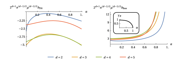
Figure 1: The appropriately rescaled coefficients $b_{\mathrm{Dir}}$ (left image) and $b_{\mathrm{free}}$ (right image) as functions of the parameter $\alpha$ for dimensions two to five. The inset in the right image shows the graph of $\gamma_{R}$ as a function of $\alpha$. We note that $\lim_{\alpha\to 0^{+}}\gamma_{R}\approx 0.9553$ and $\lim_{\alpha\to 1^{-}}\gamma_{R}=0$.

As it turns out, in odd dimensions the integrals in formulae (1.27) and (1.28) can be evaluated explicitly.

Theorem 1.10.

In dimension $d=2k+1$, $k=1,2,\ldots$, formulae (1.27) and (1.28) can be rewritten as

$$b_{\mathrm{Dir}}=-\frac{\mu^{k}}{2^{2k+2}k!\pi^{k}}\left(\left.\frac{2}{k!}\frac{\mathrm{d}^{k}}{\mathrm{d}t^{k}}\left(\frac{2t-\frac{\alpha+1}{\alpha}}{t-\frac{\alpha+1}{\alpha}}\frac{1}{\sqrt{(1-\alpha t)(1-t)}}\right)\right|_{t=0}-2\left(\frac{\alpha}{\alpha+1}\right)^{k}+\alpha^{k}+2k\right),$$ (1.29)

and

$$b_{\mathrm{free}}=\frac{\mu^{k}}{2^{2k+2}k!\pi^{k}}\left(-\frac{8}{k!}\left.\frac{\mathrm{d}^{k}}{\mathrm{d}t^{k}}\left(\frac{\left(2\alpha t^{2}+(\alpha-3)t+2(1-\alpha)\right)\left(4\sqrt{(1-\alpha t)\left(1-t\right)}+(t-2)^{2}\right)}{(t-2)\left(t^{3}-8t^{2}+8(3-2\alpha)t+16(\alpha-1)\right)\sqrt{(1-\alpha t)\left(1-t\right)}}\right)\right|_{t=0}\right.\\ \left.\vphantom{-\frac{8}{k!}\left.\frac{\mathrm{d}^{k}}{\mathrm{d}t^{k}}\left(\frac{\left(2\alpha t^{2}+(\alpha-3)t+2(1-\alpha)\right)\left(4\sqrt{(1-\alpha t)\left(1-t\right)}+(t-2)^{2}\right)}{(t-2)\left(t^{3}-8t^{2}+8(3-2\alpha)t+16(\alpha-1)\right)\sqrt{(1-\alpha t)\left(1-t\right)}}\right)\right|_{t=0}}-\alpha^{k}+2\left(k+2^{2-k}-1\right)\right).$$ (1.30)

The proof of Theorem 1.10 is given in Appendix D.

We list, in Tables 1 and 2, the explicit expressions for $b_{\aleph}$, $\aleph\in\{\mathrm{Dir},\mathrm{free}\}$, for the first few odd dimensions.

$d$	$b_{\mathrm{Dir}}$
$3$	$-\frac{\left(2\alpha^{2}+\alpha+3\right)\mu}{16\pi(\alpha+1)}$
$5$	$-\frac{\left(7\alpha^{4}+12\alpha^{3}+6\alpha^{2}+36\alpha+19\right)\mu^{2}}{512\pi^{2}(\alpha+1)^{2}}$
$7$	$-\frac{\left(13\alpha^{6}+36\alpha^{5}+27\alpha^{4}+16\alpha^{3}+147\alpha^{2}+156\alpha+53\right)\mu^{3}}{12288\pi^{3}(\alpha+1)^{3}}$
$9$	$-\frac{\left(99\alpha^{8}+376\alpha^{7}+500\alpha^{6}+200\alpha^{5}+146\alpha^{4}+1992\alpha^{3}+3188\alpha^{2}+2168\alpha+547\right)\mu^{4}}{1572864\pi^{4}(\alpha+1)^{4}}$

Table 1: The coefficient $b_{\mathrm{Dir}}$ for odd dimensions.

$d$	$b_{\mathrm{free}}$
$3$	$\frac{\left(2\alpha^{2}-3\alpha+3\right)\mu}{16\pi(1-\alpha)}$
$5$	$\frac{\left(-7\alpha^{4}+12\alpha^{3}+14\alpha^{2}-36\alpha+21\right)\mu^{2}}{512\pi^{2}(1-\alpha)^{2}}$
$7$	$\frac{\left(13\alpha^{6}-36\alpha^{5}+30\alpha^{4}-56\alpha^{3}+159\alpha^{2}-168\alpha+62\right)\mu^{3}}{12288\pi^{3}(1-\alpha)^{3}}$
$9$	$\frac{\left(-99\alpha^{8}+376\alpha^{7}-516\alpha^{6}+296\alpha^{5}+470\alpha^{4}-2200\alpha^{3}+3468\alpha^{2}-2440\alpha+661\right)\mu^{4}}{1572864\pi^{4}(1-\alpha)^{4}}$

Table 2: The coefficient $b_{\mathrm{free}}$ for odd dimensions.

Remark 1.11.

1. Integrals in formulae (1.27) and (1.28) can be evaluated explicitly in even dimensions as well, but in this case one ends up with complicated expressions involving elliptic integrals. Given that the outcome would not be much simpler or more elegant than the original formulae (1.27) and (1.28), we omit the explicit evaluation of the integrals in even dimensions.

2. In dimensions $d=2$ and $d=3$, formulae for the second Weyl coefficient for the operator of linear elasticity both for Dirichlet and free boundary conditions are given in [SaVa-97, Section 6.3]. The formulae in [SaVa-97] have been obtained by applying the algorithm described below in §2, but the level of detail therein is somewhat insufficient, with only the final expressions being provided, without any intermediate steps. Our results, when specialised to $d=2$ and $d=3$, agree with those of [SaVa-97] and allow one to recover these results whilst providing the detailed derivation missing in [SaVa-97].

∎

Remark 1.12.

Genquian Liu [Liu-21] claims to have obtained formulae for $\widetilde{b}_{\mathrm{Dir}}$ and $\widetilde{b}_{\mathrm{free}}$. However, the strategy adopted in [Liu-21] is fundamentally flawed, because the “method of images” does not work for the operator of linear elasticity. Consequently, the main results from [Liu-21] are wrong.

We postpone a more detailed discussions of [Liu-21], including the limitations of the method of images and a brief historical account of the development of the subject, until Appendix A. Below, we provide a preliminary “experimental” comparison of our results and those in [Liu-21].

Essentially, [Liu-21] aims to deduce the expression for the second asymptotic heat trace expansion coefficient $\widetilde{b}_{\mathrm{Dir}}$ in the Dirichlet case, as well as a corresponding expression in the case of the boundary conditions [Liu-21, formula (1.5)] (called there the “Neumann” conditions) which in our notation read

$$n^{\beta}\nabla_{\beta}u^{\alpha}=0.$$ (1.31)

We observe that the boundary conditions (1.31) are not self-adjoint for (1.10), as easily seen by simple integration by parts. Therefore, it is hard to assign a meaning to Liu’s result in this case [Liu-21, Theorem 1.1, the lower sign version of formula (1.10)]. Nevertheless, even if one interprets the “Neumann” conditions (1.31) as our free boundary conditions (1.6), as the author suggests in a post-publication revision [Liu-22, formula (1.3)], the result of [Liu-21] in the free boundary case remains wrong.

For the sake of clarity, let us compare the results in the case of Dirichlet boundary conditions only. The main result of [Liu-21] in the Dirichlet case is [Liu-21, Theorem 1.1, the upper sign version of formula (1.10)], which correctly states the coefficient $\widetilde{a}$ (cf. our formulae (1.15) and (1.17)), and also states, in our notation, that

$$\widetilde{b}^{\mathrm{Liu}}_{\mathrm{Dir}}:=-\frac{1}{4(4\pi)^{(d-1)/2}}\left(\frac{d-1}{\mu^{(d-1)/2}}+\frac{1}{(\lambda+2\mu)^{(d-1)/2}}\right).$$ (1.32)

This also implies, by (1.21),

$$b^{\mathrm{Liu}}_{\mathrm{Dir}}=\frac{\widetilde{b}^{\mathrm{Liu}}_{\mathrm{Dir}}}{\Gamma\left(1+\frac{d-1}{2}\right)}=-\frac{\mu^{\frac{1-d}{2}}}{2^{d+1}\pi^{\frac{d-1}{2}}\Gamma\left(\frac{d+1}{2}\right)}\left(\alpha^{(d-1)/2}+d-1\right),$$ (1.33)

which differs from our expression (1.27) by a missing integral term.

For the reasons explained in Appendix A, formula (1.32) is incorrect. We illustrate this by first showing, in Figure 2, the ratio of the coefficient $b^{\mathrm{Liu}}_{\mathrm{Dir}}$ and our coefficient $b_{\mathrm{Dir}}$.

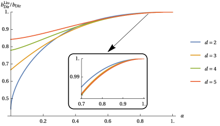
Figure 2: The ratio $b^{\mathrm{Liu}}_{\mathrm{Dir}}/b_{\mathrm{Dir}}$ for different dimensions, shown as functions of $\alpha$.

This ratio depends only on the dimension $d$ and the parameter $\alpha$. For each $d$, the ratio is monotone increasing in $\alpha$ (and is therefore monotone decreasing in $\lambda/\mu$). As $\alpha\to 1^{-}$ (or $\lambda\to-\mu^{+}$), $b^{\mathrm{Liu}}_{\mathrm{Dir}}/b_{\mathrm{Dir}}\to 1^{-}$ in any dimension, see inset to Figure 2. Thus, for the smallest possible values of the Lamé coefficient $\lambda$, Liu’s asymptotic formula would produce an almost correct result, however the error would become more and more noticeable as $\lambda/\mu$ gets large.

We illustrate this phenomenon “experimentally” in Figure 3 where we take $\Omega\subset\mathbb{R}^{2}$ to be the unit square. Neither the Dirichlet nor the free boundary problem in this case can be solved by separation of variables, so we find the eigenvalues using the finite element package FreeFEM [He-12]. As $\operatorname{Vol}_{2}(\Omega)=1$ and $\operatorname{Vol}_{1}(\partial{\Omega})=4$, (1.20) in the Dirichlet case may be interpreted as

$$\mathcal{N}_{\mathrm{Dir}}(\Lambda)-a\Lambda\approx 4b_{\mathrm{Dir}}\sqrt{\Lambda}$$

for sufficiently large $\Lambda$, and we compare the numerically computed left-hand sides with the right-hand sides given by our expression (1.27) and Liu’s expression (1.33). As we have predicted, for $\lambda=-1/2$ both asymptotic formulae give a good agreement with the numerics, however for larger values of $\lambda$ our formulae match the actual eigenvalue counting functions exceptionally well, whereas Liu’s ones are obviously incorrect.

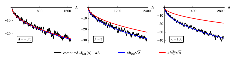
Figure 3: The Dirichlet problem for the unit square. The second Weyl terms, both Liu’s and ours, are compared to the actual numerically computed counting functions. In all three images we take $\mu=1$.

Of course, the boundary of a square is not smooth, only piecewise smooth, but this does not cause problems because this case is covered by [Va-86, Theorem 1]. Furthermore, [Va-86, Theorem 2] guarantees that sufficient conditions ensuring the validity of two-term asymptotic expansions (1.20) are satisfied. ∎

For an additional illustration of the validity of our asymptotics in the free boundary case, see Figure 4. For further examples, both in the Dirichlet and the free boundary case, see Appendices B and C.

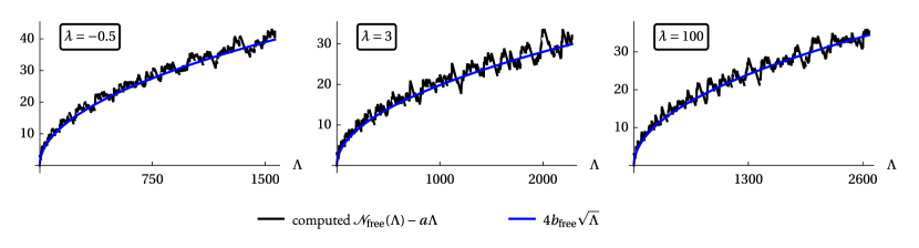
Figure 4: The free boundary problem for the unit square. The second Weyl terms are compared to the actual numerically computed counting functions. In all three images we take $\mu=1$.

Appendix 2.§2.  Second Weyl coefficient for systems: an algorithm

In this section we provide an algorithm for the determination of the second Weyl coefficient for more general elliptic systems. The algorithm given below is not new and appeared in [Va-84, Va-86] as well as in [SaVa-97] for scalar operators, with [Va-84, §6] briefly outlining the changes needed to adapt the results to systems. However, [Va-84, Va-86] are not widely known and their English translations are somewhat unclear; therefore, we reproduce the algorithm here in a self-contained fashion and for matrix operators, for the reader’s convenience. In the next section we will explicitly implement the algorithm for $\mathcal{L}_{\mathrm{Dir}}$ and $\mathcal{L}_{\mathrm{free}}$.

Let $\mathcal{A}$ be a formally self-adjoint elliptic $m\times m$ differential operator of even order $2s$, semibounded from below. Consider the spectral problem

$$\mathcal{A}\mathbf{u}=\Lambda\mathbf{u},$$ (2.1)

$$\left.\mathcal{B}_{j}\mathbf{u}\right|_{\partial\Omega}=0,\qquad j=1,\dots,ms,$$ (2.2)

where the $\mathcal{B}_{j}$’s are differential operators implementing self-adjoint boundary conditions of the Shapiro–Lopatinski type.

It is well-known that the spectrum of (2.1), (2.2) is discrete. Let us denote by

$$\Lambda_{n}^{\mathcal{A},\mathcal{B}},\qquad n\in\mathbb{N},$$

the eigenvalues of (2.1), (2.2), with account of multiplicity, and let

$$\mathcal{N}^{\mathcal{A},\mathcal{B}}(\Lambda):=\#\left\{n:\ \Lambda_{n}^{\mathcal{A},\mathcal{B}}<\Lambda\right\}$$ (2.3)

be the corresponding eigenvalue counting function.

In a neighbourhood of the boundary $\partial\Omega$ we introduce local coordinates

$$x=(x^{\prime},z),\qquad\partial\Omega=\{z=0\},\quad z=\operatorname{dist}(x,\partial\Omega),$$ (2.4)

so that $z>0$ for $x\in\Omega^{\circ}$, where $\Omega^{\circ}$ is the interior of $\Omega$. We will also adopt the notation

$$\xi=(\xi^{\prime},\zeta).$$ (2.5)

Let $\mathcal{A}_{\mathrm{prin}}(x,\xi)$ be the principal symbol of $\mathcal{A}$ and suppose that $\xi\neq 0$. Let $\widetilde{h}_{1}(x,\xi)$, …, $\widetilde{h}_{\widetilde{m}}(x,\xi)$ be the distinct eigenvalues of $\mathcal{A}_{\mathrm{prin}}(x,\xi)$ enumerated in increasing order. Here $\widetilde{m}=\widetilde{m}(x,\xi)$ is a positive integer smaller than or equal to $m$.

Assumption 2.1.

The eigenvalues $\widetilde{h}_{k}(x,\xi)$, $k=1,\ldots,\widetilde{m}$, have constant multiplicities. In particular, the quantity $\widetilde{m}$ is constant, independent of $(x,\xi)$.

We will see in §3 that the above assumption is satisfied for the operator of linear elasticity $\mathcal{L}$.

Theorem 2.2 ([Va-84, Theorem 6.1]).

Suppose that $(\Omega,g)$ is such that the corresponding billiards is neither dead-end nor absolutely periodic. Then the eigenvalue counting function (2.3) admits a two-term asymptotic expansion

$$\mathcal{N}^{\mathcal{A},\mathcal{B}}(\Lambda)=A\,\Lambda^{\frac{d}{2s}}+B_{\mathcal{B}}\Lambda^{\frac{d-1}{2s}}+o\left(\Lambda^{\frac{d-1}{2s}}\right)\quad\text{as}\quad\Lambda\to+\infty$$

for some real constants $A$ and $B_{\mathcal{B}}$. Furthermore:

1. The first Weyl coefficient $A$ is given by

   $$A=\frac{1}{(2\pi)^{d}}\int_{T^{*}\Omega}n(x,\xi,1)\ \mathrm{d}x\,\mathrm{d}\xi,$$

   where $n(x,\xi,\Lambda)$ is the eigenvalue counting function for the matrix-function $\mathcal{A}_{\mathrm{prin}}(x,\xi)$.

2. The second Weyl coefficient $B_{\mathcal{B}}$ is given by

   $$B_{\mathcal{B}}=\frac{1}{(2\pi)^{d-1}}\int_{T^{*}\partial\Omega}\operatorname{shift}(x^{\prime},\xi^{\prime},1)\,\mathrm{d}x^{\prime}\,\mathrm{d}\xi^{\prime}\,,$$ (2.6)

   where the spectral shift function is defined in accordance with

   $$\operatorname{shift}(x^{\prime},\xi^{\prime},\Lambda):=\frac{\varphi(x^{\prime},\xi^{\prime},\Lambda)}{2\pi}+N(x^{\prime},\xi^{\prime},\Lambda)\,,$$

   and the phase shift $\varphi(x^{\prime},\xi^{\prime},\Lambda)$ and the one-dimensional counting function $N(x^{\prime},\xi^{\prime},\Lambda)$ are determined via the algorithm given below.

Step 1: One-dimensional spectral problem. Construct the ordinary differential operators $\mathcal{A}^{\prime}$ and $\mathcal{B}^{\prime}_{j}$ from the partial differential operators $\mathcal{A}$ and $\mathcal{B}_{j}$ as follows:

1. retain only the terms containing the derivatives of the highest order in $\mathcal{A}$ and $\mathcal{B}_{j}$;

2. replace partial derivatives along the boundary with $\mathrm{i}$ times the corresponding component of momentum:

   $$\partial_{x^{\prime}}\mapsto\mathrm{i}\xi^{\prime}\,;$$

3. evaluate all coefficients at $z=0$.

The operators $\mathcal{A}^{\prime}=\mathcal{A}^{\prime}(x^{\prime},\xi^{\prime})$ and $\mathcal{B}^{\prime}_{j}=\mathcal{B}^{\prime}_{j}(x^{\prime},\xi^{\prime})$ are ordinary differential operators in the variable $z$ with coefficients depending on $x^{\prime}$ and $\xi^{\prime}$.

Consider the one-dimensional spectral problem

$$\mathcal{A}^{\prime}\mathbf{u}(z)=\Lambda\mathbf{u}(z),$$ (2.7)

$$\left.\mathcal{B}^{\prime}_{j}\mathbf{u}(z)\right|_{z=0}=0,\qquad j=1,\ldots,sm.$$ (2.8)

Step 2: Thresholds and continuous spectrum. Suppose that $\xi^{\prime}\neq 0$. Let $h_{k}(\zeta)$, $k=1,\dots,\widetilde{m}$, be the distinct eigenvalues of $(\mathcal{A}^{\prime})_{\mathrm{prin}}(\zeta)$ enumerated in increasing order and let $m_{k}$ be their multiplicities, so that

$$\sum_{k=1}^{\widetilde{m}}m_{k}=m.$$

Clearly, for fixed $(x^{\prime},\xi^{\prime})$ we have

$$h_{k}(\zeta)=\widetilde{h}_{k}((x^{\prime},0),(\xi^{\prime},\zeta)),\qquad k=1,\dots,\widetilde{m}\,.$$

In what follows, up to and including Step 6, we suppress, for the sake of brevity, the dependence on $x^{\prime}$ and $\xi^{\prime}$.

Compute the thresholds of the continuous spectrum, namely, nonnegative real numbers $\Lambda_{*}$ such that the equation

$$h_{k}(\zeta)=\Lambda_{*}$$

in the variable $\zeta$ has a multiple real root for at least one $k\in\{1,\ldots,\widetilde{m}\}$. We enumerate the $\overline{m}$ thresholds in increasing order

$$\Lambda_{*}^{(1)}<\dots<\Lambda_{*}^{(\overline{m})}.$$

The thresholds partition the continuous spectrum $[\Lambda_{*}^{(1)},+\infty)$ of the problem (2.7), (2.8) into $\overline{m}$ intervals

$$I^{(l)}:=\begin{cases}\left(\Lambda_{*}^{(l)},\Lambda_{*}^{(l+1)}\right)&\text{for}\ l=1,\ldots,\overline{m}-1,\\[4.30554pt] \left(\Lambda_{*}^{(\overline{m})},+\infty\right)&\text{for}\ l=\overline{m}.\end{cases}$$

For $\Lambda\in I^{(l)}$, let $k_{\mathrm{max}}^{(l)}$ be the largest $k$ for which the equation

$$h_{k}(\zeta)=\Lambda$$ (2.9)

has real roots. Given a $k\in\{1,\ldots,k_{\mathrm{max}}^{(l)}\}$, let $2q_{k}^{(l)}$ be the number of real roots of equation (2.9). We define the multiplicity of the continuous spectrum in $I^{(l)}$ as

$$p^{(l)}:=\sum_{k=1}^{k_{\mathrm{max}}^{(l)}}m_{k}\,q_{k}^{(l)}\,.$$

Step 3: Eigenfunctions of the continuous spectrum. At this step we suppress, for the sake of brevity, the dependence on $l$ and write $k_{\mathrm{max}}=k_{\mathrm{max}}^{(l)}$, $q_{k}=q_{k}^{(l)}$, $p=p^{(l)}$. In each interval $I^{(l)}$ denote the real roots of (2.9) for a given $\,k=1,\ldots,k_{\mathrm{max}}\,$ by

$$\zeta_{k,q}^{\pm}(\Lambda),\qquad q=1,\ldots,q_{k}\,,$$

where the superscript $\pm$ is chosen in such a way that

$$\operatorname{sign}\left(\left.\frac{\mathrm{d}h_{k}(\zeta)}{\mathrm{d}\zeta}\right|_{\zeta=\zeta^{\pm}_{k,q}(\Lambda)}\right)=\pm 1,$$

and the roots are ordered in accordance with

$$\zeta_{k,1}^{-}(\Lambda)<\zeta_{k,1}^{+}(\Lambda)<\ldots<\zeta_{k,q_{k}}^{-}(\Lambda)<\zeta_{k,q_{k}}^{+}(\Lambda)\,.$$

Let

$$\mathbf{v}^{(j)}_{k}(\zeta),\qquad k=1,\ldots,\widetilde{m},\quad j=1,\ldots m_{k},$$

be orthonormal eigenvectors of $(\mathcal{A}^{\prime})_{\mathrm{prin}}(\zeta)$ corresponding to the eigenvalues $h_{k}(\zeta)$. Of course, these eigenvectors are not uniquely defined: there is a $\mathrm{U}(m_{k})$ gauge freedom in their choice.

For given $k\in\{1,\ldots,k_{\mathrm{max}}^{(l)}\}$, $q\in\{1,\ldots,q_{k}\}$ and $@\in\{+,-\}$,  let

$$\mathbf{w}^{@}_{k,q,j}(\Lambda):=\mathbf{v}^{(j)}_{k}(\zeta^{@}_{k,q}(\Lambda)),$$

where the gauge is chosen so that

$$\sum_{j=1}^{m_{k}}\left\langle\mathbf{w}^{@}_{k,q,j}(\Lambda),\frac{\mathrm{d}\mathbf{w}^{@}_{k,q,j}(\Lambda)}{\mathrm{d}\Lambda}\right\rangle=0.$$

This defines each of the two orthonormal bases $\mathbf{w}^{+}_{k,q,j}(\Lambda)\,$, $\,j=1,\ldots m_{k}\,$, and $\mathbf{w}^{-}_{k,q,j}(\Lambda)\,$, $\,j=1,\ldots m_{k}\,$, uniquely modulo a composition of a rigid ($\Lambda$-independent) $\ \mathrm{U}(m_{k})\$ transformation and a $\Lambda$-dependent $\ \mathrm{SU}(m_{k})\$ transformation.

We seek eigenfunctions of the continuous spectrum (generalised eigenfunctions) for the one-dimensional spectral problem (2.7), (2.8) corresponding to $\Lambda\in I^{(l)}$ in the form

$$\begin{split}\mathbf{u}(z;\Lambda)=\sum_{k=1}^{k_{\mathrm{max}}}\sum_{q=1}^{q_{k}}\sum_{j=1}^{m_{k}}&\ \sum_{@\in\{+,-\}}\ \frac{c_{k,q,j}^{@}}{\sqrt{@2\pi\left.(\mathrm{d}h_{k}/\mathrm{d}\zeta)\right|_{\zeta=\zeta^{@}_{k,q}(\Lambda)}}}\mathbf{w}^{@}_{k,q,j}(\Lambda)\,\mathrm{e}^{\mathrm{i}\zeta^{@}_{k,q}(\Lambda)\,z}\\ &+\sum_{r=1}^{ms-p}c_{r}\,\mathbf{f}_{r}(z;\Lambda),\end{split}$$ (2.10)

where $\mathbf{f}_{1}$, …, $\mathbf{f}_{ms-p}$ are linearly independent solutions of (2.7) tending to $0$ as $z\to+\infty$, and the coefficients $c_{k,q,j}^{@}$ are not all zero.

The coefficients $c_{k,q,j}^{@}$ are called incoming ($@=-$) and outgoing ($@=+$) complex wave amplitudes.

Step 4: The scattering matrix. Requiring that (2.10) satisfies the boundary conditions (2.8) allows one to express the outgoing amplitudes $\mathbf{c}^{+}$ in terms of the incoming amplitudes $\mathbf{c}^{-}$. This defines the scattering matrix $S^{(l)}(\Lambda)$, a $p^{(l)}\times p^{(l)}$ unitary matrix, via

$$\mathbf{c}^{+}=S^{(l)}(\Lambda)\,\mathbf{c}^{-}\,.$$

The order in which coefficients $c_{k,q,j}^{@}$ are arranged into $p^{(l)}$-dimensional columns $\mathbf{c}^{@}$ is unimportant.

Step 5: The phase shift. Compute the phase shift $\varphi(\Lambda)$, defined in accordance with

$$\varphi(\Lambda):=\begin{cases}0&\text{for }\Lambda\leq\Lambda_{*}^{(1)},\\ \arg\left(\det S^{(l)}(\Lambda)\right)+\mathfrak{s}^{(l)}&\text{for }\Lambda\in I^{(l)}.\end{cases}$$ (2.11)

The quantities $\mathfrak{s}^{(l)}$, $l=1,\dots,\overline{m}$, are some real constants whose role is to account for the fact that our construction of orthonormal bases for incoming and outgoing complex wave amplitudes involves a rigid ($\Lambda$-independent) unitary gauge degree of freedom, see Step 3 above. The branch of the multi-valued function $\arg$ appearing in formula (2.11) is assumed to be chosen in such a way that the phase shift $\varphi(\Lambda)$ is continuous in each interval $I^{(l)}$.

For each $l$, suppose that equation (2.9) with $\Lambda=\Lambda_{*}^{(l)}$ has a multiple real root for precisely one $k=k^{(l)}$, and that this multiple real root $\zeta=\zeta_{*}^{(l)}$ is unique and is a double root. Then the constants $\mathfrak{s}^{(l)}$ in (2.11) are determined by requiring that the jumps of the phase shift at the thresholds satisfy

$$\frac{1}{\pi}\,\lim_{\epsilon\to 0^{+}}\left(\varphi(\Lambda_{*}^{(l)}+\epsilon)-\varphi(\Lambda_{*}^{(l)}-\epsilon)\right)=j_{*}^{(l)}-\frac{m_{k^{(l)}}}{2}\,,$$ (2.12)

where $j_{*}^{(l)}$ is the number of linearly independent vectors $\mathbf{v}$ such that

$$\mathbf{u}(z)=\mathbf{v}\,\mathrm{e}^{\mathrm{i}\zeta_{*}^{(l)}z}+\mathbf{f}(z)$$ (2.13)

is a solution of the one-dimensional problem (2.7), (2.8), with $\mathbf{f}(z)=o(1)$ as $z\to+\infty$.

The threshold $\Lambda_{*}^{(l)}$ is called rigid if $j_{*}^{(l)}=0$ and soft if $j_{*}^{(l)}=m_{k^{(l)}}$. For rigid and soft thresholds formula (2.12) simplifies and reads

$$\frac{1}{\pi}\,\lim_{\epsilon\to 0^{+}}\left(\varphi(\Lambda_{*}^{(l)}+\epsilon)-\varphi(\Lambda_{*}^{(l)}-\epsilon)\right)=\mp\frac{m_{k^{(l)}}}{2}\,,$$

minus for rigid and plus for soft.

Step 6: The one-dimensional counting function. Compute the one-dimensional counting function

$$N(\Lambda):=\#\{\text{eigenvalues of \eqref{eq:1dimProblA}, \eqref{eq:1dimProblBC} smaller than }\Lambda\}.$$

Application of Steps 1–6 of the above algorithm to the elasticity operator with Dirichlet or free boundary conditions, which will be done in the next three sections, gives

Theorem 2.3.

$$\mathrm{shift}_{\mathrm{Dir}}(\xi^{\prime},\Lambda)=\begin{cases}0&\text{for}\ \Lambda\leq\mu\|\xi^{\prime}\|^{2},\\ -\frac{1}{\pi}\arctan\left(\sqrt{\left(1-\frac{\Lambda}{\lambda+2\mu}\frac{1}{\|\xi^{\prime}\|^{2}}\right)\left(\frac{\Lambda}{\mu}\frac{1}{\|\xi^{\prime}\|^{2}}-1\right)}\right)-\frac{d-1}{4}&\text{for}\ \mu\|\xi^{\prime}\|^{2}<\Lambda<(\lambda+2\mu)\|\xi^{\prime}\|^{2},\\ -\frac{d}{4}&\text{for}\ \Lambda>(\lambda+2\mu)\|\xi^{\prime}\|^{2},\end{cases}$$ (2.14)

and

Theorem 2.4.

$$\mathrm{shift}_{\mathrm{free}}(\xi^{\prime},\Lambda)=\begin{cases}0&\text{for}\ \Lambda<\mu\gamma_{R}^{2}\|\xi^{\prime}\|^{2},\\ 1&\text{for}\ \mu\gamma_{R}^{2}\|\xi^{\prime}\|^{2}<\Lambda<\mu\|\xi^{\prime}\|^{2},\\ \frac{1}{\pi}\arctan\left(\frac{\left(\frac{\Lambda}{\mu}\frac{1}{\|\xi^{\prime}\|^{2}}-2\right)^{2}}{4\,\sqrt{\left(1-\frac{\Lambda}{\lambda+2\mu}\frac{1}{\|\xi^{\prime}\|^{2}}\right)\left(\frac{\Lambda}{\mu}\frac{1}{\|\xi^{\prime}\|^{2}}-1\right)}}\right)+\frac{d-1}{4}&\text{for}\ \mu\|\xi^{\prime}\|^{2}<\Lambda<(\lambda+2\mu)\|\xi^{\prime}\|^{2},\\ \frac{d}{4}&\text{for}\ \Lambda>(\lambda+2\mu)\|\xi^{\prime}\|^{2}.\end{cases}$$ (2.15)

In particular, Theorem 2.3 will follow from (5.1), Lemma 4.1 and Lemma 5.2, whereas Theorem 2.4 will follow from (5.1), Lemma 4.4 and Lemma 5.5.

Substituting (2.14) and (2.15) into (2.6) and performing straightforward algebraic manipulations we arrive at (1.27) and (1.28), respectively, thus proving Theorem 1.8. Note that

$$B_{\aleph}=\mathrm{Vol}_{d-1}(\partial\Omega)\,b_{\aleph},\qquad\aleph\in\{\mathrm{Dir},\mathrm{free}\}\,.$$

Appendix 3.§3.  Second Weyl coefficients for linear elasticity: invariant subspaces

In this and the next two sections we will compute the spectral shift function for the operator of linear elasticity on a Riemannian manifold with boundary of arbitrary dimension $d\geq 2$, both for Dirichlet and free boundary conditions, by explicitly implementing the algorithm from §2. This will establish Theorems 2.3 and 2.4.

In order to substantially simplify the calculations, we will turn some ideas of Dupuis–Mazo–Onsager [DuMaOn-60] into a rigorous mathematical argument, in the spirit of [CaVa-22b]. Namely, we will introduce two invariant subspaces for the elasticity operator compatible with the boundary conditions, implement the algorithm in each invariant subspace separately, and combine the results in the end.

As explained in §1 (see Fact 1.6) it is sufficient to determine the second Weyl coefficients in the Euclidean setting, $g_{\alpha\beta}=\delta_{\alpha\beta}$. Furthermore, the construction presented in the beginning of §2 (see formulae (2.4), (2.5)) allows us to work in a Euclidean half-space. Hence, further on $x=(x^{1},\ldots,x^{d})$ are Cartesian coordinates, $x^{\prime}=(x^{1},\ldots,x^{d-1})$, $z=x^{d}$ and $\Omega=\{z\geq 0\}$. Accordingly, we write $\xi=(\xi_{1},\ldots,\xi_{d})$, $\xi^{\prime}=(\xi_{1},\ldots,\xi_{d-1})$ and $\zeta=\xi_{d}$.

For starters, let us observe that the standard separation of variables leading to the one-dimensional problem (2.7), (2.8) can be achieved by seeking a solution of the form

$$\mathrm{e}^{\mathrm{i}\langle x^{\prime},\xi^{\prime}\rangle}\mathbf{u}(z)\,.$$

Next, suppose we have fixed $\xi^{\prime}\in\mathbb{R}^{d-1}\setminus\{0\}$. Consider the pair of constant $d$-dimensional columns

$$\frac{1}{\|\xi^{\prime}\|}\begin{pmatrix}\xi^{\prime}\\ 0\end{pmatrix},\quad\begin{pmatrix}0^{\prime}\\ 1\end{pmatrix}\,,$$

where $0^{\prime}$ stands for the $(d-1)$-dimensional column of zeros. These define a two-dimensional plane

$$P:=\operatorname{span}\left\{\frac{1}{\|\xi^{\prime}\|}\begin{pmatrix}\xi^{\prime}\\ 0\end{pmatrix}\,,\ \begin{pmatrix}0^{\prime}\\ 1\end{pmatrix}\right\}\subset\mathbb{R}^{d}.$$

Let us denote by $\Pi$ the orthogonal projection onto $P$.

Now, the principal symbol of the elasticity operator reads

$$\mathcal{L}_{\mathrm{prin}}(\xi)=(\mathcal{L}^{\prime})_{\mathrm{prin}}(\zeta)=\mu\|\xi\|^{2}I+(\lambda+\mu)\xi\xi^{T}.$$ (3.1)

Formula (3.1) immediately implies that the eigenvalues of the principal symbol are

$$\widetilde{h}_{1}(\xi)=h_{1}(\zeta)=\mu\|\xi\|^{2},\qquad\text{of multiplicity $m_{1}=d-1$},$$ (3.2)

and

$$\widetilde{h}_{2}(\xi)=h_{2}(\zeta)=(\lambda+2\mu)\|\xi\|^{2},\qquad\text{of multiplicity $m_{2}=1$}.$$ (3.3)

Formulae (1.2), (3.2) and (3.3) imply that Assumption 2.1 is satisfied. The eigenspaces corresponding to (3.2) and (3.3) are

$$(I-\|\xi\|^{-2}\xi\xi^{T})\,\mathbb{R}^{d}\qquad\text{and}\qquad\operatorname{span}\{\xi\},$$

respectively.

It is easy to see that $\xi\in P\,$, $\,P^{\perp}\subset(I-\|\xi\|^{-2}\xi\xi^{T})\,\mathbb{R}^{d}$, and that $P$ and $P^{\perp}$ are invariant subspaces of $\mathcal{L}_{\mathrm{prin}}$. Furthermore, $\left.\mathcal{L}_{\mathrm{prin}}\right|_{P}$ has two simple eigenvalues, $(\lambda+2\mu)\|\xi\|^{2}$ and $\mu\|\xi\|^{2}$, whereas $\left.\mathcal{L}_{\mathrm{prin}}\right|_{P^{\perp}}$ has one eigenvalue $\mu\|\xi\|^{2}$ of multiplicity $d-2$.

The above decomposition can be lifted to the space of vector fields. We define

$$V_{\parallel}:=\{\mathbf{u}\in C^{\infty}[0,+\infty):\mathbf{u}=\Pi\,\mathbf{u}\}$$

and

$$V_{\perp}:=\{\mathbf{u}\in C^{\infty}[0,+\infty):\mathbf{u}=(I-\Pi)\,\mathbf{u}\}\,.$$

Let

$$\mathcal{L}^{\prime}=\mu\left(\|\xi^{\prime}\|^{2}-\frac{\mathrm{d}^{2}}{\mathrm{d}z^{2}}\right)I-(\lambda+\mu)\begin{pmatrix}\mathrm{i}\xi^{\prime}\\ \frac{\mathrm{d}}{\mathrm{d}z}\end{pmatrix}\begin{pmatrix}\mathrm{i}\xi^{\prime}&\frac{\mathrm{d}}{\mathrm{d}z}\end{pmatrix}$$ (3.4)

and

$$\mathcal{T}^{\prime}=-\lambda\begin{pmatrix}0^{\prime}\\ 1\end{pmatrix}\begin{pmatrix}\mathrm{i}\xi^{\prime}&\frac{\mathrm{d}}{\mathrm{d}z}\end{pmatrix}-\mu\left(I\frac{\mathrm{d}}{\mathrm{d}z}+\begin{pmatrix}\mathrm{i}\xi^{\prime}\\ \frac{\mathrm{d}}{\mathrm{d}z}\end{pmatrix}\begin{pmatrix}0^{\prime}&1\end{pmatrix}\right)$$ (3.5)

be the one-dimensional operators associated with $\mathcal{L}$ and $\mathcal{T}$, respectively; recall that the latter are defined by formulae (1.1) and (1.7). It turns out that the linear spaces $V_{\parallel}$ and $V_{\perp}$ are invariant subspaces of $\mathcal{L}^{\prime}$ compatible with the boundary conditions.

Lemma 3.1.

We have

1. $$\mathcal{L}^{\prime}V_{\parallel}\subset V_{\parallel}\,,$$ (3.6)

   $$\mathcal{L}^{\prime}V_{\perp}\subset V_{\perp}\,.$$ (3.7)

2. $$\left.\left(\mathcal{T}^{\prime}V_{\parallel}\right)\right|_{z=0}\subset\left.V_{\parallel}\right|_{z=0}\,,$$ (3.8)

   $$\left.\left(\mathcal{T}^{\prime}V_{\perp}\right)\right|_{z=0}\subset\left.V_{\perp}\right|_{z=0}\,.$$ (3.9)

Proof.

(a) A generic element of $V_{\parallel}$ reads

$$\mathbf{u}_{\parallel}(z)=\frac{1}{\|\xi^{\prime}\|}\begin{pmatrix}\xi^{\prime}\\ 0\end{pmatrix}f_{1}(z)+\begin{pmatrix}0^{\prime}\\ 1\end{pmatrix}f_{2}(z)\,,\qquad f_{1},f_{2}\in C^{\infty}[0,+\infty).$$

Acting with (3.4) on $\mathbf{u}_{\parallel}(z)$ we get

$$\begin{split}(\mathcal{L}^{\prime}\mathbf{u}_{\parallel})(z)&=\mu\|\xi^{\prime}\|^{2}\mathbf{u}_{\parallel}(z)-\mu\frac{1}{\|\xi^{\prime}\|}\begin{pmatrix}\xi^{\prime}\\ 0\end{pmatrix}f_{1}^{\prime\prime}(z)-\mu\begin{pmatrix}0^{\prime}\\ 1\end{pmatrix}f_{2}^{\prime\prime}(z)\\ &-\mathrm{i}(\lambda+\mu)\|\xi^{\prime}\|\begin{pmatrix}\mathrm{i}\xi^{\prime}f_{1}(z)\\ f_{1}^{\prime}(z)\end{pmatrix}-(\lambda+\mu)\begin{pmatrix}\mathrm{i}\xi^{\prime}f_{2}^{\prime}(z)\\ f_{2}^{\prime\prime}(z)\end{pmatrix}\\ &=\frac{1}{\|\xi^{\prime}\|}\begin{pmatrix}\xi^{\prime}\\ 0\end{pmatrix}\left((\lambda+2\mu)\|\xi^{\prime}\|^{2}f_{1}(z)-\mu f_{1}^{\prime\prime}(z)-\mathrm{i}(\lambda+\mu)\|\xi^{\prime}\|f_{2}^{\prime}(z)\right)\\ &+\begin{pmatrix}0^{\prime}\\ 1\end{pmatrix}\left(\mu\|\xi^{\prime}\|^{2}f_{2}(z)-(\lambda+2\mu)f_{2}^{\prime\prime}(z)-\mathrm{i}(\lambda+\mu)\|\xi^{\prime}\|f_{1}^{\prime}(z)\right)\,,\end{split}$$

which is an element of $V_{\parallel}$. This proves (3.6).

A generic element of $V_{\perp}$ reads

$$\mathbf{u}_{\perp}(z)=\sum_{j=1}^{d-2}\begin{pmatrix}\psi_{j}\\ 0\end{pmatrix}f_{j}(z),\qquad f_{j}\in C^{\infty}[0,+\infty),$$

where $\psi_{j}$, $j=1,\dots,d-2$, are linearly independent columns in $\mathbb{R}^{d-1}$ orthogonal to $\xi^{\prime}$. Acting with (3.4) on $\mathbf{u}_{\perp}(z)$ we get

$$(\mathcal{L}^{\prime}\mathbf{u}_{\perp})(z)=\sum_{j=1}^{d-2}\begin{pmatrix}\psi_{j}\\ 0\end{pmatrix}\,\mu\left(\|\xi^{\prime}\|^{2}f_{j}(z)-f_{j}^{\prime\prime}(z)\right)\,,$$

which is an element of $V_{\perp}$. This proves (3.7).

(b) Acting with (3.5) on $\mathbf{u}_{\parallel}(z)$ we get

$$-\left.\left(\mathcal{T}^{\prime}\mathbf{u}_{\parallel}\right)\right|_{z=0}=\frac{1}{\|\xi^{\prime}\|}\begin{pmatrix}\xi^{\prime}\\ 0\end{pmatrix}\left(\mu f_{1}^{\prime}(0)+\mathrm{i}\mu\|\xi^{\prime}\|f_{2}(0)\right)+\begin{pmatrix}0^{\prime}\\ 1\end{pmatrix}\left(\mathrm{i}\lambda\|\xi^{\prime}\|f_{1}(0)+(\lambda+2\mu)f_{2}^{\prime}(0)\right)\,,$$

from which one obtains (3.8).

Acting with (3.5) on $\mathbf{u}_{\perp}(z)$ we get

$$-\left.\left(\mathcal{T}^{\prime}\mathbf{u}_{\perp}\right)\right|_{z=0}=\sum_{j=1}^{d-2}\begin{pmatrix}\psi_{j}\\ 0\end{pmatrix}\,\mu f_{j}^{\prime}(0)\,,$$

which immediately implies (3.9). ∎

Lemma 3.1 implies, via a standard density argument, that the operators $\mathcal{L}^{\prime}_{\aleph}$, $\aleph\in\{\mathrm{Dir},\mathrm{free}\}$, decompose as

$$\mathcal{L}^{\prime}_{\aleph}=\mathcal{L}^{\prime}_{\aleph,\perp}\oplus\mathcal{L}^{\prime}_{\aleph,\parallel},$$

where $\mathcal{L}^{\prime}_{\aleph,\perp}:=\left.\mathcal{L}^{\prime}_{\aleph}\right|_{(I-\Pi)D(\mathcal{L}^{\prime}_{\aleph})}$ and $\mathcal{L}^{\prime}_{\aleph,\parallel}:=\left.\mathcal{L}^{\prime}_{\aleph}\right|_{\Pi D(\mathcal{L}^{\prime}_{\aleph})}$, $D(\mathcal{L}^{\prime}_{\aleph})$ being the domain of $\mathcal{L}^{\prime}_{\aleph}$.

It is then a straightforward consequence of the Spectral Theorem that we can compute the spectral shift function for $\mathcal{L}^{\prime}_{\aleph,\perp}$ and $\mathcal{L}^{\prime}_{\aleph,\parallel}$ separately, and sum up the results in the end. More formally, we have

$$\mathrm{shift}_{\aleph}=\mathrm{shift}_{\aleph,\perp}+\mathrm{shift}_{\aleph,\parallel},\qquad\aleph\in\{\mathrm{Dir},\mathrm{free}\}.$$

Additional simplification: it suffices to implement our algorithm for the special case

$$\xi^{\prime}=\begin{pmatrix}0\\ \vdots\\ 0\\ 1\end{pmatrix}\in\mathbb{R}^{d-1}.$$ (3.10)

The general case can then be recovered by rescaling the spectral parameter in the end, in accordance with

$$\Lambda\mapsto\frac{\Lambda}{\|\xi^{\prime}\|^{2}}\,.$$

In the next two sections, we assume (3.10).

Appendix 4.§4.  First invariant subspace: normally polarised waves

In this section we will compute the spectral shift functions $\mathrm{shift}_{\aleph,\perp}$ for the operators $\mathcal{L}^{\prime}_{\aleph,\perp}$, $\aleph\in\{\mathrm{Dir},\mathrm{free}\}$.

§4.1.  Dirichlet boundary conditions

Consider the spectral problem

$$\mathcal{L}^{\prime}_{\perp}\mathbf{u}_{\perp}=\mu\left(1-\frac{\mathrm{d}^{2}}{\mathrm{d}z^{2}}\right)\mathbf{u}_{\perp}=\Lambda\mathbf{u}_{\perp},$$ (4.1)

$$\mathbf{u}_{\perp}|_{z=0}=0\,.$$ (4.2)

The goal of this subsection is to prove the following result.

Lemma 4.1.

We have

$$\varphi_{\mathrm{Dir},\perp}(\Lambda)=-\frac{(d-2)\pi}{2}\,\chi_{[\mu,+\infty)}(\Lambda)$$

and

$$N_{\mathrm{Dir},\perp}(\Lambda)=0,$$

so that

$$\mathrm{shift}_{\mathrm{Dir},\perp}(\Lambda)=-\frac{d-2}{4}\,\chi_{[\mu,+\infty)}(\Lambda).$$

Here and further on $\chi_{A}$ denotes the indicator function of a set $A\subset\mathbb{R}$.

We shall prove Lemma 4.1 in several steps.

The principal symbol $(\mathcal{L}^{\prime}_{\perp})_{\mathrm{prin}}\,$, as a linear operator in $P^{\perp}$, has only one eigenvalue

$$h_{1,\perp}(\zeta)=h_{1}(\zeta)=\mu(1+\zeta^{2})$$ (4.3)

of multiplicity $m_{1}^{\perp}=d-2$. The eigenvalue (4.3) determines the threshold

$$\Lambda_{*}^{(1)}=\mu$$ (4.4)

which, in turn, yields exponents

$$\zeta_{1,1}^{\pm}(\Lambda)=\pm\sqrt{\frac{\Lambda}{\mu}-1}\,.$$

Therefore, the continuous spectrum of the operator $\mathcal{L}^{\prime}_{\perp}$ contains a single interval $I^{(1)}_{\perp}:=(\mu,+\infty)$ and the multiplicity of the continuous spectrum on this interval is $p_{\perp}^{(1)}=1$. For $\Lambda\in I^{(1)}_{\perp}$, the eigenfunctions of the continuous spectrum read

$$\mathbf{u}_{\perp}(z;\Lambda)=\sum_{j=1}^{d-2}\mathbf{e}_{j}\left(c_{j}^{+}\mathrm{e}^{\mathrm{i}\sqrt{\frac{\Lambda}{\mu}-1}\,z}+c_{j}^{-}\mathrm{e}^{-\mathrm{i}\sqrt{\frac{\Lambda}{\mu}-1}\,z}\right),$$ (4.5)

where $(\mathbf{e}_{j})_{\alpha}=\delta_{j\alpha}$.

Substituting (4.5) into (4.2) we obtain

$$S_{\mathrm{Dir},\perp}^{(1)}(\Lambda)=-\mathrm{I}$$

which, in turn, yields

$$\arg\det S_{\mathrm{Dir},\perp}^{(1)}(\Lambda)=\begin{cases}0\quad\text{if $\,d\,$ is even,}\\ \pi\quad\text{if $\,d\,$ is odd.}\end{cases}$$ (4.6)

Lemma 4.2.

The threshold (4.4) for the problem (4.1), (4.2) is rigid.

Proof.

It is straightforward to see that the problem (4.1), (4.2) does not admit any solution of the form

$$\begin{pmatrix}c_{1}\\ \vdots\\ c_{d-2}\\ 0\\ 0\end{pmatrix},$$ (4.7)

$c_{1},\dots,c_{d-2}\in\mathbb{C}\,$, other than the trivial one, from which the claim follows. ∎

Lemma 4.3.

The problem (4.1), (4.2) does not have eigenvalues.

Proof.

It is easy to see that the problem (4.1), (4.2) does not admit eigenvalues for $\Lambda\geq\mu$, i.e. eigenvalues embedded in the continuous spectrum. Furthermore, for $\Lambda<\mu$ a straightforward substitution shows that the only solution of (4.1), (4.2) of the form

$$\mathbf{u}_{\perp}(z;\Lambda)=\sum_{j=1}^{d-2}\mathbf{e}_{j}c_{j}\mathrm{e}^{-\sqrt{1-\frac{\Lambda}{\mu}}\,z}$$ (4.8)

is the trivial one. This concludes the proof. ∎

Combining formula (4.6), Lemma 4.2 and Lemma 4.3 one obtains Lemma 4.1.

§4.2.  Free boundary conditions

Consider the spectral problem

$$\mathcal{L}^{\prime}_{\perp}\mathbf{u}_{\perp}=\mu\left(1-\frac{\mathrm{d}^{2}}{\mathrm{d}z^{2}}\right)\mathbf{u}_{\perp}=\Lambda\mathbf{u}_{\perp},$$ (4.9)

$$\mathcal{T}^{\prime}\mathbf{u}_{\perp}|_{z=0}=-\mu\,\mathbf{u}_{\perp}^{\prime}(0)=0\,.$$ (4.10)

The goal of this subsection is to prove the following result.

Lemma 4.4.

We have

$$\varphi_{\mathrm{free},\perp}(\Lambda)=\frac{(d-2)\pi}{2}\,\chi_{[\mu,+\infty)}(\Lambda)$$

and

$$N_{\mathrm{free},\perp}(\Lambda)=0,$$

so that

$$\mathrm{shift}_{\mathrm{free},\perp}(\Lambda)=\frac{d-2}{4}\,\chi_{[\mu,+\infty)}(\Lambda).$$

Formulae (4.3)–(4.5) apply unchanged to the free boundary case. Substituting (4.5) into (4.10) we obtain

$$S_{\mathrm{free},\perp}^{(1)}(\Lambda)=\mathrm{I}$$

which, in turn, yields

$$\arg\det S_{\mathrm{free},\perp}^{(1)}(\Lambda)=0.$$ (4.11)

Lemma 4.5.

The threshold (4.4) for the problem (4.9), (4.10) is soft.

Proof.

Result follows from the fact that (4.7) is a solution of (4.9), (4.10) for all $c_{1},\dots,c_{d-2}\in\mathbb{C}\,$. ∎

Lemma 4.6.

The problem (4.9), (4.10) does not have eigenvalues.

Proof.

It is easy to see that the problem (4.9), (4.10) does not admit eigenvalues for $\Lambda\geq\mu$, i.e. eigenvalues embedded in the continuous spectrum. Furthermore, for $\Lambda<\mu$ a straightforward substitution shows that the only solution of (4.9), (4.10) of the form (4.8) is the trivial one. This concludes the proof. ∎

Combining (4.11), Lemma 4.5, and Lemma 4.6, one obtains Lemma 4.4.

Appendix 5.§5.  Second invariant subspace: reduction to the two-dimensional case

In this section we will compute the spectral shift functions $\mathrm{shift}_{\aleph,\parallel}$, $\aleph\in\{\mathrm{Dir},\mathrm{free}\}$, for the $\mathcal{L}^{\prime}_{\parallel}$.

Calculations in the second invariant subspace are trickier, in that, unlike $\mathcal{L}^{\prime}_{\perp}$, the operator $\mathcal{L}^{\prime}_{\parallel}$ is not diagonal. However, our decomposition into invariant subspaces implies the following

Fact 5.1.

Let us denote by $\mathcal{L}_{\mathrm{plane}}$ the operator of linear elasticity for $d=2$. Then the spectral shift function for the problem

$$\mathcal{L}^{\prime}_{\parallel}\mathbf{u}_{\parallel}=\Lambda\mathbf{u}_{\parallel},$$

with Dirichlet/free boundary conditions coincides with the spectral shift function for the operator $\mathcal{L}^{\prime}_{\mathrm{plane}}$ with the same boundary conditions. Namely,

$$\mathrm{shift}_{\aleph,\parallel}(\Lambda)=\mathrm{shift}_{\aleph,\mathrm{plane}}(\Lambda),\qquad\aleph\in\{\mathrm{Dir},\mathrm{free}\}.$$ (5.1)

Fact (5.1) can be easily established by observing that, under assumption (3.10), elements in the domain of $\mathcal{L}^{\prime}_{\parallel}$ are of the form

$$\mathbf{u}_{\parallel}(z)=\begin{pmatrix}0\\ \vdots\\ 0\\ f_{1}(z)\\ f_{2}(z)\end{pmatrix}\,.$$

In the remainder of this section we will compute the spectral shift function for the operator of linear elasticity in dimension two.

The principal symbol $\left(\mathcal{L}^{\prime}_{\mathrm{plane}}\right)_{\mathrm{prin}}$ has two simple eigenvalues

$$h_{1}(\zeta)=\mu(1+\zeta^{2}),\qquad h_{2}(\zeta)=(\lambda+2\mu)(1+\zeta^{2})\,.$$

These give us the two thresholds

$$\Lambda_{*}^{(1)}=\mu,\qquad\Lambda_{*}^{(2)}=\lambda+2\mu$$

and the corresponding exponents

$$\zeta_{1}^{\pm}(\Lambda)=\pm\sqrt{\frac{\Lambda}{\mu}-1}\,,\qquad\zeta_{2}^{\pm}(\Lambda)=\pm\sqrt{\frac{\Lambda}{\lambda+2\mu}-1}\,,$$

so that the continuous spectrum $[\mu,+\infty)$ is partitioned into the two intervals

$$I^{(1)}=(\mu,\lambda+2\mu),\qquad I^{(2)}=(\lambda+2\mu,+\infty)$$

of multiplicities $p^{(1)}=1$ and $p^{(2)}=2$, respectively.

The normalised eigenvectors of $\left(\mathcal{L}^{\prime}_{\mathrm{plane}}\right)_{\mathrm{prin}}$ are

$$\mathbf{v}_{1}(\zeta)=\frac{1}{\sqrt{1+\zeta^{2}}}\begin{pmatrix}1\\ \zeta\end{pmatrix}\,,\qquad\mathbf{v}_{2}(\zeta)=\frac{1}{\sqrt{1+\zeta^{2}}}\begin{pmatrix}-\zeta\\ 1\end{pmatrix}\,.$$

Hence, the eigenfunctions of the continuous spectrum for $\Lambda$ in $I^{(1)}$ and $I^{(2)}$ read

$$\mathbf{u}(z;\Lambda)=\sum_{@\in\{+,-\}}\frac{1}{\sqrt{@4\pi\mu\,\zeta_{1}^{@}(\Lambda)}}c_{1}^{@}\,\mathbf{v}_{1}(\zeta_{1}^{@}(\Lambda))\mathrm{e}^{\mathrm{i}\zeta_{1}^{@}(\Lambda)\,z}+c\,\mathbf{v}_{2}\left(\mathrm{i}\sqrt{1-\frac{\Lambda}{\lambda+2\mu}}\right)\mathrm{e}^{-\sqrt{1-\frac{\Lambda}{\lambda+2\mu}}\,z}$$ (5.2)

and

$$\begin{split}\mathbf{u}(z;\Lambda)=\sum_{@\in\{+,-\}}&\left(\frac{1}{\sqrt{4\pi\mu\,|\zeta_{1}^{@}(\Lambda)}|}c_{1}^{@}\,\mathbf{v}_{1}(\zeta_{1}^{@}(\Lambda))\mathrm{e}^{\mathrm{i}\zeta_{1}^{@}(\Lambda)\,z}\right.\\ &\ +\left.\frac{1}{\sqrt{4\pi(\lambda+2\mu)\,|\zeta_{2}^{@}(\Lambda)}|}c_{2}^{@}\,\mathbf{v}_{2}(\zeta_{2}^{@}(\Lambda))\mathrm{e}^{\mathrm{i}\zeta_{2}^{@}(\Lambda)\,z}\right),\end{split}$$ (5.3)

respectively.

§5.1.  Dirichlet boundary conditions

Consider the spectral problem

$$\mathcal{L}_{\mathrm{plane}}^{\prime}\mathbf{u}=\begin{pmatrix}\lambda+2\mu-\mu\frac{\mathrm{d}^{2}}{\mathrm{d}z^{2}}&-\mathrm{i}(\lambda+\mu)\frac{\mathrm{d}}{\mathrm{d}z}\\ -\mathrm{i}(\lambda+\mu)\frac{\mathrm{d}}{\mathrm{d}z}&\mu-(\lambda+2\mu)\frac{\mathrm{d}^{2}}{\mathrm{d}z^{2}}\\ \end{pmatrix}\begin{pmatrix}f_{1}(z)\\ f_{2}(z)\end{pmatrix}=\Lambda\begin{pmatrix}f_{1}(z)\\ f_{2}(z)\end{pmatrix},$$ (5.4)

$$\begin{pmatrix}f_{1}(0)\\ f_{2}(0)\end{pmatrix}=\begin{pmatrix}0\\ 0\end{pmatrix}\,.$$ (5.5)

The goal of this subsection is to prove the following result.

Lemma 5.2.

We have

$$\varphi_{\mathrm{Dir},\mathrm{plane}}(\Lambda)=\begin{cases}0&\text{for}\ \Lambda<\mu,\\ -2\arctan\left(\sqrt{\left(1-\frac{\Lambda}{\lambda+2\mu}\right)\left(\frac{\Lambda}{\mu}-1\right)}\right)-\frac{\pi}{2}&\text{for}\ \mu<\Lambda<\lambda+2\mu,\\ -\pi&\text{for}\ \Lambda>\lambda+2\mu\end{cases}$$

and

$$N_{\mathrm{Dir},\mathrm{plane}}(\Lambda)=0,$$

so that

$$\mathrm{shift}_{\mathrm{Dir},\mathrm{plane}}(\Lambda)=\begin{cases}0&\text{for}\ \Lambda<\mu,\\ -\frac{1}{\pi}\arctan\left(\sqrt{\left(1-\frac{\Lambda}{\lambda+2\mu}\right)\left(\frac{\Lambda}{\mu}-1\right)}\right)-\frac{1}{4}&\text{for}\ \mu<\Lambda<\lambda+2\mu,\\ -\frac{1}{2}&\text{for}\ \Lambda>\lambda+2\mu.\end{cases}$$

We shall prove Lemma 5.2 in several steps.

Substituting (5.2) and (5.3) into (5.5) we get

$$S_{\mathrm{Dir},\mathrm{plane}}(\Lambda)=\begin{cases}\frac{\sqrt{(1-\frac{\Lambda}{\lambda+2\mu})(\frac{\Lambda}{\mu}-1)}+\mathrm{i}}{\sqrt{(1-\frac{\Lambda}{\lambda+2\mu})(\frac{\Lambda}{\mu}-1)}-\mathrm{i}}&\text{for}\ \Lambda\in I^{(1)},\\[15.00002pt] \begin{pmatrix}\frac{\sigma^{2}-1}{\sigma^{2}+1}&-\frac{2\sigma}{\sigma^{2}+1}\\ \frac{2\sigma}{\sigma^{2}+1}&\frac{\sigma^{2}-1}{\sigma^{2}+1}\end{pmatrix}&\text{for}\ \Lambda\in I^{(2)},\end{cases}$$

where $\sigma:=\left(\frac{\Lambda}{\mu}-1\right)^{1/4}\left(\frac{\Lambda}{\lambda+2\mu}-1\right)^{1/4}$. The above equation implies

$$\arg\det S_{\mathrm{Dir},\mathrm{plane}}(\Lambda)=\begin{cases}-2\arctan\left(\sqrt{\left(1-\frac{\Lambda}{\lambda+2\mu}\right)\left(\frac{\Lambda}{\mu}-1\right)}\right)&\text{for}\ \Lambda\in I^{(1)},\\ 0&\text{for}\ \Lambda\in I^{(2)}.\end{cases}$$ (5.6)

Lemma 5.3.

The thresholds $\Lambda_{*}^{(1)}$ and $\Lambda_{*}^{(2)}$ for the problem (5.4), (5.5) are rigid.

Proof.

Let us first consider $\Lambda_{*}^{(1)}$. The general solution to (5.4) of the form (2.13) reads

$$c_{1}\begin{pmatrix}1\\ \mathrm{i}\sqrt{\frac{\lambda+\mu}{\lambda+2\mu}}\end{pmatrix}\mathrm{e}^{-\sqrt{\frac{\lambda+\mu}{\lambda+2\mu}}\,z}+c_{2}\begin{pmatrix}0\\ 1\end{pmatrix}.$$ (5.7)

Substituting the above expression into (5.5) gives us $c_{1}=c_{2}=0$. Hence, $\Lambda_{*}^{(1)}$ is rigid.

Let us now examine $\Lambda_{*}^{(2)}$. The general solution to (5.4) of the form (2.13) reads

$$c\begin{pmatrix}1\\ 0\end{pmatrix}.$$ (5.8)

The latter can only satisfy the Dirichlet boundary conditions if $c=0$, which implies that $\Lambda_{*}^{(2)}$ is rigid as well. ∎

Lemma 5.4.

The problem (5.4), (5.5) does not have eigenvalues, either below or embedded in the continuous spectrum.

Proof.

Arguing as in the proof of Lemma 5.3, it is easy to see that thresholds are not eigenvalues.

For $\Lambda\in(0,\mu)$ we seek an eigenfunction of (5.4) in the form

$$\mathbf{u}(z;\Lambda)=c_{1}\,\mathbf{v}_{1}\left(\mathrm{i}\sqrt{1-\frac{\Lambda}{\mu}}\right)\mathrm{e}^{-\sqrt{1-\frac{\Lambda}{\mu}}\,z}+c_{2}\,\mathbf{v}_{2}\left(\mathrm{i}\sqrt{1-\frac{\Lambda}{\lambda+2\mu}}\right)\mathrm{e}^{-\sqrt{1-\frac{\Lambda}{\lambda+2\mu}}\,z}\,.$$ (5.9)

Substituting (5.9) into (5.5) we get

$$\begin{pmatrix}1&-\mathrm{i}\sqrt{1-\frac{\Lambda}{\lambda+2\mu}}\\ \mathrm{i}\sqrt{1-\frac{\Lambda}{\mu}}&1\end{pmatrix}\begin{pmatrix}c_{1}\\ c_{2}\end{pmatrix}=\begin{pmatrix}0\\ 0\end{pmatrix},$$

so that the characteristic equation in $(0,\mu)$ reads

$$\chi(\Lambda)=1-\sqrt{1-\frac{\Lambda}{\lambda+2\mu}}\sqrt{1-\frac{\Lambda}{\mu}}=0.$$

The latter has no solutions in $(0,\mu)$.

For $\Lambda\in I^{(1)}$ we seek an eigenfunction in the form (5.2) with $c_{1}^{\pm}=0$, so that the solution is square-integrable:

$$\mathbf{u}(z;\Lambda)=c\,\mathbf{v}_{2}\left(\mathrm{i}\sqrt{1-\frac{\Lambda}{\lambda+2\mu}}\right)\mathrm{e}^{-\sqrt{1-\frac{\Lambda}{\lambda+2\mu}}\,z}.$$ (5.10)

The latter satisfies (5.5) if and only if $c=0$, which means there are no eigenfunctions for $\Lambda\in I^{(1)}$,

By looking at (5.3), it is easy to see that there are no (square-integrable) eigenfunctions corresponding to $\Lambda\in I^{(2)}$, which completes the proof. ∎

Combining (5.6), Lemma 5.3, and Lemma 5.4, one obtains Lemma 5.2.

§5.2.  Free boundary conditions

Consider the spectral problem

$$\mathcal{L}_{\mathrm{plane}}^{\prime}\mathbf{u}=\begin{pmatrix}\lambda+2\mu-\mu\frac{\mathrm{d}^{2}}{\mathrm{d}z^{2}}&-\mathrm{i}(\lambda+\mu)\frac{\mathrm{d}}{\mathrm{d}z}\\ -\mathrm{i}(\lambda+\mu)\frac{\mathrm{d}}{\mathrm{d}z}&\mu-(\lambda+2\mu)\frac{\mathrm{d}^{2}}{\mathrm{d}z^{2}}\\ \end{pmatrix}\begin{pmatrix}f_{1}(z)\\ f_{2}(z)\end{pmatrix}=\Lambda\begin{pmatrix}f_{1}(z)\\ f_{2}(z)\end{pmatrix},$$ (5.11)

$$-\left.\left(\mathcal{T}^{\prime}\mathbf{u}\right)\right|_{z=0}=\begin{pmatrix}\mu(f_{1}^{\prime}(0)+\mathrm{i}f_{2}(0))\\ \mathrm{i}\lambda f_{1}(0)+(\lambda+2\mu)f_{2}^{\prime}(0)\end{pmatrix}=\begin{pmatrix}0\\ 0\end{pmatrix}\,.$$ (5.12)

The goal of this subsection is to prove the following result.

Lemma 5.5.

We have

$$\varphi_{\mathrm{free},\mathrm{plane}}(\Lambda)=\begin{cases}0&\text{for}\ \Lambda<\mu,\\ 2\arctan\left(\frac{\left(\frac{\Lambda}{\mu}-2\right)^{2}}{4\,\sqrt{\left(1-\frac{\Lambda}{\lambda+2\mu}\right)\left(\frac{\Lambda}{\mu}-1\right)}}\right)-\frac{3\pi}{2}&\text{for}\ \mu<\Lambda<\lambda+2\mu,\\ -\pi&\text{for}\ \Lambda>\lambda+2\mu\end{cases}$$

and

$$N_{\mathrm{free},\mathrm{plane}}(\Lambda)=\chi_{(\gamma_{R}^{2}\mu,+\infty)}(\Lambda),$$

where $\gamma_{R}$ is given by (1.24), so that

$$\mathrm{shift}_{\mathrm{free},\mathrm{plane}}(\Lambda)=\begin{cases}0&\text{for}\ \Lambda<\mu\gamma_{R}^{2},\\ 1&\text{for}\ \mu\gamma_{R}^{2}<\Lambda<\mu,\\ \frac{1}{\pi}\arctan\left(\frac{\left(\frac{\Lambda}{\mu}-2\right)^{2}}{4\,\sqrt{\left(1-\frac{\Lambda}{\lambda+2\mu}\right)\left(\frac{\Lambda}{\mu}-1\right)}}\right)+\frac{1}{4}&\text{for}\ \mu<\Lambda<\lambda+2\mu,\\ \frac{1}{2}&\text{for}\ \Lambda>\lambda+2\mu.\end{cases}$$

We shall prove Lemma 5.5 in several steps.

Substituting (5.2) and (5.3) into (5.12) we get

$$\arg\det S_{\mathrm{free},\mathrm{plane}}(\Lambda)=\begin{cases}2\arctan\left(\frac{\left(\frac{\Lambda}{\mu}-2\right)^{2}}{4\,\sqrt{\left(1-\frac{\Lambda}{\lambda+2\mu}\right)\left(\frac{\Lambda}{\mu}-1\right)}}\right)&\text{for}\ \Lambda\in I^{(1)},\\ 0&\text{for}\ \Lambda\in I^{(2)}.\end{cases}$$ (5.13)

We now have

Lemma 5.6.

1. The threshold $\Lambda_{*}^{(1)}$ for the problem (5.11), (5.12) is rigid. That is,

   $$j_{*}^{(1)}=0.$$

2. The threshold $\Lambda_{*}^{(2)}$ for the problem (5.11), (5.12) is soft if $\lambda=0$ and rigid otherwise. That is,

   $$j_{*}^{(2)}=\begin{cases}0&\text{for }\lambda\neq 0,\\ 1&\text{for }\lambda=0.\end{cases}$$

Proof.

(a) Substituting (5.7) into (5.12) we obtain the linear system

$$\begin{pmatrix}-2\sqrt{\frac{\lambda+\mu}{\lambda+2\mu}}&\mathrm{i}\\ -\mathrm{i}\mu&0\end{pmatrix}\begin{pmatrix}c_{1}\\ c_{2}\end{pmatrix}=\begin{pmatrix}0\\ 0\end{pmatrix},$$

which has no nontrivial solutions. Indeed,

$$\det\begin{pmatrix}-2\sqrt{\frac{\lambda+\mu}{\lambda+2\mu}}c_{1}&\mathrm{i}\\ -\mathrm{i}\mu&0\end{pmatrix}=-\mu<0\,.$$

(b) The claim follows at once by substituting (5.8) into (5.12). ∎

Lemma 5.7.

The problem (5.11), (5.12) has precisely one eigenvalue

$$\Lambda_{R}:=\mu\gamma_{R}^{2}\,,$$ (5.14)

where $\gamma_{R}$ is given by (1.24).

Proof.

Arguing as in the proof of Lemma 5.6, it is easy to see that thresholds are not eigenvalues.

For $\Lambda\in(0,\mu)$, we seek an eigenfunction in the form (5.9). Substituting (5.9) into (5.12) we get

$$\begin{pmatrix}-2\sqrt{1-\frac{\Lambda}{\lambda+2\mu}}&\mathrm{i}\left(2-\frac{\Lambda}{\mu}\right)\\ -\mathrm{i}\mu\left(2-\frac{\Lambda}{\mu}\right)&-2\mu\sqrt{1-\frac{\Lambda}{\mu}}\end{pmatrix}\begin{pmatrix}c_{1}\\ c_{2}\end{pmatrix}=\begin{pmatrix}0\\ 0\end{pmatrix}.$$

Therefore, the characteristic equation reads

$$\chi(\Lambda)=4\sqrt{1-\frac{\Lambda}{\lambda+2\mu}}\sqrt{1-\frac{\Lambda}{\mu}}-\left(2-\frac{\Lambda}{\mu}\right)^{2}=0\,,\qquad\Lambda\in(0,\mu).$$

We observe that

$$\chi(\mu\Lambda)=\widetilde{R}_{\alpha}(\Lambda),$$ (5.15)

cf. (1.26). But $\widetilde{R}_{\alpha}(\Lambda)=0$ has a unique solution $\Lambda=\gamma_{R}^{2}$ in $(0,1)$, as discussed in Remark 1.7. Hence, (5.15) implies (5.14).

For $\Lambda\in I^{(1)}$ we seek an eigenfunction in the form (5.10). Substituting (5.10) into (5.12), one sees that the latter can only be satisfied if $c=0$. Therefore, there are no eigenvalues in $I^{(1)}$.

Lastly, by looking at (5.3), it is easy to see that there are no (square-integrable) eigenfunctions corresponding to $\Lambda\in I^{(2)}$. This concludes the proof. ∎

Observe that $\Lambda_{R}<\Lambda_{*}^{(1)}$, that is, the Rayleigh eigenvalue is located below the continuous spectrum.

Combining (5.13), Lemma 5.6, and Lemma 5.7, one obtains Lemma 5.5.

Note that in Lemma 5.5 there is no distinction between the cases $\lambda\neq 0$ and $\lambda=0$, which prima facie may seem at odds with Lemma 5.6. However, there is no contradiction, because the different values of $j_{*}^{(2)}$ in the two cases are compensated exactly by the different values of the jump of (5.13) at the threshold $\Lambda_{*}^{(2)}$:

$$\frac{1}{\pi}\,\lim_{\epsilon\to 0^{+}}\left(\arg\det S_{\mathrm{free},\mathrm{plane}}(\Lambda_{*}^{(2)}+\epsilon)-\arg\det S_{\mathrm{free},\mathrm{plane}}(\Lambda_{*}^{(2)}-\epsilon)\right)=\begin{cases}-1&\text{for }\lambda\neq 0,\\ 0&\text{for }\lambda=0.\end{cases}$$

Appendix A On the paper [Liu-21]

In this appendix, we continue the discussion of the paper [Liu-21], which we started in Remark 1.12.

Let us begin by observing that, at a qualitative level, the two-term expansion [Liu-21, Theorem 1.1] cannot be correct, because the two leading coefficients in the heat trace expansion have the same structure in the way the Lamé parameters appear in these coefficients. The boundary conditions mix up longitudinal and transverse waves; hence one expects that contributions from the Lamé parameters $\lambda$ and $\mu$ would mix up in a rather complicated way in the second coefficient. Mathematically, the reason for the erroneous expressions comes from the fact that the method of images does not work for the operator of linear elasticity, as we explain below.

For simplicity, in the spirit of Fact 1.6, we work in Euclidean space $\mathbb{R}^{2}$ endowed with coordinates $(x,y)$, with $\Omega:=\{(x,y)\,|\,y>0\}$ being the upper half-plane and its boundary $\partial\Omega$ being the $x$-axis $\{y=0\}$.

Let $\tau:(x,y)\mapsto(x,-y)$ be a reflection with respect to the $x$-axis. For a function $u$ (vector- or scalar-valued), consider the involution $Ju:=u\circ\tau$, so that $(Ju)(x,y)=u(x,-y)$. It is obvious that $J$ commutes with either the vector or the scalar Laplacian on sufficiently smooth functions:

$$(J\circ\Delta)u=(\Delta\circ J)u=\left.(\Delta u)\right|_{\text{evaluated at the point }(x,-y)}.$$

Let now $\mathcal{L}$ be the elasticity operator, which acts on vector-valued functions $\mathbf{u}(x,y)=\begin{pmatrix}u_{1}(x,y)\\ u_{2}(x,y)\end{pmatrix}$ as

$$\mathcal{L}\mathbf{u}=\begin{pmatrix}-\mu\Delta-(\lambda+\mu)\partial^{2}_{xx}&-(\lambda+\mu)\partial^{2}_{xy}\\ -(\lambda+\mu)\partial^{2}_{xy}&-\mu\Delta-(\lambda+\mu)\partial^{2}_{yy}\end{pmatrix}\begin{pmatrix}u_{1}\\ u_{2}\end{pmatrix}=\begin{pmatrix}-(\lambda+2\mu)\partial^{2}_{xx}u_{1}-\mu\partial^{2}_{yy}u_{1}-(\lambda+\mu)\partial^{2}_{xy}u_{2}\\ -(\lambda+2\mu)\partial^{2}_{yy}u_{2}-\mu\partial^{2}_{xx}u_{2}-(\lambda+\mu)\partial^{2}_{xy}u_{1}\end{pmatrix}.$$

Then

$$(J\circ\mathcal{L})\mathbf{u}=\left.(\mathcal{L}\mathbf{u})\right|_{\text{evaluated at the point }(x,-y)},$$

but by the chain rule

$$(\mathcal{L}\circ J)\mathbf{u}=\left.\begin{pmatrix}-(\lambda+2\mu)\partial^{2}_{xx}u_{1}-\mu\partial^{2}_{yy}u_{1}+(\lambda+\mu)\partial^{2}_{xy}u_{2}\\ -(\lambda+2\mu)\partial^{2}_{yy}u_{2}-\mu\partial^{2}_{xx}u_{2}+(\lambda+\mu)\partial^{2}_{xy}u_{1}\end{pmatrix}\right|_{\text{evaluated at the point }(x,-y)}$$

(i.e., the signs of the off-diagonal terms involving mixed derivatives change), and therefore the commutator $[J,\mathcal{L}]$ does not vanish. Since the elasticity operator does not commute with reflections, the reflection method (or the method of images) is inapplicable.

The above argument shows that the principal symbol of the Laplacian (or the Laplace–Beltrami operator when working in curved space) is invariant under reflection, whereas the principal symbol of the operator of linear elasticity is not. This is what makes the method of images work for the Laplacian, but not for the operator of linear elasticity. The key difference between the Laplacian (or the Laplace–Beltrami operator) and the operator of linear elasticity is the presence of mixed derivatives in the leading term of the latter.

For the reader’s convenience, let us spell out the precise points in [Liu-21] where the main mistakes occur, as a result of the operator $\mathcal{L}$ not being invariant under reflections. Below we use the notation from [Liu-21].

The author defines $\mathcal{M}:=\Omega\cup\partial\Omega\cup\Omega^{*}$ to be the “double” of $\Omega$, and $\mathcal{P}$ to be the “double” of the operator of linear elasticity in $\mathcal{M}$. In the simplified setting of this appendix, $\mathcal{M}=\mathbb{R}^{2}$ and

$$\mathcal{P}:=\begin{cases}\mathcal{L}&\text{in }\Omega=\{y>0\}\,,\\ \mathcal{L}+2(\lambda+\mu)\begin{pmatrix}0&\partial_{x}\\ \partial_{x}&0\end{pmatrix}\frac{\partial}{\partial y}&\text{in }\Omega^{*}=\{y<0\}\,.\end{cases}$$

Given $\mathbf{u},\mathbf{v}\in C^{\infty}_{c}(\mathbb{R}^{2})$ (the space of infinitely smooth functions with compact support), by a straightforward integration by parts one obtains

$$(\mathcal{P}\mathbf{u},\mathbf{v})-(\mathbf{u},\mathcal{P}\mathbf{v})=4(\lambda+\mu)\int_{\{y=0\}}\left(\partial_{x}u_{1}\,\overline{v_{2}}-u_{2}\,\overline{\partial_{x}v_{1}}\right)\,\mathrm{d}x\,.$$ (A.1)

Here $(\cdot\,,\,\cdot)$ denotes the natural $L^{2}$ inner product and overline denotes complex conjugation. But (A.1) implies that $\mathcal{P}$ is not symmetric; therefore, it does not give rise to a heat operator.

As a result, the statement “$\mathcal{P}$ generates a strongly continuous semigroup $\left(e^{t\mathcal{P}}\right)_{t\geq 0}$ on $L^{2}(\mathcal{M})$ with integral kernel $K(t,x,y)$” in [Liu-21, p. 10169, third line after (1.14)] is wrong, and all the analysis based on it breaks down (including [Liu-21, formula (4.3)]).

In [Liu-21], the author states that they borrow their technique from McKean and Singer [McKSi-67]. Indeed, the paragraph preceding formula (4.3) in [Liu-21, p. 10183] is taken, almost verbatim, from the beginning of Section 5 of [McKSi-67, p. 53]. However, McKean and Singer applied the method of images to the Laplacian, for which the “double” operator is self-adjoint.

Let us conclude this appendix with a brief historical account. We note that the expression for $\widetilde{b}_{\mathrm{Dir}}$ was already found in the 1960 paper by M. Dupuis, R. Mazo, and L. Onsager [DuMaOn-60]. Remarkably, this paper includes the critique of the 1950 paper by E. W. Montroll who presented exactly Liu’s expression (1.32) for the second asymptotic coefficient, modulo some scaling, see [Mo-50, formulae (3)–(5)]. Dupuis, Mazo, and Onsager wrote, we quote: “Montroll …pointed out in 1950 a defect in the usual counting process of the normal modes of vibration and derived a corresponding correction term for the Debye frequency spectrum, …, proportional to the area of the solid. But it must be clearly realized that he used as a model a parallelopiped with perfectly reflecting faces, and that such boundary conditions are not realistic. It is well known that in the case of a free surface as well as in the case of a clamped surface, one cannot satisfy the boundary conditions by the simple superposition of an incident wave and of a reflected wave of the same kind; one must add a transverse reflected wave if the incident is longitudinal and vice versa. The surface ”scrambles” the waves so that one can no longer analyze the vibrations of the solid in terms of pure transverse and pure longitudinal modes.”

The results of Dupuis, Mazo, and Onsager for $d=3$ were reproduced, for both the Dirichlet and the free boundary conditions, as rigorous theorems in [SaVa-97, Section 6.3], who also extended these results to the planar case $d=2$.

Appendix B A two-dimensional example: the disk

Our aim in this (and in the next) appendix to give an experimental verification of the correctness of the second asymptotic coefficients (1.27) and (1.28) and to demonstrate the incorrectness of the second asymptotic coefficient (1.32)–(1.33). We work with counting functions rather than with partition functions since the former can, in some cases, be explicitly calculated for reasonably large values of the parameter, whereas computing the latter would require additional trickery.

Let $\Omega\subset\mathbb{R}^{d}$ be the unit disk, equipped with standard polar coordinates $(r,\phi)$. The equations of elasticity (1.10) with Dirichlet boundary conditions in the disk allow the separation of variables. To this end, we, in essence, separate variables in the three-dimensional cylinder $\Omega\times\mathbb{R}$ following [MoFe-53, Chapter XIII] and looking for solutions independent of the third coordinate, cf. also [LeMoSe-21, Supplementary materials]. More precisely, we take

$$u(r,\phi)=\operatorname{grad}\psi_{1}(r,\phi)+\operatorname{curl}\left(\mathbf{z}\,\psi_{2}(r,\phi)\right),$$ (B.1)

where $\mathbf{z}$ is the third coordinate vector. Then it is easily seen that the scalar potentials $\psi_{j}(r,\phi)$, $j=1,2$, should satisfy the Helmholtz equations

$$-\Delta\psi_{j}=\omega_{j,\Lambda}\psi_{j},$$ (B.2)

where

$$\omega_{1,\Lambda}:=\frac{\Lambda}{\lambda+2\mu},\qquad\omega_{2,\Lambda}:=\frac{\Lambda}{\mu}.$$ (B.3)

The general solution of (B.2) regular at the origin is well-known,

$$\psi_{j}(r,\phi)=c_{j,0}J_{0}\left(\sqrt{\omega_{j,\Lambda}}r\right)+\sum_{k=1}^{\infty}J_{k}\left(\sqrt{\omega_{j,\Lambda}}r\right)\left(c_{j,k,+}\mathrm{e}^{\mathrm{i}k\phi}+c_{j,k,-}\mathrm{e}^{-\mathrm{i}k\phi}\right),$$ (B.4)

where the $J_{k}$ are Bessel functions, and the $c$’s are constants. Substituting (B.1), (B.3), and (B.4) into the boundary condition $u(1,\phi)=0$ leads, after simplifications, to the secular equations

$$J_{1}\left(\sqrt{\omega_{1,\Lambda}}\right)J_{1}\left(\sqrt{\omega_{2,\Lambda}}\right)=0,\qquad\text{if }k=0,$$ (B.5)

and

$$\frac{k}{\sqrt{\mu}}J_{k}\left(\sqrt{\omega_{1,\Lambda}}\right)J_{k+1}\left(\sqrt{\omega_{2,\Lambda}}\right)+\frac{J_{k+1}\left(\sqrt{\omega_{2,\Lambda}}\right)}{\sqrt{\lambda+2\mu}}\left(kJ_{k}\left(\sqrt{\omega_{2,\Lambda}}\right)-\omega_{2,\Lambda}J_{k}\left(\sqrt{\omega_{2,\Lambda}}\right)\right)=0,\qquad\text{if }k>0.$$ (B.6)

Every solution $\Lambda>0$ of the secular equation (B.5) is an eigenvalue of multiplicity one of the Dirichlet elasticity operator $\mathcal{L}^{\mathrm{Dir}}$ on the unit disk, and every solution $\Lambda>0$ of the secular equation (B.6) is an eigenvalue of multiplicity two.

Note that for the case of the disk the branching Hamiltonian billiards associated with the operator of elasticity can be analysed explicitly, and one can check that the two-term asymptotics (1.20) is valid.

The numerical results are shown in Figure 5.

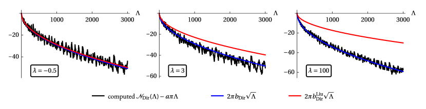
Figure 5: The Dirichlet problem for the unit disk. In this case, (1.20) may be interpreted as $\mathcal{N}_{\mathrm{Dir}}(\Lambda)-a\pi\Lambda\approx 2\pi b_{\mathrm{Dir}}\sqrt{\Lambda}$, and we compare the numerically computed left-hand sides with the right-hand sides computed using our and Liu’s expressions for $b_{\mathrm{Dir}}$. In all three images we take $\mu=1$.

The free boundary problem for the disk is treated in the same manner, the results are shown in Figure 6.

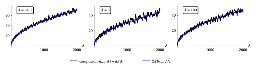
Figure 6: The free boundary counting function for the unit disk: in all three figures $\mu=1$.

Appendix C Three-dimensional examples: flat cylinders

We consider $\Omega=\Omega_{3,h}:=\mathbb{T}^{2}\times[0,h]$, where $\mathbb{T}^{2}$ is a flat square torus with side $2\pi$ and $h>0$ is the height of the cylinder, so that $\operatorname{Vol}_{3}(\Omega)=(2\pi)^{2}h$ and $\operatorname{Vol}_{2}(\partial\Omega)=8\pi^{2}$. We can once again separate variables by first setting

$$u(x^{1},x^{2},x^{3})=\operatorname{grad}\psi_{1}(x^{1},x^{2},x^{3})+\operatorname{curl}\left(\mathbf{z}\,\psi_{2}(x^{1},x^{2},x^{3})\right)+\operatorname{curl}\operatorname{curl}\left(\mathbf{z}\,\psi_{3}(x^{1},x^{2},x^{3})\right),$$ (C.1)

where the $\psi_{j}$ are scalar potentials, and $\mathbf{z}$ is the coordinate vector in the direction of $x^{3}$. Once again, it is easy to see that each potential $\psi_{j}$ satisfies (B.2), (B.3), with

$$\omega_{3,\Lambda}:=\omega_{2,\Lambda}.$$ (C.2)

The general solutions of (B.2) are now

$$\begin{split}\psi_{j}(x^{1},x^{2},x^{3})=\sum_{(k_{1},k_{2})\in\mathbb{Z}^{2}}&c_{j,k_{1},k_{2},+}\exp\left(\mathrm{i}\left(k_{1}x^{1}+k_{2}x^{2}+\sqrt{\omega_{j,\Lambda}-k_{1}^{2}-k_{2}^{2}}\ x^{3}\right)\right)\\ +&c_{j,k_{1},k_{2},-}\exp\left(\mathrm{i}\left(k_{1}x^{1}+k_{2}x^{2}-\sqrt{\omega_{j,\Lambda}-k_{1}^{2}-k_{2}^{2}}\ x^{3}\right)\right).\end{split}$$ (C.3)

Substitution of (C.1), (B.3), (C.2), and (C.3) into the boundary conditions at $x^{3}=0$ and $x^{3}=h$ leads to some secular equations which, as it turns out, depend only on the values of

$$K:=k_{1}^{2}+k_{2}^{2}\in\mathbb{N}\cup\{0\}$$

rather than on the values of $k_{1},k_{2}$ themselves; we therefore only need to consider the values of $K$ with $\Sigma_{2}(K)>0$ where

$$\Sigma_{2}(K):=\#\left\{(k_{1},k_{2})\in\mathbb{Z}^{2}:k_{1}^{2}+k_{2}^{2}=K\right\}$$

is the sum of squares function. Each solution $\Lambda>0$ of a secular equation corresponding to such a $K$ will be an eigenvalue of multiplicity $\Sigma_{2}(K)$.

The results of our computations in the Dirichlet case are collated in Figure 7 and in the free boundary case in Figure 8.

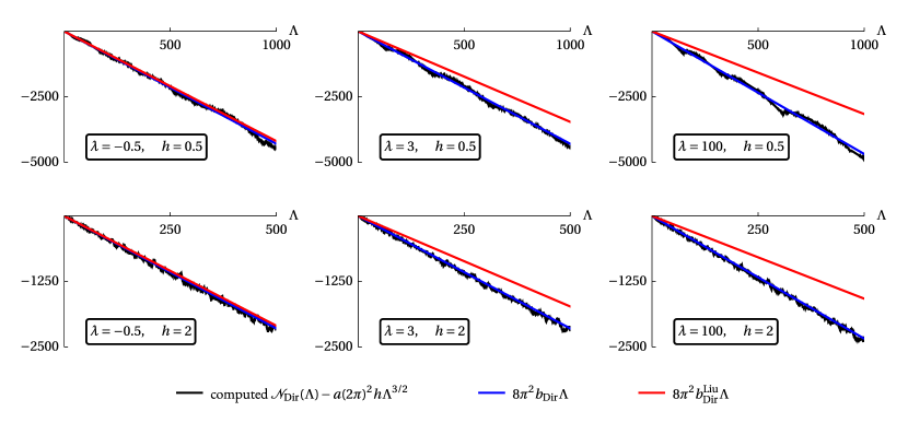
Figure 7: The Dirichlet problem for flat cylinders. In all images $\mu=1$.

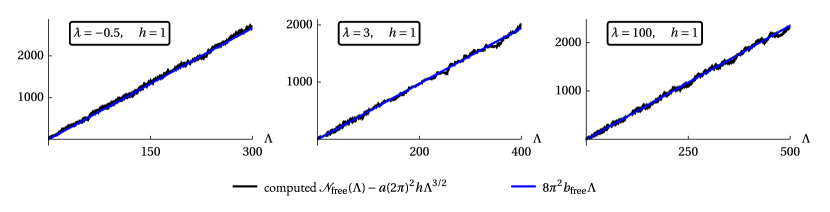
Figure 8: The free boundary problem for flat cylinders. In all images $\mu=1$.

Appendix D Second Weyl coefficients in odd dimensions: proof of Theorem 1.10

This appendix is devoted to the proof of Theorem 1.10. We will prove (1.29) and (1.30) separately, in §D.1 and §D.2 respectively, by explicitly evaluating the integrals in the right-hand sides of (1.27) and (1.28).

In this appendix we denote complex variables by

$$w=t+\mathrm{i}s,\qquad t,s\in\mathbb{R}.$$

§D.1.  Dirichlet case: proof of (1.29)

We begin by observing that, by performing a change of variable $t=\tau^{-2}$, one obtains

$$\int\limits_{\sqrt{\alpha}}^{1}\tau^{2k-1}\arctan\left(\sqrt{(1-\alpha\tau^{-2})\left(\tau^{-2}-1\right)}\right)\mathrm{d}\tau=\frac{1}{2}\int\limits_{1}^{1/\alpha}\frac{\arctan\left(\sqrt{(1-\alpha t)\left(t-1\right)}\right)}{t^{k+1}}\mathrm{d}t\,.$$

Therefore, proving (1.29) reduces to establishing the following

Lemma D.1.

For $k=1,2,\ldots$ we have

$$\frac{2k}{\pi}\int\limits_{1}^{1/\alpha}\frac{\arctan\left(\sqrt{(1-\alpha t)\left(t-1\right)}\right)}{t^{k+1}}\mathrm{d}t=\left.\frac{1}{k!}\frac{\mathrm{d}^{k}}{\mathrm{d}t^{k}}\left(\frac{2t-\frac{\alpha+1}{\alpha}}{t-\frac{\alpha+1}{\alpha}}\frac{1}{\sqrt{(1-\alpha t)(1-t)}}\right)\right|_{t=0}-\left(\frac{\alpha}{\alpha+1}\right)^{k}\,.$$ (D.1)

Proof.

The task at hand is to evaluate the integral

$$\mathcal{I}_{k}:=\int\limits_{1}^{1/\alpha}\frac{\arctan\left(\sqrt{(1-\alpha t)\left(t-1\right)}\right)}{t^{k+1}}\mathrm{d}t$$

for $k\in\mathbb{N}$. Observing that the inverse tangent turns to zero at the endpoints of the interval of integration and integrating by parts, one obtains

$$\mathcal{I}_{k}=\frac{1}{2k}\int\limits_{1}^{1/\alpha}\frac{1}{t^{k+1}}\left(\frac{2t-\frac{\alpha+1}{\alpha}}{t-\frac{\alpha+1}{\alpha}}\frac{1}{\sqrt{(1-\alpha t)\left(t-1\right)}}\right)\mathrm{d}t\,.$$

Let

$$f_{k}(w):=\frac{1}{2k}\frac{1}{w^{k+1}}\left(\frac{2w-\frac{\alpha+1}{\alpha}}{w-\frac{\alpha+1}{\alpha}}\frac{1}{\sqrt{(1-\alpha w)\left(w-1\right)}}\right),\qquad w\in\mathbb{C}.$$

It is easy to see that the function $f_{k}$ with branch cut $[1,\alpha^{-1}]$ is holomorphic in a neighbourhood of $[1,\alpha^{-1}]$ and meromorphic in $\mathbb{C}\setminus[1,\alpha^{-1}]$ with poles at

$$w=0\quad(\text{of order }k+1),\qquad w=1+\alpha^{-1}\quad(\text{of order }1)\,.$$

We choose the branch of the square root so that it is positive above the branch cut and negative below the branch cut. Note that the poles are not on the branch cut.

Let $\Gamma_{\epsilon}$ be a negatively oriented (clockwise) dog-bone contour around $[1,\alpha^{-1}]$, see Figure 9. Then

$$\mathcal{I}_{k}=\frac{1}{2}\,\lim_{\epsilon\to 0}\int_{\Gamma_{\epsilon}}f_{k}(w)\,dw\,.$$ (D.2)

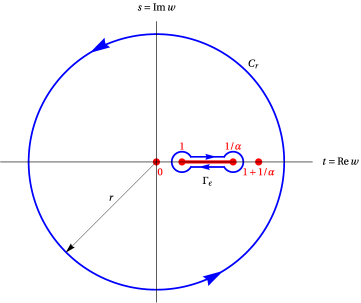
Figure 9: The contour of integration for the Dirichlet problem. The two small circles centred at $1$ and $1/\alpha$ have radius $\epsilon$.

Let $C_{r}$ be a positively oriented (counterclockwise) circular curve of radius $r$, see Figure 9, with $r>1+\alpha^{-1}$. Then by Cauchy’s Residue Theorem we have

$$\int_{\Gamma_{\epsilon}\cup C_{r}}f_{k}(w)\,dw=2\pi\mathrm{i}\left(\mathrm{Res}(f_{k},0)+\mathrm{Res}(f_{k},1+\alpha^{-1})\right)\,,$$ (D.3)

so that, combining (D.2) and (D.3), we obtain

$$\mathcal{I}_{k}=\pi\mathrm{i}\left(\mathrm{Res}(f_{k},0)+\mathrm{Res}(f_{k},1+\alpha^{-1})+\mathrm{Res}(f_{k},\infty)\right)\,.$$ (D.4)

Straightforward calculations give us

$$\mathrm{Res}(f_{k},0)=\frac{1}{2k\mathrm{i}}\frac{1}{k!}\left.\frac{\mathrm{d}^{k}}{\mathrm{d}t^{k}}\left(\frac{2t-\frac{\alpha+1}{\alpha}}{t-\frac{\alpha+1}{\alpha}}\frac{1}{\sqrt{(1-\alpha t)(1-t)}}\right)\right|_{t=0}\,,$$ (D.5)

$$\mathrm{Res}(f_{k},1+\alpha^{-1})=-\frac{1}{2k\mathrm{i}}\,\left(\frac{\alpha}{\alpha+1}\right)^{k}\,,$$

$$\mathrm{Res}(f_{k},\infty)=0\,.$$ (D.6)

Here we used that $\sqrt{(1-\alpha t)(t-1)}=\mathrm{i}\sqrt{(1-\alpha t)(1-t)}$ for $t<1$, and that $\left.\sqrt{(1-\alpha t)(t-1)}\right|_{t=1+\alpha^{-1}}=-\mathrm{i}$.

Substituting (D.5)–(D.6) into (D.4) we arrive at (D.1). ∎

§D.2.  Free boundary case: proof of (1.30)

As above, we observe that by performing a change of variable $t=\tau^{-2}$ one obtains

$$\int\limits_{\sqrt{\alpha}}^{1}\tau^{2k-1}\arctan\left(\frac{\left(\tau^{-2}-2\right)^{2}}{4\sqrt{(1-\alpha\tau^{-2})\left(\tau^{-2}-1\right)}}\right)\mathrm{d}\tau=\frac{1}{2}\int\limits_{1}^{1/\alpha}\frac{\arctan\left(\frac{\left(t-2\right)^{2}}{4\sqrt{(1-\alpha t)\left(t-1\right)}}\right)}{t^{k+1}}\mathrm{d}t\,.$$ (D.7)

We have

Lemma D.2.

For $k=1,2,\ldots$ we have

$$\begin{split}&\qquad\frac{4k}{\pi}\int\limits_{1}^{1/\alpha}\frac{\arctan\left(\frac{\left(t-2\right)^{2}}{4\sqrt{(1-\alpha t)\left(t-1\right)}}\right)}{t^{k+1}}\mathrm{d}t\\ &=-\frac{8}{k!}\left.\frac{\mathrm{d}^{k}}{\mathrm{d}t^{k}}\left(\frac{(t-2)(2\alpha t^{2}+(\alpha-3)t+2(1-\alpha))}{t^{3}-8t^{2}+8(3-2\alpha)t+16(\alpha-1)}\left(\frac{1}{\sqrt{(1-\alpha t)\left(1-t\right)}}+\frac{4}{(t-2)^{2}}\right)\right)\right|_{t=0}\\ &+2^{3-k}+2(1-\alpha^{k})-4\gamma_{R}^{-2k}.\end{split}$$ (D.8)

Proof.

The task at hand is to evaluate the integral

$$\widetilde{\mathcal{I}}_{k}:=\int\limits_{1}^{1/\alpha}\frac{\arctan\left(\frac{\left(t-2\right)^{2}}{4\sqrt{(1-\alpha t)\left(t-1\right)}}\right)}{t^{k+1}}\mathrm{d}t$$ (D.9)

for $k\in\mathbb{N}$.

In what follows, we assume, for simplicity, that $\alpha\neq\frac{1}{2}$ (this corresponds to $\lambda\neq 0$). The case $\alpha=\frac{1}{2}$ can be handled in a similar fashion.

Observing that the inverse tangent tends to $\frac{\pi}{2}$ at the endpoints of the interval of integration and integrating by parts, one obtains

$$\widetilde{\mathcal{I}}_{k}=\frac{\pi}{2k}(1-\alpha^{k})-\frac{2}{k}\int\limits_{1}^{1/\alpha}\frac{1}{t^{k+1}}\left(\frac{(t-2)(2\alpha t^{2}+(\alpha-3)t+2(1-\alpha))}{R_{\alpha}(t)}\frac{1}{\sqrt{(1-\alpha t)\left(t-1\right)}}\right)\mathrm{d}t\,,$$ (D.10)

where $R_{\alpha}$ is defined in accordance with (1.23). Hence, evaluating (D.9) reduces to evaluating

$$\widetilde{\mathcal{J}}_{k}:=\int\limits_{1}^{1/\alpha}\frac{1}{t^{k+1}}\left(\frac{(t-2)(2\alpha t^{2}+(\alpha-3)t+2(1-\alpha))}{R_{\alpha}(t)}\frac{1}{\sqrt{(1-\alpha t)\left(t-1\right)}}\right)\mathrm{d}t\,.$$ (D.11)

Let

$$\widetilde{f}_{k}(w):=\frac{1}{w^{k+1}}\left(\frac{(w-2)(2\alpha w^{2}+(\alpha-3)w+2(1-\alpha))}{R_{\alpha}(w)}\frac{1}{\sqrt{(1-\alpha w)\left(w-1\right)}}\right),$$ (D.12)

where we choose the branch of the square root in such a way that on the upper side of the branch cut $[0,\alpha^{-1}]$ we have $\sqrt{(1-\alpha w)\left(w-1\right)}>0$. It is easy to see that the function $\widetilde{f}_{k}$ is holomorphic in

$$\mathbb{C}\setminus\left(\{0\}\cup\{w_{j},\ j=1,2,3\}\cup[0,\alpha^{-1}]\right),$$

with poles at

$$w=0\quad(\text{of order }k+1),\qquad w=w_{j},\ j=1,2,3,\quad(\text{of order }1)\,,$$

where the $w_{j}$, $j=1,2,3$, are the roots $R_{\alpha}(w)$, with $0<w_{1}<1$ — recall the discussion from Remark 1.7.

The nature of the other two roots $w_{j}$, $j=2,3$, depends on $\alpha$. Let $\alpha^{*}\in(0,1)$ be the unique real root of

$$\alpha^{3}-\frac{107}{64}\alpha^{2}+\frac{31}{32}\alpha-\frac{11}{64}=0.$$

Then we have the three cases [RaBa-95]:

1. for $0<\alpha<\alpha^{*}$ there are two complex-conjugate roots $w_{2}=\overline{w_{3}}$, $\operatorname{Im}w_{2}>0$;

2. for $\alpha=\alpha^{*}$ there are two coinciding real roots $w_{2}=w_{3}$;

3. for $\alpha^{*}<\alpha<1$ there are two distinct real roots $w_{2}<w_{3}$.

We will carry out the proof for the case (i); the other two cases are analogous, and lead to the same final result.

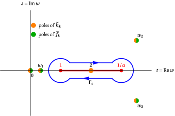
Figure 10: The contour of integration for the free boundary problem.

Let $\Gamma_{\epsilon}$ be a dog-bone contour as in Figure 10. Then

$$\widetilde{\mathcal{J}}_{k}=\frac{1}{2}\lim_{\epsilon\to 0^{+}}\int_{\Gamma_{\epsilon}}\widetilde{f}_{k}(w)\,\mathrm{d}w\,.$$

Hence, since the function $\widetilde{f}_{k}$ is regular at infinity, Cauchy’s Residue Theorem gives us

$$\widetilde{\mathcal{J}}_{k}=\pi\mathrm{i}\left(\mathrm{Res}(\widetilde{f}_{k},0)+\sum_{j=1}^{3}\operatorname{Res}(\widetilde{f}_{k},w_{j})\right)\,.$$ (D.13)

From (D.12) we immediately obtain

$$\mathrm{Res}(\widetilde{f}_{k},0)=-\frac{\mathrm{i}}{k!}\left.\frac{\mathrm{d}^{k}}{\mathrm{d}t^{k}}\left(\frac{(t-2)(2\alpha t^{2}+(\alpha-3)t+2(1-\alpha))}{R_{\alpha}(t)}\frac{1}{\sqrt{(1-\alpha t)\left(1-t\right)}}\right)\right|_{t=0}\,.$$ (D.14)

In what follows, we evaluate

$$\operatorname{Res}(\widetilde{f}_{k},w_{2})+\operatorname{Res}(\widetilde{f}_{k},w_{3})-\operatorname{Res}(\widetilde{f}_{k},w_{1})$$ (D.15)

and

$$2\operatorname{Res}(\widetilde{f}_{k},w_{1})\,.$$ (D.16)

separately and then add the results together.

Let us start with (D.15). In view of the equivalence between (1.25) and (1.26), and our choice of branch of the square root, it is not hard to check that

$$\left.\sqrt{(1-\alpha w)\left(w-1\right)}\right|_{w=w_{1}}=\frac{\mathrm{i}}{4}(w_{1}-2)^{2},$$ (D.17)

$$\left.\sqrt{(1-\alpha w)\left(w-1\right)}\right|_{w=w_{j}}=-\frac{\mathrm{i}}{4}(w_{j}-2)^{2},\qquad j=2,3\,.$$

Hence, one can recast (D.15) as

$$\operatorname{Res}(\widetilde{f}_{k},w_{2})+\operatorname{Res}(\widetilde{f}_{k},w_{3})-\operatorname{Res}(\widetilde{f}_{k},w_{1})=\sum_{j=1}^{3}\operatorname{Res}(\widetilde{h}_{k},w_{j}),$$ (D.18)

where

$$\widetilde{h}_{k}(w):=\frac{4\mathrm{i}}{w^{k+1}}\left(\frac{2\alpha w^{2}+(\alpha-3)w+2(1-\alpha)}{(w-2)R_{\alpha}(w)}\right).$$ (D.19)

Now, $\widetilde{h}_{k}$ is a meromorphic function regular at infinity, with simple poles at $w=2$ and $w=w_{j}$, $j=1,2,3$, and a pole of order $k+1$ at $w=0$. Therefore, Cauchy’s Residue Theorem implies

$$\sum_{j=1}^{3}\operatorname{Res}(\widetilde{h}_{k},w_{j})=-\operatorname{Res}(\widetilde{h}_{k},0)-\operatorname{Res}(\widetilde{h}_{k},2)\,.$$ (D.20)

Combining (D.20) and (D.18) with account of (D.19), we obtain

$$\begin{split}&\operatorname{Res}(\widetilde{f}_{k},w_{2})+\operatorname{Res}(\widetilde{f}_{k},w_{3})-\operatorname{Res}(\widetilde{f}_{k},w_{1})\\ &=-\frac{4\mathrm{i}}{k!}\frac{\mathrm{d}^{k}}{\mathrm{d}t^{k}}\left.\left(\frac{2\alpha t^{2}+(\alpha-3)t+2(1-\alpha)}{(t-2)R_{\alpha}(t)}\right)\right|_{t=0}+\frac{\mathrm{i}}{2^{k}}\,.\end{split}$$ (D.21)

Finally, let us deal with (D.16). Using the fact that $w=w_{1}$ satisfies (1.25) and the elementary Vieta’s formulae

$$w_{1}+w_{2}+w_{3}=8,\qquad w_{1}w_{2}w_{3}=-16(\alpha-1),$$

one can establish via a straightforward calculation that

$$w_{1}(w_{1}-w_{2})(w_{1}-w_{3})(w_{1}-2)=16\left(2\alpha w_{1}^{2}+(\alpha-3)w_{1}+2(1-\alpha)\right)\,.$$ (D.22)

Formulae (D.17) and (D.22) imply

$$2\operatorname{Res}(\widetilde{f}_{k},w_{1})=-\frac{\mathrm{i}}{2w_{1}^{k}}\,.$$ (D.23)

Substituting (D.14), (LABEL:eq:proofIkfreeEq18) and (D.23) into (D.13) and then into (D.11) we obtain

$$\begin{split}\widetilde{\mathcal{I}}_{k}=&-\frac{2\pi}{k\,k!}\left.\frac{\mathrm{d}^{k}}{\mathrm{d}t^{k}}\left(\frac{(t-2)(2\alpha t^{2}+(\alpha-3)t+2(1-\alpha))}{R_{\alpha}(t)}\left(\frac{1}{\sqrt{(1-\alpha t)\left(1-t\right)}}+\frac{4}{(t-2)^{2}}\right)\right)\right|_{t=0}\\ &+\frac{2\pi}{k2^{k}}+\frac{\pi}{2k}(1-\alpha^{k})-\frac{\pi}{kw_{1}^{k}}\,.\end{split}$$ (D.24)

Formula (D.8) now follows from (D.24) after rescaling and minimal simplifications with account of $w_{1}=\gamma_{R}^{2}$. ∎

Lemma D.2 and (D.7) immediately imply (1.30).

References

- [ArNiPeSt-09] W. Arendt, R. Nittka, W. Peter, and F. Steiner, Weyl’s Law: spectral properties of the Laplacian in mathematics and physics, in Mathematical analysis of evolution, information, and complexity, W. Arendt and W. P. Schleich (eds.), Wiley, 2009, 1–71. DOI: 10.1002/9783527628025.ch1.
- [CaVa-20] M. Capoferri and D. Vassiliev, Spacetime diffeomorphisms as matter fields, J. Math. Phys. 61:11 (2020), 111508. DOI: 10.1063/1.5140425.
- [CaVa-22a] M. Capoferri and D. Vassiliev, Invariant subspaces of elliptic systems I: pseudodifferential projections, J. Funct. Anal. 282:8 (2022), 109402. DOI: 10.1016/j.jfa.2022.109402.
- [CaVa-22b] M. Capoferri and D. Vassiliev, Invariant subspaces of elliptic systems II: spectral theory, J. Spectr. Theory 12:1 (2022), 301–338. DOI: 10.4171/JST/402.
- [De-12] P. Debye, Zur Theorie der spezifischen Wärmen, Ann. Phys. 344:14 (1912), 789–839. DOI: 10.1002/andp.19123441404.
- [DuMaOn-60] M. Dupuis, R. Mazo, and L. Onsager, Surface specific heat of an isotropic solid at low temperatures, J. Chem. Phys. 33:5 (1960), 1452–1461. DOI: 10.1063/1.1731426.
- [Gr-86] G. Grubb, Functional calculus of pseudodifferential boundary problems. Birkhäuser, Boston (1986). DOI: 10.1007/978-1-4612-0769-6.
- [He-12] F. Hecht, New development in FreeFem++, J. Numer. Math. 20:3–4 (2012), 251–266. DOI: 10.1515/jnum-2012-0013. See also the package website at freefem.org.
- [Iv-16] V. Ivrii, 100 years of Weyl’s law, Bull. Math. Sci. 6 (2016), 379–452. DOI: 10.1007/s13373-016-0089-y.
- [KrTu-06] K. Krupchyk and J. Tuomela, The Shapiro–Lopatinskij condition for elliptic boundary value problems, LMS J. Math. Comp. 9 (2006), 287–329. DOI: 10.1112/S1461157000001285.
- [Le-92] M. Levitin, On a spectrum of a generalized Cosserat problem, C. R. Acad. Sci. Paris, Ser. I 315 (1992), 925–930.
- [LeMoSe-21] M. Levitin, P. Monk, and V. Selgas, Impedance eigenvalues in linear elasticity, SIAM J. Appl. Math. 81:6 (2021), 2433–2456. DOI: 10.1137/21M1412955.292929The published version of this paper contains a misprint in the Supplementary materials formula (SM.1.1), which has been corrected in the latest arXiv version arXiv:2103.14097.
- [Liu-21] G. Liu, Geometric invariants of spectrum of the Navier–Lamé operator, J. Geom. Analysis 31 (2021), 10164–10193. DOI: 10.1007/s12220-021-00639-8.
- [Liu-22] G. Liu, Geometric invariants of spectrum of the Navier–Lamé operator, arxiv:2007.09730v5 (2022).
- [McKSi-67] H. McKean and I. M. Singer, Curvature and the eigenvalues of the Laplacian, J. Diff. Geom. 1 (1967), 43–69. DOI: 10.4310/jdg/1214427880.
- [Mo-50] E. W. Montroll, Size effect in low temperature heat capacities, J. Chem. Phys. 18:2, 183–185 (1950). DOI: 10.1063/1.1747584.
- [MoFe-53] P. M. Morse and H. Feshbach, Methods of theoretical physics, Vol. 2, McGraw-Hill, N. Y., 1953.
- [RaBa-95] M. Rahman and J. R. Barber, Exact expressions for the roots of the secular equation for Rayleigh waves, J. Appl. Mech. 62:1 (1995), 250–252. DOI: 10.1115/1.2895917.
- [Ra-77] J. W. Strutt [ Lord Rayleigh], The Theory of Sound, 1st edition, Macmillan, London, 1877–1878.
- [Ra-85] Lord Rayleigh, On waves propagated along the plane surface of an elastic solid, Proc. Lond. Math. Soc. 17:1 (1885), 4–11. DOI: 10.1112/plms/s1-17.1.4.
- [SaVa-97] Yu. Safarov and D. Vassiliev, The asymptotic distribution of eigenvalues of partial differential operators, Amer. Math. Soc., Providence, RI, 1997. DOI: 10.1090/mmono/155. (Chapter VI Mechanical Applications of this book is freely available online at nms.kcl.ac.uk/yuri.safarov/Book/chapter6.pdf.)
- [SivW-06] C. G. Simader and W. von Wahl, Introduction to the Cosserat problem, Analysis 26 (2006), 1–7. DOI: 10.1524/anly.2006.26.1.1.
- [Va-84] D. Vassiliev [ D. G. Vasil’ev], Two-term asymptotics of the spectrum of a boundary value problem under an interior reflection of general form, Funkts. Anal. Pril. 18:4 (1984), 1–13 (Russian, full text available at Math-Net.ru); English translation in Funct. Anal. Appl. 18 (1984), 267–277. DOI: 10.1007/BF01083689.
- [Va-86] D. Vassiliev [ D. G. Vasil’ev], Two-term asymptotic behavior of the spectrum of a boundary value problem in the case of a piecewise smooth boundary, Dokl. Akad. Nauk SSSR 286:5 (1986), 1043–1046 (Russian, full text available at Math-Net.ru); English translation in Soviet Math. Dokl. 33:1 (1986), 227–230, full text available at the author’s website.
- [ViOg-04] P. C. Vinh and R. W. Ogden, On formulas for the Rayleigh wave speed, Wave Motion 39:3 (2004), 191–197. DOI: 10.1016/j.wavemoti.2003.08.004.
- [We-15] H. Weyl, Das asymptotische Verteilungsgesetz der Eigenschwingungen eines beliebig gestalteten elastischen Körpers, Rend. Circ. Mat. Palermo 39 (1915), 1–49. DOI: 10.1007/BF03015971.