A copositive framework for
analysis of hybrid Ising-classical algorithms

Abstract

Recent years have seen significant advances in quantum/quantum-inspired technologies capable of approximately searching for the ground state of Ising spin Hamiltonians. The promise of leveraging such technologies to accelerate the solution of difficult optimization problems has spurred an increased interest in exploring methods to integrate Ising problems as part of their solution process, with existing approaches ranging from direct transcription to hybrid quantum-classical approaches rooted in existing optimization algorithms. While it is widely acknowledged that quantum computers should augment classical computers, rather than replace them entirely, comparatively little attention has been directed toward deriving analytical characterizations of their interactions. In this paper, we present a formal analysis of hybrid algorithms in the context of solving mixed-binary quadratic programs (MBQP) via Ising solvers. By leveraging an existing completely positive reformulation of MBQPs, as well as a new strong-duality result, we show the exactness of the dual problem over the cone of copositive matrices, thus allowing the resulting reformulation to inherit the straightforward analysis of convex optimization. We propose to solve this reformulation with a hybrid quantum-classical cutting-plane algorithm. Using existing complexity results for convex cutting-plane algorithms, we deduce that the classical portion of this hybrid framework is guaranteed to be polynomial time. This suggests that when applied to NP-hard problems, the complexity of the solution is shifted onto the subroutine handled by the Ising solver.

1 Introduction

Recent years have seen significant advances in quantum and quantum-inspired Ising solvers, such as quantum annealers [johnson2011quantum], quantum approximate optimization circuits [farhi2014quantum], or coherent Ising machines [honjo2021100]. These are devices/methodologies designed to heuristically compute solutions of optimization problems of the form: $\min_{z\in\{-1,1\}^{n}}\sum_{i,j}J_{i,j}z_{i}z_{j}+\sum_{i}h_{i}z_{i}$, where $J_{i,j},\,h_{i}$ are real coefficients and $z_{i}\in\{-1,1\}$ are discrete variables to be optimized over. The promise of leveraging such technologies to speed up the solution of complex optimization problems has spurred many researchers to explore how Ising solvers can be applied to problems in various domains.

A standard approach has emerged where an optimization problem is directly transcribed into an Ising problem, and the returned solution is taken at face value or with minimal post-processing. While this method works well for problems that organically have an Ising form, sequences of reformulations can result in ill-conditioning of the problem in terms of the number of additional variables, the coupling strengths, and the optimization landscape. Most unnaturally, however, relying solely on the Ising solver means forgoing the advantages of already powerful classical computers.

In an effort to introduce meaningful interplay between classical and quantum computers, a few authors have proposed decomposition methods based on the Alternating Direction Method of Multipliers (ADMM), [gambella2020multiblock], or Benders Decomposition (BD), [chang2020hybrid, zhao2021hybrid, paterakis2021hybrid]. Critically, when ADMM is applied to non-convex problems, it is not guaranteed to converge. When it does, it is often to a local optimum without convergence guarantees to global optimality. On the other hand, while it may be possible to derive optimality guarantees using BD, proving convergence typically relies on an exhaustive search through the “complicating variables”. This makes it unclear whether such an algorithmic scaffold is primed to take advantage of speed-ups that the Ising solver may offer.

Contributions

Our work is motivated by the desire to rigorously analyze the interplay between classical and quantum machines in hybrid algorithms. Such analysis is a cornerstone for articulating and setting standards for hybrid quantum-classical optimization algorithms. Specifically, we espouse convergent hybrid quantum-classical algorithms that (1) use Ising solvers as a primitive while offering some resilience to their heuristic nature and (2) have polynomial complexity in the classical portions of the algorithm. To this end, the contribution of this paper is an algorithmic framework that satisfies these key desiderata. Concretely,

1. We revisit and prove strong duality of a result in [Burer2009] to show that the convex copositive formulation of many mixed-binary quadratic optimization problems is exact. Neglecting the challenges of working with copositive matrices, convex programs are a well-understood class of optimization problems with a wide variety of efficient solution algorithms. By reformulating mixed-binary quadratic programs as copositive programs, we open the door for hybrid-quantum classical algorithms that are based on existing convex optimization algorithms.

2. To solve the copositive programs, we propose applying a standard cutting-plane algorithm, which we modify in a novel way using a hybrid quantum-classical approach. In particular, the cutting-plane algorithm serves as a template for a solution algorithm that alternates between checking copositivity and other operations. We hybridize the algorithm by approximating the copositivity checks via discretization and solving them with an Ising solver. We show that the complexity of the portion of the algorithm handled by the classical computer has polynomial scaling. This analysis suggests that when applied to NP-hard problems, the complexity of the solution is shifted onto the subroutine handled by the Ising solver.

3. We conducted benchmarking based on the maximum clique problem to validate our theoretical claims and evaluate potential speed-ups from using a stochastic Ising solver in lieu of a state-of-the-art deterministic solver or an Ising heuristic. Results indicate that the Ising formulation of the subproblems of the hybrid algorithm is efficient versus a MIP formulation in Gurobi, and the hybrid algorithm potentially is competitive even against a non-hybridized Ising formulation of the full problem solved by simulated annealing.

We emphasize that the contribution of this work is not the copositive reformulation or a novel cutting-plane algorithm but rather the insight that these ideas are synergistic with recent advances in quantum(-inspired) computing. In particular, copositive optimization is useful for deriving and analyzing new hybrid algorithms rooted in existing convex optimization algorithms, thus filling a gap in the hybrid algorithms literature.

While preparing this manuscript, a hybrid quantum-classical method relying upon a Frank-Wolfe method was published [yurtsever2022q]. This work also leverages a similar copositive reformulation of quadratic binary optimization problems. We highlight the differences between that work and the one in our manuscript below. This manuscript considers the optimization problem class of mixed-binary quadratic programs, while in [yurtsever2022q], the authors propose their method for quadratic binary optimization problems, a subcase of the problems considered herein. Moreover, we provide proof of the exactness and strong duality for copositive/completely positive optimization stemming from the mixed-integer quadratic reformulation, addressing an open question in the field. In their manuscript, [yurtsever2022q] conjectures the results proved in this manuscript to be true. Finally, our solution method, which is based on cutting-plane algorithms, has a potential exponential speed-up in runtime compared to Frank-Wolfe algorithms.

1.1 Related Work

One dominant method for mapping optimization problems into Ising problems is through direct transcription. This process typically involves discretizing continuous variables and passing constraints into the objective through a penalty function; the returned solution is often taken at face value or with minimal post-processing to enforce feasibility. Owing to its simplicity, this process has found applications in a variety of problems, including jobshop scheduling [venturelli2016job], routing problems [harwood2021formulating], community detection [negre2020detecting], and all of Karp’s 21 NP-complete models [lucas2014ising], among others. Critically, unless a problem organically takes an Ising form, this approach often requires many auxiliary variables (spins), introduces large skews in the coupling coefficients, and can result in poor conditioning of the optimization landscape, thus limiting the problems that can be solved on near-term devices. Similarly, extending the class of applicable problem instances requires deriving increasingly complex sequences of reformulations, each of which reduces the solubility of the final reformulation. More importantly, an algorithm with minimal interactions between classical and quantum computers disregards the bountiful successes of classical computers in the past decades. This has inspired some researchers to examine how quantum computers can be used to augment classical computers instead of replacing them entirely [callison2022hybrid].

As an alternative to direct transcription, there is a burgeoning body of literature exploring the potential of decomposition methods for designing hybrid quantum-classical algorithms. These generally refer to algorithms that divide effort between a classical and quantum computer, with each computer informing the computation carried out by the other. Among these, algorithms based on the Benders Decomposition (BD) are gaining traction. BD is particularly effective for problems characterized by “complicating variables”, for which the problem becomes easy once these variables are fixed. For example, a mixed-integer linear program (MILP) becomes a linear program (LP) once the integer variables are fixed–the integers are the complicating variables. BD iterates between solving a master problem over the complicating variables and sub-problems where the complicating variables are fixed, whose solution is used to generate cuts for the master problem. Both [chang2020hybrid] and [zhao2021hybrid] consider mixed-integer programming (MIP) problems where the integer variables are linked to the continuous variables through a polyhedral constraint and leverage a reformulation where dependence on the continuous variables is expressed as constraints over the extreme rays and points of the original feasible region. Because the number of extreme rays and points may be exponentially large, the constraints are not written down in full but are iteratively generated from the solutions of the sub-problems. The master problem is an integer program consisting of these constraints and is solved using the quantum computer. Notably, the generated constraint set may be large, with the worst case being the generation of the entire constraint set, resulting in a large number of iterations. The approach in [paterakis2021hybrid] attempts to mitigate this by generating multiple cuts per iteration and selecting the most informative subset of these cuts. Instead of using the quantum computer to solve the master problem, the quantum computer is used to heuristically select cuts based on a minimum set cover or maximum coverage metric. While this may effectively reduce the number of iterations and size of the constraint set, the master problem is often an integer program that may be computationally intractable. For each of the proposed approaches, it is unclear how the complexity of the problem is distributed through the solution process For example, for [chang2020hybrid, zhao2021hybrid] the complexity might show up in the number of iterations, and for [paterakis2021hybrid] it might show up when solving the master problem. Consequently, it is ambiguous whether BD-based approaches can take advantage of a speed-up in the Ising solver, even if one were to exist.

Another decomposition that has been explored is based on the Alternating Direction Method of Multipliers (ADMM)[gambella2020multiblock]. This is an algorithm to decompose large-scale optimization problems into smaller, more manageable sub-problems [boyd2011distributed]. While originally designed for convex optimization, ADMM has shown great success as a heuristic for non-convex optimization as well, [diamond2018general], and significant progress has been made towards explaining its success in such settings [wang2019global]. In [gambella2020multiblock], the authors propose an ADMM-based decomposition with three sub-problems: the first being over just the binary variables, the second being the full problem with a relaxed copy of the binary variables, and the third being a term that ties the binary variables and their relaxed copies together. For quadratic pure-binary problems, the authors show that the algorithm converges to a stationary point of the augmented Lagrangian, which may not be a global optimizer Convergence to a global optimum is only guaranteed under the more stringent Kurdyka-Łojasiewicz conditions on the objective function [attouch2013convergence]. Unfortunately, the assumptions guaranteeing convergence to a stationary point fail in the presence of continuous variables.

A third class of decomposition proposed and implemented in the qbsolv solver is based on tabu search [BoothReinhardtEtAl2017]. qbsolv can be seen as iterating between a large-neighborhood local search (using an Ising solver) and tabu improvements to locally refine the solution (using a classical computer), where previously found solutions are removed from the search space in each iteration. During the local search phase, subsets of the variables are jointly optimized while the remaining variables are fixed to their current values. The solution found in this phase is then used to initialize the tabu search algorithm, and the process is repeated for a fixed number of iterations. Critically, it is unclear whether the algorithm is guaranteed to converge and, if so, what its optimality guarantees are. While finite convergence of tabu search is investigated in [glover2002tabu], it relies on either recency or frequency memory that ensures an exhaustive search of all potential solutions.

Another approach for purely integer programming problems is based on the computation of a Graver basis through the computation of the integer null-space of the constraint set as proposed in [alghassi2019graver]. This null-space computation is posed as a quadratic unconstrained binary optimization (QUBO) and then post-processed to obtain the Graver basis of the constraint set, a test-set of the problem. The test-set provides search directions for an augmentation-based algorithm. For a convex objective, it provides a polynomial oracle complexity in converging to the optimal solution. The authors initialize the problem by solving a feasibility-based QUBO and extend this method to non-convex objectives by allowing multiple starting points for the augmentation. The multistart procedure also alleviates the requirement for computing the complete Graver basis of the problem, which grows exponentially with the problem’s size. Considering an incomplete basis or non-convex objectives makes the Graver Augmentation Multistart Algorithm (GAMA) a heuristic for general integer programming problems, and it cannot address problems with continuous variables.

In this paper, we seek to address a gap in the literature on a rigorous theory of hybrid quantum-classical optimization. By revisiting the hidden convex structure of non-convex problems, we pave the way for hybrid algorithms based on efficient convex optimization. We show that algorithms derived through this approach inherit the straightforward analysis of convex optimization without sacrificing the potential benefits of quantum computing for non-convex problems.

While there is optimism regarding improvements to and our understanding of quantum technology in the coming decades, few expect that they will replace classical computers entirely. We believe that the method presented in this paper is an approach to algorithm design that anticipates a future where quantum computers and classical computers work in tandem. In particular, we envision a mature theory of hybrid algorithms that clearly delineates how quantum and classical computers should complement each other.

1.2 Quantum/Quantum-inspired Ising Solvers

Adiabatic quantum computing (AQC) is a quantum computation paradigm that operates by initializing a system in the ground state of an initial Hamiltonian (i.e., the optimal solution of the corresponding objective function) and slowly sweeping the system to an objective Hamiltonian. This Hamiltonian, referred to as the cost Hamiltonian, maps the objective function of the classical Ising model onto a system with as many quantum bits, or qubits, as original variables in the Ising model. The adiabatic theorem of quantum mechanics states that if the system evolution is “sufficiently slow”, the system ends up in the ground state of the desired Hamiltonian. Here, “sufficiently slow” depends on the minimum energy gap between the ground and the first excited state throughout the system evolution [albash2018adiabatic]. Since the evaluation of the minimal gap is mostly intractable, one is forced to phenomenologically “guess” the evolution’s speed, and if it is too fast, the undesired non-adiabatic transitions can occur. Additionally, real devices are plagued with various incarnations of physical noise, such as thermal fluctuations or decoherence effects, that can hamper computation. The situation is further exacerbated by the challenge of achieving dense connectivity between qubits. Densely connected problems are embedded in devices by chaining together multiple physical qubits to represent one logical qubit. The heuristic computational paradigm that encompasses the additional noise and non-quantum effects is known as Quantum Annealing (QA). [hauke2020perspectives] provides a review on QA with a focus on possible routes towards solving the open questions in the field.

An alternative paradigm to AQC is the gate-based model of quantum computing. Within the gate-based model, Variational Quantum Algorithms (VQAs) is a class of hybrid quantum-classical algorithms that can be applied to optimization [cerezo2021variational]. VQAs share a common operational principle where the “loss function” of a parameterized quantum circuit is measured on a quantum device and evaluated on a classical processor, and a classical optimizer is used to update (or “train”) the circuit’s parameters to minimize the loss. VQAs are often interpreted as a quantum analog to machine learning, leaving many similar questions open regarding their trainability, accuracy, and efficiency. Most similar in spirit to this work is a theory of variational hybrid quantum-classical algorithms proposed in [mcclean2016theory]. However, they primarily focus on algorithmic improvements to the quantum portion, with discussion of the classical optimization being limited to empirical evaluations of existing derivative-free optimization algorithms. More recently, [bittel2021training] analyzed the complexity of training VQAs, and through reductions from the maximum cut problem, showed that it is NP-hard. The analysis presented in this paper complements these prior works in developing a more complete picture of the interplay between quantum and classical computers.

The quantum approximate optimization algorithm (QAOA) is a specific instance of a VQA where the structure of the quantum circuit is the digital analog of adiabatic quantum computing [farhi2014quantum]. QAOA operates by alternating the application of the cost Hamiltonian and a mixing Hamiltonian; the number of alternating blocks is referred to as the circuit depth. For each one of the alternating steps, either mixing or cost application, a classical optimizer needs to determine how long each step should be performed, encoded as rotation angles. Optimizing the expected cost function with respect to the rotation angles is a continuous low-dimensional non-convex problem. QAOA is designed to optimize cost Hamiltonians, such as the ones derived from classical Ising problems. Performance guarantees can be derived for QAOA with well-structured problems, given that the optimal angles are found in the classical optimization step. Although approximation guarantees have not been derived for arbitrary cost Hamiltonians, even depth-one QAOA circuits have non-trivial performance guarantees for specific problems and cannot be efficiently simulated on classical computers [farhi2016quantum], thus bolstering the hope for a speed-up in near-term quantum machines. Moreover, the algorithm’s characteristics, such as relatively shallow circuits, make it amenable to be implemented in currently available noisy intermediate-scale quantum (NISQ) computers compared to other algorithms requiring fault-tolerant quantum devices [preskill2018quantum]. While QAOA’s convergence to optimal solutions is known to improve with increased circuit depth and to succeed in the infinite depth limit following its equivalence to AQC, its finite depth behavior has remained elusive due to the challenges in analyzing quantum many-body dynamics and other practical complications such as decoherence when implementing long quantum circuits, compilation issues, and hardness of the optimal angle classical problem [uvarov2021barren]. Even considering these complications, QAOA has been extensively studied and implemented in current devices [willsch2020benchmarking, harrigan2021quantum], becoming one of the most popular alternatives to address combinatorial optimization problems modeled as Ising problems using gate-based quantum computers. Several other quantum heuristics for Ising problems have been proposed, usually requiring fault-tolerant quantum computers. We direct the interested reader to a recent review on the topic [sanders2020compilation].

An alternative physical system for solving Ising problems that has emerged is coherent Ising machines (CIMs), which are optically pumped networks of coupled degenerate optical parametric oscillators. As the pump strength increases, the equilibrium states of an ideal CIM correspond to the Ising Hamiltonian’s ground states encoded by the coupling coefficients. Large-scale prototypes of CIMs have achieved impressive performance in the lab, thus driving the theoretical study of their fundamental operating principles. While significant advances have been made on this front, we still lack a clear theoretical understanding of the CIMs’ computational performance. Since a thorough understanding of the CIM is limited by our capacity to prove theorems about complex dynamic systems, near-term usage of CIMs must treat them as a heuristic rather than a device with performance guarantees [yamamoto2017coherent]. Even so, there are empirical observations that in many cases, the median complexity of solving Ising problems using CIM scales as $\exp{\sqrt{N}}$ where $N$ is the size of the problem [mohseni2022ising], making it a potential approach to solve these problems efficiently in practice. We note that there are other types of Ising machines, including classical thermal annealers (based on magnetic devices [shim2017ising], optics [pierangeli2019large], memristors [bojnordi2016memristive], and digital hardware accelerators [matsubara2020digital]), dynamical-systems solvers (based on optics [mcmahon2016fully] and electronics [chou2019analog]), superconducting-circuit quantum annealers [albash2018demonstration], and neutral atoms arrays [henriet2020quantum]. We direct the interested reader to [mohseni2022ising], which provides a recent review and comparison of various methods for constructing Ising machines and their operating principles.

Organization

In Section 2, we present notation, terminology, and the problem setting covered by our approach. In Section 3, we introduce the proposed framework, including convex reformulation via copositive programming, a high-level overview of cutting-plane algorithms, and a specific discussion of their application to copositive programming. Section 4 provides numerical experiments supporting our assertions about the proposed approach. Finally, we conclude and highlight future directions in Section LABEL:sec:conclusion.

2 Preliminaries

2.1 Notation and Terminology

In this paper, we solely work with vectors and matrices defined over the real numbers and reserve lowercase letters for vectors and uppercase letters for matrices. We will also follow the convention that a vector $x\in\mathbb{R}^{n}$ is to be treated as a column vector, i.e., equivalent to a matrix of dimension $n\times 1$. For a matrix $M$, we use $M_{i,j}$ to denote the entry in the $i$th row and $j$th column, $M_{i,*}$ denotes the entire $i$th row, and $M_{*,j}$ denotes the entire $j$th column. In the text, we frequently use block matrices with structured zero entries; we use $\cdot$ as shorthand for zero entries. We use $\mathds{1}$ to denote the all-ones vectors and ${\mathds{1}_{\{j\}}}$ to denote the $j$th standard basis vector (i.e., a vector where all entries are zero except for a 1 for the jth entry). The $p$-norm of a vector $v\in\mathbb{R}^{n}$ is defined as $\left\lVert v\right\rVert_{p}:=\left(\sum_{i=1}^{n}v_{i}^{p}\right)^{1/p}$. We reserve the letter $I$ to denote the identity matrix. For two matrices, $M$ and $N$, we use $\langle M,\,N\rangle=\text{Tr}(M^{\top}N)$ to denote the matrix inner product. Note that for two vectors, $\text{Tr}(x^{\top}y)=x^{\top}y$ because $x^{\top}y$ is a scalar, so the matrix inner product is consistent with the standard inner product on vectors. For sets, $S_{M}+S_{N}:=\{M+N\mid M\in S_{M},N\in S_{N}\}$ is their Minkowski sum, $S_{M}\cup S_{N}$ their union, and $S_{M}\cap S_{N}$ their intersection. For a cone, $\mathcal{K}$, its dual cone is defined as $\mathcal{K}^{*}=\{X\mid\langle X,\,K\rangle\geq 0,\forall K\in\mathcal{K}\}$. While we work with matrix cones in this paper, this definition of dual cones is consistent with vector cones as well. In this paper, the two cones we will work with are the cone of completely positive matrices and the cone of copositive matrices. The cone of completely positive (CP) matrices, $C^{*}$, is the set of matrices that have a factorization with entry-wise non-negative entries:

(1) $$\mathcal{C}^{*}_{n}:=\{X\in\mathbb{R}^{n\times n}\mid X=\sum_{k}x^{(k)}(x^{(k)})^{\top},\quad x^{(k)}\in\mathbb{R}^{n}_{\scriptscriptstyle\geq 0}\}$$

The cone of copositive matrices, $\mathcal{C}$, is the set of matrices defined by:

(2) $$\mathcal{C}_{n}:=\{X\in\mathbb{R}^{n\times n}\mid v^{\top}Xv\geq 0,\quad\forall v\in\mathbb{R}^{n}_{\scriptscriptstyle\geq 0}\}$$

As suggested by the notation, the cones of completely positive and copositive matrices are duals of each other. We use $S^{n}_{++}$ to denote the cone of positive definite matrices.

In this paper, we will use the terms Ising problem and quadratic unconstrained binary optimization (QUBO) interchangeably. An Ising problem is an optimization problem of the form: $\min_{z\in\{-1,1\}^{n}}\sum_{i,j}J_{i,j}z_{i}z_{j}+\sum_{i}h_{i}z_{i}$, where $J_{i,j},\,h_{i}$ are real coefficients and $z_{i}\in\{-1,1\}$ are discrete variables to be optimized over. A QUBO, which is an optimization problem of the form $\min_{x\in\{0,\,1\}^{n}}\sum_{i,j}Q_{i,j}x_{i}x_{j}$ can be reformulated as an Ising problem using the change of variable $z=2x-\mathds{1}$. This translates to coefficients in the Ising problem $J_{i,j}=\frac{1}{4}Q_{i,j}$, $h_{i}=\frac{1}{2}\sum_{j}Q_{i,j}$, and a constant offset of $\frac{1}{4}\sum_{i,j}Q_{i,j}$.

2.2 Problem Setting

In this paper, we consider mixed-binary quadratic programs (MBQP) of the form: x ∈R^nx^⊤Q x + 2 c^⊤x Ax = b,  A ∈R^m×n,   b ∈R^m x ≥0 x_j ∈{0, 1},  j ∈B where the set $B\subseteq\{1,\ldots,{n}\}$ indexes which of the $n$ variables are binary. This is a general class of problems that encompasses problems including QUBOs, standard quadratic programming, the maximum stable set problem, and the quadratic assignment problem. Because mapping to an Ising problem can also be equivalently expressed as a QUBO, many problems tackled with Ising solvers thus far pass through a formulation similar to the form of Problem (2.2). Using the result in [Burer2009, Sec. 3.2], the formulation considered in this paper can be extended to include constraints of the form $x_{i}x_{j}=0$ that force at least one of $x_{i}$ or $x_{j}$ to be zero, i.e., complementarity constraints. For ease of notation, this extension is left out of the present discussion.

3 Proposed Methodology

In this section, we will discuss our proposed methodology for solving Problem (2.2) given access to Ising solvers. Our result relies on a convex reformulation of Problem (2.2) as a copositive program. Leveraging convexity, we propose to solve the problem using cutting-plane algorithms. These belong to a broad class of convex optimization algorithms whose standard components give rise to a natural separation between the role of the Ising solver versus a classical computer.

We first state Burer’s exact reformulation of Problem (2.2) as a completely positive program and its dual copositive program. We then show that under mild conditions (i.e., feasibility and boundedness) of the original MBQP, the copositive and completely positive programs exhibit strong duality. We will then introduce the class of cutting-plane algorithms and summarize the complexity guarantees of several well-known variants. Finally, we explicitly show how cutting-plane algorithms can be used to solve copositive optimization problems given a copositivity oracle and discuss how to implement a copositivity oracle using an Ising solver.

3.1 Convex formulation as a copositive program

In his seminal work, Burer showed that MBQPs can be represented exactly as completely positive programs of the form: X ∈R^n×n,   x ∈R^n⟨(Q c c⊤⋅ ) ,   (X x x⊤1 ) ⟩ ⟨(⋅ 12Ai, *⊤12Ai, *⋅ ) ,   (X x x⊤1 ) ⟩ = b_i,   i = 1, …, m ⟨(A⊤i, *Ai, *⋅ ⋅ ⋅ ) ,   (X x x⊤1 ) ⟩ = b^2_i,   i = 1, …, m ⟨(-1{j}1{j}⊤121{j}121{j}⊤⋅ ) ,   (X x x⊤1 ) ⟩ = 0,   j ∈B (X x x⊤1 ) ∈C^*_n+ 1, where exactness means that Problems (2.2) and (3.1) have the same optimal objective and for an optimal solution, $(x^{*},X^{*})$, of (3.1), $x^{*}$ lies within the convex hull of optimal solutions for (2.2) [Burer2009, Theorem 2.6]. Similar to semi-definite programming (SDP) relaxations, the completely positive formulation involves lifting the variables in (2.2) to a matrix variable representing their first and second-degree monomials, making the objective function and constraints linear. Unlike SDP relaxations, however, the complete positivity constraint is sufficient for ensuring that the feasible region of (3.1) is exactly the convex hull of the feasible region of (2.2). This distinction is what ensures that the optimal value of (3.1) is exactly that of (2.2), whereas for an SDP relaxation, the optimal solution may lie outside of the convex hull of (2.2), resulting in a lower objective value (i.e., a relaxation gap).

Taking the dual of (3.1) yields a copositive optimization problem of the form [boyd2004convex, Section 5.9]: μ, λ, γγ+ ∑_i = 1^m μ^(lin)_i b_i + μ^(quad)_i b_i^2 M(μ, λ, γ) ∈C_n+ 1, where

(2) $$M(\mu,\lambda,\gamma):= {\scriptsize\begin{pmatrix}{Q}&{c}\\ {c}^{\top}&{\cdot}\end{pmatrix}}-\sum_{i=1}^{{m}}\mu^{\text{(lin)}}_{i}{\scriptsize\begin{pmatrix}\cdot&\frac{1}{2}A_{i,*}^{\top}\\ \frac{1}{2}A_{i,*}&\cdot\end{pmatrix}}-\sum_{i=1}^{{m}}\mu^{\text{(quad)}}_{i}{\scriptsize\begin{pmatrix}A^{\top}_{i,*}A_{i,*}&\cdot\\ \cdot&\cdot\end{pmatrix}}$$

$$-\sum_{j\in B}\lambda_{j}{\scriptsize\begin{pmatrix}{-{\mathds{1}_{\{j\}}}{\mathds{1}_{\{j\}}}^{\top}}&{\frac{1}{2}{\mathds{1}_{\{j\}}}}\\ {\frac{1}{2}{\mathds{1}_{\{j\}}}}^{\top}&{\cdot}\end{pmatrix}}-\gamma{\scriptsize\begin{pmatrix}\cdot&\cdot\\ \cdot&1\end{pmatrix}}$$

is a parametrized linear combination of the constraint matrices. The dual copositive program has a linear objective and a single copositivity constraint–this is a convex optimization problem. While weak duality always holds between an optimization problem and its dual, strong duality is not generally guaranteed. Showing that strong duality holds is critical for ensuring convergence of specific optimization algorithms and exactness when solving the dual problem as an alternative to solving the primal.

Theorem 3.1 (Strong Duality).

If Problem (2.2) is feasible with bounded feasible region, then strong duality holds between Problems (3.1) and (3.1) (i.e., $\min\eqref{eq:CPP}=\max\eqref{eq:COP}$).

Proof 3.2 (Proof Sketch).

Our proof proceeds by first showing strong duality between the alternative representation of (3.1) (using a homogenized formulation of the equality constraints) and its dual. By showing that the optimal value of (3.1) is lower-bounded by the optimal value of this homogenized dual problem, we can sandwich the optimal values of Problems (3.1) and (3.1) by those of a primal-dual pair that has been shown to exhibit strong duality. The complete proof of this result is provided in Appendix LABEL:subsec:strong_dual.

In prior work, characterization of the duality gap between Problems (3.1) and (3.1) has remained elusive because the feasible region of Problem (3.1) never has an interior, thus prohibiting straightforward application of Slater’s constraint qualification. This result is significant because it shows that under mild conditions, the copositive formulation is exact. This means that the optimal values of Problems (2.2) and (3.1) are equivalent, so solving Problem (3.1) is a valid alternative to solving Problem (2.2). The framework developed in this paper will ultimately produce approximate solutions for Problems (3.1) and (3.1), which we anticipate can be used to speed up the solution process of a purely classical solver for (2.2). For example, the heuristic solutions or cuts used to generate them might be used to warm-start or initialize a purely classical solver.

While Problems (3.1) and (3.1) are both convex, neither resolve the difficulty of Problem (2.2) as even checking complete positivity (resp. copositivity) of a matrix is NP-hard (resp. co-NP-complete) [murty1987some]. Instead, they should be viewed as “packaging” the complexity of the problem entirely in the copositivity/complete positivity constraint. There are a number of classical approaches for (approximately) solving copositive/completely positive programs directly, such as the sum of squares hierarchy [Parrilo2000, lasserre2001global], feasible descent method in the completely positive cone, approximations of the copositive cone by a sequence of polyhedral inner and outer approximations, among others [dur2021conic, burer2012copositive, dur2010copositive]. In this paper, we will exploit the innate synergy between checking copositivity, which is most naturally posed as a quadratic minimization problem, and solving Ising problems. This perspective is suggestive of a hybrid quantum-classical approach where the quantum computer is responsible for checking feasibility (i.e., the “hard part”) of the copositive program while the classical computer directs the search towards efficiently reducing the search space.

3.2 Cutting-Plane/Localization Algorithms

Cutting-plane/localization algorithms are convex optimization algorithms that divide labor between checking feasibility, abstracted as a separation oracle, and optimization of the objective . In this section, we provide a high-level overview of each algorithmic step and summarize both the runtime and oracle complexities of several well-known variants; these complexity measures will ultimately correspond to the complexity of the sub-routine handled by the classical computer and the number of calls to the Ising solver, respectively.

While cutting-plane algorithms are often used to solve both constrained and unconstrained optimization problems, they are generally evaluated in terms of their complexity when solving the feasibility problem.

Definition 3.3 (Feasibility Problem).

For a set of interest $S\subset\mathbb{R}^{{m}}$, which can only be accessed through a separation oracle, the feasibility problem is concerned with either finding a point in the set $x\in S$ or proving that $S$ does not contain a ball of radius $r$.

Definition 3.4 (Separation Oracle).

A separation oracle for a set $S$, $\texttt{Oracle}_{S}(\cdot)$ takes as input a point $x\in\mathbb{R}^{{m}}$ and either returns True if $x\in S$ or a separating hyperplane if $x\not\in S$. A separating hyperplane is defined by a vector, ${a}\in\mathbb{R}^{{m}}$ and scalar ${b}\in\mathbb{R}$ such that ${a}^{\top}s\leq{b}$ for all $s\in S$ but ${a}^{\top}x\geq{b}$.

The feasibility problem formulation is non-restrictive because these methods can be readily adapted to solving quasi-convex optimization problems with only a simple modification to the separation oracle. In particular, if the separation oracle indicates feasibility and returns a vector $g\in\mathbb{R}^{m}$ where any vectors $x,y\in\mathbb{R}^{m}$ with $f(y)<f(x)$ implies that $g^{\top}y\geq g^{\top}x$, this serves as a separating hyperplane for the subset of the feasible region that has a better objective than the test point. If $f$ is subdifferentiable, any subgradient $g\in\partial f(x)$ satisfies this condition, and for Problem (3.1), choosing $g$ as the objective’s coefficient vector is sufficient.

Although there are many variations of cutting-plane algorithms, at a high level, they follow a standard template that consists of alternating between checking feasibility of a test point, updating an outer approximation of the feasible region, and judiciously selecting the next test point. This standard template is summarized in Algorithm 1. An overview of the Ellipsoid algorithm is included in the Appendix as a representative example of cutting-plane algorithms, and we direct the interested reader to the references listed in Table 1 for specific implementation details. By choosing subsequent test points to be the center of the outer approximation, the algorithm is guaranteed to make consistent progress in reducing the search space (where the metric of progress may also vary across cutting-plane algorithms). Intuitively, cutting plane algorithms can be considered a high-dimensional analog of binary search. We note that the requirement $\text{Vol}(S_{0})\leq R$ means that the initial set must be bounded. While this is a standard assumption in the cutting-plane literature, finding such an $S_{0}$ may be non-trivial. Procedurally, one may construct a bounded outer approximation using a linear program as in Step 1, Algorithm 1 of [sivaramakrishnan2007properties].

Input: $S_{0}\subseteq\mathbb{R}^{{m}}$ (Initial Set) with $\texttt{Vol}(S_{0})\leq R$

Output: $x\in S$ or False if S does not contain a ball of volume $r$

$x\leftarrow\texttt{Center}(S_{0})$;

$k\leftarrow 0$;

while Oracle(x) is not True and $\texttt{Vol}(S_{k})\geq r$ do

       $S_{k+1}\leftarrow\texttt{Add\_Cut}(S_{k},\texttt{Oracle}(x))$;

       $x\leftarrow\texttt{Center}(S_{k+1})$;

       $k\leftarrow k+1$;

      

end while

if Oracle(x) is True then

       return $x$;

      

else

       return False;

      

end if

Algorithm 1 Cutting-plane meta-algorithm (feasibility problem)

A number of well-known variants of cutting-plane algorithms are summarized in Table 1. Differences across instantiations of cutting-plane algorithms vary in how subsequent test points are chosen, how the outer approximation is updated, and how progress in decreasing the outer approximation’s size is measured. Each of the surveyed variants strikes a different balance between the computational effort needed to compute a good center versus the resolution used to represent the outer approximation. Critically, except for the Center of Gravity method, all cutting-plane algorithms summarized in Table 1 have a polynomial complexity in the dimension of the optimization variables in terms of both oracle queries and total runtime excluding the oracle calls (i.e., the total complexity of adding the cuts and generating test points). This suggests that if a cutting-plane algorithm were applied to Problem (3.1), the complexity of the problem is offloaded onto the separation oracle; this is the subroutine we propose to handle using an Ising solver.

Name	Oracle Queries	Total runtime (excluding oracle queries)	References
Center of Gravity	$\mathcal{O}({{m}}\log(\frac{R}{r}))$	#P-hard [rademacher2007approximating]	[levin1965algorithm]
Ellipsoid	$\mathcal{O}({{m}}^{2}\log({{m}}\frac{R}{r}))$	$\mathcal{O}({{m}}^{4}\log({{m}}\frac{R}{r}))$	[shor1977cut, yudin1976evaluation, khachiyan1980polynomial]
Inscribed Ellipsoid	$\mathcal{O}({{m}}\log({{m}}\frac{R}{r}))$	$\mathcal{O}(({{m}}\log({{m}}\frac{R}{r}))^{4.5})$	[khachiyan1988method, nesterov1989self]
Volumetric Center	$\mathcal{O}({{m}}\log({{m}}\frac{R}{r}))$	$\mathcal{O}({{m}}^{1+\omega}\log({{m}}\frac{R}{r}))$	[vaidya1989new]
Analytic Center	$\mathcal{O}({{m}}\log^{2}({{m}}\frac{R}{r}))$	$\mathcal{O}({{m}}^{1+\omega}\log^{2}({{m}}\frac{R}{r})+({{m}}\log({{m}}\frac{R}{r}))^{2+\frac{\omega}{2}})$	[atkinson1995cutting]
Random Walk	$\mathcal{O}({{m}}\log({{m}}\frac{R}{r}))$	$\mathcal{O}({{m}}^{7}\log({{m}}\frac{R}{r}))$	[bertsimas2004solving]
Lee, Sidford, Wong	$\mathcal{O}({{m}}\log({{m}}\frac{R}{r}))$	$\mathcal{O}({{m}}^{3}\log^{\mathcal{O}(1)}({{m}}\frac{R}{r}))$	[lee2015faster]

Table 1: This table summarizes the number of oracle queries and total runtime guarantees of a number of well-known cutting-plane variants. The stated runtimes are in terms of the problem dimension, $m$, the volume of the initial set, $R$, and the minimum volume of the set of interest, $r$. The constant $\omega$ represents the fast matrix multiplication constant.

3.3 Application to Copositive Optimization

Now that we have introduced cutting-plane algorithms, we are in a position to discuss their application to the copositive program (3.1). First, we will show how a copositivity oracle can be readily transformed into a separation oracle for the feasible region of Problem (3.1). We will conclude with a discussion of how a copositivity oracle can be implemented using an Ising solver. Formally, we define a copositivity oracle as follows:

Definition 3.5 (Copositivity Oracle).

A copositivity oracle takes as input a matrix, $M$, and either returns True if $M$ is copositive or returns a vector $z\in\mathbb{R}^{n}_{\scriptscriptstyle\geq 0}$ such that $z^{\top}Mz<0$ (a “certificate of non-copositivity”).

A copositivity oracle can be turned into a separation oracle for the feasible region of Problem (3.1) by expanding the terms in $z^{\top}M(\hat{\mu},\hat{\lambda},\hat{\gamma})z$. Explicitly, a test point, $(\hat{\mu},\hat{\lambda},\hat{\gamma})$, is infeasible if and only if $M(\hat{\mu},\hat{\lambda},\hat{\gamma})$ is not copositive. Given $M(\hat{\mu},\hat{\lambda},\hat{\gamma})$ as input, the copositivity oracle returns a certificate of non-copositivity $z\in\mathbb{R}^{{n}+1}_{\scriptscriptstyle\geq 0}$ such that $z^{\top}M(\hat{\mu},\hat{\lambda},\hat{\gamma})z<0$. In contrast, feasibility means that $z^{\top}M(\mu,\lambda,\gamma)z\geq 0$. Equivalently, the halfspace defined by

(3) $${b} =z^{\top}{\scriptsize\begin{pmatrix}{Q}&{c}\\ {c}^{\top}&{\cdot}\end{pmatrix}}z,$$

(4) $${a}[\mu^{\text{(lin)}}_{i}] =z^{\top}{\scriptsize\begin{pmatrix}\cdot&\frac{1}{2}A_{i,*}^{\top}\\ \frac{1}{2}A_{i,*}&\cdot\end{pmatrix}}z,$$

(5) $${a}[\mu^{\text{(quad)}}_{i}] =z^{\top}{\scriptsize\begin{pmatrix}A^{\top}_{i,*}A_{i,*}&\cdot\\ \cdot&\cdot\end{pmatrix}}z,$$

(6) $${a}[\lambda_{j}] =z^{\top}{\scriptsize\begin{pmatrix}{-{\mathds{1}_{\{j\}}}{\mathds{1}_{\{j\}}}^{\top}}&{\frac{1}{2}{\mathds{1}_{\{j\}}}}\\ {\frac{1}{2}{\mathds{1}_{\{j\}}}}^{\top}&{\cdot}\end{pmatrix}}z,$$

(7) $${a}[\gamma] =z^{\top}{\scriptsize\begin{pmatrix}\cdot&\cdot\\ \cdot&1\end{pmatrix}}z,$$

is a separating hyperplane for $(\hat{\mu},\hat{\lambda},\hat{\gamma})$, where we use symbolic indexing to explicitly denote which variable each coefficient corresponds to. Explicitly, the inner product between $a$ and $(\mu,\lambda,\gamma)$ is given by

(8) $${a}^{\top}(\mu,\lambda,\gamma)=\sum_{i}{a}[\mu^{\text{(lin)}}_{i}]\mu^{\text{(lin)}}_{i}+\sum_{i}{a}[\mu^{\text{(quad)}}_{i}]\mu^{\text{(quad)}}_{i}+\sum_{j}{a}[\lambda_{j}]\lambda_{j}+{a}[\gamma]\gamma.$$

This shows that given a copositivity oracle, constructing a separation oracle for Problem (3.1), of dimension $\mathcal{O}({m})$ and copositivity constraints on matrices of size $\mathcal{O}({n})$, entails evaluating $\mathcal{O}({m})$ vector-matrix-vector products, each of dimension $\mathcal{O}({n})$. The cutting-plane algorithms presented in Section 3.2 can then be applied without further modification.

We note that the application of cutting-plane algorithms to copositive optimization has been explored from a classical perspective in [guo2021copositive], which considered their application to discrete markets and games, and [badenbroek2022analytic], which applied the algorithm to detect complete positivity of matrices. We believe our work is complementary to these prior works. While our work relies on the off-the-shelf application of well-known cutting-plane variants, the algorithmic modifications in [guo2021copositive], and [badenbroek2022analytic] provide insight for further improving our framework. For example, the cutting plane algorithm in [guo2021copositive] is readily hybridized leveraging our proposed approach. We do not explore this extension in this paper due to their lack of convergence guarantees, while those of the variants presented are central to our theoretical analysis. Moreover, the problem settings considered in these works serve as inspiration for additional applications that can be addressed with Ising solvers. On the other hand, the proof of strong duality (Theorem 3.1) can be applied to address questions that were left open in [guo2021copositive]. We emphasize that the contribution of this work is not the copositive reformulation or a novel cutting-plane algorithm but rather the insight that these ideas are synergistic with recent advances in quantum(-inspired) computing. In particular, copositive optimization is useful for deriving and analyzing new hybrid algorithms rooted in existing convex optimization algorithms, thus filling a gap in the hybrid algorithms literature.

3.4 QUBO Approximation of Copositivity Checks

Checking copositivity of $M(\mu,\lambda,\gamma)$ is naturally posed as the following (possibly non-convex) quadratic minimization problem z ∈R^n+ 1_≥0z^⊤M(μ, λ, γ) z ——z——_p ≤1, where a matrix is copositive if and only if $\min\eqref{eq:norm_cop}$ is non-negative. There are several alternative approaches for checking copositivity [anstreicher2021testing, dur2013testing, hiriart2010variational, bras2016copositivity, xia2020globally]; however, they are typically derived with Problem (3.4) as the starting point and designed to exploit particular properties of Problem (3.4). By choosing $p=\infty$, Problem (3.4) can be approximated by a QUBO where an approximation of the matrix $M$, $\hat{M}$, is used such that the optimization variables $\hat{z}$ represent a binary expansion of $z$ with $k$ bits as follows: ^z^z^⊤^M(μ, λ, γ) ^z ^z ∈{0,1}^k(n+1).

Explicitly, $\hat{M}(\mu,\lambda,\gamma)$ and $M(\mu,\lambda,\gamma)$ are related as follows:

(8) $$\hat{M}(\mu,\lambda,\gamma) ={\mathcal{D}}^{\top}M(\mu,\lambda,\gamma){\mathcal{D}},$$

where

(9) $${\mathcal{D}} :=\dfrac{1}{2^{k}-1}\begin{pmatrix}2^{0}&\cdots&2^{{k}-1}&0&\cdots&0&\cdots&0&\cdots&0\\ 0&\cdots&0&2^{0}&\cdots&2^{{k}-1}&\cdots&0&\cdots&0\\ \vdots&\vdots&\vdots&\vdots&\vdots&\vdots&\vdots&\vdots&\vdots&\vdots\\ 0&\cdots&0&0&\cdots&0&\cdots&2^{0}&\cdots&2^{{k}-1}\end{pmatrix},$$

The construction of (2) is detailed in Appendix LABEL:subsec:disc_cop. The explicit implementation of $\texttt{Oracle}(\cdot)$ is summarized in Algorithm 2. Critically, the constraints of (3.4) are implied by the natural domain of the Ising solver, mitigating the need to tune coefficients in a penalty method carefully.

Input: $(\hat{\mu},\hat{\lambda},\hat{\gamma})$ (Test point)

Output:

$$\begin{cases}\texttt{True}&\text{ if }(\hat{\mu},\hat{\lambda},\hat{\gamma})\text{ is feasible}\\ \text{Separating hyperplane for }(\hat{\mu},\hat{\lambda},\hat{\gamma})&\text{ otherwise}\end{cases}$$

// Solve (2) using an Ising solver

^z(2) z^*←

if $\min\eqref{eq:qubo}\geq 0$  then

       return True;

      

else

      

(10) $$z ={\mathcal{D}}z^{*}$$

(11) $${b} =z^{\top}{\scriptsize\begin{pmatrix}{Q}&{c}\\ {c}^{\top}&{\cdot}\end{pmatrix}}z$$

(12) $${a}[\mu^{\text{(lin)}}_{i}] =z^{\top}{\scriptsize\begin{pmatrix}\cdot&\frac{1}{2}A_{i,*}^{\top}\\ \frac{1}{2}A_{i,*}&\cdot\end{pmatrix}}z$$

(13) $${a}[\mu^{\text{(quad)}}_{i}] =z^{\top}{\scriptsize\begin{pmatrix}A^{\top}_{i,*}A_{i,*}&\cdot\\ \cdot&\cdot\end{pmatrix}}z$$

(14) $${a}[\lambda_{j}] =z^{\top}{\scriptsize\begin{pmatrix}{-{\mathds{1}_{\{j\}}}{\mathds{1}_{\{j\}}}^{\top}}&{\frac{1}{2}{\mathds{1}_{\{j\}}}}\\ {\frac{1}{2}{\mathds{1}_{\{j\}}}}^{\top}&{\cdot}\end{pmatrix}}z$$

(15) $${a}[\gamma] =z^{\top}{\scriptsize\begin{pmatrix}\cdot&\cdot\\ \cdot&1\end{pmatrix}}z$$

return ${a},\,{b}$;

      

end if

Algorithm 2 Separation oracle, $\texttt{Oracle}(\cdot)$

3.5 Discussion

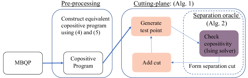
Figure 1: This figure depicts the entire solution process for solving a MBQP of the form (2.2).

In summary, we propose to solve Problem (2.2) by constructing the equivalent copositive formulation in (3.1) and applying any variant of Algorithm 1. Within Algorithm 1, the implementation of $\texttt{Oracle}(\cdot)$ is specified by Algorithm 2. This process is depicted in Figure 1. Now that we have presented our method in full, several comments are in order.

Computational complexity

While the stated complexity of the cutting-plane algorithms is applicable to any problem, it is suggestively stated in terms of the variable ${m}$. This notational overload is a deliberate choice because the dimension of the dual copositive program is equal to the total number of constraints in Problem (3.1), which is $2{m}+|B|+1=\mathcal{O}({m})$. The number of constraints can be reduced to $m+|B|+1$ using the homogenized completely positive reformulation presented in Appendix LABEL:subsec:strong_dual. While this will have no impact on the asymptotic complexity of the method, it can result in a practical reduction in runtime. If $\mathcal{T}_{Q}$ represents the oracle complexity of a particular method, the total additional overhead of converting the copositivity oracle into a separation oracle is given by $\mathcal{O}(mn^{2}\mathcal{T}_{Q})$.

Discretization size

Discretization of the copositivity check automatically introduces an approximation to the copositivity checks. The approximation fidelity is improved as the number of discretization points is increased, although it is limited by the hardware. Not only does representing a finer discretization require more qubits, but it also results in a greater skew in the coefficients of the Ising Hamiltonian. This becomes challenging since many existing hardware platforms have limited precision in their implementable couplings. In contrast, too coarse of a discretization runs the risk of missing the certificate of non-copositivity entirely. This suggests that the discretization scheme should be well-tailored to the problem at hand; Appendix LABEL:subsec:disc_cop provides guidance for choosing a discretization size based on the coefficients of the Ising Hamiltonian. A promising alternative is to circumvent discretization entirely, and apply quantum(-inspired) solvers that natively solve continuous variable box-constrained quadratic programs, such as the coherent continuous-variable machine (CCVM) recently proposed in [khosravi2022non].

Multiple cuts

Following standard convention, this work assumes that the copositivity oracle returns a single value. In contrast, in practice, many of the aforementioned Ising solvers are heuristics that involve multiple readouts. Each of these reads can be used to construct a cut, where negative, zero, and positive Ising objective values correspond to deep, neutral, and shallow cuts, respectively. Adding multiple cuts during each iteration is a possible heuristic for improving the convergence rate of the cutting-plane algorithm. While the true ground state corresponds to the deepest cut, the convergence rate guarantees stated in Table 1 hold so long as a neutral or deep cut is added at each iteration. Consequently, the proposed approach is not overly reliant on the Ising solver’s ability to identify the ground state and is resilient to heuristics. Critically, this raises the question of how to proceed if the Ising solver fails to return a certificate of non-copositivity, which will likely depend on problem specifics, such as the current outer approximation, the objective values of the samples, and the solver itself. For example, if the Ising solver returns positive but small solutions, depending on the current outer approximation, the addition of shallow cuts can still reduce the search space. On the other hand, if all non-zero solutions result in a large objective value, one could increase confidence that the test point is feasible by increasing the number of discretization points and readouts.

4 Experiments

We conducted an investigation of the proposed method on the maximum clique problem, which finds the largest complete subgraph of a graph. Given a graph, the maximum clique problem can be formulated as a completely positive program X ∈R^n ×n⟨1 1^⊤ ,   X ⟩ ⟨¯A + I ,   X ⟩ = 1 X ∈C^*_n, where $\overline{A}$ is the adjacency matrix of the graph’s complement [de2002approximation]. We note that solving the maximum clique problem is equivalent to solving the maximum independent set problem on the complement graph. The dual of (4) is the following copositive program: λ∈Rλ λ(I + ¯A) - 1 1^⊤∈C_n. This copositive program only has one variable regardless of the graph’s number of vertices or edges. Thus, we solve it with bisection, a special case of the ellipsoid algorithm, as the cutting-plane algorithm. The copositivity check’s size is determined by the number of vertices, $n$, which impacts the complexity of computing the cuts from the certificates of non-copositivity. The number of edges can be used to upper-bound the size of the maximum clique, thus determining the size of the initial feasible region; however, its effect on the complexity of checking copositivity is unclear.

(a)

(b)

(c)

Figure 2: Figure 2(a) depicts a small maximum clique example where there are edges between all vertices except $x_{4}$ and $x_{5}$. Figure 2(b) depicts the adjacency matrix of graph 2(a)’s complement, which has a single edge between vertices $x_{4}$ and $x_{5}$. Figure 2(c) depicts the solution process for the copositive cutting-plane algorithm.

4.1 QUBO Subroutine

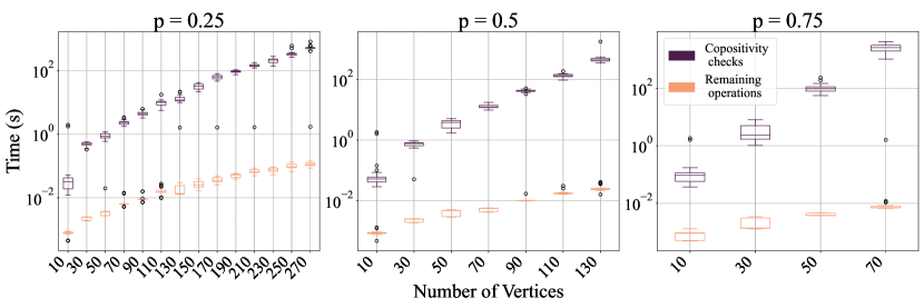
Figure 3: This figure plots the time spent on the copositivity checks versus all other operations in the proposed method. The copositivity checks grow exponentially with the number of vertices, while the other operations grow modestly.

Many hybrid algorithms are designed by replacing subroutines of existing (fully classical) algorithms with a quantum(-inspired) counterpart. An oft-neglected consideration is whether the quantum(-inspired) computer is applied to a bottleneck in the original algorithm. We contend that for a hybrid algorithm to yield significant speed-ups, the quantized subroutine should constitute the bulk of the algorithm’s complexity. In keeping with this supposition, we first evaluated whether the copositive cutting-plane algorithm shifts the complexity of the solution process onto the copositivity checks by profiling each component of the algorithm separately.

To study the scaling of each component of the proposed approach, we considered random max-clique problems with up to $10,30,\ldots,270$ vertices, where the maximum graph size varies by edge density to ensure a reasonable computation time for this experiment. For each graph size, we generated 25 random Erdős-Renyi instances with edge densities $p\in\{0.25,\,0.5,\,0.75\}$ and solved to an absolute gap of 0.9999 between upper and lower bounds (because the optimal solution is known to be integral) using the proposed copositive cutting plane algorithm. The copositivity checks were conducted by solving Anstreicher’s MILP characterization of copositivity [anstreicher2021testing] (which we found to be one of the most competitive classical formulations), using Gurobi version 9.0.3 [GurobiOptimization2020].

Figure 3 plots the time the copositive cutting plane algorithm spent on the copositivity checks versus other operations (updating the outer approximation and computing test points). The time spent on the copositivity checks scales exponentially with the number of vertices in the graph, while the time spent on other operations grows modestly. This is because Problem (4) only has one constraint regardless of the graph’s number of vertices or edges. In contrast, the size of the copositivity check is exactly equal to the number of vertices in the graph. Both the theoretical analysis and empirical results confirm that the proposed approach shifts the complexity of the copositive program onto the copositivity checks. This experiment shows that the proposed methodology is particularly effective for problems whose constraints remain constant or grow modestly with problem size.

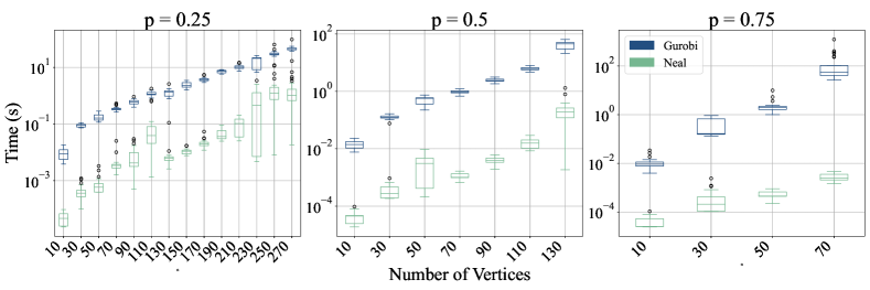
Figure 4: This figure plots the time to target to 99% confidence of the Simulated Annealing (SA) implementation in Neal (replacing the continuous feasible region, $[0,1]^{n}$, with its vertices, $\{0,1\}^{n}$) against the solution time of Gurobi for the copositivity checks. We solved each copositivity check with 100 sweeps and 1000 reads. For all densities, both methods scale exponentially with the number of vertices in the graph; however, SA is several orders of magnitude faster than Gurobi.

While undesirable for a fully classical implementation, the overwhelming complexity in the copositivity checks represents an opportunity for a quantum(-inspired) solver to beget significant speed-up. They will result from being able to execute the copositivity checks faster than the classical implementation (i.e., Anstreicher’s MILP formulation). To investigate potential speedups from using a stochastic Ising solver, we re-solved each copositivity check that yielded a certificate of non-copositivity using Simulated Annealing (SA) through the software Neal version 0.5.9, a SA sampler [DWaveNeal2021], i.e., a solver that returns samples on the solutions distribution generated by SA. Because SA is not guaranteed to find the global optima in a single annealing cycle, we define a probabilistic notion of time to target. In particular, we follow [ronnow2014defining] and define the time to target with $s$ confidence to be the number of repetitions to find the ground state at least once with probability $s$ multiplied by the time for each annealing cycle, $\texttt{T}_{\text{anneal}}$, i.e.,

(16) $$\texttt{TTT}_{s}=\texttt{T}_{\text{anneal}}\frac{\log(1-s)}{\log(1-\hat{p}_{\text{succ}})},$$

where $\hat{p}_{\text{succ}}$ is the expected value of the returned solution divided by the ground state/minimum. This results in a probability of success that interpolates between counting only solutions corresponding to the ground state and counting all certificates of non-copositivity as successes by considering the relative quality of each sample. We will also consider analogous scenarios where only ground state solutions are counted as success; we reserve the terminology “time to solution”, $\texttt{TTS}_{s}=\texttt{T}_{\text{anneal}}\frac{\log(1-s)}{\log(1-p_{\text{succ}})}$, for such cases to distinguish from the previously defined time to target. The values of $\hat{p}_{\text{succ}}$ and $p_{\text{succ}}$ is evaluated empirically over 1000 samples/reads. The time per annealing cycle, $\texttt{T}_{\text{anneal}}$, was evaluated as the total wall-clock time (for all reads) divided by the number of reads. All other Neal parameters were left as their default values.

The time to solution and time to target metrics are intended to facilitate comparison between deterministic and stochastic solvers by taking into account both the time needed to run the stochastic solver and its probability of success. It is impossible to guarantee 100% success for a stochastic solver under this formulation (mathematically, this would be equivalent to trying to compute $\texttt{TTS}_{1}$ or $\texttt{TTT}_{1}$, which are both undefined). However, computing these metrics with a high degree of certainty (e.g., $s=1-\epsilon$) is widely accepted as a tolerable, albeit imperfect, benchmark [king2015benchmarking]. In the remainder of this section, we will compare time to target metrics from SA against solution time from Gurobi, but the astute reader should keep in mind that the two solvers serve fundamentally different purposes. This comparison between the solvers is not intended to be interpreted in isolation, but rather to highlight where it might be appropriate and beneficial to substitute a heuristic Ising solver within the copositive cutting-plane framework.

For each copositivity check solved, we considered discretizations corresponding to ${\min_{\hat{z}\in\{0,\,1\}^{n}}\hat{z}^{\top}M\hat{z}}$ (i.e., no additional problem discretization). We solved each copositivity check with 100 sweeps and 1000 reads. Figure 4 plots the time to target with 99% confidence from Neal against the solution time from Gurobi. We see that for all graph sizes, Neal can consistently find certificates of non-copositivity in orders of magnitude less time than Gurobi. Notably, Neal and Gurobi demonstrate similar scaling with respect to the number of vertices.

Unlike SA, which operates without reference to rigorous optimality bounds, Gurobi’s solution process tracks both upper and lower bounds on the objective value and terminates only when they reach user-specified stopping conditions. To evaluate whether the optimal objective is found early in the solution process and time is spent closing the upper bounds, we plotted Gurobi’s lower and upper bounds progress against time together with $\texttt{TTT}_{0.99}$ and $\texttt{TTT}_{0.999}$ in Figure 5 for instances with density $p=0.25$. Analogous plots for other densities are included in the Appendix. For each graph size, we plotted the instances where the ratio between Gurobi’s solution time and $\texttt{TTT}_{0.99}$ is the greatest (top row) and least (bottom row)–all instances were run with 100 sweeps. For each instance, we plot Gurobi’s upper bound (purple, solid) and best objective found (red, dashed), and Neal $\texttt{TTT}_{0.99}$ (light teal, dashed), and $\texttt{TTT}_{0.999}$ (dark teal, dash-dot) (colored figures are available online). We found that in most instances, Neal reaches the time to target with 99.9% confidence before Gurobi even returns a callback (i.e., when the dark teal, dash-dot line does not intersect either of the purple-solid or red-dashed lines); this is likely due to an initial pre-processing step. Pre-processing is a necessary overhead for Gurobi’s intended purpose of proving optimality, thus hampering its relative performance on smaller or easier problems. Critically, in the proposed approach, optimality guarantees are only necessary for cases where the test point is copositive, while the algorithm can make progress with any certificate of non-copositivity, even if it is not globally optimal. This suggests that heuristics (e.g., Ising solvers) and complete methods (e.g., Gurobi) could play complementary roles within the same copositive cutting-plane algorithm. For example, for some test points, one may avoid the overhead of Gurobi altogether if the Ising solver quickly returns a certificate of non-copositivity. On the other hand, if the Ising solver fails to generate such a certificate, one may rely on Gurobi for proving that the test point is copositive.

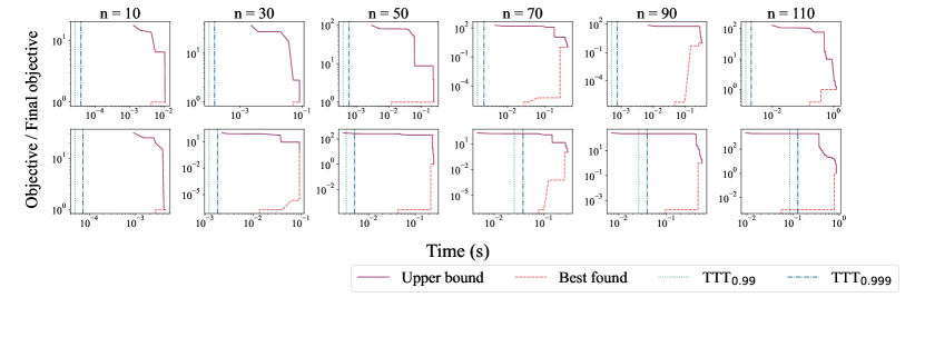
Figure 5: This figure depicts sample trajectories of Gurobi’s upper and lower bounds against $\texttt{TTT}_{0.99}$ and $\texttt{TTT}_{0.999}$ for edge density $p=0.25$. For each graph size, the top row represents the instance where the ratio between Gurobi’s solution time and $\texttt{TTT}_{0.99}$ is the greatest, and the bottom row represents the instance where the ratio is the smallest–all instances were run with 100 sweeps. In most instances, Neal reaches the $\texttt{TTT}_{0.999}$ confidence before Gurobi even returns a callback.

4.2 Overall Cutting-Plane Algorithm

Next, we compared the copositive cutting-plane algorithm with the SA implementation in Neal as the Ising solver against solving a mixed-integer linear program (MILP) formulation of maximum-clique directly with Gurobi. Gurobi’s solution time was evaluated on the following MILP formulation of maximum clique: x ∈{0, 1}^n1^⊤x x_i + x_j ≤1,  ∀(i, j) ∈