Elastic membranes spanning deformable boundaries

F.  Ballarin1   $-$  G. Bevilacqua2   $-$   L. Lussardi2   $-$  A.  Marzocchi1

1 Dipartimento di Matematica e Fisica “N. Tartaglia
francesco.ballarin@unicatt.itgiulia.bevilacqua@polito.it luca.lussardi@polito.it alfredo.marzocchi@unicatt.it
Università Cattolica del Sacro Cuore
via della Garzetta 48
I-25133 Brescia Italy
2 Dipartimento di Scienze Matematiche “G.L. Lagrange
Politecnico di Torino
c.so Duca degli Abruzzi 24
I-10129 Torino Italy.
Abstract

We perform a variational analysis of an elastic membrane spanning a curve which may sustain bending and torsion. First, we deal with parametrized curves and linear elastic membranes proving the existence of equilibria and finding first-order necessary conditions for minimizers computing the first variation. Second, we study a more general case, both for the boundary curve and the membrane, using the framed curve approach. The infinite dimensional version of the Lagrange multipliers’ method is applied to get the first-order necessary conditions. Finally, a numerical approach is presented and employed in several numerical test cases.

Keywords: critical points, elastic membranes, elastic curves, finite element method

MSC 2020: 49J45, 49Q05, 74K15, 74B20, 74S05

1 Introduction

Minimal surfaces and elastic membranes are classical topics very well investigated from the variational point of view: there exists a huge literature on the existence of solutions, while the study of critical surfaces received less attention. The interest in the minimization of the area functional dates back to Lagrange [34] and Plateau [44], since they formulated, separately and from a mathematical and physical point of view respectively, the famous Plateau problem. The first rigorous solution has been presented around 1930 by Douglas and Radó [24, 45] where the area functional is replaced by the Dirichlet one in conformal coordinates. From such a result, in the last century, many mathematicians looked for a more general and weaker definition of surface, for instance integral currents, finite perimeter sets and Almgren minimal sets (see for instance [27, 2, 47] and a complete review [21] with references therein).

Recently, using a result by Lytchak and Wenger [39], Creutz [19] proved the existence of a minimizer for the classical area functional for disc-type surfaces spanning a curve with possible self-intersections. Precisely, let $\boldsymbol{\gamma}$ be a curve in $\mathbb{R}^{3}$ (not necessarily simple), $D$ be the unit disc in $\mathbb{R}^{2}$ and $\boldsymbol{X}\colon D\to\mathbb{R}^{3}$ be an immersion of the disc in $\mathbb{R}^{3}$. In [19], Creutz proved that the area functional

$\displaystyle\mathcal{A}[\boldsymbol{X}]:=\int_{D}\left\lvert\boldsymbol{X}_{u}\wedge\boldsymbol{X}_{v}\right\rvert\,dudv,$

is minimized among all $\boldsymbol{X}\in W^{1,2}(D;\mathbb{R}^{3})$ such that the trace of $\boldsymbol{X}$ is a reparametrization of the boundary curve $\boldsymbol{\gamma}$. The main difficulty of such a result is to get compactness, since the boundary curve may not be a Jordan type: in the Douglas-Radó approach the fact that the boundary curve is a Jordan one is crucial.

If the boundary curve is assumed to be elastic to model, for instance, the absorption of proteins through biological membranes, few results are known, both in the existence of solutions and in the derivation of Euler-Lagrange equations. This happens due to a competition between the surface energy and the elasticity of the boundary curve.

In [8], Bernatzki and Ye considered elastic curves spanned by disc-type surfaces and they proved the existence of an area minimizing current. However, to avoid self-intersections, they were forced to introduce a technical condition on the surface tension coefficient (see Hypothesis 2.1 in [8]). Next, Giomi and Mahadevan studied the stability of critical points of the elastic Plateau problem using asymptotic techniques and provided numerical simulations [30]. We also mention [42] where minimal surfaces spanning an elastic ribbon described through the Darboux framework are considered.

A related problem considers an elastic rod instead of a curve. In this direction there are some results on the existence of minima of the energy under physical constraints [14, 15, 31, 9, 10, 11], whereas the derivation of the Euler-Lagrange equations for the critical points seems to be hard for two reasons. On one hand the presence of constraints on the rod makes difficult to work with the corresponding variations. On the other hand, the regularity of the contact set between rod and surface is not yet known even for a fixed simple boundary [22].

For all these reasons, we focus our attention on elastic boundary curves instead of rods. To allow for self-intersections, which are physically evident, in [13] we derived the existence of minimizers of a functional of the following type

$$\mathcal{F}[\boldsymbol{\gamma}]=\int_{\boldsymbol{\gamma}}f(\kappa,\tau)\,d\boldsymbol{\gamma},$$

where $\kappa$ and $\tau$ are suitable notions of signed curvature and torsion of the curve $\boldsymbol{\gamma}$ which may not be simple. Moreover, in the same paper, we also investigated the first-order necessary conditions for minimizers by means of an application of the infinite version of the Lagrange multipliers’ method. This was the first result where the elastic curve is less regular, at most $C^{1}$, and the energy density penalizes not only the curvature but also the torsion (see for classical theory of elasticae [20, 28] and references therein)

A natural problem arising from the above considerations is to study the following functional

$$\mathcal{G}[\boldsymbol{\gamma},\boldsymbol{X}]=\int_{\boldsymbol{\gamma}}f(\kappa,\tau)\,d\boldsymbol{\gamma}+\int_{D}\left\lvert\boldsymbol{X}_{u}\wedge\boldsymbol{X}_{v}\right\rvert\,dudv,$$

where the trace of $\boldsymbol{X}$ is a reparametrization of $\boldsymbol{\gamma}$. Since we look for physical minimizers of $\mathcal{G}$, in particular we expect to deal with Plateau’s type singularities, we need to use a Geometric Measure Theory framework and this will be the content of a forthcoming paper [12].

On the contrary, willing to remain in a Sobolev setting, we look in this paper to the same model but for elastic membranes, that is, we consider the energy functional

$$\mathcal{E}[\boldsymbol{\gamma},\boldsymbol{X}]=\int_{\boldsymbol{\gamma}}f(\kappa,\tau)\,d\boldsymbol{\gamma}+\int_{D}\Psi(\nabla\boldsymbol{X})\,dudv,$$

where both $f$ and $\Psi$ have superlinear growth. This is the suitable setting to derive the first-order necessary conditions for minimizers. Precisely, we study minimizers among all $\boldsymbol{X}$ with trace pointwise equal to $\boldsymbol{\gamma}$: this choice of spanning condition will be crucial to derive first-order necessary conditions for minimizers.

The choice of modeling elastic membranes though the deformation gradient $\nabla\boldsymbol{X}\in M^{3\times 2}$ is not new but it has been widely studied both from a physical and a mathematical points of view. For instance, we mention tension field theory, which has been introduced to study fundamental stress-strain relations for isotropic elastic membranes [43, 7], and the rigorous derivation of its form and properties obtained around 1990 by Le Dret and Raoult though a $\Gamma$-convergence result [35, 36, 37].

In the following sections, we are going to present the main results obtained throughout the paper and the adopted techniques together with the encountered difficulties.

1.1 Main results

In this work, we are going to consider functionals of the form

$$\mathcal{E}[\boldsymbol{\gamma},\boldsymbol{X}]=\int_{\boldsymbol{\gamma}}f(\kappa,\tau)\,d\boldsymbol{\gamma}+\int_{D}\Psi(\nabla\boldsymbol{X})\,dudv,$$ (1.1)

where $\boldsymbol{\gamma}$ is an elastic curve whose behaviour depends on the curvature $\kappa$ and the torsion $\tau$, while $\boldsymbol{X}:D\to\mathbb{R}^{3}$ is the immersion of the disc $D$ into $\mathbb{R}^{3}$ and $\Psi$ is an elastic energy density depending only on the gradient, which is a quite common approach in a continuum mechanics problem.

A first way to deal with the line integral is to use parametrized curves. With this approach, we can treat the Euler-Bernoulli elastica for $\boldsymbol{\gamma}$ and linearly elastic membrane. More precisely, we consider the following functional

$$\mathcal{E}_{p}[\boldsymbol{r},\boldsymbol{X}]=\int_{0}^{2\pi}\left\lvert\boldsymbol{r}^{\prime\prime}(\vartheta)\right\rvert^{2}\,d\vartheta+\frac{\mu}{2}\int_{D}\textgoth{C}\nabla\boldsymbol{X}(u,v):\nabla\boldsymbol{X}(u,v)\,dudv.$$ (1.2)

Here, $\boldsymbol{r}\in W^{2,2}((0,2\pi);\mathbb{R}^{3})$ is a $C^{1}$-periodic curve clamped at a fixed point and parametrized by arc-length. Moreover, $\mu>0$ is the shear modulus, $\boldsymbol{X}\in W^{1,2}(D;\mathbb{R}^{3})$ is the disc-type parametrization of the membrane, $\textgoth{C}$ is the linear elasticity tensor which should depend on the point $\boldsymbol{p}\in D$. In addition, we require that

$${\rm Tr}\,\boldsymbol{X}(\cos\vartheta,\sin\vartheta)=\boldsymbol{r}(\vartheta),\quad\text{a.e.\,$\vartheta\in(0,2\pi)$},$$

where ${\rm Tr}$ is the trace operator on the boundary. In this setting we are able to prove:

Theorem 1.1.

(Parametrized curve approach, see Theorems 2.5 and 2.8)
The functional $\mathcal{E}_{p}$ admits minimizers and they satisfy the following first-order necessary conditions

$$\left\{\begin{aligned} &{\rm div}\left(\textgoth{C}\nabla\boldsymbol{X}\right)(u,v)=0,&&&(u,v)\in D\\ &\left[2\boldsymbol{r}^{(iv)}(\vartheta)+\mu\,\textgoth C\nabla\boldsymbol{X}(\cos\vartheta,\sin\vartheta)\boldsymbol{\nu}(\vartheta)\right]_{\perp,\boldsymbol{r}}=0,&&&\hbox{a.e. }\vartheta\in(0,2\pi)\end{aligned}\right.$$ (1.3)

where $\boldsymbol{\nu}$ is the outer normal of the disc $D$ and $\boldsymbol{v}_{\perp,\boldsymbol{r}}$ denotes the orthogonal component of $\boldsymbol{v}$ on $\boldsymbol{r}^{\prime}$.

In order to deal with more general elastic energies for the curve, which for instance involve also the torsion, we use the framed curve approach. In particular, this allows to consider also non-linear elastic energy for the membrane. We introduce a moving orthonormal frame $\left\{\boldsymbol{t},\boldsymbol{n},\boldsymbol{b}\right\}\in W^{1,p}((0,2\pi);SO(3))$ with $p>1$ which generates a curve $\boldsymbol{r}$ by integration and we define the energy in terms of the frame as

$$\mathcal{E}_{f}\left[\left(\boldsymbol{t}|\boldsymbol{n}|\boldsymbol{b}\right),\boldsymbol{X}\right]=\int_{0}^{2\pi}f(\kappa(\vartheta),\tau(\vartheta))\,d\vartheta+\frac{\mu}{2}\int_{D}\Psi(\nabla\boldsymbol{X})\,dudv,$$ (1.4)

where $\kappa=\boldsymbol{t}^{\prime}\cdot\boldsymbol{n}$ and $\tau=\boldsymbol{n}^{\prime}\cdot\boldsymbol{b}$ play the role of weak signed curvature and weak torsion respectively. Here, as in the previous case the pointwise trace constraint holds, i.e.

$${\rm Tr}\,\boldsymbol{X}(\cos\vartheta,\sin\vartheta)=\boldsymbol{r}(\vartheta),\quad\text{a.e.\,$\vartheta\in(0,2\pi)$}.$$

In this framework, we can prove the following result

Theorem 1.2.

(Framed curve approach, see Theorems 3.3 and 3.5)
Assume $f$ is a convex function, $f(a,b)\geq c_{1}\left\lvert a\right\rvert^{p}+c_{2}\left\lvert b\right\rvert^{p}+c_{3}$ for some $c_{1},c_{2}>0$ and $c_{3}\in\mathbb{R}$ and $p>1$. Moreover, assume $\Psi$ is continuous, quasiconvex (see Definition 3.2) and it satisfies $c_{4}\left\lvert\mathsf{A}\right\rvert^{q}\leq\Psi(\mathsf{A})\leq c_{5}\left\lvert\mathsf{A}\right\rvert^{q}$ for some $c_{4},c_{5}>0$ and $q>1$. Then $\mathcal{E}_{f}$ has a minimizer. Moreover if

  • (a)

    $f$ is of class of $C^{1}$ and that there is $\alpha>0$ such that

    |fa(a,b)|α(1+|a|p1+|b|p1),subscript𝑓𝑎𝑎𝑏𝛼1superscript𝑎𝑝1superscript𝑏𝑝1\displaystyle\left\lvert f_{a}(a,b)\right\rvert\leq\alpha\left(1+\left\lvert a\right\rvert^{p-1}+\left\lvert b\right\rvert^{p-1}\right), |fb(a,b)|α(1+|a|p1+|b|p1),subscript𝑓𝑏𝑎𝑏𝛼1superscript𝑎𝑝1superscript𝑏𝑝1\displaystyle\left\lvert f_{b}(a,b)\right\rvert\leq\alpha\left(1+\left\lvert a\right\rvert^{p-1}+\left\lvert b\right\rvert^{p-1}\right),

    for all $a,b\in\mathbb{R}$

  • (b)

    there is $\beta>0$ such that

    |DΨ(𝖠)|β(1+|𝖠|2)DΨ𝖠𝛽1superscript𝖠2\left\lvert{\rm D}\Psi(\mathsf{A})\right\rvert\leq\beta\left(1+\left\lvert\mathsf{A}\right\rvert^{2}\right)

    for all $\mathsf{A}\in M^{3\times 2}$,

then for each minimizer there exist $\omega\in L^{p}((0,2\pi))$, $\boldsymbol{\chi}\in L^{2}((0,2\pi);\mathbb{R}^{3})$ and $\boldsymbol{\lambda}\in\mathbb{R}^{3}$ such that the following first-order necessary conditions hold a.e. $(u,v)\in D$ and $\vartheta\in[0,2\pi]$

$$\left\{\begin{aligned} &\operatorname{div}\,\left({\rm D}\Psi(\nabla\boldsymbol{X})\right)=0,&&\hbox{on }D,\\ &-f_{a}^{\prime}-\omega\tau-\left[\int_{0}^{\vartheta}\boldsymbol{\chi}(\xi)\,d\xi\right]\cdot\boldsymbol{n}=\boldsymbol{\lambda}\cdot\boldsymbol{n},&&\hbox{on }\partial D,\\ &-f_{a}\tau+\omega^{\prime}+f_{b}\kappa-\left[\int_{0}^{\vartheta}\boldsymbol{\chi}(\xi)\,d\xi\right]\cdot\boldsymbol{b}=\boldsymbol{\lambda}\cdot\boldsymbol{b},&&\hbox{on }\partial D,\\ &\frac{\mu}{2}\left({\rm D}\Psi(\nabla\boldsymbol{X})\right)\boldsymbol{\nu}=\boldsymbol{\chi},&&\hbox{on }\partial D,\\ &\omega\kappa-f^{\prime}_{b}=0,&&\hbox{on }\partial D.\end{aligned}\right.$$

We are finally able to eliminate all the Lagrange multipliers for smooth critical points whenever $\kappa\neq 0$, see Theorem 3.7

Finally, to deal with the requirements of numerical simulations, we introduce the following functional

$$\mathcal{E}_{n}[\boldsymbol{X}]=\int_{\partial D}\left\lvert\partial_{\vartheta\vartheta}\boldsymbol{X}\right\rvert^{2}\,d\vartheta+\frac{\mu}{2}\int_{D}\textgoth{C}\nabla\boldsymbol{X}(u,v):\nabla\boldsymbol{X}(u,v)\,dudv,$$ (1.5)

where $\boldsymbol{X}\in W^{3,2}(D;\mathbb{R}^{3})$ is the disc parametrization of the elastic membrane, $\partial_{\vartheta}$ is the tangential directional derivative on the boundary of the disk $\partial D$, and $\textgoth{C}$ is the linear elasticity tensor which may depend on the point $\boldsymbol{p}\in D$. We identify the curve $\boldsymbol{r}$ with the trace of the map $\boldsymbol{X}$, namely ${\rm Tr}\,\boldsymbol{X}\in W^{\frac{5}{2},2}(\partial D;\mathbb{R}^{3})$. Furthermore, we require

$$\left|\partial_{\vartheta}\boldsymbol{X}\right|=1,\quad\text{on}\quad\partial D,\qquad\text{and}\qquad\int_{D}\boldsymbol{X}\;dudv=\boldsymbol{0},$$ (1.6)

i.e., we are imposing the length preserving constraint and avoiding rigid motions. However, in practice for technical convenience the first constraint is imposed weakly by means of the following auxiliary functional

$$\widetilde{\mathcal{E}}_{n}[\boldsymbol{X},\ell]=\int_{\partial D}\left\lvert\partial_{\vartheta\vartheta}\boldsymbol{X}\right\rvert^{2}\,d\vartheta+\frac{\mu}{2}\int_{D}\textgoth{C}\nabla\boldsymbol{X}(u,v):\nabla\boldsymbol{X}(u,v)\,dudv+\int_{\partial D}\ell\;\left[\left|\partial_{\vartheta}\boldsymbol{X}\right|^{2}-1\right]d\vartheta,$$ (1.7)

where $\ell\in W^{\frac{1}{2},2}(\partial D;\mathbb{R})$ is an infinite-dimensional Lagrange multiplier. In this setting, we are able to prove

Theorem 1.3.

(Numerical approach, see Theorem 4.1)
Any minimizers of $\widetilde{\mathcal{E}}_{n}[\boldsymbol{X},\ell]$ satisfy the following first-order necessary conditions:

$$\left\{\begin{aligned} &\mu\int_{D}\textgoth{C}\nabla\boldsymbol{X}:\nabla\boldsymbol{V}\,dudv+2\int_{\partial D}\partial_{\vartheta\vartheta}\boldsymbol{V}\cdot\partial_{\vartheta\vartheta}\boldsymbol{X}\,d\vartheta+2\int_{\partial D}\ell\;\partial_{\vartheta}\boldsymbol{V}\cdot\partial_{\vartheta}\boldsymbol{X}\;d\vartheta=0,\\ &\int_{\partial D}m\;\left[\left|\partial_{\vartheta}\boldsymbol{X}\right|^{2}-1\right]d\vartheta=0,\end{aligned}\right.$$ (1.8)

for every $(\boldsymbol{V},m)\in C^{\infty}(\overline{D};\mathbb{R}^{3})\times C^{\infty}(\overline{\partial D};\mathbb{R})$ such that $\int_{D}\boldsymbol{V}\;dudv=\boldsymbol{0}$.

Such numerical approach will then be employed in several numerical test cases which will show a typical behavior of the Dirichlet energy functional, i.e. the possibility of planar or non-planar self-intersections [40].

1.2 Main issues and outline of the paper

Different from the area functional, in this work, we introduce an elastic membrane to model the stretch contribution of the surface, with an energy density function $\Psi$ depending on the deformation gradient $\nabla\boldsymbol{X}$, and being quasiconvex.

The functional $\mathcal{E}$ depends on two variables, i.e. the elastic curve $\boldsymbol{\gamma}$ and the immersed map $\boldsymbol{X}$ from the unit disc to $\mathbb{R}^{3}$. Nevertheless, it is not convenient to rewrite it as a functional depending only on $\boldsymbol{X}$

$$\mathcal{E}[\boldsymbol{X}]=\int_{\partial D}f(\kappa,\tau)\,d\mathcal{H}^{1}+\int_{D}\Psi(\nabla\boldsymbol{X})\,dudv,$$

like in [30, 42]: the integral over the curve $\boldsymbol{\gamma}$ has to be rewritten as a function of the ${\rm Tr}\,\boldsymbol{X}$ and this leads to a much more complicated expression of the curvature since ${\rm Tr}\,\boldsymbol{X}$ may not be parametrized by arc-length. Moreover, for the same reason, we would need to require higher regularity on $\boldsymbol{X}$, loosing compactness since only its $H^{1}$ norm can be bounded along minimizing sequences. Nevertheless, in the numerical section we just consider the membrane map $\boldsymbol{X}$ as independent variable, since reducing the complexity of the problem has beneficial effects both in terms of implementation and convergence of the nonlinear iterations.

Concerning the constraint to link the membrane $\boldsymbol{X}$ with the curve $\boldsymbol{\gamma}$, differently from the Douglas-Radó approach, where ${\rm Tr}\,\boldsymbol{X}$ is a reparametrization of $\boldsymbol{\gamma}$, we impose the pointwise constraint

$${\rm Tr}\,\boldsymbol{X}(\cos\vartheta,\sin\vartheta)=\boldsymbol{\gamma}(\vartheta),\qquad\vartheta\in[0,2\pi].$$

Indeed, using the trace condition as in Douglas-Radó, we cannot prove the existence of minimizers since their method works only for a Jordan fixed curve, while our curves are elastic allowing for self-intersections. On the other hand, our pointwise constraint is the right one to apply the Direct Methods of the Calculus of Variations since the Trace Theorem holds here. In addition, this pointwise constraint strongly complicates the derivation of the Euler-Lagrange equations, especially in the first part of the paper, where we adopt the parametrized approach for the curve. Indeed, it is hard to find variations of the surface which fulfill the trace constraint. Hence, we introduce an auxiliary energy functional where the trace constraint is imposed trough a Lagrange multiplier $\lambda$ and we derive the Euler-Lagrange equations for the “free" energy, namely the one with no constraints. Then, we prove that when $\lambda\to+\infty$, the minimizers converge to the ones of the original functional $\mathcal{E}$ defined in Eq. (1.1).

In order to propose a discretization of the minimization of the following functional,

$$\mathcal{E}[\boldsymbol{\gamma},\boldsymbol{X}]=\int_{\boldsymbol{\gamma}}\kappa^{2}\,d\boldsymbol{\gamma}+\int_{D}\textgoth{C}\nabla\boldsymbol{X}:\nabla\boldsymbol{X}\,dudv,$$ (1.9)

we deem convenient to identify the elastic curve $\boldsymbol{\gamma}$ with the trace of the parametrized map $\boldsymbol{X}$. On one hand, this choice is computationally convenient since it allows to consider a single unknown $\boldsymbol{X}$, thus satisfying by construction the identification constraints between $\boldsymbol{X}$ and $\boldsymbol{\gamma}$. On the other hand, we now need to increase the necessary regularity $\boldsymbol{X}\in W^{3,2}(D;\mathbb{R}^{3})$ for the first integral to be well-defined, namely to guarantee that ${\rm Tr}\,\boldsymbol{X}\in W^{\frac{5}{2},2}(\partial D;\mathbb{R}^{3})$. The corresponding discretization by a finite element method would thus require a $C^{2}$ continuity across cells, which is different from the standard $C^{0}$ requirement of Lagrange finite elements. Since the definition of finite elements with such an higher order continuity is challenging and not readily available on commonly used open-source implementations, in Section 4 we will exploit an alternative way to reformulate the discrete problem.

Furthermore, another important aspect of the numerical approach is how to impose the length preserving constraint, since a pointwise formulation is ill-suited in the application of a finite element method. Hence, by introducing an additional unknown, we will replace such constraint by an integral formulation through an infinite-dimensional Lagrange multiplier defined only on the boundary of the disc. The additional unknown, being defined only on the boundary, only marginally increases the overall computational cost.

We finally remark that the use of framed curves allows to consider a more general class of functionals, differently from the parametrized approach where just the curvature can be penalized and elastic energy densities for the membrane are linear, for which the Lagrange multipliers’ method successfully applies.

The paper is organized as follows: in Section 2 we prove the existence of minimizers and we derive the Euler-Lagrange equations for the parametrized curve approach; in Section 3, we overcome the limitations of the previous result modeling the curve as a framed curve proving the existence of minimizers, getting the first-order necessary conditions and proving the equivalence of the equations for critical points in the specific case studied in Section 2. Afterwards, in Section 4 we introduce an ad hoc method to be employed in the numerical simulations testing it in some cases in Section 5. Finally, in Section 6 we conclude with some comments and remarks.

2 The parametrized curve approach

2.1 Setting of the problem

We assume that the boundary elastic curve is closed it is clamped at a fixed point $\boldsymbol{x}_{0}$ and it has fixed length. More precisely, fix $\boldsymbol{x}_{0}\in\mathbb{R}^{3}$ and let $\boldsymbol{r}\in W^{2,2}((0,2\pi);\mathbb{R}^{3})$ be such that:

$\displaystyle\boldsymbol{r}(0)=\boldsymbol{r}(2\pi)=\boldsymbol{x}_{0},$ (2.1)
$\displaystyle\boldsymbol{r}^{\prime}(0)=\boldsymbol{r}^{\prime}(2\pi),$ (2.2)
$\displaystyle\left|\boldsymbol{r}^{\prime}(\vartheta)\right|=1,\quad\forall\vartheta\in[0,2\pi].$ (2.3)

Notice that conditions Eqs. (2.1) and (2.2) make sense since $\boldsymbol{r}\in C^{1}([0,2\pi];\mathbb{R}^{3})$. The elastic membrane is assumed to be a smooth disc-type parametrization $\boldsymbol{X}\in W^{1,2}(D;\mathbb{R}^{3})$, where $D:=\{(u,v)\in\mathbb{R}^{2}:u^{2}+v^{2}<1\}$. Moreover, the following constraint has to be satisfied by $\boldsymbol{r}$ and $\boldsymbol{X}$

$\displaystyle{\rm Tr}\,\boldsymbol{X}(\cos\vartheta,\sin\vartheta)=\boldsymbol{r}(\vartheta),\quad\text{a.e.\,$\vartheta\in(0,2\pi)$}.$ (2.4)

Notice that the quantity ${\rm Tr}\,\boldsymbol{X}(\cos\vartheta,\sin\vartheta)$ is well defined even if ${\rm Tr}\,\boldsymbol{X}\in W^{\frac{1}{2},2}(\partial D;\mathbb{R}^{3})$, since the map $\vartheta\mapsto(\cos\vartheta,\sin\vartheta)$ is a bijection as a map $[0,2\pi)\to\partial D$. Let

$$\mathcal{W}_{p}=W^{2,2}((0,2\pi);\mathbb{R}^{3})\times W^{1,2}(D;\mathbb{R}^{3}),$$

where the subscript $p$ refers to the parametric approach adopted here. On $\mathcal{W}_{p}$ we consider the product weak topology, namely $(\boldsymbol{r}_{h},\boldsymbol{X}_{h})\rightharpoonup(\boldsymbol{r},\boldsymbol{X})$ means that $\boldsymbol{r}_{h}\rightharpoonup\boldsymbol{r}$ in $W^{2,2}((0,2\pi);\mathbb{R}^{3})$ and $\boldsymbol{X}_{h}\rightharpoonup\boldsymbol{X}$ in $W^{1,2}(D;\mathbb{R}^{3})$. The set of constraints is given by

𝒞p={(𝒓,𝑿)𝒲p:(2.1) - (2.2) - (2.3) - (2.4) hold true}.subscript𝒞𝑝conditional-set𝒓𝑿subscript𝒲𝑝(2.1) - (2.2) - (2.3) - (2.4) hold true\mathcal{C}_{p}=\left\{(\boldsymbol{r},\boldsymbol{X})\in\mathcal{W}_{p}:\text{\eqref{eq:r_0} - \eqref{eq:rprimo0} - \eqref{eq:velocita_1} - \eqref{eq:traccia} hold true}\right\}.

Now, we introduce the energy functional. Let $\mathcal{E}_{p}\colon\mathcal{C}_{p}\to[0,+\infty)$ be given by

$$\mathcal{E}_{p}[\boldsymbol{r},\boldsymbol{X}]=\int_{0}^{2\pi}\left\lvert\boldsymbol{r}^{\prime\prime}(\vartheta)\right\rvert^{2}\,d\vartheta+\frac{\mu}{2}\int_{D}\textgoth{C}\nabla\boldsymbol{X}(u,v):\nabla\boldsymbol{X}(u,v)\,dudv$$ (2.5)

where $\mu>0$ is the shear modulus, measuring the softness of the membrane, and $\forall\boldsymbol{p}\in D$, $\textgoth{C}(\boldsymbol{p})\colon M^{3\times 2}\to M^{3\times 2}$ is linear and continuous with

$$\alpha\left\lvert\zeta\right\rvert^{2}\leq\textgoth{C}\zeta:\zeta\leq\beta\left(1+\left\lvert\zeta\right\rvert^{2}\right),\qquad\forall\,\zeta\in M^{3x2},$$ (2.6)

for some $\alpha,\beta>0$.

Our goal is to minimize $\mathcal{E}_{p}$ and to find first-order necessary conditions for suitable minimizers.

2.2 Some preliminary lemmas

In this subsection, we are going to prove closure of the constraint set $\mathcal{C}_{p}$ and the compactness of sequences of equi-boundeness energy.

Lemma 2.1.

Let $(\boldsymbol{r}_{h})$ be a sequence in $W^{2,2}((0,2\pi);\mathbb{R}^{3})$ satisfying conditions (2.1) - (2.2) - (2.3), and let $(\boldsymbol{X}_{h})$ be a sequence in $W^{1,2}(D;\mathbb{R}^{3})$. Assume that

$$\int_{0}^{2\pi}\left\lvert\boldsymbol{r}_{h}^{\prime\prime}(\vartheta)\right\rvert^{2}\,d\vartheta+\frac{\mu}{2}\int_{D}\textgoth{C}\nabla\boldsymbol{X}_{h}(u,v):\nabla\boldsymbol{X}_{h}(u,v)\,dudv\leq c$$

for some $c\geq 0$. Then there exists $(\boldsymbol{r},\boldsymbol{X})\in\mathcal{W}_{p}$ such that, up to a subsequence, $(\boldsymbol{r}_{h},\boldsymbol{X}_{h})\stackrel{{\scriptstyle}}{{\rightharpoonup}}(\boldsymbol{r},\boldsymbol{X})$ weakly in $\mathcal{W}_{p}$. Moreover, $\boldsymbol{r}$ satisfies conditions (2.1) - (2.2) - (2.3).

Proof.

First of all we have $\left\lVert\boldsymbol{r}^{\prime\prime}_{h}\right\rVert_{L^{2}}\leq c$. Eq. (2.3) implies that $\|\boldsymbol{r}^{\prime}_{h}\|_{L^{2}}=\sqrt{2\pi}$. Finally, since $\boldsymbol{r}_{h}$ is clamped at $\boldsymbol{x}_{0}$ we get

$$\boldsymbol{r}_{h}(\vartheta)=\boldsymbol{x}_{0}+\int_{0}^{\vartheta}\boldsymbol{r}_{h}^{\prime}(s)\,ds$$

from which $\|\boldsymbol{r}_{h}\|_{L^{2}}\leq c^{\prime}$ for some other positive constant $c^{\prime}$. As a consequence, $\left\lVert\boldsymbol{r}_{h}\right\rVert_{W^{2,2}}$ is bounded, and then, up to a subsequence, $\boldsymbol{r}_{h}\rightharpoonup\boldsymbol{r}$ in $W^{2,2}((0,2\pi);\mathbb{R}^{3})$ for some $\boldsymbol{r}\in W^{2,2}((0,2\pi);\mathbb{R}^{3})$. By Sobolev embeddings we get $\boldsymbol{r}_{h}\to\boldsymbol{r}$ strongly in $C^{1}$. As a consequence, conditions (2.1) - (2.2) - (2.3) pass easily to the limit. Now, using the coercivity condition (2.6) we easily deduce that $\|\nabla\boldsymbol{X}_{h}\|_{L^{2}}$ is bounded. Now, we prove that also $\|\boldsymbol{X}_{h}\|_{L^{2}}$ is bounded. For any $(u,v)\in\partial D$ we let $\tilde{\boldsymbol{r}}_{h}(u,v)=\boldsymbol{r}_{h}(\vartheta)$ where $\vartheta\in[0,2\pi)$ is the unique angle such that $u=\cos\vartheta$ and $v=\sin\vartheta$. Take $\boldsymbol{Y}_{h}=\text{Ext}\,\tilde{\boldsymbol{r}}_{h}$ and let $\boldsymbol{Z}_{h}=\boldsymbol{X}_{h}-\boldsymbol{Y}_{h}$. By construction $\boldsymbol{Z}_{h}\in W^{1,2}_{0}(D;\mathbb{R}^{3})$. Combining the triangle inequality with the Poincaré inequality and the extension embedding Ext we get

$\displaystyle\|\boldsymbol{X}_{h}\|_{L^{2}}$ $\displaystyle\leq\|\boldsymbol{Z}_{h}\|_{L^{2}}+\|\boldsymbol{Y}_{h}\|_{L^{2}}$
$\displaystyle\leq c_{1}\|\boldsymbol{\nabla}Z_{h}\|_{L^{2}}+\|\boldsymbol{Y}_{h}\|_{L^{2}}$
$\displaystyle\leq c_{1}\|\nabla\boldsymbol{X}_{h}\|_{L^{2}}+c_{2}\|\boldsymbol{Y}_{h}\|_{W^{1,2}}$
$\displaystyle\leq c_{1}\|\nabla\boldsymbol{X}_{h}\|_{L^{2}}+c_{3}\|\boldsymbol{r}_{h}\|_{W^{2,2}}$
$\displaystyle\leq c_{4}.$

As a consequence, up to a subsequence, $\boldsymbol{X}_{h}\rightharpoonup\boldsymbol{X}$ in $W^{1,2}(D;\mathbb{R}^{3})$ for some $\boldsymbol{X}\in W^{1,2}(D;\mathbb{R}^{3})$, and this concludes the proof. ∎

Lemma 2.2.

$\mathcal{C}_{p}$ is weakly closed in $\mathcal{W}_{p}$.

Proof.

Let $(\boldsymbol{r}_{h},\boldsymbol{X}_{h})$ be a sequence in $\mathcal{C}_{p}$ with $(\boldsymbol{r}_{h},\boldsymbol{X}_{h})\rightharpoonup(\boldsymbol{r},\boldsymbol{X})$ for some $(\boldsymbol{r},\boldsymbol{X})\in\mathcal{W}_{p}$. By Lemma 2.1 we can say that $\boldsymbol{r}$ satisfies conditions (2.1) - (2.2) - (2.3). We prove now that $(\boldsymbol{r},\boldsymbol{X})$ satisfies also condition (2.4). Take $\psi\colon[0,2\pi]\to\mathbb{R}^{3}$ a continuous function with $\psi(0)=\psi(2\pi)$. Notice that for any $(u,v)\in\partial D$ there exists a unique $\vartheta\in[0,2\pi)$ with $u=\cos\vartheta$ and $v=\sin\vartheta$. Let $\varphi\colon\partial D\to\mathbb{R}$ be given by $\varphi(u,v)=\psi(\vartheta)$. Then $\varphi$ is continuous, in particular $\varphi\in L^{2}(\partial D;\mathbb{R}^{3})$. The trace operator ${\rm Tr}\colon W^{1,2}(D;\mathbb{R}^{3})\to W^{\frac{1}{2},2}(\partial D;\mathbb{R}^{3})$ is linear and continuous, hence also weakly continuous. This means that

$$\lim_{h\to+\infty}\int_{\partial D}{\rm Tr}\,\boldsymbol{X}_{h}(\boldsymbol{p})\cdot\varphi(\boldsymbol{p})\,d\mathcal{H}^{1}(\boldsymbol{p})=\int_{\partial D}{\rm Tr}\,\boldsymbol{X}(\boldsymbol{p})\cdot\varphi(\boldsymbol{p})\,d\mathcal{H}^{1}(\boldsymbol{p})$$

namely

$$\lim_{h\to+\infty}\int_{0}^{2\pi}{\rm Tr}\,\boldsymbol{X}_{h}(\cos\vartheta,\sin\vartheta)\cdot\psi(\vartheta)\,d\vartheta=\int_{0}^{2\pi}{\rm Tr}\,\boldsymbol{X}(\cos\vartheta,\sin\vartheta)\cdot\psi(\vartheta)\,d\vartheta.$$

Since ${\rm Tr}\,\boldsymbol{X}_{h}(\cos\vartheta,\sin\vartheta)=\boldsymbol{r}_{h}(\vartheta)$ we obtain

$$\lim_{h\to+\infty}\int_{0}^{2\pi}\boldsymbol{r}_{h}(\vartheta)\cdot\psi(\vartheta)\,d\vartheta=\int_{0}^{2\pi}{\rm Tr}\,\boldsymbol{X}(\cos\vartheta,\sin\vartheta)\cdot\psi(\vartheta)\,d\vartheta.$$

On the other hand, $\boldsymbol{r}_{h}\to\boldsymbol{r}$ uniformly on $[0,2\pi]$, hence

$$\lim_{h\to+\infty}\int_{0}^{2\pi}\boldsymbol{r}_{h}(\vartheta)\cdot\psi(\vartheta)\,d\vartheta=\int_{0}^{2\pi}\boldsymbol{r}(\vartheta)\cdot\psi(\vartheta)\,d\vartheta.$$

By the arbitrariness of $\psi$ we conclude that ${\rm Tr}\,\boldsymbol{X}(\cos\vartheta,\sin\vartheta)=\boldsymbol{r}(\vartheta)$ for a.e. $\vartheta\in(0,2\pi)$, that is Eq. (2.4) and this ends the proof. ∎

2.3 An auxiliary functional

For any $\lambda>0$ we introduce the auxiliary functional $\mathcal{E}_{p}^{\lambda}\colon\mathcal{C}^{\prime}_{p}\to\mathbb{R}$ given by

$$\mathcal{E}_{p}^{\lambda}\left[\boldsymbol{r},\boldsymbol{X}\right]=\int_{0}^{2\pi}\left\lvert\boldsymbol{r}^{\prime\prime}(\vartheta)\right\rvert^{2}\,d\vartheta+\frac{\mu}{2}\int_{D}\textgoth{C}\nabla\boldsymbol{X}(u,v):\nabla\boldsymbol{X}(u,v)\,dudv+\lambda\int_{0}^{2\pi}\left\lvert{\rm Tr}\,\boldsymbol{X}(\cos\vartheta,\sin\vartheta)-\boldsymbol{r}(\vartheta)\right\rvert^{2}\,d\vartheta,$$

where

𝒞p={(𝒓,𝑿)𝒲p:(2.1)(2.2)(2.3) hold}.subscriptsuperscript𝒞𝑝conditional-set𝒓𝑿subscript𝒲𝑝italic-(2.1italic-)italic-(2.2italic-)italic-(2.3italic-) hold\mathcal{C}^{\prime}_{p}=\left\{(\boldsymbol{r},\boldsymbol{X})\in\mathcal{W}_{p}:\eqref{eq:r_0}-\eqref{eq:rprimo0}-\eqref{eq:velocita_1}\hbox{ hold}\right\}.

In other words, $\lambda$ plays a role of a Lagrange multiplier and the constraint (2.4) is penalized through the $L^{2}$-distance between ${\rm Tr}\,\boldsymbol{X}$ and $\boldsymbol{r}$.

Proposition 2.3.

For every $\lambda>0$, the functional $\mathcal{E}_{p}^{\lambda}$ has a minimizer.

Proof.

Take a minimizing sequence for $\mathcal{E}_{p}^{\lambda}$, that is a sequence $(\boldsymbol{r}_{h},\boldsymbol{X}_{h})$ in $\mathcal{C}^{\prime}_{p}$ with

$$\lim_{h\to+\infty}\mathcal{E}_{p}^{\lambda}[\boldsymbol{r}_{h},\boldsymbol{X}_{h}]=\inf_{\mathcal{C}^{\prime}_{p}}\mathcal{E}_{p}.$$

It is straightforward to see that $\inf_{\mathcal{C}^{\prime}_{p}}\mathcal{E}_{p}^{\lambda}<+\infty$. Hence, we can suppose that $\mathcal{E}_{p}^{\lambda}[\boldsymbol{r}_{h},\boldsymbol{X}_{h}]\leq c$ for some $c\geq 0$. Using Lemma 2.1 we deduce that there exists $(\boldsymbol{r},\boldsymbol{X})\in\mathcal{C}^{\prime}_{p}$ such that, up to a subsequence, $(\boldsymbol{r}_{h},\boldsymbol{X}_{h})\stackrel{{\scriptstyle}}{{\rightharpoonup}}(\boldsymbol{r},\boldsymbol{X})$ weakly in $\mathcal{C}^{\prime}_{p}$. It is now a standard fact that $\mathcal{E}_{p}^{\lambda}$ is weakly lower semicontinuous in $\mathcal{W}_{p}$, then the thesis holds applying the direct method of the Calculus of Variations. ∎

Proposition 2.4.

Let $(\lambda_{h})$ be a positive sequence with $\lambda_{h}\to+\infty$ and let $(\boldsymbol{r}_{h},\boldsymbol{X}_{h})\in\mathcal{C}^{\prime}_{p}$ with $\mathcal{E}_{p}^{\lambda_{h}}[\boldsymbol{r}_{h},\boldsymbol{X}_{h}]\leq c$, for some $c>0$. Then, there exists $(\boldsymbol{r},\boldsymbol{X})\in\mathcal{C}_{p}$ such that, up to subsequence, $(\boldsymbol{r}_{h},\boldsymbol{X}_{h})\rightharpoonup(\boldsymbol{r},\boldsymbol{X})$ weakly in $\mathcal{W}_{p}$. Moreover, the family $\{\mathcal{E}_{p}^{\lambda_{h}}\}_{h\in\mathbb{N}}$ $\Gamma$-converges to

$$\tilde{\mathcal{E}}_{p}:=\left\{\begin{array}[]{ll}\mathcal{E}_{p}&\text{on $\mathcal{C}_{p}$}\\ \\ +\infty&\text{on $\mathcal{C}^{\prime}_{p}\setminus\mathcal{C}_{p}$}\end{array}\right.$$

as $h\to+\infty$ with respect to the weak topology of $\mathcal{W}_{p}$, namely:

  • (a)

    (liminf inequality) For any $(\boldsymbol{r},\boldsymbol{X})\in\mathcal{C}^{\prime}_{p}$ and for any $(\boldsymbol{r}_{h},\boldsymbol{X}_{h})\in\mathcal{C}^{\prime}_{p}$ such that $(\boldsymbol{r}_{h},\boldsymbol{X}_{h})\stackrel{{\scriptstyle}}{{\rightharpoonup}}(\boldsymbol{r},\boldsymbol{X})$ weakly in $\mathcal{W}_{p}$, it holds

    $$\tilde{\mathcal{E}}_{p}[\boldsymbol{r},\boldsymbol{X}]\leq\liminf_{h\to+\infty}\mathcal{E}_{p}^{\lambda_{h}}[\boldsymbol{r}_{h},\boldsymbol{X}_{h}].$$ (2.7)
  • (b)

    (limsup inequality) For any $(\boldsymbol{r},\boldsymbol{X})\in\mathcal{C}^{\prime}_{p}$ there exists $(\boldsymbol{\overline{r}}_{h},\boldsymbol{\overline{X}}_{h})\in\mathcal{C}^{\prime}_{p}$ with $(\boldsymbol{\overline{r}}_{h},\boldsymbol{\overline{X}}_{h})\stackrel{{\scriptstyle}}{{\rightharpoonup}}(\boldsymbol{r},\boldsymbol{X})$ weakly in $\mathcal{W}_{p}$ such that

    $$\tilde{\mathcal{E}}_{p}[\boldsymbol{r},\boldsymbol{X}]\geq\limsup_{h\to+\infty}\mathcal{E}_{p}^{\lambda_{h}}[\boldsymbol{\overline{r}}_{h},\boldsymbol{\overline{X}}_{h}].$$ (2.8)
Proof.

Let $(\boldsymbol{r}_{h},\boldsymbol{X}_{h})\in\mathcal{C}^{\prime}_{p}$ with $\mathcal{E}_{p}^{\lambda_{h}}[\boldsymbol{r}_{h},\boldsymbol{X}_{h}]\leq c$, for some $c>0$. Since $\mathcal{E}_{p}\leq\mathcal{E}_{p}^{\lambda_{h}}$ we can successfully apply Lemma 2.1 and then, up to a subsequence, $(\boldsymbol{r}_{h},\boldsymbol{X}_{h})\rightharpoonup(\boldsymbol{r},\boldsymbol{X})$ weakly in $\mathcal{W}_{p}$, for some $(\boldsymbol{r},\boldsymbol{X})\in\mathcal{W}_{p}$ where $\boldsymbol{r}$ satisfies conditions (2.1) - (2.2) - (2.3). Next,

$$\int_{0}^{2\pi}\left\lvert{\rm Tr}\,\boldsymbol{X}_{h}(\cos\vartheta,\sin\vartheta)-\boldsymbol{r}_{h}(\vartheta)\right\rvert^{2}\,d\vartheta\leq\frac{c}{\lambda_{h}}.$$

Passing to the limit as $h\to+\infty$ we obtain

$$\int_{0}^{2\pi}\left\lvert{\rm Tr}\,\boldsymbol{X}(\cos\vartheta,\sin\vartheta)-\boldsymbol{r}(\vartheta)\right\rvert^{2}\,d\vartheta=0$$

which implies Eq. (2.4). Then $(\boldsymbol{r},\boldsymbol{X})\in\mathcal{C}_{p}$. Let us now show Eq. (2.7). Let $(\boldsymbol{r},\boldsymbol{X})\in\mathcal{C}^{\prime}_{p}$ and for any $(\boldsymbol{r}_{h},\boldsymbol{X}_{h})\in\mathcal{C}^{\prime}_{p}$ such that $(\boldsymbol{r}_{h},\boldsymbol{X}_{h})\stackrel{{\scriptstyle}}{{\rightharpoonup}}(\boldsymbol{r},\boldsymbol{X})$ weakly in $\mathcal{W}_{p}$. Up to extracting a subsequence, we can suppose that the liminf in Eq. (2.7) is actually a limit. As a consequence, we can also assume that $\mathcal{E}_{p}^{\lambda_{h}}[\boldsymbol{r}_{h},\boldsymbol{X}_{h}]\leq c$ for some $c>0$, otherwise Eq. (2.7) becomes trivially satisfied. Then $(\boldsymbol{r}_{h},\boldsymbol{X}_{h})\in\mathcal{C}_{p}$ and $(\boldsymbol{r},\boldsymbol{X})\in\mathcal{C}_{p}$ as well. Therefore Eq. (2.7) follows from the weak lower semicontinuity of $\mathcal{E}_{p}$, i.e.

$$\mathcal{E}_{p}[\boldsymbol{r},\boldsymbol{X}]\leq\liminf_{h\to+\infty}\mathcal{E}_{p}[\boldsymbol{r}_{h},\boldsymbol{X}_{h}]\leq\liminf_{h\to+\infty}\mathcal{E}_{p}^{\lambda_{h}}[\boldsymbol{r}_{h},\boldsymbol{X}_{h}].$$

In order to prove Eq. (2.8), for any $(\boldsymbol{r},\boldsymbol{X})\in\mathcal{C}_{p}^{\prime}$ we simply choose $(\boldsymbol{\overline{r}}_{h},\boldsymbol{\overline{X}}_{h})=(\boldsymbol{r},\boldsymbol{X})$. If $(\boldsymbol{r},\boldsymbol{X})\in\mathcal{C}_{p}$ then $\mathcal{E}_{p}^{\lambda_{h}}[\boldsymbol{\overline{r}}_{h},\boldsymbol{\overline{X}}_{h}]=\mathcal{E}_{p}[\boldsymbol{r},\boldsymbol{X}]$ from which

$$\mathcal{E}_{p}[\boldsymbol{r},\boldsymbol{X}]=\limsup_{h\to+\infty}\mathcal{E}_{p}^{\lambda_{h}}[\boldsymbol{\overline{r}}_{h},\boldsymbol{\overline{X}}_{h}].$$

On the other hand, if $(\boldsymbol{r},\boldsymbol{X})\in\mathcal{C}^{\prime}_{p}\setminus\mathcal{C}_{p}$ then

$$\int_{0}^{2\pi}\left\lvert{\rm Tr}\,\boldsymbol{\overline{X}}_{h}(\cos\vartheta,\sin\vartheta)-\boldsymbol{\overline{r}}_{h}(\vartheta)\right\rvert^{2}\,d\vartheta=\int_{0}^{2\pi}\left\lvert{\rm Tr}\,\boldsymbol{X}(\cos\vartheta,\sin\vartheta)-\boldsymbol{r}(\vartheta)\right\rvert^{2}\,d\vartheta=m>0.$$

Then

$$\limsup_{h\to+\infty}\mathcal{E}_{p}^{\lambda_{h}}[\boldsymbol{\overline{r}}_{h},\boldsymbol{\overline{X}}_{h}]\geq m\limsup_{h\to+\infty}\lambda_{h}=+\infty$$

and this yields the conclusion. ∎

2.4 Variational analysis of $\mathcal{E}_{p}$

The first main result of this section is the existence of minimizers of $\mathcal{E}_{p}$. Let

$$\mathcal{M}_{p}=\{\text{$(\boldsymbol{r},\boldsymbol{X})\in\operatorname*{arg\,min}\mathcal{E}_{p}$ : there exist $\lambda_{h}\to+\infty$ and $(\boldsymbol{r}_{h},\boldsymbol{X}_{h})\in\operatorname*{arg\,min}\mathcal{E}_{p}^{\lambda_{h}}$ with $(\boldsymbol{r}_{h},\boldsymbol{X}_{h})\rightharpoonup(\boldsymbol{r},\boldsymbol{X})$ weakly in $\mathcal{W}_{p}$}\}.$$
Theorem 2.5.

We have $\mathcal{M}_{p}\neq\emptyset$. In particular, $\mathcal{E}_{p}$ has a minimizer.

Proof.

Let $(\boldsymbol{r}_{h},\boldsymbol{X}_{h})\in\operatorname*{arg\,min}\mathcal{E}_{p}^{\lambda_{h}}$. Since we can assume $\mathcal{E}_{p}^{\lambda_{h}}[\boldsymbol{r}_{h},\boldsymbol{X}_{h}]\leq c$, thanks to Proposition 2.4 we deduce that, up to a subsequence, $(\boldsymbol{r}_{h},\boldsymbol{X}_{h})\rightharpoonup(\boldsymbol{r},\boldsymbol{X})$ weakly in $\mathcal{W}_{p}$, where $(\boldsymbol{r},\boldsymbol{X})\in\mathcal{C}_{p}$. Let $(\overline{\boldsymbol{r}},\overline{\boldsymbol{X}})\in\mathcal{C}_{p}$ and let $(\overline{\boldsymbol{r}}_{h},\overline{\boldsymbol{X}}_{h})$ be a sequence such that $(\overline{\boldsymbol{r}}_{h},\overline{\boldsymbol{X}}_{h})\rightharpoonup(\overline{\boldsymbol{r}},\overline{\boldsymbol{X}})$ weakly in $\mathcal{W}_{p}$ and such that Eq. (2.8) holds true, that is

$$\mathcal{E}_{p}[\overline{\boldsymbol{r}},\overline{\boldsymbol{X}}]\geq\limsup_{h\to+\infty}\mathcal{E}_{p}^{\lambda_{h}}[\boldsymbol{\overline{r}}_{h},\boldsymbol{\overline{X}}_{h}].$$

Then, using Eq. (2.7) we obtain

$\displaystyle\mathcal{E}_{p}[\boldsymbol{r},\boldsymbol{X}]$ $\displaystyle\leq\liminf_{h\to+\infty}\mathcal{E}_{p}^{\lambda_{h}}[\boldsymbol{r}_{h},\boldsymbol{X}_{h}]$
$\displaystyle\leq\liminf_{h\to+\infty}\mathcal{E}_{p}^{\lambda_{h}}[\overline{\boldsymbol{r}}_{h},\overline{\boldsymbol{X}}_{h}]$
$\displaystyle\leq\limsup_{h\to+\infty}\mathcal{E}_{p}^{\lambda_{h}}[\overline{\boldsymbol{r}}_{h},\overline{\boldsymbol{X}}_{h}]$
$\displaystyle\leq\mathcal{E}_{p}[\overline{\boldsymbol{r}},\overline{\boldsymbol{X}}]$

which says that $(\boldsymbol{r},\boldsymbol{X})\in\operatorname*{arg\,min}\mathcal{E}_{p}$ and this ends the proof. ∎

Now, we want to find necessary conditions for any minimizer of $\mathcal{E}_{p}$ belonging to $\mathcal{M}_{p}$. In order to do that, first of all we need to construct suitable variations of the boundary curve following the idea of Bernatzki and Ye [8].

Lemma 2.6.

Let $\boldsymbol{r}\in W^{2,2}((0,2\pi);\mathbb{R}^{3})$ be satisfying conditions (2.1) - (2.2) - (2.3). Let $\boldsymbol{\eta}\in C_{c}^{\infty}((0,2\pi);\mathbb{R}^{3})$ be such that $\boldsymbol{r}^{\prime}(\vartheta)\cdot\boldsymbol{\eta}^{\prime}(\vartheta)=0$ for all $\vartheta\in[0,2\pi]$. Then there exist a family of curves $\{\boldsymbol{r}(t,\cdot):t\in(-\varepsilon,\varepsilon)\}\subset W^{2,2}((0,2\pi);\mathbb{R}^{3})$ such that:

  • (a)

    $\boldsymbol{r}(0,\vartheta)=\boldsymbol{r}(\vartheta)$ for any $\vartheta\in[0,2\pi]$;

  • (b)

    $\boldsymbol{r}(t,\cdot)$ satisfies conditions (2.1) - (2.2) - (2.3) for any $t\in(-\varepsilon,\varepsilon)$;

  • (c)

    for a.e. $\vartheta\in[0,2\pi]$ it holds

    $$\frac{\partial}{\partial t}\bigg{|}\frac{\partial^{2}}{\partial\vartheta^{2}}\boldsymbol{r}(t,\vartheta)\bigg{|}^{2}_{\big{|}_{t=0}}=2\boldsymbol{r}^{\prime\prime}(\vartheta)\cdot\boldsymbol{\eta}^{\prime\prime}(\vartheta);$$
  • (d)

    for any $\boldsymbol{v},\boldsymbol{w}\in\mathbb{R}^{3}$ it holds

    $$\frac{\partial}{\partial t}|\boldsymbol{v}+t\boldsymbol{w}-\boldsymbol{r}(t,\vartheta)|^{2}_{\big{|}_{t=0}}=2(\boldsymbol{v}-\boldsymbol{r}(\vartheta))\cdot(\boldsymbol{w}-\boldsymbol{\eta}(\vartheta)).$$
Proof.

For any $t,\delta\in\mathbb{R}$ let

$$V(t,\delta)=\left\{\begin{array}[]{ll}\displaystyle\frac{1}{t^{2}}\int_{0}^{2\pi}\bigg{(}\sqrt{(1-t^{2}\delta)^{2}+t^{2}|\boldsymbol{\eta}(s)|^{2}}-1\bigg{)}\,ds&\text{if $t\neq 0$}\\ \\ \displaystyle-2\pi\delta+\int_{0}^{2\pi}|\boldsymbol{\eta}^{\prime}(s)|^{2}\,ds&\text{if $t=0$}.\end{array}\right.$$

It is easy to see that $V\in C^{1}(\mathbb{R}^{2})$ and that $V(0,\delta_{0})=0$ where

$$\delta_{0}=\frac{1}{4\pi}\int_{0}^{2\pi}|\boldsymbol{\eta}^{\prime}(s)|^{2}\,ds.$$

Moreover,

$$\frac{\partial V}{\partial\delta}(0,\delta_{0})=-2\pi\neq 0.$$

Using the Implicit function Theorem we get the existence of $\varepsilon>0$ and $\delta\in C^{1}(-\varepsilon,\varepsilon)$ such that $V\left(t,\delta(t)\right)=0$ for any $t\in(-\varepsilon,\varepsilon)$ and $\delta(0)=\delta_{0}$. We set

$$\tilde{\boldsymbol{r}}(t,s)=(1-t^{2}\delta(t))\boldsymbol{r}(s)+t\boldsymbol{\eta}(s),\quad s\in[0,2\pi].$$

It is easy to see that the curves $\tilde{\boldsymbol{r}}(t,\cdot)$ belong to $W^{2,2}((0,2\pi);\mathbb{R}^{3})$ and satisfy conditions (2.1) and (2.2). Moreover, using the facts that $|\boldsymbol{r}^{\prime}(\vartheta)|=1$ and $\boldsymbol{r}^{\prime}(\vartheta)\cdot\boldsymbol{\eta}^{\prime}(\vartheta)=0$ everywhere, we get, by explicit computation,

$\displaystyle\bigg{|}\frac{\partial}{\partial s}\tilde{\boldsymbol{r}}(t,s)\bigg{|}$ $\displaystyle=\sqrt{(1-t^{2}\delta(t))^{2}|\boldsymbol{r}^{\prime}(s)|^{2}+t^{2}|\boldsymbol{\eta}^{\prime}(s)|^{2}+2t(1-t^{2}\delta(t))\boldsymbol{r}^{\prime}(s)\cdot\boldsymbol{\eta}^{\prime}(s)}$
$\displaystyle=\sqrt{(1-t^{2}\delta(t))^{2}+t^{2}|\boldsymbol{\eta}^{\prime}(s)|^{2}}.$

As a consequence, we obtain

$\displaystyle\mathcal{L}(\tilde{\boldsymbol{r}}(t,\cdot))$ $\displaystyle=\int_{0}^{2\pi}\bigg{|}\frac{\partial}{\partial s}\tilde{\boldsymbol{r}}(t,s)\bigg{|}\,ds$
$\displaystyle=\int_{0}^{2\pi}\sqrt{(1-t^{2}\delta(t))^{2}+t^{2}|\boldsymbol{\eta}^{\prime}(s)|^{2}}\,ds$
$\displaystyle=t^{2}V(t,\delta(t))+2\pi$
$\displaystyle=2\pi.$

Notice that (if necessary choose a smaller $\varepsilon$),

$$\bigg{|}\frac{\partial}{\partial s}\tilde{\boldsymbol{r}}(t,s)\bigg{|}\neq 0.$$ (2.9)

For any $(t,s)\in(-\varepsilon,\varepsilon)\times[0,2\pi]$ let

$$\beta(t,s)=\int_{0}^{s}\bigg{|}\frac{\partial}{\partial\sigma}\tilde{\boldsymbol{r}}(t,\sigma)\bigg{|}\,d\sigma=\int_{0}^{s}\sqrt{(1-t^{2}\delta(t))^{2}+t^{2}|\boldsymbol{\eta}^{\prime}(\sigma)|^{2}}\,d\sigma.$$

Using Eq. (2.9) we can say that for any $t\in(-\varepsilon,\varepsilon)$ the function $\beta(t,\cdot)$ is invertible on $[0,2\pi]$: let us denote by $\alpha(t,\cdot)$ the inverse of $\beta(t,\cdot)$. Finally, for any $(t,\vartheta)\in(-\varepsilon,\varepsilon)\times[0,2\pi]$ we set

$$\boldsymbol{r}(t,\vartheta)=\tilde{\boldsymbol{r}}(t,\alpha(t,\vartheta)).$$

First of all, by composition we get $\boldsymbol{r}(t,\cdot)\in W^{2,2}((0,2\pi);\mathbb{R}^{3})$ for every $t\in(-\varepsilon,\varepsilon)$. Moreover, since $\beta(0,s)=s$ we immediately deduce that $\alpha(0,\vartheta)=\vartheta$. As a consequence

$$\boldsymbol{r}(0,\vartheta)=\tilde{\boldsymbol{r}}(0,\alpha(0,\vartheta))=\tilde{\boldsymbol{r}}(0,\vartheta)=\boldsymbol{r}(\vartheta)$$

which is (a). Next, since $\alpha(t,0)=0$ and $\alpha(t,2\pi)=2\pi$,

$\displaystyle\boldsymbol{r}(t,0)$ $\displaystyle=\tilde{\boldsymbol{r}}(t,\alpha(t,0))$
$\displaystyle=\tilde{\boldsymbol{r}}(t,0)$
$\displaystyle=(1-t^{2}\delta(t))^{2}\boldsymbol{r}(0)+t\boldsymbol{\eta}(0)$
$\displaystyle=(1-t^{2}\delta(t))^{2}\boldsymbol{r}(2\pi)+t\boldsymbol{\eta}(2\pi)$
$\displaystyle=\tilde{\boldsymbol{r}}(t,2\pi)$
$\displaystyle=\tilde{\boldsymbol{r}}(t,\alpha(t,2\pi))$
$\displaystyle=\boldsymbol{r}(t,2\pi).$

Furthermore, to prove

$$\bigg{|}\frac{\partial}{\partial\vartheta}\boldsymbol{r}(t,\vartheta)\bigg{|}=1,$$

we compute

$\displaystyle\frac{\partial}{\partial\vartheta}\boldsymbol{r}(t,\vartheta)$ $\displaystyle=\frac{\partial}{\partial\vartheta}\tilde{\boldsymbol{r}}(t,\alpha(t,\vartheta))$
$\displaystyle=\frac{\partial}{\partial s}\tilde{\boldsymbol{r}}(t,s)_{\big{|}_{s=\alpha(t,\vartheta)}}\frac{\partial}{\partial\vartheta}\alpha(t,\vartheta)$
$\displaystyle=\frac{\partial}{\partial s}\tilde{\boldsymbol{r}}(t,s)_{\big{|}_{s=\alpha(t,\vartheta)}}\left(\frac{\partial}{\partial s}\beta(t,s)_{|_{s=\alpha(t,\vartheta)}}\right)^{-1}$
$\displaystyle=\frac{\partial}{\partial s}\tilde{\boldsymbol{r}}(t,s)_{\big{|}_{s=\alpha(t,\vartheta)}}\bigg{|}\frac{\partial}{\partial s}\tilde{\boldsymbol{r}}(t,s)_{|_{s=\alpha(t,\vartheta)}}\bigg{|}^{-1},$

deducing immediately the thesis. Finally, to conclude (b), we compute

$$\frac{\partial}{\partial\vartheta}\boldsymbol{r}(t,\vartheta)=\frac{(1-t^{2}\delta(t))\boldsymbol{r}^{\prime}(\alpha(t,\vartheta))+t\boldsymbol{\eta}^{\prime}(\alpha(t,\vartheta))}{\sqrt{(1-t^{2}\delta(t))^{2}+t^{2}|\boldsymbol{\eta}^{\prime}(\alpha(t,\vartheta))|^{2}}}$$

obtaining

$\displaystyle\frac{\partial}{\partial\vartheta}\boldsymbol{r}(t,\vartheta)_{\big{|}_{\vartheta=0}}$ $\displaystyle=\frac{(1-t^{2}\delta(t))\boldsymbol{r}^{\prime}(\alpha(t,0))+t\boldsymbol{\eta}^{\prime}(\alpha(t,0))}{\sqrt{(1-t^{2}\delta(t))^{2}+t^{2}|\boldsymbol{\eta}^{\prime}(\alpha(t,0))|^{2}}}$
$\displaystyle=\frac{(1-t^{2}\delta(t))\boldsymbol{r}^{\prime}(0)+t\boldsymbol{\eta}^{\prime}(0)}{\sqrt{(1-t^{2}\delta(t))^{2}+t^{2}|\boldsymbol{\eta}^{\prime}(0)|^{2}}}$
$\displaystyle=\frac{(1-t^{2}\delta(t))\boldsymbol{r}^{\prime}(2\pi)+t\boldsymbol{\eta}^{\prime}(2\pi)}{\sqrt{(1-t^{2}\delta(t))^{2}+t^{2}|\boldsymbol{\eta}^{\prime}(2\pi)|^{2}}}$
$\displaystyle=\frac{(1-t^{2}\delta(t))\boldsymbol{r}^{\prime}(\alpha(t,2\pi))+t\boldsymbol{\eta}^{\prime}(\alpha(t,2\pi))}{\sqrt{(1-t^{2}\delta(t))^{2}+t^{2}|\boldsymbol{\eta}^{\prime}(\alpha(t,2\pi))|^{2}}}$
$\displaystyle=\frac{\partial}{\partial\vartheta}\boldsymbol{r}(t,\vartheta)_{\big{|}_{\vartheta=2\pi}},$

which gives the point (b). We now show (c). First of all, using (a) we have, for a.e. $\vartheta\in(0,2\pi)$,

$\displaystyle\frac{\partial}{\partial t}\bigg{|}\frac{\partial^{2}}{\partial\vartheta^{2}}\boldsymbol{r}(t,\vartheta)\bigg{|}^{2}_{\big{|}_{t=0}}$ $\displaystyle=2\frac{\partial^{2}}{\partial\vartheta^{2}}\boldsymbol{r}(0,\vartheta)\cdot\frac{\partial}{\partial t}\frac{\partial^{2}}{\partial\vartheta^{2}}\boldsymbol{r}(t,\vartheta)_{\big{|}_{t=0}}$
$\displaystyle=2\boldsymbol{r}^{\prime\prime}(\vartheta)\cdot\frac{\partial^{2}}{\partial\vartheta^{2}}\frac{\partial}{\partial t}\boldsymbol{r}(t,\vartheta)_{\big{|}_{t=0}}.$

It is sufficient to prove that

$$\frac{\partial}{\partial t}\boldsymbol{r}(t,\vartheta)_{\big{|}_{t=0}}=\boldsymbol{\eta}(\vartheta).$$ (2.10)

By direct computation we have

$\displaystyle\frac{\partial}{\partial t}\boldsymbol{r}(t,\vartheta)_{\big{|}_{t=0}}$ $\displaystyle=\frac{\partial}{\partial t}\tilde{\boldsymbol{r}}(t,\alpha(t,\vartheta))_{\big{|}_{t=0}}$
$\displaystyle=\frac{\partial}{\partial t}\tilde{\boldsymbol{r}}(t,\vartheta)_{\big{|}_{t=0}}+\frac{\partial}{\partial s}\tilde{\boldsymbol{r}}(0,s)_{\big{|}_{s=\vartheta}}\frac{\partial}{\partial t}\alpha(t,\vartheta)_{\big{|}_{t=0}}$
$\displaystyle=\eta(\vartheta)+\boldsymbol{r}^{\prime}(\vartheta)\frac{\partial}{\partial t}\alpha(t,\vartheta)_{\big{|}_{t=0}}.$

Now, differentiating the relation $\alpha(t,\beta(t,s))=s$ with respect to $t$ we get

$\displaystyle 0=\frac{\partial}{\partial t}\alpha(t,\beta(t,s))_{\big{|}_{t=0}}$ $\displaystyle=\frac{\partial}{\partial t}\alpha(t,s)_{\big{|}_{t=0}}+\frac{\partial}{\partial\vartheta}\alpha(0,\vartheta)\frac{\partial}{\partial t}\beta(t,\vartheta)_{\big{|}_{t=0}}$
$\displaystyle=\frac{\partial}{\partial t}\alpha(t,s)_{\big{|}_{t=0}}$

from which we deduce Eq. (2.10) and this ends the proof of (c). It remains to prove (d). Thanks to Eq. (2.10) we have

$$\frac{\partial}{\partial t}|\boldsymbol{v}+t\boldsymbol{w}-\boldsymbol{r}(t,\vartheta)|^{2}_{\big{|}_{t=0}}=2(\boldsymbol{v}-\boldsymbol{r}(\vartheta))\cdot\left(\boldsymbol{w}-\frac{\partial}{\partial t}\boldsymbol{r}(t,\vartheta)_{\big{|}_{t=0}}\right)=2(\boldsymbol{v}-\boldsymbol{r}(\vartheta))\cdot(\boldsymbol{w}-\boldsymbol{\eta}(\vartheta)),$$

which concludes the proof. ∎

Let $\boldsymbol{\gamma}\colon[0,2\pi]\to\mathbb{R}^{3}$ be a $C^{1}$ curve with $|\boldsymbol{\gamma}^{\prime}(\vartheta)|=1$ for any $\vartheta\in[0,2\pi]$. For any $\boldsymbol{\omega}\colon[0,2\pi]\to\mathbb{R}^{3}$ we define the tangential and the normal component of $\boldsymbol{\omega}$ along $\boldsymbol{\gamma}$ respectively as

$$\boldsymbol{\omega}_{t,\boldsymbol{\gamma}}(\vartheta)=(\boldsymbol{\omega}(\vartheta)\cdot\boldsymbol{\gamma}^{\prime}(\vartheta))\boldsymbol{\gamma}^{\prime}(\vartheta),\quad\boldsymbol{\omega}_{\perp,\boldsymbol{\gamma}}(\vartheta)=\boldsymbol{\omega}(\vartheta)-\boldsymbol{\omega}_{t,\boldsymbol{\gamma}}(\vartheta).$$
Lemma 2.7.

Let $\boldsymbol{\gamma}\colon[0,2\pi]\to\mathbb{R}^{3}$ be a $C^{1}$ curve with $|\boldsymbol{\gamma}^{\prime}(\vartheta)|=1$ for any $\vartheta\in[0,2\pi]$ and let $\boldsymbol{\omega}\colon[0,2\pi]\to\mathbb{R}^{3}$. Assume that

$$\int_{0}^{2\pi}\boldsymbol{\omega}(\vartheta)\cdot\boldsymbol{\eta}^{\prime}(\vartheta)\,d\vartheta=0$$

holds true for all $\boldsymbol{\eta}\in C^{\infty}([0,2\pi];\mathbb{R}^{3})$ such that $\boldsymbol{\eta}(0)=\boldsymbol{\eta}(2\pi)$, $\boldsymbol{\eta}^{\prime}(0)=\boldsymbol{\eta}^{\prime}(2\pi)$ and $\boldsymbol{\eta}^{\prime}(\vartheta)\cdot\boldsymbol{\gamma}^{\prime}(\vartheta)=0$ for every $\vartheta\in[0,2\pi]$. Then $\boldsymbol{\omega}_{\perp,\boldsymbol{\gamma}}$ is constant.

Proof.

Let $\boldsymbol{\xi}\in C_{c}^{\infty}((0,2\pi);\mathbb{R}^{3})$ and for any $\vartheta\in[0,2\pi]$ let $\boldsymbol{\eta}(\vartheta)=\boldsymbol{\xi}_{\perp,\boldsymbol{\gamma}}(\vartheta)$. Then $\boldsymbol{\eta}\in C^{\infty}([0,2\pi];\mathbb{R}^{3})$, $\boldsymbol{\eta}(0)=\boldsymbol{\eta}(2\pi)$ and $\boldsymbol{\eta}^{\prime}(0)=\boldsymbol{\eta}^{\prime}(2\pi)$. Moreover, if $\vartheta\in[0,2\pi]$ then, using the very definition of normal component, we get

$$\boldsymbol{\eta}^{\prime}(\vartheta)\cdot\boldsymbol{\gamma}^{\prime}(\vartheta)=\boldsymbol{\xi}^{\prime}_{\perp,\boldsymbol{\gamma}}(\vartheta)\cdot\boldsymbol{\gamma}^{\prime}(\vartheta)=0.$$

As a consequence, we have

$$\int_{0}^{2\pi}\boldsymbol{\omega}_{\perp,\boldsymbol{\gamma}}(\vartheta)\cdot\boldsymbol{\xi}^{\prime}(\vartheta)\,d\vartheta=\int_{0}^{2\pi}\boldsymbol{\omega}_{\perp,\boldsymbol{\gamma}}(\vartheta)\cdot\boldsymbol{\xi}^{\prime}_{\perp,\gamma}(\vartheta)\,d\vartheta=\int_{0}^{2\pi}\boldsymbol{\omega}(\vartheta)\cdot\boldsymbol{\xi}^{\prime}_{\perp,\boldsymbol{\gamma}}(\vartheta)\,d\vartheta=\int_{0}^{2\pi}\boldsymbol{\omega}(\vartheta)\cdot\boldsymbol{\eta}^{\prime}(\vartheta)\,d\vartheta=0.$$

The conclusion follows from the arbitrariness of $\boldsymbol{\xi}$. ∎

We are now in position to prove the second main result of this section.

Theorem 2.8.

Let $(\boldsymbol{r},\boldsymbol{X})\in\mathcal{M}_{p}$. Then $\boldsymbol{r}\in W^{4,2}((0,2\pi);\mathbb{R}^{3})$,

$${\rm div}(\textgoth{C}\nabla\boldsymbol{X})(u,v)=0,\quad\text{$(u,v)\in D$},$$ (2.11)

and

$$\left[2\boldsymbol{r}^{(iv)}(\vartheta)+\mu\textgoth C\nabla\boldsymbol{X}(\cos\vartheta,\sin\vartheta)\boldsymbol{\nu}(\vartheta)\right]_{\perp,\boldsymbol{r}}=0,\quad\text{a.e.\,$\vartheta\in(0,2\pi)$},$$ (2.12)

where $\boldsymbol{\nu}$ is the outer normal of the disc.

Proof.

Let $\lambda_{h}\to+\infty$ and let $(\boldsymbol{r}_{h},\boldsymbol{X}_{h})\in\operatorname*{arg\,min}\mathcal{E}_{p}^{\lambda_{h}}$ be such that $(\boldsymbol{r}_{h},\boldsymbol{X}_{h})\rightharpoonup(\boldsymbol{r},\boldsymbol{X})$ weakly in $\mathcal{W}_{p}$. Let $\boldsymbol{\eta}\in C_{c}^{\infty}((0,2\pi);\mathbb{R}^{3})$ be such that $\boldsymbol{r}_{h}^{\prime}(\vartheta)\cdot\boldsymbol{\eta}^{\prime}(\vartheta)=0$ for all $\vartheta\in[0,2\pi]$. Let $\varepsilon>0$ and $\{\boldsymbol{r}_{h}(t,\cdot):t\in(-\varepsilon,\varepsilon)\}$ be the family of curves as in Lemma 2.6 relatively to $\boldsymbol{r}_{h}$, namely:

  • (a)

    $\boldsymbol{r}_{h}(0,\vartheta)=\boldsymbol{r}_{h}(\vartheta)$ for any $\vartheta\in[0,2\pi]$;

  • (b)

    $\boldsymbol{r}_{h}(t,\cdot)$ satisfies conditions (2.1) - (2.2) - (2.3) for any $t\in(-\varepsilon,\varepsilon)$;

  • (c)

    for a.e. $\vartheta\in[0,2\pi]$ it holds

    $$\frac{\partial}{\partial t}\bigg{|}\frac{\partial^{2}}{\partial\vartheta^{2}}\boldsymbol{r}_{h}(t,\vartheta)\bigg{|}^{2}_{\big{|}_{t=0}}=2\boldsymbol{r}_{h}^{\prime\prime}(\vartheta)\cdot\boldsymbol{\eta}^{\prime\prime}(\vartheta);$$
  • (d)

    for any $\boldsymbol{v},\boldsymbol{w}\in\mathbb{R}^{3}$ it holds

    $$\frac{\partial}{\partial t}|\boldsymbol{v}+t\boldsymbol{w}-\boldsymbol{r}_{h}(t,\vartheta)|^{2}_{\big{|}_{t=0}}=2(\boldsymbol{v}-\boldsymbol{r}_{h}(\vartheta))\cdot(\boldsymbol{w}-\boldsymbol{\eta}(\vartheta)).$$

For any $t\in(-\varepsilon,\varepsilon)$ and $(u,v)\in D$ let

$$\boldsymbol{X}_{h}(t,u,v)=\boldsymbol{X}_{h}(u,v)+t\boldsymbol{V}(u,v),$$

where $\boldsymbol{V}\in C^{\infty}(\overline{D};\mathbb{R}^{3})$ satisfies

$${\rm Tr}\,\boldsymbol{V}(\cos\vartheta,\sin\vartheta)=\boldsymbol{\eta}(\vartheta),\quad\forall\vartheta\in[0,2\pi].$$

To derive the Euler-Lagrange equation for the functional $\mathcal{E}_{p}^{\lambda_{h}}$, we need to compute

$\displaystyle\frac{{\rm d}}{{\rm dt}}\mathcal{E}_{p}^{\lambda_{h}}[\boldsymbol{r}_{h}(t,\cdot),\boldsymbol{X}_{h}(t,\cdot)]_{\big{|}_{t=0}}$ $\displaystyle=\frac{{\rm d}}{{\rm dt}}\bigg{\{}\underbrace{\int_{0}^{2\pi}\bigg{|}\frac{\partial^{2}}{\partial\vartheta^{2}}\boldsymbol{r}_{h}(t,\vartheta)\bigg{|}^{2}\,d\vartheta}_{\mathcal{I}_{1}}$
$\displaystyle\quad+\frac{\mu}{2}\underbrace{\int_{D}\textgoth{C}\nabla\boldsymbol{X}_{h}(t,u,v):\nabla\boldsymbol{X}_{h}(t,u,v)\,dudv}_{\mathcal{I}_{2}}+\lambda\underbrace{\int_{0}^{2\pi}\left\lvert{\rm Tr}\,\boldsymbol{X}_{h}(t,\cos\vartheta,\sin\vartheta)-\boldsymbol{r}_{h}(t,\vartheta)\right\rvert^{2}\,d\vartheta}_{\mathcal{I}_{3}}\bigg{\}}_{\big{|}_{t=0}}.$

We consider each term separately. Let us start with $\mathcal{I}_{1}$. We immediately obtain, using (c),

$$\frac{{\rm d}}{{\rm dt}}{\mathcal{I}_{1}}_{\big{|}_{t=0}}=2\int_{0}^{2\pi}\boldsymbol{r}_{h}^{\prime\prime}(\vartheta)\cdot\boldsymbol{\eta}^{\prime\prime}(\vartheta)\,d\vartheta.$$

Concerning the membrane contribution we get

$$\frac{{\rm d}}{{\rm dt}}{\mathcal{I}_{2}}_{\big{|}_{t=0}}=2\int_{D}\textgoth{C}\nabla\boldsymbol{X}_{h}(u,v):\nabla\boldsymbol{V}(u,v)\,dudv.$$

In order to compute the derivative of $\mathcal{I}_{3}$ let us use (d) with the choice $\boldsymbol{v}={\rm Tr}\,\boldsymbol{X}(\cos\vartheta,\sin\vartheta)$ and $\boldsymbol{w}=\boldsymbol{\eta}(\vartheta)$; we obtain

$\displaystyle\frac{{\rm d}}{{\rm dt}}{\mathcal{I}_{3}}_{\big{|}_{t=0}}$ $\displaystyle=\frac{{\rm d}}{{\rm dt}}\int_{0}^{2\pi}|{\rm Tr}\,\boldsymbol{X}(\cos\vartheta,\sin\vartheta)+t\,{\rm Tr}\,\boldsymbol{V}(\cos\vartheta,\sin\vartheta)-\boldsymbol{r}_{h}(\vartheta)|^{2}\,d\vartheta_{\big{|}_{t=0}}$
$\displaystyle=\frac{{\rm d}}{{\rm dt}}\int_{0}^{2\pi}|{\rm Tr}\,\boldsymbol{X}(\cos\vartheta,\sin\vartheta)+t\,\eta(\vartheta)-\boldsymbol{r}_{h}(\vartheta)|^{2}\,d\vartheta_{\big{|}_{t=0}}$
$\displaystyle=2\int_{0}^{2\pi}({\rm Tr}\,\boldsymbol{X}(\cos\vartheta,\sin\vartheta)-\boldsymbol{r}_{h}(\vartheta))\cdot(\boldsymbol{\eta}(\vartheta)-\boldsymbol{\eta}(\vartheta))\,d\vartheta=0.$

Collecting all the terms we obtain

$\displaystyle\frac{{\rm d}}{{\rm dt}}\mathcal{E}_{p}^{\lambda_{h}}[\boldsymbol{r}_{h}(t,\cdot),\boldsymbol{X}_{h}(t,\cdot)]\Bigr{|}_{t=0}=2\int_{0}^{2\pi}\boldsymbol{r}_{h}^{\prime\prime}(\vartheta)\cdot\boldsymbol{\eta}^{\prime\prime}(\vartheta)\,d\vartheta+\mu\int_{D}\textgoth{C}\nabla\boldsymbol{X}_{h}(u,v):\nabla\boldsymbol{V}(u,v)\,dudv.$

Since $(\boldsymbol{r}_{h},\boldsymbol{X}_{h})\in\operatorname*{arg\,min}\mathcal{E}_{p}^{\lambda_{h}}$ we get

$$\frac{{\rm d}}{{\rm dt}}\mathcal{E}_{p}^{\lambda_{h}}[\boldsymbol{r}_{h}(t,\cdot),\boldsymbol{X}_{h}(t,\cdot)]\Bigr{|}_{t=0}=0.$$

This condition leads to

$$2\int_{0}^{2\pi}\boldsymbol{r}_{h}^{\prime\prime}(\vartheta)\cdot\boldsymbol{\eta}^{\prime\prime}(\vartheta)\,d\vartheta+\mu\int_{D}\textgoth{C}\nabla\boldsymbol{X}_{h}(u,v):\nabla\boldsymbol{V}(u,v)\,dudv=0,$$ (2.13)

for all $\boldsymbol{\eta}\in C_{c}^{\infty}((0,2\pi);\mathbb{R}^{3})$ such that $\boldsymbol{r}^{\prime}(\vartheta)\cdot\boldsymbol{\eta}^{\prime}(\vartheta)=0$ for all $\vartheta\in[0,2\pi]$ (notice that the condition $\boldsymbol{r}_{h}^{\prime}(\vartheta)\cdot\boldsymbol{\eta}^{\prime}(\vartheta)=0$ passes to the limit as $h\to+\infty$ since $\boldsymbol{r}_{h}^{\prime}\to\boldsymbol{r}^{\prime}$ uniformly on $[0,2\pi]$), and for every $\boldsymbol{V}\in C^{\infty}(\overline{D};\mathbb{R}^{3})$ with

$${\rm Tr}\,\boldsymbol{V}(\cos\vartheta,\sin\vartheta)=\boldsymbol{\eta}(\vartheta),\quad\forall\vartheta\in[0,2\pi].$$

Since $(\boldsymbol{r}_{h},\boldsymbol{X}_{h})\rightharpoonup(\boldsymbol{r},\boldsymbol{X})$ weakly in $\mathcal{W}_{p}$, we can pass to the limit as $h\to+\infty$ in Eq. (2.13) obtaining

$$2\int_{0}^{2\pi}\boldsymbol{r}^{\prime\prime}(\vartheta)\cdot\boldsymbol{\eta}^{\prime\prime}(\vartheta)\,d\vartheta+\mu\int_{D}\textgoth{C}\nabla\boldsymbol{X}(u,v):\nabla\boldsymbol{V}(u,v)\,dudv=0,$$ (2.14)

for all $\boldsymbol{\eta}\in C_{c}^{\infty}((0,2\pi);\mathbb{R}^{3})$ such that $\boldsymbol{r}^{\prime}(\vartheta)\cdot\boldsymbol{\eta}^{\prime}(\vartheta)=0$ for all $\vartheta\in[0,2\pi]$, and for every $\boldsymbol{V}\in C^{\infty}(\overline{D};\mathbb{R}^{3})$ with

$${\rm Tr}\,\boldsymbol{V}(\cos\vartheta,\sin\vartheta)=\boldsymbol{\eta}(\vartheta),\quad\forall\vartheta\in[0,2\pi].$$

Integrating by parts we reduce Eq. (2.14) to

$\displaystyle 0$ $\displaystyle=2\int_{0}^{2\pi}\boldsymbol{r}^{\prime\prime}(\vartheta)\cdot\boldsymbol{\eta}^{\prime\prime}(\vartheta)\,d\vartheta+\mu\int_{D}\textgoth{C}\nabla\boldsymbol{X}(u,v):\nabla\boldsymbol{V}(u,v)\,dudv$
$\displaystyle=2\int_{0}^{2\pi}\boldsymbol{r}^{\prime\prime}(\vartheta)\cdot\boldsymbol{\eta}^{\prime\prime}(\vartheta)\,d\vartheta-\mu\int_{D}{\rm div}\,(\textgoth{C}\nabla\boldsymbol{X})(u,v)\cdot\boldsymbol{V}(u,v)\,dudv+\mu\int_{\partial D}\textgoth{C}\nabla\boldsymbol{X}(\boldsymbol{p})\,\boldsymbol{p}\cdot{\rm Tr}\boldsymbol{V}(\boldsymbol{p})\,d\mathcal{H}^{1}(\boldsymbol{p})$
$\displaystyle=\int_{0}^{2\pi}\left[2\boldsymbol{r}^{\prime\prime}(\vartheta)\cdot\boldsymbol{\eta}^{\prime\prime}(\vartheta)+\mu\,\textgoth{C}\nabla\boldsymbol{X}(\cos\vartheta,\sin\vartheta)\,\boldsymbol{\nu}(\vartheta)\cdot\boldsymbol{\eta}(\vartheta)\right]\,d\vartheta-\mu\int_{D}{\rm div}\,(\textgoth{C}\nabla\boldsymbol{X})(u,v)\cdot\boldsymbol{V}(u,v)\,dudv.$

Using the arbitrariness of $\boldsymbol{V}$ inside $D$ we obtain

$${\rm div}\,(\textgoth{C}\nabla\boldsymbol{X})(u,v)=0,\quad(u,v)\in D,$$

which is Eq. (2.11). Therefore,

$$\int_{0}^{2\pi}2\boldsymbol{r}^{\prime\prime}(\vartheta)\cdot\boldsymbol{\eta}^{\prime\prime}(\vartheta)+\mu\,\textgoth{C}\nabla\boldsymbol{X}(\cos\vartheta,\sin\vartheta)\,\boldsymbol{\nu}(\vartheta)\cdot\boldsymbol{\eta}(\vartheta)\,d\vartheta=0.$$

Let $\boldsymbol{F}\colon[0,2\pi]\to\mathbb{R}^{3}$ be given by

$$\boldsymbol{F}(\vartheta)=\int_{0}^{\vartheta}\textgoth{C}\nabla\boldsymbol{X}(\cos s,\sin s)\,\boldsymbol{\nu}(s)\,ds.$$

Then, $\boldsymbol{F}\in W^{1,2}((0,2\pi);\mathbb{R}^{3})$ and, integrating by parts,

$$\int_{0}^{2\pi}2\boldsymbol{r}^{\prime\prime}(\vartheta)\cdot\boldsymbol{\eta}^{\prime\prime}(\vartheta)-\mu\boldsymbol{F}(\vartheta)\cdot\boldsymbol{\eta}^{\prime}(\vartheta)\,d\vartheta=0.$$ (2.15)

We claim that $\boldsymbol{r}\in W^{2,2}((0,2\pi);\mathbb{R}^{3})$ is a weak solution of

$$2\boldsymbol{r}^{\prime\prime\prime}-2|\boldsymbol{r}^{\prime\prime}|^{2}\boldsymbol{r}^{\prime}+\mu\boldsymbol{F}_{\perp,\boldsymbol{r}}=0$$ (2.16)

namely

$$\int_{0}^{2\pi}-2\boldsymbol{r}^{\prime\prime}(\vartheta)\cdot\boldsymbol{\xi}^{\prime}(\vartheta)-2|\boldsymbol{r}^{\prime\prime}(\vartheta)|^{2}\boldsymbol{r}^{\prime}(\vartheta)\cdot\boldsymbol{\xi}(\vartheta)+\mu\boldsymbol{F}_{\perp,\boldsymbol{r}}(\vartheta)\cdot\boldsymbol{\xi}(\vartheta)\,d\vartheta=0,\quad\forall\boldsymbol{\xi}\in C^{\infty}_{c}((0,2\pi);\mathbb{R}^{3}).$$ (2.17)

Let $\boldsymbol{\xi}\in C^{\infty}_{c}((0,2\pi);\mathbb{R}^{3})$. First of all notice that since $|\boldsymbol{r}^{\prime}(\vartheta)|=1$ then $\boldsymbol{r}^{\prime\prime}(\vartheta)\cdot\boldsymbol{r}^{\prime}(\vartheta)=0$ a.e. $\vartheta\in(0,2\pi)$. As a consequence,

$\displaystyle\boldsymbol{r}^{\prime\prime}(\vartheta)\cdot((\boldsymbol{r}^{\prime}(\vartheta)\cdot\boldsymbol{\xi}(\vartheta))\boldsymbol{r}^{\prime}(\vartheta))^{\prime}$ $\displaystyle=\boldsymbol{r}^{\prime\prime}(\vartheta)\cdot((\boldsymbol{r}^{\prime\prime}(\vartheta)\cdot\boldsymbol{\xi}(\vartheta)+\boldsymbol{r}^{\prime}(\vartheta)\cdot\boldsymbol{\xi}^{\prime}(\vartheta))\boldsymbol{r}^{\prime}(\vartheta)+(\boldsymbol{r}^{\prime}(\vartheta)\cdot\boldsymbol{\xi}(\vartheta))\boldsymbol{r}^{\prime\prime}(\vartheta))$
$\displaystyle=|\boldsymbol{r}^{\prime\prime}(\vartheta)|^{2}\boldsymbol{r}^{\prime}(\vartheta)\cdot\boldsymbol{\xi}(\vartheta)$

a.e. $\vartheta\in(0,2\pi)$. Then

$\displaystyle-2\boldsymbol{r}^{\prime\prime}(\vartheta)\cdot\boldsymbol{\xi}^{\prime}(\vartheta)-2|\boldsymbol{r}^{\prime\prime}(\vartheta)|^{2}\boldsymbol{r}^{\prime}(\vartheta)\cdot\boldsymbol{\xi}(\vartheta)+\mu\boldsymbol{F}_{\perp,\boldsymbol{r}}(\vartheta)\cdot\boldsymbol{\xi}(\vartheta)$ $\displaystyle=-2\boldsymbol{r}^{\prime\prime}(\vartheta)\cdot(\boldsymbol{\xi}(\vartheta)-(\boldsymbol{r}^{\prime}(\vartheta)\cdot\boldsymbol{\xi}(\vartheta))\boldsymbol{r}^{\prime}(\vartheta))^{\prime}+\mu\boldsymbol{F}_{\perp,\boldsymbol{r}}(\vartheta)\cdot\boldsymbol{\xi}_{\perp,\boldsymbol{r}}(\vartheta)$
$\displaystyle=-2\boldsymbol{r}^{\prime\prime}(\vartheta)\cdot\boldsymbol{\xi}^{\prime}_{\perp,\boldsymbol{r}}(\vartheta)+\mu\boldsymbol{F}_{\perp,\boldsymbol{r}}(\vartheta)\cdot\boldsymbol{\xi}_{\perp,\boldsymbol{r}}(\vartheta)$

a.e. $\vartheta\in(0,2\pi)$. This means that in order to prove Eq. (2.17) it is sufficient to prove

$$\int_{0}^{2\pi}2\boldsymbol{r}^{\prime\prime}(\vartheta)\cdot\boldsymbol{\xi}^{\prime}_{\perp,\boldsymbol{r}}(\vartheta)-\mu\boldsymbol{F}_{\perp,\boldsymbol{r}}(\vartheta)\cdot\boldsymbol{\xi}_{\perp,\boldsymbol{r}}(\vartheta)\,d\vartheta=0,\quad\forall\boldsymbol{\xi}\in C^{\infty}_{c}((0,2\pi);\mathbb{R}^{3}).$$ (2.18)

Let $\sigma\in(0,2\pi)$ and let $\boldsymbol{\eta}_{\sigma}\in C_{c}^{\infty}((0,2\pi);\mathbb{R}^{3})$ be defined by

$$\boldsymbol{\eta}_{\sigma}(\vartheta)=\int_{0}^{\vartheta}\boldsymbol{\xi}_{\perp,\boldsymbol{r}}(s)\,ds$$

on $[0,\sigma]$, with $\boldsymbol{r}^{\prime}(\vartheta)\cdot\boldsymbol{\eta}^{\prime}_{\sigma}(\vartheta)=0$ on $(\sigma,2\pi]$ and with both $\|\boldsymbol{\eta}^{\prime}\|_{L^{\infty}}$ and $\|\boldsymbol{\eta}^{\prime\prime}\|_{L^{\infty}}$ bounded. By construction, $\boldsymbol{r}^{\prime}(\vartheta)\cdot\boldsymbol{\eta}^{\prime}_{\sigma}(\vartheta)=0$ on $[0,2\pi]$. Then, using Eq. (2.15) we get

$\displaystyle 0=\int_{0}^{2\pi}$ $\displaystyle 2\boldsymbol{r}^{\prime\prime}(\vartheta)\cdot\boldsymbol{\eta}_{\sigma}^{\prime\prime}(\vartheta)-\mu\boldsymbol{F}(\vartheta)\cdot\boldsymbol{\eta}^{\prime}_{\sigma}(\vartheta)\,d\vartheta$
$\displaystyle=\int_{0}^{\sigma}2\boldsymbol{r}^{\prime\prime}(\vartheta)\cdot\boldsymbol{\eta}_{\sigma}^{\prime\prime}(\vartheta)-\mu\boldsymbol{F}(\vartheta)\cdot\boldsymbol{\eta}^{\prime}_{\sigma}(\vartheta)\,d\vartheta+\int_{\sigma}^{2\pi}2\boldsymbol{r}^{\prime\prime}(\vartheta)\cdot\boldsymbol{\eta}_{\sigma}^{\prime\prime}(\vartheta)-\mu\boldsymbol{F}(\vartheta)\cdot\boldsymbol{\eta}^{\prime}_{\sigma}(\vartheta)\,d\vartheta.$

Concerning the first integral we have

$$\int_{0}^{\sigma}2\boldsymbol{r}^{\prime\prime}(\vartheta)\cdot\boldsymbol{\eta}_{\sigma}^{\prime\prime}(\vartheta)-\mu\boldsymbol{F}(\vartheta)\cdot\boldsymbol{\eta}^{\prime}_{\sigma}(\vartheta)\,d\vartheta=\int_{0}^{\sigma}2\boldsymbol{r}^{\prime\prime}(\vartheta)\cdot\boldsymbol{\xi}^{\prime}_{\perp,\boldsymbol{r}}(\vartheta)-\mu\boldsymbol{F}_{\perp,\boldsymbol{r}}(\vartheta)\cdot\boldsymbol{\xi}_{\perp,\boldsymbol{r}}(\vartheta)\,d\vartheta.$$

Regarding the second one we have, using the Hölder inequality,

$\displaystyle\left|\int_{\sigma}^{2\pi}2\boldsymbol{r}^{\prime\prime}(\vartheta)\cdot\boldsymbol{\eta}_{\sigma}^{\prime\prime}(\vartheta)-\mu\boldsymbol{F}(\vartheta)\cdot\boldsymbol{\eta}^{\prime}_{\sigma}(\vartheta)\,d\vartheta\right|$ $\displaystyle\leq\int_{\sigma}^{2\pi}|2\boldsymbol{r}^{\prime\prime}(\vartheta)\cdot\boldsymbol{\eta}_{\sigma}^{\prime\prime}(\vartheta)-\mu\boldsymbol{F}(\vartheta)\cdot\boldsymbol{\eta}^{\prime}_{\sigma}(\vartheta)|\,d\vartheta$
$\displaystyle\leq c\sqrt{2\pi-\sigma}(\|\boldsymbol{r}^{\prime\prime}\|_{L^{2}}+\|\boldsymbol{F}\|_{L^{2}})$

hence

$$\lim_{\sigma\to 2\pi}\int_{\sigma}^{2\pi}2\boldsymbol{r}^{\prime\prime}(\vartheta)\cdot\boldsymbol{\eta}_{\sigma}^{\prime\prime}(\vartheta)-\mu\boldsymbol{F}(\vartheta)\cdot\boldsymbol{\eta}^{\prime}_{\sigma}(\vartheta)\,d\vartheta=0.$$

We therefore obtain

$\displaystyle 0=\lim_{\sigma\to 2\pi}$ $\displaystyle\int_{0}^{2\pi}2\boldsymbol{r}^{\prime\prime}(\vartheta)\cdot\boldsymbol{\eta}_{\sigma}^{\prime\prime}(\vartheta)-\mu\boldsymbol{F}(\vartheta)\cdot\boldsymbol{\eta}^{\prime}_{\sigma}(\vartheta)\,d\vartheta$
$\displaystyle=\lim_{\sigma\to 2\pi}\int_{0}^{\sigma}2\boldsymbol{r}^{\prime\prime}(\vartheta)\cdot\boldsymbol{\eta}_{\sigma}^{\prime\prime}(\vartheta)-\mu\boldsymbol{F}(\vartheta)\cdot\boldsymbol{\eta}^{\prime}_{\sigma}(\vartheta)\,d\vartheta$
$\displaystyle=\int_{0}^{2\pi}2\boldsymbol{r}^{\prime\prime}(\vartheta)\cdot\boldsymbol{\xi}^{\prime}_{\perp,\boldsymbol{r}}(\vartheta)-\mu\boldsymbol{F}_{\perp,\boldsymbol{r}}(\vartheta)\cdot\boldsymbol{\xi}_{\perp,\boldsymbol{r}}(\vartheta)\,d\vartheta$

which proves Eq. (2.18). In particular, from Eq. (2.16), we get $\boldsymbol{r}^{\prime\prime\prime}\in L^{2}((0,2\pi);\mathbb{R}^{3})$, hence $\boldsymbol{r}\in W^{3,2}((0,2\pi);\mathbb{R}^{3})$. Using again Eq. (2.16), we obtain to $\boldsymbol{r}\in W^{4,2}((0,2\pi);\mathbb{R}^{3})$, from which $\boldsymbol{r}\in C^{3}([0,2\pi];\mathbb{R}^{3})$. In order to conclude the proof of Eq. (2.12) we integrate by parts in Eq. (2.15) obtaining

$$\int_{0}^{2\pi}(2\boldsymbol{r}^{\prime\prime\prime}(\vartheta)+\mu\boldsymbol{F}(\vartheta))\cdot\boldsymbol{\eta}^{\prime}(\vartheta)\,d\vartheta=0$$

for all $\boldsymbol{\eta}\in C_{c}^{\infty}((0,2\pi);\mathbb{R}^{3})$ such that $\boldsymbol{r}^{\prime}(\vartheta)\cdot\boldsymbol{\eta}^{\prime}(\vartheta)=0$ for all $\vartheta\in[0,2\pi]$. By Lemma 2.7 we deduce that

$$2\boldsymbol{r}^{\prime\prime\prime}(\vartheta)+\mu\boldsymbol{F}(\vartheta))_{\perp,\boldsymbol{r}}$$

is constant, from which Eq. (2.12) holds true, and the proof is complete. ∎

Remark 2.9.

We point out that using the parametric approach we are not able to consider non-linear energies of the form

$$\int_{0}^{2\pi}f\left(\boldsymbol{r}^{\prime\prime}\right)\,d\vartheta+\int_{D}\Psi(\nabla\boldsymbol{X})\,dudv.$$

More precisely, imposing standard conditions on $f$ and $\Psi$ it is possible to prove existence of minimizers and it is also possible to get a $\Gamma$-convergence result similar to Proposition 2.4. Nevertheless, in the computation of the Euler-Lagrange equations we are not able, in general, to pass to the limit, as $h\to+\infty$, in the expression

$$\int_{0}^{2\pi}f^{\prime}\left(\boldsymbol{r}^{\prime\prime}_{h}\right)\cdot\boldsymbol{\eta}^{\prime\prime}\,d\vartheta+\int_{D}\Psi(\nabla\boldsymbol{X}_{h}):\nabla\boldsymbol{V}\,dudv$$

which comes from the variation of $(\boldsymbol{r}_{h},\boldsymbol{X}_{h})$, since we have just weak convergence of $\boldsymbol{r}^{\prime\prime}_{h}$ and $\nabla\boldsymbol{X}_{h}$. In order to treat more general energies, both for the elastic curve and for the membrane, we need to pass to the framed curves framework, which has already been exploited in [13] only for the elastic curves.

3 Framed curve approach

Using the framed curve approach (introduced by Gonzalez et al. [32] and developed in [13] for elastic curves), in this section we are able to consider a more general situation. Let $p>1$ and let $(\boldsymbol{t}|\boldsymbol{n}|\boldsymbol{b})\in W^{1,p}((0,2\pi);SO(3))$, where $SO(3)$ is the set of all $3\times 3$ rotation matrices (namely, $\{\boldsymbol{t},\boldsymbol{n},\boldsymbol{b}\}$ is an orthonormal positively oriented basis in $\mathbb{R}^{3}$). On such a tuple, we impose the following constraints:

$\displaystyle\boldsymbol{t}^{\prime}(\vartheta)\cdot\boldsymbol{b}(\vartheta)$ $\displaystyle=0,\quad\forall\vartheta\in[0,2\pi],$ (3.1)
$\displaystyle\int_{0}^{2\pi}\boldsymbol{t}(\vartheta)\,d\vartheta$ $\displaystyle=0,$ (3.2)
$\displaystyle\boldsymbol{t}(2\pi)$ $\displaystyle=\boldsymbol{t}(0).$ (3.3)

We define the set of constraints

𝒞fr={(𝒕|𝒏|𝒃)W1,p((0,2π);SO(3)):(3.1)(3.2)(3.3) hold true},\mathcal{C}_{f}^{\rm r}=\left\{(\boldsymbol{t}|\boldsymbol{n}|\boldsymbol{b})\in W^{1,p}((0,2\pi);SO(3)):\,\eqref{eq:con_1}-\eqref{eq:con_2}-\eqref{eq:con_3}\hbox{ hold true}\right\},

where the subscript $f$ refers to the framed curve approach adopted here. The elastic energy of the frame is defined as follows: let $f\colon[0,2\pi]\times\mathbb{R}\times\mathbb{R}\to\mathbb{R}$ be a measurable function and consider $\mathcal{E}_{f}^{\rm r}\colon\mathcal{C}_{f}^{\rm r}\to[-\infty,+\infty]$ ab

$$\mathcal{E}_{f}^{\rm r}\left[(\boldsymbol{t}|\boldsymbol{n}|\boldsymbol{b})\right]=\int_{0}^{2\pi}f(\kappa(\vartheta),\tau(\vartheta))\,d\vartheta.$$ (3.4)

where $\kappa(\vartheta)=\boldsymbol{t}^{\prime}(\vartheta)\cdot\boldsymbol{n}(\vartheta)$ and $\tau(\vartheta)=\boldsymbol{n}^{\prime}(\vartheta)\cdot\boldsymbol{b}(\vartheta)$, for a.e. $\vartheta\in(0,2\pi)$.

Remark 3.1.

Fix $(\boldsymbol{t}|\boldsymbol{n}|\boldsymbol{b})\in W^{1,p}((0,2\pi);SO(3))$ and $\boldsymbol{x}_{0}\in\mathbb{R}^{3}$. We reconstruct the curve $\boldsymbol{r}_{\boldsymbol{x}_{0}}\colon[0,2\pi]\to\mathbb{R}^{3}$ clamped at ${\boldsymbol{x}}_{0}$ and generated by the orthonormal frame $\{{\boldsymbol{t}},{\boldsymbol{n}},{\boldsymbol{b}}\}$ by means of

$${\boldsymbol{r}}_{{\boldsymbol{x}}_{0}}(\vartheta)={\boldsymbol{x}}_{0}+\int_{0}^{\vartheta}{\boldsymbol{t}}(s)\,ds.$$

As observed in details in [13], ${\boldsymbol{r}}_{{\boldsymbol{x}}_{0}}\in W^{2,p}((0,2\pi);\mathbb{R}^{3})$ is parametrized by the arclength, is a closed curve and the tangent vector to ${\boldsymbol{r}}_{{\boldsymbol{x}}_{0}}$ is continuous. Moreover, the quantities $\kappa,\tau$ represent the (signed) weak curvature and the weak torsion of ${\boldsymbol{r}}_{{\boldsymbol{x}}_{0}}$ respectively. Notice that from Eq. (3.1) we deduce that the following Serret Frenet-type vectorial system of ODEs

$$\left\{\begin{aligned} &\boldsymbol{t}^{\prime}=\kappa\boldsymbol{n},\\ &\boldsymbol{n}^{\prime}=-\kappa\boldsymbol{t}+\tau\boldsymbol{b},\\ &\boldsymbol{b}^{\prime}=-\tau\boldsymbol{n}.\end{aligned}\right.$$

holds true.

The energy contribution of the membrane is defined as: take $\boldsymbol{X}\in W^{1,2}(D;\mathbb{R}^{3})$ satisfying the trace constraint, i.e.

$${\rm Tr}\,\boldsymbol{X}(\cos\vartheta,\sin\vartheta)=\boldsymbol{r}_{\boldsymbol{x}_{0}}(\vartheta).$$ (3.5)

We let

𝒞fm={𝑿W1,2(D;3):(3.5) holds true},superscriptsubscript𝒞𝑓mconditional-set𝑿superscript𝑊12𝐷superscript3italic-(3.5italic-) holds true\mathcal{C}_{f}^{\rm m}=\left\{\boldsymbol{X}\in W^{1,2}(D;\mathbb{R}^{3}):\eqref{eq:trace_constraint}\,\hbox{ holds true}\right\},

and the energy functional $\mathcal{E}_{f}^{\rm m}\left[\boldsymbol{X}\right]:\mathcal{C}_{f}^{\rm m}\to[-\infty,+\infty]$ is given by

$$\mathcal{E}_{f}^{\rm m}\left[\boldsymbol{X}\right]=\frac{\mu}{2}\int_{D}\Psi(\nabla\boldsymbol{X})\,dudv,$$ (3.6)

where $\mu>0$ is the shear modulus and $\Psi\colon M^{3\times 2}\to\mathbb{R}$ is continuous. In order to define the total energy, we let

𝒞f:={((𝒕|𝒏|𝒃),𝑿)W1,p((0,2π);3)×W1,2(D;3):(3.1)(3.2)(3.3)(3.5) hold true},\mathcal{C}_{f}:=\left\{\left((\boldsymbol{t}|\boldsymbol{n}|\boldsymbol{b}),\boldsymbol{X}\right)\in W^{1,p}((0,2\pi);\mathbb{R}^{3})\times W^{1,2}(D;\mathbb{R}^{3}):\,\eqref{eq:con_1}-\eqref{eq:con_2}-\eqref{eq:con_3}-\eqref{eq:trace_constraint}\hbox{ hold true}\right\},

be the set of constraints. Hence the total energy $\mathcal{E}_{f}\colon\mathcal{C}_{f}\to[-\infty,+\infty]$ is given by

$$\mathcal{E}_{f}[(\boldsymbol{t}|\boldsymbol{n}|\boldsymbol{b}),\boldsymbol{X}]=\mathcal{E}_{f}^{\rm r}[(\boldsymbol{t}|\boldsymbol{n}|\boldsymbol{b})]+\mathcal{E}_{f}^{\rm m}[\boldsymbol{X}].$$

3.1 Existence of minimizers

In this section, we prove the existence of minimizers of $\mathcal{E}_{f}$. First of all, we need to introduce a definition [41].

Definition 3.2.

Let $\Omega$ be an open set and $\Phi:M^{k\times n}\to\mathbb{R}$ be a continuous function. We say that $\Phi$ is a quasi-convex function if $\forall\,\mathsf{A}\in M^{k\times n}$ and $\forall\,\boldsymbol{\xi}\in C^{1}_{c}(\Omega,\mathbb{R}^{k})$ the following inequality holds

$$\int_{\Omega}\Phi\left(\mathsf{A}+\nabla\boldsymbol{\xi}(x)\right)\,d\mathcal{L}^{k}(x)\geq\left\lvert\Omega\right\rvert\Phi\left(\mathsf{A}\right),$$ (3.7)

where $\left\lvert\Omega\right\rvert$ is the Lebesgue measure of $\Omega$.

Theorem 3.3.

Assume that $f\colon[0,2\pi]\times\mathbb{R}\times\mathbb{R}\to\mathbb{R}$ satisfies the following hypothesis:

$\displaystyle\forall\,\vartheta\in[0,2\pi]:f(\cdot)\hbox{ is continuous and convex}$ (3.8)
$\displaystyle\exists c_{1},c_{2}>0,\,c_{3}\in\mathbb{R}:\,f(a,b)\geq c_{1}\left\lvert a\right\rvert^{p}+c_{2}\left\lvert b\right\rvert^{p}+c_{3},\,\forall\,a,b\in\mathbb{R},$ (3.9)

for some $p>1$. Moreover, we require for the elastic energy density $\Psi:M^{3\times 2}\to\mathbb{R}$, that:

$\displaystyle\Psi\hbox{ is quasi-convex}$ (3.10)
$\displaystyle\exists\,c_{4},c_{5}>0:\,c_{4}|\mathsf{A}|^{q}\leq\Psi(\mathsf{A})\leq c_{5}\left\lvert\mathsf{A}\right\rvert^{q},\,\forall\mathsf{A}\in M^{3\times 2},$ (3.11)

for some $q>1$. Then $\mathcal{E}_{f}$ has a minimizer.

Proof.

The proof can be easily obtained combining [13, Thm. 3.1], Lemma 2.1 and the lower semicontinuity result [1, Thm. II.4]. ∎

3.2 First-order necessary conditions

In this section, using the argument as in [13], we want to derive the first-order necessary conditions for minimizers of $\mathcal{E}_{f}$ applying the infinite-dimensional version of the Lagrange multipliers’ method (see, for instance, [48], Sec. 4.14). Precisely, we are going to use the following abstract result.

Theorem 3.4.

Let $Y,Z$ be two real Banach spaces, $\mathcal{F}\in C^{1}(Y)$ and $\mathcal{G}\in C^{1}(Y;Z)$. Let $y_{0}\in Y$ be such that

$$\mathcal{F}(y_{0})=\min\{\mathcal{F}(y)\colon y\in Y\}\quad\hbox{ and }\quad\mathcal{G}(y_{0})=0.$$

Assume that $\mathcal{G}^{\prime}(y_{0})\colon Y\to Z$ is surjective. Then there exists a Lagrange multiplier $\lambda\colon Z\to\mathbb{R}$, a linear and continuous application, such that

$$\mathcal{F}^{\prime}(y_{0})=\lambda\mathcal{G}^{\prime}(y_{0}).$$

Applying Theorem 3.4 we can prove the following result.

Theorem 3.5.

Assume that $f$ is of class of $C^{1}$ and that there is $\alpha>0$ such that

|fa(a,b)|α(1+|a|p1+|b|p1),subscript𝑓𝑎𝑎𝑏𝛼1superscript𝑎𝑝1superscript𝑏𝑝1\displaystyle\left\lvert f_{a}(a,b)\right\rvert\leq\alpha\left(1+\left\lvert a\right\rvert^{p-1}+\left\lvert b\right\rvert^{p-1}\right), |fb(a,b)|α(1+|a|p1+|b|p1),subscript𝑓𝑏𝑎𝑏𝛼1superscript𝑎𝑝1superscript𝑏𝑝1\displaystyle\left\lvert f_{b}(a,b)\right\rvert\leq\alpha\left(1+\left\lvert a\right\rvert^{p-1}+\left\lvert b\right\rvert^{p-1}\right),

for all $a,b\in\mathbb{R}$. In addition, we assume that there is $\beta>0$ such that

|DΨ(𝖠)|β(1+|𝖠|2)DΨ𝖠𝛽1superscript𝖠2\left\lvert{\rm D}\Psi(\mathsf{A})\right\rvert\leq\beta\left(1+\left\lvert\mathsf{A}\right\rvert^{2}\right)

for all $\mathsf{A}\in M^{3\times 2}$. Let $\left((\boldsymbol{t}|\boldsymbol{n}|\boldsymbol{b}),\boldsymbol{X}\right)$ be a minimizer for $\mathcal{E}_{f}$. Then, there exist $\omega\in L^{p}((0,2\pi))$, $\boldsymbol{\chi}\in L^{2}((0,2\pi);\mathbb{R}^{3})$ and $\lambda\in\mathbb{R}^{3}$ such that the following first-order necessary conditions hold a.e. $(u,v)\in D$ and $\vartheta\in[0,2\pi]$

$\displaystyle\operatorname{div}\,\left({\rm D}\Psi(\nabla\boldsymbol{X})\right)=0,$ $\displaystyle\hbox{on }D,$ (3.12)
$\displaystyle-f_{a}^{\prime}-\omega\tau-\left[\int_{0}^{\vartheta}\boldsymbol{\chi}(\xi)\,d\xi\right]\cdot\boldsymbol{n}=\boldsymbol{\lambda}\cdot\boldsymbol{n},$ $\displaystyle\hbox{on }\partial D,$ (3.13)
$\displaystyle-f_{a}\tau+\omega^{\prime}+f_{b}\kappa-\left[\int_{0}^{\vartheta}\boldsymbol{\chi}(\xi)\,d\xi\right]\cdot\boldsymbol{b}=\boldsymbol{\lambda}\cdot\boldsymbol{b},$ $\displaystyle\hbox{on }\partial D,$ (3.14)
$\displaystyle\frac{\mu}{2}\left({\rm D}\Psi(\nabla\boldsymbol{X})\right)\boldsymbol{\nu}=\boldsymbol{\chi},$ $\displaystyle\hbox{on }\partial D,$ (3.15)
$\displaystyle\omega\kappa-f^{\prime}_{b}=0,$ $\displaystyle\hbox{on }\partial D.$ (3.16)
Proof.

In order to apply Theorem 3.4 we define the Banach spaces

$\displaystyle Y:=\left\{\left((\boldsymbol{t}|\boldsymbol{n}|\boldsymbol{b}),\boldsymbol{X}\right)\in W^{1,p}((0,2\pi);\mathbb{R}^{3})\times W^{1,2}(D;\mathbb{R}^{3}):\,\int_{0}^{2\pi}\boldsymbol{t}(\vartheta)\,d\vartheta=0,\,\boldsymbol{t}(0)=\boldsymbol{t}(2\pi)\right\},$
$\displaystyle Z:=L^{p}(0,2\pi))\times L^{p}(0,2\pi)\times L^{p}(0,2\pi)\times L^{p}((0,2\pi);\mathbb{R}^{3})\times L^{p}(0,2\pi)\times L^{2}((0,2\pi);\mathbb{R}^{3})$

and the functionals $\mathcal{F}\colon Y\to\mathbb{R}$ and $\mathcal{G}\colon Y\to Z$ given by

$\displaystyle\mathcal{F}\left[(\boldsymbol{t}|\boldsymbol{n}|\boldsymbol{b}),\boldsymbol{X}\right]$ $\displaystyle=\int_{0}^{2\pi}f(\boldsymbol{t}^{\prime}(\vartheta)\cdot\boldsymbol{n}(\vartheta),\boldsymbol{n}^{\prime}(\vartheta)\cdot\boldsymbol{b}(\vartheta))\,d\vartheta+\frac{\mu}{2}\int_{D}\Psi(\nabla\boldsymbol{X})(u,v)\,dudv,$
$\displaystyle\mathcal{G}\left[(\boldsymbol{t}|\boldsymbol{n}|\boldsymbol{b}),\boldsymbol{X}\right]$ $\displaystyle=\left(\boldsymbol{t}\cdot\boldsymbol{t}-1,\boldsymbol{n}\cdot\boldsymbol{n}-1,\boldsymbol{t}\cdot\boldsymbol{n},\boldsymbol{b}-\boldsymbol{t}\times\boldsymbol{n},\boldsymbol{t}^{\prime}\cdot\boldsymbol{b},{\rm Tr}\,\boldsymbol{X}-\boldsymbol{r}_{\boldsymbol{x}_{0}}\right).$

To derive the first-order necessary conditions for minimizers, we fix $\left(\left(\boldsymbol{\eta}_{1}|\boldsymbol{\eta}_{2}|\boldsymbol{\eta}_{3}\right),\boldsymbol{V}\right)\in Y$ and we simply denote, for the sake of simplicity,

$$f_{a}:=f_{a}(\boldsymbol{t}^{\prime}(\vartheta)\cdot\boldsymbol{n}(\vartheta),\boldsymbol{n}^{\prime}(\vartheta)\cdot\boldsymbol{b}(\vartheta)),\quad f_{b}:=f_{b}(\boldsymbol{t}^{\prime}(\vartheta)\cdot\boldsymbol{n}(\vartheta),\boldsymbol{n}^{\prime}(\vartheta)\cdot\boldsymbol{b}(\vartheta)).$$

Hence we have

$\displaystyle\frac{{\rm d}}{{\rm d}\sigma}\mathcal{F}\left[(\boldsymbol{t}+\sigma\boldsymbol{\eta}_{1}|\boldsymbol{n}+\sigma\boldsymbol{\eta}_{2}|\boldsymbol{b}+\sigma\boldsymbol{\eta}_{3}),\boldsymbol{X}+\sigma\boldsymbol{V}\right]_{\big{|}_{\sigma=0}}$
=[13]02πfa(𝜼1𝒏+𝒕𝜼2)𝑑ϑ+02πfb(𝜼2𝒃+𝒏𝜼3)𝑑ϑ+μ2DDΨ(𝑿):𝑽dudv.:superscript[13]absentsuperscriptsubscript02𝜋subscript𝑓𝑎superscriptsubscript𝜼1𝒏superscript𝒕subscript𝜼2differential-ditalic-ϑsuperscriptsubscript02𝜋subscript𝑓𝑏superscriptsubscript𝜼2𝒃superscript𝒏subscript𝜼3differential-ditalic-ϑ𝜇2subscript𝐷DΨ𝑿𝑽𝑑𝑢𝑑𝑣\displaystyle\stackrel{{\scriptstyle\cite[cite]{[\@@bibref{}{bevilacqua2021variational}{}{}]}}}{{=}}\int_{0}^{2\pi}f_{a}\,\left(\boldsymbol{\eta}_{1}^{\prime}\cdot\boldsymbol{n}+\boldsymbol{t}^{\prime}\cdot\boldsymbol{\eta}_{2}\right)\,d\vartheta+\int_{0}^{2\pi}f_{b}\,\left(\boldsymbol{\eta}_{2}^{\prime}\cdot\boldsymbol{b}+\boldsymbol{n}^{\prime}\cdot\boldsymbol{\eta}_{3}\right)\,d\vartheta+\frac{\mu}{2}\int_{D}{\rm D}\Psi(\nabla\boldsymbol{X}):\nabla\boldsymbol{V}\,dudv.

Let us define

$$L\left[(\boldsymbol{\eta}_{1},\boldsymbol{\eta}_{2},\boldsymbol{\eta}_{3}),\boldsymbol{V}\right]:=\int_{0}^{2\pi}f_{a}\,\left(\boldsymbol{\eta}_{1}^{\prime}\cdot\boldsymbol{n}+\boldsymbol{t}^{\prime}\cdot\boldsymbol{\eta}_{2}\right)\,d\vartheta+\int_{0}^{2\pi}f_{b}\,\left(\boldsymbol{\eta}_{2}^{\prime}\cdot\boldsymbol{b}+\boldsymbol{n}^{\prime}\cdot\boldsymbol{\eta}_{3}\right)\,d\vartheta+\frac{\mu}{2}\int_{D}{\rm D}\Psi(\nabla\boldsymbol{X}):\nabla\boldsymbol{V}\,dudv.$$

It is immediate to prove that $L$ is linear and continuous obtaining that $\mathcal{F}\in C^{1}(Y)$ [4], and

$\displaystyle\mathcal{F}^{\prime}\left[(\boldsymbol{t},\boldsymbol{n},\boldsymbol{b}),\boldsymbol{X}\right]\left[(\boldsymbol{\eta}_{1},\boldsymbol{\eta}_{2},\boldsymbol{\eta}_{3}),\boldsymbol{V}\right]$ $\displaystyle=\int_{0}^{2\pi}f_{a}\,\left(\boldsymbol{\eta}_{1}^{\prime}\cdot\boldsymbol{n}+\boldsymbol{t}^{\prime}\cdot\boldsymbol{\eta}_{2}\right)\,d\vartheta+\int_{0}^{2\pi}f_{b}\,\left(\boldsymbol{\eta}_{2}^{\prime}\cdot\boldsymbol{b}+\boldsymbol{n}^{\prime}\cdot\boldsymbol{\eta}_{3}\right)\,d\vartheta$
$\displaystyle\quad+\frac{\mu}{2}\int_{D}{\rm D}\Psi(\nabla\boldsymbol{X}):\nabla\boldsymbol{V}\,dudv$
$\displaystyle=\int_{0}^{2\pi}f_{a}\,\left(\boldsymbol{\eta}_{1}^{\prime}\cdot\boldsymbol{n}+\boldsymbol{t}^{\prime}\cdot\boldsymbol{\eta}_{2}\right)\,d\vartheta+\int_{0}^{2\pi}f_{b}\,\left(\boldsymbol{\eta}_{2}^{\prime}\cdot\boldsymbol{b}+\boldsymbol{n}^{\prime}\cdot\boldsymbol{\eta}_{3}\right)\,d\vartheta$
$\displaystyle\quad+\frac{\mu}{2}\int_{0}^{2\pi}\left({\rm D}\Psi(\nabla\boldsymbol{X})\right)\boldsymbol{\nu}\cdot{\rm Tr}\,\boldsymbol{V}(\cos\vartheta,\sin\vartheta)\,d\vartheta-\frac{\mu}{2}\int_{D}\operatorname{div}\left({\rm D}\Psi(\nabla\boldsymbol{X})\right)\cdot\boldsymbol{V}\,dudv.$

Considering the constraints, first we immediately deduce that $\mathcal{G}\in C^{1}(Y;Z)$ since both the trace and the integral operators are linear and continuous. Hence we can define

$\displaystyle\mathcal{G}^{\prime}\left[(\boldsymbol{t},\boldsymbol{n},\boldsymbol{b}),\boldsymbol{X}\right]=\left(2\boldsymbol{t}\cdot\boldsymbol{\eta}_{1},2\boldsymbol{n}\cdot\boldsymbol{\eta}_{2},\right.$ $\displaystyle\left.\boldsymbol{t}\cdot\boldsymbol{\eta}_{2}+\boldsymbol{n}\cdot\boldsymbol{\eta}_{1},\boldsymbol{\eta}_{3}+\boldsymbol{n}\times\boldsymbol{\eta}_{1}-\boldsymbol{t}\times\boldsymbol{\eta}_{2},\right.$
$\displaystyle\left.\boldsymbol{b}\cdot\boldsymbol{\eta}_{1}^{\prime}+\boldsymbol{t}^{\prime}\cdot\boldsymbol{\eta}_{3},{\rm Tr}\,\boldsymbol{V}(\cos\vartheta,\sin\vartheta)-\int_{0}^{\vartheta}\boldsymbol{\eta}_{1}(\xi)\,d\xi\right).$

It is straightforward to prove that $\mathcal{G}^{\prime}$ is surjective. Take $a_{1},a_{2},a_{3},a_{5}\in L^{p}(0,2\pi)$, $\boldsymbol{a}_{4}\in L^{p}((0,2\pi);\mathbb{R}^{3})$ and $\boldsymbol{a}_{6}\in L^{2}((0,2\pi),\mathbb{R}^{3})$. We can prove that $\zeta_{j}=\zeta_{j}(\vartheta)$, for $j=1,2$, can be determined in such a way

$\displaystyle\boldsymbol{\eta}_{1}=\frac{a_{1}}{2}\boldsymbol{t}+\zeta_{1}\boldsymbol{b}$
$\displaystyle\boldsymbol{\eta}_{2}=\zeta_{2}\boldsymbol{t}+\frac{a_{2}}{2}\boldsymbol{b}$
$\displaystyle\boldsymbol{\eta}_{3}=\boldsymbol{a}_{4}+\frac{a_{1}}{2}\boldsymbol{b}-\lambda_{1}\boldsymbol{t}-\frac{a_{2}}{2}\boldsymbol{n}$
$\displaystyle{\rm Tr}\,\boldsymbol{V}=\boldsymbol{a}_{6}+\int_{0}^{\vartheta}\left(\frac{a_{1}}{2}\boldsymbol{t}+\zeta_{1}\boldsymbol{b}\right)\,d\xi,$

satisfying $\mathcal{G}^{\prime}\left[\left(\boldsymbol{t}|\boldsymbol{n}|\boldsymbol{b}\right),\boldsymbol{X}\right]\left(\left(\boldsymbol{\eta}_{1}|\boldsymbol{\eta}_{2}|\boldsymbol{\eta}_{3}\right),\boldsymbol{V}\right)=(a_{1},a_{2},a_{3},\boldsymbol{a}_{4},a_{5},\boldsymbol{a}_{6})$. Precisely, to get the value of $\boldsymbol{V}$ on the entire disc, we can just consider its harmonic extension. Hence, applying Theorem 3.4, we can say that there exist $\lambda_{1},\lambda_{2},\lambda_{3}\in L^{p^{\prime}}(0,2\pi)$, $\boldsymbol{\lambda}_{4}\in L^{p^{\prime}}((0,2\pi);\mathbb{R}^{3})$, $\lambda_{5}\in L^{p^{\prime}}(0,2\pi)$ and $\boldsymbol{\lambda}_{6}\in L^{2}((0,2\pi);\mathbb{R}^{3})$ such that

$\displaystyle\int_{0}^{2\pi}f_{a}\boldsymbol{n}\cdot\boldsymbol{\eta}_{1}^{\prime}\,d\vartheta+\int_{0}^{2\pi}f_{a}\boldsymbol{t}^{\prime}\cdot\boldsymbol{\eta}_{2}\,d\vartheta+\int_{0}^{2\pi}f_{b}\boldsymbol{b}\cdot\boldsymbol{\eta}_{2}^{\prime}\,d\vartheta+\int_{0}^{2\pi}f_{b}\boldsymbol{n}^{\prime}\cdot\boldsymbol{\eta}_{3}\,d\vartheta$ (3.17)
$\displaystyle\qquad\qquad\qquad\quad+\frac{\mu}{2}\int_{0}^{2\pi}\left({\rm D}\Psi(\nabla\boldsymbol{X})\right)\boldsymbol{\nu}\cdot{\rm Tr}\,\boldsymbol{V}(\cos\vartheta,\sin\vartheta)\,d\vartheta-\frac{\mu}{2}\int_{D}\operatorname{div}\left({\rm D}\Psi(\nabla\boldsymbol{X})\right)\cdot\boldsymbol{V}\,dudv$
$\displaystyle=$ $\displaystyle\int_{0}^{2\pi}\left(2\lambda_{1}\boldsymbol{t}+\lambda_{3}\boldsymbol{n}+\boldsymbol{\lambda}_{4}\times\boldsymbol{n}\right)\cdot\boldsymbol{\eta}_{1}\,d\vartheta+\int_{0}^{2\pi}\left(2\lambda_{2}\boldsymbol{n}+\lambda_{3}\boldsymbol{t}-\boldsymbol{\lambda}_{4}\times\boldsymbol{t}\right)\cdot\boldsymbol{\eta}_{2}\,d\vartheta+\int_{0}^{2\pi}\left(\boldsymbol{\lambda}_{4}+\lambda_{5}\boldsymbol{t}^{\prime}\right)\cdot\boldsymbol{\eta}_{3}\,d\vartheta$
$\displaystyle\qquad\qquad\qquad\qquad\qquad\qquad\qquad\;\,+\int_{0}^{2\pi}\lambda_{5}\boldsymbol{b}\cdot\boldsymbol{\eta}_{1}^{\prime}\,d\vartheta+\int_{0}^{2\pi}\boldsymbol{\lambda}_{6}\cdot\left[{\rm Tr}\,\boldsymbol{V}-\int_{0}^{\vartheta}\boldsymbol{\eta}_{1}(\xi)\,d\xi\right]\,d\vartheta.$

Choosing in suitable ways the arbitrary tests $\varphi\in C_{c}^{\infty}(0,2\pi)$, we will deduce the first order necessary conditions. Indeed, using the fact that $\kappa=\boldsymbol{t}^{\prime}\cdot\boldsymbol{n}$ and $\tau=\boldsymbol{n}^{\prime}\cdot\boldsymbol{b}$, we obtain

$$\left\{\begin{aligned} &\operatorname{div}\left({\rm D}\Psi(\nabla\boldsymbol{X})\right)=0&&&\text{choose $\boldsymbol{\eta}_{1}=\boldsymbol{\eta}_{2}=\boldsymbol{\eta}_{3}={\rm Tr}\boldsymbol{V}=0$ and take $\boldsymbol{V}$ arbitrary on $D$}\\ &f_{b}\boldsymbol{n}^{\prime}=\boldsymbol{\lambda}_{4}+\lambda_{5}\boldsymbol{t}^{\prime},&&&\text{choose $\boldsymbol{\eta}_{1}=\boldsymbol{\eta}_{2}=\boldsymbol{V}=0$ and take $\boldsymbol{\eta}_{3}$ arbitrary}\\ &\lambda_{3}=0,&&&\text{choose $\boldsymbol{\eta}_{1}=\boldsymbol{\eta}_{3}=\boldsymbol{V}=0$ and take $\boldsymbol{\eta}_{2}=\varphi\boldsymbol{t}$}\\ &f_{a}\kappa+f_{b}\tau=2\lambda_{2}-\boldsymbol{\lambda}_{4}\cdot\boldsymbol{b},&&&\text{choose $\boldsymbol{\eta}_{1}=\boldsymbol{\eta}_{3}=\boldsymbol{V}=0$ and take $\boldsymbol{\eta}_{2}=\varphi\boldsymbol{n}$}\\ &-f_{b}^{\prime}=\boldsymbol{\lambda}_{4}\cdot\boldsymbol{n},&&&\text{choose $\boldsymbol{\eta}_{1}=\boldsymbol{\eta}_{3}=\boldsymbol{V}=0$ and take $\boldsymbol{\eta}_{2}=\varphi\boldsymbol{b}$}\end{aligned}\right.$$

and then we can derive the complete expressions of the Lagrange multipliers

$$\left\{\begin{aligned} &\lambda_{3}=0,\\ &\boldsymbol{\lambda}_{4}=-f_{b}\kappa\boldsymbol{t}-f_{b}^{\prime}\boldsymbol{n}+f_{b}\tau\boldsymbol{b},\\ &\lambda_{2}=\frac{f_{a}\kappa+2f_{b}\tau}{2},\\ &\lambda_{5}\kappa-f_{b}^{\prime}=0.\end{aligned}\right.$$

Taking $\boldsymbol{\eta}_{1}=\boldsymbol{\eta}_{2}=\boldsymbol{\eta}_{3}=0$ and $\forall\,\boldsymbol{V}$, we get

$$\frac{\mu}{2}\left({\rm D}\Psi(\nabla\boldsymbol{X})\right)\boldsymbol{\nu}=\boldsymbol{\lambda}_{6}.$$ (3.18)

Finally, for $\boldsymbol{\eta}_{2}=\boldsymbol{\eta}_{3}=0$ and $\boldsymbol{\eta}_{1}={\rm Tr}\,\boldsymbol{V}$ and using Eq. (3.18), we have

$\displaystyle\int_{0}^{2\pi}\left(f_{a}\boldsymbol{n}-\lambda_{5}\boldsymbol{b}\right)\cdot\boldsymbol{\eta}_{1}^{\prime}\,d\vartheta=\int_{0}^{2\pi}\left(2\lambda_{1}\boldsymbol{t}+\boldsymbol{\lambda}_{4}\times\boldsymbol{n}\right)\cdot\boldsymbol{\eta}_{1}\,d\vartheta-\int_{0}^{2\pi}\boldsymbol{\lambda}_{6}\cdot\left(\int_{0}^{\vartheta}\boldsymbol{\eta}_{1}(\xi)\,d\xi\right)\,d\vartheta$
$\displaystyle\int_{0}^{2\pi}\left[-\left(f_{a}\boldsymbol{n}-\lambda_{5}\boldsymbol{b}\right)^{\prime}-\left(2\lambda_{1}\boldsymbol{t}+\boldsymbol{\lambda}_{4}\times\boldsymbol{n}\right)-\int_{0}^{\vartheta}\boldsymbol{\lambda}_{6}(\xi)\,d\xi\right]\cdot\boldsymbol{\eta}_{1}\,d\vartheta=0,$ (3.19)

having used Fubini’s theorem and the definition of weak derivative. Since Eq. (3.19) has to be true for all $\boldsymbol{\eta}_{1}$ such that $\int_{0}^{2\pi}\boldsymbol{t}\,d\vartheta=0$, it exists $\boldsymbol{\lambda}\in\mathbb{R}^{3}$ a constant vector such that

$\displaystyle-\left(f_{a}\boldsymbol{n}-\lambda_{5}\boldsymbol{b}\right)^{\prime}-2\lambda_{1}\boldsymbol{t}-\boldsymbol{\lambda}_{4}\times\boldsymbol{n}-\int_{0}^{\vartheta}\boldsymbol{\lambda}_{6}(\xi)\,d\xi=\boldsymbol{\lambda}.$

Using $\boldsymbol{\lambda}_{4}=f_{b}\boldsymbol{n}^{\prime}-\lambda_{5}\boldsymbol{t}^{\prime}$, $\boldsymbol{n}^{\prime}=-\kappa\boldsymbol{t}+\tau\boldsymbol{b}$ and $\boldsymbol{b}^{\prime}=-\tau\boldsymbol{n}$, we obtain

$\displaystyle\boldsymbol{t}\bigg{(}f_{a}\kappa-2\lambda_{1}+f_{b}\tau$ $\displaystyle-\left[\int_{0}^{\vartheta}\boldsymbol{\lambda}_{6}(\xi)\,d\xi\right]\cdot\boldsymbol{t}\bigg{)}+\boldsymbol{n}\left(-f_{a}^{\prime}-\lambda_{5}\tau-\left[\int_{0}^{\vartheta}\boldsymbol{\lambda}_{6}(\xi)\,d\xi\right]\cdot\boldsymbol{n}\right)$ (3.20)
$\displaystyle+\boldsymbol{b}\left(-f_{a}\tau+\lambda_{5}^{\prime}+f_{b}\kappa-\left[\int_{0}^{\vartheta}\boldsymbol{\lambda}_{6}(\xi)\,d\xi\right]\cdot\boldsymbol{b}\right)=\left(\boldsymbol{\lambda}\cdot\boldsymbol{t}\right)\boldsymbol{t}+\left(\boldsymbol{\lambda}\cdot\boldsymbol{n}\right)\boldsymbol{n}+\left(\boldsymbol{\lambda}\cdot\boldsymbol{b}\right)\boldsymbol{b}.$

Renaming $\lambda_{5}=\omega$ and $\boldsymbol{\lambda}_{6}=\boldsymbol{\chi}$ we get the thesis. ∎

Remark 3.6.

Theorem 3.5 is similar to Theorem 4.2 of [13] where the statement of Theorem 4.1 there has to be replaced with Theorem 3.4 to apply the abstract theorem of the infinite-dimensional version of the Lagrange multipliers’ method.

Assuming a priori regularity we can eliminate the Lagrange multipliers in the system Eqs. (3.12) - (3.13) - (3.14) - (3.15) (3.16) obtaining the following result.

Theorem 3.7.

Assume that $f$ is of class $C^{3}$ and $\Psi$ of class $C^{2}$. Let $\left((\boldsymbol{t}|\boldsymbol{n}|\boldsymbol{b}),\boldsymbol{X}\right)\in\mathcal{C}_{f}$ be a smooth solution of the Eqs. (3.12) - (3.13) - (3.14) - (3.15) (3.16). Then at any point where $\kappa\neq 0$ we have

$\displaystyle\operatorname{div}\,\left({\rm D}\Psi(\nabla\boldsymbol{X})\right)=0$ $\displaystyle\hbox{on }D,$ (3.21)
$\displaystyle\left(\frac{f^{\prime}_{b}}{\kappa}\right)^{\prime\prime}-\frac{\mu}{2}\left({\rm D}\Psi(\nabla\boldsymbol{X})\right)\boldsymbol{\nu}\cdot\boldsymbol{b}=2f^{\prime}_{a}\tau+f_{a}\tau^{\prime}-(f_{b}\kappa)^{\prime}+\tau^{2}\frac{f^{\prime}_{b}}{\kappa}$ $\displaystyle\hbox{on }\partial D,$ (3.22)
$\displaystyle\left(-\frac{f_{a}^{\prime\prime}}{\kappa}-\frac{2\tau}{\kappa}\left(\frac{f^{\prime}_{b}}{\kappa}\right)^{\prime}-\frac{f^{\prime}_{b}}{\kappa^{2}}\tau^{\prime}+\frac{\tau^{2}f_{a}}{\kappa}-f_{b}\tau-\frac{\mu}{2\kappa}\left({\rm D}\Psi(\nabla\boldsymbol{X})\right)\boldsymbol{\nu}\cdot\boldsymbol{n}\right)^{\prime}$ (3.23)
$\displaystyle\qquad\qquad\qquad\qquad\qquad\qquad\qquad\;\,\quad+\frac{\mu}{2}\left({\rm D}\Psi(\nabla\boldsymbol{X})\right)\boldsymbol{\nu}\cdot\boldsymbol{t}-\kappa f^{\prime}_{a}-f^{\prime}_{b}\tau=0$ $\displaystyle\hbox{on }\partial D.$

where $f_{a}=f_{a}(\kappa,\tau)$ and $f_{b}=f_{b}(\kappa,\tau)$.

Proof.

The proof is just the calculation to eliminate the Lagrange multipliers. First of all, from Eq. (3.16), in a point in which $\kappa\neq 0$, we have

$$\omega=\frac{f^{\prime}_{b}}{\kappa}.$$ (3.24)

Then, differentiating Eq. (3.14) with respect to $\vartheta$, using $\boldsymbol{b}^{\prime}=-\tau\boldsymbol{n}$ and the expression of $\boldsymbol{\chi}$ given by Eq. (3.15), we obtain

$$\left(\frac{f^{\prime}_{b}}{\kappa}\right)^{\prime\prime}-\frac{\mu}{2}\left({\rm D}\Psi(\nabla\boldsymbol{X})\right)\boldsymbol{\nu}\cdot\boldsymbol{b}=2f^{\prime}_{a}\tau+f_{a}\tau^{\prime}-(f_{b}\kappa)^{\prime}+\tau^{2}\frac{f^{\prime}_{b}}{\kappa},$$

which is exactly Eq. (3.22). To get the second equation, we differentiate Eq. (3.13) with respect to $\vartheta$. Using $\boldsymbol{n}^{\prime}=-\kappa\boldsymbol{t}+\tau\boldsymbol{b}$ and the expression of $\boldsymbol{\chi}$ in Eq. (3.15), we get

$$-f_{a}^{\prime\prime}-2\left(\frac{f_{b}^{\prime}}{\kappa}\right)^{\prime}\tau-\frac{f^{\prime}_{b}}{\kappa}\tau^{\prime}+\tau^{2}f-a-f_{b}\kappa\tau-\frac{\mu}{2}\left({\rm D}\Psi(\nabla\boldsymbol{X})\right)\boldsymbol{\nu}\cdot\boldsymbol{n}+\kappa\left[\int_{0}^{\vartheta}\boldsymbol{\lambda}_{6}(\xi)\,d\xi\right]\cdot\boldsymbol{t}=-\kappa\,\boldsymbol{\lambda}\cdot\boldsymbol{t}.$$ (3.25)

Since $\boldsymbol{\lambda}$ is a constant vector and we are eliminating the Lagrange multiplier in the points where $\kappa\neq 0$, we can divide everything with respect to $\kappa$. Hence, differentiating another time with respect to $\vartheta$ and using $\boldsymbol{t}^{\prime}=\kappa\boldsymbol{n}$, we obtain

$$\left(-\frac{f_{a}^{\prime\prime}}{\kappa}-\frac{2\tau}{\kappa}\left(\frac{f^{\prime}_{b}}{\kappa}\right)^{\prime}-\frac{f^{\prime}_{b}}{\kappa^{2}}\tau^{\prime}+\frac{\tau^{2}f_{a}}{\kappa}-f_{b}\tau-\frac{\mu}{2\kappa}\left({\rm D}\Psi(\nabla\boldsymbol{X})\right)\boldsymbol{\nu}\cdot\boldsymbol{n}\right)^{\prime}+\frac{\mu}{2}\left({\rm D}\Psi(\nabla\boldsymbol{X})\right)\boldsymbol{\nu}\cdot\boldsymbol{t}=\kappa f^{\prime}_{a}+f^{\prime}_{b}\tau,$$

which is exactly Eq. (3.23). ∎

Remark 3.8.

If we choose

$$f(\kappa,\tau):=\kappa^{2}\qquad\hbox{ and }\qquad\Psi(\nabla\boldsymbol{X}):=\left\lvert\nabla\boldsymbol{X}\right\rvert^{2},$$

the two introduced approaches, namely the parametrized representation Eq. (2.11) - (2.12) and the framed one Eqs. (3.22) - (3.23) , have to coincide. First of all, Eqs. (3.22) - (3.23) for the specified choice of $f$ and $\Psi$ simplify into

$\displaystyle-\mu\left(\nabla\boldsymbol{X}\right)\boldsymbol{\nu}\cdot\boldsymbol{b}=4\kappa^{\prime}\tau+2\kappa\tau^{\prime},$ (3.26)
$\displaystyle\left(-\frac{2\kappa^{\prime\prime}}{\kappa}+2\tau^{2}-\frac{\mu}{\kappa}\left(\nabla\boldsymbol{X}\right)\boldsymbol{\nu}\cdot\boldsymbol{n}\right)^{\prime}+\mu\left(\nabla\boldsymbol{X}\right)\boldsymbol{\nu}\cdot\boldsymbol{t}-2\kappa\kappa^{\prime}=0$ (3.27)

To obtain Eqs. (3.26) - (3.27), we can rewrite the paramerized curve $\boldsymbol{r}$ in terms of the orthonormal frame $(\boldsymbol{t}|\boldsymbol{n}|\boldsymbol{b})$, i.e.

$$2\boldsymbol{r}^{\prime\prime\prime}=2\left(\boldsymbol{t}^{\prime}\right)^{\prime}=2\left(\kappa\boldsymbol{n}\right)^{\prime}=2\kappa^{\prime}\boldsymbol{n}+2\kappa\boldsymbol{n}^{\prime}=2\kappa^{\prime}\boldsymbol{n}+2\kappa\left(-\kappa\boldsymbol{t}+\tau\boldsymbol{b}\right),$$

hence considering the normal component, we have

$$\left(2\boldsymbol{r}^{\prime\prime\prime}\right)_{\perp}=2\kappa^{\prime}\boldsymbol{n}+2\kappa\tau\boldsymbol{b}.$$ (3.28)

Let the function $\boldsymbol{g}$ be defined as

$$\boldsymbol{g}:=\int_{0}^{\vartheta}\nabla\boldsymbol{X}(\cos s,\sin s)\,\boldsymbol{\nu}(s)\,ds,$$ (3.29)

hence its normal component is given immediately by

$$-\boldsymbol{g}_{\perp}=-\left(\boldsymbol{g}\cdot\boldsymbol{n}\right)\boldsymbol{n}-\left(\boldsymbol{g}\cdot\boldsymbol{b}\right)\boldsymbol{b}.$$ (3.30)

Differentiating Eqs. (3.28) and (3.30) with respect to $\vartheta$, using

$$\left\{\begin{aligned} &\boldsymbol{t}^{\prime}=\kappa\boldsymbol{n},\\ &\boldsymbol{n}^{\prime}=-\kappa\boldsymbol{t}+\tau\boldsymbol{b},\\ &\boldsymbol{b}^{\prime}=-\tau\boldsymbol{n},\end{aligned}\right.$$

we get

$\displaystyle\left(2\boldsymbol{r}^{\prime\prime\prime}_{\perp}\right)^{\prime}$ $\displaystyle=\boldsymbol{t}\left(-2\kappa\kappa^{\prime}\right)+\boldsymbol{n}\left(2\kappa^{\prime\prime}-2\kappa\tau^{2}\right)+\boldsymbol{b}\left(4\tau\kappa^{\prime}+2\kappa\tau^{\prime}\right),$
$\displaystyle-\left(\boldsymbol{g}^{\prime}_{\perp}\right)^{\prime}$ $\displaystyle=\boldsymbol{t}\left(\kappa\boldsymbol{g}\cdot\boldsymbol{n}\right)+\boldsymbol{n}\left(-\boldsymbol{g}^{\prime}\cdot\boldsymbol{n}+\kappa\boldsymbol{g}\cdot\boldsymbol{t}\right)+\boldsymbol{b}\left(-\boldsymbol{g}^{\prime}\cdot\boldsymbol{b}\right).$

Using the component along $\boldsymbol{b}$, we get Eq. (3.26), indeed

4τκ+2κτ=𝒈𝒃=(3.29)μ(𝑿)𝝂𝒃.4𝜏superscript𝜅2𝜅superscript𝜏superscript𝒈𝒃superscriptitalic-(3.29italic-)𝜇𝑿𝝂𝒃4\tau\kappa^{\prime}+2\kappa\tau^{\prime}=-\boldsymbol{g}^{\prime}\cdot\boldsymbol{b}\stackrel{{\scriptstyle\eqref{eq:g}}}{{=}}-\mu\left(\nabla\boldsymbol{X}\right)\boldsymbol{\nu}\cdot\boldsymbol{b}.

Then, considering the projection along $\boldsymbol{n}$, differentiating with respect to $\vartheta$ and using $\boldsymbol{g}\cdot\boldsymbol{n}=-2\kappa^{\prime}$, i.e. the component along the tangent vector, we get

$$\left(-\frac{2\kappa^{\prime\prime}}{\kappa}+2\tau^{2}-\frac{\boldsymbol{g^{\prime}}\cdot\boldsymbol{n}}{\kappa}\right)^{\prime}=-\boldsymbol{g}^{\prime}\cdot\boldsymbol{t}+2\kappa\kappa^{\prime},$$

which is exactly Eq. (3.27) using the definition of $\boldsymbol{g}^{\prime}$ given by Eq. (3.29). This result implies that the two approaches, for a simplified choice of $f$ and $\Psi$, coincide.

4 Numerical approach

In this section, we introduce an approach to be employed specifically in the numerical simulations. It is tailored for the requirements of numerical simulations based upon the finite element method [16, 17, 25]. Since a typical finite element method hinges upon an integral formulation of the problem, the biggest obstacle in the application of the formulation reported in the parametrized version, introduced in Section 2, is the pointwise evaluation of constraints Eqs. (2.3) and (2.4). For what concerns the length preserving constraint (2.3), we will here replace it here by an integral formulation introducing a Lagrange multiplier to penalize it. Referring to the trace constraint (2.4), we will instead identify the curve $\boldsymbol{r}$ with the trace of the map $\boldsymbol{X}$. This implies that we are going to reformulate the problem and the modified constraints directly on the single membrane, i.e. on the disc-type parametrization $\boldsymbol{X}$.

4.1 Setting of the problem

Identifying the curve with the boundary of the disc-parametrization of the elastic membrane, we introduce

$\displaystyle\boldsymbol{X}\in W^{3,2}(D;\mathbb{R}^{3})\qquad\hbox{with}\qquad{\rm Tr}\,\boldsymbol{X}\in W^{\frac{5}{2},2}(\partial D;\mathbb{R}^{3}).$

In order to define the involved constraints, on $\partial D$, we introduce the following tangential directional derivative

$$\partial_{\vartheta}:\qquad\left\{\begin{aligned} W^{3,2}(D;\mathbb{R}^{3})&\to W^{\frac{3}{2},2}(\partial D;\mathbb{R}^{3}),\\ \boldsymbol{X}&\mapsto-v\;\partial_{u}\boldsymbol{X}+u\;\partial_{v}\boldsymbol{X},\end{aligned}\right.$$

and, similarly $\partial_{\vartheta\vartheta}\boldsymbol{X}=\partial_{\vartheta}\left(\partial_{\vartheta}\boldsymbol{X}\right)$, obtaining that $\partial_{\vartheta\vartheta}\boldsymbol{X}\in W^{\frac{1}{2},2}(\partial D,\mathbb{R}^{3})$. With such notations, the closure of the curve and the tangent vector, together with the trace constraint are unnecessary, since they are satisfied by definition. Concerning the length preserving constraint (2.3), which is not a priori true here, can equivalently be reformulated as

$$\left|\partial_{\vartheta}\boldsymbol{X}\right|=1,\quad\text{on}\quad\partial D.$$ (4.1)

Since this approach aims to be applied in numerical experiments, we are going to substitute the clamping condition (2.1), which defines the exact position of the curve in the space, with an alternative integral constraint, i.e. we impose

$$\int_{D}\boldsymbol{X}\;dudv=\boldsymbol{0}.$$ (4.2)

Precisely, Eq. (4.2) provides an alternative way to control the variations of constants, avoiding to get two solutions which differ by a constant rotation, i.e. by a rigid motion.

Therefore, the set of constraints is given by

𝒞n={𝑿W3,2(D;3):(4.1 and  (4.2) hold true},subscript𝒞𝑛conditional-set𝑿superscript𝑊32𝐷superscript3(4.1 and  (4.2) hold true\mathcal{C}_{n}=\left\{\boldsymbol{X}\in W^{3,2}(D;\mathbb{R}^{3}):\text{\eqref{eq:velocita_3} \text{ and } \eqref{eq:clamp_3b} hold true}\right\},

where the subscript $n$ refers to the numerical approach adopted here. Finally, we introduce the energy functional: let $\mathcal{E}_{n}\colon\mathcal{C}_{n}\to[0,+\infty)$ be given by

$$\mathcal{E}_{n}[\boldsymbol{X}]=\int_{\partial D}\left\lvert\partial_{\vartheta\vartheta}\boldsymbol{X}\right\rvert^{2}\,d\vartheta+\frac{\mu}{2}\int_{D}\textgoth{C}\nabla\boldsymbol{X}(u,v):\nabla\boldsymbol{X}(u,v)\,dudv,$$ (4.3)

where we immediately understand the reason of choosing $\boldsymbol{X}\in W^{3,2}(D;\mathbb{R}^{3})$. Indeed, the presence of the term $\partial_{\vartheta\vartheta}\boldsymbol{X}$ forces us to assume an higher regularity on the entire domain $D$ (rather than its boundary $\partial D$ alone), compared to the weaker regularity assumptions laid out in Sections 2 and 3. This aspect will also have important implications in the choice of an appropriate finite element method, as we will discuss in Section 5.

4.2 First-order necessary conditions

As in Section 2.3, to derive the first-order necessary conditions, we modify a little bit the energy functional to take into account the length preserving constraint (4.1). Indeed, let $\widetilde{\mathcal{E}}_{n}\colon\widetilde{\mathcal{C}}_{n}\to\mathbb{R}$ be given by

$$\widetilde{\mathcal{E}}_{n}[\boldsymbol{X},\ell]=\int_{\partial D}\left\lvert\partial_{\vartheta\vartheta}\boldsymbol{X}\right\rvert^{2}\,d\vartheta+\frac{\mu}{2}\int_{D}\textgoth{C}\nabla\boldsymbol{X}(u,v):\nabla\boldsymbol{X}(u,v)\,dudv+\int_{\partial D}\ell\;\left[\left|\partial_{\vartheta}\boldsymbol{X}\right|^{2}-1\right]d\vartheta,$$ (4.4)

where

𝒞~n={(𝑿,)W3,2(D;3)×W12,2(D;):(4.2) holds}.subscript~𝒞𝑛conditional-set𝑿superscript𝑊32𝐷superscript3superscript𝑊122𝐷italic-(4.2italic-) holds\widetilde{\mathcal{C}}_{n}=\left\{(\boldsymbol{X},\ell)\in W^{3,2}(D;\mathbb{R}^{3})\times W^{\frac{1}{2},2}(\partial D;\mathbb{R}):\eqref{eq:clamp_3b}\hbox{ holds}\right\}. (4.5)

Roughly speaking, we are going to penalize the square of Eq. (4.1) through an infinite-dimensional Lagrange multiplier defined on $\partial D$.

To derive the first-order necessary conditions, we consider the following admissible variations for both the membrane $\boldsymbol{X}$ and the Lagrange multiplier $\ell$, i.e.

$\displaystyle\boldsymbol{X}_{t}(u,v):=\boldsymbol{X}(u,v)+t\ \boldsymbol{V}(u,v),$ $\displaystyle\forall\,\boldsymbol{V}\in C^{\infty}(\overline{D};\mathbb{R}^{3})\hbox{ and }\int_{D}\boldsymbol{V}\;dudv=\boldsymbol{0},$ (4.6)
$\displaystyle\ell_{s}(\vartheta):=\ell(\vartheta)+s\ m(\vartheta)$ $\displaystyle\forall\,m\in C^{\infty}(\overline{\partial D};\mathbb{R}),$ (4.7)

where $(u,v)\in D$ and $\vartheta\in\partial D$. We notice that the introduced variations for the two unknowns $(\boldsymbol{X},\ell)$ are independent in this formulation, which makes exhibiting an admissible variation considerably easier than the one used in Section 2. In the following theorem, we derive first-order necessary conditions for the critical points of $\widetilde{\mathcal{E}}_{n}$.

Theorem 4.1.

Any minimizers of $\widetilde{\mathcal{E}}_{n}[\boldsymbol{X},\ell]$ defined in Eq. (4.4) satisfy the following first-order necessary conditions:

$$\left\{\begin{aligned} &\mu\int_{D}\textgoth{C}\nabla\boldsymbol{X}:\nabla\boldsymbol{V}\,dudv+2\int_{\partial D}\partial_{\vartheta\vartheta}\boldsymbol{V}\cdot\partial_{\vartheta\vartheta}\boldsymbol{X}\,d\vartheta+2\int_{\partial D}\ell\;\partial_{\vartheta}\boldsymbol{V}\cdot\partial_{\vartheta}\boldsymbol{X}\;d\vartheta=0,\\ &\int_{\partial D}m\;\left[\left|\partial_{\vartheta}\boldsymbol{X}\right|^{2}-1\right]d\vartheta=0,\end{aligned}\right.$$ (4.8)

for every $(\boldsymbol{V},m)\in C^{\infty}(\overline{D};\mathbb{R}^{3})\times C^{\infty}(\overline{\partial D};\mathbb{R})$ such that $\int_{D}\boldsymbol{V}\;dudv=\boldsymbol{0}$.

Proof.

To derive the Euler-Lagrange equations for the functional $\widetilde{\mathcal{E}}_{n}$, we proceed similarly as in Theorem 2.8. Hence, we compute

$$\frac{{\rm d}}{{\rm dt}}\widetilde{\mathcal{E}}_{n}(\boldsymbol{X}_{t}(u,v),\ell_{s}(\vartheta))\Bigr{|}_{\begin{subarray}{c}(t,s)=\boldsymbol{0}\end{subarray}}\qquad\text{and}\qquad\frac{{\rm d}}{{\rm ds}}\widetilde{\mathcal{E}}_{n}(\boldsymbol{X}_{t}(u,v),\ell_{s}(\vartheta))\Bigr{|}_{\begin{subarray}{c}(t,s)=\boldsymbol{0}\end{subarray}}.$$

Let us start from the partial derivative w.r.t. $t$. We get

$\displaystyle\frac{{\rm d}}{{\rm dt}}\widetilde{\mathcal{E}}_{n}\left[\boldsymbol{X}_{t}(u,v),\ell_{s}(\vartheta)\right]\Bigr{|}_{(t,s)=\boldsymbol{0}}=\frac{{\rm d}}{{\rm dt}}\left\{\underbrace{\int_{\partial D}\left\lvert\partial_{\vartheta\vartheta}\boldsymbol{X}_{t}\right\rvert^{2}\,d\vartheta}_{\widetilde{\mathcal{I}}_{1}}+\underbrace{\frac{\mu}{2}\int_{D}\textgoth{C}\nabla\boldsymbol{X}_{t}:\nabla\boldsymbol{X}_{t}\,dudv}_{\widetilde{\mathcal{I}}_{2}}+\underbrace{\int_{\partial D}\ell_{s}\;\left[\left|\partial_{\vartheta}\boldsymbol{X}_{t}\right|^{2}-1\right]d\vartheta}_{\widetilde{\mathcal{I}}_{3}}\right\}\Biggr{|}_{\begin{subarray}{c}(t,s)=\boldsymbol{0}\end{subarray}},$

and we study each term separately. Concerning $\widetilde{\mathcal{I}_{1}}$, we get

$$\frac{{\rm d}}{{\rm dt}}\widetilde{\mathcal{I}}_{1}\Bigr{|}_{\begin{subarray}{c}(t,s)=\boldsymbol{0}\end{subarray}}=\int_{\partial D}\frac{{\rm d}}{{\rm dt}}\partial_{\vartheta\vartheta}\boldsymbol{X}_{t}\cdot\partial_{\vartheta\vartheta}\boldsymbol{X}_{t}\,d\vartheta\Bigr{|}_{\begin{subarray}{c}(t,s)=\boldsymbol{0}\end{subarray}}=2\int_{\partial D}\partial_{\vartheta\vartheta}\boldsymbol{V}\cdot\partial_{\vartheta\vartheta}\boldsymbol{X}\,d\vartheta.$$

For the membrane contribution $\widetilde{\mathcal{I}}_{2}$, we get

$$\frac{{\rm d}}{{\rm dt}}\widetilde{\mathcal{I}}_{2}\Bigr{|}_{\begin{subarray}{c}(t,s)=\boldsymbol{0}\end{subarray}}=\mu\int_{D}\textgoth{C}\nabla\boldsymbol{X}:\nabla\boldsymbol{V}\,dudv.$$

Finally, the last term simplifies into

$$\frac{{\rm d}}{{\rm dt}}\widetilde{\mathcal{I}}_{3}\Bigr{|}_{\begin{subarray}{c}(t,s)=\boldsymbol{0}\end{subarray}}=\int_{\partial D}\frac{{\rm d}}{{\rm dt}}\left(\ell_{s}\;\left[\left|\partial_{\vartheta}\boldsymbol{X}_{t}\right|^{2}-1\right]\right)\Bigr{|}_{\begin{subarray}{c}(t,s)=\boldsymbol{0}\end{subarray}}\,d\vartheta=\int_{\partial D}\ell\;\frac{{\rm d}}{{\rm dt}}\left[\left|\partial_{\vartheta}\boldsymbol{X}_{t}\right|^{2}\right]\Bigr{|}_{\begin{subarray}{c}t=0\end{subarray}}d\vartheta=2\int_{\partial D}\ell\;\partial_{\vartheta}\boldsymbol{V}\cdot\partial_{\vartheta}\boldsymbol{X}\;d\vartheta.$$

Moving to the partial derivative w.r.t $s$, the only non-zero term in such a differentiation is the last one of Eq. (4.4), since the other ones do not depend on $s$. Hence, we get

$\displaystyle\frac{{\rm d}}{{\rm ds}}\widetilde{\mathcal{E}}_{n}\left[\boldsymbol{X}_{t}(u,v),\ell_{s}(\vartheta)\right]\Biggr{|}_{\begin{subarray}{c}(t,s)=\boldsymbol{0}\end{subarray}}=\frac{{\rm d}}{{\rm ds}}\int_{\partial D}\ell_{s}\;\left[\left|\partial_{\vartheta}\boldsymbol{X}_{t}\right|^{2}-1\right]d\vartheta\Biggr{|}_{\begin{subarray}{c}(t,s)=\boldsymbol{0}\end{subarray}}=\int_{\partial D}m\;\left[\left|\partial_{\vartheta}\boldsymbol{X}\right|^{2}-1\right]d\vartheta.$

Collecting all the terms and imposing both partial derivatives to be zero to seek critical points, we end up with

$$\left\{\begin{aligned} &2\int_{\partial D}\partial_{\vartheta\vartheta}\boldsymbol{V}\cdot\partial_{\vartheta\vartheta}\boldsymbol{X}\,d\vartheta+\mu\int_{D}\textgoth{C}\nabla\boldsymbol{X}:\nabla\boldsymbol{V}\,dudv+2\int_{\partial D}\ell\;\partial_{\vartheta}\boldsymbol{V}\cdot\partial_{\vartheta}\boldsymbol{X}\;d\vartheta=0,\\ &\int_{\partial D}m\;\left[\left|\partial_{\vartheta}\boldsymbol{X}\right|^{2}-1\right]d\vartheta=0,\end{aligned}\right.$$

which is exactly the thesis. ∎

Remark 4.2 (Differences with Theorem 2.8).

Even though the techniques employed to derive the first-order necessary conditions are quite similar as the ones adopted in the parametrized approach introduced in Section 2, there are several aspects in the proof of Theorem 4.1 that favor its applicability for numerical simulations.

  • The definition of the variation for the curve (and thus, for the membrane) in Theorem 2.8 requires a pointwise orthogonality property between the arbitrary vectorial field $\boldsymbol{\eta}$ and the curve $\boldsymbol{r}$ (see Lemma 2.7) to satisfy the length preserving constraint (2.3). However, imposing such a request in a finite element sense is not easy and elementary. In contrast, the variation $\boldsymbol{X}_{t}$ for the membrane $\boldsymbol{X}$ in Theorem 4.1 does not require such a property (see Eq. (4.6)).

  • The optimality conditions of Theorem 4.1 are just reported in their integral formulation. Indeed, different from Theorem 2.8 where the strong form is derived thanks to the gained regularity, in the numerical formulation there is no need to obtain the strong form of Theorem 4.1 since finite element methods only require the integral formulation, rather than the strong one.

  • In the parametrized approach, the explicit dependence of the Lagrange multiplier $\lambda\in\mathbb{R}^{+}$ drops out from the first-order necessary conditions in Theorem 2.8 because of Eq. (2.4). Differently, in this setting, the infinite-dimensional Lagrange multiplier $\ell\in W^{\frac{1}{2},2}(\partial D;\mathbb{R})$ appears in Eq. (4.8), implying that our numerical scheme will seek both the disc-type parametrization of the membrane $\boldsymbol{X}$ and the Lagrange multiplier $\ell$. Precisely, in the following Section 5, we will report only results for $\boldsymbol{X}$, since the visualization of $\ell$ hardly offers any physically relevant insights.

Remark 4.3 (On the penalization of the square of Eq. (4.1) in the definition of $\widetilde{\mathcal{E}}_{n}$).

To impose the length preserving constraint (4.1), in the definition of the energy functional $\widetilde{\mathcal{E}}_{n}$ in Eq. (4.4) we decide to penalize the square of the velocity, i.e. $\left|\partial_{\vartheta}\boldsymbol{X}\right|^{2}-1$. Such choice results in getting a specific type of nonlinearity in the first-order necessary conditions: optimality conditions are quadratically nonlinear. A more natural choice might be the penalization of just $\left|\partial_{\vartheta}\boldsymbol{X}\right|-1$, i.e.

$$\int_{\partial D}\ell\;\left[\left|\partial_{\vartheta}\boldsymbol{X}\right|-1\right]d\vartheta,$$ (4.9)

which is nothing but the weak formulation though a Lagrange multiplier of the pointwise constraint defined in Eq. (4.1). However, substituting $\widetilde{\mathcal{I}}_{3}$ with Eq. (4.9) and performing the derivative with respect to $t$ as in the proof of Theorem 4.1, results in a factor which looks like

$$\frac{1}{\left|\partial_{\vartheta}\boldsymbol{X}\right|},$$

i.e. we get a nonlinear problem with fractional terms. Such rational term may turn out to be more challenging than a quadratic one, because while solving such problem by means of iterative methods reported in Section 5, there might exists a point $(u,v)\in D$ such that $\left|\partial_{\vartheta}\boldsymbol{X}\right|(u,v)=0$, causing a breakdown of the iterative scheme due to a division by zero.

5 Numerical results

5.1 Discretization of the problem

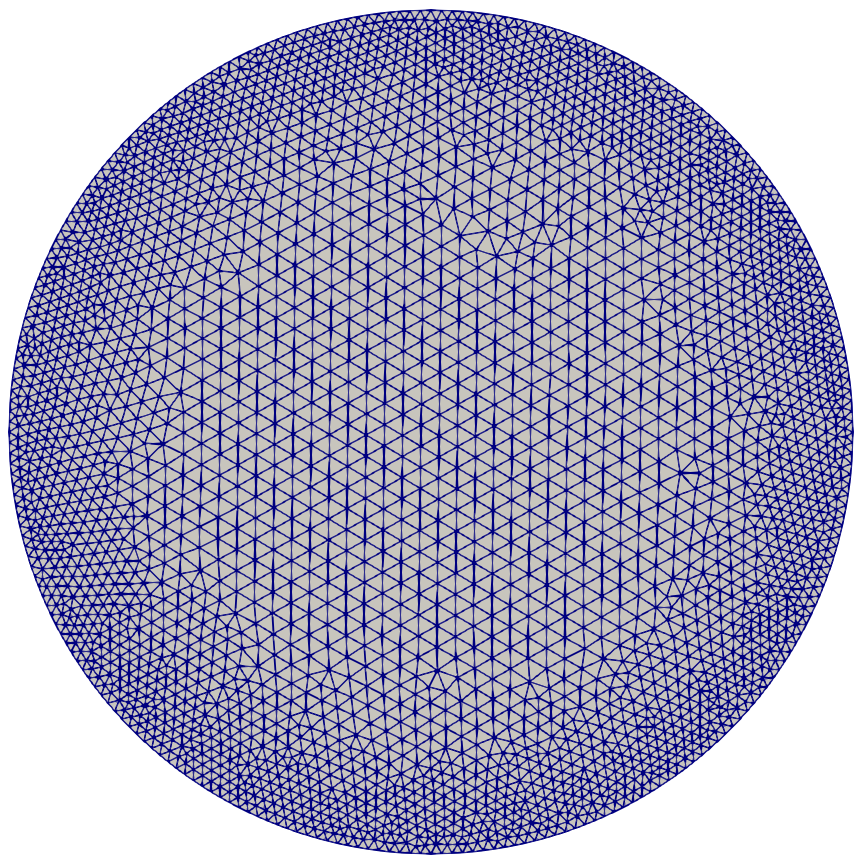
The approach outlined in Section 4 is chosen to obtain computational results based on a finite element discretization. Towards this goal, the disc $D$ is partitioned into a triangulation (mesh) of non overlapping triangular cells. We will refer to such triangulation as $D_{\delta}$ in the following. The triangulation is generated through gmsh [29], and contains 3219 nodes and 6438 cells. The mesh is unstructured, and is refined close to $\partial D$, i.e. to the elastic curve, ensuring that the cell size close to the boundary curve is approximately half of the mesh size at the origin of the disc, see Figure 1.

Refer to caption
Figure 1: Triangulation $D_{\delta}$ of the disc $D$, showing a mesh refinement on the boundary.

An approximation $\boldsymbol{X}_{\delta}$ of the membrane $\boldsymbol{X}$ is sought in a finite dimensional space $\mathcal{X}_{\delta}$ based on discontinuous Lagrange finite elements of degree 2 on triangles, i.e. the restriction of each component of $\boldsymbol{X}_{\delta}$ to any cell $T\in D_{\delta}$ is a second order polynomial. The finite element space $\mathcal{X}_{\delta}$ thus replaces the infinite dimensional space $W^{3,2}(D;\mathbb{R}^{3})$ in the formulation reported in Section 4. Concerning the approximation $\ell_{\delta}$ of the Lagrange multiplier $\ell$ in a finite dimensional space $\mathcal{L}_{\delta}$, we consider continuous Lagrange finite elements of degree 2 on segments. Such a finite dimensional approximation of $W^{\frac{1}{2},2}(\partial D;\mathbb{R})$ contains functions which are globally continuous and such that any element of $\mathcal{L}_{\delta}$ restricted to any boundary face of $D_{\delta}$ (i.e., any segment in the polygonal approximation $\partial D_{\delta}$ of $\partial D$) is a second order polynomial. There are two main differences between the finite dimensional spaces $\mathcal{X}_{\delta}$ and $\mathcal{L}_{\delta}$:

  1. 1.

    $\mathcal{X}_{\delta}$ is defined on the entire mesh $D_{\delta}$, while $\mathcal{L}_{\delta}$ is only defined over $\partial D_{\delta}$;

  2. 2.

    $\mathcal{X}_{\delta}$ is a space of local polynomials which are globally (possibly) discontinuous on $D_{\delta}$, while $\mathcal{L}_{\delta}$ is composed of local polynomials which are also globally continuous on $\partial D_{\delta}$.

Concerning the first consideration, it does not need to be justified any further, since it naturally stems from the corresponding infinite dimensional spaces $W^{3,2}(D;\mathbb{R}^{3})$ and $W^{\frac{1}{2},2}(\partial D;\mathbb{R})$, respectively. Regarding the choice of discontinuous elements for $\mathcal{X}_{\delta}$ in the second comment, it is strongly related to practical implementation limitations. Indeed, an approximation of $W^{3,2}(D;\mathbb{R}^{3})$ by means of continuous finite elements would actually require $C^{2}$ continuity across cells, rather than the standard $C^{0}$ continuity of Lagrange elements. Finite elements with high-order continuity are certainly less commonly studied than their corresponding standard counterparts; we mention here the Argyris triangle [3] or the Hsieh-Clough-Toucher triangle [18] as notable cases of elements with $C^{1}$ continuity. However, the implementation of finite elements with high-order continuity is not readily available in the FEniCS project [38], which we use for our numerical simulations together with the multiphenics [6] library, which easily allows to restrict the approximation $\ell_{\delta}$ of the Lagrange multiplier to just the boundary $\partial D_{\delta}$.

The finite element problem to be solved is: find $(\boldsymbol{X}_{\delta},\ell_{\delta})\in\mathcal{X}_{\delta}\times\mathcal{L}_{\delta}$ such that

$$\left\{\begin{aligned} &\mu\int_{D_{\delta}}\textgoth{C}\nabla\boldsymbol{X}_{\delta}:\nabla\boldsymbol{V}_{\delta}\,dudv+2\int_{\partial D_{\delta}}\partial_{\vartheta\vartheta}\boldsymbol{V}_{\delta}\cdot\partial_{\vartheta\vartheta}\boldsymbol{X}_{\delta}\,d\vartheta+2\int_{\partial D_{\delta}}\ell_{\delta}\;\partial_{\vartheta}\boldsymbol{V}_{\delta}\cdot\partial_{\vartheta}\boldsymbol{X}_{\delta}\;d\vartheta\\ &\qquad\underbrace{-\sum_{e\in E_{\delta}}\mu\int_{e}\left\{\!\!\left\{\textgoth{C}\nabla\boldsymbol{X}_{\delta}\right\}\!\!\right\}:\left[\!\left[\boldsymbol{V}_{\delta}\right]\!\right]\,de-\sum_{e\in E_{\delta}}\mu\int_{e}\left\{\!\!\left\{\textgoth{C}\nabla\boldsymbol{V}_{\delta}\right\}\!\!\right\}:\left[\!\left[\boldsymbol{X}_{\delta}\right]\!\right]\,de+\sum_{e\in E_{\delta}}\frac{\alpha}{h_{e}}\int_{e}\left[\!\left[\boldsymbol{X}_{\delta}\right]\!\right]\cdot\left[\!\left[\boldsymbol{V}_{\delta}\right]\!\right]\,de}_{\widetilde{\mathcal{D}}}\\ &\qquad\underbrace{+\varepsilon\int_{D_{\delta}}\boldsymbol{X}_{\delta}\cdot\boldsymbol{V}_{\delta}\;dudv}_{\widetilde{\mathcal{A}}}=0,\\ &\int_{\partial D_{\delta}}m_{\delta}\;\left[\left|\partial_{\vartheta}\boldsymbol{X}_{\delta}\right|^{2}-1\right]d\vartheta=0\end{aligned}\right.$$ (5.1)

for every $(\boldsymbol{V}_{\delta},m_{\delta})\in\mathcal{X}_{\delta}\times\mathcal{L}_{\delta}$. Eq. (5.1) is obtained from Eq. (4.8) by a standard Galerkin method on the finite dimensional space $\mathcal{X}_{\delta}\times\mathcal{L}_{\delta}$, with the addition of two new terms, denoted by $\widetilde{\mathcal{D}}$ and $\widetilde{\mathcal{A}}$.

The additional term $\widetilde{\mathcal{D}}$ appears due to the choice of discontinuous finite elements for $\mathcal{X}_{\delta}$, getting that the numerical scheme is a symmetric interior penalty discontinuous Galerkin method, see e.g. [23, 33, 46]. Here, $E_{\delta}$ is the set of all the interior edges in $D_{\delta}$ (i.e., the union of all segments $e\in\partial T$ for some $T\in D_{\delta}$, excluding the boundary edges $e\in\partial D_{\delta}$), $h_{e}$ is the length of an edge $e\in E_{\delta}$. For a fixed $e\in E_{\delta}$, let $T^{+}$ and $T^{-}$ be the two cells which share $e$ (i.e., $e=\overline{T^{+}}\cap\overline{T^{-}}$), and let $\mathbf{n}$ denote the outer normal to $e$ from $T^{+}$; then, the average $\left\{\!\!\left\{\cdot\right\}\!\!\right\}$ and jump $\left[\!\left[\cdot\right]\!\right]$ operators appearing in $\widetilde{\mathcal{D}}$ are defined as

$\displaystyle\left\{\!\!\left\{\textgoth{C}\right\}\!\!\right\}_{ij}$ $\displaystyle=\frac{\textgoth{C}_{ij}|_{T^{+}}+\textgoth{C}_{ij}|_{T^{-}}}{2},$
$\displaystyle\left[\!\left[\boldsymbol{X}\right]\!\right]_{ij}$ $\displaystyle=(\boldsymbol{X}_{i}|_{T^{+}}+\boldsymbol{X}_{i}|_{T^{-}})\mathbf{n}_{j}.$

Finally, $\alpha$ is a penalty coefficient (which we choose equal to $10^{4}$) which appears in the third addend in $\widetilde{\mathcal{D}}$ to penalize jumps of the solution across neighboring elements. One could also add further similar terms that penalize jumps of first and/or second order derivatives; such terms are often omitted (see e.g. [46]), since, with the proper choice of $\alpha$, our experience in the preparation of the results presented below is that a penalization on the jump of the polynomial solution results in practice in small jumps on its derivatives too.

The additional term $\widetilde{\mathcal{A}}$, instead, represents a penalization of the constraint (4.2), since such constraint is not enforced in the finite element space $\mathcal{X}_{\delta}$. In producing the numerical results which are discussed afterwards, we have experimentally observed that a small value $\varepsilon=10^{-5}$ is sufficient to prevent rigid body motions.

Remark 5.1 (On polynomial degree equal to 2).

We have seen in Section 4 that the presence of the term

$$2\int_{\partial D}\partial_{\vartheta\vartheta}\boldsymbol{V}\cdot\partial_{\vartheta\vartheta}\boldsymbol{X}\,d\vartheta$$

in Eq. (4.8) forces us to assume $\boldsymbol{X}\in W^{3,2}(D;\mathbb{R}^{3})$. As discussed above, this has profound numerical implications: we are forced to employ a discontinuous Galerkin method, primarily due to the unavailability of $C^{2}$ finite elements. Moreover, such a term implies the inability to use lowest order finite elements, i.e. polynomials of degree equal to 1. Indeed, $\partial_{\vartheta\vartheta}\boldsymbol{V}_{\delta}$ and $\partial_{\vartheta\vartheta}\boldsymbol{X}_{\delta}$ would otherwise be identically zero, and thus Eqs. (5.1) would ignore the boundary contribution to the energy functional.

Eqs. (5.1) result in a finite-dimensional quadratically nonlinear problem of total dimension 38355 degrees of freedom, of which 37851 for $\boldsymbol{X}_{\delta}$ and 504 unknowns for $\ell_{\delta}$. We solve such a nonlinear problem with the SNES solver, part of the PETSc library [5], with the following choices:

  • a backtracking procedure in the selection of the step length at every nonlinear iteration; in particular, SNES employs a cubic backtracking [5]. This procedure is beneficial in ensuring convergence of the nonlinear solver, as we have observed that simpler options (e.g., constant step length) often lead to divergence;

  • rescaling of the initial guess $\boldsymbol{X}_{guess}$ so that its perimeter is $2\pi$. This choice “helps" the numerical code to fulfil the nonlinear length preserving constraint. Indeed, we observed that providing an initial guess with considerably smaller or larger perimeters often resulted in stagnation to a nonconverged solution with the failure of the length preserving constraint, or even divergence.

The stopping criteria for the nonlinear iteration is realized by setting a suitable tolerance $\left(\hbox{approximately }<10^{-6}\right)$ under which we can deduce that the residual norm is very small, i.e. the discrete variational formulation is satisfied. Moreover, a posteriori, we check the constraints are fulfilled: the length of the solution $\boldsymbol{X}_{sol}$ at convergence must be close to $2\pi$ and the absolute value of the velocity $\left\lvert\boldsymbol{r}^{\prime}\right\rvert$ must be close to one.

We present next the numerical results obtained for two different choices for the linear elasticity tensor $\textgoth{C}$.

5.2 Identity tensor

First of all, we consider the case where the elastic tensor $\textgoth{C}$ coincides with the identity. In this section we choose different initial guesses $\boldsymbol{X}_{guess}$ for the parametrization, properly rescaled as discussed above, and we solve the nonlinear weak formulation as presented in Section 5.1. All the guesses are written in polar coordinates choosing $\varrho\in[0,1]$ to be the radial coordinate, while $\vartheta\in[0,2\pi]$ is the azimuth angular coordinate.

We consider as first guess datum $\boldsymbol{X}_{guess}$ a disc of radius one, whose formulation in polar coordinates is

$$\boldsymbol{X}_{guess}=(-\varrho\sin(\vartheta),\varrho\cos(\vartheta),0).$$

We expect not to be any variations since the disc is a critical point of the functional $\mathcal{E}_{n}$ defined in Eq. (4.3), i.e. we are starting “close enough" to a stationary solution. Indeed, the numerical solution $\boldsymbol{X}_{sol}$ is exactly the same disc, in the same plane, see Figure 2.

Refer to caption
Figure 2: Magnitude of the initial guess $\boldsymbol{X}_{guess}=(-\varrho\sin(\vartheta),\varrho\cos(\vartheta),0)$ (left), and of the corresponding obtained solution $\boldsymbol{X}_{sol}$ (right), which is in this case a circle.

We consider next

$$\boldsymbol{X}_{guess}=\left(\varrho\sin(\vartheta),\varrho\sin(\vartheta),\varrho\sin(\vartheta)\right)$$

as the second initial guess, which is the polar representation of an ellipse. Again in this case, see Figure 3, the numerical minimization converges to the disc in the same plane of the initial ellipse confirming that nonlinear iterations converge to a stable critical point when starting close enough to it.

Refer to caption
Figure 3: Magnitude of the initial guess $\boldsymbol{X}_{guess}=(\varrho\sin(\vartheta),\varrho\cos(\vartheta),\varrho\sin(\vartheta))$ (left), and of the corresponding obtained solution $\boldsymbol{X}_{sol}$ (center), which in this case is a circle. On the right, we plot the initial guess (in gray) and the obtained solution (colored) to show that they lay in the same plane.

Finally, we prescribe a non-planar initial guess: the paraboloid in Figure 4 is given by

$$\boldsymbol{X}_{guess}=\left(\varrho\cos(\vartheta),\varrho\sin(\vartheta),-\varrho^{2}\right).$$

Running the numerical code, we obtain as a critical point the disc in the plane passing through the maximum point $(0,0,0)$ and perpendicular to the axis of the paraboloid, that is the solution is progressively flattened on such a plane during the nonlinear iterations. Indeed, due to a change of sign in the curvature, any other configuration would cost more in terms of energy.

Refer to caption
Figure 4: Magnitude of the initial guess $\boldsymbol{X}_{guess}=(\varrho\cos(\vartheta),\varrho\sin(\vartheta),-\varrho^{2})$ (left), and of the corresponding obtained solution $\boldsymbol{X}_{sol}$ overlaid with the initial guess in grey (right) to show the plane which contains $\boldsymbol{X}_{sol}$.

To try to break the circular symmetry, we consider as initial guesses two ad hoc functions, i.e. in Figure 5 the initial guess is chosen to be

$$\boldsymbol{X}_{guess}=\left(\varrho\cos(\vartheta),-\varrho\sin(\vartheta),\varrho^{2}\sin^{2}(\vartheta)\right),$$

while, to plot Figure 6, we consider

$$\boldsymbol{X}_{guess}=\left(\varrho\cos(\vartheta),-\varrho\sin(\vartheta),\varrho^{2}\sin^{2}(\vartheta)+\sin\left(\frac{\pi}{2}\varrho\right)\cos(\vartheta)\right).$$

In both cases, a critical point is the disc. The interesting aspect is that, if in the previous results the lying plane of the disc can be deduced just by simple geometrical considerations, here the symmetry is broken. Indeed, we notice that increasing/decreasing the shear modulus $\mu$, such a plane changes.

Refer to caption
Figure 5: Magnitude of the initial guess $\boldsymbol{X}_{guess}=(\varrho\cos(\vartheta),-\varrho\sin(\vartheta),\varrho^{2}\sin^{2}(\vartheta))$ (left), and of the corresponding obtained solution $\boldsymbol{X}_{sol}$ (center), which in this case is a circle. On the right, we plot the initial guess (in gray) and the obtained solution (colored) to identify its position in $\mathbb{R}^{3}$ with respect to the initial guess.
Refer to caption
Figure 6: Magnitude of the initial guess $\boldsymbol{X}_{guess}=\left(\varrho\cos(\vartheta),-\varrho\sin(\vartheta),\varrho^{2}\sin^{2}(\vartheta)+\sin\left(\frac{\pi}{2}\varrho\right)\cos(\vartheta)\right)$ (left), and of the corresponding obtained solution $\boldsymbol{X}_{sol}$ (center), which in this case is a circle. On the right, we plot the initial guess (in gray) and the obtained solution (colored) to identify its position in $\mathbb{R}^{3}$ with respect to the initial guess..

Unfortunately, considering $\textgoth{C}$ as the identity tensor, we are not able to obtain critical points different from the disc. This motivates us to consider next an elasticity tensor $\textgoth{C}$ different from the identity.

5.3 Elasticity tensor different from the Identity Matrix

In this section, we choose different expressions for the linear elastic tensor $\textgoth{C}$, different from the identity. In particular, in Figure 7 its expression is

$$\textgoth{C}_{ijk\ell}=\delta_{ij}\delta_{k\ell}+2\left(1+10\sin^{2}(\varrho\cos(\vartheta))\right)\delta_{ik}\delta_{jl},$$

while in Figure 8 it is given by

$$\textgoth{C}_{ijk\ell}=\left\lvert\varrho\cos(\vartheta)\right\rvert\delta_{ij}\delta_{k\ell}+2\delta_{ik}\delta_{jl}.$$

The same initial condition $\boldsymbol{X}_{guess}$

$$\boldsymbol{X}_{guess}=\left(\varrho\cos(\vartheta),-\varrho\sin(\vartheta),\varrho\sin(\vartheta)+\sin\left(\frac{\pi}{2}\varrho\right)\cos(2\vartheta)\right),$$

is set in both cases.

We run the numerical simulations and we find, in both cases, critical points different from the disc. Precisely, the critical points present self-intersections. As discussed in the introduction, this is something that should be expected in minimizing the Dirichlet energy functional for the area contribution (see Chapter 8 of [40]) and thus we were set out to show in this work. The obtained solutions look profoundly different due to anisotropy effects in $\textgoth{C}$. Indeed, such choices of the linear elastic tensor favor different directions at which the stress will be maximum, thus resulting in two completely dissimilar solutions: a planar one with self-intersections in Figure 7 and a non-planar one with self-intersections in Figure 8.

Refer to caption
Figure 7: On the left, magnitude of the initial guess $\boldsymbol{X}_{guess}=\left(\varrho\cos(\vartheta),-\varrho\sin(\vartheta),\varrho\sin(\vartheta)+\sin\left(\frac{\pi}{2}\varrho\right)\cos(2\vartheta)\right)$ with $\textgoth{C}_{ijk\ell}=\left\lvert\varrho\cos(\vartheta)\right\rvert\delta_{ij}\delta_{k\ell}+2\delta_{ik}\delta_{jl}$ (colored), overlaid with the corresponding obtained solution $\boldsymbol{X}_{sol}$ in blue. We plot next the shape of $\boldsymbol{X}_{sol}$ (center) and its magnitude (right), resulting in planar self-intersections.
Refer to caption
Figure 8: Magnitude of the initial guess $\boldsymbol{X}_{guess}=\left(\varrho\cos(\vartheta),-\varrho\sin(\vartheta),\varrho\sin(\vartheta)+\sin\left(\frac{\pi}{2}\varrho\right)\cos(2\vartheta)\right)$ with $\textgoth{C}_{ijk\ell}=\delta_{ij}\delta_{k\ell}+2\left(1+10\sin^{2}(\varrho\cos(\vartheta))\right)\delta_{ik}\delta_{jl}$ (left), and of the corresponding obtained solution $\boldsymbol{X}_{sol}$ (right), which results in a non-planar solution with self-intersections.

6 Final remarks

The study of critical points for elastic functionals involve difficulties from both analytical and numerical points of view. In this work, we focus on such a energy type functionals

$$\mathcal{E}=\int_{\boldsymbol{\gamma}}f(\kappa,\tau)\,d\boldsymbol{\gamma}+\int_{D}\Psi(\nabla\boldsymbol{X})\,dudv,$$

where $f$ is an energy density function depending on the curvature and the torsion of the curve, $\Psi$ is a generic elastic energy density function defined on the disc which depends only on the gradient of the map $\boldsymbol{X}:D\to\mathbb{R}^{3}$ and the pointwise trace constraint holds.

If the critical point is a minimizer, the study we conducted is quite standard since we can directly apply the direct method of the Calculus of Variation with slightly more careful estimations required for the bound of $\left\lVert\boldsymbol{X}\right\rVert_{L^{2}}$ since the curve can self-intersect.

Looking for the first-order necessary conditions, comparing the two analytical introduced approaches, namely the parametrized and the framed curves one, we conclude that the best choice is the use of the infinite version of the Lagrange multipliers theorem, i.e. to rewrite everything in terms of the moving frame on the elastic curve. Indeed, since the problem is highly constrained, for the parametrized approach, we are forced to choose both $f$ and $\Psi$ to be linear functions, otherwise we are not able to get compactness.

For the numerical approach, we introduced a modified version of the parametrized approach which is more suitable for the discretization by means of a finite element method. In future, the proposed numerical approach can be used in biological researches. Indeed, the phenomenon of self-intersections can be interpreted as the physical absorption of knotted proteins by cellular membranes [26]. However, the proposed numerical approach can only penalize the curvature of the curve and consider linear elastic membrane. Future efforts must be devoted in developing a numerical method capable of handling the dependence of the energy density function $f$ on the torsion plus considering a non-linear elastic energy density $\Psi$, as introduced in the framed curve approach.

Acknowledgements

F.B. thanks the project Reduced order modelling for numerical simulation of partial differential equations funded by Università Cattolica del Sacro Cuore. The work of F.B. has been also partially supported by INdAM$-$GNCS, through the GNCS 2022 project Metodi di riduzione computazionale per le scienze applicate: focus su sistemi complessi. G.B. acknowledges support by Progetto d’Eccellenza 2018 – 2022 funded by Ministero dell’Università e della Ricerca (code: E11G18000350001) and G.B. was partially supported by INdAM$-$GNFM through the GNFM “Progetto Giovani" 2020 Transizioni di forma nella materia biologica e attiva. The work of L.L. has been partially supported by INdAM$-$GNAMPA. The work of A.M. has been also partially supported by INdAM$-$GNFM.

References

  • [1] E. Acerbi and N. Fusco. Semicontinuity problems in the calculus of variations. Archive for Rational Mechanics and Analysis, 86(2):125–145, 1984.
  • [2] F. J. Almgren. Existence and regularity almost everywhere of solutions to elliptic variational problems among surfaces of varying topological type and singularity structure. Annals of Mathematics, pages 321–391, 1968.
  • [3] J. H. Argyris, I. Fried, and D. W. Scharpf. The tuba family of plate elements for the matrix displacement method. The Aeronautical Journal, 72(692):701–709, 1968.
  • [4] M. Badiale and E. Serra. Semilinear Elliptic Equations for Beginners: Existence Results via the Variational Approach. Springer Science & Business Media, 2010.
  • [5] S. Balay, S. Abhyankar, M. F. Adams, S. Benson, J. Brown, P. Brune, K. Buschelman, E. Constantinescu, L. Dalcin, A. Dener, V. Eijkhout, W. D. Gropp, V. Hapla, T. Isaac, P. Jolivet, D. Karpeev, D. Kaushik, M. G. Knepley, F. Kong, S. Kruger, D. A. May, L. C. McInnes, R. T. Mills, L. Mitchell, T. Munson, J. E. Roman, K. Rupp, P. Sanan, J. Sarich, B. F. Smith, S. Zampini, H. Zhang, H. Zhang, and J. Zhang. PETSc/TAO users manual. Technical Report ANL-21/39 - Revision 3.17, Argonne National Laboratory, 2022.
  • [6] F. Ballarin. multiphenics - easy prototyping of multiphysics problems in FEniCS, 2016. https://mathlab.sissa.it/multiphenics.
  • [7] T. Belytschko. Selected works in applied mechanics and mathematics, 1996.
  • [8] F. Bernatzki and R. Ye. Minimal surfaces with an elastic boundary. Annals of Global Analysis and Geometry, 19(1):1–9, 2001.
  • [9] G. Bevilacqua, L. Lussardi, and A. Marzocchi. Soap film spanning electrically repulsive elastic protein links. Atti della Accademia Peloritana dei Pericolanti-Classe di Scienze Fisiche, Matematiche e Naturali, 96(S3):1, 2018.
  • [10] G. Bevilacqua, L. Lussardi, and A. Marzocchi. Soap film spanning an elastic link. Quarterly of Applied Mathematics, 77(3):507–523, 2019.
  • [11] G. Bevilacqua, L. Lussardi, and A. Marzocchi. Dimensional reduction of the Kirchhoff-Plateau problem. Journal of Elasticity, 140(1):135–148, 2020.
  • [12] G. Bevilacqua, L. Lussardi, and A. Marzocchi. Soap film spanning elastic boundaries. In preparation, 2022.
  • [13] G. Bevilacqua, L. Lussardi, and A. Marzocchi. Variational analysis of inextensible elastic curves. Proceedings of the Royal Society A, 478(2260):20210741, 2022.
  • [14] A. Biria and E. Fried. Buckling of a soap film spanning a flexible loop resistant to bending and twisting. Proceedings of the Royal Society A: Mathematical, Physical and Engineering Sciences, 470(2172):20140368, 2014.
  • [15] A. Biria and E. Fried. Theoretical and experimental study of the stability of a soap film spanning a flexible loop. International Journal of Engineering Science, 94:86–102, 2015.
  • [16] S. C. Brenner and L. R. Scott. The mathematical theory of finite element methods, volume 3. Springer, 2008.
  • [17] P. G. Ciarlet. The finite element method for elliptic problems. SIAM, 2002.
  • [18] R. W. Clough and J. L. Tocher. Finite element stiffness matricess for analysis of plate bending. In Proceedings of the Conference on Matrix Methods in Structural Mechanics,, pages 515–546, 1965.
  • [19] P. Creutz. Plateau’s problem for singular curves. arXiv preprint arXiv:1904.12567, 2019.
  • [20] A. Dall’Acqua, M. Novaga, and A. Pluda. Minimal elastic networks. arXiv preprint arXiv:1712.09589, 2017.
  • [21] G. David. Should we solve plateau’s problem again. Advances in Analysis: The Legacy of Elias M. Stein. Edited by Charles Fefferman, Alexandru D. Ionescu, DH Phong, and Stephen Wainger, 2014.
  • [22] C. De Lellis, F. Ghiraldin, and F. Maggi. A direct approach to plateau’s problem. Journal of the European Mathematical Society, 19(8):2219–2240, 2017.
  • [23] D. A. Di Pietro and A. Ern. Mathematical aspects of discontinuous Galerkin methods, volume 69. Springer Science & Business Media, 2011.
  • [24] J. Douglas. Solution of the problem of Plateau. Transactions of the American Mathematical Society, 33(1):263–321, 1931.
  • [25] A. Ern and J.-L. Guermond. Theory and practice of finite elements, volume 159. Springer, 2004.
  • [26] E. A. Evans. Mechanics and thermodynamics of biomembranes. CRC press, 2018.
  • [27] H. Federer and W. H. Fleming. Normal and integral currents. Annals of Mathematics, pages 458–520, 1960.
  • [28] H. Garcke, J. Menzel, and A. Pluda. Long time existence of solutions to an elastic flow of networks. Communications in Partial Differential Equations, 45(10):1253–1305, 2020.
  • [29] C. Geuzaine and J.-F. Remacle. Gmsh: A 3-d finite element mesh generator with built-in pre-and post-processing facilities. International journal for numerical methods in engineering, 79(11):1309–1331, 2009.
  • [30] L. Giomi and L. Mahadevan. Minimal surfaces bounded by elastic lines. Proceedings of the Royal Society A: Mathematical, Physical and Engineering Sciences, 468(2143):1851–1864, 2012.
  • [31] G. G. Giusteri, L. Lussardi, and E. Fried. Solution of the Kirchhoff–Plateau problem. Journal of Nonlinear Science, 27(3):1043–1063, 2017.
  • [32] O. Gonzalez, J. H. Maddocks, F. Schuricht, and H. von der Mosel. Global curvature and self-contact of nonlinearly elastic curves and rods. Calc Var, 14:29–68, 2002.
  • [33] J. S. Hesthaven and T. Warburton. Nodal discontinuous Galerkin methods: algorithms, analysis, and applications. Springer Science & Business Media, 2007.
  • [34] J. L. Lagrange. Essai dune nouvelle methods pour deteminer les maxima et les minima. Misc. Taur., 2:356–357, 1760.
  • [35] H. Le Dret and A. Raoult. Le modèle de membrane non linéaire comme limite variationnelle de l’élasticité non linéaire tridimensionnelle. Comptes rendus de l’Académie des sciences. Série 1, Mathématique, 317(2):221–226, 1993.
  • [36] H. Le Dret and A. Raoult. The nonlinear membrane model as variational limit of nonlinear three-dimensional elasticity. Journal de mathématiques pures et appliquées, 74(6):549–578, 1995.
  • [37] H. Le Dret and A. Raoult. The membrane shell model in nonlinear elasticity: a variational asymptotic derivation. Journal of Nonlinear Science, 6(1):59–84, 1996.
  • [38] A. Logg, K.-A. Mardal, and G. Wells. Automated solution of differential equations by the finite element method: The FEniCS book, volume 84. Springer Science & Business Media, 2012.
  • [39] A. Lytchak and S. Wenger. Area minimizing discs in metric spaces. Archive for Rational Mechanics and Analysis, 223(3):1123–1182, 2017.
  • [40] F. Morgan. Geometric measure theory: a beginner’s guide. Academic press, 2016.
  • [41] C. B. Morrey Jr. Quasi-convexity and the lower semicontinuity of multiple integrals. Pacific journal of mathematics, 2(1):25–53, 1952.
  • [42] B. Palmer and Á. Pámpano. Minimal surfaces with elastic and partially elastic boundary. Proceedings of the Royal Society of Edinburgh Section A: Mathematics, 151(4):1225–1246, 2021.
  • [43] A. C. Pipkin. The relaxed energy density for isotropic elastic membranes. IMA journal of applied mathematics, 36(1):85–99, 1986.
  • [44] J. Plateau. Experimental and theoretical statics of liquids subject to molecular forces only. Gauthier-Villars, Paris, 4, 1873.
  • [45] T. Radó. The problem of the least area and the problem of Plateau. Mathematische Zeitschrift, 32(1):763–796, 1930.
  • [46] B. Rivière. Discontinuous Galerkin methods for solving elliptic and parabolic equations: theory and implementation. SIAM, 2008.
  • [47] J. E. Taylor. The structure of singularities in soap-bubble-like and soap-film-like minimal surfaces. Annals of Mathematics, 103(3):489–539, 1976.
  • [48] E. Zeidler. Applied functional analysis: main principles and their applications, volume 109. Springer Science & Business Media, 2012.