Vahdat and Shashaani

Robust Output Analysis

Robust Output Analysis with Monte-Carlo Methodology

Kimia Vahdat kvahdat@ncsu.edu,
Edward P. Fitts Department of Industrial and Systems Engineering,
North Carolina State University
915 Partners Way, Raleigh, NC 27695 Sara Shashaani sshasha2@ncsu.edu,
Edward P. Fitts Department of Industrial and Systems Engineering,
North Carolina State University
915 Partners Way, Raleigh, NC 27695
https://shashaani.wordpress.ncsu.edu

In predictive modeling with simulation or machine learning, it is critical to accurately assess the quality of estimated values through output analysis. In recent decades output analysis has become enriched with methods that quantify the impact of input data uncertainty in the model outputs to increase robustness. However, most developments are applicable assuming that the input data adheres to a parametric family of distributions. We propose a unified output analysis framework for simulation and machine learning outputs through the lens of Monte Carlo sampling. This framework provides nonparametric quantification of the variance and bias induced in the outputs with higher-order accuracy. Our new bias-corrected estimation from the model outputs leverages the extension of fast iterative bootstrap sampling and higher-order influence functions. For the scalability of the proposed estimation methods, we devise budget-optimal rules and leverage control variates for variance reduction. Our theoretical and numerical results demonstrate a clear advantage in building more robust confidence intervals from the model outputs with higher coverage probability.

Monte-Carlo simulation; input uncertainty; model risk; bootstrap; non-parametric estimation

1 Introduction

Estimating the output of a predictive logic has been studied for many decades in the statistics, simulation, and machine learning (ML) literature. Model output error estimation is used for two primary purposes (Raschka 2018): (a) evaluating the performance of the predictive logic on unseen data (model generalization) and (b) adjusting for the settings of the predictive model and comparing different predictive modeling classes with each other.

Suppose that the model input denoted by $\bm{D}$, adheres to a true unknown distribution function $F_{0}$. The model output $Y=h(\bm{D},x)$ is an unknown functional of the model inputs and a control $x$ that is fixed and decided by the model user (see Figure 1). Let the quantity of interest be the expected output of a model under the true unknown distribution of inputs that feed into the model, $\theta(F_{0},x)=\mathbb{E}_{\bm{D}\sim F_{0}}[h(\bm{D},x)]$. Estimating $\theta(F_{0},x)$ well means the ability to generate a confidence interval of it with an experiment that is guaranteed to cover $\theta(F_{0},x)$ with high probability. Suppose $\hat{\theta}(F_{0},x)$ is the estimator along with the estimated $(1-\alpha)$% confidence interval $\mathcal{I}_{\alpha}(x)$. Then (a) implies that $\Pr\{\mathcal{I}_{\alpha}(x)\ni\theta(F_{0},x)\}\geq 1-\alpha$. Furthermore, (b) implies that if $x_{1}$ is a better choice for the model than $x_{2}$, i.e., $\theta(F_{0},x_{1})<\theta(F_{0},x_{2})$, then $\mathcal{I}_{\alpha}(x_{1})$ lies below $\mathcal{I}_{\alpha}(x_{2})$ with high probability. This is achieved by ensuring that the half-width of the two intervals is sufficiently narrow.

Figure 1: Diagram of model input-output relationship. Input data $\bm{D}$ is derived from a true unknown distribution, $F_{0}.$ The decision, $x,$ is entered to the model independently from the input data.

In simulation, $h$ is a physics-based logic and $\bm{D}$ feeds into it as a random (set of) vector-valued variable(s). In ML, $h$ is data-driven and with a fixed logic, i.e., linear regression, $\bm{D}$ is the training set that produces the predicted outcome under decision $x$. For both, one may be interested in a decision $x$ that outperforms others. The model parameters that best relay the input-output relationship in simulation (validation/calibration) or level of complexity in ML (model selection) can also be viewed as decisions. In this case, $h$ represents some loss function between the model generated outputs and the real observed values and $\bm{D}$ is two (likely non-overlapping) sets for training and validation.

We remark that a typical approach to ML is to build one prediction with one training (and validation) set. In the Monte Carlo (MC) framework, this means the expected value is estimated with the output of one replication, which is a bad estimator. Instead, guided by the MC principle, multiple replications of training (and validation) sets provide multiple possible predictions (e.g., via multiple regression lines and associated coefficients).

In all of the above, there is a risk in using the models discussed that corresponds to our uncertainty about the true input distribution $F_{0}$. In fact, any error in the choice of $F_{0}$ leads to shifting (bias) and scaling (variance) in the model outputs’ distribution. If both the bias and variance are quantified accurately enough, the goals in (a) and (b) can be achieved with more confidence. We term the added bias and variance to the model outputs as a result of uncertainty in the true input model $F_{0}$, the input uncertainty (IU) induced bias and variance.

While there is an extensive body of work for IU-induced variance and some recent attention to IU-reduced bias (Barton et al. 2022, Lam 2016, Song and Nelson 2019), the majority of these studies use parametric input models (Cheng and Holloand 1997, Morgan et al. 2019) that may be most relevant to small input spaces with variables that are infrequently assumed to be dependent. However, the larger simulation models and data-driven applications consist of larger input domains with complicated dependency structures for which the parameteric input models would be restrictive and unjustifiable. Nonparametric approaches to input uncertainty, while not explicitly designed for simulation applications, were developed in the statistical learning community are through the bootstrap (Chang and Hall 2015, Lam and Qian 2019, Barton et al. 2018).

The drawback of the existing bootstrap approaches is their laborious computation in loops of resampled data for learning/fitting especially for a good estimation of the bias in the outputs. One level of bootstrapped samples of the data would achieve an estimate of the bootstrap standard deviation for an empirical estimator $\hat{\theta}(x):=\theta(\hat{F},x)$, with $\hat{F}$ denoting the empirical distribution of $\{D_{i}\}_{i=1}^{n}$. To achieve an estimate of the inflated variance in the outputs due to IU, using (i) new bootstraps from each bootstrapped resample (nested bootstrap) (Barton et al. 2018) and (ii) empirical delta method (Lam and Qian 2019). (i) requires resampling and repeated model running for a sufficient number of times to approximation the resample distribution. (ii) has a high variance even for parametric approximations and even more for the nonparametric regime. Often the assumption of these studies, for $\hat{F}$ considered as a random distribution for a random set of data $\{D_{i}\}_{i=1}^{n}$ is that the bias term in

$$\theta(\hat{F})-\theta(F_{0})\approx\mathcal{N}(\text{bias},\text{ IU variance}+\text{expected MC variance})$$ (1)

is 0 (Song and Nelson 2019). (in the remainder of the paper $\hat{F}:=\hat{F}|\{D_{i}\}_{i=1}^{n}$ is considered fixed.) Although this assumption holds as $n\to\infty$, with either small samples or changing input generating functions, the bias can be a significant factor in the estimator’s error. In (1), the variance term comes from a simple decomposition and use of total variance law. We have also removed $x$ from the notation for ease of exposition.

In the presence of an accurate bias estimator, one can correct the estimator with $\hat{\theta}-\text{bias}$ before using it for inference or decision-making. However, compared to the variance, it is harder and more expensive to estimate the bias in either platform (simulation and ML). Parametric or nonparametric methods provide $\mathcal{O}(n^{-1})$ accuracy and often apply the bias directly to the confidence interval (by scaling/shifting the standard error or the critical value). Direct inference of the output bias or the bias of the estimator are not straightforward given the more realistic assumption of asymmetry in the outputs distribution. We explore estimating the bias using two non-parametric methods,(i) fast iterated bootstrapping (FIB), and (ii) higher order influence functions (HOIF). FIB (Ouysse 2013, Chang and Hall 2015) utilizes nested iterative bootstrapping to estimate the bias to the order of $\mathcal{O}(n^{-3/2})$ with controlled computation cost. We explore augmenting FIB with simulation output analysis bridging the fields of simulation and ML. HOIF takes another approach toward estimating the bias; it estimates the second-order sensitivity of the output towards changes in the input distribution. Achieving $\mathcal{O}(n^{-3/2})$ order of accuracy in the bias, which is slightly better than the variance term but important for small samples, seems elusive.

1.1 Contributions

We provide a framework for consistent and efficient quantification of IU-induced bias and variance with nonparametric input models. While our approaches are based on nested bootstrapping and nonparametric delta method, we devise efficient ways by which higher order of accuracy for the bias estimates can be achieved. In particular, we provide the following contributions:

• combining fast iterated bootstrapping, non-parametric delta methods, and $m$-out-of-$n$ subsampling for asymptotically unbiased bias estimators;

• bias correction for each output rather than the overall estimator to leverage common random numbers and variance reduction through a novel nested control variate from simulation analysis;

• minimizing the variance of the bias estimators using a multi-layer optimal budget allocation derived from nested simulation methodology; and

• proving the asymptotic validity of the resulting bias-corrected outputs’ CI.

We allow the framework to be unified for output analysis applicable to stochastic simulation and ML predictive modeling. To that end, we redefine the notion of output analysis for ML by generating multiple outputs for a given $x$, using a model trained with an input set $\bm{D}$. This view towards ML, while reminiscent to cross-validation and other existing techniques, is formalized here with a MC lens that enables our proposed approaches to be applicable for data-driven settings. We also develop a procedure for out-of-bag sampling in computing the ML model prediction error that incorporates the output bias and variance estimator.

During the development of our method, we became aware of a recently published non-parametric bias estimation method for stochastic optimization by Iyengar et al. (2023). They propose a bias estimator that utilizes a first-order influence function estimator. Their approach offers the advantage of not requiring additional model runs, resulting in improved efficiency. In our research, we also achieved a similar outcome by utilizing a closed-form second-order influence function estimator, in addition to improving the order of accuracy of bias estimation. By appropriately allocating our computational resources, we maintained the same total computing budget while providing an efficient bias estimator.

Ultimately, augmenting ML performance estimation with Monte Carlo-based output analysis increases the reliability and robustness of ML’s associated optimization routines for model construction. Correctly estimating CI for the outputs gives us more accurate performance measures for a given input, which can tremendously help compare solutions and increase robustness.

In the following section, we first illustrate the proposed method’s practicality concerning an inventory simulation problem. Section 3 covers the background literature on both ML and simulation techniques for output analysis. Section 4 defines the proposed estimator and demonstrates its statistical properties. Then, in Section 5, we elaborate on the nuances of ML model prediction estimation. Section 6 will compare the benefits of the proposed estimator with the existing benchmarks. Lastly, in Section 7, we conclude our discussion and point the interested audience to future research directions.

2 Illustrations – An inventory simulation

We now illustrate the impact of the proposed method on system performance estimate (goal (a)) and identification of the best alternative (goal (b)) in an inventory simulation example. Take an $(s,S)$ inventory system for which demand data observations exist. Let $n$ be the number of demand observations on-hand. We replicate the inventory system used in Koenig and Law (1985) with some modifications. The inventory policy in this system is to order up to $S$ when the on-hand inventory falls below $s$. For this example, the underlying demand distribution per period follows a Poisson distribution, which is unknown during the simulation. We generate two demand datasets for this illustration. In the first example, the demand is generated from a Poisson distribution, where the average is 30, without any noise, and in the second example, the data generating function is a Poisson with an average of 25 and nonzero mean integer noise, which has an average of 5. In both examples, the expected demand rate is 30, and a goodness of fit test ensures both demand data significantly follow the Poisson distribution. Also, a large warm-up period (10,000) is set for both examples to ensure the observed demand and cost are stabilized. From this point on, we will refer to the first example as “perfect Poisson” and the second as “corrupt Poisson”. The simulation logic is known, which generates the average total cost consisting of unit holding, ordering, and shortage costs over the simulation horizon (30 periods). In all the experiments, the total simulation budget (number of simulation runs) is fixed at 100, although the distribution of the budget differs across competing methods.

2.1 Goal (a): correct prediction

For a given scenario, i.e., fixed $(s,S)=(20,45)$, suppose we have observed demand and the total cost for $n$ periods and aim to test the accuracy of the 30-period simulation output CI by its likelihood of covering the true expected total cost. This will help the stakeholder obtain a more reliable expectation of the magnitude of incurred costs and more reliable comparisons between alternatives.

Conventionally, assuming that the distribution family of the demand is known, methods such as maximum likelihood estimator (MLE) can estimate its parameter, say $\hat{\rho}$ with the observed demands. Then, the fitted input model is incorporated into the simulation: the model produces replications of the output (expected total cost) under randomly generated inputs (demands) from the input model. We denote the simulation outputs with $Y_{r}(\hat{F}):=h(\hat{F}^{-1}(U_{r}),x)$, for $r=1,2,\ldots,R$ runs using $U_{r}\stackrel{{\scriptstyle iid}}{{\sim}}\text{Unif}(0,1)$ and $\hat{F}=F(\hat{\rho})$ to obtain $\bm{D}_{r}=\hat{F}^{-1}(U_{r}).$ The function $h(\cdot,x)$ yields the average total cost after 30 periods for the ordering policy $x$. Then the desired expected total cost is $\theta(\hat{F},x)=\mathbb{E}_{U}[h(\hat{F}^{-1}(U),x)]$ that can be estimated with $\hat{\theta}(\hat{F},x)=\bar{Y}(\hat{F}):=\frac{1}{R}\sum_{r=1}^{R}Y_{r}(\hat{F})$. We remark that using the data directly here and letting $\hat{F}$ be the empirical distribution makes the sample average value yield $\theta(\hat{F},x)$ and not its estimate. In this “crude” method, the CI of the expected value of interest, exploiting the central limit theorem (CLT), is estimated by $\bar{Y}(\hat{F})\pm t_{R-1,1-\alpha/2}\sqrt{\sum_{r=1}^{R}(Y_{r}(\hat{F})-\bar{Y}(\hat{F}))^{2}/(R-1)},$ where $t_{R-1,1-\alpha/2}$ is the student’s t-distribution critical value at $1-\alpha/2$ quantile.

However, the crude output analysis cannot quantify the increase in the outputs variance due to the uncertainty in the input model. When that variance increase is correctly quantified, the coverage of the estimated CIs increases. As summarized in Section 1, methods such as the nested simulation (Barton et al. 2018) that inflate the crude CI as a result of propagated input model error enhance the quality of the output analysis. This involves replacing $Y(\hat{F})$ with $Y(\hat{F}^{*})$ (in our example, $\hat{F}^{*}=F(\hat{\rho}^{*})$ – Poisson distribution with rate $\hat{\rho}^{*}$ computed from resamples with replacement). Because there is no guarantee that the bias effect on the outputs is the same across all input models and simulation runs, our proposed approach tracks the debiasing of each output separately as $\widehat{\text{bias}}_{r}(\hat{F})$ use bootstrapped resample distributions $\hat{F}^{*}$. Then we obtain $\hat{\theta}(F_{0})=\frac{1}{R}\sum_{r=1}^{R}(Y_{r}(\hat{F})-\widehat{\text{bias}}_{r}(\hat{F}))$.

Remark 2.1

Although we use a parametric input model and use bootstrapping, our main difference with the existing parametric methods for bias estimation Yang et al. (2021), Morgan et al. (2019, 2022), Song and Nelson (2019), Reichert and Schuwirth (2012) is that we do not use the difference between the input distributions with their parametric representations and instead compute those differences nonparametrically with empirical distributions. The proposed method will be described in Section 4. This clarifies that although the proposed methods can still be used in conjunction with parametric input models, its generality extends to larger input spaces with complex codependence structures where the empirical distribution will approximate their joint probability distributions.

Figure 2 demonstrates the effect of debiasing with the approach that we propose in this paper on the ability to predict in a range that covers the true average cost, $\frac{1}{30}\sum_{i=1}^{30}D_{i}$, where $D_{i}$ denotes the observed cost of the $i$-th period after the warm-up. Note that in both the simulation experiment and data generating process, we have set up a large warm-up period, 10,000 in these examples, to capture the long-run average cost. Interestingly, even if the true input distribution is not exactly Poisson, that is when we deliberately made an incorrect choice for the input model, the bias correction helps with recovering $\theta(F_{0})$ with the CI that covers the (approximated) expected average cost. Repeating this experiment with several input sizes reveals that in the crude method, the performance does not necessarily improve with larger $n$ due to the discrepancy between the fitted and actual distributions. The improvement due to increased input data size is evident in the IU-inflated in the case of perfect Poisson, but it is slow in the corrupt Poisson case. On the other hand, the bias-corrected CIs succeed in both cases and with all choices of $n$ in this experiment.

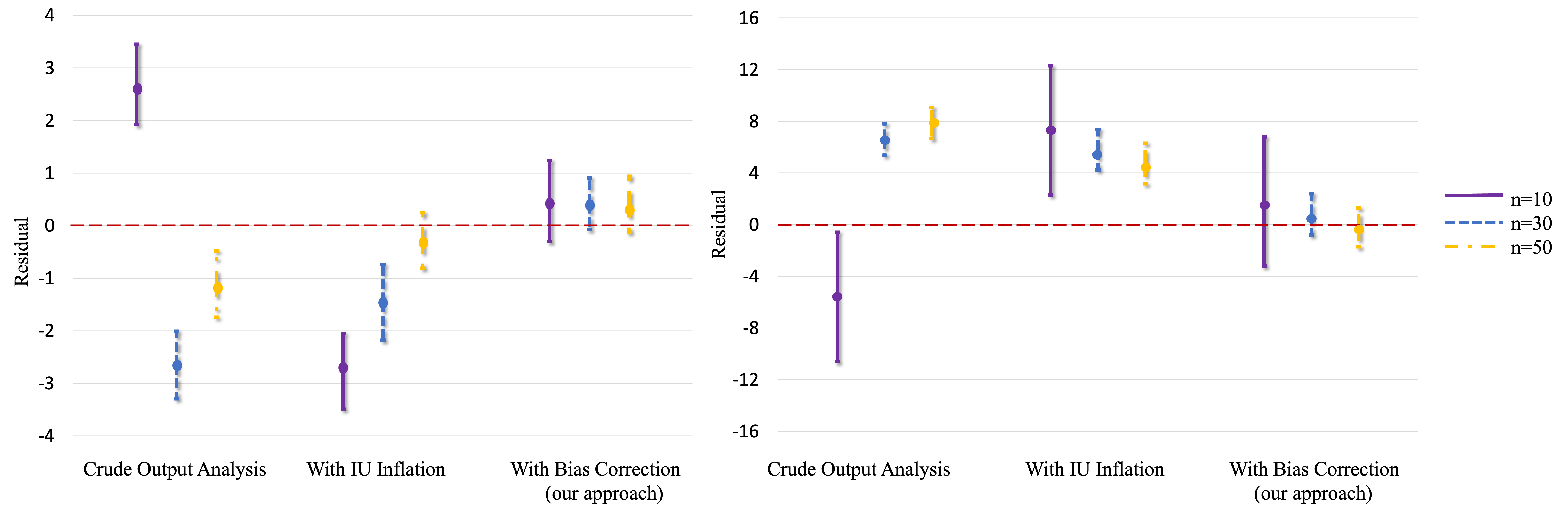
Figure 2: Three output analysis approaches are demonstrated over three input data sizes with $R=100$. The points represent the average difference between the estimated cost and the observed cost. The left panel shows the experiment with perfect Poisson. We observe that the CI are smaller than those in the corrupt Poisson case, in the right panel. Furthermore, the IU-inflated CI are able to encompass the true cost when $n$ is large in the perfect Poisson, which is not the case in the corrupt Poisson example.

2.2 Goal (b): correct comparison

We now compare our proposed debiasing method with the state-of-the-art bias and variance estimation methods in the simulation literature in terms of their ability to identify better alternatives. We demonstrate this by comparing the stationary trend between four $(s,S)$ scenarios (see Table 2.2), which is computed via 100 batch means of 30-period ($s,S$) inventory simulation runs, against those trends from the output analysis with different techniques. The synthetically generated long-run trend, generated by running the simulation model for 10,000 periods as a warm-up before collecting the target 30-period costs, with the batch means seeks to bury the dependence and nonstationarity in the outputs. Our goal is to recover the correct trend, which indicates that scenario 1 performs the best for both perfect and corrupt Poisson inputs. In the perfect Poisson use case, the order of preference is scenario 1, followed by scenarios 3, 4, and 2. Similarly, in the corrupt Poisson scenario, the order is scenarios 2, 3, and 4, following scenario 1.

The four scenarios of the $(s,S)$ inventory problem used for illustration II. The last two rows denote the expected cost with perfect Poisson, $F^{\text{p}}_{0}$, and the corrupt Poisson, $F^{\text{c}}_{0}.$ Scenarios 1 2 3 4 $s$ 20 20 20 20 $S$ 40 45 50 55 $\theta(F^{\text{p}}_{0})$ 179 191 188 189 $\theta(F^{\text{c}}_{0})$ 175 186 191 195

The experiment is run for a fixed 30-period simulation using two input demand sizes of 10 and 50 along with the mentioned corrupt and perfect Poisson datasets. The input demand data is used for estimating input distribution and the simulation output reports the average total cost over 30 periods. Figure 3 reveals that the bias-corrected CI successfully captures the correct trend, and more resoundingly so with $n=50$. The input distribution greatly affects the crude method, as it does not allow any room for errors caused by IU. The distance between the crude CI and the observed cost roughly shows the magnitude of bias, which is in fact significant. This distance is more misleading in the corrupt Poisson dataset and $n=10$, as it suggests scenario 2 has the minimum average cost, whereas scenario 1 has the least expected cost. The IU-inflated method performs better than the crude method; however, it is far from identifying the correct order between scenarios. Furthermore, in the case of corrupt Poisson and $n=10$, the IU-inflated CI distorts the relationship among scenarios 2, 3, and 4 by displaying scenario 2 as having the highest cost and scenario 4 as having the lowest cost. However, this is the exact opposite of the actual relationship between the expected costs of these scenarios. Even when the data size increases to 50, although the crude and IU-inflated CI difference from the true expected cost appears to decrease, the true trend is still not accurately captured.

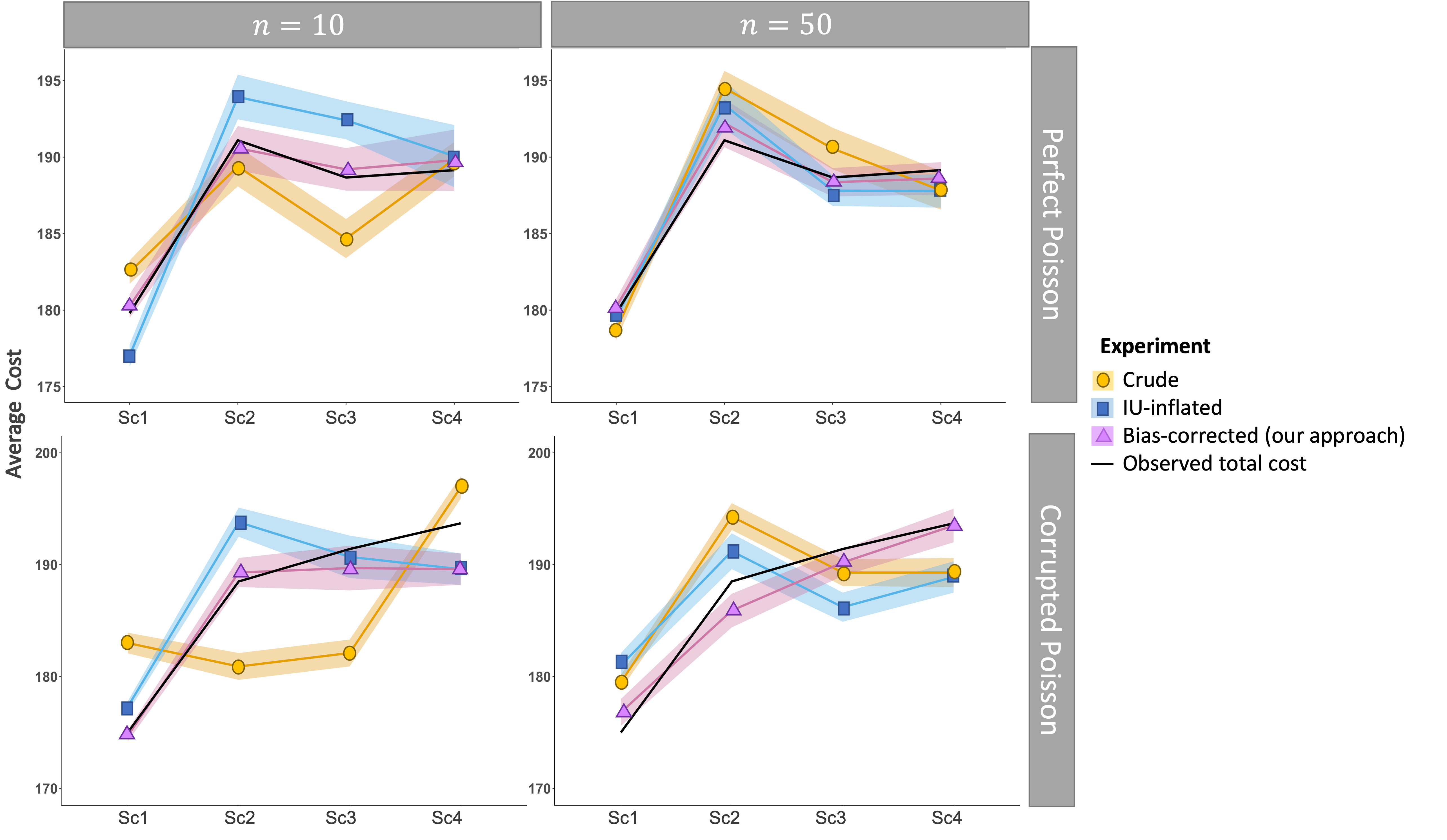
Figure 3: Comparing the 95% CI for two input data sizes and three competing methods for the perfect and corrupt Poisson input datasets. The top row shows the true cost and CI for the perfect Poisson, and the bottom row shows the corrupted case. The observed total cost is different across the two distributions because it depends on the input data.

The bias-corrected method, particularly when $n$ is limited, accurately estimates the bias and variance, and successfully identifies the correct system, as well as the ranking of all systems. This observation promises that even training the models or validating them with bias-corrected outputs could yield better models to emulate the truth. In the simulation model example, the logic has a parameter on the number of periods to discard for warm-up. This parameter needs to be tuned. Instead of searching for the best $(s,S)$ values, our objective can be to tune this parameter with the bias-corrected outputs. We leave that experimentation for the interested reader.

Before describing the proposed approach for direct bias-correction, we first lay out a more extensive review of the literature for output analysis in both simulation and ML.

3 Background

Before describing the proposed approach for direct bias-correction, we first lay out a more extensive review of the literature for output analysis in both simulation and ML.

3.1 Stochastic Simulation

Output analysis has been widely studied under parametric and non-parametric distributions in simulation systems (Lam 2016, Barton 2012). Parametric output analysis limits the data to a known family of distribution, which may fail to encompass the actual characteristics of the input data. Given a parametric input distribution, Morgan et al. (2019) compute an estimator for bias due to unknown input distribution for the simulation output. They achieve this by representing the simulation output as a function of the input distribution parameter. This allows them to rely on a vector of parameters to represent the input distribution. By employing Taylor expansion and central composite design around the MLE of the input parameter, they derive an estimator for the bias of the input distribution. However, their method does not generalize to non-parametric input models. Song and Nelson (2019) provide an extensive simulation output analysis under IU, where the bias and variance of the simulation models are studied considering parametric input models. They estimate the bias via a polynomial regression of degree 2 with data distribution parameters as independent variables. They show that the joint distribution between the input parameters and simulation output asymptotically follows a bi-variate normal, although with unclear validity for small data sizes ($n<50$). Yang et al. (2021) suggests another parametric approach towards deconvoluting the bias of IU in estimating a conditional expectation by debiasing the density of the input data Density deconvolution refers to fitting a density to noisy observed data by separating the noise from the density function.

Without any prior distributional assumption on the input data, there is one recent procedure to identify the bias due to input modeling. Iyengar et al. (2023) introduced a bias estimator that leverages the first-order functional derivation of the model output with respect to the empirical distribution, extending up to the order of $\mathcal{O}(n^{-1})$, to quantify the bias. They also require derivatives of the objective function, which in many practical cases is not available. This paper enhances the bias estimation with higher order IFs to $\mathcal{O}(n^{-2})$. There are some noteworthy studies on estimating the variance of the simulation model output. Davison and Hinkley (1997), Barton and Schruben (1993) and Barton and Schruben (2001) present sampling method for variance estimation. They suggest a nested simulation framework with bootstrapping to capture the data variability. Later Barton et al. (2018) present a variance reduction technique built on nested simulation framework to minimize the computation cost. Furthermore, Lam and Qian (2019) propose an alternative variance estimator using non-parametric delta methods, i.e., influence functions (IFs). They estimate the variability of the output with respect to small changes in the empirical input distribution. Unlike nested bootstrapping, estimating IU variance with IFs does not require additional model runs, which makes it efficient, particularly when it is expensive to run a model. On the other hand, they require some known distributional properties, which can be replaced with empirical distribution known properties.

Non-parametric estimation methods are better suited for high-dimensional settings and are more generalizable to various problems. However, they have some drawbacks. Non-parametric methods, usually based on data sampling, are computationally expensive, so they may not perform well for a limited computation budget (Fithian et al. 2014). The majority of computational burden arises due to the requirement of performing nested simulations. Nested simulations are computationally demanding due to resampling at the outer layer and running simulation runs per resampled input model at the inner layer. To control the overall error affected by input and simulation variations, a large number of simulation runs are required, multiplied by the sampling effort in each layer (Barton et al. 2022). In this paper, we propose an optimal allocation of the computation budget for the proposed bias and variance estimators, inspired by budget allocation in nested simulation studies (Lam and Qian 2021), to efficiently encompass the underlying uncertainty of the observed data into our estimation.

Another drawback of non-parametric methods in estimating the input distribution is their high dependence on the observed data (Lam 2021). We attempt to resolve this issue by implementing multi-level data sampling to reduce the dependency. More concretely, for $b_{1}=1,\cdots,B_{1}$ let the outputs of a simulation model with one level of sampling be, $\bar{Y}(\hat{F}^{*}_{b_{1}})=\frac{1}{R}\sum_{r=1}^{R}Y_{r}(\hat{F}^{*}_{b_{1}})$ and with two levels of sampling $\bar{\bar{Y}}(\hat{F}^{**}_{b_{1},.}),$ where

$$\bar{\bar{Y}}(\hat{F}^{**}_{b_{1},.})=\frac{1}{R}\frac{1}{B_{2}}\sum_{r=1}^{R}\sum_{b_{2}=1}^{B_{2}}Y_{r}(\hat{F}^{**}_{b_{1},b_{2}}).$$

While both sets of outputs have a dependency on the observed input data, the dependency of the latter set is intuitively less than the former. The reason is $\bar{\bar{Y}}(\hat{F}^{**}_{b_{1},.})$s are averaged over $B_{2}$ perturbations of $\hat{F}^{*}_{b_{1}}$ bootstrapped input model, mitigating the dependency on $\hat{F}$.

We have previously developed a bias estimator for the output of the stochastic simulation models using sampling-based methods and influence functions (Vahdat and Shashaani 2021). Nevertheless, the estimated bias was not practical due to high variability. In this paper, we build on the previous bias estimator and reduce its variance by employing the variance reduction techniques. Additionally, we estimate the bias for each individual simulation output using higher orders of IFs (HOIF). The variance of these IFs estimators is optimized using variance reduction techniques and optimal budget allocation. Furthermore, we combine HOIF with our proposed reduced variance FIB to enhance the stability of the final bias estimator. This paper also demonstrates the asymptotic unbiasedness of the proposed estimator and establishes valid confidence intervals for the model’s expected output. These confidence intervals are proven to asymptotically contain the true expected output with high probability.

The benefits of model output analysis considering IU are not limited to evaluating the simulation models. An exciting application of IU that has been of focus recently is distributionally robust optimization (DRO). In DRO, minimizing the expected output of a model, typically considered in simulation optimization settings, $\min_{x}\theta(F_{0},x)$, is converted to a min-max alternate, where the optimal solution is found within the worst-case in an uncertainty set, $\mathcal{F}$, i.e., $\min_{x}\sup_{F\in\mathcal{F}}\theta(F,x)$. The main challenge in DRO, similar to nonparametric delta method, is finding an unbiased and reliable estimate for $\nabla_{F}\theta(F,x)$. Ghosh et al. (2018) employ Giles’ debiased estimator for the gradient in training ML models. The Giles’ method (Giles 2008, Blanchet and Glynn 2015) is a practical way of debiasing a function of expected values, $\theta(F,x)$. However, it requires that the function does not have an unbiased estimator, hence it does not directly apply to sample average as an estimator of $\theta(F,x)$. Lam and Zhang (2021) provide an unbiased estimator of stochastic gradient descent using only a few sample observations. Their proposed estimator utilizes score functions to cancel out the higher-order bias terms without explicitly characterizing the bias. It is important to note that their method is only helpful when we want to estimate difference in $x_{1}$ and $x_{2}$, which is the case in finite-differencing for gradient approximation; it does not apply to a general case of estimation for a given $x$. In this paper, however, we introduce a bias estimator directly applicable to $\theta(F,x)$ that can be directly used to guide the optimization.

3.2 Machine Learning

The ML literature often does not recognize learning model outputs as a function of the unknown input data distribution. The existing body of work contains methods for a limited set of learning models, i.e., linear regression. Shao (1996) and Rabbi et al. (2021) introduce bootstrap-based confidence intervals for variable coefficients in linear regression that take the unknown input data into account. With the rise of black-box ML algorithms, there has been a new emphasis on model agnostic analysis, which, as its name suggests, is independent of the learning model (Efron 2020). Model agnostic output analysis relies primarily on “good” data sampling procedures that provide a robust estimate and addresses the conditional nature of the model output. Good data sampling is critical, especially when the magnitude of the desired performance is important.

$k-$fold cross-validation (Geisser 1975, Stone 1974), and several resampling methods such as $.632$ bootstrapping, double bootstrap, out-of-bag bootstrapping, and leave-one-out bootstrap or LOOBoot (Efron and Tibshirani 1997, Efron 1983) are well-known methods developed by statisticians and widely used for predictive model error analysis. $k-$fold cross-validation provides a balanced trade-off between bias and variance, with decreasing variance as the number of folds ($k$) increases. The bootstrapping method, which involves independently sampling training sets, yields low correlations between predictions and produces a small variance estimator. Efron (1983)’s thorough analysis and numerical experiments reveal that both $k-$fold cross-validation and the bootstrap converge at a rate of $\mathcal{O}(n^{-2})$. However, the bootstrap estimator introduces additional terms that contribute to a downward bias. Techniques such as LOOBoot can partially mitigate this bias, aiming to enhance the accuracy of results at the cost of onerous computation. It is worth noting that none of these methods have a closed-form equation for bias estimation for the outputs, though there are some bias estimators for confidence intervals (Hall 1986). For a more extensive review of the bootstrap-based model output estimation techniques, we refer the interested readers to a survey by Austin and Tu (2004). While these methods’ estimates may be good enough for general model comparisons, they fail to deliver a valid output CI. As noted, valid CI refers to confidence intervals that cover the true values with high likelihood, i.e., high coverage probability. We propose a novel bootstrap-based sampling method for quantifying the model’s performance, resulting in an asymptotically unbiased point estimator expected model output with IU-inflated variance, thus a more reliable CI with improved coverage probability.

Several studies in statistical analysis have introduced sampling-based estimators of bias. An interesting approach described by Chang and Hall (2015) and Ouysse (2013) is the double bootstrapping method, which involves perturbing the input data at two levels. The first level introduces perturbations to the data, while the second level varies the distributions obtained from the first level perturbations. This is directly linked to the use of the nested-simulation technique in stochastic simulation, which is employed to assess the variance of the input distribution. However, in multi-layer bootstrapping, the primary objective was to estimate the bias and enhancing the accuracy of the the output estimator. Notably, the second level in multi-layer sampling techniques within statistical analysis only requires a single replication. Despite the potential of these estimators, they are often overlooked in stochastic simulation settings due to their computationally expensive nature. In our research, we propose a solution to address this limitation by introducing a fixed-budget optimal allocation alongside our bias estimator. This approach effectively alleviates the computational burden associated with previous methods. Moreover, our proposed budget allocation strategy aims to minimize the variance of the bias estimator, thus ensuring the reliability of the bias estimates.

4 Proposed Methodology and Standing Assumptions

Denote the on-hand dataset with $\bm{D}:\{D_{i}\}_{i=1}^{n}$,each point of which represents one input data point. The objective is to estimate $\theta(F_{0})$ accurately despite that $F_{0}$ is unknown. With $Y(F_{0})$ as defined in Section 1, we can write

$$Y(F_{0})=\theta(F_{0})+\epsilon(F_{0}),$$

where $\epsilon(F_{0})$ is the MC error with mean 0 (Montgomery 2009). Given Assumptions 4 and  4, we aim to find an efficient and robust point estimator in addition to a valid CI for $\theta(F_{0}),$ where $F_{0}$ is not readily available. We call a CI valid, if its likelihood of containing $\theta(F_{0})$ converges to 1, as the computation effort goes to infinity. In other words, with a valid CI, we are able to provide an estimate of the true expected model output, even when the input data is limited.

For an input model $F$ that is fixed over time, $\theta(\cdot)$ is a smooth function of $F$. Simulation outputs are conditionally unbiased, i.e., for any input model $F$ $\mathbb{E}[Y(F)|F]=\mathbb{E}_{U}[h(F^{-1}(U))|F]=\theta(F),$ where $U\sim Unif(0,1),$ is a uniform random number.

In practice $F_{0}$ can be estimated with the empirical distribution of the data on hand, $\hat{F}=\frac{1}{n}\sum_{i=1}^{n}\delta_{\bm{D}}(D_{i})$, where $\delta_{\bm{D}}(D_{i})$ denotes the Dirac measure (takes value of 1, if $D_{i}\in\bm{D}$, and 0 otherwise) for point $D_{i}$. A point estimator for $\theta(\hat{F})$ is expressed as a sample average approximation (SAA) (Kleywegt et al. 2002) of $R$ simulation outputs, denoted by $Y_{r}(\hat{F})$ for $r=1,\cdots,R$. Here simulation refers to an iterative process of generating independent replications of $Y_{r}(\hat{F})$. Given Assumption 4, the crude point estimator for $\theta(\hat{F})$ is

$$\bar{Y}(\hat{F})=\frac{1}{R}\sum_{r=1}^{R}Y_{r}(\hat{F}).$$ (2)

Nevertheless, $\hat{F}$ is merely one realization of $F_{0},$ and $\hat{F}\neq F_{0}$ and consequently, $\theta(\hat{F})\neq\theta(F_{0}).$ Of course, the empirical CDF converges in distribution to $F_{0}$ at an exponential rate (Massart 1990), as $n$ tends to infinity. However, in many complex systems, either data is not readily available or using all of the data can be computationally expensive and we can opt for smaller subsets of data. Both cases results in $\beta(\hat{F}):=\theta(\hat{F})-\theta(F_{0})\neq 0,$ which induce an additional bias and variance into the estimation.

To capture the variability due to unknown input model, let $F$ be a random input model, then taking advantage of random effects model (Montgomery 2009, Ankenman and Nelson 2012) we expand the model output as a function of $F$, i.e.,

$$Y(F)=\theta(F_{0})+\left(\theta(F)-\theta(F_{0})\right)+\epsilon(F).$$

$$Y_{r}(F) =\theta(F)+\epsilon_{r}(F)$$

$$=\theta(F_{0})+\underbrace{\left(\theta(\hat{F})-\theta(F_{0})\right)}_{\beta(\hat{F})}+\underbrace{\left(Y_{r}(F)-Y_{r}(\hat{F})\right)}_{W_{r}(F)}+\epsilon_{r}(\hat{F}).$$ (3)

In (3), we take advantage of the observed realization of $F_{0},$ i.e., $\hat{F},$ to create an estimator for the model output. We define two sources of bias in (3). $\beta(\hat{F})$ is the discrepancy between the expected output given the empirical distribution and true input model, and $W_{r}(F)$ is the random bias at each simulation output level. By the expansion in (3), the MC error $\epsilon_{r}(F),$ is replaced with $\epsilon_{r}(\hat{F}),$ which has less variance due to $\hat{F}$ being fixed. Both bias terms can be negligible if the number of observed data points is large (Hall 1986). We exploit two methods of higher order IFs and FIB to estimate $\beta(\hat{F}),$ and $W_{r}(F),$ respectively.

Remark 4.1

Alternatively, another expansion for $Y_{r}(F)$ is,

$$Y_{r}(F)=\theta(F_{0})+\left(Y_{r}(\hat{F})-Y_{r}(F_{0})\right)+\left(Y_{r}(F)-Y_{r}(\hat{F})\right)+\epsilon_{r}(F_{0}),$$

in which the MC error, $\epsilon_{r}(\hat{F}),$ in (3) is replaced with $\epsilon_{r}(F_{0}).$ There are two main issues with directly estimating $Y_{r}(\hat{F})-Y_{r}(F_{0}).$ The first being, the smoothness requirement of HOIF could not have been met with each output, whereas by LLN we could claim the smoothness for $\theta.$ Secondly, we found out that estimating $Y_{r}(\hat{F})-Y_{r}(F_{0})$ would result in a highly variable bias estimator, which was not practical in ML examples.

We follow the bootstrap theory (Efron 1979), to imitate random input distributions from $\hat{F}$. We denote $\hat{F}^{*}_{1}:=\hat{F}^{*}(\zeta_{1})$. We generate $B_{1}$ input models, $\hat{F}^{*}_{1},\cdots,\hat{F}^{*}_{B_{1}}$, for each of which we generate $R$ simulation outputs. Then (3) can be written as

$$Y_{r}(\hat{F}^{*}_{b_{1}})=\theta(F_{0})+\beta(\hat{F})+W_{r}(\hat{F}^{*}_{b_{1}})+\epsilon_{r}(\hat{F}).$$

Section 4.2.1 will elaborate on how to take advantage of the bootstrap theory, namely,

$$\mathbb{E}_{\zeta}\left[\theta\left(\hat{F}^{*}(\zeta)\right)\right]-\theta(\hat{F})=\theta(\hat{F})-\theta(F_{0})+\mathcal{O}_{p}(n^{-1/2}),$$

with $\mathbb{E}_{\zeta}[\cdot]$ being the expectation with respect to the bootstraps perturbations, $\hat{F}^{*}(\zeta),$ and fast iterated bootstrapping to find an efficient estimator for $W_{r}(\hat{F}^{*}_{b_{1}})$ (Chang and Hall 2015, Ouysse 2013). The proposed estimator, $\hat{W}_{r}(\hat{F}^{*}_{b_{1}})$ reduces the bias up to $\mathcal{O}(n^{-3/2}),$ which can significantly impact the decisions in smaller datasets. Also, the bias $\beta(\hat{F})$ cannot be directly observed because only the empirical distribution is known and is fixed for a given subset of data. Section 4.2.2 provides a closed-form estimator for $\beta(\hat{F}),$ which we denote by $\hat{\beta}(\hat{F}),$ that uses a functional expansion around the empirical distribution (Van der Vaart 1998). Ultimately, estimating both bias terms, can improve our final estimator’s accuracy to $\mathcal{O}(n^{-2}).$

In addition to bias, estimating the total variance and each of its contributing components is critical in building a correct and valid CI and system diagnosis. When an estimate of each source of variability is known (stochastic noise or input data), one can effectively address the problematic component. For example, finding the input modeling process to contribute to the majority of variability can change the decision of conducting more simulation replications to collecting more data. Define the debiased point estimator as,

$$\bar{Y}^{d}(F)=\frac{1}{R}\sum_{r=1}^{R}Y_{r}(F)-\hat{\beta}(\hat{F})-\hat{W}_{r}(F),$$ (4)

where $\mathbb{E}_{U}[\bar{Y}^{d}(F)]=\theta(F_{0}).$ Then its variance, given Assumption 4 can be written as,

$$\text{Var}_{U,F}(\bar{Y}^{d}(F)) =\text{Var}_{U,F}\left(\bar{Y}(F)-\frac{1}{R}\sum_{r=1}^{R}\hat{W}_{r}(F)\right)$$

$$=\text{Var}\left(\bar{Y}(F)\right)+\text{Var}_{U,F}\left(\frac{1}{R}\sum_{r=1}^{R}\hat{W}_{r}(F)\right)-2\text{Cov}_{U,F}\left(\bar{Y}(F),\frac{1}{R}\sum_{r=1}^{R}\hat{W}_{r}(F)\right)$$

$$=\frac{\sigma^{2}_{U}}{R}+\text{Var}_{F}(\theta(F))+\text{Var}_{U,F}\left(\frac{1}{R}\sum_{r}\hat{W}_{r}(F)\right)-2\frac{R-1}{R}\text{Cov}_{U,F}\left(Y_{r}(F),\hat{W}_{r}(F)\right),$$ (5)

where the first term quantifies the simulation variance, the second term is the IU variance, and the last two terms are variances associated with bias estimation. In Equation (5), we expand $\text{Var}\left(\bar{Y}(F)\right)$ using the law of total variance, which involves conditioning on each source of uncertainty. For a detailed understanding of how this expansion works, refer to Remark 3. In Section 4.1, we further elaborate on how to estimate each component and how bias estimation affects the total variance. The variance of simulation output or stochastic uncertainty, i.e., $\sigma^{2}_{U},$ does not depend on its input model. Equivalently, $\mathbb{E}_{F}[\sigma^{2}_{U}(F)]=\sigma^{2}_{U}.$

Remark 4.2

Without debiasing, the total variance of the biased estimator, under Assumption 4, would be

$$\text{Var}(\bar{Y}(F)) =\mathbb{E}_{F}\left[\text{Var}_{U}\left(\bar{Y}(F)|F\right)\right]+\text{Var}_{F}\left(\mathbb{E}_{U}\left[\bar{Y}(F)|F\right]\right)=\frac{\sigma^{2}_{U}}{R}+\text{Var}_{F}(\theta(F)),$$ (6)

where the first and second term is the same as stochastic variance in (5). The difference between $\text{Var}(\bar{Y}(F))$ and (5) captures the increased variability due to bias estimation.

Steps to estimate the bias-corrected, IU-inflated, and crude CI are demonstrated. Figure 4 explains the algorithm for estimating $\hat{\beta}(\hat{F}^{*})$ and $\hat{\gamma}(\hat{F}^{*}).$ The role of two bias estimates are illustrated in the top row. The second row includes the IU variance into the CI, and the last row is the crude CI.

In the following subsections we detail the estimation methods for each term in (3). From this point on, for ease of exposition, we replace $\mathbb{E}_{\zeta}[.]$ with $\mathbb{E}_{*}[.]$ and similarly, $\text{Var}_{\zeta}(.)$ with $\text{Var}_{*}(.).$

The proposed iterated bootstrap estimator is demonstrated.

4.1 Variance Decomposition

This subsection provides an estimation for each term in (5) using $B_{1}$ bootstrap resamples drawn for characterizing the input model. Each $\hat{F}^{*}_{b_{1}}$ for $b_{1}=1,\cdots,B_{1}$ is the input distribution of a sampled data $\{D_{b_{1},i}\}_{i=1}^{n}$ drawn with replacement from $\hat{F}$. The resampled datasets are conditionally independent of each other, and the simulation process is repeated $R$ times for each. Relying on Assumption 4, estimating $\sigma^{2}_{U},$ becomes a straightforward task using sum of squared errors of all simulated outputs ($RB_{1}$ total model outputs). We begin by estimating $\text{Var}_{F}(\theta(F)),$ then discuss an ANOVA approach for estimating the variance of bias estimators.

With analysis of variance and bootstrap theory (Efron 1979) (see Remark 3), Barton and Schruben (2001), Lam (2016) estimate the input distribution variance, i.e., $\text{Var}_{F}(\theta(F)),$ with $\text{Var}_{*}(\theta(\hat{F}^{*}))$. Replacing random input models, $F,$ in (6) with bootstrapped distributions, $\hat{F}^{*},$ results in an estimator for IU variance as follows,

$$\widehat{\text{Var}}_{*}(\theta(\hat{F}^{*})) =\frac{1}{B_{1}-1}\sum_{b_{1}=1}^{B_{1}}\left(\bar{Y}(\hat{F}^{*}_{b_{1}})-\bar{Y}\right)^{2}-\frac{1}{R}\frac{1}{B_{1}(R-1)}\sum_{b_{1}=1}^{B_{1}}\sum_{r=1}^{R}\left(Y_{r}(\hat{F}^{*}_{b_{1}})-\bar{Y}(\hat{F}^{*}_{b_{1}})\right)^{2},$$ (7)

where $\bar{Y}(\hat{F}^{*}_{b_{1}})=\sum_{r=1}^{R}Y_{r}(\hat{F}^{*}_{b_{1}})/R$ and $\bar{Y}=\sum_{b_{1}=1}^{B_{1}}\bar{Y}(\hat{F}^{*}_{b_{1}})/B_{1}$. In (7) each variance is estimated with sum of squared residuals with respect to the variability source. We take advantage of their IU variance estimator directly in our total variance estimate.

Similar to the work of Barton and Schruben (2001), we calculate the sum of squared residuals of bias estimates and model outputs to find unbiased estimators for their variance and covariance terms. We conclude the total variance of the debiased estimator as,

$$\widehat{\text{Var}}(\bar{Y}^{d}(\hat{F}^{*})) =\frac{1}{R(B_{1}R-1)}\sum_{b_{1}=1}^{B_{1}}\sum_{r=1}^{R}\left(Y_{r}(\hat{F}^{*}_{b_{1}})-\bar{Y}\right)^{2}$$

$$+\frac{1}{B_{1}R(B_{1}R-1)}\sum_{b_{1}=1}^{B_{1}}\sum_{r=1}^{R}\left(\hat{W}_{r}(\hat{F}^{*}_{b_{1}})-\frac{1}{B_{1}}\sum_{b_{1}=1}^{B_{1}}\bar{W}(\hat{F}^{*}_{b_{1}})\right)^{2}$$

$$-\frac{2(R-1)}{B_{1}R^{2}(B_{1}R-1)}\sum_{b_{1}=1}^{B_{1}}\sum_{r=1}^{R}\left(\hat{W}_{r}(\hat{F}^{*}_{b_{1}})-\frac{1}{B_{1}}\sum_{b_{1}=1}^{B_{1}}\bar{W}(\hat{F}^{*}_{b_{1}})\right)\left(Y_{r}(\hat{F}^{*}_{b_{1}})-\bar{Y}\right)$$

$$+\frac{1}{B_{1}-1}\sum_{b_{1}=1}^{B_{1}}\left(\bar{Y}(\hat{F}^{*}_{b_{1}})-\bar{Y}\right)^{2}-\frac{1}{R}\frac{1}{B_{1}(R-1)}\sum_{b_{1}=1}^{B_{1}}\sum_{r=1}^{R}\left(Y_{r}(\hat{F}^{*}_{b_{1}})-\bar{Y}(\hat{F}^{*}_{b_{1}})\right)^{2},$$ (8)

where $\bar{W}(\hat{F}^{*}_{b_{1}})=\frac{1}{R}\sum_{r=1}^{R}\hat{W}_{r}(\hat{F}^{*}_{b_{1}}).$ Each estimated variance above identifies the contribution of its source (simulation, input data, or bias of input data) in the total variance and subsequently enhance the decision making. Next, we move onto estimating the biases introduced in Section 4

4.2 Bias Estimation

Besides computing the variance of the output, we also need to quantify the bias, as described in (3). Bias at the model output level can occur for two main reasons: the use of empirical distributions to quantify the error and the discrepancy between the true statistical and the estimated models. We only focus on the first bias term and leave the second one for future research.

In the previous section, in order to disintegrate the variance due to IU, we generated bootstrapped replications of the empirical distribution. We assume the expected model output is a smooth functional of input distribution and data observations are independent and identically distributed. Following the delta method a functional of the bootstrapped distributions converge to the functional of the actual distribution asymptotically, despite a non-negligible bias with limited simulation budget and data points (Van der Vaart 1998). In the subsequent sections, we explore the two methods of FIB and HOIF for estimating the bias terms defined in (4).

4.2.1 Fast Iterated Bootstrapping

We start by quantifying the bias due to bootstrapping, $W_{r}(\hat{F}^{*}_{b_{1}})$. Each simulation output given the sampled input is denoted by $Y_{r}(\hat{F}^{*}_{b_{1}})$ that is assumed to be a consistent estimator of $Y(\hat{F})$. We write the bootstrap estimate of bias as,

$$\bar{\Delta}_{r}^{*}(\hat{F}^{*}_{b_{1}}) =\widehat{\mathbb{E}}_{**}[Y_{r}(\hat{F}^{*}_{b_{1}})-Y_{r}(\hat{F})]=\frac{1}{B_{2}}\sum_{b_{2}=1}^{B_{2}}Y_{r}\left(\hat{F}_{b_{1},b_{2}}^{**}\right)-Y_{r}(\hat{F}^{*}_{b_{1}}),$$ (9)

where $B_{2}$ is the number of bootstrap resamples taken at each $B_{1}$ input models for identifying $W_{r}(\hat{F}^{*}_{b_{1}})$. Also, $\hat{F}^{**}_{b_{1},b_{2}}$ represents the sample distribution taken with replacement from $\hat{F}^{*}_{b_{1}}$. Note that in (9) the expectation is taken over another level of bootstrapping and hence the bias estimator itself is biased with the order of $\mathcal{O}(n^{-3/2})$ (Hall 1986).

Ouysse (2013) shows that we can estimate the bias of (9) with “fast” bootstrap sampling, while maintaining asymptotic convergence of standard bootstrapping. Fast bootstrapping means that only one sample is taken for the second level to reduce the computation cost. Let $\gamma_{r}\left(\hat{F}^{**}_{b_{1},.}\right)$ be the residual bias of $\bar{\Delta}_{r}^{*}(\hat{F}^{*}_{b_{1}})$ due to limited $B_{2}$, and $W_{r}(\hat{F}^{*}_{b_{1}})=\bar{\Delta}_{r}^{*}(\hat{F}^{*}_{b_{1}})+\gamma_{r}\left(\hat{F}^{**}_{b_{1},.}\right)$ be the total bias, then

$$W_{r}(\hat{F}^{*}_{b_{1}})=\mathbb{E}_{***}[Y_{r}\left(\hat{F}^{**}_{b_{1},.}\right)-Y_{r}(\hat{F}^{*}_{b_{1}})]=\bar{\Delta}^{*}_{r}\left(\hat{F}^{**}_{b_{1},.}\right)+\gamma_{r}\left(\hat{F}^{**}_{b_{1},.}\right),$$ (10)

where $\bar{\Delta}^{*}_{r}\left(\hat{F}^{**}_{b_{1},.}\right)=\widehat{\mathbb{E}}_{***}[Y_{r}\left(\hat{F}^{**}_{b_{1},.}\right)-Y_{r}(\hat{F}^{*}_{b_{1}})]$. Subtracting this equation from (10) achieves,

$$\hat{\gamma}_{r}\left(\hat{F}^{**}_{b_{1},.}\right) =\widehat{\mathbb{E}}_{***}[Y_{r}\left(\hat{F}^{**}_{b_{1},.}\right)-Y_{r}(\hat{F})]-\widehat{\mathbb{E}}_{***}[Y_{r}\left(\hat{F}^{**}_{b_{1},.}\right)-Y_{r}(\hat{F}^{*}_{b_{1}})]$$

$$=\frac{1}{B_{2}}\sum_{b_{2}=1}^{B_{2}}\left(Y_{r}\left(\hat{F}_{b_{1},b_{2}}^{***}\right)-Y_{r}\left(\hat{F}^{**}_{b_{1},b_{2}}\right)\right)-\frac{1}{B_{2}}\sum_{b_{2}=1}^{B_{2}}Y_{r}\left(\hat{F}_{b_{1},b_{2}}^{**}\right)+Y_{r}(\hat{F}^{*}_{b_{1}})$$

$$=\frac{1}{B_{2}}\sum_{b_{2}=1}^{B_{2}}Y_{r}\left(\hat{F}_{b_{1},b_{2}}^{***}\right)-\frac{2}{B_{2}}\sum_{b_{2}=1}^{B_{2}}Y_{r}\left(\hat{F}_{b_{1},b_{2}}^{**}\right)+Y_{r}(\hat{F}^{*}_{b_{1}}).$$

We define the fast iterated bootstrap corrected estimator as

$$Y^{d}_{r}(\hat{F}^{*}_{b_{1}})+\hat{\beta}(\hat{F}) =Y_{r}(\hat{F}^{*}_{b_{1}})-\hat{W}_{r}(\hat{F}^{*}_{b_{1}})$$

$$=Y_{r}(\hat{F}^{*}_{b_{1}})-\bar{\Delta}^{*}_{r}\left(\hat{F}^{**}_{b_{1},.}\right)-\hat{\gamma}_{r}\left(\hat{F}^{**}_{b_{1},.}\right)$$

$$=Y_{r}(\hat{F}^{*}_{b_{1}})+\frac{1}{B_{2}}\sum_{b_{2}=1}^{B_{2}}Y_{r}\left(\hat{F}_{b_{1},b_{2}}^{**}\right)-\frac{1}{B_{2}}\sum_{b_{2}=1}^{B_{2}}Y_{r}\left(\hat{F}_{b_{1},b_{2}}^{***}\right).$$ (11)

The $\hat{W}_{r}(\hat{F}^{*}_{b_{1}})=\bar{\Delta}^{*}_{r}\left(\hat{F}^{**}_{b_{1},.}\right)+\hat{\gamma}_{r}\left(\hat{F}^{**}_{b_{1},.}\right)$ is readily shown to be an unbiased estimator of the true bias of the model output given $\hat{F}^{*}_{b_{1}}$, via the law of large numbers. Ouysse (2013) proves that fast bias approximation converges to the actual bias with $\mathcal{O}(1/B_{2}),$ and Hall (1986) computes the error of the double iterated bootstrap to be of the order of $\mathcal{O}(n^{-3/2}).$ Lemma 4.3 summarizes these properties.

Lemma 4.3

Assume $\mathbb{E}[\hat{W}_{r}(\hat{F}^{*}_{b_{1}})^{3}]<\infty.$ By weak law of large numbers and bootstrap theory,

$$\big{|}\hat{W}_{r}(\hat{F}^{*}_{b_{1}})-W_{r}(\hat{F}^{*}_{b_{1}})\big{|}=\mathcal{O}_{p}(1/B_{2}).$$

Significance Test for FIB Bias Estimator: To further enhance the robustness of the proposed estimator, we conduct a statistical significance test using the central limit theorem and asymptotic properties of bootstrapping. We introduce a pivotal statistic,

$$T=\frac{\bar{\Delta}_{r}^{*}(\hat{F}^{**}_{b_{1},.})+\hat{\gamma}_{r}(\hat{F}^{**}_{b_{1},.})-W_{r}(\hat{F}^{*}_{b_{1}})}{\sqrt{\frac{1}{B_{2}-1}\sum_{b_{2}=1}^{B_{2}}\left(\Delta^{*}_{r}(\hat{F}^{**}_{b_{1},b_{2}})+\hat{\gamma}_{r}(\hat{F}^{**}_{b_{1},b_{2}})-\hat{W}_{r}(\hat{F}^{*}_{b_{1}})\right)^{2}}},$$ (12)

which follows student’s t distribution.

Theorem 4.4

Assuming standard regularity conditions, the pivotal statistic in (12) follows an asymptotic student’s t distribution. Subsequently

$$\lim_{B_{2}\to\infty}\mathbb{P}\left\{T_{\text{min}}(\alpha)\leq W_{r}(\hat{F}^{*}_{b_{1}})\leq T_{\text{max}}(\alpha)\right\}=1-\alpha,$$

where

$$T_{\text{max}}(\alpha)=\bar{\Delta}^{*}_{r}(\hat{F}^{**}_{b_{1},.})+\hat{\gamma}_{r}(\hat{F}^{**}_{b_{1},.})+t_{B_{2}-1,\alpha/2}\sqrt{\frac{1}{B_{2}-1}\sum_{b_{2}=1}^{B_{2}}\left(\Delta^{*}_{r}(\hat{F}^{**}_{b_{1},b_{2}})+\hat{\gamma}_{r}(\hat{F}^{**}_{b_{1},b_{2}})-\hat{W}_{r}(\hat{F}^{*}_{b_{1}})\right)^{2}},$$

and

$$T_{\text{min}}(\alpha)=\bar{\Delta}^{*}_{r}(\hat{F}^{**}_{b_{1},.})+\hat{\gamma}_{r}(\hat{F}^{**}_{b_{1},.})-t_{B_{2}-1,\alpha/2}\sqrt{\frac{1}{B_{2}-1}\sum_{b_{2}=1}^{B_{2}}\left(\Delta^{*}_{r}(\hat{F}^{**}_{b_{1},b_{2}})+\hat{\gamma}_{r}(\hat{F}^{**}_{b_{1},b_{2}})-\hat{W}_{r}(\hat{F}^{*}_{b_{1}})\right)^{2}},$$

where $t_{B_{2}-1,\alpha/2}$ is the $\alpha/2$ quantile of student’s t distribution with $B_{2}-1$ degrees of freedom.

Reduced Variance FIB Bias Estimator: The proposed bias estimator takes advantage of two layers of resampling, which can increase the variance of the estimator. In this subsection, we explore a variance-reduced version of $\hat{W}_{r}(\hat{F}^{*}_{b_{1}})$ using the control variate technique (Glasserman (2004), chapter 4). The control variate is a variance reduction technique that adds a multiplier of a centered correlated variable, with a known expectation, to the estimator (Ross 2022). The variance-reduced estimator improves the coverage probability by providing a less variable estimate of bias. We set the control variate as

$$C_{r}(\hat{F}^{*}_{b_{1}})=Y_{R+1}(\hat{F}^{*}_{b_{1}})-Y_{r}(\hat{F}^{*}_{b_{1}}),$$

where $Y_{R+1}(\hat{F}^{*}_{b_{1}})$ is a model output generated from a seed that is independent from random seeds generating outputs $Y_{1}(\hat{F}^{*}_{1}),\cdots,Y_{R}(\hat{F}^{*}_{b_{1}}).$ Note that, $\mathbb{E}[C_{r}(\hat{F}^{*}_{b_{1}})]=0$ as both terms are outputs of the same simulation model.

Hence, the variance-reduced bias estimator will be (for a given $b_{1}$ and $r$)

$$\hat{W}^{\text{cv}}_{r}(\hat{F}^{*}_{b_{1}},c_{1})=\hat{W}_{r}(\hat{F}^{*}_{b_{1}})+c_{1}C_{r}(\hat{F}^{*}_{b_{1}}),$$ (13)

where $c_{1}$ is a constant multiplier called coefficient of variation. The optimized coefficient of variation can be found by minimizing the variance of $\hat{W}^{\text{cv}}_{r}(\hat{F}^{*}_{b_{1}})$ with respect to $c_{1}.$ With some simple calculation we can see that the desired minimizer is $c_{1}^{*}=\text{Cov}(\hat{W}_{r}(\hat{F}^{*}_{b_{1}}),C_{r}(\hat{F}^{*}_{b_{1}}))/\text{Var}(C_{r}(\hat{F}^{*}_{b_{1}})).$ Note that, $c_{1}^{*}$ is not directly attainable, but can be estimated via

$$\hat{c}_{1}^{*}=\frac{\sum_{r=1}^{R}\left(\hat{W}_{r}(\hat{F}^{*}_{b_{1}})-\sum_{r=1}^{R}\hat{W}_{r}(\hat{F}^{*}_{b_{1}})/R\right)\left(C_{r}(\hat{F}^{*}_{b_{1}})-\bar{C}(\hat{F}^{*}_{b_{1}})\right)}{\sum_{r=1}^{R}\left(C_{r}(\hat{F}^{*}_{b_{1}})-\bar{C}(\hat{F}^{*}_{b_{1}})\right)^{2}},$$

where $\bar{C}(\hat{F}^{*}_{b_{1}})=\sum_{r=1}^{R}C_{r}(\hat{F}^{*}_{b_{1}})/R.$ As $R$ tends to infinity, by the law of large numbers, $\hat{c}_{1}^{*}$ converges to $c^{*}_{1}$ with probability 1. Nevertheless, substituting $c_{1}^{*}$ with its estimator induces a bias in the order of $\mathcal{O}(1/R)$ to $\hat{W}^{\text{cv}}_{r}(\hat{F}^{*}_{b_{1}},c_{1}^{*})$ (Glasserman 2004, Nelson 1990). Lemma 4.5 concludes that the bias of the variance-reduced FIB bias estimator converges to 0, as the computational effort, i.e., $B_{2}$ and $R$, grows large.

Lemma 4.5

By Lemma 4.3 and triangle inequality, we have

$$\mathbb{E}\left[\big{|}\hat{W}^{\text{cv}}_{r}(\hat{F}^{*}_{b_{1}},\hat{c}^{*}_{1})-W_{r}(\hat{F}^{*}_{b_{1}})\big{|}\right] =\mathbb{E}\left[\big{|}\hat{W}_{r}(\hat{F}^{*}_{b_{1}})+\hat{c}^{*}_{1}C(\hat{F}^{*}_{b_{1}})-W_{r}(\hat{F}^{*}_{b_{1}})\big{|}\right]$$

$$\leq\mathbb{E}\left[\big{|}\hat{W}_{r}(\hat{F}^{*}_{b_{1}})-W_{r}(\hat{F}^{*}_{b_{1}})\big{|}\right]+\mathbb{E}\left[\big{|}\hat{c}^{*}_{1}C(\hat{F}^{*}_{b_{1}})\big{|}\right]$$

$$=\mathcal{O}(\frac{1}{B_{2}})+\mathcal{O}(\frac{1}{R}).$$

The variance-reduced final estimator of the model output (see (11)) becomes

$$\bar{Y}^{d,\text{cv}}_{r}(\hat{F}^{*}_{b_{1}})+\hat{\beta}(\hat{F}) =Y_{r}(\hat{F}^{*}_{b_{1}})-\hat{W}^{\text{cv}}_{r}(\hat{F}^{*}_{b_{1}},\hat{c}^{*}_{1})$$

$$=Y_{r}(\hat{F}^{*}_{b_{1}})+\frac{1}{B_{2}}\sum_{b_{2}=1}^{B_{2}}Y_{r}\left(\hat{F}_{b_{1},b_{2}}^{**}\right)-\frac{1}{B_{2}}\sum_{b_{2}=1}^{B_{2}}Y_{r}\left(\hat{F}_{b_{1},b_{2}}^{***}\right)-\hat{c}^{*}_{1}(Y_{R+1}(\hat{F}^{*}_{b_{1}})-Y_{r}(\hat{F}^{*}_{b_{1}})).$$ (14)

4.2.2 Higher Order Influence Functions

In this subsection, we quantify $\beta(\hat{F})=\theta(\hat{F})-\theta(F_{0})$ using Von-Mises expansion and influence functions (Van der Vaart 1998). Von-Mises expansion is similar to the Taylor expansion with some modifications; define the function $\phi:t\to\theta(F+t(\hat{F}-F_{0})\sqrt{n})$. We estimate $\phi(t)$ at $t=0$ using the Taylor expansion as,

$$\theta(F+t(\hat{F}-F_{0})\sqrt{n})=\theta(F_{0})+t\nabla_{F}\theta(\hat{F}-F_{0})\sqrt{n}+\frac{nt^{2}}{2}\nabla^{2}_{F}\theta(\hat{F}-F_{0})^{2}+\mathcal{O}((t\|\hat{F}-F_{0}\|\sqrt{n})^{3}),$$

where $\nabla_{F}\theta$ and $\nabla^{2}_{F}\theta$ are the first and second order directional derivatives of $\theta$. In Von-Mises expansion, $t$ is replaced with $1/\sqrt{n}$ which results in,

$$\theta(\hat{F})=\theta(F_{0})+\nabla_{F}\theta(\hat{F}-F_{0})+\frac{1}{2}\nabla^{2}_{F}\theta(\hat{F}-F_{0})^{2}+\mathcal{O}(\|\hat{F}-F_{0}\|^{3}).$$ (15)

Assuming a linear and continuous first-order derivative, we have $\mathbb{E}[\nabla_{F}\theta(\hat{F}-F_{0})]=\nabla_{F}\theta(\mathbb{E}_{F}[\hat{F}-F])=0$. Hence, taking an expectation with respect to $F_{0}$ from (15) yields $\mathbb{E}[\theta(\hat{F})-\theta(F_{0})]\approx\mathbb{E}[\nabla^{2}_{F}\theta(\hat{F}-F_{0})^{2}]/2.$

Provided that the desired functional is smooth, i.e. infinitely many differentiable, Efron (2014) shows that based on the bootstrap theory $\|\hat{F}^{*}-\hat{F}\|\to\|\hat{F}-F_{0}\|$ as the number of data points grow large, and similarly, $\theta(\hat{F}^{*})-\theta(\hat{F})\to\theta(\hat{F})-\theta(F_{0})$. The smoothness assumption is valid in our case because $\theta$ is the expectation of model error. Employing the smoothness of $\theta$, we can estimate its first and second-order derivatives using the bootstraps already created for variance estimation. Consequently, we rewrite (15) using the empirical distribution and its random perturbation, $\hat{F}^{*}$.

Each $\hat{F}^{*}_{b_{1}}$ for $b_{1}=1,\cdots,B_{1}$, as explained in Section 4.1, is sampled from the empirical distribution of the on-hand dataset, $\hat{F}$, with replacement and size $m\leq n$. As noted by Lam and Qian (2021), sampling less than the on-hand data size will help manage the computation cost while controlling the variance. We point out additional advantages of sub-sampling in ML application in Section 5.

Define the probability of selecting point $i$ in $\hat{F}^{*}_{b_{1}}$ as $N_{b_{1},i}/n$, where

$$N_{b_{1},i}=\#\{\bm{D}_{b_{1}}=D_{i}\}\sim\text{binomial}(m,\bm{p}_{0})$$ (16)

is the number of repeated samples of $D_{i}$ in $\bm{D}_{b_{1}}$. In (16), $\bm{p}_{0}=(1/n,\cdots,1/n)$, and $\bm{N}_{b_{1}}\sim$Mult$(m,\bm{p}_{0})$. Additionally, $\bm{D}_{b_{1}}$ represents the $b_{1}$-th sample taken from $\bm{D}$. Note that $\hat{F}$ and $\hat{F}^{*}$ can be written as $\frac{1}{n}\sum_{i=1}^{n}\delta(D_{i})$ and $\frac{1}{m}\sum_{i=1}^{n}N_{b_{1},i}$, respectively. Then the Von-Mises expansion for an arbitrary $b_{1}$ is,

$$\theta\left(\hat{F}^{*}_{b_{1}}\right) =\theta(\hat{F})+\sum_{i=1}^{n}\nabla_{\hat{F}}\theta\left(\frac{N_{b_{1},i}}{m}-\frac{\delta(D_{i})}{n}\right)+\frac{1}{2}\sum_{i=1}^{n}\sum_{j=1}^{n}\nabla^{2}_{\hat{F}}\theta\left(\frac{N_{b_{1},i}}{m}-\frac{\delta(D_{i})}{n}\right)\left(\frac{N_{b_{1},j}}{m}-\frac{\delta(D_{j})}{n}\right)$$

$$=\theta(\hat{F})+\sum_{i=1}^{n}\nabla_{\hat{F}}\theta\left(\frac{N_{b_{1},i}}{m}-\frac{1}{n}\right)+\frac{1}{2}\sum_{i=1}^{n}\sum_{j=1}^{n}\nabla^{2}_{\hat{F}}\theta\left(\frac{N_{b_{1},i}}{m}-\frac{1}{n}\right)\left(\frac{N_{b_{1},j}}{m}-\frac{1}{n}\right),$$

where the second equation simplifies the first by limiting the summation to the available data points and replacing $\delta$ with 1.

It remains to propose an unbiased estimator for $\nabla_{\hat{F}}\theta$ and $\nabla^{2}_{\hat{F}}\theta$. We employ score functions to develop the desired estimators. Lam and Qian (2019) propose an unbiased estimator for $\nabla_{\hat{F}}\theta$ at point $D_{i}$ using score functions,

$$\widehat{\text{IF}}_{1}\left(D_{i};\hat{F}\right) =\frac{1}{B_{1}}\sum_{b_{1}=1}^{B_{1}}\frac{1}{R}\sum_{r=1}^{R}Y^{d}_{r}\left(\hat{F}^{*}_{b_{1}}\right)S^{(1)}_{i}\left(\hat{F}^{*}_{b_{1}}\right),$$ (17)

where

$$S^{(1)}_{i}\left(\hat{F}^{*}_{b_{1}}\right)=\frac{n-1}{n\text{Var}(N_{b_{1},i}/m)}\left(\frac{N_{b_{1},i}}{m}-\frac{1}{n}\right)=mn\left(\frac{N_{b_{1},i}}{m}-\frac{1}{n}\right)$$

is the score function. They show that $\mathbb{E}[\widehat{\text{IF}}_{1}\left(D_{i};\hat{F}\right)|\hat{F}]=\nabla_{\hat{F}}\theta$, hence it is unbiased. We build on their approach to provide an unbiased estimator for $\nabla^{2}_{\hat{F}}\theta$, which then can be used for the bias estimation.

Note that $\nabla^{2}_{\hat{F}}\theta$ is a bilinear mapping, so for a given pair of distinct points $D_{i}$ and $D_{j}$, we define the estimator as,

$$\widehat{\text{IF}}_{2}\left(D_{i},D_{j};\hat{F}\right) =\frac{1}{B_{1}}\sum_{b_{1}=1}^{B_{1}}\frac{1}{R}\sum_{r=1}^{R}Y^{d}_{r}\left(\hat{F}^{*}_{b_{1}}\right)S^{(2)}_{i,j}\left(\hat{F}^{*}_{b_{1}}\right)+\frac{\lambda Y^{d}_{r}(\hat{F})}{mn^{2}}-\lambda\eta\widehat{\text{IF}}_{1}\left(D_{i};\hat{F}\right),$$ (18)

where

$$S_{i,j}^{(2)}\left(\hat{F}^{*}_{b_{1}}\right) =\lambda\left(\frac{N_{b_{1},i}}{m}-\frac{1}{n}\right)\left(\frac{N_{b_{1},j}}{m}-\frac{1}{n}\right),$$

$$\lambda \approx-1/5\text{Cov}\left(N_{b_{1},i}/m,N_{b_{1},j}/m\right),$$ (19)

and

$$\eta\approx 6\text{Cov}(N_{b_{1},i}/m,N_{b_{1},j}/m)+4\mathbb{E}[N_{b_{1},i}/m]^{3}.$$ (20)

Appendix 8 elaborates on derivation of (19) and (20). Note that calculating $S_{i,j}^{(2)}\left(\hat{F}^{*}_{b_{1}}\right)$, for all pairs of $(i,j)$, requires $n^{2}$ arithmetic computation, which grows large as the data size increases. This computation burden should be negligible in practice, since the proposed method’s main application is for smaller datasets, in which input data induced bias is significant.

The unbiasedness of the proposed estimator, denoted as $\widehat{\text{IF}}_{2}\left(D_{i},D_{j};\hat{F}\right)$, is established in Theorem 4.6 under the assumption of the empirical distribution.

Theorem 4.6

Assuming $\bar{Y}^{d}(.)$ being a smooth function of input distribution and $Y^{d}_{r}(\hat{F}^{*}_{b_{1}})$ are identically distributed and conditionally independent, $\widehat{\text{IF}}_{2}\left(D_{i},D_{j};\hat{F}\right)$ defined in (18) is an unbiased estimator of $\nabla^{2}_{\hat{F}}\theta$.

We can further expand the results of Theorem 4.6 and provide assurances regarding the convergence of the empirical CDF to the true distribution at an exponential rate Massart (1990). Particularly, as per initial assumptions $\theta$ is a smooth function of input distribution, therefore $\nabla^{2}\theta(.)$ is respectively a smooth function of the input distribution. Given $\nabla_{\hat{F}}^{3}\theta(.)<\infty$, we can apply the delta method and Glivenko-Cantelli theorem (Loève 1977) and achieve,

$$\mathbb{P}\left\{\lim_{n\to\infty}\sup_{D_{i},D_{j}}\bigg{|}\nabla^{2}_{\hat{F}}\theta(D_{i},D_{j})-\nabla^{2}_{F}\theta(D_{i},D_{j})\bigg{|}=0\right\}=1.$$

Hence the bias estimate can be written as,

$$\mathbb{E}_{*}[\theta(\hat{F}^{*})-\theta(\hat{F})] =\mathbb{E}_{*}\left[\frac{1}{2}\sum_{i=1}^{n}\sum_{j=1}^{n}\widehat{\text{IF}}_{2}(i,j;\hat{F})\left(\frac{N_{b_{1},i}}{m}-\frac{1}{n}\right)\left(\frac{N_{b_{1},j}}{m}-\frac{1}{n}\right)\right]$$

$$=\frac{1}{2}\mathbb{E}_{*}\Bigg{[}\sum_{i=1}^{n}\sum_{j=1}^{n}\frac{1}{R}\sum_{r=1}^{R}Y^{d}_{r}\left(\hat{F}^{*}\right)S^{(2)}_{i,j}\left(\hat{F}^{*}\right)\frac{S^{(2)}_{i,j}\left(\hat{F}^{*}\right)}{\lambda}$$

$$\ \ \ +\frac{S^{(2)}_{i,j}\left(\hat{F}^{*}\right)Y^{d}_{r}(\hat{F})}{mn^{2}}-\eta S^{(2)}_{i,j}\left(\hat{F}^{*}\right)\widehat{\text{IF}}_{1}\left(D_{i};\hat{F}\right)\Bigg{]}$$

$$=\frac{\lambda}{2}\sum_{i=1}^{n}\sum_{j=1}^{n}\mathbb{E}_{*}\left[\frac{1}{R}\sum_{r=1}^{R}Y^{d}_{r}\left(\hat{F}^{*}\right)\left(\frac{N_{b_{1},i}}{m}-\frac{1}{n}\right)^{2}\left(\frac{N_{b_{1},j}}{m}-\frac{1}{n}\right)^{2}\right]$$

$$=\frac{\lambda}{2}\sum_{i=1}^{n}\sum_{j=1}^{n}\text{Cov}_{*}\left(\frac{1}{R}\sum_{r=1}^{R}Y^{d}_{r}\left(\hat{F}^{*}_{b_{1}}\right),\left(\frac{N_{b_{1},i}}{m}-\frac{1}{n}\right)^{2}\left(\frac{N_{b_{1},j}}{m}-\frac{1}{n}\right)^{2}\right)+\mathcal{O}(m^{-2}n^{-4}).$$ (21)

We can show that as $n$ goes to infinity, the variance of $\widehat{\text{IF}}_{2}$ becomes unbounded (Var$(\widehat{\text{IF}}_{2})=\mathcal{O}(n^{5})$). This means that in smaller datasets, we achieve a more stable estimator of bias than in larger datasets, which is not detrimental as the bias decreases with more data points. However, we can further reduce the variance by utilizing the control variate technique. We use the $\widehat{\text{IF}}_{1}$ as the control variate statistic, since its expectation and variance are known. The control variate is our novelty in enhancing the HOIF bias estimator from its original variation in Efron (2014). It remains to compute the optimal coefficient of variance, that is equal to $c_{2}^{*}=-\text{Cov}(\widehat{\text{IF}_{2}}(\hat{F}),\widehat{\text{IF}_{1}}(\hat{F}))/\text{Var}(\widehat{\text{IF}_{1}}(\hat{F}))$.

Lemma 4.7

The optimal coefficient of variance $c_{2}^{*}=\frac{-\text{Cov}(\widehat{\text{IF}_{2}}(\hat{F}),\widehat{\text{IF}_{1}}(\hat{F}))}{\text{Var}(\widehat{\text{IF}_{1}}(\hat{F}))}$ can be approximate with $-0.2\left(n-\frac{1}{m}+\frac{2}{mn}+1\right)+\mathcal{O}(m^{-2}n^{-2})$ due to

$$\text{Cov}_{*}(\widehat{\text{IF}_{2}}(\hat{F}),\widehat{\text{IF}_{1}}(\hat{F})) =\frac{\bar{Y}(\hat{F})^{2}}{5}\left(2+mn-n+mn^{2}+\frac{6}{mn}-\frac{6}{mn^{2}}-\frac{4}{n^{2}}+\frac{4}{n^{3}}\right).$$

Here we drop the $D_{i}$ and $D_{j}$ from the influence function estimators to generalize the results for any point.

Following these results, the final bias estimator becomes for a given $b_{1}$ is

$$\hat{\beta}(\hat{F}) \approx\left(-1.2\text{Cov}(N_{b_{1},i}/m,N_{b_{1},j}/m)\right)$$

$$\ \ \ \times\sum_{i=1}^{n}\sum_{j=1}^{n}\text{Cov}_{*}\left(\frac{1}{R}\sum_{r=1}^{R}Y^{d}_{r}\left(\hat{F}^{*}_{b_{1}}\right),\left(\frac{N_{b_{1},i}}{m}-\frac{1}{n}\right)^{2}\left(\frac{N_{b_{1},j}}{m}-\frac{1}{n}\right)^{2}\right).$$ (22)

Remark 4.8

Viewing each bootstrapped sample as one simulation replication, the expected bias in (21) is the same as second order linear regression coefficient of outputs with respect to the empirical cdf. For more intuition refer to Lin et al. (2015).

We next prove in Theorem 4.9 that the total bias estimator, $\hat{\beta}(\hat{F})+\hat{W}(\hat{F}^{*}),$ converges to the true bias with probability 1, as the computation budget increases. Furthermore, Theorem 4.9 shows that similar convergence results can be achieved with the variance-reduced FIB bias estimator, introduced in (14).

Theorem 4.9

The variance-reduced total bias estimator defined as $\hat{W}^{\text{cv}}(\hat{F}^{*})+\hat{\beta}(\hat{F})$ and total bias estimator, namely $\hat{W}(\hat{F}^{*})+\hat{\beta}(\hat{F})$, are unbiased estimators of $W(\hat{F}^{*})+\beta(\hat{F}),$ i.e.,

$$\lim_{N\to\infty}\mathbb{E}\left[|\hat{W}(\hat{F}^{*})+\hat{\beta}(\hat{F})-W(\hat{F}^{*})-\beta(\hat{F})|\right]=\lim_{N\to\infty}\mathbb{E}\left[|\hat{W}^{\text{cv}}(\hat{F}^{*})+\hat{\beta}(\hat{F})-W(\hat{F}^{*})-\beta(\hat{F})|\right]=0,$$

where $N=B_{1}RB_{2}$ is the total computation budget. Furthermore, the proposed estimators converge to the true value as $N\to\infty,$ specifically,

$$\mathbb{E}\left[Y(\hat{F}^{*})-\hat{\beta}(\hat{F})-\hat{W}(\hat{F}^{*})-\theta(F_{0})\right] \leq\mathbb{E}\left[Y(\hat{F}^{*})-\hat{\beta}(\hat{F})-\hat{W}^{\text{cv}}(\hat{F}^{*})-\theta(F_{0})\right]$$

$$=\mathcal{O}(\frac{1}{n^{3}})$$

The theorem above provides evidence that the proposed point estimator of the model output exhibits an error on the order of $n^{-3},$ indicating superior accuracy compared to the biased estimators. This improved precision in estimating the point estimator subsequently enhances the likelihood of achieving true coverage.

4.3 Debiased Confidence Intervals

Building upon the findings so far, we propose our debiased confidence intervals for the model output in Theorem 4.10.

Theorem 4.10

Let $\widehat{\text{Var}}\left(\bar{Y}^{d}(\hat{F}^{*})\right)$ follows (8). Then, assuming standard regularity conditions, we have

$$\lim_{N\to\infty}\mathbb{P}\left\{L_{\text{min}}(\alpha)\leq\theta(F_{0})\leq L_{\text{max}}(\alpha)\right\}=1-\alpha,$$

where

$$L_{\text{max}}(\alpha)=\frac{1}{B_{1}}\sum_{b_{1}=1}^{B_{1}}\bar{Y}^{d}(\hat{F}^{*}_{b_{1}})+t_{RB_{1}-1,\alpha/2}\sqrt{\widehat{\text{Var}}\left(\bar{Y}^{d}(\hat{F}^{*}_{b_{1}})\right)/(B_{1}R-1)},$$

and

$$L_{\text{min}}(\alpha)=\frac{1}{B_{1}}\sum_{b_{1}=1}^{B_{1}}\bar{Y}^{d}(\hat{F}^{*}_{b_{1}})-t_{RB_{1}-1,\alpha/2}\sqrt{\widehat{\text{Var}}\left(\bar{Y}^{d}(\hat{F}^{*}_{b_{1}})\right)/(B_{1}R-1)},$$

where $t_{RB_{1}-1,\alpha/2}$ is the $\alpha/2$ quantile of student’s t distribution with $RB_{1}-1$ degrees of freedom.

The abovementioned theorem leverages the asymptotic distributional properties given by the CLT and the LLN to construct the confidence intervals. Even in scenarios with limited data, our CI offers the advantage of a reduced error in estimating the midpoint, thereby enhancing the probability of encompassing the true expected output. It is important to note that our CI’s half-width is slightly broader compared to the biased CI. This is primarily attributed to the additional variability introduced when estimating the bias. However, it is worth mentioning that we have made efforts to minimize this variability through our variance-reduced variations of bias estimation. Note that the results discussed here apply to both bias estimators, irrespective of whether the control variate technique is utilized or not. In section 6, we thoroughly compare the proposed confidence intervals in Theorem 4.10 and the existing state-of-the-art methods.

4.4 Optimal Allocation

Fixing the simulation effort $N=B_{1}RB_{2}$, with the goal of having the simulation effort independent of the dataset size ($n$), one can find the optimum allocation of resources. Lam and Qian (2021) finds the best allocation for a nested simulation problem where sub-sampling has been incorporated into the outer simulation level. They prove that the optimum in the sense of minimizing the mean squared error of variance estimator is,

$$\begin{cases}m^{*}=\Theta(N^{1/3})&\text{if }1\ll N\leq n^{3/2}\\ \Theta(\sqrt{n})\leq m^{*}\leq\Theta(\max(1,N/n))&\text{if }N>n^{3/2}\end{cases},$$ (23)

which is translated, in our case, to $R^{*}B^{*}_{2}=\Theta(m^{*}),B^{*}_{1}=\frac{N}{R^{*}B^{*}_{2}}$.

We further complete the analysis by finding the optimum allocation by minimizing the variance of the bias estimator introduced in Section 4.2. The conditional variance of the simulation bias for arbitrary $b_{2}$ and $b^{\prime}_{2}$ is

$$\text{Var}_{*}\left(\frac{1}{B_{2}}\sum_{b_{2}=1}^{B_{2}}Y_{r}\left(\hat{F}_{b_{1},b_{2}}^{**}\right)-Y_{r}\left(\hat{F}_{b_{1},b_{2}}^{***}\right)\right) =\frac{1}{B_{2}}\text{Var}_{*}\left(Y_{r}\left(\hat{F}_{b_{1},b_{2}}^{**}\right)-Y_{r}\left(\hat{F}_{b_{1},b_{2}}^{***}\right)\right)$$

$$\ \ \ -\frac{B_{2}-1}{B_{2}}\text{Cov}\left(Y_{r}\left(\hat{F}_{b_{1},b_{2}}^{**}\right)\right.$$

$$\ \ \ \ \ \ \ \left.-Y_{r}\left(\hat{F}_{b_{1},b_{2}}^{***}\right),Y_{r}\left(\hat{F}_{b_{1},b^{\prime}_{2}}^{**}\right)-Y_{r}\left(\hat{F}_{b_{1},b^{\prime}_{2}}^{***}\right)\right),$$

which can be rephrased as a function of $\text{Var}\left(Y\left(\hat{F}^{*}_{b_{1}}\right)\right)$ using the sample variance of bootstraps.

Theorem 4.11

Variance of the bias estimator in Section 4.2 is

$$\text{Var}\left(W_{r}(\hat{F}^{*}_{b_{1}})\right) =\frac{\sigma^{2}(2m^{*}-1)}{B_{2}(m^{*})^{2}}\left(1+\frac{1}{B_{2}}\right)+\frac{(B_{2}-1)\sigma^{2}}{B_{2}m^{*}}\left(1+\frac{B_{2}-1}{B_{2}}\right)-2\frac{\sigma^{2}}{m^{*}}.$$

Ensuring that the variance of bias is in the same order as the variance of the sample average of bootstrap replications of the simulation results in,

$$B_{2}^{*}=\Theta\left(\left(\frac{3(m^{*})^{2}-m^{*}}{m^{*}+1}\right)^{1/3}\right),$$

subsequently $R^{*}=\Theta(\frac{m^{*}}{B_{2}^{*}})$.

5 Notes on Machine Learning Output Analysis

A critical class of data-driven problems where the proposed method is directly applicable is predictive ML models. In building a ML model, the model’s performance dramatically depends on the dataset used. For instance, if the training dataset is noisy and future data observations vary significantly from the input data, most ML models fail to achieve good prediction accuracy. Practitioners use different data-splitting measures to capture the conditional performance of ML models on the training data. In this section, we define a data sampling and splitting procedure derived from nested simulation settings in simulation (Sun et al. 2011) that results in bias-corrected CI.

We define the model output $Y(\cdot)$ as the squared error between the ML model prediction and the observed response for all data points being predicted. The error must be computed on points not used for model training to avoid overfitting bias (Shashaani and Vahdat 2022). Here nested simulation refers to iterated data sampling defined in Sections 4.1 and 4.2 for estimating the output bias and variance. Using each sampled distribution, $\hat{F}^{*}_{b_{1}}$, one model is fit, and its error on another set is calculated as the desired output. The nested simulation needs identically distributed (i.d.) and consistent model accuracy estimates. To obtain i.d. replicates, we define $\hat{F}^{*}_{b_{1}}$ as the distribution of the sub-samples, i.e., $m$-out-of-$n$ bootstrapping, with replacement for $b_{1}=1,\cdots,B_{1}$ (Shao 1996). As shown in the ML and statistics literature (Breiman 2001, Rabbi et al. 2021), using out-of-bag samples improves the model accuracy estimation and decreases the bias. We combine the two methodologies, where the model’s performance is estimated on a $m$-out-of-$n$ bootstrap sample evaluated on the out-of-bag points.

In the proposed algorithm, the model output, $Y$, is calculated via a weighted average of squared residuals. We denote the ML model and the dataset it is trained on with $h(\bm{D}),$ where $\bm{D}$ is the train data. Also, to show the predicted value of the trained model on a data point, $D_{i}$, we use $h(\bm{D},D_{i})$. Having in mind Figure 4 and 4, that demonstrate the required multi-level sampling for estimating bias and variance, we summarize our ML sampling algorithm in Algorithm 1. Each output shown on Figure 4 requires a pair of non-overlapping train and test sets.

Algorithm 1 Sampling Algorithm For ML Error Estimation

Given: ML learning algorithm, dataset $\bm{D}$ of $n$ unique data points, simulation budget $N$.
Compute the optimal allocated budget for $B_{1}^{*},R^{*},$ and $B_{2}^{*}$, and sub-sampling size $m^{*}$ using $N$, (23), and Theorem 4.11. Set $\kappa=m^{*}/n$.
for  sample $b_{1}=1,2,\cdots,B^{*}_{1}$ do

       Draw $\bm{D}_{b_{1}}$ from $\bm{D}$ with replacement and size $m^{*}$.
Define $N_{b_{1},i}=\#\{\bm{D}_{b_{1}}=D_{i}\}\ \forall i=1,2,\cdots,n.$
for  simulation $r=1,2,\cdots,R^{*}$ do

             Draw a test sample $\bm{D}_{b_{1},r}$ from $\bm{D}_{b_{1}}$. Train model $h$ on $\bm{D}_{b_{1},(r)}=\bm{D}_{b_{1}}\backslash\bm{D}_{b_{1},r}$.
Define $N_{b_{1},r,i}=\#\{\bm{D}_{b_{1},r}=D_{i}\},$ and $I_{b_{1},r,i}=\mathbb{I}(D_{b_{1},r,i}\in\bm{D}_{b_{1},r}\And D_{b_{1},r,i}\not\in\bm{D}_{b_{1},(r)})\forall i.$
Calculate the model output with

$$Y_{r}(\hat{F}^{*}_{b_{1}})=\frac{1}{\sum_{i=1}^{n}I_{b_{1},r,i}N_{b_{1},r,i}}\sum_{i=1}^{n}I_{b_{1},r,i}N_{b_{1},r,i}\left(D_{b_{1},r,i}-h(\bm{D}_{b_{1},(r)},D_{b_{1},r,i})\right)^{2}.$$ (24)

Bias Estimation:
for  bootstrap $b_{2}=1,\cdots,B^{*}_{2}$ do

                   Draw $\bm{D}_{b_{1},r,b_{2}}$ from $\bm{D}_{b_{1},r}$ of the size $\kappa\times|\bm{D}_{b_{1},r}|$. Train the model $h(\bm{D}_{b_{1},r,(b_{2})})$ whose outputs on $\bm{D}_{b_{1},r,b_{2}}$ are $Y_{r}(\hat{F}^{**}_{b_{1},b_{2}})$ following (24). Draw $\bm{D}_{b_{1},r,b_{2},1}$ from $\bm{D}_{b_{1},r}$ of the size $\kappa^{2}\times|\bm{D}_{b_{1},r}|$.
Train the model $h(\bm{D}_{b_{1},r,(b_{2}),1})$ whose outputs on $\bm{D}_{b_{1},r,b_{2},1}$ are $Y_{r}(\hat{F}^{***}_{b_{1},b_{2}})$ following (24).

             end for

            Compute the debiased output, $Y^{d}_{r}(\hat{F}^{*}_{b_{1}}),$ with (11).
Check for significance of bias estimate via the t-statistic defined in Theorem 4.4.

       end for

      

end for

Return: The IU-induced bias with (22), total variance with (7), and the bias-corrected CI.

In Algorithm 1, we use the first random sample for testing the model, rather than building the model, which is essential in maintaining identically distributed error estimates for each data point (Shashaani and Vahdat 2022). Taking the first sample as the testing set results in having conditionally independent model performance estimates. Further, we maintain the sub-sampling ratio $\kappa=m^{*}/n$ throughout to ensure optimized computational efficiency (see Section 4.4).

6 Numerical Experiments

This section demonstrates the applicability of the proposed method in machine learning. The ML case study estimates the model prediction mean squared error on the test set. We use three simulated datasets, where the true model error is known. In this experiment various methods in estimating the model error are compared with each other. The role of the input data size and optimal budget allocation introduced in section 4.4 are studied.

We evaluate the performance of the proposed output analysis method by letting the under study functional be a machine learning regression model, where the purpose is to provide a correct confidence interval for the model mean squared error estimate. We conduct the experiment using three simulated data generating functions with two levels of noise added to the response to capture different functional structures and difficulty levels (see Table 6). In our analysis for ML type problem, the learning algorithm or model choice has no restriction, although we use linear regression in this section. Our main reason for using linear regression is to make the computation less costly. We also will show that although linear regression may not be a good choice for the underlying system logic, with reliable output analysis, it can still successfully predict good/bad alternatives.

Description of the data generating functions. The noise added to each function, $\epsilon$, follows Normal distribution with mean zero and standard deviation 3 in the low noise and standard deviation 6 in the high noise cases. All independent variables, $z_{1},z_{2},$ and $z_{3}$ follow gamma distribution with shape parameters 2, 5, and 3 and rate parameters 1, 2, and 1, respectively. The simulated datasets have 100 observations. Regression Type Linear Polynomial Complex Formula $y=5z_{1}+z_{2}+2z_{3}+\epsilon$ $y=z_{1}^{2}+z_{1}\times z_{2}+z_{3}^{2}+\epsilon$ $y=5/\sqrt{z_{1}}+z_{2}+1/z_{3}+\epsilon$

We conduct a comparison between our suggested confidence interval when optimal budget allocation and variance reduction techniques (as discussed in Section 4.2) are incorporated, and the confidence interval without these enhancements. Additionally, we compare our proposed approach with common sampling-based methods utilized in practice, namely Leave-One-Out Bootstrap (LOOBoot) and Repeated Cross-Validation. Further, we add two IU inflated confidence intervals in the literature to the comparison (Barton et al. 2018, Lam and Qian 2019). Because there are no non-parametric bias estimators in the simulation (to the best of our knowledge), neither method considers bias in their CI. Barton et al. (2018) estimates the variance similar to our nested simulation framework introduced in Section 4.1. Barton’s method contrasts the impact of including the bias and its variance in the CI compared with our proposed method. The method proposed by Lam and Qian (2019) uses the first-order influence function, as described in (17), to estimate the IU variance. Interestingly, in most cases, Lam and Qian’s method estimate the variability significantly larger than Barton’s, which helps it to contain the actual value with more likelihood.

Figure 4: Each panel shows the $95\%$ CI for the competing methods for different data generating functions and rows are for high in each column. The dashed lines show the expected value.

To ensure a fair comparison, we maintain a fixed simulation budget of $N=1000$ across all cases. Table 1 presents a comparison of the coverage probability and confidence interval half widths for each method, considering multiple machine learning problems with two noise levels. The coverage probabilities are computed based on 100 replications. The confidence intervals for a single replication are illustrated in Figure 4. To gain deeper insights into the performance variation among the simulated datasets, we can examine the distribution of the responses, as shown in Figure 5. The presence of a long tail in the distribution has made the polynomial data a more demanding prediction task. Consequently, the distinction between the debiased CIs and the biased competitors becomes more pronounced.

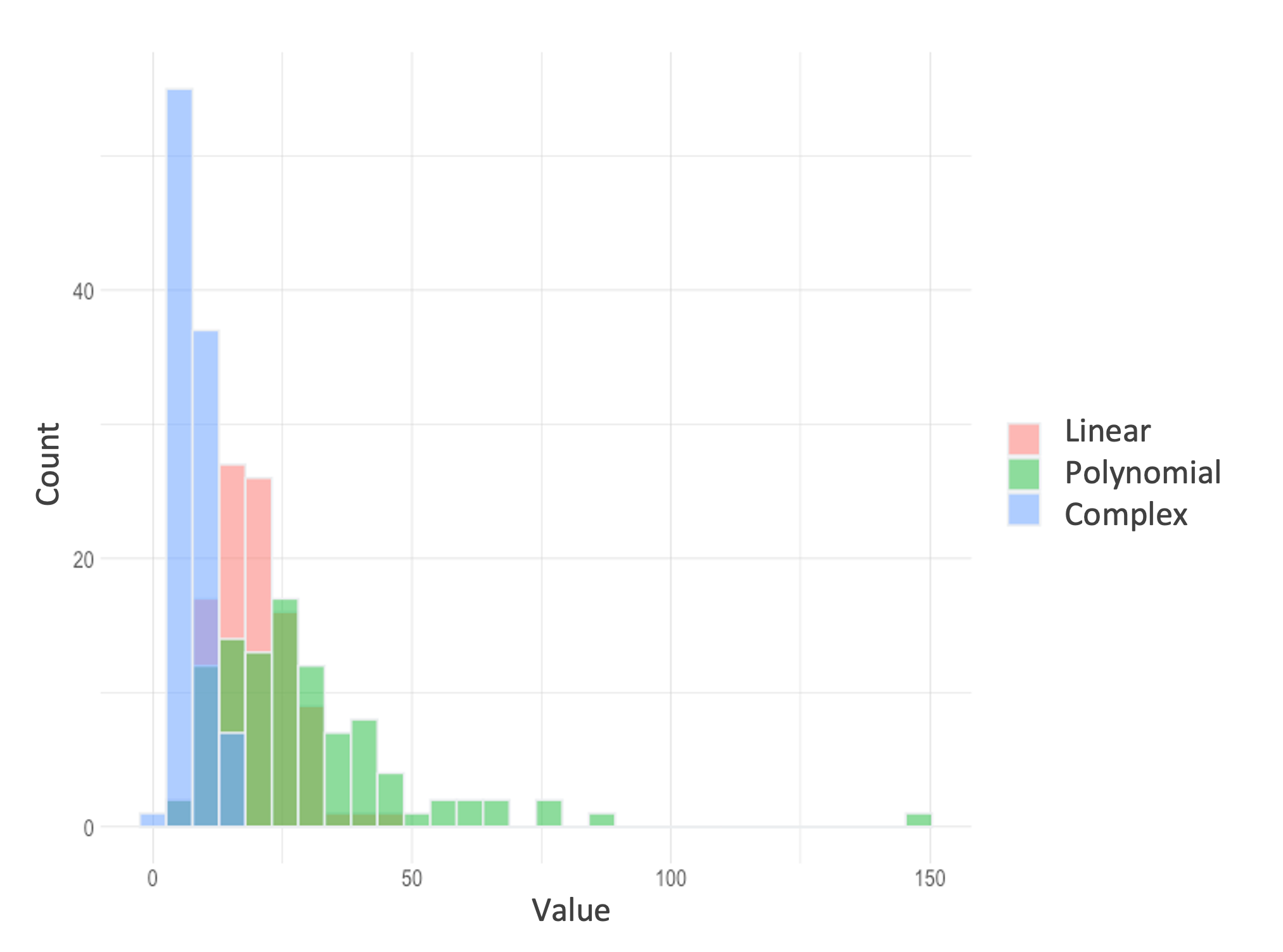
Figure 5: Histogram of the response variable in simulated datasets. Distribution of the response variable encompasses the relationship and joint distributional properties of each dataset. The proposed algorithm builds CI for each case, independent from their parametric distributional attributes. The polynomial dataset in particular has a long tail, resulting in a more challenging prediction task.

Table 1: The probability of true coverage and average CI half-width are calculated over 100 replications. The best coverage and half-width in each experiment are shown in bold.

					Regression Type	Linear		Polynomial		Complex
	Budget					Level of noise
Output Analysis Method	Total	$B_{1}$	$R$	$B_{2}$	Performance	low	high	low	high	low	high
Opt. Bias-corrected (VR)	1000	50	5	4	Coverage %	100	100	40	27	93	95
					Half-Width	0.6	2.8	1.0	10.7	0.8	6.0
Bias-corrected (VR)	1000	10	10	10	Coverage %	93	93	33	27	90	93
					Half-Width	0.6	5.3	1.5	13.7	0.7	6.2
Bias-corrected	1000	10	10	10	Coverage %	83	83	33	10	30	90
					Half-Width	0.7	6.0	1.7	15.6	0.8	7.5
IU-inflated Barton	1000	100	10	-	Coverage %	70	70	36	10	40	20
					Half-Width	0.3	2.3	1.0	9.2	0.6	5.4
IU-inflated Lam-Qian	1000	100	10	-	Coverage %	100	10	0	0	0	0
					Half-Width	2.4	7.2	2.6	7.9	2.5	7.7
LOOBoot	1000	100	10	-	Coverage %	15	0	0	0	5	2
					Hlaf-Width	0.6	1.8	19.4	19.9	0.6	2.7
Repeated cross-validation	1000	100	10	-	Coverage %	10	5	0	0	2	3
					Half-Width	0.3	1.3	7.2	7.7	0.4	1.4

The results indicate that the bias-corrected and variance-reduced (shown with “(VR)” in the table) confidence interval outperforms the other methods significantly. In complex and linear functions, Lam and Qian’s CI and Barton’s CI demonstrate relatively better performance compared to repeated cross-validation and LOOBoot. Furthermore, by employing optimized budget allocation, we can enhance the coverage probability, while reducing the CI’s half width. It should be noted that the half width of our proposed confidence intervals is comparable to that of Barton’s. This similarity stems from the fact that our variance estimators are computed in a similar manner, with a slight increase in variance due to the inclusion of multi-layer bias estimation in our confidence interval. Interestingly, repeated cross-validation yields the smallest half widths among all methods, leading to a near-zero probability of coverage.

7 Concluding Remarks

This paper showed the significance of incorporating bias and variance estimation in the model output analysis. We emphasize this matter via two common practical problems of machine learning and stochastic simulation. We bridge between the two fields providing a new playground for future research in the interconnection of ML and simulation.

We focused on non-parametric estimation methods to keep our results generalizable to data-driven problems. Furthermore, we addressed the computation inefficiency of non-parametric methods with an optimal budget allocation, which facilitates us to keep the computing budget the same while estimating the bias and variance of the model output. However, we do not include the model building cost in our computation budget, which can potentially be a drawback if a more complex model is fit. This problem can be addressed by restricting the non-parametric assumption to replace the bias estimator with a less number of resampling (Lin et al. 2015), which we leave for future research.

For both simulation and ML, our proposed method can be especially beneficial for big data problems, when due to computational expenses, the user can take smaller subsets of data for scalability. Leveraging the proposed bias-corrected CI can compensate for the loss of data.

Viewing ML as a simulation clarifies the propagation of bias of data into output. Without prediction bias, the estimates of future outcomes of a decision can mislead the decision-maker into choosing a worse and riskier option. One of the future research paths of interest would be incorporating the proposed estimator into data-driven optimization problems. The preliminary results of this paper was submitted to WSC 2021 (Vahdat and Shashaani 2021). The authors are also thankful to the AAUW Research Publication Grant in Engineering, Medicine and Science, American Educational Research Association that partially funded this project.

8 Theorem Proofs

8.1 Proof of Theorem 4.4

Proof 8.1

proof: Recall that $\hat{W}_{r}(\hat{F}^{*}_{b_{1}})=\bar{\Delta}^{*}_{r}\left(\hat{F}^{**}_{b_{1},.}\right)+\hat{\gamma}_{r}\left(\hat{F}^{**}_{b_{1},.}\right)$. Assume $\text{Var}\left(W_{r}(\hat{F}^{*}_{b_{1}})\right)<\infty.$ By the central limit theorem (More in-depth discussion on asymptotic behavior and validity of CLT in optimization space can be found in Hunter and Pasupathy (2022).) and definition of $\hat{W}_{r}(\hat{F}^{*}_{b_{1}})$, as $B_{2}$ grows larger, $\hat{W}_{r}(\hat{F}^{*}_{b_{1}})$ converges in distribution to Normal distribution with mean $W_{r}(\hat{F}^{*}_{b_{1}}),$ and variance $\text{Var}\left(W_{r}(\hat{F}^{*}_{b_{1}})\right).$ Moreover, the summation of $l$ squared standard independent Normal variables has Chi-squared distribution with $l$ degrees of freedom. Hence

$$\sum_{b_{2}=1}^{B_{2}}\left(\Delta^{*}_{r}(\hat{F}^{**}_{b_{1},b_{2}})+\hat{\gamma}_{r}(\hat{F}^{**}_{b_{1},b_{2}})-\hat{W}_{r}(\hat{F}^{*}_{b_{1}})\right)^{2}\sim\chi^{2}(B_{2}-1),$$

and $T$ follows student’s t distribution with $B_{2}-1$ degrees of freedom.

To show the validity of the proposed confidence intervals, note that for some $\alpha\in(0,1)$ and as $B_{2}\to\infty$

$$\mathbb{P}\Bigg{\{}-t_{B_{2}-1,\alpha/2}\leq\frac{\bar{\Delta}_{r}^{*}(\hat{F}^{**}_{b_{1},.})+\hat{\gamma}_{r}(\hat{F}^{**}_{b_{1},.})-W_{r}(\hat{F}^{*}_{b_{1}})}{\sqrt{\frac{1}{B_{2}-1}\sum_{b_{2}=1}^{B_{2}}\left(\Delta^{*}_{r}(\hat{F}^{**}_{b_{1},b_{2}})+\hat{\gamma}_{r}(\hat{F}^{**}_{b_{1},b_{2}})-\hat{W}_{r}(\hat{F}^{*}_{b_{1}})\right)^{2}}}\leq t_{B_{2}-1,\alpha/2}\Bigg{\}}=1-\alpha,$$

$$\implies \mathbb{P}\Bigg{\{}-t_{B_{2}-1,\alpha/2}\sqrt{\frac{1}{B_{2}-1}\sum_{b_{2}=1}^{B_{2}}\left(\Delta^{*}_{r}(\hat{F}^{**}_{b_{1},b_{2}})+\hat{\gamma}_{r}(\hat{F}^{**}_{b_{1},b_{2}})-\hat{W}_{r}(\hat{F}^{*}_{b_{1}})\right)^{2}}\leq$$

$$\ \ \ \ \ \bar{\Delta}_{r}^{*}(\hat{F}^{**}_{b_{1},.})+\hat{\gamma}_{r}(\hat{F}^{**}_{b_{1},.})-W_{r}(\hat{F}^{*}_{b_{1}})\leq$$

$$\ \ \ \ \ t_{B_{2}-1,\alpha/2}\sqrt{\frac{1}{B_{2}-1}\sum_{b_{2}=1}^{B_{2}}\left(\Delta^{*}_{r}(\hat{F}^{**}_{b_{1},b_{2}})+\hat{\gamma}_{r}(\hat{F}^{**}_{b_{1},b_{2}})-\hat{W}_{r}(\hat{F}^{*}_{b_{1}})\right)^{2}}\Bigg{\}}=1-\alpha$$

$$\implies \mathbb{P}\left\{T_{\text{min}}(\alpha)\leq W_{r}(\hat{F}^{*}_{b_{1}})\leq T_{\text{max}}(\alpha)\right\}=1-\alpha.$$

8.2 Proof of Theorem 4.6.

Proof 8.2

Proof. We first begin by deriving the (19) and (20), then show that given these definitions, the $\widehat{\text{IF}}_{2}\left(D_{i},D_{j};\hat{F}\right)$ is conditionally unbiased.

$$\frac{2}{\lambda} =\frac{m(m-1)(m-2)(m-3)}{m^{4}n^{2}}+\frac{m(m-1)(m-2)}{m^{3}n^{3}}\left(\frac{5n}{m}-4n\right)$$

$$\ \ \ +\frac{m(m-1)}{n^{2}m^{2}}\left(\frac{4}{m^{2}}+\frac{8}{mn}-\frac{8}{mn^{2}}+6\right)-\frac{4}{mn^{3}}-\frac{3}{n^{2}}-\frac{2}{m^{3}n}+\frac{5}{mn^{2}},$$

$$=\frac{10}{mn^{2}}-\frac{8}{m^{2}n^{2}}+\frac{4}{mn^{3}}-\frac{8}{mn^{4}}-\frac{8}{m^{2}n^{3}}+\frac{8}{m^{2}n^{4}}-\frac{2}{m^{3}n}=\frac{10}{mn^{2}}+\mathcal{O}\left(n^{-4}\right).$$

Hence $\lambda\approx-1/5\text{Cov}\left(N_{b_{1},i}/m,N_{b_{1},j}/m\right)$ and

$$\eta =\frac{m(m-1)(m-2)}{m^{3}n^{2}}+\frac{m(m-1)}{m^{3}n^{2}}\left(\frac{2}{m}-3\right)+\frac{2}{mn^{3}}+\frac{4-n}{n^{3}}$$

$$=\frac{7}{m^{2}n^{2}}-\frac{6}{mn^{2}}-\frac{2}{m^{3}n^{2}}+\frac{2}{mn^{3}}+\frac{4}{n^{3}}=-\frac{6}{mn^{2}}+\frac{4}{n^{3}}+\mathcal{O}(n^{-4}),$$

that can be simplified to $\eta\approx 6\text{Cov}(N_{b_{1},i}/m,N_{b_{1},j}/m)+4\mathbb{E}[N_{b_{1},i}/m]^{3}$.

Next, we need to show that the conditional expectation of the second order IF estimator given the empirical distribution is unbiased, i.e.,

$$\mathbb{E}_{Y}\left[\widehat{\text{IF}}_{2}\left(D_{i},D_{j};\hat{F}\right)|\hat{F}\right] =\mathbb{E}_{Y}\left[\frac{1}{B_{1}}\sum_{b_{1}=1}^{B_{1}}\frac{1}{R}\sum_{r=1}^{R}Y^{d}_{r}\left(\hat{F}^{*}_{b_{1}}\right)S^{(2)}_{i,j}\left(\hat{F}^{*}_{b_{1}}\right)+\frac{\lambda Y^{d}_{r}(\hat{F})}{mn^{2}}-\lambda\eta\widehat{\text{IF}}_{1}\left(D_{i};\hat{F}\right)\right]$$

$$=\frac{1}{B_{1}}\sum_{b_{1}=1}^{B_{1}}\frac{1}{R}\sum_{r=1}^{R}\mathbb{E}_{Y}\left[Y^{d}_{r}\left(\hat{F}^{*}_{b_{1}}\right)S^{(2)}_{i,j}\left(\hat{F}^{*}_{b_{1}}\right)+\frac{\lambda Y^{d}_{r}(\hat{F})}{mn^{2}}\right]-\mathbb{E}_{Y}\left[\lambda\eta\widehat{\text{IF}}_{1}\left(D_{i};\hat{F}\right)\right]$$

By substituting the $S^{(2)}_{i,j}\left(\hat{F}^{*}_{b_{1}}\right)$ according to its definition, the above equation becomes equivalent to

$$\mathbb{E}\Bigg{[}Y^{d}_{r}(\hat{F})\lambda\left(\frac{N_{b_{1},i}}{m}-\frac{1}{n}\right)\left(\frac{N_{b_{1},j}}{m}-\frac{1}{n}\right)+\sum_{i^{\prime}=1}^{n}\nabla_{\hat{F}}\theta(z_{i^{\prime}})\left(\frac{N_{i^{\prime}}}{m}-\frac{1}{n}\right)\lambda\left(\frac{N_{b_{1},i}}{m}-\frac{1}{n}\right)\left(\frac{N_{b_{1},j}}{m}-\frac{1}{n}\right)$$

$$+\frac{1}{2}\sum_{i^{\prime}=1}^{n}\sum_{j^{\prime}=1}^{n}\nabla^{2}_{\hat{F}}\theta(z_{i^{\prime}},z_{j^{\prime}})\left(\frac{N_{i^{\prime}}}{m}-\frac{1}{n}\right)\left(\frac{N_{j^{\prime}}}{m}-\frac{1}{n}\right)\lambda\left(\frac{N_{b_{1},i}}{m}-\frac{1}{n}\right)\left(\frac{N_{b_{1},j}}{m}-\frac{1}{n}\right)\Bigg{]}+\frac{\lambda Y^{d}_{r}(\hat{F})}{mn^{2}}-\lambda\eta\nabla_{\hat{F}}\theta$$

$$=\lambda Y^{d}_{r}(\hat{F})\text{Cov}\left(\frac{N_{i}}{m},\frac{N_{j}}{m}\right)+\nabla_{\hat{F}}\theta\lambda\mathbb{E}\left[\sum_{i^{\prime}=1}^{n}\left(\frac{N_{i^{\prime}}}{m}-\frac{1}{n}\right)\left(\frac{N_{b_{1},i}}{m}-\frac{1}{n}\right)\left(\frac{N_{b_{1},j}}{m}-\frac{1}{n}\right)\right]$$

$$\ \ \ +\frac{1}{2}\nabla^{2}_{\hat{F}}\theta\lambda\mathbb{E}\left[\sum_{i^{\prime}=1}^{n}\sum_{j^{\prime}=1}^{n}\left(\frac{N_{i^{\prime}}}{m}-\frac{1}{n}\right)\left(\frac{N_{j^{\prime}}}{m}-\frac{1}{n}\right)\left(\frac{N_{b_{1},i}}{m}-\frac{1}{n}\right)\left(\frac{N_{b_{1},j}}{m}-\frac{1}{n}\right)\right]+\frac{\lambda Y^{d}_{r}(\hat{F})}{mn^{2}}-\lambda\eta\nabla_{\hat{F}}\theta.$$

Exploiting the distributional properties of $N_{i},$ and knowing its higher order moments, allows us to further simplify the above expression to

$$\lambda Y^{d}_{r}(\hat{F})(\frac{-1}{mn^{2}})+\lambda\nabla_{\hat{F}}\theta\left(\frac{m(m-1)(m-2)}{m^{3}n^{2}}+\frac{m(m-1)}{m^{3}n^{2}}\left(\frac{2}{m}-3\right)+\frac{2}{mn^{3}}+\frac{4-n}{n^{3}}\right)$$

$$\ \ \ +\frac{1}{2}\nabla^{2}_{\hat{F}}\theta\lambda\Bigg{(}\frac{m(m-1)(m-2)(m-3)}{m^{4}n^{2}}+\frac{m(m-1)(m-2)}{m^{3}n^{3}}\left(\frac{5n}{m}-4n\right)$$

$$\ \ \ +\frac{m(m-1)}{n^{2}m^{2}}\left(\frac{4}{m^{2}}+\frac{8}{mn}-\frac{8}{mn^{2}}+6\right)-\frac{4}{mn^{3}}-\frac{3}{n^{2}}-\frac{2}{m^{3}n}+\frac{5}{mn^{2}}\Bigg{)}+\frac{\lambda Y^{d}_{r}(\hat{F})}{mn^{2}}-\lambda\eta\nabla_{\hat{F}}\theta.$$

By replacing the $\lambda$ with (19) and $\eta$ with, we get,

$$\mathbb{E}\left[\widehat{\text{IF}}_{2}\left(D_{i},D_{j};\hat{F}\right)|\hat{F}\right]=\frac{1}{2}\lambda\nabla^{2}_{\hat{F}}\theta(D_{i},D_{j})\frac{2}{\lambda}=\nabla^{2}_{\hat{F}}\theta(D_{i},D_{j}).$$

As per initial assumptions $\theta(.)$ is a smooth function of input distribution, therefore $\nabla\theta(.)$ is respectively a smooth function of the input distribution. Given $\nabla_{\hat{F}}^{2}\theta(.)<\infty$, we can apply the delta method and Glivenko-Cantelli theorem (Loève 1977) and achieve,

$$\mathbb{P}\left\{\lim_{n\to\infty}\sup_{D_{i},D_{j}}\bigg{|}\nabla^{2}_{\hat{F}}\theta(D_{i},D_{j})-\nabla^{2}_{F}\theta(D_{i},D_{j})\bigg{|}=0\right\}=1.$$

8.3 Proof of Lemma 4.7.

Proof 8.3

Proof. We take advantage of Covariance additivity property to calculate the covariance between $\widehat{\text{IF}}_{2}(\hat{F})$ and $\widehat{\text{IF}}_{1}(\hat{F})$.

$$\text{Cov}_{*}\left(\widehat{\text{IF}}_{2}(\hat{F}),\widehat{\text{IF}}_{1}(\hat{F})\right) =\text{Cov}_{*}\left(\bar{Y}(\hat{F})S_{i,j}+\frac{\lambda}{mn^{2}}-\lambda\eta\bar{Y}(\hat{F})S_{i},\bar{Y}(\hat{F})S_{i}\right)$$

$$=\text{Cov}_{*}\left(\bar{Y}(\hat{F})S_{i,j},\bar{Y}(\hat{F})S_{i}\right)+\frac{\lambda}{mn^{2}}\text{Cov}_{*}\left(Y(\hat{F}),\bar{Y}(\hat{F})S_{i}\right)$$

$$\ \ \ -\lambda\eta\text{Cov}_{*}\left(\bar{Y}(\hat{F})S_{i},\bar{Y}(\hat{F})S_{i}\right)$$

$$=\bar{Y}(\hat{F})^{2}(mn\lambda)\text{Cov}\left(\left(\frac{N_{i}}{m}-\frac{1}{n}\right)\left(\frac{N_{j}}{m}-\frac{1}{n}\right),\left(\frac{N_{i}}{m}-\frac{1}{n}\right)\right)-\lambda\eta\text{Var}\left(\bar{Y}(\hat{F})S_{i}\right)$$

$$=\bar{Y}(\hat{F})^{2}(mn\lambda)\Bigg{(}\mathbb{E}\left[(\frac{N_{i}}{m}-\frac{1}{n})^{2}(\frac{N_{j}}{m}-\frac{1}{n})\right]$$

$$\ \ \ -\mathbb{E}\left[(\frac{N_{i}}{m}-\frac{1}{n})(\frac{N_{j}}{m}-\frac{1}{n})\right]\mathbb{E}\left[(\frac{N_{i}}{m}-\frac{1}{n})\right]\Bigg{)}-\bar{Y}(\hat{F})^{2}\lambda\eta\text{Var}\left(\frac{N_{i}}{m}-\frac{1}{n}\right).$$

Now, given that the distribution of $N_{i}$ is known, we can simplify the above to,

$$\text{Cov}_{*}\left(\widehat{\text{IF}}_{2}(\hat{F}),\widehat{\text{IF}}_{1}(\hat{F})\right) =\frac{\bar{Y}(\hat{F})^{2}mn(mn^{2})}{5}\left(\frac{1}{mn}\left(\frac{2}{mn^{2}}+\frac{1}{n}-\frac{1}{mn}+1\right)\right)$$

$$\ \ \ -\frac{\bar{Y}(\hat{F})^{2}mn^{2}}{5}\left(\frac{-6}{mn^{2}}+\frac{4}{n^{3}}\right)\left(\frac{1}{mn}-\frac{1}{mn^{2}}\right)$$

$$=\frac{\bar{Y}(\hat{F})^{2}}{5}\left(2+mn-n+mn^{2}+\frac{6}{mn}-\frac{6}{mn^{2}}-\frac{4}{n^{2}}+\frac{4}{n^{3}}\right).$$

8.4 Proof of Theorem 4.9.

Proof 8.4

proof: The unbiased property follows directly from Lemmas 4.3 and  4.5 and Theorem 4.6. The debiased estimator can be expanded as the difference of the simulation output and the bias terms, i.e.,

$$\mathbb{E}[Y(\hat{F}^{*})-\hat{\beta}(\hat{F})-\hat{W}^{\text{cv}}(\hat{F}^{*})] =\mathbb{E}[Y(\hat{F}^{*})-\beta(\hat{F})-W(\hat{F}^{*})]+\mathbb{E}[\beta(\hat{F})-\hat{\beta}(\hat{F})]+\mathbb{E}[W(\hat{F}^{*})-\hat{W}^{\text{cv}}(\hat{F}^{*})]$$

$$=\theta(F_{0})+\mathcal{O}(\frac{1}{n^{3}})+\mathcal{O}(\frac{1}{\sqrt{B_{1}R}})+\mathcal{O}(\frac{1}{B_{2}})+\mathcal{O}(\frac{1}{R}).$$

The last equality is a direct derivation of (4) and unbiased properties of two bias estimators.

8.5 Proof of Theorem 4.10.

Proof 8.5

proof: Assume $\text{Var}\left(Y^{d}_{r}(\hat{F}^{*}_{b_{1}})\right)<\infty.$ Similar to the proof of Theorem 4.4, by the law of large numbers and the central limit theorem, as $R\times B_{1}$ grows larger, $\bar{Y}^{d}(\hat{F}^{*})$ converges to Normal distribution and subsequently,

$$\frac{\bar{Y}^{d}(\hat{F}^{*})-\theta(F_{0})}{\sqrt{\widehat{\text{Var}}\left(\bar{Y}^{d}(\hat{F}^{*})\right)/(RB_{1}-1)}}$$

converges to student’s t distribution with $RB_{1}-1$ degrees of freedom.

To show the validity of the proposed confidence intervals, note that for some $\alpha\in(0,1)$ and as $RB_{1}\to\infty$

$$\mathbb{P}\Bigg{\{}-t_{RB_{1}-1,\alpha/2}\leq\frac{\bar{Y}^{d}(\hat{F}^{*})-\theta(F_{0})}{\sqrt{\widehat{\text{Var}}\left(\bar{Y}^{d}(\hat{F}^{*})\right)/(RB_{1}-1)}}\leq t_{RB_{1}-1,\alpha/2}\Bigg{\}}=1-\alpha,$$

$$\implies \mathbb{P}\Bigg{\{}-t_{RB_{1}-1,\alpha/2}\sqrt{\widehat{\text{Var}}\left(\bar{Y}^{d}(\hat{F}^{*})\right)/(RB_{1}-1)}\leq\bar{Y}^{d}(\hat{F}^{*})-\theta(F_{0})\leq t_{RB_{1}-1,\alpha/2}\sqrt{\widehat{\text{Var}}\left(\bar{Y}^{d}(\hat{F}^{*})\right)/(RB_{1}-1)}\Bigg{\}}=1-\alpha$$

$$\implies \mathbb{P}\left\{L_{\text{min}}(\alpha)\leq\theta(F_{0})\leq L_{\text{max}}(\alpha)\right\}=1-\alpha.$$

8.6 Proof of Theorem 4.11.

Proof 8.6

Proof. Using the law of total variance we have,

$$\text{Var}\left(\hat{W}_{r}(\hat{F}^{*}_{b_{1}})\right) =\text{Var}\left(\frac{1}{B_{2}}\sum_{b_{2}=1}^{B_{2}}Y_{r}\left(\hat{F}^{**}_{b_{1},b_{2}}\right)-\frac{1}{B_{2}}\sum_{b_{2}=1}^{B_{2}}Y_{r}\left(\hat{F}^{***}_{b_{1},b_{2}}\right)\right)$$

$$=\text{Var}\left(\frac{1}{B_{2}}\sum_{b_{2}=1}^{B_{2}}Y_{r}\left(\hat{F}^{**}_{b_{1},b_{2}}\right)\right)+\text{Var}\left(\frac{1}{B_{2}}\sum_{b_{2}=1}^{B_{2}}Y_{r}\left(\hat{F}^{***}_{b_{1},b_{2}}\right)\right)$$

$$-2\text{Cov}\left(\frac{1}{B_{2}}\sum_{b_{2}=1}^{B_{2}}Y_{r}\left(\hat{F}^{**}_{b_{1},b_{2}}\right),\frac{1}{B_{2}}\sum_{b_{2}=1}^{B_{2}}Y_{r}\left(\hat{F}^{***}_{b_{1},b_{2}}\right)\right)$$

$$=\frac{\text{Var}\left(Y_{r}\left(\hat{F}^{**}_{b_{1},b_{2}}\right)\right)}{B_{2}}+\frac{B_{2}-1}{B_{2}}\text{Cov}\left(Y_{r}\left(\hat{F}^{**}_{b_{1},b_{2}}\right),Y_{r}\left(\hat{F}^{**}_{b_{1},b^{\prime}_{2}}\right)\right)$$

$$+\frac{\text{Var}\left(Y_{r}\left(\hat{F}^{***}_{b_{1},b_{2}}\right)\right)}{B_{2}}+\frac{B_{2}-1}{B_{2}}\text{Cov}\left(Y_{r}\left(\hat{F}^{***}_{b_{1},b_{2}}\right),Y_{r}\left(\hat{F}^{***}_{b_{1},b^{\prime}_{2}}\right)\right)$$

$$-\frac{2}{B_{2}^{2}}B_{2}^{2}\text{Cov}\left(Y_{r}\left(\hat{F}^{**}_{b_{1},b_{2}}\right),Y_{r}\left(\hat{F}^{***}_{b_{1},b_{2}}\right)\right).$$

As proved in DeGroot (1989), the variance and covariance between averages of bootstrap samples can be calculated as a function of the variance of the random variable, which for our case is, for a given $r$, $\text{Var}\left(Y_{r}(\hat{F}^{*}_{b_{1}})\right)$. Since we are looking at the conditional variance, $\text{Var}\left(Y_{r}(\hat{F}^{*}_{b_{1}})\right)$ is no longer random (for brevity we refer to $\text{Var}\left(Y_{r}(\hat{F}^{*}_{b_{1}})\right)$ as $\sigma^{2}$). Therefore,

$$\text{Var}\left(\hat{W}_{r}(\hat{F}^{*}_{b_{1}})\right) =\frac{\sigma^{2}(2m^{*}-1)}{B_{2}(m^{*})^{2}}\left(1+\frac{1}{B_{2}}\right)+\frac{(B_{2}-1)\sigma^{2}}{B_{2}m^{*}}\left(1+\frac{B_{2}-1}{B_{2}}\right)-2\frac{\sigma^{2}}{m^{*}}.$$

Setting the variance of the bias to be in the order of $\Theta\left(\text{Var}\left(Y\left(\hat{F}^{*}_{b_{1}}\right)\right)/(m^{*})^{3}\right)$ results in

$$B_{2}^{*}=\Theta\left(\left(\frac{3(m^{*})^{2}-m^{*}}{m^{*}+1}\right)^{1/3}\right).$$

References

- Ankenman and Nelson (2012) Ankenman BE, Nelson BL (2012) A quick assessment of input uncertainty. Proceedings of the 2012 Winter Simulation Conference (WSC), 1–10 (IEEE).
- Austin and Tu (2004) Austin PC, Tu JV (2004) Bootstrap methods for developing predictive models. The American Statistician 58(2):131–137, URL http://dx.doi.org/10.1198/0003130043277.
- Barton (2012) Barton RR (2012) Tutorial: Input uncertainty in output analysis. Proceedings of the 2012 Winter Simulation Conference (WSC), 1–12 (IEEE).
- Barton et al. (2018) Barton RR, Lam H, Song E (2018) Revisiting direct bootstrap resampling for input model uncertainty. 2018 Winter Simulation Conference (WSC), 1635–1645 (IEEE).
- Barton et al. (2022) Barton RR, Lam H, Song E (2022) Input uncertainty in stochastic simulation. The Palgrave Handbook of Operations Research, 573–620 (Springer).
- Barton and Schruben (1993) Barton RR, Schruben LW (1993) Uniform and bootstrap resampling of empirical distributions. Proceedings of the 25th conference on Winter simulation, 503–508.
- Barton and Schruben (2001) Barton RR, Schruben LW (2001) Resampling methods for input modeling. Proceedings of the 33nd Conference on Winter Simulation, 372–378 (IEEE Computer Society).
- Blanchet and Glynn (2015) Blanchet JH, Glynn PW (2015) Unbiased monte carlo for optimization and functions of expectations via multi-level randomization. 2015 Winter Simulation Conference (WSC), 3656–3667, URL http://dx.doi.org/10.1109/WSC.2015.7408524, ISSN: 1558-4305.
- Breiman (2001) Breiman L (2001) Random forests. Machine learning 45(1):5–32.
- Chang and Hall (2015) Chang J, Hall P (2015) Double-bootstrap methods that use a single double-bootstrap simulation. Biometrika 102(1):203–214, ISSN 00063444, 14643510, URL http://www.jstor.org/stable/43305647.
- Cheng and Holloand (1997) Cheng RCH, Holloand W (1997) Sensitivity of computer simulation experiments to errors in input data. Journal of Statistical Computation and Simulation 57(1-4):219–241, URL http://dx.doi.org/10.1080/00949659708811809.
- Davison and Hinkley (1997) Davison AC, Hinkley DV (1997) Bootstrap Methods and their Application. Cambridge Series in Statistical and Probabilistic Mathematics (Cambridge University Press).
- DeGroot (1989) DeGroot MH (1989) Probability and Statistics (Addison-Wesley Pub. Co.).
- Efron (1979) Efron B (1979) Bootstrap methods: Another look at the jackknife. The Annals of Statistics 7(1):1–26, ISSN 00905364, URL http://www.jstor.org/stable/2958830.
- Efron (1983) Efron B (1983) Estimating the error rate of a prediction rule: Improvement on cross-validation. Journal of the American Statistical Association 78(382):316–331, ISSN 01621459, URL http://www.jstor.org/stable/2288636.
- Efron (2014) Efron B (2014) Estimation and accuracy after model selection. Journal of the American Statistical Association 109(507):991–1007, URL http://dx.doi.org/10.1080/01621459.2013.823775.
- Efron (2020) Efron B (2020) Prediction, estimation, and attribution. Journal of the American Statistical Association 115(530):636–655.
- Efron and Tibshirani (1997) Efron B, Tibshirani R (1997) Improvements on cross-validation: The .632+ bootstrap method. Journal of the American Statistical Association 92(438):548–560, ISSN 01621459.
- Fithian et al. (2014) Fithian W, Sun D, Taylor J (2014) Optimal inference after model selection. arXiv preprint arXiv:1410.2597 .
- Geisser (1975) Geisser S (1975) The predictive sample reuse method with applications. Journal of the American statistical Association 70(350):320–328.
- Ghosh et al. (2018) Ghosh S, Squillante M, Wollega E (2018) Efficient stochastic gradient descent for learning with distributionally robust optimization. arXiv preprint arXiv:1805.08728 .
- Giles (2008) Giles MB (2008) Multilevel monte carlo path simulation. Operations research 56(3):607–617.
- Glasserman (2004) Glasserman P (2004) Monte Carlo methods in financial engineering, volume 53 (Springer).
- Hall (1986) Hall P (1986) On the Bootstrap and Confidence Intervals. The Annals of Statistics 14(4):1431 – 1452, URL http://dx.doi.org/10.1214/aos/1176350168.
- Hunter and Pasupathy (2022) Hunter SR, Pasupathy R (2022) Central limit theorems for constructing confidence regions in strictly convex multi-objective simulation optimization. 2022 Winter Simulation Conference (WSC), 3015–3026 (IEEE).
- Iyengar et al. (2023) Iyengar G, Lam H, Wang T (2023) Optimizer’s information criterion: Dissecting and correcting bias in data-driven optimization. arXiv preprint arXiv:2306.10081 .
- Kleywegt et al. (2002) Kleywegt AJ, Shapiro A, Homem-de Mello T (2002) The sample average approximation method for stochastic discrete optimization. SIAM Journal on Optimization 12(2):479–502.
- Koenig and Law (1985) Koenig LW, Law AM (1985) A procedure for selecting a subset of size m containing the l best of k independent normal populations, with applications to simulation. Communications in Statistics - Simulation and Computation 14(3):719–734, URL http://dx.doi.org/10.1080/03610918508812467.
- Lam (2016) Lam H (2016) Advanced tutorial: Input uncertainty and robust analysis in stochastic simulation. 2016 Winter Simulation Conference (WSC), 178–192 (IEEE).
- Lam (2021) Lam H (2021) On the impossibility of statistically improving empirical optimization: A second-order stochastic dominance perspective. arXiv preprint arXiv:2105.13419 .
- Lam and Qian (2019) Lam H, Qian H (2019) Random perturbation and bagging to quantify input uncertainty. 2019 Winter Simulation Conference (WSC), 320–331, URL http://dx.doi.org/10.1109/WSC40007.2019.9004757.
- Lam and Qian (2021) Lam H, Qian H (2021) Subsampling to enhance efficiency in input uncertainty quantification. Operations Research opre.2021.2168, URL http://dx.doi.org/10.1287/opre.2021.2168.
- Lam and Zhang (2021) Lam H, Zhang J (2021) Distributionally constrained black-box stochastic gradient estimation and optimization. arXiv preprint arXiv:2105.09177 .
- Lin et al. (2015) Lin Y, Song E, Nelson BL (2015) Single-experiment input uncertainty. Journal of Simulation 9(3):249–259.
- Loève (1977) Loève M (1977) Elementary probability theory (Springer).
- Massart (1990) Massart P (1990) The tight constant in the dvoretzky-kiefer-wolfowitz inequality. The Annals of Probability 18(3):1269–1283.
- Montgomery (2009) Montgomery DC (2009) Design and Analysis of Experiments (John Wiley), 7th edition.
- Morgan et al. (2019) Morgan LE, Nelson BL, Titman AC, Worthington DJ (2019) Detecting bias due to input modelling in computer simulation. European Journal of Operational Research 279(3):869–881.
- Morgan et al. (2022) Morgan LE, Rhodes-Leader L, Barton RR (2022) Reducing and calibrating for input model bias in computer simulation. INFORMS Journal on Computing .
- Nelson (1990) Nelson BL (1990) Control variate remedies. Operations Research 38(6):974–992, URL http://dx.doi.org/10.1287/opre.38.6.974.
- Ouysse (2013) Ouysse R (2013) A fast iterated bootstrap procedure for approximating the small-sample bias. Communications in Statistics - Simulation and Computation 42(7):1472–1494, ISSN 0361-0918, 1532-4141, URL http://dx.doi.org/10.1080/03610918.2012.667473.
- Rabbi et al. (2021) Rabbi F, Khan S, Khalil A, Mashwani WK, Shafiq M, Göktaş P, Unvan Y (2021) Model selection in linear regression using paired bootstrap. Communications in Statistics - Theory and Methods 50(7):1629–1639, URL http://dx.doi.org/10.1080/03610926.2020.1725829.
- Raschka (2018) Raschka S (2018) Model evaluation, model selection, and algorithm selection in machine learning. arXiv e-prints URL https://arxiv.org/abs/1811.12808v3.
- Reichert and Schuwirth (2012) Reichert P, Schuwirth N (2012) Linking statistical bias description to multiobjective model calibration. Water Resources Research 48(9).
- Ross (2022) Ross SM (2022) Simulation (academic press).
- Shao (1996) Shao J (1996) Bootstrap model selection. Journal of the American Statistical Association 91(434):655–665, ISSN 01621459, URL http://www.jstor.org/stable/2291661.
- Shashaani and Vahdat (2022) Shashaani S, Vahdat K (2022) Improved feature selection with simulation optimization. Optimization and Engineering 1573–2924, URL http://dx.doi.org/https://doi.org/10.1007/s11081-022-09726-3.
- Song and Nelson (2019) Song E, Nelson BL (2019) Input–output uncertainty comparisons for discrete optimization via simulation. Operations Research 67(2):562–576.
- Stone (1974) Stone M (1974) Cross-validation and multinomial prediction. Biometrika 61(3):509–515.
- Sun et al. (2011) Sun Y, Apley DW, Staum J (2011) Efficient nested simulation for estimating the variance of a conditional expectation. Operations Research 59(4):998–1007.
- Vahdat and Shashaani (2021) Vahdat K, Shashaani S (2021) Non-parametric uncertainty bias and variance estimation via nested bootstrapping and influence functions. 2021 Winter Simulation Conference (WSC), 1–12, URL http://dx.doi.org/10.1109/WSC52266.2021.9715420.
- Van der Vaart (1998) Van der Vaart AW (1998) Asymptotic Statistics. Cambridge Series in Statistical and Probabilistic Mathematics (Cambridge University Press), URL http://dx.doi.org/10.1017/CBO9780511802256.
- Yang et al. (2021) Yang R, Kent D, Apley DW, Staum J, Ruppert D (2021) Bias-corrected estimation of the density of a conditional expectation in nested simulation problems. ACM Trans. Model. Comput. Simul. 31(4), ISSN 1049-3301, URL http://dx.doi.org/10.1145/3462201.