Disintegration of Gaussian Measures for Sequential Assimilation of Linear Operator Data

Abstract

Gaussian processes appear as building blocks in various stochastic models and have been found instrumental to account for imprecisely known, latent functions. It is often the case that such functions may be directly or indirectly evaluated, be it in static or in sequential settings. Here we focus on situations where, rather than pointwise evaluations, evaluations of prescribed linear operators at the function of interest are (sequentially) assimilated. While working with operator data is increasingly encountered in the practice of Gaussian process modelling, mathematical details of conditioning and model updating in such settings are typically by-passed. Here we address these questions by highlighting conditions under which Gaussian process modelling coincides with endowing separable Banach spaces of functions with Gaussian measures, and by leveraging existing results on the disintegration of such measures with respect to operator data. Using recent results on path properties of GPs and their connection to RKHS, we extend the Gaussian process - Gaussian measure correspondence beyond the standard setting of Gaussian random elements in the Banach space of continuous functions. Turning then to the sequential settings, we revisit update formulae in the Gaussian measure framework and establish equalities between final and intermediate posterior mean functions and covariance operators. The latter equalities appear as infinite-dimensional and discretization-independent analogues of Gaussian vector update formulae.

and

t1The authors gratefully acknowledge funding from the Swiss National Science Fundation (SNF) through project no. 178858.

1 Introduction

Gaussian process (GP) stochastic models have found broad use in a variety of domains such as filtering, geostatistics, or analysis of computer codes. They are also frequently used in machine learning as priors on functions for tasks where one tries to learn a unknown function $f$ in a Bayesian way. Such machine learning uses include, among others, Bayesian inversion [22] and Bayesian optimization [29, 32, 26].

One reason for the success of GPs in these domains is their closure under pointwise observations. Indeed, given a GP $Z=(Z_{s})_{s\in D}$ on some domain $D$ and a set of points $s_{1},...,s_{n}\in D$, the distribution of $Z$ conditionally on $Z_{s_{1}},...,Z_{s_{n}}$ is again Gaussian, with mean and covariance functions that can be computed in closed form, see e.g. [35].

While traditional machine learning tended to focus only on data in the form of pointwise evaluations, other types of indirect, functional data become increasingly available, such as tomographic data, or derivative data [42, 36] that do not boil down to simple pointwise evaluations of the original latent function. This has sparked interest in extending GPs to different types of observations, such as integral observations [20, 23] or linear constraints [25, 1]. Broadly speaking, these methods aim at learning $f$ from linear form data $\ell_{i}(f)$, where $\ell_{i}:X\rightarrow\mathbb{R}$ ($i=1,2,\dots$) are linear functionals on some Banach space $X$ of functions on $D$. Just like under pointwise observations, working out conditional distributions boils down to applying conditioning formulae to finite-dimensional vectors, in that case to vectors of the form $(Z_{s},Z_{s^{\prime}},\ell_{1}(Z),\dots,\ell_{n}(Z))$ ($s,s^{\prime}\in D$).

Compared to the basic case of pointwise observations, however, ensuring that the usual way of deriving conditional distributions does actually work under linear form data requires a bit of care. The usual approach in practice is to silently assume that the considered functionals of $Z$ can be expressed as limits of linear combinations of pointwise field evaluations, so that everything will work as intended. In several cases, this condition might not be straightforward to verify, and things can get even worse when one considers observations described by linear operators between Banach spaces $G:X\rightarrow Y$, thus raising the question of what kind of operator data can be assimilated, or more precisely, of which properties an operator $G$ needs to satisfy in order for the conditional law to be well-defined. While this question can be tricky to answer using the traditional Gaussian process framework, modern probability theory in Banach spaces offers a rigorous, generic approach to conditioning under linear operator using the language of disintegrations of measures, as we will clarify next.

Beyond establishing solid mathematical foundations for conditioning on linear operator data, another problem that has received much attention lately in the GP litterature is that of efficiently performing sequential data assimilation [3, 21, 43]. In such a framework, new data become available sequentially and predictions have to be recomputed along the way to incorporate the new information. To alleviate the computational burden associated to sequential learning, various updating scheme have been developed [11, 15, 18, 4] which aim at expressing the contribution of the new data as an update to the current posterior.

In the present work, we focus on the intersection of the two aforementioned topics, that is, we concentrate on sequential assimilation of linear operator data. Our aim is to provide an abstract mathematical foundation for the above setting by formulating it in the language of disintegrations and to derive update formulae for disintegrations. In passing, we clarify the link between the traditional Gaussian process framework and the Gaussian measure language. This work emerged as a theoretical foundation for practical approaches to large-scale assimilation of linear operator data under GP priors developed in [50].

The article is structured as follows: in Section 2, we review results from Rajput and Cambanis, [34] in order to prove equivalence of the Gaussian process and Gaussian measure approaches in various cases. We also connect this with recent results on sample path properties of GP [44] to characterize situations under which GPs induce a Gaussian measure on some suitable space of functions.

Then, in Section 3, we turn to disintegrations of Gaussian measures [49], which we extend to the non-centred and sequential case, thereby providing an extension of the usual kriging update formulae [11] to disintegrations.

Those results offer prospects for theoretical inquiries in Bayesian optimization [5] as well more applied uses, such as the formulation of discretization-independent algorithms in Bayesian inversion [12]. We also hope that our characterization of the Gaussian process - Gaussian measure equivalence will help bring benefits of the abstract language of disintegrations to the applied GP community.

Example.

For the rest of this work, we will consider the task of learning an unknown function $f$ living in a separable Banach space $X$ from data of the form $y_{i}=G_{i}(f),~{}i=1,\dotsc,n$, where

$$G_{i}:X\rightarrow Y,$$

are bounded liner operators into a separable Banach space $Y$, we will call the $G_{i}$ the observation operators. As a simple example of a problem falling into this setting, consider the task of learning a continuous function defined on the interval $\left[-1,1\right]$ via different types of data: pointwise function values, integrals of the function, Fourier coefficients, etc. Figure 1 provides an illustration of solutions obtained under a Gaussian process prior. Note that the three different combinations of observations in Figure 1 can each be described by a linear operator $G:C\left(\left[-1,1\right]\right)\rightarrow\mathbb{R}^{p}$

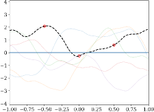
(a)

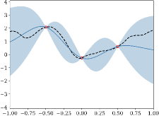
(b)

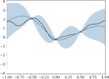
(c)

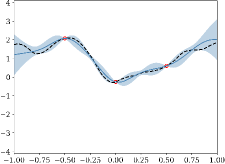
(d)

Figure 1: Conditional mean (blue) and 2$\sigma$ credible intervals after inclusion of different types of data: (a) realizations independently sampled from the prior GP, (b) prediction based on pointwise data at 3 locations, (c) prediction based on pointwise data + integral over domain, (d) prediction based on pointwise data + integral over domain + first two Fourier coefficients. The true unknown function is shown in dashed black.

Note that this example can already serve to illustrate the theoretical difficulties associated with the conditional law under linear operator observations. Consider for example derivative observations $y=f^{\prime}(x_{0}),~{}x_{0}\in D$. The usual procedure when working with derivatives of GPs is to assume mean square differentiability of the process. But even then, results on the link between mean square differentiability of the process and almost sure differentiability of the paths [10, 40] require additional assumptions to ensure path differentiability, so that the observation operator is not guaranteed to be bounded.

2 Gaussian Processes and Gaussian Measure: Background and Equivalence

When working with Gaussian priors over spaces of function defined over an arbitrary domain $D$, two complementary approaches are often used:

• One can work with a Gaussian process on $D$, which is defined as a stochastic process $Z=(Z_{s})_{s\in D}$ indexed by $D$, such that for any number of points $s_{1},...,s_{n}\in D$, the distribution of $\left(Z_{s_{1}},...,Z_{s_{n}}\right)$ is Gaussian, e.g., [48, 38].

• One can work with a Gaussian measure which is defined as a Borel measure on $C(D)$ such that for any continuous linear functional $\ell\in C(D)^{*}$, the measure $\ell_{\#}\mu=\mu\circ\ell^{-1}$ on $\mathbb{R}$ is Gaussian, e.g., [46, 13, 47, 16].

For a Gaussian process $Z$ as introduced above, its mean and covariance function are defined as

$$m:s\in D\mapsto m(s)=\mathbb{E}\left[Z_{x}\right]$$

$$k:(s,t)\in D^{2}\mapsto k(s,t)=\mathbb{E}\left[Z_{s}Z_{t}\right]-\mathbb{E}\left[Z_{s}\right]\mathbb{E}\left[Z_{t}\right],$$

where the existence of moments is guaranteed by the joint Gaussianity of $(Z_{s},Z_{t})$ for any $(s,t)\in D^{2}$. Note that here we will often used the alternative notation $m_{s}$ for $m(s)$ as it will increase the readability of forthcoming equations.

When working with a Gaussian measure $\mu$ over a separable Banach space $X$, the notions of mean and covariance functions are respectively replaced by the mean element and covariance operator. Here we denote by $X^{*}$ the (continuous) dual space of $X$, and for any element $f\in X$ and continuous linear form $g^{*}$ we use the duality notation $\langle f,g^{*}\rangle=g^{*}(f)$.

Definition 1.

Given a Gaussian measure $\mu$ on a Banach space $X$, the mean of $\mu$ is the unique element $m_{\mu}\in X$ such that:

$$\int_{X}\langle f,g^{*}\rangle d\mu(f)=\langle m_{\mu},g^{*}\rangle,~{}\forall g^{*}\in X^{*}.$$ (2.1)

The covariance operator of $\mu$ is the linear operator $C_{\mu}:X^{*}\rightarrow X$ defined by

$$\langle C_{\mu}g_{1}^{*},g_{2}^{*}\rangle=\int_{X}\left(\langle f,g_{1}^{*}\rangle-\langle m_{\mu},g_{1}^{*}\rangle\right)\left(\langle f,g_{2}^{*}\rangle-\langle m_{\mu},g_{2}^{*}\rangle\right)d\mu(f),~{}\forall g_{1}^{*},g_{2}^{*}\in X^{*}$$ (2.2)

We refer the reader to Vakhania et al., [51] for more details.

When considering Gaussian processes with continuous trajectories over a compact metric space $D$, the Gaussian process and Gaussian measure points of view are known to be equivalent, with $X$ being the Banach space of continuous functions $C(D)$ equipped with the sup norm. Indeed, one can show that a Gaussian measure on $C(D)$ defines an equivalent Gaussian process on D with continuous trajectories, and vice-versa. This allows one to work with Gaussian measures and Gaussian processes interchangeably on this Banach space. The equivalence is ensured by the following two theorems, which are multidimensional analogues of the one presented in Rajput and Cambanis, [34].

We first show that a Gaussian process on $D$ with continuous sample paths induces a Gaussian measure on $C(D)$. Indeed, given such a Gaussian process $Z$, one may try to induce a measure $\mu_{Z}:=\mathbb{P}\circ\Phi^{-1}$, where $\Phi:=Z\left(\cdot;\omega\right)$. The next theorem guarantees that this indeed defines a Gaussian measure. This result is well known in the Gaussian measure litterature (see e.g. [8]) and we provide a proof in the appendix for the sake of completeness.

Theorem 1.

Let $\left(\Omega,\mathcal{F},\mathbb{P};Z(\omega,s),s\in D\right)$ be a Gaussian process on a compact metric space $D$ with continuous sample paths. Then the induced measure

$$\mu_{Z}:=\mathbb{P}\circ\Phi^{-1}$$

is well-defined (as a Borel measure) and Gaussian.

On the other hand, given a Gaussian measure $\mu$ on $C(D)$, the following theorem ensures that $\mu$ induces indeed a Gaussian process.

Theorem 2.

Let $\mu$ be a Gaussian measure on $C(D)$, for a compact metric space $D$. Then, letting $\Omega=C(D)$ and $\mathcal{F}$ be the Borel sigma algebra on $C(D)$, the collection of random variables

$$Z_{s}:\left(\Omega,\mathcal{F},\mu\right)\rightarrow\left(\mathbb{R},\mathcal{B}\left(\mathbb{R}\right)\right),~{}\omega\mapsto\delta_{s}\left(\omega\right)$$

for all $s\in D$ defines a Gaussian process with paths in $C(D)$ which induces $\mu$ on $C(D)$.

Under this correspondence, the mean and covariance functions of the process may be obtained as special cases of the mean element and covariance operator of the corresponding measure by acting on them with Dirac delta functionals (which in this case belong to the continuous dual of the Banach space under consideration):

Lemma 1.

Let $Z$ be a Gaussian process on a compact metric space $D$ with continuous trajectories, and let $\mu$ be the corresponding induced measure on $C(D)$. Then the covariance operator and mean element of the measure are related to the mean and covariance function of the process via

$$m_{s} =\mathbb{E}\left[Z_{s}\right]=\langle m_{\mu},\delta_{s}\rangle,$$ (2.3)

$$k(s_{1},s_{2}) =\mathbb{E}\left[Z_{s_{1}}Z_{s_{2}}\right]-\mathbb{E}\left[Z_{s_{1}}\right]\mathbb{E}\left[Z_{s_{2}}\right]=\langle C_{\mu}\delta_{s_{2}},\delta_{s_{1}}\rangle,$$ (2.4)

for all $s_{1},s_{2}\in D$.

These considerations allow us to work interchangeably with the two points of views. While in many practical circumstances the GP point of view is sufficient, Gaussian measures can be leveraged to provide rigorous updating of GPs under linear operator observations, as we will show in Section 3.

Remark 1.

The correspondence between Gaussian processes and measures is not limited to the Banach space $C(D)$ of continuous functions over a compact metric space. Indeed Rajput and Cambanis, [34] also prove correspondence for $L^{p}$ spaces and spaces of absolutely continuous functions. However, the proofs are done on a case by case basis.

Even if the Banach space $C(D)$ of continuous functions on a compact domain provides a basic setting for the Gaussian process - Gaussian measure equivalence, it often proves insufficient when one wants to use this correspondence to tackle conditioning under linear operator observations. For example, the differential operator $d/dx$ is not even a well-defined operator on $C(D)$. For such operators, the natural domains to consider are Sobolev spaces. This shows that, in the Gaussian measure framework, when one wants to assimilate observations that are ”finer” than simple pointwise evaluations, one has to go beyond the Banach space $C(D)$. This is what we will do in the following section by considering reproducing kernel Hilbert spaces.

The Reproducing Kernel Hilbert Space Case: The proofs of the process-measure equivalence theorems Theorems 1 and 2 in the Banach space of continuous functions over a compact domain rely on having a characterization of the dual space of the Banach space under consideration, and on being able to approximate elements of the dual via pointwise evaluations. Indeed, Gaussian measures on a Banach space are characterized by the Gaussianity of their linear functionals, whereas GPs are characterized by the Gaussianity of finite collections of field evaluations, making the link between linear functionals and pointwise evaluations a crucial one in the correspondence.

The natural class of spaces where such a link exists is that of reproducing kernel Hilbert spaces (RKHS) [2, 41, 6, 27]. Indeed, one of the defining properties of RKHS is that their (continuous) dual contain the evaluation functionals, so that one can directly adapt the process-measure correspondence theorems. Note that the product measurability is still guaranteed by Theorem 10 since RKHS of functions over a compact metric space are contained in the Banach space of continuous functions provided that the reproducing kernel is continuous.

Theorem 3.

Let $\left(\Omega,\mathcal{F},\mathbb{P};Z(\omega,s),s\in D\right)$ be a Gaussian process with trajectories in a separable RKHS $\mathcal{H}$ of functions over a compact metric space $D$. Then the induced measure

$$\mu_{Z}:=\mathbb{P}\circ\Phi^{-1}$$

is well-defined (as a Borel measure) and Gaussian.

Theorem 4.

Let $\mu$ be a Gaussian measure on a separable RKHS $\mathcal{H}$ of functions over a compact metric space $D$. Then, letting $\Omega=\mathcal{H}$ and $\mathcal{F}$ be the Borel sigma algebra on $\mathcal{H}$, the collection of random variables

$$Z_{s}:\left(\Omega,\mathcal{F},\mu\right)\rightarrow\left(\mathbb{R},\mathcal{B}\left(\mathbb{R}\right)\right),~{}\omega\mapsto\delta_{s}\left(\omega\right)$$

for all $s\in D$ is a Gaussian process with paths in $\mathcal{H}$ which induces $\mu$ on $\mathcal{H}$.

The question of whether GP sample paths lie in an RKHS has been widely studied in the litterature [45, 44]. One of the most well-known results in this domain is a negative one, namely that for a GP with continuous covariance kernel and almost-sure sample paths, the probability that the trajectories lie within the RKHS associated to the kernel of the process is zero [14, 31]. Recent works have aimed at finding ”larger” RKHS that contain the paths of the process. It turns out that for a broad class of GPs, one can find an ’interpolating’ RKHS lying between the RKHS of the kernel of the process and $L^{2}(\nu)$ (for some measure $\nu$) that contains the sample paths almost surely [44, Corollary 5.3].

We here only consider kernels that are bounded on the diagonal: $k(s,s)<\infty,\text{ all }s\in D$ (as is the case for all the usual kernels). Then, Steinwart and Scovel, [45, Lemma 5.1, Theorem 5.3] guarantee that the conditions required for the sample paths to be contained in powers of the base RKHS hold. Under these conditions, there are results that guarantee the existence of an RKHS containing the trajectories of the process with probability $1$. The RKHS depends on the eigenvalues of the operator

$$T_{k}(f):=\int_{D}k(\cdot,s)f(s)d\nu(s),~{}f\in L_{2}(\nu),$$

where $\nu$ is any finite Borel measure supported on $D$. The embedding RKHS is then constructed as a power $\mathcal{H}_{k}^{\theta}$ of the RKHS $\mathcal{H}_{k}$ of the kernel [27, Definition 4.12].

Theorem 5.

[Kanagawa et al., [27, Theorem 4.12], Steinwart, [44, Theorem 5.2]] Let $Z$ be a Gaussian process over a compact domain $D\subset\mathbb{R}^{d}$ with covariance kernel $k$. Let also $\left(\lambda_{i},\phi_{i}\right)_{i\in\mathbb{N}}$ be the eigensystem of the operator $T_{k}$. Then, provided $\sum_{i\in\mathbb{N}}\lambda_{i}^{1-\theta}<\infty$, there exists a version of $Z$ whose sample paths lie in $\mathcal{H}_{k}^{\theta}$ with probability $1$.

In particular, for GPs with Gaussian kernels or Matérn kernels, one can always find an RKHS that contains the sample paths of the GP with probability $1$, as the following results from [27] guarantee:

Corollary 1 (Squared Exponential Random Fields, Kanagawa et al., [27]).

If $Z$ is a Gaussian random field with squared exponential kernel $k$ over a compact domain $D\subset\mathbb{R}^{d}$ with Lipschitz boundary, then for any $0<\theta<1$ there exists a version of $Z$ that lies in $\mathcal{H}^{\theta}_{k}$ with probability $1$.

Corollary 2 (Matérn Random Fields and Sobolev Spaces, Kanagawa et al., [27]).

When $Z$ is a Mátern Gaussian random field with Matérn kernel $k^{\mathrm{Mat}}_{\alpha,\lambda}$ of order $\alpha$ and lengthscale $\lambda$ over a domain $D\subset\mathbb{R}^{d}$ with Lipschitz boundary, then [27, Corollary 4.15] guarantees that there exists a version of $Z$ that lies in $\mathcal{H}_{k^{\mathrm{Mat}}_{\alpha^{\prime},\lambda^{\prime}}}$ with probability $1$ for all $\alpha^{\prime},\lambda^{\prime}>0$ satisfying $\alpha>\alpha^{\prime}+d/2$, provided that $D$ satisfies an interior cone condition (see [27, Definition 4.14]).

Wrapping everything together, we can formulate a sufficient condition for a Gaussian process to induce a Gaussian measure on its space of trajectories:

Corollary 3.

Let $\left(\Omega,\mathcal{F},\mathbb{P};Z(\omega,x),x\in D\right)$ be a Gaussian process on a compact metric space $D$ with covariance kernel $k$ that is continuous and bounded on the diagonal. Then there exists $0<\theta\leq 1$ such that $Z$ induces a Gaussian measure on $\mathcal{H}_{k}^{\theta}$.

Remark 2.

Note that the construction of the power of a RKHS depends on the choice of the measure $\nu$. This is not a significant handicap since the goal of Corollary 3 is to show that under given conditions on a GP one can always induce a measure from it. Nevertheless, recent results [28] provide constructions of RKHS containing the sample paths that do not depend on a given measure and are ”smaller” than constructions involving powers of RKHS. These constructions are mostly useful in providing more fine-grained descriptions of sample path properties for infinitely smooth kernels [28, Chapter 2]. We refer the interested reader to the aforementioned litterature for more details.

Remark 3.

In practice, when working with derivative-type observations, it is often preferable to have simple conditions on the covariance kernel that enforce the path to live in some Sobolev space that makes the observation operator under consideration a bounded one. Useful results to that end can be found in [40]. In particular, it is shown that continuity on the diagonal of the generalized mixed derivatives of the covariance kernel up to order $k$ ensures that the sample paths lie in the local Sobolev space $W^{k,2}_{loc}(D)$ of order $k$ almost-surely [40, Theorem 1].

3 Disintegration of Gaussian Measures under Operator Observations

Now that we have introduced the equivalence of the process and the measure approaches, we consider the posterior in the Gaussian measure formulation of conditioning. In this setting, conditional laws are defined using the language of disintegrations of measures. The treatment presented here will follow that in Tarieladze and Vakhania, [49] and extend some of the theorems therein.

In the following, we will let $X$ be a separable Banach space of functions over an arbitrary domain $D$ such that the measure-processes correspondence introduced in Section 2 holds, and use $\mu$ to denote a Gaussian measure on $X$ and $Z$ for the corresponding associated Gaussian process on $D$. Again $G:X\rightarrow\mathbb{R}^{p}$ will denote a bounded linear operator.

Definition 2.

Given measurable spaces $\left(X,\mathcal{A}\right)$ and $\left(Y,\mathcal{C}\right)$, a probability measure $\mu$ on $X$ and a measurable mapping $G:X\rightarrow Y$, a disintegration of $\mu$ with respect to $G$ is a mapping $\tilde{\mu}:\mathcal{A}\times Y\rightarrow\left[0,1\right]$ satisfying the following properties:

1. For each $y\in Y$ the set function $\tilde{\mu}(\cdot,y)$ is a probability measure on $X$ and for each $A\in\mathcal{A}$ the function $\tilde{\mu}(A,\cdot)$ is $\mathcal{C}$-measurable.

2. There exists $Y_{0}\in\mathcal{C}$ with $\mu\circ G^{-1}\left(Y_{0}\right)=1$ such that for all $y\in Y_{0}$ we have $\{y\}\in\mathcal{C}$ and for each $y\in Y_{0}$, the probability measure $\tilde{\mu}(\cdot,y)$ is concentrated on the fiber $G^{-1}\left(\left\{y\right\}\right)$ that is:

   $$\tilde{\mu}\left(G^{-1}\left(\left\{y\right\}\right),y\right)=1.$$

3. The measure $\mu$ may be written as a mixture of the family $\left(\tilde{\mu}(\cdot,y)\right)_{y\in Y}$ with respect to the mixing measure $\mu\circ G^{-1}$:

   $$\mu\left(A\right)=\int_{Y}\tilde{\mu}\left(A,y\right)d\left(\mu\circ G^{-1}\right)\left(y\right),~{}\forall A\in\mathcal{A}.$$

We will use the notation $\mu_{|G=y}\left(\bm{\cdot}\right):=\tilde{\mu}\left(\bm{\cdot},y\right)$ for the disintegrating measure.

The computation of the posterior then amounts to computing a disintegration of the prior with respect to the observation operator. The existence of the disintegration is guaranteed by Theorem 3.11 in Tarieladze and Vakhania, [49], which we slightly generalize here to non-centered measures.

Theorem 6.

Let $X$, $Y$ be real separable Banach spaces and $\mu$ be a Gaussian measure on the Borel $\sigma$-algebra $\mathcal{B}\left(X\right)$ with mean element $m_{\mu}\in X$ and covariance operator $C_{\mu}:X^{*}\rightarrow X$. Let also $G:X\rightarrow Y$ be a bounded linear operator. Then, provided that the operator $C_{\nu}:=GC_{\mu}G^{*}:Y^{*}\rightarrow Y$ has finite rank $p$, there exists a continuous affine map $\tilde{m}_{\mu}:Y\rightarrow X$, a symmetric positive operator $\tilde{C}_{\mu}:X^{*}\rightarrow X$ and a disintegration $\left(\mu_{|G=y}\right)_{y\in Y}$ of $\mu$ with respect to $G$ such that for each $y\in Y$ the measure $\mu_{|G=y}$ is Gaussian with mean element $\tilde{m}_{\mu}(y)$ and covariance operator $\tilde{C}_{\mu}$. Furthermore, for any $C_{\nu}$-representing sequence $y_{i}^{*},~{}i=1,...,n$, the mean and covariance are equal to

$$\tilde{m}_{\mu}(y) =m_{\mu}+\sum_{i=1}^{p}\left\langle y-Gm_{\mu},y_{i}^{*}\right\rangle C_{\mu}G^{*}y_{i}^{*}$$ (3.1)

$$\tilde{C}_{\mu} =C_{\mu}-\sum_{i=1}^{p}\left\langle C_{\mu}G^{*}y_{i}^{*},\bm{\cdot}\right\rangle C_{\mu}G^{*}y_{i}^{*}.$$ (3.2)

The mean element also satisfies $G\tilde{m}_{\mu}(y)=y$ for all $y\in Y_{0}:=Gm_{\mu}+C_{\nu}(Y^{*})$.

The explicit formulae for the posterior mean and covariance provided by the above theorem require the use of representing sequences.

Definition 3.

[49] Given a Banach space $X$ and a symmetric positive operator $R:X^{*}\rightarrow X$, a family $(x_{i}^{*})_{i\in I}$ of elements of $X^{*}$ is called $R$-representing if the following two conditions hold:

$$\langle Rx_{i}^{*},x_{j}^{*}\rangle =\delta_{ij},$$

$$\sum_{i\in I}\langle Rx_{i}^{*},x^{*}\rangle^{2} =\langle Rx^{*},x^{*}\rangle,~{}\forall x^{*}\in X^{*}.$$

Remark 4.

In the case where $X$ is a finite-dimensional Hilbert space of dimension $p$, one can explicitly compute an $R$-representing sequence by defining $x_{i}^{*}:=R^{-1/2}e_{i},~{}i=1,...,p$ where $e_{i},~{}i=1,...,p$ is an orthonormal basis of $X$ (see Appendix B for a proof). This fact will be used to link the posterior provided by Theorem 6 to the usual formulae for Gaussian processes in the case of finite-dimensional data.

Using Lemma 1 we can translate the disintegration provided by Theorem 6 to the language of Gaussian processes in the case where $X$ is the Banach space $C(D)$ of continuous functions over a compact metric space $D$:

Corollary 4.

Let $Z$ be a Gaussian process on some domain $D$ with trajectories in a space $X$ such that either of the equivalence theorems Theorem 1 or Theorem 3 hold. Furthermore, let $G:X\rightarrow Y$ be a linear bounded operator into a real separable Banach space $Y$. Denote by $C_{\mu}$ the covariance operator of the measure associated to the process $Z$. Provided the operator $C_{\nu}:=GC_{\mu}G^{*}$ has finite rank $p$, then, for all $y\in Y$ the conditional law of $Z$ given $GZ=y$ is Gaussian with mean and covariance function given by, for all $s,s_{1},s_{2}\in D$:

$$\tilde{m}_{s}(y) =\langle\tilde{m}_{\mu}(y),\delta_{s}\rangle=m_{s}+\sum_{i=1}^{p}\langle y-Gm_{\bm{\cdot}},y^{*}_{i}\rangle(C_{\mu}G^{*}y^{*}_{i})|_{s},$$

$$\tilde{k}(s_{1},s_{2}) =\langle\tilde{C}_{\mu}\delta_{s_{2}},\delta_{s_{1}}\rangle=k(s_{1},s_{2})-\sum_{i=1}^{p}(C_{\mu}G^{*}y^{*}_{i})|_{s_{2}}~{}(C_{\mu}G^{*}y^{*}_{i})|_{s_{1}},$$

where $m_{s}$ denotes the mean function of $Z$ and $Gm_{\bm{\cdot}}$ denotes application of the operator $G$ to the mean function seen as an element of $X$ and $\left(y_{i}^{*}\right)_{\i=1,...,p}$ is any $C_{\nu}$-representing sequence.

Link to Finite-Dimensional Case: When $G$ maps into a finite-dimensional Euclidean space and $X=C(D)$ for some compact metric space $D$, then one can explicitly compute representing sequences and duality pairings, allowing the conditional mean and covariance in Corollary 4 to be entirely written in terms of the prior mean and covariance function of the process, making the link to the Gaussian process conditioning formulae as found for example in Tarantola and Valette, [48]. Indeed, since the dual of $C(D)$ is the space of Radon measures on $D$, any bounded linear operator $G:C(D)\rightarrow\mathbb{R}^{p}$ may be written as a collection of integral operators $GZ=\left(\int_{D}Z(s)d\lambda_{i}\left(s\right)\right)_{i=1,...,p}$ where the $\lambda_{i}$’s are Radon measures on $D$. This special form allows us to compute closed-from expressions for the conditional mean and covariance.

Corollary 5.

Consider the situation of Corollary 4 and let $G:X\rightarrow\mathbb{R}^{p}$. Then the conditional law of $Z$ given $GZ=y$ is Gaussian with mean and covariance function given by, for all $s,s_{1},s_{2}\in D$:

$$\tilde{m}_{s}(y) =m_{s}-K_{sG}K_{GG}^{-1}\left(y-Gm_{\bm{\cdot}}\right),$$ (3.3)

$$\tilde{k}(s_{1},s_{2}) =k(s_{1},s_{2})-K_{s_{1}G}K_{GG}^{-1}K_{s_{2}G}^{T}$$ (3.4)

where we have defined the following vectors and matrices:

$$K_{sG}: =\left(G_{i}k\left(\cdot,s\right)\right)_{i=1,...,p}\in\mathbb{R}^{p},$$ (3.5)

$$K_{GG}: =\left(G_{i}\left(G_{j}k\left(\cdot,\cdot\right)\right)\right)_{i,j=1,...,p}\in\mathbb{R}^{p\times p},$$ (3.6)

where $k\left(\bm{\cdot},\bm{\cdot}\right)$ denotes the covariance function of $Z$. This corollary provides a Gaussian measure-based justification to previously used formulae [39, 24, 33, 30].

The above corollary provides rigorous formulae for the conditional law under linear operator observations when the GP has trajectories that lie either in $C(D)$ or in some RKHS.

Sequential Disintegrations and Update: We now turn to the situation where several stages of conditioning are performed sequentially. Let again $X$ be a real separable Banach space and consider two bounded linear operators $G_{1}:X\rightarrow Y_{1}$ and $G_{2}:X\rightarrow Y_{2}$, where $Y_{1}$ and $Y_{2}$ are also real separable Banach spaces. Then, if one views these operators as defining two stages of observations, there is two ways in which one can compute the posterior.

• On the one hand, one can compute it in two steps by first computing the disintegration of $\mu$ under $G_{1}$ and then, for each $y_{1}\in Y_{1}$, compute the disintegration of $\mu_{|G_{1}=y_{1}}$ under $G_{2}$.

• On the other hand, one can compute it in one go by considering the disintegration of $\mu$ with respect to the bundled operator $G:X\rightarrow Y_{1}\bigoplus Y_{2},~{}x\mapsto G_{1}\left(x\right)\bigoplus G_{2}\left(x\right)$. From now on, we will denote this operator by $\left(G_{1},G_{2}\right)$.

We show that these two approaches yield the same disintegration, as guaranteed by the following theorem.

Theorem 7.

Let $X,Y_{1},Y_{2}$ be real separable Banach spaces, $\mu$ be a Gaussian measure on $\mathcal{B}\left(X\right)$ with mean element $m_{\mu}$ and covariance operator $C_{\mu}:X^{*}\rightarrow X$. Also let $G_{1}:X\rightarrow Y_{1}$ and $G_{2}:X\rightarrow Y_{2}$ be bounded linear operators. Suppose that both $C_{\nu_{1}}:=G_{1}C_{\mu}G_{1}^{*}$ and $C_{\nu_{2}}:=G_{2}C_{\mu}G_{2}^{*}$ have finite rank $p_{1}$ and $p_{2}$, respectively. Then

$$\mu_{|\left(G_{1},G_{2}\right)=\left(y_{1},y_{2}\right)}=\left(\mu_{|G_{1}=y_{1}}\right)_{|G_{2}=y_{2}},$$

where the equality holds for almost all $(y_{1},y_{2})\in Y_{1}\bigoplus Y_{2}$ with respect to the pushforward measure $\mu\circ\left(G_{1},G_{2}\right)^{-1}$ on $Y_{1}\bigoplus Y_{2}$.

This theorem can be viewed as a measure-theoretic counterpart to the update formulae for GPs. Since both disintegrating measures are equal, it follows that their moments are equal too, we can thus characterize sequential disintegration in terms of mean element and covariance operator. Indeed, for the special case of GPs with trajectories in the Banach space of continous functions on a compact domain with finite-dimensional data, we can provide explicit update formulate, this yields, using Corollary 5:

Corollary 6.

Let $Z$ be a Gaussian process on a compact metric space $D$ with continuous trajectories. Consider two observation operators $G_{1}:C(D)\rightarrow\mathbb{R}^{p_{1}},~{}\left(G_{1}Z\right)_{i}=\int_{D}Z_{s}d\lambda_{i}^{(1)}$ and $G_{2}:C(D)\rightarrow\mathbb{R}^{p_{2}},~{}\left(G_{2}Z\right)_{i}=\int_{D}Z_{s}d\lambda_{i}^{(2)}$. Denote by $m_{\bm{\cdot}}$ and $k\left(\bm{\cdot},\bm{\cdot}\right)$ the mean and covariance function of $Z$. Then, for any $y=\left(y_{1},y_{2}\right)\in\mathbb{R}^{p_{1}+p_{2}}$ and any $s,s_{1},s_{2}\in D$, we have:

$$\tilde{m}_{s}(y) =m_{s}+K_{sG_{1}}K_{G_{1}G_{1}}^{-1}\left(y_{1}-G_{1}m_{\bm{\cdot}}\right)+K_{sG_{2}}\left(\tilde{K}^{(1)}_{G_{2}G_{2}}\right)^{-1}\left(y_{2}-G_{2}\tilde{m}^{(1)}_{\bm{\cdot}}\right),$$

$$\tilde{k}(s_{1},s_{2}) =k(s_{1},s_{2})-K_{s_{1}G_{1}}K_{G_{1}G_{1}}^{-1}K_{s_{2}G_{1}}^{T}-\tilde{K}^{(1)}_{s_{1}G_{2}}\left(\tilde{K}^{(1)}_{G_{2}G_{2}}\right)^{-1}\left(\tilde{K}^{(1)}_{s_{2}G_{2}}\right)^{T},$$

where $G:=\left(G_{1},G_{2}\right)$ and $\tilde{m}^{(1)}$ denotes the conditional mean of $Z$ given $G_{1}Z=y_{1}$ as given by Corollary 5. Also $\tilde{K}^{(1)}_{G_{2}G_{2}}$ and $\tilde{K}^{(1)}_{sG_{2}}$ denote the same matrices as in Equations 3.5 and 3.6 with the prior covariance $k\left(\bm{\cdot},\bm{\cdot}\right)$ replaced by the conditional covariance of $Z$ given $G_{1}Z$.

Infinite Rank Data: For the sake of completeness, we also consider sequential conditioning in the presence of ’infinite rank data’. That is, we want to adapt Theorem 6 and its corrolaries, as well as Theorem 7 to the case where $C_{\nu}:=GC_{\mu}G^{*}:Y^{*}\rightarrow Y$ does not have finite rank. Thanks to [49, Lemma 3.5] we are still able to find a $C_{\nu}$-representing sequence and [49, Lemma 3.4] guarantees the convergence of the series defining the covariance operator. The main difference compared to the finite rank case is that we can only define the disintegration on a full measure subspace of the data:

Theorem 8.

Let $X$, $Y$, $\mu$, $G$, $\nu$ and $C_{\nu}$ be as in Theorem 6 and assume that $C_{\nu}$ has infinite rank. Then there exists a subspace $Y_{0}$ of $Y$ with $\nu(Y_{0})=1$ and a disintegration $\left(\mu_{|G=y}\right)_{y\in Y_{0}}$ of $\mu$ with respect to $G$ such that for each $y\in Y_{0}$ the measure $\mu_{|G=y}$ is Gaussian with mean element and covariance operator:

$$\tilde{m}_{\mu}(y) =m_{\mu}+\sum_{i=1}^{\infty}\left\langle y-Gm_{\mu},y_{i}^{*}\right\rangle C_{\mu}G^{*}y_{i}^{*}$$ (3.7)

$$\tilde{C}_{\mu} =C_{\mu}-\sum_{i=1}^{\infty}\left\langle C_{\mu}G^{*}y_{i}^{*},\bm{\cdot}\right\rangle C_{\mu}G^{*}y_{i}^{*},$$ (3.8)

where $\left(y_{i}^{*}\right)_{i\in\mathbb{N}}$ is any $C_{\nu}$-representing sequence. Furthermore, the map $\tilde{m}_{\mu}:Y_{0}\rightarrow X$ is continuous and affine and the mean element satisfies $G\tilde{m}_{\mu}(y)=y$ for all $y\in Y_{0}:=Gm_{\mu}+C_{\nu}(Y^{*})$.

Concerning the transitivity of disintegrations in the infinite rank data setting, one sees that Theorem 7 holds with only slight modifications. Indeed, the only necessary adaptation is that one should restrict the joint disintegration to the direct sum of the subspaces where the individual disintegrations are defined, but since those are of full measure, the conclusion of the theorem still holds.

Theorem 9.

Let $X,Y_{1},Y_{2}$ be real separable Banach spaces, $\mu$ be a Gaussian measure on $\mathcal{B}\left(X\right)$ with mean element $m_{\mu}$ and covariance operator $C_{\mu}:X^{*}\rightarrow X$. Also let $G_{1}:X\rightarrow Y_{1}$ and $G_{2}:X\rightarrow Y_{2}$ be bounded linear operators. Then there exists a subspace $Y_{0}:=(Y_{0}^{(1)},Y_{0}^{(2)})\subset Y$ such that $\nu(Y_{0})=1$ and for all $(y_{1},y_{2})\in(Y_{1}^{(0)},Y_{2}^{(0)})$ we have:

$$\mu_{|\left(G_{1},G_{2}\right)=\left(y_{1},y_{2}\right)}=\left(\mu_{|G_{1}=y_{1}}\right)_{|G_{2}=y_{2}}.$$

This theorem provides a rigorous basis for Gaussian process update in the case of infinite rank data. We stress that assimilation of such data can be theoretically challenging when using the standard Gaussian process framework, which relies on linear combinations of pointwise field evaluations to define conditional laws. We believe the above showcases the convenience of the measure-disintegration framework and how it can handle such type of data more naturally. We hope this can serve as a basis for further contributions.

As a final byproduct, one can write update formulae for sequential conditioning (disintegration) of Gaussian measures in terms of their moments. Denoting by $m_{\mu}^{(1)}(y_{1})$ and $C_{\mu}^{(1)}$ the mean element and covariance operator of the disintegrating measure $\mu_{|G_{1}=y_{1}}$ and by $m_{\mu}^{(1\oplus 2)}(y_{1},y_{2})$, respectively $C_{\mu}^{(1\oplus 2)}$ those of the disintegration measure $\mu_{|(G_{1},G_{2})=(y_{1},y_{2})}$ one obtains the following corollary.

Corollary 7.

Consider the same setting as Theorem 9 and let $(y_{i}^{*(2)})_{i=1,...,p_{2}}$ be any $G_{2}C^{(1)}_{\mu}G_{2}^{*}$-representing sequence. Then the mean element and covariance operator of the disintegrating measure $\mu_{|(G_{1},G_{2})=(y_{1},y_{2})}$ can be written in terms of the moments of the intermediate disintegrating measure $\mu_{|G_{1}=y_{1}}$ as:

$$m_{\mu}^{(1\oplus 2)}\left(y_{1},y_{2}\right) =m_{\mu}^{(1)}\left(y_{1}\right)+\sum_{i=1}^{\infty}\left\langle y_{2}-G_{2}m_{\mu}^{(1)}\left(y_{1}\right),y_{i}^{(2)*}\right\rangle C_{\mu}^{(1)}G_{2}^{*}y_{i}^{(2)*}$$

$$C_{\mu}^{(1\oplus 2)} =C_{\mu}^{(1)}-\sum_{i=1}^{\infty}\left\langle C_{\mu}^{(1)}G_{2}^{*}y_{i}^{(2)*},\cdot\right\rangle C_{\mu}^{(1)}G_{2}^{*}y_{i}^{(2)*},$$

where the equalities hold for almost all $(y_{1},y_{2})\in Y_{1}\bigoplus Y_{2}$ with respect to $\mu\circ(G_{1},G_{2})^{-1}$.

Note that this corollary provides an extension to Gaussian measures and operator observations of the well-known kriging update formulae [11] and can be viewed as subsuming various gaussian conditioning update formulae under a rigorous and abstract theoretical framework.

Example (continued).

We now come back to the example from the introduction to demonstrate the machinery developed in the two preceding sections. Assume that we want to add derivative observation at $x=0$.
First, in order to apply the disintegration theorems, we need to make sure that the observation operator under consideration is a bounded operator on a Banach space in which the path of the prior lie with probability one. In this example, the prior that was used was a Matérn $5/2$ GP with lengthscale parameter $\lambda=0.4$. According to Corollary 2, the path of the prior almost surely lie in the Sobolev space $H_{2}([-1,1])$, so taking $X=H_{2}([-1,1])$ ensures that the observation operators are bounded (integral and Fourier observations are bounded since the domain is compact and the paths continuous).

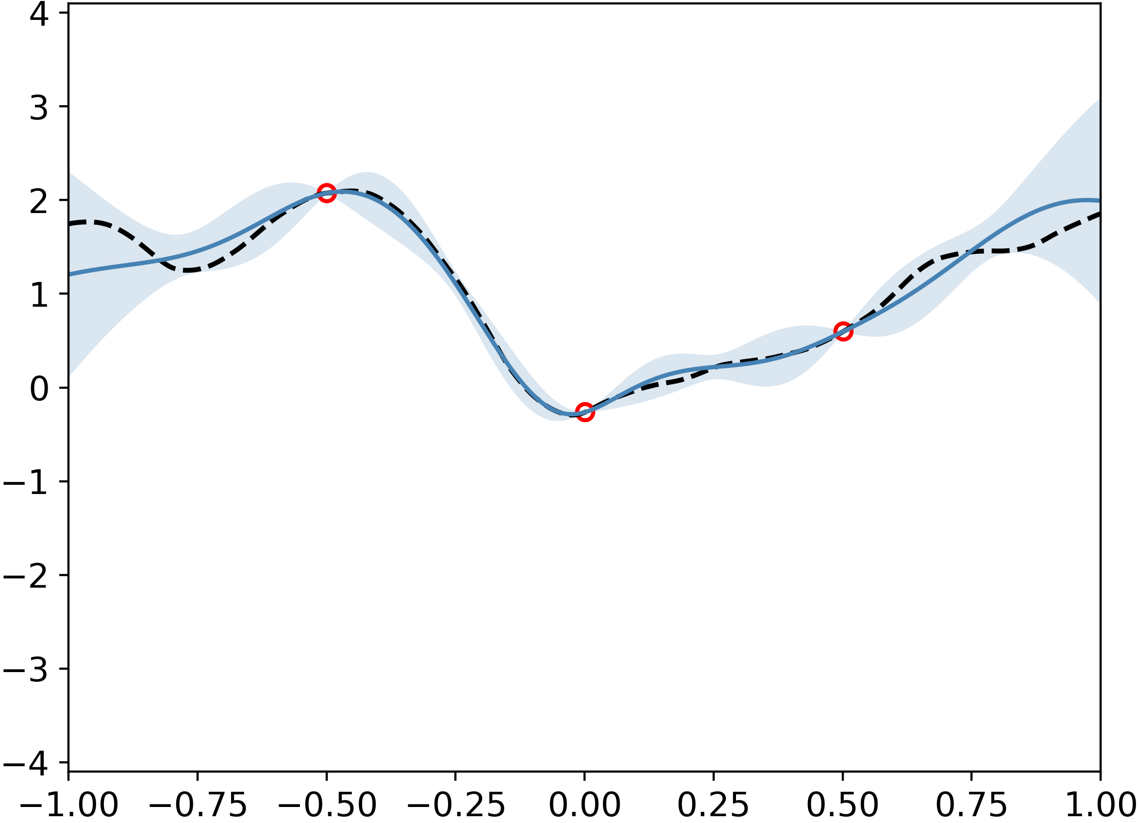
(a)

Figure 2: Continuation of the introductory example with addition of derivative observation at $x=0$.

Now, $H_{2}([-1,1])$ is a RKHS and thus by Theorem 3 the Gaussian measure - Gaussian process correspondence is applicable. Furthermore, the 7 observations (3 pointwise + 1 integral + 2 Fourier + 1 derivative) considered can be described by a bounded operator between separable Banach spaces $G:H_{2}([-1,1])\rightarrow\mathbb{R}^{7}$, so that the disintegration framework from Section 3 can be used. Finally, using the updated formulae (Corollary 7) one can express the posterior mean and covariance after inclusion of the derivative observation as an update of the one after assimilation of the previous observations:

$$\tilde{m}^{(7)}_{x_{0}}(y_{7}) =\tilde{m}_{x_{0}}^{(6)}(y_{1},...,y_{6})$$

$$\phantom{--}+\frac{d}{dx}\tilde{k}^{(6)}(x_{0},x)|_{x=0}\left(\frac{d}{dx}\frac{d}{dx^{\prime}}\tilde{k}^{(6)}(x,x^{\prime})|_{x,x^{\prime}=0}\right)^{-1}(y_{7}-\frac{d}{dx}\tilde{m}_{x}^{(6)}(y_{1},...,y_{6})|_{x=0})$$

$$\tilde{k}^{(7)}(x_{1},x_{2}) =\tilde{k}^{(6)}(x_{1},x_{2})-\frac{d}{dx}\tilde{k}^{(6)}(x_{1},x)|_{x=0}\left(\frac{d}{dx}\frac{d}{dx^{\prime}}\tilde{k}^{(6)}(x,x^{\prime})|_{x,x^{\prime}=0}\right)^{-1}\frac{d}{dx}\tilde{k}^{(6)}(x,x_{2})|_{x=0}$$

where $\tilde{m}_{x_{0}}^{(6)}(y_{1},...,y_{6})$ and $\tilde{k}^{(6)}(x_{1},x_{2})$ denote the mean and covariance function after inclusion of the first 6 observations. Note that the correspondence between the mean element and covariance operator of the induced measure and the mean and covariance function of the process (Lemma 1) can be used since the Dirac delta functionals belong to the dual of $H_{2}([-1,1])$. This example demonstrates how the Gaussian measure framework can be used to provide a thorough theoretical grounding to previously known techniques [42, 36, 1].

4 Conclusion

By bridging recent results about GP sample path properties with the framework of Gaussian measures, we provide a formulation of sequential data assimilation of linear operator data under Gaussian models in the language of disintegrations of measures. We show equivalence of the Gaussian process and Gaussian measure approaches and generalize the GP update formulae to disintegrations. While providing a purely functional formulation of the assimilation process, the framework of disintegrations also allows for a more rigorous abstract treatment of the conditional law. This can be leveraged to provide fast update formulae for GP under linear operator observations [50] and we hope it can serve as foundations for further theoretical enquiries and practical developments in probabilistic function modelling.

Appendix A Proofs of Equivalence of Gaussian Process and Gaussian measure

We here briefly recall the theorems and definitions needed to prove our main results, and present the proofs. For the functional analysis background, we refer the reader to Folland, [17] and to Tarieladze and Vakhania, [49], Vakhania et al., [51] for the background about Gaussian measures. The theorems for equivalence between Gaussian processes and Gaussian measures are adapted from Rajput and Cambanis, [34], while the one for conditioning / disintegration of Gaussian measures are adapted from Tarieladze and Vakhania, [49].

Most of this chapter will be concerned with random variables taking values in the space of continuous function $C(D)$, where $D$ is a compact metric space. When endowed with the sup-norm, $C(D)$ turns into a Banach space. This space enjoys two useful properties:

1. $C(D)$ is separable, and as a consequence, the Borel $\sigma$-algebra and the cylindrical $\sigma$-algebra on $C(D)$ agree.

2. The dual space $C(D)^{*}$ is the space of Radon measures on $D$ and (by Riesz-Markov-Kakutani [37]) for all $\ell\in C(D)^{*}:\exists\lambda$ Radon measure on $D$ such that

   $$\forall f\in C(D):\ell(f)=\int fd\lambda.$$

In order to prove Theorem 1 and Theorem 2, we first recall a classic approximation result for continuous real-valued functions on compact metric spaces that will be useful for proving measurability properties and Gaussianity of the measure induced by a GP. For reference, see [17, Theorem 2.10].

Lemma 2.

Let $D$ be a compact metric space and $f:D\rightarrow\mathbb{R}$ be continuous. Then, there exists a sequence of simple functions $f_{n}$ converging to $f$ uniformly on $D$. For each $n$, the approximating function can be written as:

$$f_{n} =\sum_{k=0}^{K(n)}f\left(t_{k}^{(n)}\right)\mathbb{1}_{A^{(n)}_{k}},$$ (A.1)

where $K(n)\in\mathbb{N}$, $t_{k}^{(n)}\in D$ and the $A_{k}^{(n)}$’s are Borel measurable sets for all $k$.

We now show that, for stochastic processes on compact metric spaces, having continuous sample paths is enough to ensure product measurability.

Theorem 10.

Let $\left(\Omega,\mathcal{F},\mathbb{P};Z(x;\omega),x\in D\right)$ be a stochastic process on a compact metric space $D$ with continuous sample paths. Then it is measurable as a mapping $\left(D\times\Omega,~{}\mathcal{B}(D)\times\mathcal{F}\right)\rightarrow\left(\mathbb{R},~{}\mathcal{B}(\mathbb{R})\right)$ (product measurable).

Proof.

This is a direct consequence of Gowrisankaran, [19, Theorem 2]. ∎

We now have all the ingredients to prove the main theorems about equivalence of process and measure.

Proof.

(Theorem 1) By Theorem 10, the only thing left to prove is that for all $\ell\in C(D)^{*}$ the real random variable $\ell\circ\Phi$ is Gaussian.
By the Riesz-Markov representation theorem, there exists a Radon measure $\lambda$ on $D$ representing $\ell$. Now, for each $\omega\in\Omega$, we use Lemma 2 to get a uniform approximation $Z_{n}(\cdot;\omega)\rightarrow Z(\cdot;\omega)$ as in Equation A.1. We then have:

$$\ell\circ\Phi(\omega) =\ell\left(\lim_{n\rightarrow\infty}Z_{n}\left(\cdot;\omega\right)\right)=\lim_{n\rightarrow\infty}\int\sum_{k=0}^{K(n)}Z\left(t^{(n)}_{k};\omega\right)\mathbb{1}_{A^{(n)}_{k}}d\lambda$$

$$=\lim_{n\rightarrow\infty}\sum_{k=0}^{K(n)}Z\left(t^{(n)}_{k};\omega\right)\lambda\left(A^{(n)}_{k}\right).$$

Now, as a convergent series of Gaussian random variables, the above is Gaussian (use characteristic functions and Lévy convergence theorem). ∎

We now turn to the proof of Theorem 2.

Proof.

(Theorem 2) Let $\Omega=C(D)$ and $\mathcal{F}$ be the Borel sigma algebra on $C(D)$ and define a collection of random variables

$$Z_{s}:\left(\Omega,\mathcal{F},\mu\right)\rightarrow\left(\mathbb{R},\mathcal{B}\left(\mathbb{R}\right)\right),~{}\omega\mapsto\delta_{s}\left(\omega\right)$$

for all $s\in D$. Since for all $s\in D$, the Dirac functionals $\delta_{s}$ belong to the dual of $C(D)$, we have that $Z_{t}$ is a Gaussian real random variable for all $s$. Now, for $s_{1},...,s_{n}\in D$, any linear combination of the components of the vector $\left(Z_{s_{1}},...,Z_{s_{n}}\right)$ may be written an element of $C(D)^{*}$, and will hence be Gaussian distributed by Gaussianity of the measure. This shows that $Z$ is a Gaussian process on $D$. ∎

From the above theorems, it is also clear that if $Z$ is the process induced by a Gaussian measure on $C(D)$, then for any $s\in D$, we have

$$\mathbb{E}_{\mu}\left[f(s)\right]=\mathbb{E}\left[Z_{s}\right]$$ (A.2)

and the same is true if $Z$ is a GP on $D$ with trajectories in $C(D)$ and $\mu$ is the measure induced by the process. This allows us to translate everything from process to measure and back without needing to worry about the details. Finally, using the fact that the Dirac deltas belong to the dual we may also prove Lemma 1 about the correspondence between mean element and covariance operator of the induced measure and mean and covariance function of the process.

Proof.

(Lemma 1) For $s,s_{1},s_{2}\in D$, let:

$$m_{s}: =\langle m_{\mu},\delta_{s}\rangle=\int_{C(D)}f(s)d\mu(f)=\mathbb{E}_{\mu}\left[f(s)\right]=\mathbb{E}\left[Z_{s}\right]$$

$$k(s_{1},s_{2}): =\langle\delta_{s_{1}},C_{\mu}\delta_{s_{2}}\rangle=\delta_{s_{1}}\left[\int_{C(D)}f(s_{2})fd\mu(f)-m_{s_{1}}m_{\mu}\right]$$

$$=\mathbb{E}_{\mu}\left[f(s_{1})f(s_{2})\right]-\mathbb{E}_{\mu}\left[f(s_{1})\right]\mathbb{E}\left[f(s_{2})\right]$$

$$=\mathbb{E}\left[Z_{s_{1}}Z_{s_{2}}\right]-\mathbb{E}\left[Z_{s_{1}}\right]\mathbb{E}\left[Z_{s_{2}}\right].$$

Note that exchanging Dirac deltas and integration is allowed by Fubini since Gaussian measures are finite and the last equalities are consequences of Equation A.2. ∎

The extension of Theorem 1 and Theorem 2 to processes and measures on RKHS is straightforward. Indeed, the measure-to-process correspondence follows directly from the fact that the evaluation functionals belong to the dual of the RKHS. For the process-to-measure correspondence, the crucial property is the Gaussianity of linear functionals of the field, which in a RKHS $\mathcal{H}$ is automatically satisfied since any linear functional can be expressed as an infinite linear combination of reproducing kernel values, which in turn act as evaluation functionals:

$$\left\langle\ell,Z\right\rangle =\left\langle\sum_{i=1}^{\infty}a_{i}k(x_{i},\cdot),Z\right\rangle_{\mathcal{H}}=\sum_{i=1}^{\infty}a_{i}Z_{x_{i}},$$

which, as a convergent sum of Gaussian random variables, is Gaussian.

Appendix B Conditioning, Disintegration and Link to Finite-Dimensional Formulation:

We now turn to the proof of Theorem 6.

Proof.

(Theorem 6) To prove the theorem, we have to adapt the proof of Tarieladze and Vakhania, [49][Theorem 3.11] to the non-centered case. Compared to the original theorem, the conditional covariance operator $\tilde{C}_{\mu}$ hasn’t changed, whereas the conditional mean $\tilde{m}_{\mu}\left(y\right)$ clearly still defines a continuous mapping satisfying $G\tilde{m}_{\mu}\left(y\right)=y$ for all $y$ in the range of $C_{\nu}$. Hence, for all $y\in Y$, we can still use Tarieladze and Vakhania, [49][Lemma 3.8] to define $\mu_{|G=y}$ as a Gaussian measure having mean element $\tilde{m}_{\mu}\left(y\right)$ and covariance operator $\tilde{C}_{\mu}$. What is left to check is that it satisfies the conditions in Definition 2 to be a disintegration of $\mu$ with respect to $G$.

In the following, let $y\in Y$ and $A\in\mathcal{A}$ be arbitrary.

• The measurability of the mapping $y\mapsto\mu_{|G=y}\left(A\right)$ for fixed $A$ holds since, compared to the centered case, the conditional mean $\tilde{m}_{\mu}\left(y\right)$ is only translated by an element that does not depend on $y$.

• Define $Y_{0}:=Gm_{\mu}+C_{\nu}\left(Y^{*}\right)$. We have $\mu\circ G^{-1}\left(Y_{0}\right)=1$ by Tarieladze and Vakhania, [49][Lemma 3.3] and Tarieladze and Vakhania, [49][Corollary 3.7]. Following the exact same reasoning as in the proof of Tarieladze and Vakhania, [49][Theorem 3.11] we have that $\mu_{y}\left(G^{-1}\left(y\right)\right)=1$.

• By Tarieladze and Vakhania, [49][Proposition 3.2], the last thing we have to check is that

  $$\hat{\mu}\left(x^{*}\right)=\int_{Y}\hat{\mu}_{|G=y}\left(x^{*}\right)d\nu\left(y\right),~{}\forall x^{*}\in X^{*},$$

  where $\hat{\mu}\left(\bm{\cdot}\right)$ denotes the characteristic functional of $\mu$ (see Tarieladze and Vakhania, [49][Section 3.2]. Compared to the original proof, only the mean element is changed, so for the sake of simplicity we only consider the steps of the proof that differ from the original ones.
  We have that

  $$\int_{Y}\exp\left[i\left\langle\tilde{m}_{\mu}\left(y\right),x^{*}\right\rangle\right]d\nu\left(y\right) =\exp\left[i\left\langle m_{\mu},x^{*}\right\rangle\right]$$

  $$\cdot\int_{y}\exp\left[i\left\langle\sum_{i=1}^{n}\left\langle y-Gm_{\mu},y_{i}^{*}\right\rangle C_{\mu}G*y_{i}^{*},x^{*}\right\rangle\right]d\nu\left(y\right),$$

  which, after a change of variable $y\mapsto y-Gm_{\mu}$ can be seen to be the characteristic function of a centered Gaussian measure with covariance $C_{\mu}$ by following the same argument as in the original proof (the same argument is presented in more detail in the proof of the next theorem).

∎

The last theorem we have to prove is the one about the transitivity of disintegrations.

Proof.

(Theorem 7) By unicity of disintegrations [49][Remark 3.12], we only have to prove that the family

$$\left(\left(\mu_{|G_{1}=y_{1}}\right)_{|G_{2}=y_{2}}\right)_{\left(y_{1},y_{2}\right)\in Y_{1}\bigoplus Y_{2}}$$

defines a disintegration of $\mu$ with respect to $\left(G_{1},G_{2}\right)$.
First a word of caution: there exist no canonical norm on the direct sum of Banach spaces. However, there are several norms on the direct sum that induce the product topology [9][Exercice 1.30]. We here work with any of these. Then, the Borel $\sigma$-algebra on the direct sum is given by the product of the Borel $\sigma$-algebras of the components [7][p.244].

Here, by construction, for any $\left(y_{1},y_{2}\right)\in Y_{1}\bigoplus Y_{2}$, the measure $\left(\mu_{|G_{1}=y_{1}}\right)_{|G_{2}=y_{2}}$ is defined as a Gaussian measure having mean element

$$\tilde{m}_{\mu}^{(1)}\left(y_{1}\right)+\sum_{i=1}^{p_{2}}\left\langle y_{2}-G_{2}\tilde{m}_{\mu}^{(1)}\left(y_{1}\right),y_{i}^{(2)*}\right\rangle\tilde{C}_{\mu}^{(1)}G_{2}^{*}y_{i}^{(2)*},$$

and covariance operator

$$\tilde{C}_{\mu}^{(1,2)}: =\tilde{C}_{\mu}^{(1)}-\sum_{i=1}^{p_{2}}\left\langle\tilde{C}_{\mu}^{(1)}G_{2}^{*}y_{i}^{(2)*},\cdot\right\rangle\tilde{C}_{\mu}^{(1)}G_{2}^{*}y_{i}^{(2)*},$$

where $\tilde{m}_{\mu}^{(1)}$ and $\tilde{C}_{\mu}^{(1)}$ denote the mean element and covariance operator of $\mu_{|G_{1}=y_{1}}$ and $(y_{i}^{(2)*})_{i=1,...,p_{2}}$ is any representing sequence for the operator $G_{2}\tilde{C}_{\mu}^{(1)}G_{2}^{*}$. Note that the assumption that $C_{\nu_{2}}$ has finite rank implies that the aforementioned operator also has finite rank. Since for all $y_{1}\in Y_{1}$ the measure $\mu_{|G_{1}=y_{1}}$ is Gaussian, we have by Theorem 6 that $\left(\mu_{|G_{1}=y_{1}}\right)_{|G_{2}=y_{2}}$ is Gaussian.

As in the previous proof, we have to check the three conditions of Definition 2.

• For fixed $A$, the mapping $\left(y_{1},y_{2}\right)\mapsto\left(\mu_{|G_{1}=y_{1}}\right)_{G_{2}=y_{2}}\left(A\right)$ is an addition of a $\mathcal{B}\left(Y_{1}\right)$-measurable mapping with a $\mathcal{B}\left(Y_{2}\right)$-measurable mapping, and, as such, measurable with respect to the product $\sigma$-algebra.

• Let $Y:=Y_{1}\bigoplus Y_{2}$ and note that $Y^{*}=Y_{1}^{*}\bigoplus Y_{2}^{*}$ (dual of direct sum is the direct sum of the duals). Then define $Y_{0}=Gm_{\mu}+GC_{\mu}G^{*}\left(Y_{1}^{*}\bigoplus Y_{2}^{*}\right)$. Note that the Gaussian measure $\mu\circ G^{-1}$ has mean $Gm_{\mu}$ and covariance operator $GC_{\mu}G^{*}$, hence $\mu\circ G^{-1}\left(Y_{0}\right)=1$ by Tarieladze and Vakhania, [49][Lemma 3.3].

  For any $\left(y_{1},y_{2}\right)\in Y_{0}$ we have that the Gaussian measure $\left(\mu_{|G_{1}=y_{1}}\right)_{|G_{2}=y_{2}}\circ G^{-1}$ has covariance operator $G\tilde{C}_{\mu}^{(1,2)}G^{*}$. Computing the operator componentwise, we have that:

  $$\textasciiacute G_{2}\tilde{C}_{\mu}^{(1,2)}G_{2}^{*} =G_{2}\tilde{C}_{\mu}^{(1)}G_{2}^{*}-\sum_{i=1}^{p_{2}}\left\langle\tilde{C}_{\mu}^{(1)}G_{2}^{*}y_{i}^{(2)*},G_{2}^{*}\right\rangle G_{2}\tilde{C}_{\mu}^{(1)}G_{2}^{*}y_{i}^{(2)*}=0,$$

  where the last equality follows from Tarieladze and Vakhania, [49][Lemma 3.4, (c)] since $y_{i}^{(2)*}$ is a $G_{2}\tilde{C}_{\mu}^{(1)}G_{2}^{*}$-representing sequence. An analogous computation for the other components shows that they all vanish.

Defining $\mu^{(1,2)}_{y_{1},y_{2}}:=\left(\mu_{|G_{1}=y_{1}}\right)_{|G_{2}=y_{2}}$, the last point to show is that

$$\hat{\mu}\left(x^{*}\right) =\int_{Y_{1}}\int_{Y_{2}}\hat{\mu}^{(1,2)}_{y_{1},y_{2}}\left(x^{*}\right)d\nu_{1}\left(y_{1}\right)d\nu_{2}\left(y_{2}\right),~{}\forall x^{*}\in C(D)^{*},$$

where we have defined the measures $\nu_{1}:=\mu\circ G_{1}^{-1}$ and $\nu_{2}:=\mu_{|G_{1}=y_{1}}\circ G_{2}^{-1}$, omitting the dependence on $y_{1}$ for simplicity. Using the fact that $\mu_{|G_{1}=y_{1}}$ is a disintegration of $\mu$ with respect to $G_{1}$, defining $x_{j}^{(2)*}:=G_{2}^{*}y^{(2)*}$ and performing a change of variables, we have that

$$\int_{Y_{1}}\int_{Y_{2}}\hat{\mu}^{(1,2)}_{y_{1},y_{2}}\left(x^{*}\right)d\nu_{1}\left(y_{1}\right)d\nu_{2}\left(y_{2}\right) =\hat{\mu}\left(x^{*}\right)+\int_{Y_{1}}\int_{Y_{2}}\exp\left[i\sum_{j}\left\langle y_{2},y_{j}^{(2)*}\right\rangle\left\langle C_{\mu}x_{j}^{(2)*},x^{*}\right\rangle\right.$$

$$+\left.\frac{1}{2}\sum_{j}\left\langle C_{\mu}^{(1)}x_{j}^{(2)*},x^{*}\right\rangle\left\langle C_{\mu}^{(1)}x_{j}^{(2)*},x^{*}\right\rangle\right].$$

Now defining $M\left(y_{2}\right):=\sum_{j}\left\langle y_{2},y_{j}^{(2)*}\right\rangle C_{\mu}^{(1)}x_{j}^{(2)}$ and $R_{1}:=\sum_{j}\left\langle C_{\mu}^{(1)}x_{j}^{(2)*},\cdot\right\rangle C_{\mu}^{(1)}x_{j}^{(2)*}$ (which can be thought of as conditional means and covariance operator), the remaining integral reduces to:

$$\int_{Y_{1}}\int_{Y_{2}}\exp\left[i\left\langle M\left(y_{2}\right),x^{*}\right\rangle+\frac{1}{2}R_{1}x^{*}\right]d\nu_{1}\left(y_{1}\right)d\nu_{2}\left(y_{2}\right).$$

We can simplify the first summand by noticing that it amounts to the characteristic function of a Gaussian measure:

$$\int_{Y_{2}}\exp\left[i\left\langle M\left(y_{2}\right),x^{*}\right\rangle\right]d\nu_{2}\left(y_{2}\right) =\hat{\nu}_{2}\left(M^{*}\left(x^{*}\right)\right)=\int_{Y_{2}}\exp\left[-\frac{1}{2}\left\langle C_{\nu_{2}}M^{*}\left(x^{*}\right),M^{*}\left(x^{*}\right)\right\rangle\right]$$

$$=\int_{Y_{2}}\exp\left[-\frac{1}{2}\sum_{j}\left\langle C_{\mu}^{(1)}x_{j}^{(2)*},x^{*}\right\rangle^{2}\right]d\nu_{2}\left(y_{2}\right)$$

$$=\int_{Y_{2}}\exp\left[-\frac{1}{2}R_{1}x^{*}\right]d\nu_{2}\left(y_{2}\right),$$

where the penultimate equality follows from $C_{\nu_{2}}$-orthogonality of the $y_{i}^{(2)*}$ sequence. This concludes the proof. Note when computing the characteristic function of $\nu_{2}$, we have omitted the mean term due to the change of variable performed earlier (to be perfectly rigorous, one should use a different notation for the transformed measure). ∎

Link to Finite Dimensional case When the inversion data is finite-dimensional, that is the observation operator $G$ maps into $\mathbb{R}^{n}$ and $\mathbb{R}^{n}$ is considered as a Banach space with respect to the $2$-norm. One can then canonically identify $\mathbb{R}^{n}$ with its dual using the dot product: $v\mapsto\langle v,\cdot\rangle$. In the following, when elements of $\mathbb{R}^{n}$ are involved, the duality bracket $\langle\cdot,\cdot\rangle$ will denote the dot product, also, $e_{i},i=1,...,n$ will be used to denote the canonical basis of $\mathbb{R}^{n}$. We now prove that $y_{i}:=C_{\nu}^{-1/2}e_{i},~{}i=1,...,n$ forms a $C_{\nu}$-representing sequence.

Proof.

(Remark 4) First of all, the $y_{i}$ form a $C_{\nu}$-orthonormal family since

$$\langle C_{\nu}y_{i},y_{j}\rangle =\langle C_{\nu}^{1/2}y_{i},C_{\nu}^{1/2}y_{j}\rangle=\langle e_{i},e_{j}\rangle=\delta_{ij},$$

where the first equality follows by self-adjointness of $C_{\nu}$. Also remember that since here we are working over $\mathbb{R}^{n}$, the duality bracket denotes the dot product and $\mathbb{R}^{n}$ is identified with its dual. Finally, according to Tarieladze and Vakhania, [49][Lemma 3.4], the last thing we have to show is that for any $v\in\mathbb{R}^{n}$: $C_{\nu}v=\sum_{i=1}^{n}\langle C_{\nu}y_{i},v\rangle C_{\nu}y_{i}$. Note that since $C_{\nu}$ is a positive self-adjoint operator, the $y_{i}$’s form a basis of $\mathbb{R}^{n}$, and we can thus write $v=\sum_{i=1}^{n}v_{i}y_{i}$ for some component $v_{i}$. Then

$$\sum_{i=1}^{n}\langle C_{\nu}y_{i},v\rangle C_{\nu}y_{i} =\sum_{i,j=1}^{n}\langle C_{\nu}y_{i},v_{j}y_{j}\rangle C_{\nu}y_{i}=v^{i}C_{\nu}y_{i}=C_{\nu}v$$

∎

Proof.

(Corollary 5) As before, let $y_{i}:=C_{\nu}^{-1/2}e_{i},~{}i=1,...,n$. In order to get closed-form formulae for the posterior under such operators, we need to be able to compute the action of the adjoint $G^{*}$. We begin by recalling the definition of the adjoint of a linear operator $T:X\rightarrow Y$ between Banach spaces:

$$T^{*}: Y^{*}\rightarrow X^{*}$$

$$y^{*}\mapsto\left(x\mapsto\langle y^{*},Tx\rangle\right).$$

Now if we consider a (bounded) linear form $G_{j}:X:\rightarrow\mathbb{R}$, then its adjoint is given by:

$$G_{j}^{*}: \mathbb{R}\rightarrow X^{*}$$

$$a\mapsto\left(f\mapsto a\cdot G_{j}f\right).$$

So the adjoint of the observation operator may be written as:

$$G^{*}:\mathbb{R}^{n} \rightarrow X^{*}$$

$$\left(a_{1},...,a_{n}\right) \mapsto\left(f\mapsto a_{1}\cdot G_{1}f+...+a_{n}\cdot G_{n}f\right).$$

There is one last computation that we need to perform before getting the mean and covariance:

$$\left\langle C_{\mu}G^{*}y^{(i)},\delta_{s}\right\rangle =\left\langle C_{\mu}\delta_{s},G^{*}y^{(i)}\right\rangle=y^{(i)}\cdot G\left(C_{\mu}\delta_{s}\right)=y^{(i)}\cdot Gk(\cdot,s)=y^{(i)}\cdot K_{sG}.$$

Putting everything together we are now able to express the covariance operator:

$$\tilde{k}(s_{1},s_{2}) =k(s_{1},s_{2})-\sum_{i=1}^{n}y^{(i)}\cdot K_{s_{1}G}y^{(i)}\cdot K_{s_{2}G}$$

$$=k(s_{1},s_{2})-\sum_{i=1}^{n}K_{s_{1}G}^{T}y^{(i)}\left(y^{(i)}\right)^{T}K_{s_{2}G}$$

$$=k(s_{1},s_{2})-\sum_{i=1}^{n}K_{s_{1}G}^{T}C_{\nu}^{-1/2}e_{i}e_{i}^{T}C_{\nu}^{-1/2}K_{s_{2}G}$$

$$=k(s_{1},s_{2})-K_{s_{1}G}^{T}K_{GG}^{-1}K_{s_{2}G}.$$

Where we have used the fact that $\sum_{i=1}^{n}e_{i}e_{i}^{T}=\bm{I}_{n}$ and that:

$$e_{i}\cdot GC_{\mu}G^{*}e_{j} =G_{i}(G_{j}k(\cdot,\cdot)).$$

Note that this last step requires one to explicitly compute the action of the $G_{i}$’s on the covariance operator $C_{\mu}$. This can be done in the case where $X=C(D)$ since the individual components on the observation operator can be written as integrals with respect to Radon measures $G_{i}f=\int_{D}f(s)d\lambda_{i}\left(s\right)$ or in the case where $X$ is a RKHS, since then the components can be written as infinite linear combinations of Dirace deltas $G_{i}f=\sum_{k=1}^{\infty}a_{k}^{(i)}f(s^{(i)}_{k})$. Computing the action on the covariance operator in the general case is not trivial. The mean can be obtained through a similar argument. ∎

Proofs for Infinite Rank Data

Proof.

(Theorem 8) As before, compared to the centered case, only the conditional mean changes. Thanks to [49, Lemma 3.5] we can still select a countably infinite $C_{\nu}$ representing sequence $\left(y_{i}\right)_{i\in\mathbb{N}}$. Now define, for all $n\in\mathbb{N}$:

$$\tilde{m}^{(n)}_{\mu}(y) =m_{\mu}+\sum_{i=1}^{n}\left\langle y-Gm_{\mu},y_{i}^{*}\right\rangle C_{\mu}G^{*}y_{i}^{*}.$$ (B.1)

Furthermore, define the spaces: $Y_{2}:=\{y\in Y:~{}\tilde{m}^{(n)}_{\mu}(y)\text{ converges}\}$, and $Y_{3}:=\{y\in Y:~{}\lim_{n\rightarrow\infty}||y-\sum_{i=1}^{n}\left\langle y-Gm_{\mu},y_{i}^{*}\right\rangle C_{\nu}y_{i}^{*}||=0\}$. We begin by showing that these subspaces of $Y$ have full measure.

Claim: $\nu(Y_{2})=1$.

Proof.

Our goal is to show that the random element $\tilde{m}_{\mu}^{n}$ converges $\nu$-almost surely in $X$. First, define $\xi_{i}:=\left\langle y-Gm_{\mu},y_{i}^{*}\right\rangle C_{\mu}G^{*}y_{i}^{*}$. Thanks to $C_{\nu}$-orthonormality, the $y_{i}^{*}$ are independent Gaussian random variables, and hence the $\xi_{i}$ too. Hence, by Ito-Nisio [51, Theorem 5.2.4], we get $\nu$-almost-sure convergence provided we can show that there exists a random probability measure $\mu^{\prime}$ on $X$ such that the joint characteristic function converges to the characteristic function of $\mu^{\prime}$:

$$\prod_{i=1}^{n}\hat{\mathbb{P}}_{\xi_{i}}\left(f\right)\rightarrow\hat{\mu^{\prime}}(f),~{}\text{all }f\in X^{*}.$$

By independence of the $\xi_{i}$, we have, for $f\in X^{*}$:

$$\prod_{i=1}^{n}\hat{\mathbb{P}}_{\xi_{i}}(f) =\int_{Y}\exp\left[i\left\langle f,\sum_{i=1}^{n}\left\langle y-Gm_{\mu},y_{i}^{*}\right\rangle C_{\mu}G^{*}y_{i}^{*}\right\rangle\right]d\nu(y)$$

$$=\int_{Y}\exp\left[i\left\langle y^{\prime},\sum_{i=1}^{n}y_{i}^{*}\left\langle f,C_{\mu}G^{*}y_{i}^{*}\right\rangle\right\rangle\right]d\nu^{\prime}(y^{\prime}),$$

where we have performed a change of variable $y^{\prime}:=y-Gm_{\mu}$ and hence $\nu$’ is a centred Gaussian measure with covariance operator $C_{\nu}$. Now, using the characteristic function of Gaussian measures, the above is equal to:

$$\hat{\nu}\left(\sum_{i=1}^{n}y_{i}^{*}\left\langle f,C_{\mu}G^{*}y_{i}^{*}\right\rangle\right) =\exp\left[-\frac{1}{2}\sum_{i,j=1}^{n}\left\langle f,C_{\mu}G^{*}y_{i}^{*}\right\rangle\left\langle f,C_{\mu}G^{*}y_{j}^{*}\right\rangle\left\langle C_{\nu}y_{i}^{*},y_{j}^{*}\right\rangle\right]$$

$$=\exp\left[-\frac{1}{2}\sum_{i=1}^{n}\left\langle f,C_{\mu}G^{*}y_{i}^{*}\right\rangle^{2}\right],$$

where the last equality follows from $C_{\nu}$-orthonormality of the representing sequence. We thus have:

$$\lim_{n\rightarrow\infty}\prod_{i=1}^{n}\hat{\mathbb{P}}_{\xi_{i}}(f) =\exp\left[-\frac{1}{2}\left\langle R_{1}f,f\right\rangle\right],$$ (B.2)

where $R_{1}:=\lim_{n\rightarrow\infty}\sum_{i=1}^{\infty}\left\langle C_{\mu}G^{*}y_{i}^{*},\bullet\right\rangle C_{\mu}G^{*}y_{i}^{*}$ is a Gaussian covariance by [49, Lemma 3.4 and Proposition 3.9]. The Claim follows from the fact that for any Gaussian covariance, there exists a Gaussian measure having that covariance as covariance operator [49, Lemma 3.8]. ∎

Claim: $\nu(Y_{3})=1$.

Proof.

Note that if $y-Gm_{\mu}$ can be written as $C_{\nu}y^{*}$ for some $y^{*}\in Y^{*}$, then it immediatly follows, by [49, Lemma 3.4], that:

$$\sum_{i=1}^{\infty}\left\langle y-Gm_{\mu},y_{i}^{*}\right\rangle C_{\nu}y_{i}^{*} =\sum_{i=1}^{\infty}\left\langle y^{*},C_{\nu}y_{i}^{*}\right\rangle C_{\nu}y_{i}^{*}=C_{\nu}y^{*}=y-Gm_{\mu}.$$

Now, the subspace whose elements can be written as above is exatly the Cameron-Martin space $C_{\nu}\left(Y^{*}\right)$. While this is a $\nu$-null space, it is a well-known fact that its closure in $Y$ has full measure, so that there exists a subset of full measure whose elements can be approximated by elements of $C_{\nu}\left(Y^{*}\right)$ and thus the defining property of $Y_{3}$ holds on a set of full measure. ∎

Now, we define $Y_{0}:=Y_{2}\cap Y_{3}$. We construct a disintegration $\left(\mu_{|G=y}\right)_{y\in Y_{0}}$ as in the finite rank case, but now restricting to the subspace $Y_{0}$ where the conditional mean is defined. What is left to check is that it satisfies the three defining properties of disintegrations (Definition 2). Property 1 holds as in the finite rank case. For Property 2, we notice that, for any $y\in Y_{0}$:

$$G\tilde{m}_{\mu}(y) =\lim_{n\rightarrow\infty}\tilde{m}_{\mu}^{(n)}(y)=Gm_{\mu}-\sum_{i=1}^{\infty}\left\langle Gm_{\mu},y_{i}^{*}\right\rangle C_{\nu}y_{i}^{*}+\sum_{i=1}^{\infty}\left\langle y,y_{i}^{*}\right\rangle C_{\nu}y_{i}^{*}=y,$$

since $Gm_{\mu}$ is the mean of $\nu$ and thus belongs to the Cameron-Martin space. Finally, for Property 3, thanks to [49, Proposition 3.2], we only have to show that the characteristic function of $\mu$ writes as a mixing of the characteristic functions of the conditionals, i.e. that:

$$\hat{\mu}(f) =\int_{Y}\hat{\mu}_{|G=y}(f)d\nu(y),\text{ all }f\in X^{*}.$$

Now, for $y\in Y_{0}$, we have that $\mu_{|G=y}$ is Gaussian, with mean $\tilde{m}_{\mu}(y)$ and covariance operator $C_{\mu}-R_{1}$. Hence, we have:

$$\int_{Y}\hat{\mu}_{|G=y}(f)d\nu(y) =\int_{Y}\exp\left[i\left\langle\tilde{m}_{\mu}(y),f\right\rangle-\frac{1}{2}\left\langle C_{\mu},f\right\rangle+\frac{1}{2}\left\langle R_{1}f,f\right\rangle\right]d\nu(y)$$

$$=\exp\left[i\left\langle m_{\mu},f\right\rangle-\frac{1}{2}\left\langle C_{\mu}f,f\right\rangle\right]=\hat{\mu}(f),$$

where the second-to-last equality follow from Equation B.2. This completes the proof in the infinite rank case. ∎

Appendix C Explicit Update Formulae for Mean Element and Covariance Operator

For the sake of completeness, we here provide detailed update formulae for the mean element and covariance operator, as a direct consequence of Theorem 7.

Corollary 8.

Consider the setting of Theorem 7 and let $(y_{i}^{*(12)})_{i=1,...,p_{12}}$ be a $GC_{\mu}G^{*}$-representing sequence, $(y_{i}^{*(1)})_{i=1,...,p_{1}}$ be a $G_{1}C_{\mu}G_{1}^{*}$-representing sequence and $(y_{i}^{*(2)})_{i=1,...,p_{2}}$ be a $G_{2}C^{(1)}_{\mu}G_{2}^{*}$-representing sequence. Then we have:

$$C_{\mu}-\sum_{i=1}^{p_{12}}\left\langle C_{\mu}G^{*}y_{i}^{(12)},\bullet\right\rangle C_{\mu}G^{*}y_{i}^{*(12)} =C_{\mu}-\sum_{i=1}^{p_{1}}\left\langle C_{\mu}G^{*}y_{i}^{*(1)},\bullet\right\rangle C_{\mu}G_{1}^{*}y_{i}^{*(1)}-\sum_{j=1}^{p_{2}}\left\langle C_{\mu}G_{2}^{*}y_{j}^{*(2)},\bullet\right\rangle C_{\mu}G_{2}^{*}y_{j}^{*(2)}$$

$$+\sum_{j=1}^{p_{2}}\sum_{i=1}^{p_{1}} \left\langle C_{\mu}G_{2}^{*}y_{j}^{*(2)},\bullet\right\rangle\left\langle C_{\mu}G_{1}^{*}y_{i}^{*(1)},G_{2}^{*}y_{j}^{*(2)}\right\rangle C_{\mu}G^{*}y_{i}^{*(1)}$$

$$-\sum_{j=1}^{p_{2}}\sum_{i=1}^{p_{1}}\sum_{k=1}^{p_{1}} \left\langle C_{\mu}G_{1}^{*}y_{i}^{*(1)},G_{2}^{*}y_{j}^{*(2)}\right\rangle\left\langle C_{\mu}G_{1}^{*}y_{i}^{*(1)},\bullet\right\rangle\left\langle C_{\mu}G_{1}^{*}y_{i}^{*(1)},G_{2}^{*}y_{j}^{*(2)}\right\rangle C_{\mu}G_{1}^{*}y_{i}^{*(1)},$$

and the equality is independent of the choice of the representing sequences.

As for the mean element, we have:

$$m_{\mu}+\sum_{i=1}^{p}\left\langle y-Gm_{\mu},y_{i}^{*(12)}\right\rangle C_{\mu}G^{*}y_{i}^{*(12)}=m_{\mu}+\sum_{i=1}^{p_{1}}\left\langle y_{1}-G_{1}m_{\mu},y_{i}^{*(1)}\right\rangle C_{\mu}G_{1}^{*}y_{i}^{*(1)}$$

$$+\sum_{j=1}^{p_{2}}\left\langle y_{2},y_{j}^{*(2)}\right\rangle C_{\mu}G_{2}^{*}y_{j}^{*(2)}-\sum_{j=1}^{p_{2}}\sum_{i=1}^{p_{1}}\left\langle y_{2},y_{j}^{*(2)}\right\rangle\left\langle C_{\mu}G_{1}^{*}y_{i}^{*(1)},G_{2}^{*}y_{j}^{*(2)}\right\rangle C_{\mu}G_{1}^{*}y_{i}^{*(1)}$$

$$-\sum_{j=1}^{p_{2}}\left\langle G_{2}m_{\mu},y_{j}^{*(2)}\right\rangle C_{\mu}G_{2}^{*}y_{j}^{*(2)}$$

$$-\sum_{j=1}^{p_{2}}\sum_{i=1}^{p_{1}}\left\langle G_{2}C_{\mu}G_{1}^{*}y_{i}^{*(1)},y_{j}^{*(2)}\right\rangle\left\langle y_{1}-G_{1}m_{\mu},y_{i}^{*(1)}\right\rangle C_{\mu}G_{2}^{*}y_{j}^{*(2)}$$

$$+\sum_{j=1}^{p_{2}}\sum_{k=1}^{p_{1}}\left\langle G_{2}m_{\mu},y_{j}^{*(2)}\right\rangle\left\langle C_{\mu}G_{1}^{*}y_{k}^{*(1)},G_{2}^{*}y_{j}^{*(2)}\right\rangle C_{\mu}G_{1}^{*}y_{k}^{*(1)}$$

$$+\sum_{i=1}^{p_{2}}\sum_{i=j}^{p_{1}}\sum_{k=1}^{p_{1}}\left\langle G_{2}C_{\mu}G_{1}^{*}y_{i}^{*(1)},y_{j}^{*(2)}\right\rangle\left\langle y_{1}-G_{1}m_{\mu},y_{i}^{*(1)}\right\rangle\left\langle C_{\mu}G_{1}^{*}y_{k}^{*(1)},G_{2}^{*}y_{j}^{*(2)}\right\rangle C_{\mu}G_{1}^{*}y_{k}^{*(1)}.$$

References

• Agrell, [2019] Agrell, C. (2019). Gaussian processes with linear operator inequality constraints. Journal of Machine Learning Research, 20(135):1–36.
• Aronszajn, [1950] Aronszajn, N. (1950). Theory of reproducing kernels. Transactions of the American Mathematical Society, 68(3):337–404.
• Attia et al., [2018] Attia, A., Alexanderian, A., and Saibaba, A. (2018). Goal-oriented optimal design of experiments for large-scale Bayesian linear inverse problems. Inverse Problems, 34.
• Barnes and Watson, [1992] Barnes, R. J. and Watson, A. (1992). Efficient updating of kriging estimates and variances. Mathematical Geology, 24(1):129–133.
• Bect et al., [2019] Bect, J., Bachoc, F., and Ginsbourger, D. (2019). A supermartingale approach to Gaussian process based sequential design of experiments. Bernoulli, 25(4A):2883 – 2919.
• Berlinet and Thomas-Agnan, [2004] Berlinet, A. and Thomas-Agnan, C. (2004). Reproducing kernel Hilbert spaces in probability and statistics. Kluwer Academic Publishers.
• Billingsley, [1999] Billingsley, P. (1999). Convergence of probability measures. Wiley, New York.
• Bogachev, [1998] Bogachev, V. I. (1998). Gaussian measures. Number 62. American Mathematical Soc.
• Bühler and Salamon, [2018] Bühler, T. and Salamon, D. A. (2018). Functional analysis. American Mathematical Society, Providence, Rhode Island.
• Cambanis, [1973] Cambanis, S. (1973). On some continuity and differentiability properties of paths of gaussian processes. Journal of Multivariate Analysis, 3(4):420–434.
• Chevalier et al., [2014] Chevalier, C., Ginsbourger, D., and Emery, X. (2014). Corrected kriging update formulae for batch-sequential data assimilation. In Pardo-Igúzquiza, E., Guardiola-Albert, C., Heredia, J., Moreno-Merino, L., Durán, J., and Vargas-Guzmán, J., editors, Mathematics of Planet Earth. Lecture Notes in Earth System Sciences. Springer, Berlin, Heidelberg.
• Cotter et al., [2013] Cotter, S. L., Roberts, G. O., Stuart, A. M., and White, D. (2013). Mcmc methods for functions: modifying old algorithms to make them faster. Statistical Science, pages 424–446.
• Dashti and Stuart, [2016] Dashti, M. and Stuart, A. M. (2016). The Bayesian approach to inverse problems. Handbook of Uncertainty Quantification, pages 1–118.
• Driscoll, [1973] Driscoll, M. F. (1973). The reproducing kernel hilbert space structure of the sample paths of a gaussian process. Zeitschrift für Wahrscheinlichkeitstheorie und Verwandte Gebiete, 26:309–316.
• Emery, [2009] Emery, X. (2009). The kriging update equations and their application to the selection of neighboring data. Computational Geosciences, 13(3):269–280.
• Ernst et al., [2014] Ernst, O. G., Sprungk, B., and Starkloff, H.-J. (2014). Bayesian Inverse Problems and Kalman Filters, pages 133–159. Springer International Publishing, Cham.
• Folland, [2013] Folland, G. B. (2013). Real analysis: modern techniques and their applications. John Wiley & Sons.
• Gao et al., [1996] Gao, H., Wang, J., and Zhao, P. (1996). The updated kriging variance and optimal sample design. Mathematical Geology, 28(3):295–313.
• Gowrisankaran, [1972] Gowrisankaran, K. (1972). Measurability of functions in product spaces. Proceedings of the American Mathematical Society, 31(2):485–488.
• Hendriks et al., [2018] Hendriks, J. N., Jidling, C., Wills, A., and Schön, T. B. (2018). Evaluating the squared-exponential covariance function in gaussian processes with integral observations.
• Huber, [2014] Huber, M. F. (2014). Recursive gaussian process: On-line regression and learning. Pattern Recognition Letters, 45:85–91.
• Jackson, [1979] Jackson, D. D. (1979). The use of a priori data to resolve non-uniqueness in linear inversion. Geophysical Journal International, 57(1):137–157.
• Jidling et al., [2019] Jidling, C., Hendriks, J., Schön, T. B., and Wills, A. (2019). Deep kernel learning for integral measurements.
• Jidling et al., [2018] Jidling, C., Hendriks, J., Wahlström, N., Gregg, A., Schön, T. B., Wensrich, C., and Wills, A. (2018). Probabilistic modelling and reconstruction of strain. Nuclear Instruments and Methods in Physics Research Section B: Beam Interactions with Materials and Atoms, 436:141–155.
• Jidling et al., [2017] Jidling, C., Wahlström, N., Wills, A., and Schön, T. B. (2017). Linearly constrained Gaussian processes. In Advances in Neural Information Processing Systems, pages 1215–1224.
• Jones et al., [1998] Jones, D. R., Schonlau, M., and Welch, W. J. (1998). Efficient Global Optimization of Expensive Black-Box Functions. Journal of Global Optimization, 13(4):455–492.
• Kanagawa et al., [2018] Kanagawa, M., Hennig, P., Sejdinovic, D., and Sriperumbudur, B. K. (2018). Gaussian processes and kernel methods: A review on connections and equivalences. ArXiv, abs/1807.02582.
• Karvonen, [2021] Karvonen, T. (2021). Small sample spaces for gaussian processes. arXiv preprint arXiv:2103.03169.
• Kushner, [1964] Kushner, H. J. (1964). A New Method of Locating the Maximum Point of an Arbitrary Multipeak Curve in the Presence of Noise. Journal of Basic Engineering, 86(1):97–106.
• Longi et al., [2020] Longi, K., Rajani, C., Sillanpää, T., Mäkinen, J., Rauhala, T., Salmi, A., Haeggström, E., and Klami, A. (2020). Sensor placement for spatial gaussian processes with integral observations. In Peters, J. and Sontag, D., editors, Proceedings of the 36th Conference on Uncertainty in Artificial Intelligence (UAI), volume 124 of Proceedings of Machine Learning Research, pages 1009–1018. PMLR.
• Lukić and Beder, [2001] Lukić, M. N. and Beder, J. H. (2001). Stochastic processes with sample paths in reproducing kernel hilbert spaces. Transactions of the American Mathematical Society, 353(10):3945–3969.
• Mockus et al., [2014] Mockus, J., Tiesis, V., and Zilinskas, A. (2014). The application of Bayesian methods for seeking the extremum, volume 2, pages 117–129. North-Holand.
• Purisha et al., [2019] Purisha, Z., Jidling, C., Wahlström, N., Schön, T. B., and Särkkä, S. (2019). Probabilistic approach to limited-data computed tomography reconstruction. Inverse Problems, 35(10):105004.
• Rajput and Cambanis, [1972] Rajput, B. S. and Cambanis, S. (1972). Gaussian processes and Gaussian measures. Ann. Math. Statist., 43(6):1944–1952.
• Rasmussen and Williams, [2006] Rasmussen, C. E. and Williams, C. K. I. (2006). Gaussian Processes for Machine Learning. The MIT Press.
• Ribaud, [2018] Ribaud, M. (2018). Krigeage pour la conception de turbomachines : grande dimension et optimisation multi-objectif robuste. PhD thesis. Thèse de doctorat dirigée par Helbert, Céline, Blanchet-Scalliet, Christophette et Gillot, Frédéric Mathématiques Lyon 2018.
• Rudin, [1974] Rudin, W. (1974). Real and complex analysis. McGraw-Hill Book Co., New York, second edition. McGraw-Hill Series in Higher Mathematics.
• [38] Särkkä, S. (2011a). Linear operators and stochastic partial differential equations in gaussian process regression. In Honkela, T., Duch, W., Girolami, M., and Kaski, S., editors, Artificial Neural Networks and Machine Learning – ICANN 2011, pages 151–158, Berlin, Heidelberg. Springer Berlin Heidelberg.
• [39] Särkkä, S. (2011b). Linear operators and stochastic partial differential equations in Gaussian process regression. In International Conference on Artificial Neural Networks, pages 151–158. Springer.
• Scheuerer, [2010] Scheuerer, M. (2010). Regularity of the sample paths of a general second order random field. Stochastic Processes and their Applications, 120(10):1879–1897.
• Schwartz, [1964] Schwartz, L. (1964). Sous-espaces hilbertiens d’espaces vectoriels topologiques et noyaus associés (noyaux reproduisants). J. Analyse Math., 13:115–256.
• Solak et al., [2003] Solak, E., Murray-Smith, R., Leithead, W. E., Leith, D. J., and Rasmussen, C. E. (2003). Derivative observations in gaussian process models of dynamic systems. In Advances in neural information processing systems, pages 1057–1064.
• Solin et al., [2015] Solin, A., Kok, M., Wahlström, N., Schön, T., and Särkkä, S. (2015). Modeling and interpolation of the ambient magnetic field by gaussian processes. IEEE Transactions on Robotics, PP.
• Steinwart, [2019] Steinwart, I. (2019). Convergence types and rates in generic karhunen-loève expansions with applications to sample path properties. Potential Analysis, 51(3):361–395.
• Steinwart and Scovel, [2012] Steinwart, I. and Scovel, C. (2012). Mercer’s theorem on general domains: On the interaction between measures, kernels, and rkhss. Constructive Approximation, 35:363–417.
• Stuart, [2010] Stuart, A. M. (2010). Inverse problems: A Bayesian perspective. Acta Numerica, 19:451–559.
• Sullivan, [2015] Sullivan, T. J. (2015). Bayesian Inverse Problems, pages 91–112. Springer International Publishing, Cham.
• Tarantola and Valette, [1982] Tarantola, A. and Valette, B. (1982). Generalized nonlinear inverse problems solved using the least squares criterion. Reviews of Geophysics, 20(2):219–232.
• Tarieladze and Vakhania, [2007] Tarieladze, V. and Vakhania, N. (2007). Disintegration of Gaussian measures and average-case optimal algorithms. Journal of Complexity, 23(4):851 – 866. Festschrift for the 60th Birthday of Henryk Woźniakowski.
• Travelletti et al., [2021] Travelletti, C., Ginsbourger, D., and Linde, N. (2021). Uncertainty quantification and experimental design for large-scale linear inverse problems under gaussian process priors. arXiv 2109.03457.
• Vakhania et al., [1987] Vakhania, N. N., Tarieladze, V. I., and Chobanyan, S. A. (1987). Probability Distributions on Banach Spaces. Springer Netherlands.