$\mathbf{D^{3}C^{2}}$-Net: Dual-Domain Deep Convolutional Coding Network for Compressive Sensing

Abstract

Mapping optimization algorithms into neural networks, deep unfolding networks (DUNs) have achieved impressive success in compressive sensing (CS). From the perspective of optimization, DUNs inherit a well-defined and interpretable structure from iterative steps. However, from the viewpoint of neural network design, most existing DUNs are inherently established based on traditional image-domain unfolding, which takes one-channel images as inputs and outputs between adjacent stages, resulting in insufficient information transmission capability and inevitable loss of the image details. In this paper, to break the above bottleneck, we first propose a generalized dual-domain optimization framework, which is general for inverse imaging and integrates the merits of both (1) image-domain and (2) convolutional-coding-domain priors to constrain the feasible region in the solution space. By unfolding the proposed framework into deep neural networks, we further design a novel Dual-Domain Deep Convolutional Coding Network ($\mathrm{D^{3}C^{2}}$-Net) for CS imaging with the capability of transmitting high-throughput feature-level image representation through all the unfolded stages. Experiments on natural and MR images demonstrate that our $\mathrm{D^{3}C^{2}}$-Net achieves higher performance and better accuracy-complexity trade-offs than other state-of-the-arts.

1 Introduction

As a novel methodology of acquisition and reconstruction, compressive sensing (CS) aims to recover the original signal from a small number of its measurements acquired by a linear random projection [1, 2], which has been successfully used in many applications, such as single-pixel imaging [3, 4], accelerating magnetic resonance imaging (MRI) [5] and snapshot compressive imaging (SCI) [6, 7, 8].

Mathematically, given the original vectorized image $\mathbf{x}\in\mathbb{R}^{N}$ and a sampling matrix $\mathbf{\Phi}\in\mathbb{R}^{M\times N}$, the CS measurement of $\mathbf{x}$, denoted by $\mathbf{y}\in\mathbb{R}^{M}$ is formulated as $\mathbf{y}=\mathbf{\Phi}\mathbf{x}+\mathbf{n}$, where $\mathbf{n}$ is the additive white Gaussian noise (AWGN) with standard deviation $\sigma$ ($\sigma=0$ indicates “noiseless”). The purpose of CS reconstruction is to infer $\mathbf{x}$ from its obtained $\mathbf{y}$. Considering $M\ll N$, CS is a typical ill-posed inverse problem, whereby the CS ratio (sampling rate) is defined as $\gamma={M}/{N}$. Generally, conventional model-based CS methods reconstruct the latent clean image $\mathbf{x}$ by solving the following optimization problem:

$$\min_{\mathbf{x}}\frac{1}{2}\|\mathbf{\Phi}\mathbf{x}-\mathbf{y}\|_{2}^{2}+\lambda\phi(\mathbf{x}),$$ (1)

where $\phi(\cdot)$ denotes a prior-regularized term with $\lambda$ being the regularization parameter. For traditional CS methods [9, 10, 11, 12, 13], the prior term is usually hand-crafted sparsifying operator corresponding to some pre-defined transform basis, such as wavelet and discrete cosine transform (DCT) [14, 15]. Although these model-based methods enjoy the advantages of interpretability and strong convergence guarantees, they inevitably suffer from high computational complexity and the difficulty of choosing optimal transforms and hyper-parameters [16, 17].

With the rapid development of deep learning in recent years, many deep network-based image CS reconstruction methods have been proposed, generally divided into deep non-unfolding networks (DNUNs) and deep unfolding networks (DUNs). Treating CS reconstruction as a denoising problem, DNUNs directly learn the inverse mapping from the CS measurement $\mathbf{\Phi}\mathbf{x}$ to the original image $\mathbf{x}$ through end-to-end networks [18, 19, 20, 21, 22, 23, 24], which seriously depend on careful tuning and lead to complex theoretical analysis. DUNs combine deep neural networks with optimization methods and train a truncated unfolding inference in an end-to-end fashion [25, 26, 27, 28, 29]. DUNs are composed of a fixed number of stages, and each stage corresponds to an iteration. Due to well-defined interpretability and superior performance, DUNs have become the mainstream for CS.

However, most existing DUNs are inherently designed based on traditional image-domain unfolding, where the input and output of each stage are one-channel images, with poor representation capacity, i.e., channel number reduction from multiple to one at the end of each stage, leading to inevitable limited feature transmission capability and the loss of image details [25, 26, 29, 27].

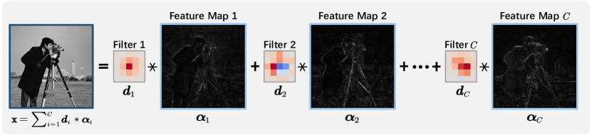
Figure 1: Illustration of the idea of convolutional coding. An image $\mathbf{x}$ is represented by the combination (sum) of multiple image-level convolution results, i.e., $\mathbf{x}=\sum_{i=1}^{C}\boldsymbol{d}_{i}\ast\boldsymbol{\alpha}_{i}$, where $\boldsymbol{d}_{i}\in\mathbb{R}^{k\times k}$ is the $i^{\mathrm{th}}$ dictionary filter, $\boldsymbol{\alpha}_{i}\in\mathbb{R}^{h\times w}$ is the $i^{\mathrm{th}}$ feature map, $\ast$ is the convolution operator and $C$ is the number of feature channels. The darker red (or blue) colors in each visualized filter correspond to the positive (or negative) entries with larger absolute values. Compared with the vanilla single-channel image data, this type of feature-level representation naturally enjoys higher capacity and flexibility.

Recently, convolutional coding methods have been successfully adopted in DUNs [30, 31, 32]. As shown in Fig. 1, through the convolutional coding model, an image $\mathbf{x}\in\mathbb{R}^{h\times w}$ is represented as $\mathbf{x}=\mathbf{D}\circledast\boldsymbol{\alpha}=\sum_{i=1}^{C}\boldsymbol{d}_{i}\ast\boldsymbol{\alpha}_{i}$, where $\ast$ is the 2D convolution operator and $C$ is the number of channels; $\mathbf{D}\in\mathbb{R}^{C\times k\times k}$ is the convolutional dictionary and $\boldsymbol{d}_{i}$ is the $i^{\mathrm{th}}$ dictionary filter; $\boldsymbol{\alpha}\in\mathbb{R}^{C\times h\times w}$ is the feature map of image $\mathbf{x}$ and $\boldsymbol{\alpha}_{i}$ is the $i^{\mathrm{th}}$ channel of $\boldsymbol{\alpha}$. Taking the natural advantage of $\boldsymbol{\alpha}$ being $C$-channel, these convolutional-coding-domain-based DUNs can transmit high-throughput information between stages. However, they only focus on specific tasks such as rain removal [31] and image denoising [32], lacking generalizability and flexibility.

To address the above issues, in this paper, we propose a Dual-Domain Deep Convolutional Coding Network, dubbed $\mathrm{D^{3}C^{2}}$-Net, focusing on CS reconstruction. Specifically, we design a novel dual-domain unfolding framework, which resolves the lack of generalizability of existing methods, allows our $\mathrm{D^{3}C^{2}}$-Net to transmit high-throughput information and inherits the advantages of image and convolutional-coding domain constraints. The proposed $\mathrm{D^{3}C^{2}}$-Net can be viewed as an attempt to bridge the gap between convolutional coding methods and neural networks in the CS reconstruction problem, with the merits of clear interpretability and sufficient information throughput.

Our main contributions are three-fold: (1) We propose a novel generalized dual-domain optimization framework, which integrates the merits of both image-domain and convolutional-coding-domain priors to constrain the feasible solution space and can be easily generalized to other image inverse problems. (2) We design a new Dual-Domain Deep Convolutional Coding Network ($\mathrm{D^{3}C^{2}}$-Net) for general CS reconstruction based on our proposed framework. Our $\mathrm{D^{3}C^{2}}$-Net can transmit high-throughput feature-level image representation through all unfolded stages to capture sufficient features adaptively, thus recovering more details and textures. (3) Experiments on natural and MR image CS tasks show that our $\mathrm{D^{3}C^{2}}$-Net outperforms existing state-of-the-art networks by large margins.

2 Related work

Deep unfolding network. Deep unfolding networks (DUNs) have been proposed to solve various image inverse problems [33, 34, 35, 32, 36, 37]. For CS and compressive sensing MRI (CS-MRI) tasks, DUNs usually combine convolutional neural network (CNN) denoisers with some optimization algorithms, like alternating minimization (AM) [38, 39, 40], half quadratic splitting (HQS) [41, 42, 43], iterative shrinkage-thresholding algorithm (ISTA) [44, 25, 26, 28], alternating direction method of multipliers (ADMM) [45] and inertial proximal algorithm for nonconvex optimization (iPiano) [46]. Although existing DUNs benefit from well-defined interpretability, their inherent design of image-domain-based unfolding limits the feature transmission capability. Some DUNs introduce intermediate results as auxiliary information to transmit between stages but do not change the idea of image-domain-based unfolding, which impairs performance improvement [47, 28].

Deep convolutional coding. Convolutional coding has been widely studied in image restoration [48, 49, 50]. Compared with traditional sparse coding methods, convolutional coding is shift-invariant and can flexibly represent the whole image. Nevertheless, most existing convolutional coding methods still use hand-crafted sparsity priors [30, 51, 52, 53], e.g., $\ell_{0}$-norm or $\ell_{1}$-norm, instead of learning complex priors from data, without exploiting the learning capability of deep neural networks. Recently, deep priors of convolutional coding have been integrated into deep unfolding methods. Wang et al. [31] designed an interpretable deep network for rain removal. Zheng et al. [32] proposed a deep convolutional dictionary learning framework for denoising. However, they only target the special cases where the measurement (or degradation) matrix $\mathbf{\Phi}$ in Eq. (1) is identity, i.e., $\mathbf{\Phi}=\mathbf{I}$.

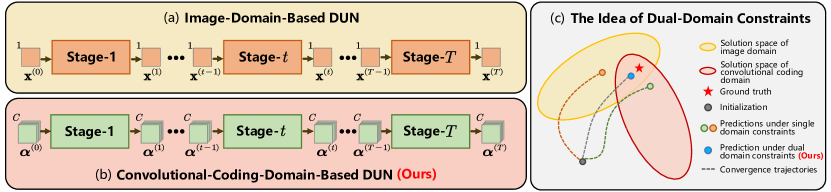
Figure 2: Illustration of the main ideas of dual-domain DUN design. (a) shows the architecture of the image-domain-based DUN and (b) shows the architecture of the convolutional-coding-domain-based DUN. Compared with (a) recovering the target image step-by-step ($\{\mathbf{x}^{(t)}\}$), our (b) transmits high-dimensional features ($\{\boldsymbol{\alpha}^{(t)}\}$) through all the unfolded stages. (c) further compares the converge trajectories under single and our dual-domain constraints, where the latter achieves more accurate recoveries than the former by employing the combination of learned dual-domain knowledges.

3 Proposed $\mathbf{D^{3}C^{2}}$-Net for compressive sensing

3.1 Convolutional-coding-inspired dual-domain formulation

As discussed above, different from existing image-domain-based DUNs, we draw inspiration from convolutional coding methods to enhance the information transmission capability. Figs. 2(a) and (b) show the architecture of the image-domain-based and convolutional-coding-domain-based DUN, respectively. One can observe that, the inherent design of image-domain-based DUNs that the one-channel image $\mathbf{x}$ in Eq. (1) is taken as input and output of each stage greatly hampers the information transmission capability. Differently, taking the natural advantage of feature maps $\boldsymbol{\alpha}$ being $C$ channel, convolutional-coding-based DUNs can transmit high-throughput information between stages. Notably, the prior term in Eq. (1) plays an essential role in reconstructing process because it can narrow the feasible region in the solution space. This idea leads to the integration of image-domain and convolutional-coding-domain priors as follows:

$$\min_{\mathbf{D},\mathbf{z},\boldsymbol{\alpha}}\frac{1}{2}\|\mathbf{\Phi}\mathbf{z}-\mathbf{y}\|_{2}^{2}+\frac{\mu_{\mathbf{z}}}{2}\|\mathbf{z}-\mathbf{D}\circledast\boldsymbol{\alpha}\|_{2}^{2}+\lambda\psi(\boldsymbol{\alpha})+\tau\phi(\mathbf{z}),$$ (2)

where $\mathbf{z}\in\mathbb{R}^{h\times w}$ is precisely an image, $\boldsymbol{\alpha}\in\mathbb{R}^{C\times h\times w}$ is the feature map, $\phi(\mathbf{z})$ and $\psi(\boldsymbol{\alpha})$ are prior terms of image domain and convolutional-coding domain respectively, and $\mu_{\mathbf{z}}$, $\lambda$ and $\tau$ are trade-off parameters. We illustrate the advantages of dual-domain priors in Fig. 2(c). One can observe that the introduction of dual-domain priors further constrains the feasible region in the solution space, leading to better reconstruction results than single-domain-based methods. Besides, compared with objective functions in [31] and [32] where the measurement matrix $\mathbf{\Phi}$ in $\mathbf{y}=\mathbf{\Phi}\mathbf{x}+\mathbf{n}$ is specially the identity matrix $\mathbf{I}$, our method is more flexible and generalizable, and can be extended to other cases.

3.2 Dual-domain optimization framework

To simplify the overall optimization process, we collaboratively learn a universal $\mathbf{D}$ and the other network components through end-to-end training and solve $\mathbf{z}$ and $\boldsymbol{\alpha}$ in Eq. (2) iteratively as follows:

$$\mathbf{z}^{(t)} =\operatorname*{argmin}_{\mathbf{z}}\frac{1}{2}\|\mathbf{\Phi}\mathbf{z}-\mathbf{y}\|_{2}^{2}+\frac{\mu_{\mathbf{z}}}{2}\|\mathbf{z}-\mathbf{D}\circledast\boldsymbol{\alpha}^{(t-1)}\|_{2}^{2}+\tau\phi(\mathbf{z}),$$ (3a)

$$\boldsymbol{\alpha}^{(t)} =\operatorname*{argmin}_{\boldsymbol{\alpha}}\frac{\mu_{\mathbf{z}}}{2}\|\mathbf{D}\circledast\boldsymbol{\alpha}-\mathbf{z}^{(t)}\|^{2}_{2}+\lambda\psi(\boldsymbol{\alpha}).$$ (3b)

Image-level optimization. The image-domain optimization and the convolutional-coding-domain optimization are decoupled into Eqs. (3a) and (3b), respectively. The $\mathbf{z}$-subproblem in Eq. (3a) can be solved through ISTA by iterating between the following two update steps:

$$\mathbf{r}^{(t)} =\mathcal{G}_{\mathrm{GDM}}\left(\boldsymbol{\alpha}^{(t-1)},\mathbf{z}^{(t-1)},\mathbf{D},\rho,\mu_{\mathbf{z}}\right)$$ (4a)

$$=\mathbf{z}^{(t-1)}-\rho\left(\mathbf{\Phi}^{\top}\left(\mathbf{\Phi}\mathbf{z}^{(t-1)}-\mathbf{y}\right)+\mu_{\mathbf{z}}\left(\mathbf{z}^{(t-1)}-\mathbf{D}\circledast\boldsymbol{\alpha}^{(t-1)}\right)\right),$$

$$\mathbf{z}^{(t)} =\mathcal{G}_{\mathrm{PMN}}(\mathbf{r}^{(t)})=\mathrm{prox}_{\tau\phi}(\mathbf{r}^{(t)})=\operatorname*{argmin}_{\mathbf{z}^{*}}\frac{1}{2}\|\mathbf{z}^{*}-\mathbf{r}^{(t)}\|_{2}^{2}+\tau\phi(\mathbf{z}^{*}),$$ (4b)

where $\mathcal{G}_{\mathrm{GDM}}$ and $\mathcal{G}_{\mathrm{PMN}}$ denote the gradient descent module (GDM) and proximal mapping network (PMN), respectively. Their structural details will be elaborated on in the next subsection.

Feature-level optimization. For the $\boldsymbol{\alpha}$-subproblem in Eq. (3b), where $\frac{\mu_{\mathbf{z}}}{2}\|\mathbf{D}\circledast\boldsymbol{\alpha}-\mathbf{z}^{(t)}\|_{2}^{2}$ is the data term, $\psi(\boldsymbol{\alpha})$ is the prior term, and $\lambda$ is a trade-off parameter. To separate the data term and the prior term, we apply the HQS algorithm, which tackles Eq. (3b) by introducing an auxiliary variable $\tilde{\boldsymbol{\alpha}}$, leading to the following objective function:

$$\min_{\boldsymbol{\alpha},\tilde{\boldsymbol{\alpha}}}\frac{\mu_{\mathbf{z}}}{2}\|\mathbf{D}\circledast\tilde{\boldsymbol{\alpha}}-\mathbf{z}^{(t)}\|_{2}^{2}+\lambda\psi(\boldsymbol{\alpha})+\frac{\mu_{\boldsymbol{\alpha}}}{2}\|\boldsymbol{\alpha}-\tilde{\boldsymbol{\alpha}}\|_{2}^{2},$$ (5)

where $\mu_{\boldsymbol{\alpha}}$ is the penalty parameter for the distance between $\boldsymbol{\alpha}$ and $\tilde{\boldsymbol{\alpha}}$. The above Eq. (5) can be also solved iteratively as follows:

$$\tilde{\boldsymbol{\alpha}}^{(t)} =\operatorname*{argmin}_{\boldsymbol{\alpha}^{*}}\frac{1}{2}\|\mathbf{D}\circledast\boldsymbol{\alpha}^{*}-\mathbf{z}^{(t)}\|_{2}^{2}+\frac{\eta}{2}\|\boldsymbol{\alpha}^{*}-\boldsymbol{\alpha}^{(t-1)}\|_{2}^{2},$$ (6a)

$$\boldsymbol{\alpha}^{(t)} =\operatorname*{argmin}_{\boldsymbol{\alpha}^{*}}\frac{1}{2}\|\boldsymbol{\alpha}^{*}-{\tilde{\boldsymbol{\alpha}}}^{(t)}\|_{2}^{2}+\beta\psi({\boldsymbol{\alpha}^{*}}),$$ (6b)

where $\eta={\mu_{\boldsymbol{\alpha}}}/{\mu_{\mathbf{z}}}$ and $\beta={\lambda}/{\mu_{\boldsymbol{\alpha}}}$. For solving the Eq. (6a), the Fast Fourier Transform (FFT) can be utilized by assuming the convolution is carried out with circular boundary conditions. Let $\mathbfcal{D}=\mathcal{F}(\mathbf{D})$, $\mathbfcal{Z}^{(t)}=\mathcal{F}(\mathbf{z}^{(t)})$, and $\mathbfcal{A}^{(t-1)}=\mathcal{F}(\boldsymbol{\alpha}^{(t-1)})$, where $\mathcal{F}(\cdot)$ denotes the 2D FFT. Following [32], we apply the data-term solving module (DTSM), leading the following closed-form solution:

$$\begin{split}\tilde{\boldsymbol{\alpha}}^{(t)}&=\mathcal{G}_{\mathrm{DTSM}}\left(\boldsymbol{\alpha}^{(t-1)},\mathbf{z}^{(t)},\mathbf{D},\eta\right)=\frac{1}{\eta}\mathcal{F}^{-1}\left(\mathbfcal{H}^{(t)}-\mathbfcal{D}\circ\left(\frac{\left(\mathbfcal{\bar{D}}\odot\mathbfcal{H}^{(t)}\right)}{\eta+\left(\mathbfcal{\bar{D}}\odot\mathbfcal{D}\right)}\uparrow_{C}\right)\right),\end{split}$$ (7)

where $\circ$ is the Hadamard product, $\mathbf{X}\odot\mathbf{Y}=\sum_{i=1}^{C}\mathbf{X}_{i}\circ\mathbf{Y}_{i}$, $\mathbf{X}\uparrow_{C}$ expands the channel dimension of $\mathbf{X}$ to $C$, $\div$ is the Hadamard division, $\mathcal{F}^{-1}(\cdot)$ denotes the inverse of FFT, $\mathbfcal{\bar{D}}$ denotes the complex conjugate of $\mathbfcal{D}$, and $\mathbfcal{H}^{(t)}$ is defined as $\mathbfcal{H}^{(t)}=\mathbfcal{D}\circ\left(\mathbfcal{Z}^{(t)}\uparrow_{C}\right)+\eta\mathbfcal{A}^{(t-1)}$.

For solving the Eq. (6b), we apply a prior-term solving network (PTSN) to estimate $\boldsymbol{\alpha}^{(t)}$ as follows:

$$\boldsymbol{\alpha}^{(t)}=\mathcal{G}_{\mathrm{PTSN}}\left(\tilde{\boldsymbol{\alpha}}^{(t)},\beta\right),$$ (8)

and the structural design of PTSN will be presented in the following.

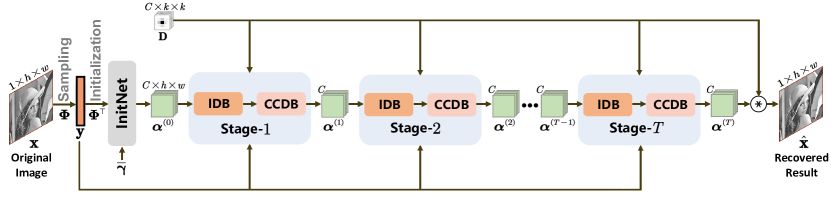
Figure 3: The overall architecture of our proposed $\mathrm{D^{3}C^{2}}$-Net with $T$ stages. Each stage consists of an image domain block (IDB) and a convolutional coding domain block (CCDB). $\mathbf{x}$ denotes the full-sampled image, $\mathbf{y}$ is the under-sampled data, and $\hat{\mathbf{x}}$ denotes the output of the $\mathrm{D^{3}C^{2}}$-Net. $\mathbf{D}$ is the convolutional dictionary, and $\boldsymbol{\alpha}$ is the feature map. $k$ denotes the filter size of $\mathbf{D}$, $h$ and $w$ denote the height and width of $\mathbf{x}$ and $\boldsymbol{\alpha}$, and $C$ is the number of channels.

3.3 $\mathbf{D^{3}C^{2}}$-Net unfolding architecture design

As discussed above, the unfolding optimization consists of an image-domain optimization subproblem (i.e., Eq. (3a)) and a convolutional-coding-domain optimization subproblem (i.e., Eq. (3b)). Mapping the unfolding process into a deep neural network, we propose our $\mathrm{D^{3}C^{2}}$-Net, which alternates between the image domain block (IDB) and the convolutional coding domain block (CCDB). Fig. 3 illustrates the overall architecture of $\mathrm{D^{3}C^{2}}$-Net with $T$ stages, whereby the recovered result $\hat{\mathbf{x}}$ is obtained by $\hat{\mathbf{x}}=\mathbf{D}\circledast\boldsymbol{\alpha}^{(T)}$. It can be seen that the proposed $\mathrm{D^{3}C^{2}}$-Net can transmit $C$-channel high-throughput information between every two adjacent stages. Fig. 4(a) gives more details about each stage. As shown in Fig. 4(a), each IDB is composed of a gradient descent module (GDM in Eq. (4a)) and a proximal mapping network (PMN in Eq. (4b)), while each CCDB is composed of a data-term solving module (DTSM in Eq. (7)) and a prior-term solving network (PTSN in Eq. (8)). Besides, for hyper-parameters $\left\{\rho,\mu_{\mathbf{z}},\eta,\beta\right\}$, inspired by [54] and [32], we adopt a hyper-parameter network (HPN) to predict them for each stage. Fig. 4(b) illustrates the architectures of the sub-networks, including InitNet, PMN, PTSN and HPN. More details are shown below.

InitNet takes the concatenation of $\mathbf{x}^{\mathrm{init}}$ and $\bar{\boldsymbol{\gamma}}$ as input to obtain a feature map initialization $\boldsymbol{\alpha}^{(0)}$, where $\mathbf{x}^{\mathrm{init}}=\mathbf{\Phi}^{\top}\mathbf{y}$, and $\bar{\boldsymbol{\gamma}}$ is the CS ratio map generated from $\gamma$ with a same dimension as $\mathbf{x}$. It consists of two convolutional layers ($\mathrm{Conv_{1}}(\cdot)$ and $\mathrm{Conv_{2}}(\cdot)$). The former one receives 2-channel inputs and generates $C$-channel outputs with ReLU activation. InitNet is formulated as:

$$\boldsymbol{\alpha}^{(0)}=\mathcal{G}_{\mathrm{InitNet}}\left(\mathbf{x}^{\mathrm{init}},\bar{\boldsymbol{\gamma}}\right)=\mathrm{Conv_{2}}(\mathrm{ReLU}(\mathrm{Conv_{1}}(\mathrm{Concat}(\mathbf{x}^{\mathrm{init}},\bar{\boldsymbol{\gamma}})))).$$ (9)

PMN solves the proximal mapping problem $\mathrm{prox}_{\tau\phi}(\mathbf{r}^{(t)})$. It consists of two convolutional layers ($\mathrm{Conv_{1}}(\cdot)$ and $\mathrm{Conv_{2}}(\cdot)$) and two residual blocks ($\mathrm{RB_{1}}(\cdot)$ and $\mathrm{RB_{2}}(\cdot)$), which generate residual outputs by the structure of Conv-ReLU-Conv. Specifically, $\mathrm{Conv_{1}}(\cdot)$ takes one-channel $\mathbf{r}^{(t)}$ as input and generates $C$-channel outputs. Then two $\mathrm{RB}(\cdot)$s are used to extract deep representation. Finally, $\mathrm{Conv_{2}}(\cdot)$ outputs the result by feature conversions from $C$-channel to one-channel under a residual learning strategy. Accordingly, PMN can be formulated as:

$$\mathbf{z}^{(t)}=\mathcal{G}_{\mathrm{PMN}}^{(t)}\left(\mathbf{r}^{(t)}\right)=\mathbf{r}^{(t)}+\mathrm{Conv_{2}}(\mathrm{RB_{2}}(\mathrm{RB_{1}}(\mathrm{Conv_{1}}(\mathbf{r}^{(t)})))).$$ (10)

PTSN takes the concatenation of $\tilde{\boldsymbol{\alpha}}^{(t)}$ and $\bar{\boldsymbol{\beta}}^{(t)}$ as input to learn the implicit prior on feature map $\boldsymbol{\alpha}$, where $\bar{\boldsymbol{\beta}}^{(t)}$ is generated from $\beta^{(t)}$ as $\bar{\boldsymbol{\gamma}}$ does. It consists of one convolutional layer ($\mathrm{Conv_{1}(\cdot)}$) and two residual blocks ($\mathrm{RB_{1}}(\cdot)$ and $\mathrm{RB_{2}}(\cdot)$). The convolutional layer receives $(C+1)$-channel inputs and generates $C$-channel outputs. Residual learning strategy is applied. PTSN is formulated as:

$$\boldsymbol{\alpha}^{(t)}=\mathcal{G}_{\mathrm{PTSN}}^{(t)}\left(\tilde{\boldsymbol{\alpha}}^{(t)},\bar{\boldsymbol{\beta}}^{(t)}\right)=\tilde{\boldsymbol{\alpha}}^{(t)}+\mathrm{RB_{2}}(\mathrm{RB_{1}}(\mathrm{Conv_{1}}(\mathrm{Concat}(\tilde{\boldsymbol{\alpha}}^{(t)},\bar{\boldsymbol{\beta}}^{(t)})))).$$ (11)

HPN takes CS ratio map $\bar{\boldsymbol{\gamma}}$ as input and predicts hyper-parameters for each stage. It consists of two $1\times 1$ convolutional layers with Sigmoid as the first activation function and Softplus as the last, ensuring all hyper-parameters are positive. HPN can be formulated as:

$$\left(\rho^{(t)},\mu_{\mathbf{z}}^{(t)},\eta^{(t)},\beta^{(t)}\right)=\mathcal{G}_{\mathrm{HPN}}^{(t)}\left(\bar{\boldsymbol{\gamma}}\right)=\mathrm{Softplus}(\mathrm{Conv_{2}}(\mathrm{Sigmoid}(\mathrm{Conv_{1}}(\bar{\boldsymbol{\gamma}})))).$$ (12)

To sum up, with jointly taking the sampling matrix $\mathbf{\Phi}$ and the recovery network as combined learnable parts, the collection of all parameters incorporated in $\mathrm{D^{3}C^{2}}$-Net, denoted by $\mathbf{\Theta}$, can be collaboratively learned and expressed as $\mathbf{\Theta}=\{\mathbf{\Phi},\mathbf{D},\mathcal{G}_{\mathrm{InitNet}}(\cdot)\}\cup\{\mathcal{G}_{\mathrm{PMN}}^{(t)}(\cdot),\mathcal{G}_{\mathrm{PTSN}}^{(t)}(\cdot),\mathcal{G}_{\mathrm{HPN}}^{(t)}(\cdot)\}_{t=1}^{T}$.

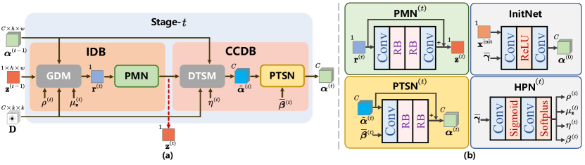
Figure 4: Illustration of the structural design of the unfolded stage and its components. (a) is the structure of $t$-th stage in $\mathrm{D^{3}C^{2}}$-Net. An image domain block (IDB) consists of a gradient descent module (GDM) and a proximal mapping network (PMN). A convolutional coding domain block (CCDB) consists of a data-term solving module (DTSM) and a prior-term solving network (PTSN). (b) shows the architectures of four sub-networks in each $\mathrm{D^{3}C^{2}}$-Net stage.

4 Experiments

4.1 Implementation details

Loss function. Given a set of full-sampled images $\{\mathbf{x}_{j}\}_{j=1}^{N_{a}}$ and CS ratio $\gamma$, the measurement is obtained by $\mathbf{y}_{j}=\mathbf{\Phi}\mathbf{x}_{j}$, yielding training data pairs $\{\mathbf{y}_{j},\mathbf{x}_{j}\}_{j=1}^{N_{a}}$. Our $\mathrm{D^{3}C^{2}}$-Net takes $\mathbf{y}_{j}$ as the input of its recovery network and outputs the reconstruction $\hat{\mathbf{x}}_{j}$ with the parameter-free initialization $\mathbf{x}^{\mathrm{init}}_{j}=\mathbf{\Phi}^{\top}\mathbf{y}_{j}$. Following [26, 29], we adopt the block-based CS sampling setup, where a high-dimensional image is divided into non-overlapping blocks and sampled independently, i.e., $\mathbf{x}_{j}$, $\mathbf{x}^{\mathrm{init}}_{j}$ and $\hat{\mathbf{x}}_{j}$ are tensors of size $1$$\times$$\sqrt{N}$$\times$$\sqrt{N}$. More details about sampling and initialization are provided in the supplementary materials. To reduce the discrepancy between $\mathbf{x}_{j}$ and $\hat{\mathbf{x}}_{j}$, an $\ell_{2}$ discrepancy loss is defined by the mean square error (MSE), i.e., $\mathcal{L}_{disc}=\frac{1}{NN_{a}}\sum_{j=1}^{N_{a}}\|\hat{\mathbf{x}}_{j}-\mathbf{x}_{j}\|_{F}^{2}$, where $N_{a}$ and $N$ represent the total number of training images and the size of each image, respectively. For the orthogonal constraint of the jointly learned sampling matrix $\mathbf{\Phi}$, the orthogonal loss term is designed as $\mathcal{L}_{orth}=\frac{1}{M^{2}}\|\mathbf{\Phi}\mathbf{\Phi}^{\top}-\mathbf{I}\|_{F}^{2}$. Therefore, the end-to-end loss for $\mathrm{D^{3}C^{2}}$-Net is defined as $\mathcal{L}(\mathbf{\Theta})=\mathcal{L}_{disc}+\xi\mathcal{L}_{orth}$, where $\xi$ is the regularization parameter, which is set to $0.01$ in experiments.

Training. We use the combination of BSD400 [55, 33], DIV2K training set [56], and WED [57] for training. Training data pairs ${\{(\mathbf{y}_{j},\mathbf{x}_{j})\}}_{j=1}^{N_{a}}$ are obtained by extracting the luminance component of each image block of size $32$$\times$$32$, i.e., $N=1024$. The data augmentation technique is applied to increase the data diversity. Our $\mathrm{D^{3}C^{2}}$-Net is implemented in PyTorch [58]. All the experiments are performed on one NVIDIA GeForce RTX 3090. The Adam optimizer is used for updating the learnable parameters. The batch size is set to 32, and we train the network for $2.8$$\times$$10^{5}$ iterations. The learning rate starts from $1$$\times$$10^{-4}$ and decays a factor by $0.1$ after $1.6$$\times$$10^{5}$ and $2.4$$\times$$10^{5}$ iterations. The default filter size $k$ of each dictionary filter is set to be 5, the number of feature maps $C$ is set to be 64, and the stage number $T$ is set to be 8. The number of filters in $\mathbf{D}$ is determined by the number of feature maps (i.e., same as $C$). The selection of $k$, $C$ and $T$ is discussed in Section 4.2.

4.2 Ablation study

In this section, we first discuss the selection of filter size $k$ of $\mathbf{D}$, the number of feature maps $C$, and the number of stages $T$. Then we investigate the contribution of each domain in our dual-domain network. All the experiments are performed with CS ratio $\gamma=30\%$.

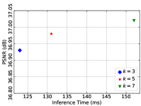
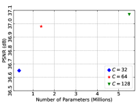
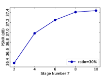
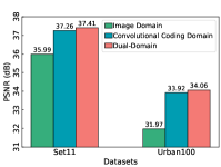
(a)	(b)	(c)	(d)

Figure 5: Ablation studies on (a) filter size $k$, (b) feature number $C$, (c) stage number $T$ and (d) effect of each domain. The experiments of (a), (b) and (c) are performed on the Set11 benchmark.

Dictionary filter size $k$. We first explore the effects of dictionary filter size $k\in\{3,5,7\}$. As shown in Fig. 5(a), the recovery performance is improved with a larger $k$ while the inference time increases. To balance the performance and efficiency, we choose $k=5$ in our default $\mathrm{D^{3}C^{2}}$-Net setting.

Number of feature maps $C$. We analyze the effect of $C\in\{32,64,128\}$. Fig. 5(b) provides the experimental comparison of PSNR and parameter number with different $C$s. With the increase of $C$, on the one hand, the throughput of $\mathrm{D^{3}C^{2}}$-Net improves, leading to better reconstruction performance. On the other hand, feature maps become redundant, resulting in huge network parameters and hard to be sufficiently trained. To get a better trade-off between reconstruction performance and the network computational complexity, we choose $C=64$ by default in $\mathrm{D^{3}C^{2}}$-Net.

Number of unfolded stages $T$. Since each $\mathrm{D^{3}C^{2}}$-Net stage corresponds to one iteration in our dual-domain unfolding framework, it is expected that a larger $T$ will lead to a higher reconstruction accuracy. Fig. 5(c) investigates the performances of five $\mathrm{D^{3}C^{2}}$-Net variants with $T\in\{2,4,6,8,10\}$. We observe that PSNR rises as $T$ increases, but the improvement becomes minor when $T\geq 8$. Considering the recovery accuracy-efficiency trade-offs, we employ $T=8$ in $\mathrm{D^{3}C^{2}}$-Net by default.

Effect of dual-domain constraints. To analyze the effectiveness of dual-domain priors, we compare our $\mathrm{D^{3}C^{2}}$-Net with two single-domain-based networks. A representative image-domain-only network OPINE-Net⁺ [26] is adopted for evaluation, each stage of which is similar to our IDB composed of a GDM and a PMN. To conduct a convolutional-coding-domain-only network, we remove the image-domain prior $\phi(\mathbf{z})$ in Eq. (3a), leading to the removal of PMN in $\mathrm{D^{3}C^{2}}$-Net for comparison. Fig. 5(d) shows the recovery performances of three different networks. It is clear to see that due to the enhancement of information transmission capability, the convolutional-coding-domain-only network boosts performance by 1.27dB on Set11 and 1.95dB on Urban100 over the image-domain-only network. Moreover, The combination of image and convolutional-coding domain priors (i.e., our default $\mathrm{D^{3}C^{2}}$-Net design) further improves the performance by about 0.15dB on both benchmarks, which demonstrates the effectiveness of dual-domain constraints.

4.3 Comparison with state-of-the-art methods

We compare our $\mathrm{D^{3}C^{2}}$-Net with five advanced CS methods, including CSNet⁺ [23], SCSNet [24], OPINE-Net⁺ [26], AMP-Net [59], and MADUN [28]. The average PSNR and SSIM reconstruction performance on Set11 [21] and Urban100 [60] datasets with respect to five CS ratios are summarized in Table 2. It can be observed that our $\mathrm{D^{3}C^{2}}$-Net outperforms all the other competing methods both in PSNR and SSIM under all given CS ratios, especially for lower ones. Fig. 6 further shows the visual comparison of two challenging images from Set11 and Urban100 datasets, respectively. As we can see, our $\mathrm{D^{3}C^{2}}$-Net recovers richer textures and details than all other methods.

Table 1: Parameter number (Millions) and recovery PSNR (dB) comparisons between MADUN and our $\mathrm{D^{3}C^{2}}$-Net on Urban100 dataset with $\gamma=10\%$.

Methods	#Param.	PSNR
MADUN [28]	3.13	26.23
$\mathrm{D^{3}C^{2}}$-Net (Ours)	2.72	27.54

Furthermore, we verify that the parameters in $\mathrm{D^{3}C^{2}}$-Net are used more rationally than MADUN [28], which directly introduces intermediate results as auxiliary information to transmit between stages without changing the idea of image-domain-based unfolding. As shown in Table 1, compared with MADUN, $\mathrm{D^{3}C^{2}}$-Net uses fewer parameters while improving PSNR by 1.31dB on Urban100 with $\gamma=10\%$, which validates the stronger learning capability of $\mathrm{D^{3}C^{2}}$-Net from our dual-domain unfolding principle.

Table 2: Average PSNR (dB) and SSIM performance comparisons on Set11 [21] and Urban100 [60] datasets with five different levels of CS ratios (or sampling rates). We compare our $\mathrm{D^{3}C^{2}}$-Net with five prior arts. The best and second best results are highlighted in red and blue colors, respectively.

Dataset	Methods	CS Ratio $\gamma$
		10%	20%	30%	40%	50%
Set11 [21]	CSNet+ [23]	28.34/0.8580	31.66/0.9203	34.30/0.9490	36.48/0.9644	38.52/0.9749
	SCSNet [24]	28.52/0.8616	31.82/0.9215	34.64/0.9511	36.92/0.9666	39.01/0.9769
	OPINE-Net+ [26]	29.81/0.8904	33.43/0.9392	35.99/0.9596	38.24/0.9718	40.19/0.9800
	AMP-Net [59]	29.40/0.8779	33.33/0.9345	36.03/0.9586	38.28/0.9715	40.34/0.9804
	MADUN [28]	29.89/0.8982	34.09/0.9478	36.90/0.9671	39.14/0.9769	40.75/0.9831
	$\mathrm{D^{3}C^{2}}$-Net (Ours)	30.80/0.9061	34.64/0.9512	37.41/0.9684	39.49/0.9773	41.29/0.9836
Urban100	CSNet+ [23]	23.96/0.7309	26.95/0.8449	29.12/0.8974	30.98/0.9273	32.76/0.9484
	SCSNet [24]	24.22/0.7394	27.09/0.8485	29.41/0.9016	31.38/0.9321	33.31/0.9534
	OPINE-Net+ [26]	25.90/0.7979	29.38/0.8902	31.97/0.9309	34.27/0.9548	36.28/0.9697
[60]	AMP-Net [59]	25.32/0.7747	29.01/0.8799	31.63/0.9248	33.88/0.9511	35.91/0.9673
	MADUN [28]	26.23/0.8250	30.24/0.9108	33.00/0.9457	35.10/0.9639	36.69/0.9746
	$\mathrm{D^{3}C^{2}}$-Net (Ours)	27.54/0.8464	30.98/0.9161	34.06/0.9522	36.11/0.9676	37.89/0.9771

Ground Truth	CSNet+	SCSNet	OPINE-Net+	AMP-Net	MADUN	$\mathrm{D^{3}C^{2}}$-Net
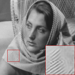
PSNR (dB)	31.22	31.43	32.92	33.53	35.02	37.04
PSNR (dB)	17.91	19.05	23.54	20.16	20.86	28.27

Figure 6: Visual comparisons on recovering an image named “Barbara” from Set11 [21] dataset with CS ratio $\gamma=30\%$ (top) and an image from Urban100 [60] dataset with CS ratio $\gamma=10\%$ (bottom).

4.4 Application to compressive sensing MRI

To demonstrate the generality of $\mathrm{D^{3}C^{2}}$-Net, we directly extend it to the practical problem of CS-MRI reconstruction, which aims at restoring MR images from a small number of under-sampled data in $k$-space. We follow the common practices in this application, setting the sampling matrix $\mathbf{\Phi}$ in Eq. (1) to $\mathbf{\Phi}=\mathbf{B}\mathbf{F}$, where $\mathbf{B}$ is an under-sampling matrix and $\mathbf{F}$ is the discrete Fourier transform. We follow MADUN [28] to use the same 100 fully sampled brain MR images as the training set. To avoid overfitting on this small data collection, we reduce the width and increase the depth of the network, yielding $\mathrm{D^{3}C^{2}}$-Net for MRI with $C=32$ and $T=20$, whose parameter number (1.72M) is fewer than $\mathrm{D^{3}C^{2}}$-Net for natural images (2.72M). The geometric data augmentation technique is also applied to increase the data diversity. As shown in Table 3, our $\mathrm{D^{3}C^{2}}$-Net outperforms the state-of-the-art methods on testing brain dataset under all given ratios. It is worth mentioning that due to the introduction of CS ratio information in InitNet and HPN, our $\mathrm{D^{3}C^{2}}$-Net for MRI is scalable for different ratios, i.e., it can handle five ratios by a single model, which significantly reduces the overall parameter number. Compared with MADUN (3.13M for each ratio), our $\mathrm{D^{3}C^{2}}$-Net leverages only about $\times\frac{1}{9}$ parameters while achieving better reconstruction performance on the CS-MRI task.

Table 3: Average PSNR/SSIM performance comparisons on testing brain MR images with eight recent methods. The best and second best results are highlighted in red and blue colors, respectively.

Methods	CS Ratio
	10%	20%	30%	40%	50%
Hyun et al. [20]	32.78/0.8385	36.36/0.9070	38.85/0.9383	40.65/0.9539	42.35/0.9662
Schlemper et al. [38]	34.23/0.8921	38.47/0.9457	40.85/0.9628	42.63/0.9724	44.19/0.9794
ADMM-Net [45]	34.42/0.8971	38.60/0.9478	40.87/0.9633	42.58/0.9726	44.19/0.9796
RDN [39]	34.59/0.8968	38.58/0.9470	40.82/0.9625	42.64/0.9723	44.18/0.9793
CDDN [40]	34.63/0.9002	38.59/0.9474	40.89/0.9633	42.59/0.9725	44.15/0.9795
ISTA-Net+ [25]	34.65/0.9038	38.67/0.9480	40.91/0.9631	42.65/0.9727	44.24/0.9798
MoDL [43]	35.18/0.9091	38.51/0.9457	40.97/0.9636	42.38/0.9705	44.20/0.9776
MADUN [28]	36.15/0.9237	39.44/0.9542	41.48/0.9666	43.06/0.9746	44.60/0.9810
$\mathrm{D^{3}C^{2}}$-Net (Ours)	36.48/0.9289	39.66/0.9558	41.59/0.9671	43.14/0.9748	44.63/0.9811

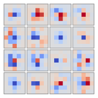
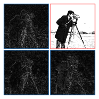
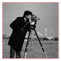
(a)	(b)	(c)	(d)

Figure 7: Visualizations for analyzing the learned dictionary $\mathbf{D}$ and feature maps $\boldsymbol{\alpha}$, including (a) learned global dictionary filters $\boldsymbol{d}_{i}$ in every four channels, whose values are distributed in $\left[-0.17,0.23\right]$, (b) feature maps $\boldsymbol{\alpha}_{9}$, $\boldsymbol{\alpha}_{25}$, $\boldsymbol{\alpha}_{41}$ and $\boldsymbol{\alpha}_{57}$, (c) low-frequency information $\boldsymbol{d}_{25}\ast\boldsymbol{\alpha}_{25}$ and the complementary (d) high-frequency information $\sum_{i\neq 25}\boldsymbol{d}_{i}\ast\boldsymbol{\alpha}_{i}$, with applying $\mathrm{D^{3}C^{2}}$-Net to the image named “Cameraman” from Set11 [21] with $\gamma=30\%$. $\mathrm{D^{3}C^{2}}$-Net learns diverse dictionary filters through end-to-end optimization with the recovery network trunk and obtains better image representations than prior arts with clearly separating the (c) low- and (d) high-frequency components.

4.5 Analysis of the learned dictionary $\mathbf{D}$ and feature map $\boldsymbol{\alpha}$

To further analyze the image representation capability of our $\mathrm{D^{3}C^{2}}$-Net, we visualize the learned convolutional dictionary $\mathbf{D}$ of the model and the final estimated feature maps on Set11 in the case of $\gamma=30\%$. Figs. 7(a) and (b) show some randomly picked dictionary filters $\boldsymbol{d}_{i}$ and feature maps $\boldsymbol{\alpha}_{i}$, respectively. It can be seen that our feature maps are not so sparse compared with those in convolutional sparse coding methods [30, 53] that explicitly impose sparsity priors. Interestingly, we observe that there is always one channel to preserve low-frequency information in our learned feature maps across the unfolded stage-by-stage inferences, e.g., the $25^{\mathrm{th}}$-channel shown in Fig. 7(b) with red border. We thus visualize $\boldsymbol{d}_{25}\ast\boldsymbol{\alpha}_{25}$ and its complementary $\sum_{i=1,i\neq 25}^{64}\boldsymbol{d}_{i}\ast\boldsymbol{\alpha}_{i}$ in Figs. 7(c) and (d), respectively. It is clear to see that our $\mathrm{D^{3}C^{2}}$-Net represents the image as the sum of one-layer low-frequency information and multi-layer high-frequency information through convolutional coding, which may make $\mathrm{D^{3}C^{2}}$-Net easier to keep and transmit high-frequency information among different stages in such a long trunk, thus achieving better reconstruction accuracies compared with prior arts.

5 Conclusion

Inspired by convolutional coding methods, we first propose a generalized dual-domain unfolding framework which combines the merits of both image-domain and convolutional-coding-domain priors to constrain the feasible region in the solution space. Compared with most existing convolutional coding methods, on the one hand, our framework adopts deep priors rather than traditional sparsity [30, 51, 52, 53] to better leverage the learning capability of deep neural networks. On the other hand, our framework is more generalizable, while existing deep convolutional coding methods for image restoration are exceptional cases where the degradation matrix $\mathbf{\Phi}$ is the identity $\mathbf{I}$ [31, 32]. Based on our proposed framework, we further design a novel Dual-Domain Deep Convolutional Coding Network for compressive sensing (CS) imaging, dubbed $\mathrm{D^{3}C^{2}}$-Net. Compared with most existing CS DUNs [25, 26, 27, 29], our $\mathrm{D^{3}C^{2}}$-Net transmits high-throughput feature-level representation through all stages and captures sufficient features adaptively. Extensive CS experiments on both natural and MR images demonstrate that $\mathrm{D^{3}C^{2}}$-Net outperforms state-of-the-art network-based CS methods with large accuracy margins and lower complexities. In the future, we will extend our generalizable unfolding framework and $\mathrm{D^{3}C^{2}}$-Net to more inverse imaging tasks and video applications.

References

- [1] Emmanuel J Candès, Justin Romberg, and Terence Tao. Robust uncertainty principles: Exact signal reconstruction from highly incomplete frequency information. IEEE Transactions on Information Theory, 52(2):489–509, 2006.
- [2] Richard G Baraniuk. Compressive sensing [lecture notes]. IEEE Signal Processing Magazine, 24(4):118–121, 2007.
- [3] Marco F Duarte, Mark A Davenport, Dharmpal Takhar, Jason N Laska, Ting Sun, Kevin F Kelly, and Richard G Baraniuk. Single-pixel imaging via compressive sampling. IEEE Signal Processing Magazine, 25(2):83–91, 2008.
- [4] Florian Rousset, Nicolas Ducros, Andrea Farina, Gianluca Valentini, Cosimo D’Andrea, and Françoise Peyrin. Adaptive basis scan by wavelet prediction for single-pixel imaging. IEEE Transactions on Computational Imaging, 3(1):36–46, 2016.
- [5] Michael Lustig, David Donoho, and John M Pauly. Sparse MRI: The application of compressed sensing for rapid mr imaging. Magnetic Resonance in Medicine: An Official Journal of the International Society for Magnetic Resonance in Medicine, 58(6):1182–1195, 2007.
- [6] Zhuoyuan Wu, Jian Zhang, and Chong Mou. Dense deep unfolding network with 3d-cnn prior for snapshot compressive imaging. Proceedings of the IEEE International Conference on Computer Vision (ICCV), 2021.
- [7] Zhuoyuan Wu, Zhenyu Zhang, Jiechong Song, and Jian Zhang. Spatial-temporal synergic prior driven unfolding network for snapshot compressive imaging. In Proceedings of IEEE International Conference on Multimedia and Expo (ICME), 2021.
- [8] Xuanyu Zhang, Yongbing Zhang, Ruiqin Xiong, Qilin Sun, and Jian Zhang. HerosNet: Hyperspectral explicable reconstruction and optimal sampling deep network for snapshot compressive imaging. Proceedings of the IEEE Conference on Computer Vision and Pattern Recognition (CVPR), 2022.
- [9] Jian Zhang, Debin Zhao, and Wen Gao. Group-based sparse representation for image restoration. IEEE Transactions on Image Processing, 23(8):3336–3351, 2014.
- [10] Jian Zhang, Chen Zhao, Debin Zhao, and Wen Gao. Image compressive sensing recovery using adaptively learned sparsifying basis via L0 minimization. Signal Processing, 103:114–126, 2014.
- [11] Yookyung Kim, Mariappan S Nadar, and Ali Bilgin. Compressed sensing using a Gaussian scale mixtures model in wavelet domain. In Proceedings of IEEE International Conference on Image Processing (ICIP), 2010.
- [12] Chen Zhao, Jian Zhang, Ronggang Wang, and Wen Gao. CREAM: CNN-regularized ADMM framework for compressive-sensed image reconstruction. IEEE Access, 6:76838–76853, 2018.
- [13] Christopher A Metzler, Arian Maleki, and Richard G Baraniuk. From denoising to compressed sensing. IEEE Transactions on Information Theory, 62(9):5117–5144, 2016.
- [14] Chen Zhao, Siwei Ma, and Wen Gao. Image compressive-sensing recovery using structured laplacian sparsity in DCT domain and multi-hypothesis prediction. In Proceedings of IEEE International Conference on Multimedia and Expo (ICME), 2014.
- [15] Chen Zhao, Siwei Ma, Jian Zhang, Ruiqin Xiong, and Wen Gao. Video compressive sensing reconstruction via reweighted residual sparsity. IEEE Transactions on Circuits and Systems for Video Technology, 27(6):1182–1195, 2016.
- [16] Chen Zhao, Jian Zhang, Siwei Ma, and Wen Gao. Nonconvex Lp nuclear norm based ADMM framework for compressed sensing. In Proceedings of the Data Compression Conference (DCC), 2016.
- [17] Chen Zhao, Jian Zhang, Siwei Ma, and Wen Gao. Compressive-sensed image coding via stripe-based DPCM. In Proceedings of the Data Compression Conference (DCC), 2016.
- [18] Ali Mousavi, Ankit B Patel, and Richard G Baraniuk. A deep learning approach to structured signal recovery. In Proceedings of the Annual Allerton Conference on Communication, Control, and Computing (Allerton), 2015.
- [19] Michael Iliadis, Leonidas Spinoulas, and Aggelos K Katsaggelos. Deep fully-connected networks for video compressive sensing. Digital Signal Processing, 72:9–18, 2018.
- [20] Chang Min Hyun, Hwa Pyung Kim, Sung Min Lee, Sungchul Lee, and Jin Keun Seo. Deep learning for undersampled MRI reconstruction. Physics in Medicine & Biology, 63(13):135007, 2018.
- [21] Kuldeep Kulkarni, Suhas Lohit, Pavan Turaga, Ronan Kerviche, and Amit Ashok. Reconnet: Non-iterative reconstruction of images from compressively sensed measurements. In Proceedings of the IEEE Conference on Computer Vision and Pattern Recognition (CVPR), 2016.
- [22] Yubao Sun, Jiwei Chen, Qingshan Liu, Bo Liu, and Guodong Guo. Dual-path attention network for compressed sensing image reconstruction. IEEE Transactions on Image Processing, 29:9482–9495, 2020.
- [23] Wuzhen Shi, Feng Jiang, Shaohui Liu, and Debin Zhao. Image compressed sensing using convolutional neural network. IEEE Transactions on Image Processing, 29:375–388, 2019.
- [24] Wuzhen Shi, Feng Jiang, Shaohui Liu, and Debin Zhao. Scalable convolutional neural network for image compressed sensing. In Proceedings of the IEEE Conference on Computer Vision and Pattern Recognition (CVPR), 2019.
- [25] Jian Zhang and Bernard Ghanem. ISTA-Net: Interpretable optimization-inspired deep network for image compressive sensing. In Proceedings of the IEEE Conference on Computer Vision and Pattern Recognition (CVPR), 2018.
- [26] Jian Zhang, Chen Zhao, and Wen Gao. Optimization-inspired compact deep compressive sensing. IEEE Journal of Selected Topics in Signal Processing, 14(4):765–774, 2020.
- [27] Di You, Jian Zhang, Jingfen Xie, Bin Chen, and Siwei Ma. COAST: Controllable arbitrary-sampling network for compressive sensing. IEEE Transactions on Image Processing, 30:6066–6080, 2021.
- [28] Jiechong Song, Bin Chen, and Jian Zhang. Memory-augmented deep unfolding network for compressive sensing. In Proceedings of the 29th ACM International Conference on Multimedia, 2021.
- [29] Di You, Jingfen Xie, and Jian Zhang. ISTA-Net++: flexible deep unfolding network for compressive sensing. In Proceedings of IEEE International Conference on Multimedia and Expo (ICME), 2021.
- [30] Xueyang Fu, Zheng-Jun Zha, Feng Wu, Xinghao Ding, and John Paisley. Jpeg artifacts reduction via deep convolutional sparse coding. In Proceedings of the IEEE Conference on Computer Vision and Pattern Recognition (CVPR), 2019.
- [31] Hong Wang, Qi Xie, Qian Zhao, and Deyu Meng. A model-driven deep neural network for single image rain removal. In Proceedings of the IEEE Conference on Computer Vision and Pattern Recognition (CVPR), 2020.
- [32] Hongyi Zheng, Hongwei Yong, and Lei Zhang. Deep convolutional dictionary learning for image denoising. In Proceedings of the IEEE Conference on Computer Vision and Pattern Recognition (CVPR), 2021.
- [33] Yunjin Chen and Thomas Pock. Trainable nonlinear reaction diffusion: A flexible framework for fast and effective image restoration. IEEE Transactions on Pattern Analysis and Machine Intelligence, 39(6):1256–1272, 2016.
- [34] Stamatios Lefkimmiatis. Non-local color image denoising with convolutional neural networks. In Proceedings of the IEEE Conference on Computer Vision and Pattern Recognition (CVPR), 2017.
- [35] Chris Metzler, Ali Mousavi, and Richard Baraniuk. Learned D-AMP: Principled neural network based compressive image recovery. In Proceedings of the International Conference on Neural Information Processing Systems (NeurIPS), 2017.
- [36] Jakob Kruse, Carsten Rother, and Uwe Schmidt. Learning to push the limits of efficient FFT-based image deconvolution. In Proceedings of the IEEE International Conference on Computer Vision (ICCV), 2017.
- [37] Filippos Kokkinos and Stamatios Lefkimmiatis. Deep image demosaicking using a cascade of convolutional residual denoising networks. In Proceedings of the European Conference on Computer Vision (ECCV), 2018.
- [38] Jo Schlemper, Jose Caballero, Joseph V Hajnal, Anthony N Price, and Daniel Rueckert. A deep cascade of convolutional neural networks for dynamic MR image reconstruction. IEEE Transactions on Medical Imaging, 37(2):491–503, 2017.
- [39] Liyan Sun, Zhiwen Fan, Yue Huang, Xinghao Ding, and John Paisley. Compressed sensing MRI using a recursive dilated network. In Proceedings of the Conference on Association for the Advancement of Artificial Intelligence (AAAI), 2018.
- [40] Hao Zheng, Faming Fang, and Guixu Zhang. Cascaded dilated dense network with two-step data consistency for MRI reconstruction. In Proceedings of the International Conference on Neural Information Processing Systems (NeurIPS), 2019.
- [41] Kai Zhang, Wangmeng Zuo, Shuhang Gu, and Lei Zhang. Learning deep CNN denoiser prior for image restoration. In Proceedings of the IEEE Conference on Computer Vision and Pattern Recognition (CVPR), 2017.
- [42] Weisheng Dong, Peiyao Wang, Wotao Yin, Guangming Shi, Fangfang Wu, and Xiaotong Lu. Denoising prior driven deep neural network for image restoration. IEEE Transactions on Pattern Analysis and Machine Intelligence, 41(10):2305–2318, 2018.
- [43] Hemant K Aggarwal, Merry P Mani, and Mathews Jacob. MoDL: Model-based deep learning architecture for inverse problems. IEEE Transactions on Medical Imaging, 38(2):394–405, 2018.
- [44] Davis Gilton, Greg Ongie, and Rebecca Willett. Neumann networks for linear inverse problems in imaging. IEEE Transactions on Computational Imaging, 6:328–343, 2019.
- [45] Yan Yang, Jian Sun, Huibin Li, and Zongben Xu. ADMM-CSNet: A deep learning approach for image compressive sensing. IEEE Transactions on Pattern Analysis and Machine Intelligence, 42(3):521–538, 2018.
- [46] Yueming Su and Qiusheng Lian. iPiano-Net: Nonconvex optimization inspired multi-scale reconstruction network for compressed sensing. Signal Processing: Image Communication, 89:115989, 2020.
- [47] Jiwei Chen, Yubao Sun, Qingshan Liu, and Rui Huang. Learning memory augmented cascading network for compressed sensing of images. In Proceedings of European Conference on Computer Vision (ECCV), 2020.
- [48] Shuhang Gu, Wangmeng Zuo, Qi Xie, Deyu Meng, Xiangchu Feng, and Lei Zhang. Convolutional sparse coding for image super-resolution. In Proceedings of the IEEE International Conference on Computer Vision (ICCV), 2015.
- [49] Xin Deng and Pier Luigi Dragotti. Deep convolutional neural network for multi-modal image restoration and fusion. IEEE Transactions on Pattern Analysis and Machine Intelligence, 43(10):3333–3348, 2020.
- [50] Minghan Li, Qi Xie, Qian Zhao, Wei Wei, Shuhang Gu, Jing Tao, and Deyu Meng. Video rain streak removal by multiscale convolutional sparse coding. In Proceedings of the IEEE Conference on Computer Vision and Pattern Recognition (CVPR), 2018.
- [51] Moran Xu, Dianlin Hu, Fulin Luo, Fenglin Liu, Shaoyu Wang, and Weiwen Wu. Limited-angle X-Ray CT reconstruction using image gradient -norm with dictionary learning. IEEE Transactions on Radiation and Plasma Medical Sciences, 5(1):78–87, 2020.
- [52] Hillel Sreter and Raja Giryes. Learned convolutional sparse coding. In Proceedings of the IEEE International Conference on Acoustics, Speech and Signal Processing (ICASSP), 2018.
- [53] Fangyuan Gao, Xin Deng, Mai Xu, Jingyi Xu, and Pier Luigi Dragotti. Multi-modal convolutional dictionary learning. IEEE Transactions on Image Processing, 2022.
- [54] Kai Zhang, Luc Van Gool, and Radu Timofte. Deep unfolding network for image super-resolution. In Proceedings of the IEEE Conference on Computer Vision and Pattern Recognition (CVPR), 2020.
- [55] David Martin, Charless Fowlkes, Doron Tal, and Jitendra Malik. A database of human segmented natural images and its application to evaluating segmentation algorithms and measuring ecological statistics. In Proceedings of the IEEE International Conference on Computer Vision (ICCV), 2001.
- [56] Radu Timofte, Eirikur Agustsson, Luc Van Gool, Ming-Hsuan Yang, and Lei Zhang. NTIRE 2017 challenge on single image super-resolution: Methods and results. In Proceedings of the IEEE Conference on Computer Vision and Pattern Recognition Workshops, 2017.
- [57] Kede Ma, Zhengfang Duanmu, Qingbo Wu, Zhou Wang, Hongwei Yong, Hongliang Li, and Lei Zhang. Waterloo exploration database: New challenges for image quality assessment models. IEEE Transactions on Image Processing, 26(2):1004–1016, 2016.
- [58] Adam Paszke, Sam Gross, Francisco Massa, Adam Lerer, James Bradbury, Gregory Chanan, Trevor Killeen, Zeming Lin, Natalia Gimelshein, Luca Antiga, et al. Pytorch: An imperative style, high-performance deep learning library. In Proceedings of the International Conference on Neural Information Processing Systems (NeurIPS), 2019.
- [59] Zhonghao Zhang, Yipeng Liu, Jiani Liu, Fei Wen, and Ce Zhu. AMP-Net: Denoising-based deep unfolding for compressive image sensing. IEEE Transactions on Image Processing, 30:1487–1500, 2020.
- [60] Jia-Bin Huang, Abhishek Singh, and Narendra Ahuja. Single image super-resolution from transformed self-exemplars. In Proceedings of the IEEE Conference on Computer Vision and Pattern Recognition (CVPR), 2015.