Exactly equivalent thermal conductivity in finite systems from equilibrium and nonequilibrium molecular dynamics simulations

Abstract

In a previous paper [Physical Review B 103, 035417 (2021)], we showed that the equilibrium molecular dynamics (EMD) method can be used to compute the apparent thermal conductivity of finite systems. It has been shown that the apparent thermal conductivity from EMD for a system with domain length $2L$ is equal to that from nonequilibrium molecular dynamics (NEMD) for a system with domain length $L$. Taking monolayer silicence with an accurate machine learning potential as an example, here we show that the thermal conductivity values from EMD and NEMD agree for the same domain length if the NEMD is applied with periodic boundary conditions in the transport direction. Our results thus establish an exact equivalence between EMD and NEMD for thermal conductivity calculations.

I Introduction

Molecular dynamics (MD) is one of the most important methods for studying heat transport at the nanoscale. The equilibrium MD (EMD) method based on the Green-Kubo relation Green (1954); Kubo (1957) and the nonequilibrium MD (NEMD) method based on a direct simulation of steady-state heat flow Ikeshoji and Hafskjold (1994); Müller-Plathe (1997); Jund and Jullien (1999); Shiomi (2014) are the two canonical methods for computing the lattice thermal conductivity in various materials. There have been extensive comparisons between the two methods for diffusive phonon transport Schelling et al. (2002); Sellan et al. (2010); He et al. (2012); Howell (2012); Dong et al. (2018) and it is now generally accepted Gu et al. (2021) that the two methods give consistent results in the diffusive limit.

While it has been believed that the EMD method can only be used to compute the thermal conductivity in the diffusive limit, we have recently shown Dong et al. (2021) that it can also be used to compute the apparent thermal conductivity (also called the effective thermal conductivity) of finite systems. For a finite system with nonperiodic boundary conditions applied to the transport direction, the running thermal conductivity (RTC) based on the Green-Kubo relation will eventually converges to zero in the limit of infinite-time, but it has been argued Dong et al. (2021) that the maximum value of the RTC can be interpreted as the apparent thermal conductivity of the finite system. However, it was found that the apparent thermal conductivity as computed from the EMD method for a system with domain length $2L$ is equal to that as computed from the NEMD method for a system with domain length $L$. This difference between the domain length is puzzling and in this work we show that it is related to the choice of simulation setups in the NEMD method: if the NEMD is performed with periodic boundary conditions, instead of fixed boundary conditions, in the transport direction, the thermal conductivity values from EMD and NEMD will agree for the same domain length. To be specific, our results are based on a case study of two-dimensional (2D) monolayer silicene using a recently developed machine learning potential Fan et al. (2021) that can accurately capture the phonon properties of this material.

II Models and Methods

II.1 The EMD simulation setup

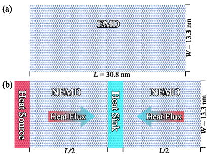
Figure 1: Schematic illustration of the EMD and NEMD simulation setups. (a) EMD simulation setup with open boundary conditions in the transport direction (horizontal) with domain length $L$. (b) NEMD simulation setup with periodic boundary conditions in the transport direction (horizontal). In NEMD, the heat source and sink are separated by $L/2$. In both EMD and NEMD, the transverse direction (vertical) has periodic boundary conditions and width $W$.

The EMD simulation setup considered in this paper is schematically illustrated in Fig. 1(a). To be specific, we align the zigzag direction of silicene in $x$ and the armchair direction in $y$ and study heat transport in the $x$ direction. Periodic boundary conditions are applied to the $y$ direction. In the $x$ direction, we use the free (open) boundary conditions to model a finite domain length $L$.

In the EMD method, after thermal equilibration, the system is evolved in the microcanonical ensemble and the equilibrium heat current Fan et al. (2015)

$$\vec{J}=\sum_{i}\sum_{j}\vec{r}_{ij}\frac{\partial U_{j}}{\partial\vec{r}_{ji}}\cdot\vec{v}_{i}$$ (1)

is sampled. Here, $U_{j}$ is the site potential of atom $j$, $\vec{v}_{i}$ is the velocity of atom $i$, and $\vec{r}_{ij}=-\vec{r}_{ji}=\vec{r}_{j}-\vec{r}_{i}$ is the relative position from atom $i$ to atom $j$. From the sampled heat current one can then calculate the heat current autocorrelation function (HCACF) $\langle J_{x}(0)J_{x}(t)\rangle$ and the RTC $\kappa(\tau)$ through the following Green-Kubo relation Green (1954); Kubo (1957):

$$\kappa(\tau)=\frac{1}{k_{\rm B}T^{2}V}\int_{0}^{\tau}\langle J_{x}(0)J_{x}(t)\rangle dt.$$ (2)

Here, $k_{\rm B}$ is Boltzmann’s constant, $T$ is the system temperature, and $V$ is the system volume.

II.2 The NEMD simulation setup

Figure 1(b) shows the NEMD simulation setup with periodic boundary conditions in the transport direction ($x$ direction). To be consistent with the EMD simulations, periodic boundary conditions are applied to the $y$ direction. In the $x$ direction, there are two thermostatted regions that are separated by $L/2$, serving as a heat source (with a higher temperature $T+\Delta T/2$) and a heat sink (with a lower temperature $T-\Delta T/2$). The total length of the parts without thermostat is thus $L$, which is the same as in the case of EMD. With a temperature difference of $\Delta T=20$ K, a typical temperature profile in the NEMD simulations is shown in Fig. 2(a).

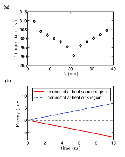
Figure 2: (a) Steady-state temperature profile and (b) energies of the thermostats coupled to the heat source and sink regions as a function of time in the NEMD simulation as shown in Fig. 1(b). The energy of the high-temperature thermostat decreases as it releases energy to the heat source region; the energy of the low-temperature thermostat increases as it absorbs energy from the heat sink region.

In the NEMD method, the heat source region will absorb energy from the high-temperature thermostat at a given rate $dE/dt$ when steady state is achieved. According to energy conservation, the heat sink region will simultaneously release energy to the low-temperature thermostat at the same rate, as shown in Fig. 2(b). Denoting the cross-sectional area as $A$, the heat flux in one direction shown in Fig. 1(b) is $dE/dt/(2A)$, where the factor $2$ accounts for the fact that the heat flows from the heat source region to the heat sink region via two opposite directions. Then, according to Fourier’s law, the apparent (effective) thermal conductivity $\kappa(L)$ of the finite system with domain length $L$ is

$$\kappa(L)=\frac{dE/dt/(2A)}{\Delta T/(L/2)},$$ (3)

Here the temperature gradient is taken as $\Delta T/(L/2)$, following the established practice Li et al. (2019); Hu et al. (2020).

II.3 Other MD simulation details

In both EMD and NEMD simulations, the width in the transverse direction is chosen as $W=13.3$ nm. The thickness of the monolayer silicene was chosen as the conventional value of $0.42$ nm Zhang et al. (2014); Dong et al. (2018); Zhang and Sun (2019); Fan et al. (2021). We consider the following domain lengths in the transport direction: $L$ = $7.7$, $15.4$, $30.8$, $61.6$, and $123.2$ nm.

For both EMD and NEMD simulations, we first equilibrate the system in the isothermal ensemble at $300$ K and zero pressure for $0.1$ ns. Then, in the EMD simulations, we evolve the system in the microcanonical ensemble for $5$ ns. In the NEMD simulations, we generate the nonequilibrium heat current using the local Langevin thermostats (with a coupling time of $0.1$ ps) for $10$ ns and use the second half of the data to compute the steady-state heat flux. We perform $30$ and $3$ independent runs for each domain length in the EMD and NEMD simulations, respectively. All the MD simulations are performed by using the open-source gpumd package Fan et al. (2013, 2017). A time step of $1$ fs is used in all the cases.

II.4 The NEP machine learning potential for silicene

We use the recently developed neuroevolution potential (NEP) Fan et al. (2021), which is a machine learning potential framework that can achieve high accuracy and low cost simultaneously.

The training data were obtained using an active learning scheme as implemented in the mlip package Novikov et al. (2021). We have considered temperatures ranging from $100$ to $900$ K and biaxial in-plane strains ranging from $-1\%$ to $1\%$. There are $914$ structures with $54840$ atoms in total. More details on the training data and the relevant hyperparameters in the NEP potential have been presented in Ref. Fan et al. (2021). The trained NEP potential as well as other inputs and outputs are freely available nep .

Figure 3(a) shows the evolution of the energy, force and virial root mean square errors (RMSEs) as a function of the number of generations during the training process. The predicted energy, force, and virial values from the trained NEP potential are compared with the reference values from quantum-mechanical density functional theory (DFT) calculations in Figs. 3(b)-3(d). The RMSEs for the energy, force components, and virial components are $1.5$ meV/atom, $56$ meV/Å, and $8.8$ meV/atom, respectively. These RMSEs are comparable to those obtained from other popular machine learning potentials but the NEP potential we use is much more computationally efficient Fan et al. (2021). For example, our NEP potential can achieve a speed of $1.3\times 10^{7}$ atom-step per second in MD simulations using a single Nvidia Tesla V100 GPU, while the moment tensor potential as implemented in mlip can only achieve a speed of $10^{5}$ atom-step per second using 72 Intel Xeon-Gold 6240 CPU cores. The efficiency of the NEP potential allows for doing large-scale and long-time MD simulations with a reasonable amount of computational resources.

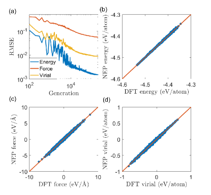
Figure 3: (a) Evolution of the energy, force, and virial RMSEs during the NEP training process. (b)-(d) The predicted energy, force, and virial values from the trained NEP potential as compared to the reference values from quantum-mechanical DFT calculations.

III Results and discussion

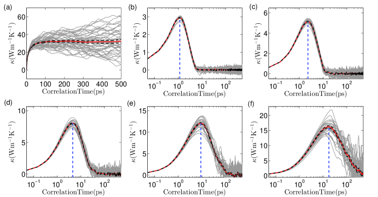
Figure 4: RTC $\kappa(\tau)$ as a function of the upper integration limit of the correlation time $\tau$ from EMD simulations with (a) periodic boundary conditions and (b)-(f) open boundary conditions in the transport direction. The domain lengths in (b)-(f) are $L$ = $7.7$, $15.4$, $30.8$, $61.6$, and $123.2$ nm. In each panel, the red thick line represents the mean value from the independent runs (the gray thin lines) and the black dashed lines indicate the error bounds. The blue dashed vertical lines in (b)-(f) correspond to the time $\tau_{\rm max}$ at which $\kappa(\tau)$ reaches a maximum.

Figure 4(a) shows the RTC $\kappa(\tau)$ of silicene as a function of the upper limit of the correlation time $\tau$ in the Green-Kubo integral. Here, periodic boundary conditions are applied to the transport direction and the simulated system can be considered as an infinite 2D system. In this case, the RTC will converge to a finite value which can be taken as the thermal conductivity of 2D silicene in the diffusive limit. We have used a sufficiently large domain size of $38.7$ $\times$ $40.2$ nm² with $24000$ atoms and the converged thermal conductivity is $31.9$ $\pm$ $1.4$ $\rm Wm^{-1}K^{-1}$, Which is consistent with the previous value ($33.7$ $\pm$ $0.6$ $\rm Wm^{-1}K^{-1}$) from the same NEP potential reported in Ref. Fan et al. (2021) as well as that ($32.4$ $\pm$ $2.9$ $\rm Wm^{-1}K^{-1}$) from a Gaussian approximation machine learning potential reported in Ref. Zhang and Sun (2019).

While the RTC converges to a finite value when periodic boundary conditions are applied in the transport direction, it always converges to zero when nonperiodic (open or fixed) boundary conditions are applied in the transport direction. This can be seen in Figs 4(b)-4(f) for all the domain lengths considered in this paper. Despite of the zero value in the infinite-time limit, the RTC in these finite systems exhibits a clear maximum value $\kappa^{\rm EMD}_{\rm max}$ at a particular correlation time $\tau_{\rm max}$. In our previous work Dong et al. (2021), this maximum value has been interpreted as the apparent thermal conductivity in the finite systems. Similar to Ref. Dong et al. (2021), we find that $\tau_{\rm max}$ is almost a linear function of the domain length $L$, $L\approx v_{\rm g}t_{\rm max}$, where the proportionality coefficient $v_{\rm g}$ can be interpreted as an effective group velocity of the phonons, which is fitted to be about $7$ km s^-1.

Table 1: Thermal conductivity data for finite systems with length ($L$) from the EMD ($\kappa^{\rm EMD}_{\rm max}$) and NEMD ($\kappa^{\rm NEMD}$) simulations.

$L$ (nm)	$\kappa^{\rm EMD}_{\rm max}$ ($\rm Wm^{-1}K^{-1}$)	$\kappa^{\rm NEMD}$ ($\rm Wm^{-1}K^{-1}$)
7.7	2.95$\pm$0.01	2.91$\pm$0.01
15.4	5.15$\pm$0.03	5.12$\pm$0.05
30.8	8.04$\pm$0.07	7.94$\pm$0.09
61.6	12.12$\pm$0.17	11.61$\pm$0.12
123.2	16.54$\pm$0.33	16.03$\pm$0.21

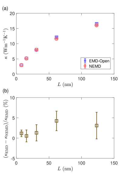
Figure 5: (a) The maximum thermal conductivity $\kappa_{\rm max}$ from EMD simulations with open boundary conditions in the transport direction and the apparent thermal conductivity from NEMD simulations as a function of the domain length $L$ for monolayer silicene at 300 K and zero pressure. (b) The relative difference of thermal conductivity between EMD and NEMD as a function of the domain length $L$.

The maximum RTC in EMD simulations with different $L$ are listed in Table 1. In this table, we also list the thermal conductivity values from NEMD simulations as calculated using Eq. (3). The data are also plotted in Fig. 5(a). It is clear that the thermal conductivity values from EMD and NEMD agree with each other excellently. As can be seen from Fig. 5(b), the relative difference of thermal conductivity between EMD and NEMD is less than $5\%$, which is comparable to the statistical uncertainty in the MD simulations. Mathematically, we have

$$\kappa^{\rm EMD}_{\rm max}(L)=\kappa^{\rm NEMD}(L).$$ (4)

Here we emphasize that the EMD results are obtained by using nonperiodic boundary conditions in the transport direction. We have used the open boundary conditions, but similar results can also be obtained by using fixed boundary conditions in the EMD simulations.

Different from Ref. Dong et al. (2021), where a relation $\kappa^{\rm EMD}_{\rm max}(2L)=\kappa^{\rm NEMD}(L)$ has been found, we do not have a difference of domain length between EMD and NEMD simulations in Eq. (4). This means that the EMD and NEMD simulation setups in Fig. 1 are directly comparable. Indeed, in both setups, the average phonon mean free paths related to phonon-boundary scattering are the same: in NEMD simulations, it is the separation of the two thermostats, which is $L/2$; in EMD simulations, it is the average path length between any point in the domain and a boundary, which is also $L/2$. It is this equivalence that gives rise to the same apparent thermal conductivity for a given domain length from the two methods.

While the two methods are equivalent in computing the apparent thermal conductivity in finite systems, they are not the methods of choice for computing the diffusive thermal conductivity in the infinite-length limit. Indeed, when $L=123.2$ nm, the apparent thermal conductivity is still only $16.03\pm 0.21$ $\rm Wm^{-1}K^{-1}$ from NEMD, which is only about one half of the diffusive thermal conductivity. However, at the nanoscale, one frequently needs to consider finite systems and the equivalence between EMD and NEMD demonstrated in this paper will be useful as one can choose the appropriate method that is more suitable for a particular application. One application that is more suitable for the EMD method is the determination of the apparent thermal conductivity of some zero-dimensional systems with irregular shapes, such as nanoparticles, in which case the application of the NEMD method is not very straightforward Matsubara et al. (2020).

IV Summary and Conclusions

In summary, we have calculated the apparent thermal conductivity of monolayer silicene with finite domain lengths based on an accurate NEP machine learning potential using EMD and NEMD methods. For a finite system of simulation domain length $L$, the maximum thermal conductivity $\kappa^{\rm EMD}_{\rm max}(L)$ from EMD simulations with open boundary conditions corresponds exactly to the apparent thermal conductivity $\kappa^{\rm NEMD}(L)$ from NEMD simulations with periodic boundary conditions in the transport direction. The EMD method with nonperiodic boundary conditions in the transport direction could be used in situations where the NEMD method is not straightforward to apply, such as characterizing the apparent thermal conductivity of finite nanoparticles.

References

- Green (1954) Melville S. Green, “Markoff random processes and the statistical mechanics of time-dependent phenomena. ii. irreversible processes in fluids,” The Journal of Chemical Physics 22, 398–413 (1954).
- Kubo (1957) Ryogo Kubo, “Statistical-mechanical theory of irreversible processes. i. general theory and simple applications to magnetic and conduction problems,” Journal of the Physical Society of Japan 12, 570–586 (1957).
- Ikeshoji and Hafskjold (1994) T. Ikeshoji and B. Hafskjold, “Non-equilibrium molecular dynamics calculation of heat conduction in liquid and through liquid-gas interface,” Molecular Physics 81, 251–261 (1994).
- Müller-Plathe (1997) Florian Müller-Plathe, “A simple nonequilibrium molecular dynamics method for calculating the thermal conductivity,” The Journal of Chemical Physics 106, 6082–6085 (1997).
- Jund and Jullien (1999) Philippe Jund and Rémi Jullien, “Molecular-dynamics calculation of the thermal conductivity of vitreous silica,” Phys. Rev. B 59, 13707–13711 (1999).
- Shiomi (2014) Junichiro Shiomi, “Nonequilirium molecular dynamics methods for lattice heat conduction calculations,” Annual Review of Heat Transfer 17, 177 (2014).
- Schelling et al. (2002) Patrick K. Schelling, Simon R. Phillpot, and Pawel Keblinski, “Comparison of atomic-level simulation methods for computing thermal conductivity,” Phys. Rev. B 65, 144306 (2002).
- Sellan et al. (2010) D. P. Sellan, E. S. Landry, J. E. Turney, A. J. H. McGaughey, and C. H. Amon, “Size effects in molecular dynamics thermal conductivity predictions,” Phys. Rev. B 81, 214305 (2010).
- He et al. (2012) Yuping He, Ivana Savic, Davide Donadio, and Giulia Galli, “Lattice thermal conductivity of semiconducting bulk materials: atomistic simulations,” Phys. Chem. Chem. Phys. 14, 16209–16222 (2012).
- Howell (2012) P. C. Howell, “Comparison of molecular dynamics methods and interatomic potentials for calculating the thermal conductivity of silicon,” The Journal of Chemical Physics 137, 224111 (2012).
- Dong et al. (2018) Haikuan Dong, Zheyong Fan, Libin Shi, Ari Harju, and Tapio Ala-Nissila, “Equivalence of the equilibrium and the nonequilibrium molecular dynamics methods for thermal conductivity calculations: From bulk to nanowire silicon,” Phys. Rev. B 97, 094305 (2018).
- Gu et al. (2021) Xiaokun Gu, Zheyong Fan, and Hua Bao, “Thermal conductivity prediction by atomistic simulation methods: Recent advances and detailed comparison,” Journal of Applied Physics 130, 210902 (2021).
- Dong et al. (2021) Haikuan Dong, Shiyun Xiong, Zheyong Fan, Ping Qian, Yanjing Su, and Tapio Ala-Nissila, “Interpretation of apparent thermal conductivity in finite systems from equilibrium molecular dynamics simulations,” Phys. Rev. B 103, 035417 (2021).
- Fan et al. (2021) Zheyong Fan, Zezhu Zeng, Cunzhi Zhang, Yanzhou Wang, Keke Song, Haikuan Dong, Yue Chen, and Tapio Ala-Nissila, “Neuroevolution machine learning potentials: Combining high accuracy and low cost in atomistic simulations and application to heat transport,” Phys. Rev. B 104, 104309 (2021).
- Fan et al. (2015) Zheyong Fan, Luiz Felipe C. Pereira, Hui-Qiong Wang, Jin-Cheng Zheng, Davide Donadio, and Ari Harju, “Force and heat current formulas for many-body potentials in molecular dynamics simulations with applications to thermal conductivity calculations,” Phys. Rev. B 92, 094301 (2015).
- Li et al. (2019) Zhen Li, Shiyun Xiong, Charles Sievers, Yue Hu, Zheyong Fan, Ning Wei, Hua Bao, Shunda Chen, Davide Donadio, and Tapio Ala-Nissila, “Influence of thermostatting on nonequilibrium molecular dynamics simulations of heat conduction in solids,” The Journal of Chemical Physics 151, 234105 (2019).
- Hu et al. (2020) Yue Hu, Tianli Feng, Xiaokun Gu, Zheyong Fan, Xufeng Wang, Mark Lundstrom, Som S. Shrestha, and Hua Bao, “Unification of nonequilibrium molecular dynamics and the mode-resolved phonon boltzmann equation for thermal transport simulations,” Phys. Rev. B 101, 155308 (2020).
- Zhang et al. (2014) Xiaoliang Zhang, Han Xie, Ming Hu, Hua Bao, Shengying Yue, Guangzhao Qin, and Gang Su, “Thermal conductivity of silicene calculated using an optimized stillinger-weber potential,” Phys. Rev. B 89, 054310 (2014).
- Zhang and Sun (2019) Cunzhi Zhang and Qiang Sun, “Gaussian approximation potential for studying the thermal conductivity of silicene,” Journal of Applied Physics 126, 105103 (2019).
- Fan et al. (2013) Zheyong Fan, Topi Siro, and Ari Harju, “Accelerated molecular dynamics force evaluation on graphics processing units for thermal conductivity calculations,” Computer Physics Communications 184, 1414 – 1425 (2013).
- Fan et al. (2017) Zheyong Fan, Wei Chen, Ville Vierimaa, and Ari Harju, “Efficient molecular dynamics simulations with many-body potentials on graphics processing units,” Computer Physics Communications 218, 10 – 16 (2017).
- Novikov et al. (2021) Ivan S Novikov, Konstantin Gubaev, Evgeny V Podryabinkin, and Alexander V Shapeev, “The MLIP package: moment tensor potentials with MPI and active learning,” Machine Learning: Science and Technology 2, 025002 (2021).
- (23) https://gitlab.com/brucefan1983/nep-data.
- Matsubara et al. (2020) Hiroki Matsubara, Gota Kikugawa, Takeshi Bessho, and Taku Ohara, “Evaluation of thermal conductivity and its structural dependence of a single nanodiamond using molecular dynamics simulation,” Diamond and Related Materials 102, 107669 (2020).