Effective operators
on an attractive magnetic edge

Abstract.

The semiclassical Laplacian with discontinuous magnetic field is considered in two dimensions. The magnetic field is sign changing with exactly two distinct values and is discontinuous along a smooth closed curve, thereby producing an attractive magnetic edge. Various accurate spectral asymptotics are established by means of a dimensional reduction involving a microlocal phase space localization allowing to deal with the discontinuity of the field.

1. Introduction

1.1. General framework

In this article, we consider the magnetic Laplacian on the plane $\mathbb{R}^{2}$,

(1.1) $$\mathcal{P}^{a}_{h}:=(-ih\nabla+\mathbf{A})^{2}=\sum_{j=1}^{2}(-ih\partial_{x_{j}}+A_{j})^{2},$$

with magnetic potential $\mathbf{A}:=(A_{1},A_{2})\in H^{1}_{\textrm{loc}}(\mathbb{R}^{2};\mathbb{R}^{2})$, generating the piecewise constant magnetic field

(1.2) $$B=\mathbf{1}_{\Omega_{1}}+a\mathbf{1}_{\Omega_{2}}\,,$$

where $-1\leqslant a\leqslant a_{0}$ and $a_{0}$ is a fixed negative constant. Here $h>0$ is a small parameter (the semiclassical parameter). Throughout this paper, we assume that

(1.3) $$\left\{\,\begin{aligned} \Omega_{1}\subset\mathbb{R}^{2}\text{ is a }&\text{connected and simply connected open set,}\leavevmode\nobreak\ \Omega_{2}=\mathbb{R}^{2}\setminus\overline{\Omega}_{1},\\ &\Gamma:=\partial\Omega_{1}\text{ is a }C^{\infty}\text{ smooth closed curve.}\\ \end{aligned}\,\right\}$$

and we refer to $\Gamma$ as the magnetic edge (see Fig 1). We will denote the length of $\Gamma$ by $|\Gamma|=2L$.

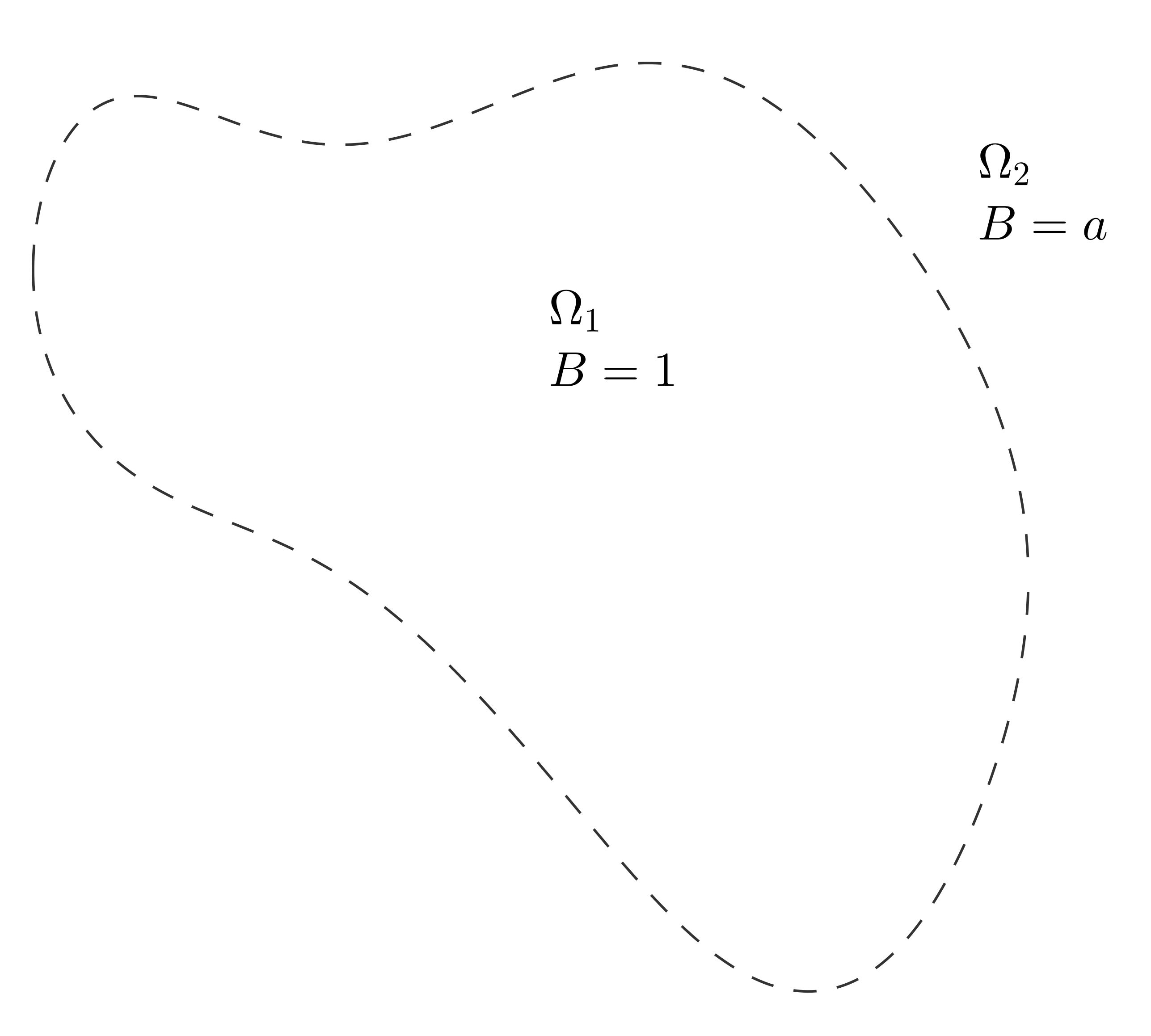
Figure 1. The plane $\mathbb{R}^{2}=\Omega_{1}\cup\Omega_{2}\cup\Gamma$ with the edge $\Gamma=\partial\Omega_{1}$ dashed.

The operator $\mathcal{P}^{a}_{h}$ is self-adjoint in $L^{2}(\mathbb{R}^{2})$ with domain

(1.4) $$\textsf{ Dom}(\mathcal{P}^{a}_{h})=\{u\in L^{2}(\mathbb{R}^{2})\leavevmode\nobreak\ :\leavevmode\nobreak\ (-ih\nabla+\mathbf{A})^{j}u\in L^{2}(\mathbb{R}^{2}),\leavevmode\nobreak\ j=1,2\}.$$

Its essential spectrum is determined by the magnetic field at infinity (in our case it is equal to $a$). More precisely, by Persson’s lemma, we have

$$\inf\mathrm{sp}_{\textrm{ess}}(\mathcal{P}^{a}_{h})\geqslant|a|h\,.$$

The purpose of this paper is to study the spectrum of $\mathcal{P}^{a}_{h}$ in the energy window $J_{h}=[0,Eh]$ with $E\in(0,|a|)$ a fixed constant (thus, we analyse the spectrum below the essential spectrum) and in the semiclassical limit $h\to 0$. We denote by $\lambda_{n}(\mathcal{P}^{a}_{h})$ the $n$’th eigenvalue of $\mathcal{P}^{a}_{h}$, and have

(1.5) $$\mathrm{sp}(\mathcal{P}^{a}_{h})\cap[0,Eh]=\{\lambda_{n}(\mathcal{P}^{a}_{h})\}_{n=1}^{N},$$

with $N=N(h)$.

Let us stress that our spectral analysis will be uniform with respect to $a\in[-1,a_{0}]$ and that the condition on the sign of $a$ is crucial since we will see that it implies a localization of the eigenfunctions associated with eigenvalues in $J_{h}$ near the edge $\Gamma$. That is why we will say that the edge is attractive.

1.2. Heuristics, earlier results, and motivation

1.2.1. Analogy with an electric well and mini-wells

The problem investigated in this paper shares common features with the semiclassical asymptotics of the Schrödinger operator, $-h^{2}\Delta+V$, with an electric potential $V$, in the full plane, see [17, 18, 25, 19]. In this context, the “well” is the set $\Gamma_{V}:=\{x\in\mathbb{R}^{2}\,|\,V(x)=\min_{\mathbb{R}^{2}}V\}$, which attracts the bound states in the limit $h\to 0$. The well is said to be non-degenerate if $\Gamma_{V}$ is a regular manifold, in which case the bound states might be localized near some points of $\Gamma_{V}$, the mini-wells. This phenomenon of mini-wells is a manifestation of a multi-scale localization of the bound states. Interestingly, this phenomenon occurs also in the setting of the magnetic Laplacian, with a Neumann boundary condition, or with a magnetic field having a step-discontinuity as in the present article. In particular, if we consider the Neumann Laplacian with a constant magnetic field in a bounded, smooth domain, the boundary of the domain acts as the “well” and the set of points of the boundary with maximum curvature acts as the “mini-well” (see [16, 9]).

1.2.2. Some known results

Recently in [1, 2], the operator $\mathcal{P}^{a}_{h}$ was considered in $L^{2}(\Omega)$ with Dirichlet boundary condition on $\partial\Omega$, $\Omega_{1}\subset\Omega$ and $\Gamma$ a smooth curve that meets $\partial\Omega$ transversely. The edge $\Gamma$ acts as the “well” and the set of points of $\Gamma$ with maximum curvature acts as the “mini-well”. Moreover, when the curvature has a unique non-degenerate maximum along the edge $\Gamma$, an accurate eigenvalue asymptotics displaying the splitting of the individual eigenvalues of $\mathcal{P}^{a}_{h}$ has been derived in [1, Thm. 1.2], when $-1<a<0$. This result is clearly reminiscent of [9].

1.2.3. Motivation

In the present article, we propose another perspective on the problem. Our spectral analysis will be uniform in various ways. Firstly, it will allow to derive, given some $E\in(0,|a|)$, an effective operator in the whole energy window $J_{h}=[0,Eh]$ with $h\in(0,h_{0}]$. In particular, the same strategy will provide us with Weyl estimates (estimating the number of eigenvalues in $J_{h}$) and the behavior of the individual eigenvalues. Secondly, it will also be uniform with respect to the parameter $a\in[-1,a_{0}]$. This uniformity is the key to the understanding of the transition between the regimes $a\in(-1,0)$ and $a=-1$. This is all the more motivating since the mini-well phenomenon does not occur when $a=-1$. It is indeed rather satisfactory to have a point of view encompassing quite different phenomena and showing their unity.

1.3. The band functions

The statement of our main results involves a family of 1D Schr$\ddot{\rm o}$dinger operators and their lowest eigenvalues, namely the operators obtained when the magnetic step is along a straight line, in which case a dimensional reduction is possible. This family has been the object of recent works (see [2, 20]). Let us briefly recall some of its basic properties. Straightening the edge $\Gamma$ locally, it is natural to consider the following “tangent” operator on $\mathbb{R}^{2}$ with magnetic field

$$B=\textrm{ curl\,}\mathbf{A}=\mathbf{1}_{\mathbb{R}_{+}\times\mathbb{R}}+a\mathbf{1}_{\mathbb{R}_{-}\times\mathbb{R}}\,,$$

where $a\in[-1,a_{0}]$ is a fixed constant. This operator is explicitely given by

(1.6) $$\mathcal{P}^{\mathrm{tgt}}_{h}=h^{2}D_{t}^{2}+(hD_{s}-tb_{a}(t))^{2}\,,\quad b_{a}(t)=\mathbf{1}_{\mathbb{R}_{+}}(t)+a\mathbf{1}_{\mathbb{R}_{-}}(t)\,.$$

By using a rescaling and a partial Fourier transformation along the straight edge $t=0$, we are led to consider the analytic family of Schrödinger operators

(1.7) $$\mathfrak{h}_{a}[\sigma]=-\partial^{2}_{t}+\big{(}\sigma-b_{a}(t)t\big{)}^{2}\,,$$

with domain

$$B^{2}(\mathbb{R})=\{u\in L^{2}(\mathbb{R}):u^{\prime\prime}\in L^{2}(\mathbb{R})\,,t^{2}u\in L^{2}(\mathbb{R})\}\,,$$

where $\sigma\in\mathbb{R}$ is a parameter.
The operator $\mathfrak{h}_{a}[\sigma]$ is self-adjoint in $L^{2}(\mathbb{R})$ and has compact resolvent. We denote by $(\mu^{[n]}_{a}(\sigma))_{n\geqslant 1}$ the non-decreasing sequence of the eigenvalues (repeated according to their multiplicity) of $\mathfrak{h}_{a}[\sigma]$. For shortness, we let

(1.8) $$\mu_{a}(\sigma)=\mu^{[1]}_{a}(\sigma)=\inf\mathrm{sp}(\mathfrak{h}_{a}[\sigma])\,.$$

By the Sturm-Liouville theory, we have the following proposition.

Proposition 1.1.

All the eigenvalues of $\mathfrak{h}_{a}[\sigma]$ are simple. The eigenfunction associated with $\mu^{[n]}_{a}(\sigma)$ has exactly $n-1$ simple zeroes on $\mathbb{R}$.

The functions $\mu^{[n]}_{a}(\sigma)$, are called the band functions. When $a=1$, we are reduced to the harmonic oscillator and $\mu^{[n]}_{a}(\sigma)=2n-1$. When $-1\leqslant a<1$, the functions $\mu^{[n]}_{a}(\sigma)$ are no more constant functions, see [20]. The lowest band function, $\mu_{a}(\sigma)$ is studied in [2].

Proposition 1.2 ([2, 20]).

For all $n\geqslant 1$, the function $\mu^{[n]}_{a}$ is analytic as a function of $\sigma$. Moreover, the lowest band function satisfies

(1.9) $$\lim\limits_{\sigma\to-\infty}\mu_{a}(\sigma)=+\infty,\quad\lim\limits_{\sigma\to+\infty}\mu_{a}(\sigma)=|a|\,,$$

and $\mu_{a}$ has a unique critical point, which is a non-degenerate minimum $\beta_{a}\in(0,|a|)$, attained at $\sigma(a)>0$.

In light of Proposition 1.2, we write, for $E\in(0,|a|)$,

(1.10) $$\mu^{-1}_{a}([\beta_{a},E])=\big{[}\sigma_{-}(a,E),\sigma_{+}(a,E)\big{]}\,,$$

where $-\infty<\sigma_{-}(a,E)<\sigma(a)<\sigma_{+}(a,E)<+\infty$.

1.4. Main results

Our analysis will reveal that the semiclassical spectral asymptotics of $\mathcal{P}^{a}_{h}$ in the interval $[0,Eh]$ is governed by that of an effective operator acting on the edge $\Gamma$. In particular, we obtain accurate asymptotics for the low-lying eigenvalues of $\mathcal{P}^{a}_{h}$ highlighting a significant difference between the cases where $-1<a<0$ and $a=-1$.

Theorem 1.3 (Case $-1<a<0$).

Assume that $k$ has a unique maximum, which is non-degenerate:

$$k_{max}:=\max_{\Gamma}k=k(s_{\max})\,,\quad k^{\prime\prime}(s_{\max})<0\,.$$

For all $a\in(-1,0)$, there exists $C(a)>0$ such that, for all $n\geqslant 1$,

$$\lambda_{n}(\mathcal{P}^{a}_{h})=\beta_{a}h-C(a)k_{\max}h^{\frac{3}{2}}+(n-\frac{1}{2})h^{\frac{7}{4}}\sqrt{-C(a)\mu^{\prime\prime}_{a}(\sigma(a))k^{\prime\prime}(s_{\max})}+o_{n}(h^{\frac{7}{4}})\,.$$

Remark 1.4.

1. Theorem 1.3 recovers the asymptotics obtained in [1]. The constant is given by $C(a)=-M_{3}(a)>0$, with $M_{3}(a)$ defined in (2.2) and calculated in (2.5).

2. The asymptotics in Theorem 1.3 is consistent with the phenomenon observed in surface superconductivity (see [9] and references therein) and the semiclassical analysis for the Schrödinger operator with a degenerate well in [18]. In this comparison, the well corresponds here to $\Gamma$ and the mini-wells correspond to the points of maximal curvature.

3. Actually, the proof of Theorem 1.3 provides us with a uniform description of the spectrum in $[0,Eh]$ and could also help determining the behavior of the eigenvalues close to $Eh$ when $E$ is non-critical for $\mu_{a}$, i.e., when $E\neq\beta_{a}$. In the context of the Robin Laplacian, such considerations are the object of the ongoing work [8]. Note also that there are some results high up in the spectrum in the recent work [15], where Dirichlet conditions are considered.

4. It might happen that $k$ does not have a unique minimum and even that $\Gamma$ has some symmetry properties. In this case, tunneling occurs and the eigenvalue splitting is exponentially small (see [11]). The proof is similar to the case of the Laplacian with a constant magnetic field and Neumann boundary condition in a symmetric domain [7].

When $a=-1$, we will prove that $C(a)=0$ and thus the second and third terms in the asymptotics formally vanish. We still get accurate estimates for the low-lying eigenvalues of $\mathcal{P}^{a}_{h}$ when $a=-1$, which involves an operator on the edge $\Gamma\simeq[-L,L)$, whose half-length is denoted by $L$.

Theorem 1.5 (Case $a=-1$).

There exists $C_{0}<0$ such that, for every $n\in\mathbb{N}$, we have as $h\to 0$,

$$\lambda_{n}(\mathcal{P}_{h}^{\{a=-1\}})=\beta_{-1}h+h^{2}\gamma_{n}(h)+o_{n}(h^{2})\,,$$

where $\gamma_{n}(h)$ is the non-decreasing sequence of the eigenvalues of the differential operator

$$\frac{\mu^{\prime\prime}_{-1}(\sigma(-1))}{2}\left(D_{s}+\alpha_{h}\right)^{2}+C_{0}k(s)^{2}\,,\quad\mbox{ with }D_{s}=-i\partial_{s}\,,$$

acting on $[-L,L)$ with periodic boundary conditions, and

(1.11) $$\alpha_{h}:=\frac{|\Omega_{1}|}{2Lh}-\frac{\sigma(-1)}{\sqrt{h}}\,.$$

Here $|\Omega_{1}|$ is the area of $\Omega_{1}$.

The quantity $\alpha_{h}$ in (1.11) involves the circulation of the magnetic potential along $\Gamma$. In fact, by Stokes’ Theorem, the circulation satisfies

$$\frac{1}{|\Gamma|}\int_{\Gamma}\mathbf{A}\cdot\tau\,\mathrm{d}s(x)=\frac{1}{|\Gamma|}\int_{\Omega_{1}}{\rm curl\,}\mathbf{A}\,\mathrm{d}x=\frac{|\Omega_{1}|}{2L}.$$

At the first glance, Theorems 1.3 and 1.5 seem independent. However, they both result from the analysis of the effective operator of $\mathcal{P}_{h}^{a}$ (see Theorem 1.6 below), which provides us with an accurate spectral description for $-1\leqslant a<0$.

This effective operator can be described as an $\hbar$-pseudodifferential operator on $\mathbb{R}$ with a $2L$-periodic symbol with respect to the space variable, and acting on $2L$-periodic functions. Here and along the whole paper the parameter

(1.12) $$\hbar:=h^{1/2}$$

is called the effective semiclassical parameter. Let us describe the shape of our effective operator. For a given symbol $p_{\hbar}(s,\sigma)\in S_{\mathbb{R}^{2}}(1)$ , we consider the Weyl quantization, i.e., the operator defined by

(1.13) $$({\rm Op}_{\hbar}^{w}(p_{\hbar})u)(s)=\frac{1}{2\pi\hbar}\int_{\mathbb{R}^{2}}e^{i(s-\tilde{s})\cdot\sigma/\hbar}p_{\hbar}\left(\frac{s+\tilde{s}}{2},\sigma\right)u(\tilde{s})\mathrm{d}\tilde{s}\mathrm{d}\sigma\,.$$

For an introduction to pseudo-differential operators, the reader is referred for instance to [26], where rigorous definitions are given and several fundamental properties are established. These operators being well defined on $\mathcal{S}(\mathbb{R})$, they can be extended by duality as operators on $\mathcal{S}^{\prime}(\mathbb{R})$. We now underline that, if $p_{\hbar}(s+2L,\sigma)=p_{\hbar}(s,\sigma)$, then ${\rm Op}_{\hbar}^{w}(p_{\hbar})$ transforms all the $2L$-periodic distributions into $2L$-periodic distributions. In fact, ${\rm Op}_{\hbar}^{w}(p_{\hbar})$ also preserves the space of $2L$-periodic functions that are in $L^{2}_{\rm{loc}}$, denoted by $L^{2}_{2L}(\mathbb{R})$ (see Section 4.1).

Such an induced operator will give us our effective operator and we will call it a pseudodifferential operator on the edge, $s$ representing the coordinate on $\Gamma$ (parametrised by arc-length).

The main result in this article is the following.

Theorem 1.6 (Spectral reduction to the edge).

There exists a self-adjoint $\hbar$-pseudodifferential operator (with symbol $p_{\hbar}^{\mathrm{eff}}\in S_{\mathbb{R}^{2}}(1)$) on the edge, whose principal symbol coincides with $\mu_{a}$ below $E$, such that the spectrum of $\mathrm{Op}^{w}_{\hbar}(p^{\mathrm{eff}}_{\hbar})$ is discrete in $[0,E]$ for $\hbar$ in some interval $(0,\hbar_{0}]$.

Moreover, for all $n\in\mathbb{N}$ such that $\lambda_{n}(\mathcal{P}_{h}^{a})\in J_{h}=[0,Eh]$, we have as $h\to 0$,

$$\lambda_{n}(\mathcal{P}^{a}_{h})=h\lambda_{n}(\mathrm{Op}^{w}_{\hbar}(p^{\mathrm{eff}}_{\hbar}))+o(h^{2})\,,$$

uniformly with respect to $a\in[-1,a_{0}]$, where $-1<a_{0}<0$. Here $\lambda_{n}(\mathrm{Op}^{w}_{\hbar}(p^{\mathrm{eff}}_{\hbar}))$ denotes the $n$-th eigenvalue of $\mathrm{Op}^{w}_{\hbar}(p^{\mathrm{eff}}_{\hbar})$.

The discreteness of the spectrum of such an $\hbar$-pseudodifferential operator, for $\hbar$ small enough, is rather classical. Indeed, fixing $E^{+}\in(E,|a|)$, we shall see that the principal symbol of $p_{\hbar}^{\mathrm{eff}}$ coincides with $\mu_{a}$ below $E^{+}$ and thus, since $\mu_{a}$ has a unique minimum, we can consider a smooth function of $\sigma$ with compact support, denoted by $\chi$, such that $p_{\hbar}^{\mathrm{eff}}(s,\sigma)+\chi(\sigma)\geqslant E^{+}$. Since $\mathrm{Op}^{w}_{\hbar}\chi$ is a compact operator on $L^{2}_{2L}(\mathbb{R})$, we get that the essential spectra of $\mathrm{Op}^{w}_{\hbar}(p^{\mathrm{eff}}_{\hbar})+\mathrm{Op}^{w}_{\hbar}\chi$ and $\mathrm{Op}^{w}_{\hbar}(p^{\mathrm{eff}}_{\hbar})$ coincide. By using the Gårding inequality, this essential spectrum is contained in $(E,+\infty)$.

The power of Theorem 1.6 is that it yields the two different asymptotics in Theorems 1.3 and 1.5. The analysis in [1] only works for $-1<a<0$, in which case the eigenfunctions are localized near the edge point(s) of maximal curvature, while in the perfectly symmetric situation when $a=-1$, the localization near the edge is displayed via an effective operator essentially independent of $h$ (and thus the corresponding eigenfunctions are not particularly localized near specific points on the edge, even in the limit $h\to 0$).

Of course, the present statement of Theorem 1.6 is not very informative if we do not describe the effective operator (see (7.1) for the expression of $p_{\hbar}^{\mathrm{eff}}$, involving the curvature $k$ along the edge $\Gamma$, viewed as a function of the arc-length $s$). However, it already gives an idea of the dimensional reduction approach using the tools developed in [22] and inspired by [14, 23].

Besides the accurate asymptotics of the low-lying eigenvalues obtained in Theorems 1.3 and 1.5, another interesting result that follows from Theorem 1.6 is a Weyl estimate.

Theorem 1.7 (Asymptotic number of edge states).

We have

$$N(\mathcal{P}^{a}_{h},Eh)\underset{\hbar\to 0}{\sim}\frac{L(\sigma_{+}(a,E)-\sigma_{-}(a,E))}{\pi\sqrt{h}}\,.$$

The above Weyl estimate is similar to the one for the Neumann Laplacian with a magnetic field obtained by purely variational methods not involving pseudodifferential techniques in [13, 12, 21].

Remark 1.8.

1. Our work does not cover the case when $\Gamma$ has corners, in which case a strategy of dimensional reduction might be inefficient (as in the case for the Neumann magnetic Laplacian on corner domains, see [4, 6]).

2. Another interesting question is to analyze the behavior of the spectrum near the Landau level $|a|h$, where we loose the uniformity in our estimates and we can expect that another regime occurs.

1.5. Organization

In Section 2, we discuss and recall some elementary properties of the model in $\mathbb{R}^{2}$ with a flat edge. Section 3 is devoted to the description of the Frenet coordinates along the edge $\Gamma$ and the reduction of our problem to the study of an operator in a neighborhood of $\Gamma$. In Section 4, we express the operator obtained in Section 3 as an $\hbar$-pseudodifferential operator with operator symbol and expand this operator in powers of $\hbar$. In Section 5, we use a Grushin problem to construct a parametrix (that is an approximate inverse) for the operator introduced in Section 3. In Section 7, we deduce accurate eigenvalue estimates from the Grushin reduction, finish the proof of Theorem 1.6, and show how it yields the other theorems announced in the introduction.

2. The flat edge model

This section is devoted to the study of the flat edge model (1.6) and more precisely to the properties of the fibered family (1.7). We recall that our analysis holds for $[-1,a_{0}]$, with $-1<a_{0}<0$.

2.1. More on the band functions

We will use the following lemma.

Lemma 2.1.

For all $\sigma\in\mathbb{R}$, we have

$$\mu_{a}^{[2]}(\sigma)>|a|\,.$$

Proof.

Let us consider the $L^{2}$-normalized eigenfunction $u:=u^{[2]}_{a,\sigma}$ associated with $\mu_{a}^{[2]}(\sigma)$. We have

$$-u^{\prime\prime}(t)+(\sigma-tb_{a}(t))^{2}u(t)=\mu_{a}^{[2]}(\sigma)u(t)\,.$$

By the Sturm-Liouville theory, $u$ has exactly one simple zero $t_{0}$. Assume first that $t_{0}\geqslant 0$. Then, for all $t\geqslant 0$,

$$-u^{\prime\prime}(t+t_{0})+(\sigma-(t+t_{0}))^{2}u(t+t_{0})=\mu_{a}^{[2]}(\sigma)u(t+t_{0})\,.$$

The (non-zero) function $v=u(\cdot+t_{0})$ is an eigenfunction of the Dirichlet realization on $\mathbb{R}_{+}$ of $-\partial_{t}^{2}+(\sigma-t_{0}-t)^{2}$. Since $v$ does not vanish on $\mathbb{R}_{+}$, we have $\mu_{a}^{[2]}(\sigma)=\mu^{\mathrm{Dir}}_{1}(\sigma-t_{0})>1\geqslant|a|$. Now, assume that $t_{0}<0$. Then, for all $t\leqslant 0$,

$$-u^{\prime\prime}(t+t_{0})+(\sigma-a(t+t_{0}))^{2}u(t+t_{0})=\mu_{a}^{[2]}(\sigma)u(t+t_{0})\,.$$

In the same way, we infer that $\mu_{a}^{[2]}(\sigma)>|a|$. ∎

For later use, we can consider a smooth bounded increasing function $\chi_{1}$ on $\mathbb{R}$ such that $\chi_{1}(\sigma)=\sigma$ on a neighborhood of the interval $[\sigma_{-}(a,E^{+}),\sigma_{+}(a,E^{+})\big{]}$, see (1.10). In particular $\mu_{a}\circ\chi_{1}$ has still a unique minimum at $\sigma_{a}$, which is not degenerate and not attained at infinity (since $\liminf_{|\sigma|\rightarrow+\infty}\mu_{a}(\chi_{1}(\sigma))>\mu_{a}(\sigma_{a})$). The functions $\overset{\circ}{\mu}^{[n]}_{a}=\mu^{[n]}_{a}\circ\chi_{1}$ will serve as bounded versions of $\mu^{[n]}_{a}$. We denote by $\overset{\circ}{u}_{\sigma}$ the positive and normalized ground state of

(2.1) $$\overset{\circ}{n}_{0}(\sigma):=\mathfrak{h}_{a}[\chi_{1}(\sigma)]\,,$$

where $\mathfrak{h}_{a}$ is defined in (1.7).

We can express the projection on ${\rm span}(\overset{\circ}{u}_{\sigma})$ as $\Pi^{*}(\sigma)\Pi(\sigma)$ where

$$\Pi(\sigma)=\langle\cdot,\overset{\circ}{u}_{\sigma}\rangle\quad{\rm and}\quad\Pi^{*}(\sigma)=\cdot\,\overset{\circ}{u}_{\sigma}\,,$$

where we underline that $\Pi^{*}(\sigma)\in\mathcal{L}(\mathbb{C},L^{2}(\mathbb{R}))$. Thanks to Lemma 2.1 (and the spectral theorem), for all $z\in[0,E^{+}]$, we can consider the regularized resolvent

$$\overset{\circ}{\mathfrak{R}}_{0,z}(\sigma)=(\overset{\circ}{n}_{0}(\sigma)-z)^{-1}\,\big{(}\mathrm{Id}-\Pi^{*}(\sigma)\Pi(\sigma)\big{)}\,.$$

Example 2.2.

As mentioned in the introduction, we will work with pseudodifferential operators in the $s$-variable (parallel to the boundary). A key example is given by $\Pi$ above. We view $(s,\sigma)\mapsto\Pi(\sigma)\in\mathscr{L}(L^{2}(\mathbb{R}),\mathbb{C})$ as an operator-valued symbol. Thereby we get, using the Weyl quantization of (1.13) in the introduction, for $\varphi=\varphi(s,t)$,

$$({\rm Op}_{\hbar}^{w}(\Pi)\varphi)(s) =\frac{1}{2\pi\hbar}\int_{\mathbb{R}^{2}}e^{i(s-\tilde{s})\cdot\sigma/\hbar}(\Pi(\sigma)\varphi)(\tilde{s})\mathrm{d}\tilde{s}\mathrm{d}\sigma$$

$$=\frac{1}{2\pi\hbar}\int_{\mathbb{R}^{2}}e^{i(s-\tilde{s})\cdot\sigma/\hbar}\int_{\mathbb{R}}\varphi(\tilde{s},t)\overline{\overset{\circ}{u}_{\sigma}(t)}\mathrm{d}t\mathrm{d}\tilde{s}\mathrm{d}\sigma.$$

Similarly, $(s,\sigma)\mapsto\Pi(\sigma)^{*}\in\mathscr{L}(\mathbb{C},L^{2}(\mathbb{R}))$ is an operator-valued symbol and for $\psi=\psi(s)$, we have

$$({\rm Op}_{\hbar}^{w}(\Pi^{*})\psi)(s,t) =\frac{1}{2\pi\hbar}\int_{\mathbb{R}^{2}}e^{i(s-\tilde{s})\cdot\sigma/\hbar}\psi(\tilde{s})\overset{\circ}{u}_{\sigma}(t)\mathrm{d}\tilde{s}\mathrm{d}\sigma.$$

Proposition 2.3.

For all $z\in[0,E^{+}]$ (or more generally $\mathrm{Re}z\leqslant E^{+}$), the matrix operator

$$\mathscr{P}_{0,z}(\sigma)=\begin{pmatrix}\overset{\circ}{n}_{0}(\sigma)-z&\Pi^{*}(\sigma)\\ \Pi(\sigma)&0\end{pmatrix}:B^{2}(\mathbb{R})\times\mathbb{C}\to L^{2}(\mathbb{R})\times\mathbb{C}\,,$$

is bijective for all $\sigma\in\mathbb{R}$ and

$$\mathscr{P}_{0,z}(\sigma)^{-1}=\begin{pmatrix}\overset{\circ}{\mathfrak{R}}_{0,z}(\sigma)&\Pi^{*}\\ \Pi&z-\overset{\circ}{\mu}^{[1]}_{a}(\sigma)\end{pmatrix}=:\mathscr{Q}_{0,z}(\sigma)\,.$$

Moreover, the operator symbols $(s,\sigma)\mapsto\mathscr{P}_{0,z}(\sigma)$ and $(s,\sigma)\mapsto\mathscr{Q}_{0,z}(\sigma)$ belong to $S\big{(}\mathbb{R}^{2},\mathscr{L}(B^{2}(\mathbb{R})\times\mathbb{C},L^{2}(\mathbb{R})\times\mathbb{C})\big{)}$ and $S\big{(}\mathbb{R}^{2},\mathscr{L}(L^{2}(\mathbb{R})\times\mathbb{C},B^{2}(\mathbb{R})\times\mathbb{C})\big{)}$, respectively. We recall that $S(\mathbb{R}^{2},F)$ is the set of smooth functions on $\mathbb{R}^{2}$, valued in $F$ with bounded derivatives (at any order).

Proof.

By straightforward computations, we can verify the identities

$$\mathscr{Q}_{0,z}(\sigma)\mathscr{P}_{0,z}(\sigma)={\rm Id}_{B^{2}(\mathbb{R})\times\mathbb{C}}\mbox{ and }\mathscr{P}_{0,z}(\sigma)\mathscr{Q}_{0,z}(\sigma)={\rm Id}_{L^{2}(\mathbb{R})\times\mathbb{C}}\,.$$

∎

2.2. Some useful formulas

Let us recall some formulas and results from [2]. Let $\phi_{a}$ be the positive and $L^{2}$-normalized ground state of the operator $\overset{\circ}{n}_{0}(\sigma(a))$. introduced in (2.1). It is proven in [2, Thm. 1.1] that $\phi_{a}^{\prime}(0)<0$ for all $a\in(-1,a_{0})$.

Some useful identities involve the moments

(2.2) $$M_{n}(a)=\int_{\mathbb{R}}\frac{1}{b_{a}(\tau)}\big{(}b_{a}(\tau)\tau-\sigma(a)\big{)}^{n}|\phi_{a}(\tau)|^{2}\,d\tau\,,$$

for $n\in\mathbb{N}$. It has been proven in [2] that

(2.3) $$M_{1}(a) =0\,,$$

(2.4) $$M_{2}(a) =-\frac{1}{2}\beta_{a}\int_{\mathbb{R}}\frac{1}{b_{a}(\tau)}|\phi_{a}(\tau)|^{2}\,d\tau+\frac{1}{4}\Big{(}\frac{1}{a}-1\Big{)}\sigma(a)\phi_{a}(0)\phi_{a}^{\prime}(0)\,,$$

(2.5) $$M_{3}(a) =\frac{1}{3}\Big{(}\frac{1}{a}-1\Big{)}\sigma(a)\phi_{a}(0)\phi_{a}^{\prime}(0)\,.$$

The case $a=-1$ is special because

$$M_{2}(-1)=M_{3}(-1)=0\,,$$

while, for $-1<a<0$, $M_{3}(a)<0$.

Finally, we will also need the following two identities [1, Rem. 2.3],

(2.6) $$\begin{split}\int_{\mathbb{R}}\tau(\sigma(a)-b_{a}(\tau)\tau)^{2}|\phi_{a}(\tau)|^{2}\,\mathrm{d}\tau&=M_{3}(a)+\sigma(a)M_{2}(a)\,,\\ \int_{\mathbb{R}}b_{a}(\tau)\tau^{2}(\sigma(a)-b_{a}(\tau)\tau)|\phi_{a}(\tau)|^{2}\,\mathrm{d}\tau&=-M_{3}(a)-2\sigma(a)M_{2}(a)\,.\end{split}$$

2.3. The symmetric case $a=-1$ and the de Gennes model

Let us recall the definition and properties of the de Gennes model occurring in the analysis of surface superconductivity within the Ginzburg-Landau model [10, Sec. 3.2] (and references therein). We start with the family of harmonic oscillators

$$\mathfrak{h}[\sigma]=-\partial_{t}^{2}+(\sigma-bt)^{2}$$

on the half-axis $\mathbb{R}_{+}$ with Neumann condition at $0$. Let us denote the positive normalized ground state of $\mathfrak{h}[\sigma]$ by $f_{\sigma}$ and the ground state energy by $\mu(\sigma)$. Then, minimizing with respect to $\sigma\in\mathbb{R}$ we get

$$\Theta_{0}=\inf_{\sigma\in\mathbb{R}}\mu(\sigma)=\mu(\xi_{0})\leavevmode\nobreak\ {\rm where\leavevmode\nobreak\ }\xi_{0}=\sqrt{\Theta_{0}}\,.$$

Let $f_{0}:=f_{\xi_{0}}$. Then, for $a=-1$, we get by a symmetry argument

$$\phi_{a}(t)=f_{0}(|t|)\,\qquad\text{ and }\sigma(-1)=\xi_{0}.$$

Moments

Let us introduce the following moments

$$M_{k}=\int_{\mathbb{R}_{+}}(\xi_{0}-t)^{k}|f_{0}(t)|^{2}dt\,.$$

Then, by [9], we have

$$M_{0}=1,\quad M_{1}=0,\quad M_{2}=\frac{\Theta_{0}}{2},\quad M_{3}=-\frac{|f_{0}(0)|^{2}}{6}\,,$$

and

$$M_{4}=\frac{3}{8}\big{(}1+\Theta_{0}^{2}-\xi_{0}f_{0}(0)^{2}\big{)}=\frac{3}{8}(1+\Theta_{0}^{2}+6\xi_{0}M_{3})\,.$$

3. Decay of bound states and spectral reduction

In this section, we consider the eigenfunctions of the operator $\mathcal{P}^{a}_{h}=\mathcal{P}_{h}$ with eigenvalues in the energy window

(3.1) $$J^{+}_{h}=[0,E^{+}h]\quad{\rm where\leavevmode\nobreak\ }E<E^{+}<|a|\,.$$

We prove that the eigenfunctions associated with eigenvalues in $J^{+}_{h}$ are exponentially localized near $\Gamma$, see Corollary 3.3. To describe the effect of the edge on the localization, it is natural to use the classical tubular coordinates near $\Gamma$, whose definition will be recalled in Subsection 3.1. In order to prove Corollary 3.3, we will have to combine Agmon estimates and a rough estimate on the number of eigenvalues in $J^{+}_{h}$ (polynomially in $h^{-1})$), which will be discussed in Subsection 3.2.

3.1. Tubular coordinates

For all $\epsilon>0$, consider the $\epsilon$-neighborhood of $\Gamma$

(3.2) $$\Gamma(\epsilon)=\{x\in\mathbb{R}^{2}\leavevmode\nobreak\ :\leavevmode\nobreak\ \textrm{ dist}(x,\Gamma)<\epsilon\}\,.$$

Consider a parameterization $\mathbf{M}(s)$ of the edge $\Gamma$ by the arc-length coordinate $s\in[-L,L)$, where $L=|\Gamma|/2$. Consider the unit normal $\mathbf{n}(s)$ to $\Gamma$ pointing inward to $\Omega_{1}$, and the unit oriented tangent $\mathbf{t}(s)=\dot{\mathbf{n}}(s)$ so that $(\mathbf{t}(s),\mathbf{n}(s))$ is a direct frame, i.e. $\textrm{ det}(\mathbf{t}(s),\mathbf{n}(s))=1$. We can now introduce the curvature $k(s)$ at the point $\mathbf{M}(s)$, defined by $\ddot{\mathbf{n}}(s)=k(s)\mathbf{n}(s)$.

Let us represent the torus $(\mathbb{R}/2L\mathbb{Z})$ by the interval $[-L,L)$ and pick $\epsilon_{0}>0$ so that

$$\Phi:\mathbb{R}/(2L\mathbb{Z})\times(-\epsilon_{0},\epsilon_{0})\ni(s,t)\mapsto\mathbf{M}(s)+t\mathbf{n}(s)\in\Gamma(\epsilon_{0})$$

is a diffeomorphism, with Jacobian

(3.3) $$m(s,t)=1-tk(s)\,.$$

The Hilbert space $L^{2}(\Gamma(\epsilon_{0}))$ is transformed into the weighted space

$$L^{2}\big{(}(\mathbb{R}/2L\mathbb{Z})\times(-\epsilon_{0},\epsilon_{0});m\,\mathrm{d}s\mathrm{d}t\big{)}$$

and the operator $\mathcal{P}_{h}$ is (locally near the edge) transformed into the following operator (see [10, App. F])):

$$\widetilde{\mathcal{P}}_{h}:=-h^{2}m^{-1}\partial_{t}m\partial_{t}\\ +m^{-1}\left(-ih\partial_{s}+\gamma_{0}-b_{a}(t)t+\frac{k}{2}b_{a}(t)t^{2}\right)m^{-1}\left(-ih\partial_{s}+\gamma_{0}-b_{a}(t)t+\frac{k}{2}b_{a}(t)t^{2}\right)$$

where $b_{a}$ is defined in (1.7) and

(3.4) $$\gamma_{0}=\frac{|\Omega_{1}|}{2L}\,.$$

3.2. Number of eigenvalues

We give a preliminary, rough bound on the number of eigenvalues in $J^{+}_{h}$. As we will see, this first estimate will be enough to deduce a stronger one at the end of our analysis.

Proposition 3.1.

Let $N(\mathcal{P}_{h},E^{+}h)={\rm Tr}\big{(}\mathbf{1}_{J_{h}}(\mathcal{P}_{h})\big{)}$. There exist $C,h_{0}>0$ such that, for all $h\in(0,h_{0})$,

$$N(\mathcal{P}_{h},E^{+}h)\leqslant Ch^{-2}\,.$$

Proof.

Let us introduce a fixed partition of the unity

$$\chi_{\mathrm{out}}^{2}+\chi_{\mathrm{e}}^{2}+\chi_{\mathrm{in}}^{2}=1\,,$$

such that $\mathrm{supp}(\chi_{\mathrm{out}})\subset\mathbb{R}^{2}\setminus\overline{\Omega}_{1}=\Omega_{2}$, $\mathrm{supp}(\chi_{\mathrm{in}})\subset\Omega_{1}$, and ${\mathrm{supp}(\chi_{\mathrm{e}})}\subset\overline{\Gamma(\epsilon_{0})}$. The quadratic form associated with $\mathcal{P}_{h}$ is given by

$$Q_{h}(\psi)=\int_{\mathbb{R}^{2}}|(-ih\nabla+\mathbf{A})\psi|^{2}\mathrm{d}x\,,$$

for all $\psi\in L^{2}(\mathbb{R}^{2})$ such that $(-ih\nabla+\mathbf{A})\psi\in L^{2}(\mathbb{R}^{2})$.

The usual localization formula (see, for instance, [24, Section 4.1.1]) gives the existence of a constant $C>0$ such that

$$Q_{h}(\psi)\geqslant Q_{h}(\chi_{\mathrm{out}}\psi)+Q_{h}(\chi_{\mathrm{e}}\psi)+Q_{h}(\chi_{\mathrm{in}}\psi)-Ch^{2}\|\psi\|^{2}\,.$$

By noticing that $\psi\mapsto(\chi_{\mathrm{out}}\psi,\chi_{\mathrm{e}}\psi,\chi_{\mathrm{in}}\psi)$ is injective, and thanks to the min-max theorem, we find that

$$N(\mathcal{P}_{h},E^{+}h)\leqslant N(\mathcal{P}^{\mathrm{out}}_{h},E^{+}h+Ch^{2})+N(\mathcal{P}_{h}^{\mathrm{e}},E^{+}h+Ch^{2})+N(\mathcal{P}_{h}^{\mathrm{in}},E^{+}h+Ch^{2})\,,$$

where the operators $\mathcal{P}^{\mathrm{out}}_{h}$, $\mathcal{P}^{\mathrm{e}}_{h}$ and $\mathcal{P}^{\mathrm{in}}_{h}$ are the Dirichlet realizations of $(-ih\nabla+\mathbf{A})^{2}$ on $\Omega_{2}$, $\Gamma(\epsilon_{0})$ and $\Omega_{1}$, respectively. We recall that $E^{+}<|a|\leqslant|a_{0}|<1$ and notice that $\mathcal{P}^{\mathrm{out}}_{h}\geqslant|a|h$ and $\mathcal{P}^{\mathrm{in}}_{h}\geqslant h$. When $h$ is small enough, $E^{+}h+Ch^{2}<|a|h<h$, so we must have $N(\mathcal{P}^{\mathrm{out}}_{h},E^{+}h+Ch^{2})=N(\mathcal{P}^{\mathrm{in}}_{h},E^{+}h+Ch^{2})=0$. Thus,

$$N(\mathcal{P}_{h},E^{+}h)\leqslant N(\mathcal{P}_{h}^{\mathrm{e}},E^{+}h+Ch^{2})\,.$$

Therefore, we are reduced to estimate the number of eigenvalues of the operator with compact resolvent $\mathcal{P}_{h}^{\mathrm{e}}$ below $E^{+}h+Ch^{2}$. For that purpose, we can use the tubular coordinates and notice that, for all $\psi\in H^{1}_{0}(\Gamma(\epsilon_{0}))$,

$$Q_{h}(\psi)=\int_{(\mathbb{R}/2L\mathbb{Z})\times(-\epsilon_{0},\epsilon_{0})}\left(|h\partial_{t}\psi|^{2}+m^{-2}|(hD_{s}+\gamma_{0}-b_{a}(t)t+\frac{k}{2}t^{2})\psi|^{2}\right)m\mathrm{d}s\mathrm{d}t\,.$$

This gives the following rough estimate, for some $c_{0},C_{0}>0$,

$$\frac{Q_{h}(\psi)}{\|\psi\|^{2}}\geqslant c_{0}\frac{\int_{(\mathbb{R}/2L\mathbb{Z})\times(-\epsilon_{0},\epsilon_{0})}|h\partial_{t}\psi|^{2}+|h\partial_{s}\psi|^{2}\mathrm{d}s\mathrm{d}t}{\int_{(\mathbb{R}/2L\mathbb{Z})\times(-\epsilon_{0},\epsilon_{0})}|\psi|^{2}\mathrm{d}s\mathrm{d}t}-C_{0}\,.$$

Thanks to the min-max theorem, this implies the upper bound

$$N(\mathcal{P}_{h}^{\mathrm{e}},E^{+}h+Ch^{2})\leqslant N(-h^{2}\Delta^{\mathrm{Dir}},c_{0}^{-1}(E^{+}h+Ch^{2}+C_{0}))\,,$$

where $-\Delta^{\mathrm{Dir}}$ is the Dirichlet Laplacian on the cylinder $(\mathbb{R}/2L\mathbb{Z})\times(-\epsilon_{0},\epsilon_{0})$. The spectrum of this operator can be computed explicitely thanks to Fourier series, and we get the rough estimate

$$N(-h^{2}\Delta^{\mathrm{Dir}},c_{0}^{-1}(E^{+}h+Ch^{2}+C_{0}))\leqslant\tilde{C}h^{-2}\,.$$

∎

Since $E^{+}<|a|$, the eigenfunctions of $\mathcal{P}_{h}$ associated with eigenvalues in the allowed energy window $J^{+}_{h}$ are localized near the edge, see [2].

Proposition 3.2.

There exist constants $\alpha,h_{0},C_{0}>0$ such that, if $h\in(0,h_{0}]$ and $u_{h}$ is an eigenfunction of $\mathcal{P}_{h}$ associated with an eigenvalue in $J^{+}_{h}$, then the following holds,

(3.5) $$\int_{\mathbb{R}^{2}}\big{(}|u_{h}|^{2}+h^{-1}|(-ih\nabla+\mathbf{A})u_{h}|^{2}\big{)}\exp\Big{(}\frac{2\alpha\,{\rm dist}(x,\Gamma)}{h^{1/2}}\Big{)}dx\leqslant C_{0}\|u_{h}\|^{2}_{L^{2}(\mathbb{R}^{2})}\,.$$

Combining Propositions 3.1 and 3.2, we get the following estimate.

Corollary 3.3.

Let $\eta\in\left(0,\frac{1}{2}\right)$. There exists $h_{0}>0$ such that for all $h\in(0,h_{0})$ and $u_{h}\in\mathrm{Ran}\mathds{1}_{J_{h}}(\mathcal{P}_{h})$, we have outside $\Gamma(h^{\frac{1}{2}-\eta})$

(3.6) $$\int_{\mathbb{R}^{2}\setminus\Gamma(h^{\frac{1}{2}-\eta})}\big{(}|u_{h}|^{2}+|(-ih\nabla+\mathbf{A})u_{h}|^{2}\big{)}\mathrm{d}x\leqslant e^{-h^{-\eta}}\|u_{h}\|^{2}_{L^{2}(\mathbb{R}^{2})}\,.$$

Corollary 3.3 suggests to use the rescaling $t=\hbar\tilde{t}$. We also consider a smooth cutoff function

(3.7) $$c_{\mu}(\tilde{t})=c(\mu\tilde{t})\,,\quad\mu=h^{\eta}=\hbar^{2\eta}\,,$$

where $c\in\mathscr{C}^{\infty}_{0}(\mathbb{R})$ is even and satisfies $c=1$ on $[-1,1]$ and $c=0$ on $\mathbb{R}\setminus(-2,2)$. This cutoff function is convenient to define the new operator on the Hilbert space$L^{2}\big{(}(\mathbb{R}/2L\mathbb{Z})\times\mathbb{R};m_{\hbar}\mathrm{d}\tilde{s}\mathrm{d}\tilde{t}\big{)}$, by

$$\begin{split}\widetilde{\mathcal{N}}_{\hbar}&=-m^{-1}_{\hbar}\partial_{\tilde{t}}m_{\hbar}\partial_{\tilde{t}}\\ &+m^{-1}_{\hbar}\left(\hbar D_{\tilde{s}}+\hbar^{-1}\gamma_{0}-b_{a}\tilde{t}+\hbar c_{\mu}\frac{k}{2}b_{a}\tilde{t}^{2}\right)m^{-1}_{\hbar}\left(\hbar D_{\tilde{s}}+\hbar^{-1}\gamma_{0}-b_{a}\tilde{t}+\hbar c_{\mu}\frac{k}{2}b_{a}\tilde{t}^{2}\right)\end{split}$$

acting on the domain

$$\mathrm{Dom}(\widetilde{\mathcal{N}}_{\hbar})=\{u\in L^{2}\big{(}(\mathbb{R}/2L\mathbb{Z})\times\mathbb{R}\big{)} :\partial_{\tilde{t}}^{2}u\in L^{2}\big{(}(\mathbb{R}/2L\mathbb{Z})\times\mathbb{R}\big{)},$$

$$(\hbar D_{\tilde{s}}+\hbar^{-1}\gamma_{0}-b_{a}\tilde{t})^{2}u\in L^{2}\big{(}(\mathbb{R}/2L\mathbb{Z})\times\mathbb{R}\big{)}\}.$$

As in Proposition 3.2, we can prove that the eigenfunctions of $\widetilde{\mathcal{N}}_{h}$ associated with eigenvalues in $J_{h}$ are localized near $\tilde{t}=0$.

Proposition 3.4.

The spectra of $\mathcal{P}_{h}$ and $\widetilde{\mathcal{N}}_{h}$ in $J^{+}_{h}$ coincide modulo $\mathcal{O}(h^{\infty})$.

Therefore, we are reduced to the spectral analysis of $\widetilde{\mathcal{N}}_{h}$. For shortness, we drop the tildes. Up to a change of gauge, we are reduced to the operator

$$\begin{split}{\mathcal{N}}_{\hbar,\theta}=&-m^{-1}_{\hbar}\partial_{t}m_{\hbar}\partial_{t}\\ &+m^{-1}_{\hbar}\left(\hbar D_{s}+\theta-b_{a}t+\hbar c_{\mu}\frac{k}{2}b_{a}t^{2}\right)m^{-1}_{\hbar}\left(\hbar D_{s}+\theta-b_{a}t+\hbar c_{\mu}\frac{k}{2}b_{a}t^{2}\right),\end{split}$$

with

$$m_{\hbar}(\tilde{s},\tilde{t}):=1-\hbar c_{\mu}(\tilde{s},\tilde{t})\tilde{t}k(\tilde{s})\,,$$

and domain

$$\mathrm{Dom}({\mathcal{N}}_{\hbar,\theta})=\{u\in L^{2}\big{(}(\mathbb{R}/2L\mathbb{Z})\times\mathbb{R}) :\partial_{t}^{2}u\in L^{2}((\mathbb{R}/2L\mathbb{Z})\times\mathbb{R}\big{)},$$

$$(\hbar D_{s}+\theta-b_{a}t)^{2}u\in L^{2}(((\mathbb{R}/2L\mathbb{Z}))\times\mathbb{R})\}\,.$$

Here

(3.8a) $$\theta=\theta(\hbar)=\hbar^{-1}\gamma_{0}-\frac{m\pi}{L}\hbar\,$$

where $$m\in\mathbb{Z}$$ is chosen so that

(3.8b) $$\theta(\hbar)\in[0,\hbar\pi L^{-1})\,.$$

Before going ahead, we have to deal with the inconvenience of working in a Hilbert space with a weighted measure, which also depends on $\hbar$. Thus, let us use the canonical conjugation and work in the fixed Hilbert space with flat measure $L^{2}((\mathbb{R}/2L\mathbb{Z})\times\mathbb{R},\mathrm{d}s\mathrm{d}t)$:

(3.9) $$\mathfrak{N}_{\hbar,\theta} =m_{\hbar}^{1/2}\mathcal{N}_{\hbar,\theta}m_{\hbar}^{-1/2}=-m^{-1/2}_{\hbar}\partial_{t}m_{\hbar}\partial_{t}m_{\hbar}^{-1/2}+\big{(}m_{\hbar}^{-1/2}\mathcal{T}_{\hbar}m_{\hbar}^{-1/2}\big{)}^{2}$$

where

(3.10) $$\mathcal{T}_{\hbar,\theta}=\hbar D_{s}+\theta-b_{a}t+\hbar c_{\mu}\frac{k}{2}b_{a}t^{2}\,.$$

Note that

(3.11) $$-m^{-1/2}_{\hbar}\partial_{t}m_{\hbar}\partial_{t}m_{\hbar}^{-1/2}=-\partial^{2}_{t}-\frac{(\partial_{t}m_{\hbar})^{2}}{4m^{2}_{\hbar}}+\frac{\partial^{2}_{t}m_{\hbar}}{2m_{\hbar}}\,,$$

so that

(3.12) $$\mathfrak{N}_{\hbar,\theta}=-\partial^{2}_{t}-\frac{(\partial_{t}m_{\hbar})^{2}}{4m^{2}_{\hbar}}+\frac{\partial^{2}_{t}m_{\hbar}}{2m_{\hbar}}+\big{(}m_{\hbar}^{-1/2}\mathcal{T}_{\hbar,\theta}m_{\hbar}^{-1/2}\big{)}^{2}\,.$$

We restate the Proposition 3.4 in terms of the new notation.

Proposition 3.5.

The spectra of $\mathcal{P}_{h}$ and $\mathfrak{N}_{\hbar,\theta}$ in $J^{+}_{h}$ coincide modulo $\mathcal{O}(h^{\infty})$.

4. A pseudodifferential operator with operator valued symbol

4.1. Preliminaries

Let us briefly prove that an operator given by (1.13) with a $2L$ periodic symbol, $p_{\hbar}(s+2L,\sigma)=p_{\hbar}(s,\sigma)$, preserves $2L$-periodic distributions and also locally square integrable $2L$-periodic functions. More generally, it also preserves the set of functions

(4.1) $$\mathscr{F}_{\hbar,\theta}:=\{u\in L^{2}_{loc}(\mathbb{R}):u(s+2L)=e^{2i\theta L/\hbar}u(s)\}\,,$$

equipped with the $L^{2}$-norm on a period $[-L,L)$. The operator ${\rm Op}_{\hbar}^{w}(p_{\hbar})$ acts continuously on $\mathscr{F}_{\hbar,\theta}$. In fact, this is even true in the vector valued case where we replace $u\in L^{2}_{loc}(\mathbb{R})$ by $u\in L^{2}_{loc}(\mathbb{R};F)$ for some Hilbert space $F$ in the definition of $\mathscr{F}_{\hbar,\theta}$.

Let us explain this for $\theta=0$.

From the composition theorem for pseudodifferential operators (see [26, Theorem 4.18]), we see that $\langle x\rangle^{-1}{\rm Op}_{\hbar}^{w}(p_{\hbar})\langle x\rangle$ is a pseudodifferential operator with symbol in $S(1)$ (and thus it is bounded on $L^{2}(\mathbb{R})$ thanks to the Calderón-Vaillancourt theorem, see [26, Theorem 4.23]). This shows that ${\rm Op}_{\hbar}^{w}(p_{\hbar})$ is bounded from $L^{2}(\mathbb{R},\langle x\rangle^{-2}\mathrm{d}x)$ to $L^{2}(\mathbb{R},\langle x\rangle^{-2}\mathrm{d}x)$. Notice that there exist $C_{1}(L)>0$, $C_{2}(L)>0$ and $C_{3}(L)>0$ such that for all $u\in L^{2}_{2L}(\mathbb{R})$,

$$\|u\|^{2}_{L^{2}(\mathbb{R},\langle x\rangle^{-2}\mathrm{d}x)}\leqslant C_{1}(L)\sum_{\ell\in\mathbb{Z}}\langle\ell\rangle^{-2}\|u\|^{2}_{L^{2}(2\ell L-L,2\ell L+L)}\leqslant C_{2}(L)\|u\|^{2}_{L^{2}_{2L}(\mathbb{R})}\\ \leqslant C_{3}(L)\|u\|^{2}_{L^{2}(\mathbb{R},\langle x\rangle^{-2}\mathrm{d}x)}\,.$$

Now the operator $\mathfrak{N}_{\hbar,\theta}$ introduced in (3.12) (with $\mathcal{T}_{\hbar,\theta}$ introduced in (3.10)) can be seen as the action of an $\hbar$-pseudodifferential operator $\mathfrak{N}_{\hbar}$ with operator symbol $n_{\hbar}$ on $\mathscr{F}_{\hbar,\theta(\hbar)}$ where $\theta(\hbar)$ is defined in (3.8b). We have

(4.2) $$\mathfrak{N}_{\hbar}=-\partial^{2}_{t}-\frac{(\partial_{t}m_{\hbar})^{2}}{4m^{2}_{\hbar}}+\frac{\partial^{2}_{t}m_{\hbar}}{2m_{\hbar}}+\big{(}m_{\hbar}^{-1/2}\mathcal{T}_{\hbar}m_{\hbar}^{-1/2}\big{)}^{2}\,,$$

with

$$\mathcal{T}_{\hbar}=\hbar D_{s}-b_{a}t+\hbar c_{\mu}\frac{k}{2}b_{a}t^{2}\,.$$

We recall the classical notation for the Weyl quantization

(4.3) $$\mathfrak{N}_{\hbar}=\mathrm{Op}^{w}_{\hbar}(n_{\hbar})u(s)=\frac{1}{(2\pi\hbar)}\int_{\mathbb{R}^{2}}e^{i(s-\tilde{s})\cdot\sigma/\hbar}n_{\hbar}\left(\frac{s+\tilde{s}}{2},\sigma\right)u(\tilde{s})\mathrm{d}\tilde{s}\mathrm{d}\sigma\,.$$

Note that, by using the Floquet-Bloch transform, $\mathfrak{N}_{\hbar}$ is unitarily equivalent to the direct integral of the $\mathfrak{N}_{\hbar,\theta}$.

Let us explain why the operator $\mathfrak{N}_{\hbar}$ can be written under the form (4.3). Note already that, at a formal level, we expect that

$$n_{\hbar}\simeq n_{0}=-\partial^{2}_{t}+(\sigma-b_{a}t)^{2}\,.$$

This formal principal symbol suggests to consider the set of operator-valued symbols (where lies $n_{0}$). We denote by $S\big{(}\mathbb{R}^{2},\mathscr{L}(B^{2}(\mathbb{R})\times\mathbb{C},L^{2}(\mathbb{R})\times\mathbb{C})\big{)}\,$ the class of symbols $\Psi$ on $\mathbb{R}^{2}$ with value in $\mathscr{L}(B^{2}(\mathbb{R})\times\mathbb{C},L^{2}(\mathbb{R})\times\mathbb{C})$, such that, for all $j,k\in\mathbb{N}$, there exists $C_{j,k}>0$

$$\|\partial_{s}^{j}\partial_{\sigma}^{k}\Psi(s,\sigma)\|_{\mathscr{L}(B^{2}(\mathbb{R})\times\mathbb{C}),L^{2}(\mathbb{R})\times\mathbb{C}))}\leqslant C_{j,k}\,,$$

where in the definition on the norms above the norm on $B^{2}(\mathbb{R})$ is $(s,\sigma)$-dependent and given by

$$B^{2}(\mathbb{R})\ni\psi\mapsto\|\psi\|^{2}_{B^{2}(\mathbb{R}),(s,\sigma)}=\|\partial^{2}_{t}\psi\|^{2}+\|\langle t^{2}\rangle\psi\|^{2}+\langle\sigma\rangle^{4}\|\psi\|^{2}\,.$$

Here we used the notation

(4.4) $$\langle u\rangle=(1+|u|^{2})^{1/2}\,.$$

Our symbols can be $\hbar$-dependent and in this case we impose above the uniformity of the constants with respect to $\hbar$. The representation of $\mathfrak{N}_{\hbar}$ as a pseudo-differential operator follows from the results of composition for operator symbols (see [22, Theorem 2.1.12]) and by noticing that the symbol of (3.10) (obtained by replacing $\hbar D_{s}$ by $\sigma$) belongs to $S\big{(}\mathbb{R}^{2},\mathscr{L}(B^{1}(\mathbb{R})\times\mathbb{C},L^{2}(\mathbb{R})\times\mathbb{C})\big{)}$ and also to $S\big{(}\mathbb{R}^{2},\mathscr{L}(B^{2}(\mathbb{R})\times\mathbb{C},B^{1}(\mathbb{R})\times\mathbb{C})\big{)}$ (with suitable $(s,\sigma)$-dependent norms on $B^{k}(\mathbb{R})$ extending the definition given above of the norm on $B^{2}$). Indeed, the function $t\mapsto\hbar b_{a}c_{\mu}t^{2}$ is bounded, uniformly in $\hbar$, since $\mu=\hbar^{2\eta}$ (for $\eta$ fixed small enough).

Remark 4.1.

We recall that the operator and its Weyl symbol are related by the following exact formula (see for instance [26, Theorems 4.19 & 4.13] whose proof can be adapted to operator-valued symbols):

$$n_{\hbar}(s,\sigma)=e^{-i\frac{\hbar}{2}D_{s}D_{\sigma}}\left[e^{-is\sigma/\hbar}\mathfrak{N}_{\hbar}(e^{i\cdot\sigma/\hbar})\right]\left(s,\sigma\right)\,,$$

where $e^{-i\frac{\hbar}{2}D_{s}D_{\sigma}}$ is defined as a Fourier multiplier thanks to the Fourier transform with respect to $(s,\sigma)$.

4.2. Expansion of $\mathfrak{N}_{\hbar}$

Let us now describe an expansion of $n_{\hbar}$ in powers of $\hbar$. We would like to write

(4.5) $$n_{\hbar}\simeq n_{0}+\hbar n_{1}+\hbar^{2}n_{2}+\ldots$$

With this writing, we mean an expansion of the associated operator $\mathfrak{N}_{\hbar}$ of the following form

(4.6) $$\mathfrak{N}_{\hbar}=\mathfrak{n}_{0}+\hbar\mathfrak{n}_{1}+\hbar^{2}\mathfrak{n}_{2}+\mathcal{\hbar}^{3}\mathscr{R}_{\hbar}^{(3)}+\hbar w_{\hbar}\,,$$

where, for some $N\in\mathbb{N}$, $C,\hbar_{0}>0$, we have, for all $\hbar\in(0,\hbar_{0})$,

1. $w_{\hbar}$ is a smooth function supported in $\{(s,t):C^{-1}\hbar^{-2\eta}\leqslant\langle t\rangle\leqslant C\hbar^{-2\eta}\}$ and such that $w_{\hbar}=\mathscr{O}(\langle t\rangle)$ ,

2. $\mathscr{R}_{\hbar}^{(3)}$ is a pseudodifferential operator whose symbol belongs to a bounded set in $S(\mathbb{R}^{2},\mathscr{L}(B^{2}(\mathbb{R})\times\mathbb{C},L^{2}(\mathbb{R},\langle t\rangle^{-N}\mathrm{d}t)\times\mathbb{C}))$.

Note that (4.5) does not mean an expansion in the symbol class $S(\mathbb{R}^{2},\mathscr{L}(B^{2}(\mathbb{R})\times\mathbb{C},L^{2}(\mathbb{R})\times\mathbb{C}))$, where lies $n_{\hbar}$. We start by expanding the differential operator $\mathfrak{N}_{\hbar}$ (see (3.12)) with respect to $\hbar$, with $\mu$ (involved in the cutoff functions $c_{\mu}$) considered as a parameter.

In the following proposition, we describe the (symmetric) differential operators $\mathfrak{n}_{j}$.

Proposition 4.2.

The decomposition (4.6) holds with

(4.7) $$\mathfrak{n}_{0} =-\partial_{t}^{2}+\mathfrak{p}_{0}^{2}\,,$$

$$\mathfrak{n}_{1} =\mathfrak{p}_{0}\mathfrak{p}_{1}+\mathfrak{p}_{1}\mathfrak{p}_{0}\,,$$

$$\mathfrak{n}_{2} =\mathfrak{p}_{0}\mathfrak{p}_{2}+\mathfrak{p}_{1}^{2}+\mathfrak{p}_{2}\mathfrak{p}_{0}-c_{\mu}^{2}\frac{k^{2}}{4}\,,$$

where

(4.8) $$\mathfrak{p}_{0} =\hbar D_{s}-b_{a}t\,,$$

$$\mathfrak{p}_{1} =c_{\mu}t\Big{(}\frac{k}{2}\mathfrak{p}_{0}+\frac{1}{2}\mathfrak{p}_{0}k+\frac{k}{2}b_{a}t\Big{)}\,,$$

$$\mathfrak{p}_{2} =c_{\mu}^{2}t^{2}\Big{(}\frac{k^{2}}{2}\mathfrak{p}_{0}+\frac{1}{2}\mathfrak{p}_{0}k^{2}+\frac{k^{2}}{2}b_{a}t\Big{)}\,.$$

Proof.

Let us provide a Taylor expansion of (3.12). (3.10) can be rewritten in the form

$$\mathcal{T}_{\hbar}=\mathfrak{p}_{0}+\hbar c_{\mu}\frac{k}{2}b_{a}t^{2}\,.$$

Straightforward computations yield,

$$m_{\hbar}^{-1/2}\mathcal{T}_{\hbar}m_{\hbar}^{-1/2} =m_{\hbar}^{-1}\mathfrak{p}_{0}+m_{\hbar}^{-1/2}\big{(}\hbar D_{s}m_{\hbar}^{-1/2}\big{)}+\hbar c_{\mu}\frac{k}{2}b_{a}t^{2}m_{\hbar}^{-1}$$

$$=m_{\hbar}^{-1}\mathfrak{p}_{0}+\hbar^{2}m_{\hbar}^{-2}c_{\mu}t(D_{s}k)+\hbar m_{\hbar}^{-1}c_{\mu}\frac{k}{2}b_{a}t^{2}\,.$$

Now we expand $m_{\hbar}^{-1}$ in powers of $\hbar$ and get

$$m_{\hbar}^{-1}=1+\hbar c_{\mu}tk+\hbar^{2}c_{\mu}^{2}t^{2}k^{2}+\hbar^{3}\frac{(c_{\mu}tk)^{3}}{1-\hbar c_{\mu}tk}\,,$$

so that

$$\hbar^{2}m_{\hbar}^{-2} =\hbar^{2}+\hbar^{3}\frac{2c_{\mu}tk}{1-\hbar c_{\mu}tk}+\hbar^{4}\frac{c_{\mu}^{2}t^{2}k^{2}}{(1-\hbar c_{\mu}tk)^{2}}\,,$$

$$\quad\hbar m_{\hbar}^{-1} =\hbar+\hbar^{2}c_{\mu}tk+\hbar^{3}\frac{c_{\mu}^{2}t^{2}k^{2}}{1-\hbar c_{\mu}tk}\,.$$

We have the following expansion

$$m_{\hbar}^{-1/2}\mathcal{T}_{\hbar}m_{\hbar}^{-1/2}=\\ =\mathfrak{p}_{0}+\hbar kc_{\mu}t\Big{(}\mathfrak{p}_{0}+\frac{1}{2}b_{a}t\Big{)}+\hbar^{2}\left(k^{2}c_{\mu}^{2}t^{2}\Big{(}\mathfrak{p}_{0}+\frac{1}{2}b_{a}t\Big{)}+\frac{1}{2}c_{\mu}t(D_{s}k)\right)\\ +\frac{\mathcal{\hbar}^{3}c_{\mu}tk}{1-\hbar c_{\mu}tk}\left((c_{\mu}tk)^{2}\mathfrak{p}_{0}+\Big{(}2+\frac{\hbar c_{\mu}tk}{1-\hbar c_{\mu}tk}\Big{)}c_{\mu}t(D_{s}k)+\frac{2c_{\mu}^{2}t^{3}k^{2}}{2}\right)\,.$$

The previous expression can be rearranged as follows

$$m_{\hbar}^{-1/2}\mathcal{T}_{\hbar}m_{\hbar}^{-1/2}=\mathfrak{p}_{0}+\hbar\mathfrak{p}_{1}+\hbar^{2}\mathfrak{p}_{2}+\mathcal{\hbar}^{3}\mathscr{R}_{\hbar}\,.$$

and

(4.9) $$\mathscr{R}_{\hbar} =-\hbar c_{\mu}^{2}t^{2}(D_{s}k)k$$

$$\qquad+\frac{c_{\mu}tk}{1-\hbar c_{\mu}tk}\left((c_{\mu}tk)^{2}\mathfrak{p}_{0}+\Big{(}2+\frac{\hbar c_{\mu}tk}{1-\hbar c_{\mu}tk}\Big{)}c_{\mu}t(D_{s}k)+\frac{2c_{\mu}^{2}t^{3}k^{2}}{2}\right)\,.$$

Recalling (3.11), we can also expand the operator in the transversal variable and get

(4.10a) $$-m^{-1/2}_{\hbar}\partial_{t}m_{\hbar}\partial_{t}m_{\hbar}^{-1/2}=-\partial_{t}^{2}-\hbar^{2}c^{2}_{\mu}\frac{k^{2}}{4}+\hbar^{3}v_{\hbar}+\hbar w_{\hbar}\,,$$

where the functions $$v_{\hbar} w_{\hbar} s \hbar$$ and satisfy, uniformly with respect to , and ,

(4.10b) $$v_{\hbar}(s,t)=\mathscr{O}\big{(}\langle t\rangle^{4}\big{)}\mbox{ and }w_{\hbar}(s,t)=\mathscr{O}\big{(}|c_{\mu}^{\prime\prime}t|+|\langle t\rangle c_{\mu}^{\prime}|\big{)}\,,$$

which gives in particular (i).

We get the expansion of the operator in (4.6) and the remainder term is expressed via $\mathscr{R}_{\hbar}$ in (4.9) as follows

$$\mathscr{R}_{\hbar}^{(3)}=\mathfrak{p}_{1}\mathfrak{p}_{2}+\mathfrak{p}_{2}\mathfrak{p}_{1}+\mathfrak{p}_{0}\mathscr{R}_{\hbar}+\mathscr{R}_{\hbar}\mathfrak{p}_{0}\\ +\hbar\big{(}\mathfrak{p}_{1}\mathscr{R}_{\hbar}+\mathscr{R}_{\hbar}\mathfrak{p}_{1}+\mathfrak{p}_{2}^{2}\big{)}+\hbar^{2}\big{(}\mathfrak{p}_{2}\mathscr{R}_{\hbar}+\mathscr{R}_{\hbar}\mathfrak{p}_{2}\big{)}+\mathscr{O}\big{(}\hbar^{3}\langle t\rangle^{4}\big{)}\,.$$

We see that the remainder $\mathscr{R}_{\hbar}^{(3)}$ satisfies (ii). ∎

We can now establish an expansion of the form (4.5) by considering the Weyl symbols of the $\mathfrak{p}_{j}$ in (4.8) (and the composition of pseudodifferential operators). We get the decomposition

(4.11a) $$n_{\hbar}=n_{0}+\hbar n_{1}+\hbar^{2}n_{2}+\hbar^{3}r_{3,\hbar}+w_{\hbar}\,,$$

where

(4.11b) $$\begin{split}n_{0}(s,\sigma)&=-\partial^{2}_{t}+(\sigma-b_{a}t)^{2}\,,\\ n_{1}(s,\sigma)&=c_{\mu}k(s)\big{(}2t(\sigma-b_{a}t)^{2}+b_{a}t^{2}(\sigma-b_{a}t)\big{)}\,,\\ n_{2}(s,\sigma)&=c^{2}_{\mu}k(s)^{2}\Big{(}3t^{2}(\sigma-b_{a}t)^{2}+2b_{a}t^{3}(\sigma-b_{a}t)+\frac{1}{4}b_{a}^{2}t^{4}\Big{)}-c_{\mu}^{2}\frac{k(s)^{2}}{4}\,,\end{split}$$

(4.11c) $$r_{\hbar,3}\in S(\mathbb{R}^{2},\mathscr{L}(B^{2}(\mathbb{R})\times\mathbb{C},L^{2}(\mathbb{R},\langle t\rangle^{-N}\mathrm{d}t)\times\mathbb{C}))$$

and $$w_{\hbar}$$ is introduced in (4.10b).

5. The Grushin reduction

Instead of the operator $\mathfrak{N}_{\hbar}$, we consider its truncated version defined by

(5.1) $$\mathfrak{N}^{c}_{\hbar}=\mathrm{Op}^{w}_{\hbar}(n^{c}_{\hbar})\,,\quad n^{c}_{\hbar,0}(s,\sigma)=n_{\hbar}(s,\chi_{1}(\sigma))\,,$$

where $\chi_{1}$ is defined in Section 2.1.

Consider the operator symbol, for all $z\in[0,E]$ and $E<E^{+}<|a|$.

(5.2) $$\mathscr{P}_{\hbar,z}(s,\sigma)=\begin{pmatrix}n^{c}_{\hbar}-z&\Pi^{*}_{\sigma}\\ \Pi_{\sigma}&0\end{pmatrix}=\mathscr{P}_{0,z}+\hbar\mathscr{P}_{1}+\hbar^{2}\mathscr{P}_{2}+\ldots\,,$$

where, $\Pi_{\sigma}=\langle\cdot,\overset{\circ}{u}_{\sigma}\rangle$ and for all $j\geqslant 1$,

(5.3) $$\mathscr{P}_{j}=\begin{pmatrix}n^{c}_{j}&0\\ 0&0\end{pmatrix}\,,\quad n_{j}^{c}(s,\sigma)=n_{j}\big{(}s,\chi_{1}(\sigma)\big{)}\,.$$

The operator $\mathscr{P}_{0,z}$ is introduced in Proposition 2.3. Recall that it is bijective (since $z\in[0,E]$) and

(5.4) $$\mathscr{P}_{0,z}^{-1}=\mathscr{Q}_{0,z}=\left(\begin{array}[]{cc}q_{0,z}&q_{0,z}^{+}\\ q_{0,z}^{-}&q_{0,z}^{\pm}\end{array}\right)$$

is explicitly given in Proposition 2.3.

Proposition 5.1.

Consider

$$\mathscr{Q}_{1,z}=-\mathscr{Q}_{0,z}\mathscr{P}_{1}\mathscr{Q}_{0,z}=\left(\begin{array}[]{cc}q_{1,z}&q_{1,z}^{+}\\ q_{1,z}^{-}&q_{1,z}^{\pm}\end{array}\right)$$

and

$$\mathscr{Q}_{2,z}=-\mathscr{Q}_{1}\mathscr{P}_{1}\mathscr{Q}_{0}-\mathscr{Q}_{0}\mathscr{P}_{2}\mathscr{Q}_{0}=\left(\begin{array}[]{cc}q_{2,z}&q_{2,z}^{+}\\ q_{2,z}^{-}&q_{2,z}^{\pm}\end{array}\right)\,.$$

We let

$$\mathscr{Q}_{\hbar}(z)=\mathscr{Q}_{0,z}+\hbar\mathscr{Q}_{1,z}+\hbar^{2}\mathscr{Q}_{2,z}=\left(\begin{array}[]{cc}q_{\hbar,z}&q^{+}_{\hbar,z}\\ q^{-}_{\hbar,z}&q^{\pm}_{\hbar,z}\end{array}\right)\,.$$

Then,

$$\mathrm{Op}^{w}_{\hbar}(\mathscr{Q}_{\hbar}(z))\,\mathrm{Op}^{w}_{\hbar}(\mathscr{P}_{\hbar}(z)) =\mathrm{Id}+\hbar^{3}\mathscr{E}_{\hbar,l}\,,$$

$$\mathrm{Op}^{w}_{\hbar}(\mathscr{P}_{\hbar}(z))\,\mathrm{Op}^{w}_{\hbar}(\mathscr{Q}_{\hbar}(z)) =\mathrm{Id}+\hbar^{3}\mathscr{E}_{\hbar,r}\,,$$

where $\mathscr{E}_{\hbar,l/r}$ is a pseudodifferential operator, whose operator-valued symbol belongs to the class $S\big{(}\mathbb{R}^{2},\mathscr{L}\big{(}L^{2}(\mathbb{R})\times\mathbb{C},L^{2}(\mathbb{R},\langle t\rangle^{-N}\mathrm{d}t)\times\mathbb{C}\big{)}\big{)}$, uniformly in $\hbar$, for some $N\in\mathbb{N}$ independent of $\hbar$,

The coefficients appearing in Proposition 5.1 can be computed explicitly. Of particular importance to us is

(5.5) $$q^{\pm}_{\hbar,z}(s,\sigma)=z-\overset{\circ}{\mu}_{a}(\sigma)+\hbar q_{1}^{\pm}(s,\sigma)+\hbar^{2}q^{\pm}_{2,z}(s,\sigma)\,,$$

where

(5.6) $$q_{1}^{\pm}(s,\sigma) =-\langle n_{1}(s,\chi_{1}(\sigma))\overset{\circ}{u}_{\sigma},\overset{\circ}{u}_{\sigma}\rangle\,,$$

(5.7) $$q_{2,z}^{\pm}(s,\sigma) =\langle q_{0,z}n_{1}(s,\chi_{1}(\sigma))\overset{\circ}{u}_{\sigma},n_{1}(s,\chi_{1}(\sigma))\overset{\circ}{u}_{\sigma}\rangle-\langle n_{2}(s,\chi_{1}(\sigma))\overset{\circ}{u}_{\sigma},\overset{\circ}{u}_{\sigma}\rangle\,.$$

Here $\overset{\circ}{u}_{\sigma}$ is the positive ground state of the operator in (2.1) and $n_{0},n_{1},n_{2}$ are introduced in (4.11b).

Proposition 5.2.

Writing

$$\mathrm{Op}^{w}_{\hbar}\big{(}\mathscr{Q}_{\hbar}(z)\big{)}=\begin{pmatrix}Q_{\hbar}&Q^{+}_{\hbar}\\ Q^{-}_{\hbar}&Q^{\pm}_{\hbar}\end{pmatrix}\,,\qquad\mathfrak{P}_{\hbar}=\mathrm{Op}^{w}_{\hbar}(\Pi)\,,$$

we have

(5.8) $$Q_{\hbar}(\mathfrak{N}_{\hbar}^{c}-z)+Q^{+}_{\hbar}\mathfrak{P}_{\hbar}=\mathrm{Id}+{\hbar^{3}\mathscr{R}_{\hbar}^{+}}\,,\quad Q^{-}_{\hbar}(\mathfrak{N}_{\hbar}^{c}-z)+Q^{\pm}_{\hbar}\mathfrak{P}_{\hbar}=\hbar^{3}\mathscr{R}_{\hbar}^{\pm}\,,$$

(5.9) $$Q^{-}_{\hbar}=\mathfrak{P}_{\hbar}+{\hbar\mathscr{E}_{\hbar}^{-}}\,,\quad Q^{+}_{\hbar}=\mathfrak{P}^{*}_{\hbar}+\hbar\mathscr{E}_{\hbar}^{+}\,,$$

where $\mathscr{R}_{\hbar}^{+},\mathscr{R}_{\hbar}^{\pm}$ are pseudodifferential operators whose symbols belong to the class $S\big{(}\mathbb{R}^{2},\mathscr{L}\big{(}L^{2}(\mathbb{R})\times\mathbb{C},L^{2}(\mathbb{R},\langle t\rangle^{-N}\mathrm{d}t)\times\mathbb{C}\big{)}\big{)}$, and where $\mathscr{E}_{\hbar}^{-},\mathscr{E}_{\hbar}^{+}$ are pseudodifferential operators whose symbols belong to the class $S\big{(}\mathbb{R}^{2},\mathscr{L}\big{(}L^{2}(\mathbb{R})\times\mathbb{C},L^{2}(\mathbb{R})\times\mathbb{C}\big{)}\big{)}$, uniformly in $\hbar$.

6. Spectral applications

6.1. Localization of the eigenfunctions of $\mathfrak{N}_{\hbar,\theta}$

In order to perform the spectral analysis of $\mathfrak{N}_{\hbar,\theta}$, we need to prove that its eigenfunctions (associated with eigenvalues in $[0,E^{+}]$) are $\hbar$-microlocalized, with respect to $\sigma+\theta$ in

$$\{\varsigma\in\mathbb{R}:\mu_{a}(\varsigma)\leqslant E^{+}+\epsilon\}\,,\quad\mbox{ with }\epsilon>0\,\mbox{ such that }E^{+}+\epsilon<a\,.$$

This can be formulated in terms of the semiclassical wavefront/frequency set (see [26, Sec. 8.4.2,  p.188]), however we write a stronger estimate in Proposition 6.1 below which holds uniformly with respect to $\theta\in\mathbb{R}$. This is a consequence of the behavior of the principal operator symbol $n_{0,\theta}=-\partial^{2}_{t}+(\sigma+\theta+b_{a}t)^{2}$ (which appears after the Bloch-Floquet transform), which is bounded from below by $\mu_{a}(\sigma+\theta)$.

The following estimate holds (see [7, Section 5] where similar considerations are described in detail).

Proposition 6.1.

Consider a smooth function $\chi$ that equals $1$ away from $\{\mu_{a}\leqslant E^{+}+\epsilon\}$ and $0$ on $\{\mu_{a}\leqslant E^{+}+\frac{\epsilon}{2}\}$. Then, for any $\theta\in\mathbb{R}$ and any normalized eigenfunction $\psi$ of the operator $\mathfrak{N}_{\hbar,\theta}$ associated with an eigenvalue in $[0,E^{+}]$, we have

(6.1) $${\rm Op}^{w}_{\hbar}(\chi(\cdot+\theta))\psi=\mathscr{O}(\hbar^{\infty})\,,$$

uniformly with respect to $\theta\in\mathbb{R}$, where $\mathscr{O}(\hbar^{\infty})$ holds in the sense of the norm $u\mapsto\|\langle t\rangle^{2}u\|_{H^{2}((\mathbb{R}/2L\mathbb{Z})\times\mathbb{R}_{+})}$. In addition, (6.1) also holds for all normalized $\psi\in\mathrm{Ran}\mathds{1}_{[0,E^{+}]}(\mathfrak{N}_{\hbar,\theta})$.

Let us consider the operator $\mathfrak{N}^{c}_{\hbar,\theta}$ (with periodic boundary conditions) defined as the operator induced by $\mathfrak{N}^{c}_{\hbar}$ on $\mathscr{F}_{\hbar,\theta}$ (defined in (4.1)). By using Proposition 6.1 and the min-max theorem, we get the following.

Proposition 6.2.

The spectra of $\mathfrak{N}_{\hbar,\theta}$ and $\mathfrak{N}^{c}_{\hbar,\theta}$ in $[0,E_{+}]$ coincide (with multiplicity) modulo $\mathscr{O}(\hbar^{\infty})$, uniformly with respect to $\theta\in\mathbb{R}$. More precisely, for all $N\geqslant 1$, there exist $\hbar_{0},C>0$ such that, for all $\theta\in\mathbb{R}$ and all $\hbar\in(0,\hbar_{0})$ and all $k\geqslant 1$ such that $\lambda_{k}(\mathfrak{N}_{\hbar,\theta})\leqslant E_{+}$, we have

$$|\lambda_{k}(\mathfrak{N}_{\hbar,\theta})-\lambda_{k}(\mathfrak{N}^{c}_{\hbar,\theta})|\leqslant Ch^{N}\,.$$

6.2. Weyl estimate

A remarkable consequence of Proposition 5.1 and its corollary is the following Weyl estimate, which improves Proposition 3.1.

Proposition 6.3.

Let $\theta=\theta(\hbar)$ be as defined in (3.8a). For $E\in(0,|a|)$, we have as $\hbar\to 0$,

$$N(\mathfrak{N}_{\hbar,\theta},E)\underset{\hbar\to 0}{\sim}N(\mathfrak{N}^{c}_{\hbar,\theta},E)\underset{\hbar\to 0}{\sim}\frac{L(\sigma_{+}(a,E)-\sigma_{-}(a,E))}{\pi\hbar}\,,$$

where $\sigma_{\pm}(a,E)$ is defined in (1.10). In particular,

$$N(\mathcal{P}_{h},Eh)\underset{\hbar\to 0}{\sim}\frac{L(\sigma_{+}(a,E)-\sigma_{-}(a,E))}{\pi\sqrt{h}}\,.$$

Proof.

The first asymptotics, $N(\mathfrak{N}_{\hbar,\theta},E)\underset{\hbar\to 0}{\sim}N(\mathfrak{N}^{c}_{\hbar,\theta},E)$, follows from Proposition 6.2. Let us focus on establishing the second one.

Note that $Q^{\pm}={\rm Op}(q_{h}^{\pm}(z))$ with $q_{h}^{\pm}(z)$ given in (5.5). Let us now test (5.8) (with $z=0$) and (5.9) with functions of $\mathscr{F}_{\hbar,\theta}$ of the form $u=e^{i\theta s/\hbar}\psi$, with $\psi$ in the domain of the operator $\mathfrak{N}_{\hbar,\theta}^{c}$ (with periodic conditions). We get

(6.2) $$Q^{-}_{\hbar,\theta}\mathfrak{N}_{\hbar,\theta}^{c}\psi+Q^{\pm}_{\hbar,\theta}\mathfrak{P}_{\hbar,\theta}\psi=\hbar^{3}\mathscr{R}_{\hbar,\theta}^{\pm}\psi\,.$$

where the index $\theta$ refers to the conjugation by $e^{i\theta s/\hbar}$ (or the translation by $\theta$ of the symbol in $\sigma$). Then, we take the inner product with $\mathfrak{P}_{\hbar,\theta}\psi$. To deal with the term involving $Q^{-}_{\hbar,\theta}$, we use the first equality in (5.9), and this gives

(6.3) $$\langle{\rm Op}^{w}_{\hbar}\big{(}\overset{\circ}{\mu}_{a}(\cdot+\theta)\big{)}\mathfrak{P}_{\hbar,\theta}\psi,\mathfrak{P}_{\hbar,\theta}\psi\rangle\leqslant\mathrm{Re}\langle\mathfrak{N}^{c}_{\hbar,\theta}\psi,\mathfrak{P}^{*}_{\hbar,\theta}\mathfrak{P}_{\hbar,\theta}\psi\rangle+C\hbar\|\mathfrak{N}^{c}_{\hbar,\theta}\psi\|\|\psi\|\\ +(C\hbar^{3}\|\langle t\rangle^{N}\psi\|+C\hbar\|\psi\|)\|\mathfrak{P}_{\hbar,\theta}\psi\|\,.$$

We apply this inequality to $\psi$ being a linear combination of eigenfunctions of $\mathfrak{N}_{\hbar,\theta}^{c}$ associated with eigenvalues less than $E$ and thus, thanks to the Agmon estimates (with respect to $t$), we can write, for some $C_{0}>0$, $\eta\in(0,1)$ and for $\hbar$ small enough,

$$\langle{\rm Op}^{w}_{\hbar}\big{(}\overset{\circ}{\mu}_{a}(\cdot+\theta)\big{)}\mathfrak{P}_{\hbar,\theta}\psi,\mathfrak{P}_{\hbar,\theta}\psi\rangle\leqslant\|\mathfrak{N}^{c}_{\hbar,\theta}\psi\|(\|\mathfrak{P}^{*}_{\hbar,\theta}\mathfrak{P}_{\hbar,\theta}\psi\|+C\hbar\|\psi\|)+C\hbar\|\psi\|\|\mathfrak{P}_{\hbar,\theta}\psi\|\,.$$

By definition of $\mathfrak{P}_{\hbar,\theta}$, we see that the principal symbol of $\mathfrak{P}^{*}_{\hbar,\theta}\mathfrak{P}_{\hbar,\theta}$ is a projection so that

$$\langle{\rm Op}^{w}_{\hbar}\big{(}\overset{\circ}{\mu}_{a}(\cdot+\theta)\big{)}\mathfrak{P}_{\hbar,\theta}\psi,\mathfrak{P}_{\hbar,\theta}\psi\rangle\leqslant(1+\tilde{C}\hbar)\|\mathfrak{N}^{c}_{\hbar,\theta}\psi\|\|\psi\|+C\hbar\|\psi\|\|\mathfrak{P}_{\hbar,\theta}\psi\|\,.$$

Applying this inequality to functions in the space spanned by the $k$ first eigenfunctions of $\mathfrak{N}_{\hbar}^{c}$ (provided that $\lambda_{k}(\mathfrak{N}^{c}_{\hbar,\theta})\leqslant E$), we get

$$\langle{\rm Op}^{w}_{\hbar}\big{(}\overset{\circ}{\mu}_{a}(\cdot+\theta)\big{)}\mathfrak{P}_{\hbar,\theta}\psi,\mathfrak{P}_{\hbar,\theta}\psi\rangle\leqslant(1+\tilde{C}\hbar)\lambda_{k}(\mathfrak{N}^{c}_{\hbar,\theta})\|\psi\|^{2}+C\hbar\|\psi\|\|\mathfrak{P}_{\hbar,\theta}\psi\|\,,$$

and also

(6.4) $$\langle{\rm Op}^{w}_{\hbar}\big{(}\overset{\circ}{\mu}_{a}(\cdot+\theta)\big{)}\mathfrak{P}_{\hbar,\theta}\psi,\mathfrak{P}_{\hbar,\theta}\psi\rangle\leqslant(\lambda_{k}(\mathfrak{N}^{c}_{\hbar,\theta})+C\hbar)\|\psi\|^{2}\,.$$

We have now to check that, when $\psi$ runs over our $k$-dimensional space, $\mathfrak{P}_{\hbar,\theta}\psi$ runs over a $k$-dimensional space. Using the first equality in (5.8) with the $j$-th eigenfunction $\psi=\psi_{j}$ and $z=\lambda_{j}(\mathfrak{N}_{\hbar}^{c})$, and by using the Agmon estimates, we see that, there exists $C>0$ such that for all $j,\ell$,

$$\left|\langle\mathfrak{P}^{*}_{\hbar,\theta}\mathfrak{P}_{\hbar,\theta}\psi_{j},\psi_{\ell}\rangle-\delta_{j\ell}\right|\leqslant C\hbar\,.$$

Then, writing $\psi=\sum_{j=1}^{k}\alpha_{j}\psi_{j}$, we have

(6.5) $$\left\|\mathfrak{P}_{\hbar,\theta}\psi\right\|^{2}=\mathrm{Re}\sum_{j,\ell=1}^{k}\alpha_{j}\overline{\alpha_{\ell}}\langle\mathfrak{P}_{\hbar,\theta}\psi_{j},\mathfrak{P}_{\hbar,\theta}\psi_{\ell}\rangle\geqslant(1-C\hbar)\sum_{j=1}^{k}|\alpha_{j}|^{2}=(1-C\hbar)\|\psi\|^{2}\,.$$

Recalling (6.4) and using the min-max theorem, this shows that there exist $C,\hbar_{0}>0$ such that for all $\hbar\in(0,\hbar_{0})$,

$$\lambda_{k}\left({\rm Op}^{w}_{\hbar}\big{(}\overset{\circ}{\mu}_{a}(\cdot+\theta)\big{)}\right)\leqslant\lambda_{k}(\mathfrak{N}^{c}_{\hbar,\theta})+C\hbar\,,$$

provided that $\lambda_{k}(\mathfrak{N}^{c}_{\hbar,\theta})\leqslant E$. By using Proposition 5.1 and similar arguments, we get the reversed inequality. Let us only sketch the proof. Thanks to Proposition 5.1, we get, for all $f\in L^{2}_{loc}(\mathbb{R})$ that is $2L$-periodic,

$$\mathrm{Re}\langle(\mathfrak{N}^{c}_{\hbar,\theta}-z)(Q^{+}_{\hbar,\theta}f),Q^{+}_{\hbar,\theta}f\rangle\leqslant-\mathrm{Re}\langle\mathfrak{P}^{*}_{\hbar,\theta}Q^{\pm}_{\hbar,\theta}(z)f,Q^{+}_{\hbar,\theta}f\rangle+C\hbar^{3}\|f\|\|Q^{+}_{\hbar,\theta}f\|\,.$$

By taking $z=0$ and by using the Calderón-Vaillancourt theorem to deal with the right-hand-side, we get

$$\langle\mathfrak{N}^{c}_{\hbar,\theta}(Q^{+}_{\hbar,\theta}f),Q^{+}_{\hbar,\theta}f\rangle\leqslant\mathrm{Re}\langle{\rm Op}^{w}_{\hbar}\overset{\circ}{\mu}_{a}(\cdot+\theta)f,\mathfrak{P}_{\hbar,\theta}Q^{+}_{\hbar,\theta}f\rangle+C\hbar\|f\|^{2}\,.$$

Then, we have

$$\langle\mathfrak{N}^{c}_{\hbar,\theta}(Q^{+}_{\hbar,\theta}f),Q^{+}_{\hbar,\theta}f\rangle\leqslant\mathrm{Re}\langle{\rm Op}^{w}_{\hbar}\overset{\circ}{\mu}_{a}(\cdot+\theta)f,f\rangle+\tilde{C}\hbar\|f\|^{2}\,.$$

We can check that $\|Q^{+}_{\hbar,\theta}f\|\geqslant c\|f\|$ for some $c>0$. From the min-max theorem, we infer that

$$\lambda_{k}(\mathfrak{N}^{c}_{\hbar,\theta})\leqslant\lambda_{k}\left({\rm Op}^{w}_{\hbar}\big{(}\overset{\circ}{\mu}_{a}(\cdot+\theta)\big{)}\right)+C\hbar\,.$$

There exist $C,\hbar_{0}>0$ such that for all $k\geqslant 1$ and all $\hbar\in(0,\hbar_{0})$,

$$\left|\lambda_{k}\left({\rm Op}^{w}_{\hbar}\big{(}\overset{\circ}{\mu}_{a}(\cdot+\theta)\big{)}\right)-\lambda_{k}(\mathfrak{N}^{c}_{\hbar,\theta})\right|\leqslant C\hbar\,,$$

as soon as $\lambda_{k}(\mathfrak{N}^{c}_{\hbar,\theta})\leqslant E$.

It remains to apply the usual Weyl estimate available for a $\hbar$-pseudodifferential operator whose principal symbol is $\overset{\circ}{\mu}_{a}(\sigma+\theta)$ and remember that $\theta\to 0$ when $\hbar\to 0$ and that the symbol is $2L$-periodic with respect to $s$. ∎

7. Estimate of the bottom of the spectrum

Let us now focus on the bottom of the spectrum. Here, we follow the analysis in [3, Section 8.3], where quite similar considerations were used in the context of the magnetic Dirac operator. In this section, we only highlight the most important steps. We will sometimes write $\sigma_{a}=\sigma(a)$ to lighten the notation in this section.

We consider Proposition 5.1 with $z\in[0,\beta_{a}+C\hbar]$. In view of (5.5), this suggests to consider the operator whose Weyl symbol is

(7.1) $$p^{\mathrm{eff}}_{\hbar}(s,\sigma)=\overset{\circ}{\mu}_{a}(\sigma)-\hbar\hat{q}_{1}^{\pm}(s,\sigma)-\hbar^{2}\hat{q}_{2,\beta_{a}}^{\pm}(s,\sigma)\,.$$

We let

$$p^{\mathrm{eff}}_{\hbar,\theta}(s,\sigma)=p^{\mathrm{eff}}_{\hbar}(s,\sigma+\theta)\,.$$

Proposition 7.1.

We have, for all $n\geqslant 1$,

$$\lambda_{n}(\mathfrak{N}^{c}_{\hbar,\theta})=\lambda_{n}\big{(}\mathrm{Op}^{w}_{\hbar}(p^{\mathrm{eff}}_{\hbar,\theta})\big{)}+o(\hbar^{2})\,,$$

uniformly with respect to $\theta\in\mathbb{R}$.

Proof.

Let us only sketch the proof. We recall that we have (5.8) and (5.9). Thus, for all $\psi$ in the space spanned by the $n$ first eigenfunctions associated with the first $n$ eigenvalues of $\mathfrak{N}^{c}_{\hbar,\theta}$ (which all approach $\beta_{a}$, as we can check thanks to similar manipulations as in the proof of Proposition 6.3),

$$\|Q_{\hbar,\theta}^{\pm}(z)\mathfrak{P}_{\hbar,\theta}\psi\|\leqslant C\|(\mathfrak{N}_{\hbar,\theta}^{c}-z)\psi\|+C\hbar^{3}\|\psi\|\,,$$

where we used the Agmon estimates to deal with the term of order $\hbar^{3}$. Applying this to $z$ such that $z=\beta_{a}+o(1)$, we see that

$$\|\big{(}\mathrm{Op}^{w}_{\hbar}(p^{\mathrm{eff}}_{\hbar,\theta})-z\big{)}\mathfrak{P}_{\hbar,\theta}\psi\|\leqslant C\|(\mathfrak{N}_{\hbar,\theta}^{c}-z)\psi\|+o(\hbar^{2})\|\psi\|\,.$$

With (6.5) and the Spectral Theorem, this shows that the $n$ first eigenvalues (repeated with multiplicity) of $\mathfrak{N}_{\hbar,\theta}^{c}$ lie at a distance $o(\hbar^{2})$ to the spectrum of $\mathrm{Op}^{w}_{\hbar}(p^{\mathrm{eff}}_{\hbar,\theta})$. In particular, this gives the lower bound

$$\lambda_{n}(\mathfrak{N}^{c}_{\hbar,\theta})\geqslant\lambda_{n}\big{(}\mathrm{Op}^{w}_{\hbar}(p^{\mathrm{eff}}_{\hbar,\theta})\big{)}+o(\hbar^{2})\,.$$

The upper bound follows from similar arguments. ∎

Then, we can check that the eigenfunctions of $\mathrm{Op}^{w}_{\hbar}(p^{\mathrm{eff}}_{\hbar,\theta})$ are microlocalized with respect to $\sigma+\theta$ near $\sigma(a)$ at the scale $\hbar^{\frac{\gamma}{2}}$ (for all $\gamma\in(0,1)$) by using that the principal symbol has a unique minimum, which is non-degenerate. This leads us to write the Taylor expansion

$$p^{\mathrm{eff}}_{\hbar}(s,\sigma)=\frac{\mu^{\prime\prime}_{a}(\sigma_{a})}{2}(\sigma-\sigma_{a})^{2}-\hbar\hat{q}_{1}^{\pm}(s,\sigma_{a})-\hbar(\sigma-\sigma_{a})\partial_{\sigma}\hat{q}_{1}^{\pm}(s,\sigma_{a})-\hbar^{2}q_{2,\beta_{a}}^{\pm}(s,\sigma_{a})\\ +\mathscr{O}(\hbar(\sigma-\sigma_{a})^{2}+\hbar^{2}(\sigma-\sigma_{a})+(\sigma-\sigma_{a})^{3})\,.$$

Rearranging the first terms, we get

(7.2) $$p^{\mathrm{eff}}_{\hbar}(s,\sigma)=b_{\hbar}(s,\sigma)+\mathscr{O}(\hbar(\sigma-\sigma_{a})^{2}+\hbar^{2}(\sigma-\sigma_{a})+(\sigma-\sigma_{a})^{3})\,,$$

where

(7.3) $$b_{\hbar}(s,\sigma)=\frac{\mu^{\prime\prime}_{a}(\sigma_{a})}{2}\left(\sigma-\sigma_{a}-\hbar\frac{\partial_{\sigma}\hat{q}_{1}^{\pm}(s,\sigma_{a})}{\mu^{\prime\prime}_{a}(\sigma_{a})}\right)^{2}-\hbar q_{1}^{\pm}(s,\sigma_{a})\\ +\hbar^{2}\left(q_{2,\beta_{a}}^{\pm}(s,\sigma_{a})+\frac{(\partial_{\sigma}q_{1}^{\pm}(s,\sigma_{a})^{2}}{2\mu^{\prime\prime}_{a}(\sigma_{a})}\right)\,.$$

We let

$$b_{\hbar,\theta}(s,\sigma)=b_{\hbar}(s,\sigma+\theta)\,.$$

Note that $\mathrm{Op}^{w}_{\hbar}b_{\hbar,\theta}$ is a differential operator of order $2$ and that it shares common features with that of [3, (8.10)]. The difference is the presence of the a priori non-zero term $\hbar\,\hat{q}_{1}^{\pm}(s,\sigma_{a})$. In Lemmas 7.2 and 7.3, we describe the terms appearing in (7.3).

Lemma 7.2.

When $a>-1$,

$$q_{1}^{\pm}(s,\sigma_{a})=C(a)k(s)+{\mathscr{O}(\hbar^{\infty})}\,,$$

with $C(a)=-M_{3}(a)>0$, with $M_{3}(a)$ defined in (2.2) and calculated in (2.5). When $a=-1$, we have $q_{1}^{\pm}(s,\sigma_{a})=\mathscr{O}(\hbar^{\infty})$.

Proof.

By (5.6) and the definition of $n_{1}$ in (4.11),

$$q_{1}^{\pm}(s,\sigma_{a})=-k(s)\int_{\mathbb{R}}c_{\mu}\big{(}2t(\sigma_{a}-b_{a}t)^{2}+b_{a}t^{2}(\sigma_{a}-b_{a}t)\big{)}|\phi_{a}(t)|^{2}\mathrm{d}t\,,$$

where $\phi_{a}=\overset{\circ}{u}_{\sigma_{a}}$ and where $c_{\mu}$ was defined in (3.7). Since $\phi_{a}$ decays exponentially at $\pm\infty$, we get

$$q_{1}^{\pm}(s,\sigma_{a}) =-k(s)\int_{\mathbb{R}}\big{(}2t(\sigma_{a}-b_{a}t)^{2}+b_{a}t^{2}(\sigma_{a}-b_{a}t)\big{)}|\phi_{a}(t)|^{2}\mathrm{d}t+\mathscr{O}(\hbar^{\infty})$$

$$=-k(s)M_{3}(a)+\mathscr{O}(\hbar^{\infty})\,,$$

where we used (2.6). By (2.5), $M_{3}(-1)=0$ and $M_{3}(a)<0$ for $-1<a<0$. ∎

Lemma 7.3.

When $a=-1$, we have

$$q_{2,\beta_{a}}^{\pm}(s,\sigma(a))=C_{0}k(s)^{2}+\mathscr{O}(\hbar^{\infty}),\quad{\rm and}\quad\partial_{\sigma}q_{1}^{\pm}(s,\sigma(a))=0\,,$$

with $C_{0}<0$ a universal constant.

The proof below establishes that $C_{0}=-\frac{1}{4}+G$, where $G$ is given by (7.5).

Proof.

Let us recall (5.6) and (4.11). For $a=-1$ , the function $\tau\mapsto\overset{\circ}{u}_{\sigma}(\tau)$ is even and the functions

$$\tau\mapsto \leavevmode\nobreak\ n_{1}(s,\sigma)=k(s)c_{\mu}(\tau)\Big{(}2\tau(\sigma-b_{a}\tau)^{2}+b_{a}\tau^{2}(\sigma-b_{a}\tau)\Big{)}\,,$$

$$\tau\mapsto \leavevmode\nobreak\ \partial_{\sigma}n_{1}(s,\sigma)=k(s)c_{\mu}(\tau)\Big{(}4\tau(\sigma-b_{\tau})+b_{a}\tau^{2}\Big{)}$$

are odd. So we get $\partial_{\sigma}q^{\pm}_{1}(s,\sigma(a))|_{a=-1}=0$.

By the same considerations, using (5.7) and (4.11b), we have

$$q_{2,\beta_{a}}^{\pm}(s,\sigma(a))|_{a=-1}=-\frac{k(s)^{2}}{4}+k(s)^{2}G+\mathscr{O}(\hbar^{\infty})\,,$$

where (recall the function $f_{0}$ defined in Section 2.3)

(7.4) $$G=2\langle v,w\rangle-2\int_{0}^{+\infty}\Big{(}3t^{2}(\xi_{0}-t)^{2}+2t^{3}(\xi_{0}-t)+\frac{1}{4}t^{4}\Big{)}|f_{0}(t)|^{2}\mathrm{d}t\,.$$

Here $w=\big{(}2t(\xi_{0}-t)^{2}+t^{2}(\xi_{0}-t)\big{)}f_{0}(t)$ and $v$ is the unique solution of

$$\begin{cases}-v^{\prime\prime}+(\xi_{0}-t)^{2}v-\Theta_{0}v=w&{\rm on\leavevmode\nobreak\ }\mathbb{R}_{+}\,,\\ v(0)=0\,.\end{cases}$$

We will prove by a somewhat lengthy but elementary calculation that

(7.5) $$G=-7M_{4}+\frac{3}{2}\xi_{0}M_{3}+\frac{3}{2}\Theta_{0}^{2}=-\frac{21}{8}-\frac{9}{8}\Theta_{0}^{2}-\frac{57}{4}\xi_{0}M_{3}\,.$$

Numerically (see [5]), $\xi_{0}\approx\sqrt{0.59}$ and $M_{3}=-C_{1}/2$ with $0.858\leqslant 3C_{1}\leqslant 0.888$. Consequently $G<0$. So to finish the proof of Lemma 7.3 it only remains to prove (7.5).

For all $k\geqslant 1$, we set

$$P_{k}=(\xi_{0}-t)^{k}$$

and we observe that

$$3t^{2}(\xi_{0}-t)^{2} =3P_{4}-6\xi_{0}P_{3}+3\Theta_{0}P_{2}\,,$$

$$2t^{3}(\xi_{0}-t) =-2P_{4}+6\xi_{0}P_{3}-6\Theta_{0}P_{2}+2\xi_{0}\Theta_{0}P_{1}\,,$$

$$\frac{1}{4}t^{4} =\frac{1}{4}P_{4}-\xi_{0}P_{3}+\frac{3}{2}\Theta_{0}P_{2}-\xi_{0}\Theta_{0}P_{1}+\Theta_{0}^{2}\,.$$

Consequently,

$$2\int_{0}^{+\infty}\Big{(}3t^{2}(\xi_{0}-t)^{2}+2t^{3}(\xi_{0}-t)+\frac{1}{4}t^{4}\Big{)}|f_{0}(t)|^{2}dt\\ =\frac{5}{2}M_{4}-2\xi_{0}M_{3}-3\Theta_{0}M_{2}+2\xi_{0}\Theta_{0}M_{1}+2\Theta_{0}^{2}\\ =\frac{5}{2}M_{4}-2\xi_{0}M_{3}+\frac{\Theta_{0}^{2}}{2}\,.$$

Let us now compute

(7.6) $$\langle v,w\rangle=\langle Pv,f_{0}\rangle$$

where

$$P(t)=2t(\xi_{0}-t)^{2}+t^{2}(\xi_{0}-t)=-(\xi_{0}-t)^{3}+\Theta_{0}(\xi_{0}-t)=-P_{3}(t)+\Theta_{0}P_{1}(t)\,.$$

Let $p,q$ be two polynomial functions such that

$$v_{0}:=pf_{0}+qf_{0}^{\prime}$$

satisfies

$$\begin{cases}-v_{0}^{\prime\prime}+(\xi_{0}-t)^{2}v_{0}-\Theta_{0}v_{0}=Pf_{0}\leavevmode\nobreak\ {\rm on\leavevmode\nobreak\ }\mathbb{R}_{+}\,,\\ v_{0}(0)=0\,,\end{cases}$$

thereby yielding the condition $p(0)=0$ and

$$\big{(}-p^{\prime\prime}+2P_{1}q+(\Theta_{0}-P_{2})q^{\prime}\big{)}f_{0}+(-2p^{\prime}-q^{\prime\prime})f_{0}^{\prime}=Pf_{0}\leavevmode\nobreak\ {\rm on\leavevmode\nobreak\ }\mathbb{R}_{+}\,.$$

We look for $p$ and $q$ satisfying the condition $-2p^{\prime}-q^{\prime\prime}=0$ and $q$ in the form $q=aP_{2}+bP_{1}+c$, where $a,b$ and $c$ are to be determined.
We find after straightforward computations:

$$-p^{\prime\prime}+2P_{1}q+ (\Theta_{0}-P_{2})q^{\prime}=-P_{3}+\Theta_{0}P_{1}$$

$$\Longleftrightarrow 4aP_{3}+3bP_{2}+2(c-a\Theta_{0})P_{1}-b\Theta_{0}=-P_{3}+\Theta_{0}P_{1}$$

$$\Longleftrightarrow a=-\frac{1}{4},\leavevmode\nobreak\ b=0,\leavevmode\nobreak\ c=\frac{\Theta_{0}}{4}\,,$$

and therefore

$$p(t) =\frac{t}{4},$$

$$\leavevmode\nobreak\ q(t) =-\frac{1}{4}(\xi_{0}-t)^{2}+\frac{\Theta_{0}}{4},$$

$$\leavevmode\nobreak\ v=v_{0} =pf_{0}+qf_{0}^{\prime}=\frac{1}{4}\big{(}(\xi_{0}-P_{1})f_{0}+(-P_{2}+\Theta_{0})f_{0}^{\prime}\big{)}\,.$$

We can now compute (7.6). Noticing that

$$Pp=\frac{1}{4}(P_{4}-\xi_{0}P_{3}-\Theta_{0}P_{2}+\xi_{0}\Theta_{0}P_{1}),\leavevmode\nobreak\ Pq=\frac{1}{4}(P_{5}-\Theta_{0}P_{3}-\Theta_{0}P_{2}+\Theta_{0}^{2})\,,$$

we have

$$\langle Pv,f_{0}\rangle=\frac{1}{4}(M_{4}-\xi_{0}M_{3}-\Theta_{0}M_{2})-\frac{1}{4}\langle(P_{5}-\Theta_{0}P_{3}-\Theta_{0}P_{2}+\Theta_{0}^{2})f_{0}^{\prime},f_{0}\rangle\,.$$

After an integration by parts, we have

$$2\langle(P_{5}-\Theta_{0}P_{3}-\Theta_{0}P_{2}+\Theta_{0}^{2})f_{0}^{\prime},f_{0}\rangle$$

$$=-2\langle f_{0},(P_{5}-\Theta_{0}P_{3}-\Theta_{0}P_{2}+\Theta_{0}^{2})^{\prime}f_{0},f_{0}\rangle-|f_{0}(0)|^{2}(P_{5}-\Theta_{0}P_{3}-\Theta_{0}P_{2}+\Theta_{0}^{2})(0)\rangle$$

$$=-2\langle f_{0},(-5P_{4}+3\Theta_{0}P_{2}+2\Theta_{0}P_{1})f_{0},f_{0}\rangle+0$$

$$=10M_{4}-6\Theta_{0}M_{2}\,.$$

Therefore,

$$\langle Pv,f_{0}\rangle=\Big{(}-\frac{5}{2}+\frac{1}{4}\Big{)}M_{4}-\frac{\xi_{0}}{4}M_{3}+\frac{5}{4}\Theta_{0}M_{2}\,.$$

Inserting this into (7.6), we infer from (7.4) that (7.5) is true. This finishes the proof. ∎

The study of the differential operator $\mathrm{Op}^{w}_{\hbar}(b_{\hbar,\theta})$ is rather easy and the behavior of the spectrum depends on $a$.

When $a>-1$, thanks to our assumption on the maximum of the curvature, we are reduced to use the harmonic approximation at $(s_{\max},\sigma(a))$ and we get the following.

Proposition 7.4 (Case $a>-1$).

When $a>-1$ and $k$ has a unique maximum which is non-degenerate, we have

$$\lambda_{n}\big{(}\mathrm{Op}^{w}_{\hbar}(b_{\hbar,\theta})\big{)}=-C(a)k_{\max}\hbar+(n-1/2)\hbar^{\frac{3}{2}}\sqrt{-C(a)\mu^{\prime\prime}_{a}(\sigma(a))k^{\prime\prime}(s_{\max})}+o(\hbar^{\frac{3}{2}})\,,$$

uniformly with respect to $\theta\in\mathbb{R}$.

In the case $a=-1$, there is essentially nothing to do.

Proposition 7.5 (Case $a=-1$).

When $a=-1$, we have

$$\lambda_{n}\big{(}\mathrm{Op}^{w}_{\hbar}(b_{\hbar,\theta})\big{)}=\hbar^{2}\lambda_{n}\left(\mathcal{B}_{\hbar,\theta}\right)+\mathscr{O}(\hbar^{\infty})\,,$$

where

$$\mathcal{B}_{\hbar,\theta}=\frac{\mu^{\prime\prime}_{a}(\sigma(a))}{2}\left(D_{s}+\hbar^{-1}\theta-\hbar^{-1}\sigma(a)\right)^{2}\\ +C_{0}k(s)^{2}\,.$$

Taking $\theta=\theta(\hbar)$ (see (3.8a)) and arguing as in [3, Section 8.3] to deal with the remainders in (7.2), we deduce Theorems 1.3 and 1.5 from Propositions 6.2 and 7.1. Since there has been a number of changes of notation along the way, let us guide the reader to this conclusion. Recall that $\hbar=h^{1/2}$. To prove Theorem 1.3, by Proposition 3.5 it suffices to prove the eigenvalue asymptotics for $\lambda_{n}(\mathfrak{N}_{\hbar,\theta})$. By Proposition 6.2 it suffices to consider the operator $\mathfrak{N}^{c}_{\hbar,\theta}$ (defined just before the proposition), and by Proposition 7.1 to consider $\mathrm{Op}^{w}_{\hbar}(p^{\mathrm{eff}}_{\hbar,\theta})$, which by (7.2) and the localization estimates reduces to the statement of Proposition 7.4. The proof of Theorem 1.5 follows the same lines, only applying Proposition 7.5 in the last step instead of Proposition 7.4.

References

- [1] W. Assaad, B. Helffer, and A. Kachmar. Semi-classical eigenvalue estimates under magnetic steps. arXiv:2108.03964, 2021.
- [2] W. Assaad and A. Kachmar. Lowest energy band function for magnetic steps. J. Spectral Theory, arXiv:2012.13794, 2020.
- [3] J.-M. Barbaroux, L. Le Treust, N. Raymond, and E. Stockmeyer. On the Dirac bag model in strong magnetic fields. arXiv:2007.03242, 2020.
- [4] V. Bonnaillie. On the fundamental state energy for a Schrödinger operator with magnetic field in domains with corners. Asymptot. Anal., 41(3-4):215–258, 2005.
- [5] V. Bonnaillie-Noël. Harmonic oscillators with Neumann condition on the half-line. Commun. Pure Appl. Anal., 11(6):2221–2237, 2012.
- [6] V. Bonnaillie-Noël and M. Dauge. Asymptotics for the low-lying eigenstates of the Schrödinger operator with magnetic field near corners. Ann. Henri Poincaré, 7(5):899–931, 2006.
- [7] V. Bonnaillie-Noël, F. Hérau, and N. Raymond. Purely magnetic tunneling effect in two dimensions. Invent. Math., 227(2):745–793, 2022.
- [8] R. Fahs, L. Le Treust, N. Raymond, and S. Vũ Ngọc. Edge states for the Robin magnetic Laplacian. Manuscript in preparation, 2022.
- [9] S. Fournais and B. Helffer. Accurate eigenvalue asymptotics for the magnetic Neumann Laplacian. Ann. Inst. Fourier (Grenoble), 56(1):1–67, 2006.
- [10] S. Fournais and B. Helffer. Spectral methods in surface superconductivity, volume 77 of Progress in Nonlinear Differential Equations and their Applications. Birkhäuser Boston, Inc., Boston, MA, 2010.
- [11] S. Fournais, B. Helffer, and A. Kachmar. Tunneling effect induced by a curved magnetic edge, 2022. Manuscript in preparation.
- [12] S. Fournais and A. Kachmar. On the energy of bound states for magnetic Schrödinger operators. J. Lond. Math. Soc., II. Ser., 80(1):233–255, 2009.
- [13] R. L. Frank. On the asymptotic number of edge states for magnetic Schrödinger operators. Proc. Lond. Math. Soc. (3), 95(1):1–19, 2007.
- [14] C. Gérard, A. Martinez, and J. Sjöstrand. A mathematical approach to the effective Hamiltonian in perturbed periodic problems. Comm. Math. Phys., 142(2):217–244, 1991.
- [15] A. Giunti and J. J. L. Velázquez. Edge States for generalised Iwatsuka models: Magnetic fields having a fast transition across a curve. arXiv:2109.09651, 2021.
- [16] B. Helffer and A. Morame. Magnetic bottles in connection with superconductivity. J. Funct. Anal., 185(2):604–680, 2001.
- [17] B. Helffer and J. Sjöstrand. Multiple wells in the semi-classical limit. I. Commun. Partial Differ. Equations, 9:337–408, 1984.
- [18] B. Helffer and J. Sjöstrand. Puits multiples en mécanique semi-classique. V: Étude des minipuits. (Multiple wells in semi-classical mechanics. V: Study of miniwells). Current topics in partial differential equations, Pap. dedic. S. Mizohata Occas. 60th Birthday, 133-186 (1986)., 1986.
- [19] B. Helffer and J. Sjöstrand. Puits multiples en mécanique semi-classique. VI. Cas des puits sous-variétés. Ann. Inst. H. Poincaré Phys. Théor., 46(4):353–372, 1987.
- [20] P. D. Hislop, N. Popoff, N. Raymond, and M. P. Sundqvist. Band functions in the presence of magnetic steps. Math. Models Methods Appl. Sci., 26(1):161–184, 2016.
- [21] A. Kachmar and A. Khochman. Spectral asymptotics for magnetic Schrödinger operators in domains with corners. J. Spectr. Theory, 3(4):553–574, 2013.
- [22] P. Keraval. Formules de Weyl par réduction de dimension. Applications à des Laplaciens électro-magnétiques. PhD thesis, Université de Rennes 1, 2018.
- [23] A. Martinez. A general effective Hamiltonian method. Atti Accad. Naz. Lincei Rend. Lincei Mat. Appl., 18(3):269–277, 2007.
- [24] N. Raymond. Bound states of the magnetic Schrödinger operator, volume 27 of EMS Tracts in Mathematics. European Mathematical Society (EMS), Zürich, 2017.
- [25] B. Simon. The bound state of weakly coupled Schrödinger operators in one and two dimensions. Ann. Physics, 97(2):279–288, 1976.
- [26] M. Zworski. Semiclassical analysis, volume 138 of Graduate Studies in Mathematics. American Mathematical Society, Providence, RI, 2012.