Symbol Rate and Carries Estimation in OFDM Framework: A high Accuracy Technique under Low SNR

Abstract

Under low Signal-to-Noise Ratio (SNR), the Orthogonal Frequency-Division Multiplexing (OFDM) signal symbol rate is limited. Existing carrier number estimation algorithms lack adequate methods to deal with low SNR. This paper proposes an algorithm with a low error rate under low SNR by correlating the signal and applying an Fast Fourier Transform (FFT) operation. By improving existing algorithms, we improve the performance of the OFDM carrier count algorithm. The performance of the OFDM’s useful symbol time estimation algorithm is improved by estimating the number of carriers and symbol rate.

I Introduction

In the next generation network (6G), signal processing technologies will be further developed [1, 2, 3, 4]. Among them, orthogonal frequency division multiplexing (OFDM) is a highlighted signal transmission technology [5]. OFDM divides channels into non-interference sub-channels, which can provide transmission according to their unique characteristics. Therefore, OFDM has an irreplaceable advantage in providing reliable communication [6], in the case of extreme low Signal-to-Interference plus Noise Ratio (SINR) [7]. Therefore, OFDM technology is widely used in dense cellular networks [8] and ultra-long distance transmission [9, 10].

For non cooperative communication [11], there are three steps to process when receiving unknown signals. (i) Determine the modulation mode of unknown received signal. If the modulation mode of the received signal is OFDM modulation, we should carry out the parameter blind estimation. (ii) Extract the characteristic quantities of the received signal and use these characteristic quantities to estimate the carrier frequency, symbol rate, symbol time and other parameters. (iii) Decode the unknown received signal by using the parameters obtained by the estimation method and restore the original symbols. At present, the technology of modulation recognition is relatively mature [12, 13, 14, 15, 16]. In engineering, the technology of restoring signal symbols is very complete [17, 18]. However, one of the challenges of OFDM is how to extract the required parameters from a blind signal. Because of its complex modulation mode, a lot of key parameters need to be estimated [19, 20, 21], such as the symbol rate, useful symbol time, and the number of carries.

For the above key parameters, existing literature has proposed estimation methods. For useful symbol time, [22, 23, 24] provided different estimation methods, respectively: (i) [22] is based on the auto-correlation feature of the OFDM signal’s Cyclic Prefix (CP), (ii) the authors in [23] used high-order cumulants combined with wavelet transform, (iii) the authors in [24] obtained the CP length and useful symbol time through maximum likelihood. Spectrum symmetry algorithm in [24] and cyclic spectrum algorithm in [23] are used to obtain the carrier frequency. The second-order cyclic cumulant is used to derive the the number of carriers [25]. However, the performance of high-order cumulants is poor at low Signal-to-Noise Ratio (SNR). Although the above methods have provided a mature scheme for parameter estimation of OFDM, their performance will not be reliable when dealing with low SNR [22, 23, 24, 25]. To overcome this challenge, this paper analyzes the relationship between number of carries of OFDM signal spectrum and data length. Under low SNR, multi segment data superposition is used to reduce the influence of noise in the power spectrum and design a traversal algorithm to estimate the total symbol time of OFDM signal.For the oversampled signal, this use traditional method to estimate the oversampling rate and design a alternative algorithm to estimate the number of carries of OFDM signal. Compared with the traditional method, the substitution method and traversal method designed in this paper have better performance under low SNR.

TABLE I: Summary of Notations

Notation	Description
$\sigma_{s}^{2}$; $N_{s}$	Average power of signal; Total number of points of a single OFDM symbol.
$N_{u}$; $N_{g}$	Points of a single useful OFDM symbol; Points of CP in a single OFDM symbol.
$N_{O}$; $N_{P}$	Amount of OFDM symbols; Parameter used to estimate $N_{s}$.
$N_{os}$	Amount of points of a symbol after oversampling.
$N_{ch}$; $N_{cn}$	Number of data segments with $N_{o}\cdot N_{P}$ data points; Number of carriers of received signal.
$i$; $k$	Time domain abscissa; Starting point of time domain accumulation operation.
$j$; $i_{m}$	Imaginary unit; Number of symbols of each piece of data in (4).
$L_{M}$; $L^{\prime}$; $L$	Points of using data; Length of the sliding window; Value set in advance between $N_{s}$ and $L_{M}$.
$k_{\rm{all}}$; $k_{\max}$	Abscissa of all peaks in $Y(n,N_{P})$; Maximum value of $k_{\rm{all}}$.
$N_{\rm{all}}$; $L_{p}$	Amounts of $k_{\rm{all}}$; Peak spacing.
$N_{\rm{use}}$; $L_{\rm{cur}}$	Recorded peak; Temporary peak spacing.
$k_{\rm{cur}}$; $N_{\rm{cur}}$	Abscissa of current statistics; Amount of temporary counted peaks.
$k_{i}$; $k_{j}$	Abscissa of $k_{\rm{all}}$.
$N_{\max}$; $N_{\min}$	Possible maximum and minimum value of $N_{P}$.
$P_{u}$; $N_{PL}$	The array used to store useful $N_{P}$; Length of array $P_{u}$.
$q$; $L_{p}$	Oversampling rate; Distance between the peaks of $F_{r}\left(k,\tau\right)$.

II Calculation of symbol rate by traversal method

Based on the traditional model, this paper makes some improvements. First, we introduce the traditional parameter estimation method. According to [26], the useful symbol length of OFDM is estimated by auto-correlation of the signal. The model is given as follows,

$$\mathbb{E}\left\{r\left(i\right)r^{\ast}\left(i+k\right)\right\}=\left\{\begin{aligned} &\sigma_{s}^{2},\ &k=0,\\ \sigma_{s}^{2}&\cdot\frac{N_{g}}{N_{s}},\ &k=N_{u},\\ &0,\ &\mathrm{others,}\end{aligned}\right.$$ (1)

where $\sigma_{s}^{2}=\mathbb{E}\left\{\left|s(n)\right|^{2}\right\}$, $N_{g}$ are points of cyclic prefix (CP) in a single OFDM symbol, $*$ represents the conjugate of the signal, $k$ is the delay of $r\left(i\right)$, $N_{s}$ is the number of points of a single OFDM symbol, and $N_{u}$ is the number of useful symbols. $N_{u}$ can be found by (2). Note that the OFDM useful symbol time can be given as $N_{u}$ divided by the sampling rate. (1) shows that $\mathbb{E}\left\{r\left(i\right)r^{\ast}\left(i+k\right)\right\}$ reaches its second largest value when $k$ is equal to $N_{u}$. Therefore, we traverse $k$ and find the second peak of $\mathbb{E}\left\{r\left(i\right)r^{\ast}\left(i+k\right)\right\}$ by the following formula [26]:

$$N_{u}=\mathop{\arg\max}\limits_{k}\left(\frac{\left|\sum_{i=1}^{L_{M}-L^{\prime}}r\left(i\right)r^{\ast}\left(i+k\right)\right|}{\frac{1}{2}\sum_{i=1}^{L_{M}-L^{\prime}}\left(\left|r\left(i\right)\right|^{2}+\left|r^{\ast}\left(i+k\right)\right|^{2}\right)}\right),$$ (2)

$$k=1,2,...,L,$$

where $L_{M}$ are points of using data, $L$ is a value set in advance between $N_{s}$ and $L_{M}$, the denominator represents the energy of the received signal, $L^{\prime}$ is the length of the sliding window, and the molecule represents the sum of the auto-correlation of the received signal.

For the estimation method of the symbol rate, we generally estimate the total OFDM symbol time, because its reciprocal is the symbol rate. The formula in [26] is as follows,

$$\begin{split}L\left(k\right)=\frac{\sum_{i=1}^{L^{\prime}}r\left(i+k\right)r^{\ast}\left(i+k+N_{u}\right)}{\sum_{i=1}^{L^{\prime}}\left(\left|r\left(i+k\right)\right|^{2}+\left|r\left(i+k+N_{u}\right)\right|^{2}\right)},\\ k=1,2,...,L_{M}-N_{u}-L^{\prime},\end{split}$$ (3)

where $k$ indicates the location of the data point, $i$ represents the data position of the sliding window, $r\left(i+k\right)$ represents the $i^{th}$ data of the sliding window. $N_{s}$ is the distance between the midpoint of adjacent peaks of $L\left(k\right)$.

For OFDM signals, when the number of data points used is $N_{s}\cdot N_{o}$, where $N_{o}$ are the number of symbols, and the initial point of data used is the initial point of a single symbol, each sub-carrier has a corresponding peak on the frequency spectrum. The spacing between corresponding peaks $N_{o}$, which is shown in the Fig. 1.

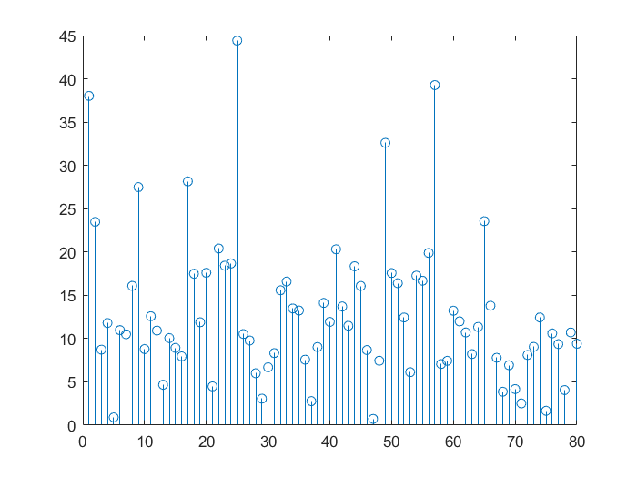
Figure 1: FFT of the received signal.

After performing auto-correlation operation on the data points of the received signal and then FFT operation, the result is as shown in Fig. 2 .

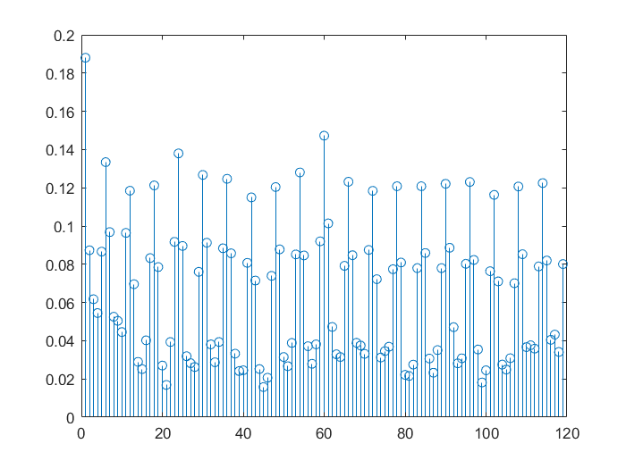
Figure 2: Convolution of frequency domain signal.

In order to further reduce the influence of noise, we divide the data used into multiple segments. These data segments start with the initial point of a single OFDM symbol. The following formula can be obtained by summing each segment of data after auto-correlation operation and then FFT operation.

$$y\left(i,N_{P}\right)=\frac{1}{N_{ch}}\sum_{i_{m}=1}^{N_{ch}}{r\left(N_{P}\cdot\left(i_{m}-1\right)+i\right)}$$ (4)

$$\times{r^{\ast}\left(N_{P}\cdot\left(i_{m}-1\right)+i\right)},$$

$$i=1,2,...,N_{o}\cdot N_{P},$$

$$Y\left(n,N_{P}\right)=\left|\sum_{i=1}^{L_{M}}y(k,N_{P})e^{-jni}\right|,$$ (5)

where $N_{ch}$ is the number of chips, $N_{o}$ is number of chips observed. When $N_{P}$ is the number of points of a single symbol, the peak whose abscissa is an arithmetic progression will appear on $Y\left(n,N_{P}\right)$. At low SNR, the peaks still exist, while the amplitudes of peaks become lower. When $N_{P}$ is not equal to $N_{s}$, peaks that belong to arithmetic progression account for a reduced proportion of all peaks.

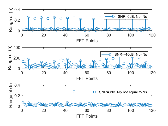
Figure 3: Comparison diagram under different SNR and $N_{P}$.

Then we design a method to find $N_{s}$. According to (4) and (5), the traversal algorithm is proposed: (i) traverse $N_{P}$, (ii) find the abscissa of the peak of $Y\left(n,N_{P}\right)$, (iii) Use algorithm 1 to find out the number of peaks with fixed spacing and the total number of peaks, (iv) use algorithm 2 to find $N_{P}$ which satisfy the judgment conditions and (v) calculate the mean value of all $N_{P}$ that meet the judgment conditions, and judge the calculation result as $N_{s}$. The specific algorithm processes are shown in algorithm I and algorithm 2.

  (A) Initialize: Record the abscissa of all peaks in $Y(n,N_{P})$ (denoted as $k_{\rm{all}}$), the maximum value of $k_{\rm{all}}$ (denoted as $k_{\max}$), amounts of $k_{\rm{all}}$ array $N_{\rm{all}}$, peak spacing $L_{p}=0$, recorded peak $N_{\rm{use}}=0$, temporary peak spacing $L_{\rm{cur}}=0$, the abscissa of current statistics $k_{\rm{cur}}=0$, amount of temporary counted peaks $N_{\rm{cur}}=0$.

  (B) Find the number and spacing of the peaks whose abscissa satisfies the arithmetic sequence:

  for $k_{i}=1;k_{i}<\frac{N_{\rm{all}}}{2};k_{i}=k_{i}+1$ do

     for $k_{j}=k_{i}+1;k_{j}<\frac{N_{\rm{all}}}{2}+2;k_{j}=k_{j}+1$ do

        if $k_{\rm{all}}(k_{j})-k_{\rm{all}}(k_{i})>3$ then

           $N_{\rm{cur}}=2$.

           $L_{\rm{cur}}=k_{\rm{all}}(k_{j})-k_{\rm{all}}(k_{i})$.

           $k_{\rm{cur}}=k_{\rm{all}}(k_{j})$.

           while $k_{\rm{cur}}<k_{\max}$ do

              $k_{\rm{cur}}=k_{\rm{cur}}+L_{\rm{cur}}$.

              if $L_{\rm{cur}}$ is a member of $k_{\rm{all}}$ then

                 $N_{\rm{use}}=N_{\rm{use}}+1$.

                 if $N_{\rm{cur}}>N_{\rm{use}}$ then

                    $N_{\rm{use}}=N_{\rm{cur}}$.

                    $L_{p}=L_{\rm{cur}}$.

                 end if

              end if

           end while

        end if

     end for

  end for

  return  $\left[N_{\rm{use}},N_{\rm{all}},L_{p}\right]$.

Algorithm 1 $\left[N_{\rm{use}},N_{\rm{all}},L_{p}\right]$ = functionA $\left(Y\left(n,N_{P}\right)\right)$

  (A) Initialize: Initialize value $N_{P}$ and its possible minimum and maximum value $N_{\min}$ and $N_{\max}$. Record the array used to store useful $N_{P}$ (Denoted as $P_{u}$). Let $N_{P}=N_{\min}$, $N_{o}=6$.

  (B) Calculate the distance and number between the peaks of $Y(n,N_{P})$ under the current $N_{P}$:

  Generate $Y\left(n,N_{P}\right)$.

  $\left[N_{\rm{use}},N_{\rm{all}},L_{p}\right]$ = functionA $\left(Y\left(n,N_{P}\right)\right)$.

  (C) Determine whether the data is useful:

  if $\frac{N_{\rm{use}}}{N_{\rm{all}}}>0.5$ and $N_{all}>N_{min}$ and $L_{p}=N_{o}$ then

     Store $N_{P}$ in $P_{u}$, $N_{P}=N_{P}+1$.

     if $N_{P}<N_{\max}$ then

        Regenerate $Y\left(n,N_{P}\right)$ .

        $\left[N_{\rm{use}},N_{\rm{all}},L_{p}\right]$ = functionA $\left(Y\left(n,N_{P}\right)\right)$.

        Go to step (C).

     end if

  else

     if There are continuous values in $P_{u}$ tail then

        Remove discontinuous values in $P_{u}$.

        Go to step (D).

     else

        $N_{P}=N_{P}+1$.

        if $N_{P}<N_{\max}$ then

           Regenerate $Y(n,N_{P})$ and $k_{\rm{all}}$.

           $\left[N_{\rm{use}},N_{\rm{all}},L_{p}\right]$ = functionA $\left(Y\left(n,N_{P}\right)\right)$.

           Go to step (C).

        end if

     end if

  end if

  (D) Determine the final value:

  $N_{PL}$ is the length of array $P_{u}$.

  return  $N_{s}=\sum_{k=1}^{N_{PL}}\frac{1}{N_{PL}}P_{u}\left(k\right)$.

Algorithm 2 Traversal method

At last, the improved method achieves 75% accuracy and its Amplitude Error (AE) is between 0.1 and 0.2 under low SNR.

III Calculation of number of carries and useful symbol time by substitution method

For the over-sampled signal, its data points need to be separated before using the above method to estimate $N_{s}$. According to [26], the number of carriers and the oversampling rate are estimated by oversampling the signal and performing a correlation operation, which can be expressed as follows,

$$F_{r}\left(\omega,\tau\right)=\lim_{L_{M}\to\infty}\sum_{i=0}^{L_{M}}\mathbb{E}\left\{r\left(i\right)r^{\ast}\left(i+\tau\right)\right\}\exp\left(-j\tfrac{2\pi}{L_{M}}\omega i\right),$$ (6)

where $L_{M}$ is the amount of using data, $j$ is imaginary part, $r\left(i\right)$ is an over-sampled signal, $F_{r}$ represents power spectral density. Generally, when $\tau=1$, the power spectral density is used in (7). After the above analysis, the estimation formula of oversampling rate is as follows,

$$q=\frac{L_{M}}{L_{p}},$$ (7)

where $L_{p}$ is the distance between the peaks of $F_{r}\left(k,\tau\right)$. After calculating $q$, the signal’s data points are separated to restore the original signal. The symbol length $N_{os}$ of the original signal can be obtained by using the algorithm 1 to process the OFDM received signal without over sampling. The estimation result formula of OFDM carrier number is as follows,

$$N_{cn}=2^{\left(\left\lfloor\log_{2}{\left(N_{os}\right)}\right\rfloor\right)},$$ (8)

where $N_{cn}$ is the OFDM carrier number, $\left\lfloor\cdot\right\rfloor$ represents rounding down to an integer, $q$ is the oversampling rate. After calculating the number of carriers, the length of the OFDM useful symbol can be obtained as follows,

$$N_{u}=q\cdot N_{cn}.$$ (9)

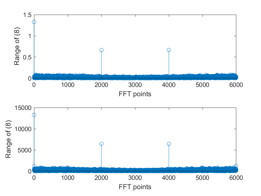
Figure 4: FFT of correlation signal after oversampling when the SNR(dB) is 0 and -40.

The image calculated by (6) is less affected under low SNR. Use $N_{s}$ by algorithm 1 under low SNR can improve the accuracy of the algorithm and reduce the error.

  (A) Initialize:

  Input received signal $r\left(i\right)$.

  (B) Generate $F_{r}$ and calculate $q$:

  $F_{r}\left(k,\tau\right)=\lim_{M\to\infty}\sum_{n=0}^{M}\mathbb{E}\left\{r\left(i\right)\cdot r^{\ast}\left(i+\tau\right)\right\}\cdot$ $\exp\left(-j\tfrac{2\pi}{M}kn\right)$ , $q=\frac{L_{M}}{L_{P}}$.

  (C) Calculate $N_{os}$.

  Under-sample $r\left(i\right)$ and use the result by 1 to calculate $N_{os}$.

  (D) Determine the number of carriers: $N_{cn}=2^{\left(\left\lfloor\log_{2}{\left(N_{os}\right)}\right\rfloor\right)}$.

  (E) Determine $N_{u}$ according to (8):

  return  $N_{u}=q\cdot N_{cn}$.

Algorithm 3 Substitution method

IV Experiment and results

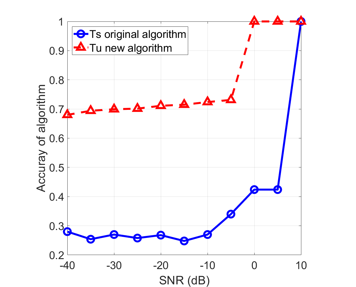
Figure 5: Comparison of symbol length algorithm accuracy.

In this experiment, the modulation mode is 16 Quadrature amplitude modulation (QAM). The number of carriers is 128, the proportion of CP is 0.25. The carrier frequency is 10M. The sampling rate is 40M. The number of symbols is 20. The channel is the Gaussian channel. Set the SNR from -40dB to 10dB. The number of tests under each SNR is $10^{5}$. When SNR is lower than -5dB, we choose 1 to calculate the $N_{s}$. When SNR is higher than -5dB, we choose (3) to calculate the $N_{s}$.

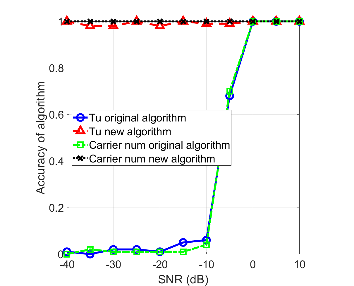
Figure 6: Comparison of useful symbol length and carrier number algorithm accuracy.

By observing the results of the experiments, it can be found that under high SNR, the accuracy of $N_{s}$ and $N_{u}$ are not as good as (2) and (3), and their AEs are about 0.1. The AEs of two algorithms of carrier number have the same performance. At low SNR, the accuracy of the new estimation method for $N_{s}$ and $N_{u}$ is between 0.9 and 1, and the AE is between 0 and 0.15. Compared with the original algorithm, the performance is significantly improved. The accuracy of the carrier number can reach 1 and the AE is 0.

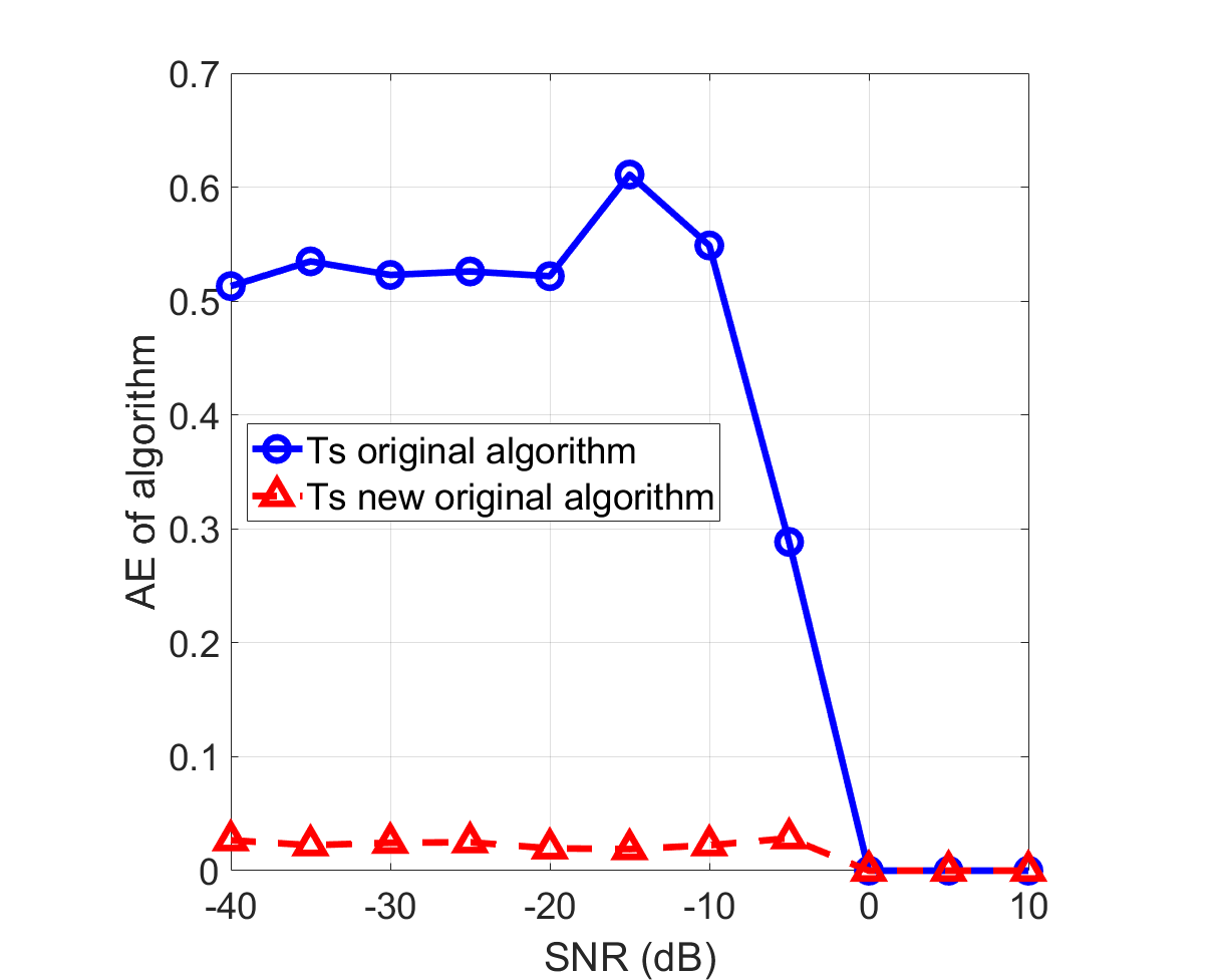
Figure 7: Comparison diagram of symbol length algorithm AE.

The accuracy and AE of $N_{s}$ fluctuate under low SNR. In the experiment, $N_{s}$ is set to 160. Members in $P_{u}$ include $N_{s}$, but their mean value may not be equal to ns. In this case, it is challenging to determine which value is the accurate number of OFDM symbol points. The proposed algorithm improves the AE performance under low SNR.

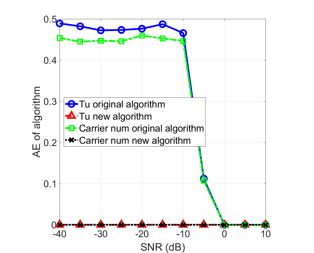
Figure 8: Comparison diagram of symbol length and carrier number algorithm AE.

V Conclusion

This paper proposed an improved algorithm for the total OFDM symbol time $N_{s}$ (reciprocal of symbol rate). Under low SNR, the estimation accuracy has been improved. However, the OFDM useful symbol time that used in the the oversampling rate algorithm is greatly affected by noise. In order to avoid the situation above and improve the performance, the useful symbol time is replaced with the total symbol time. OFDM signal has the characteristic that the number of carriers is exponential of 2. The proposed algorithm can achieve high accuracy. After estimating the number of carriers, the OFDM useful symbol time can be deduced.

References

- [1] X. Zhang, Z. Zheng, W.-Q. Wang, and H. C. So, “DOA estimation of coherent sources using coprime array via atomic norm minimization,” IEEE Signal Processing Letters, vol. 29, pp. 1312–1316, 2022.
- [2] Z. Zhao, Z. Lou, R. Wang, Q. Li, and X. Xu, “I-WKNN: Fast-speed and high-accuracy WIFI positioning for intelligent sports stadiums,” Computers & Electrical Engineering, vol. 98, p. 107619, 2022.
- [3] S. Liu, H. Dahrouj, and M.-S. Alouini, “Joint user association and beamforming in integrated satellite-HAPS-ground networks,” arXiv preprint arXiv:2204.13257, 2022.
- [4] J. Wang, Z. Lu, and Y. Li, “A new CDMA encoding/decoding method for on-chip communication network,” IEEE Transactions on Very Large Scale Integration (VLSI) Systems, vol. 24, no. 4, pp. 1607–1611, 2015.
- [5] J. M. Hamamreh, A. Hajar, and M. Abewa, “Orthogonal frequency division multiplexing with subcarrier power modulation for doubling the spectral efficiency of 6G and beyond networks,” Transactions on Emerging Telecommunications Technologies, vol. 31, no. 4, p. e3921, 2020.
- [6] X. Zhang, Z. Zheng, W.-Q. Wang, and H. C. So, “DOA estimation of mixed circular and noncircular sources using nonuniform linear array,” IEEE Transactions on Aerospace and Electronic Systems, pp. 1–1, 2022.
- [7] A. V. Beliaev and A. O. Kasyanov, “OFDM structural-time parameters estimation,” in Radiation and Scattering of Electromagnetic Waves (RSEMW), Divnomorskoe, Russia, 2019, pp. 324–327.
- [8] Z. Lou, A. Elzanaty, and M.-S. Alouini, “Green tethered UAVs for EMF-aware cellular networks,” IEEE Transactions on Green Communications and Networking, vol. 5, no. 4, pp. 1697–1711, 2021.
- [9] S. Liu, H. Dahrouj, and M.-S. Alouini, “Machine learning-based user scheduling in integrated satellite-HAPs-ground networks,” arXiv preprint arXiv:2205.13958, 2022.
- [10] R. Wang, M. A. Kishk, and M.-S. Alouini, “Ultra-dense LEO satellite-based communication systems: A novel modeling technique,” IEEE Communications Magazine, vol. 60, no. 4, pp. 25–31, 2022.
- [11] D. Ke, Z. Huang, X. Wang, and X. Li, “Blind detection techniques for non-cooperative communication signals based on deep learning,” IEEE Access, vol. 7, pp. 89 218–89 225, 2019.
- [12] E. Azzouz and A. K. Nandi, “Automatic modulation recognition of communication signals,” 2013.
- [13] A. K. Nandi and E. E. Azzouz, “Algorithms for automatic modulation recognition of communication signals,” IEEE Transactions on Communications, vol. 46, no. 4, pp. 431–436, 1998.
- [14] E. E. Azzouz and A. K. Nandi, “Modulation recognition using artificial neural networks,” in Automatic Modulation Recognition of Communication Signals. Springer, 1996, pp. 132–176.
- [15] T. J. O’Shea, J. Corgan, and T. C. Clancy, “Convolutional radio modulation recognition networks,” in International conference on engineering applications of neural networks. Springer, 2016, pp. 213–226.
- [16] Z. Chen, S. Guo, J. Wang, Y. Li, and Z. Lu, “Toward FPGA security in IoT: a new detection technique for hardware Trojans,” IEEE Internet of Things Journal, vol. 6, no. 4, pp. 7061–7068, 2019.
- [17] I. W. Selesnick and M. A. Figueiredo, “Signal restoration with overcomplete wavelet transforms: Comparison of analysis and synthesis priors,” in Wavelets XIII, vol. 7446. International Society for Optics and Photonics, 2009, p. 74460D.
- [18] V. Rajesh and A. A. Rajak, “Channel estimation for image restoration using OFDM with various digital modulation schemes,” in Journal of Physics: Conference Series, vol. 1706, no. 1. IOP Publishing, 2020, p. 012076.
- [19] E. Kanterakis and W. Su, “Blind OFDM parameter estimation techniques in frequency-selective Rayleigh channels,” in IEEE Radio and Wireless Symposium, 2011, pp. 150–153.
- [20] S. Guo, J. Wang, Z. Chen, Y. Li, and Z. Lu, “Securing iot space via hardware trojan detection,” IEEE Internet of Things Journal, vol. 7, no. 11, pp. 11 115–11 122, 2020.
- [21] L. Wang and Y. Li, “Constellation based signal modulation recognition for MQAM,” in 2017 IEEE 9th International Conference on Communication Software and Networks (ICCSN). IEEE, 2017, pp. 826–829.
- [22] P. Liu, B. bing Li, Z. yang Lu, and F. kui Gong, “A blind time-parameters estimation scheme for OFDM in multi-path channel,” in International Conference on Wireless Communications, Networking and Mobile Computing, Wuhan, China, vol. 1, 2005, pp. 242–247.
- [23] J. G. Liu, X. Wang, and J.-Y. Chouinard, “Iterative blind OFDM parameter estimation and synchronization for cognitive radio systems,” in IEEE 75th Vehicular Technology Conference (VTC Spring), Yokohama, Japan, 2012, pp. 1–5.
- [24] T. Yucek and H. Arslan, “OFDM signal identification and transmission parameter estimation for cognitive radio applications,” in IEEE GLOBECOM - Global Telecommunications Conference, Washington, USA, 2007, pp. 4056–4060.
- [25] M. Shi, Y. Bar-Ness, and W. Su, “Blind OFDM systems parameters estimation for software defined radio,” in 2nd IEEE International Symposium on New Frontiers in Dynamic Spectrum Access Networks, Dublin, Ireland, 2007, pp. 119–122.
- [26] M. Dang and G. Sun, “Blind estimation of OFDM parameters under multi-path channel,” in 4th International Congress on Image and Signal Processing, Shanghai, China, vol. 5, 2011, pp. 2809–2812.