Distributed YSOs in the Perseus Molecular Cloud from the Gaia and LAMOST Surveys

Abstract

Identifying the young optically visible population in a star-forming region is essential for fully understanding the star formation event. In this paper, We identify 211 candidate members of the Perseus molecular cloud based on Gaia astronomy. We use LAMOST spectra to confirm that 51 of these candidates are new members, bringing the total census of known members to 856. The newly confirmed members are less extincted than previously known members. Two new stellar aggregates are identified in our updated census. With the updated member list, we obtain a statistically significant distance gradient of $\rm 4.84\;pc\;deg^{-1}$ from west to east. Distances and extinction corrected color-magnitude diagrams indicate that NGC 1333 is significantly younger than IC 348 and the remaining cloud regions. The disk fraction in NGC 1333 is higher than elsewhere, consistent with its youngest age. The star formation scenario in the Perseus molecular cloud is investigated and the bulk motion of the distributed population is consistent with the cloud being swept away by the Per-Tau Shell.

1 Introduction

A complete census of young stellar objects (YSOs) in star-forming regions is important for measuring the statistical properties of young stellar populations and for estimating the star formation rates (e.g., Hsieh & Lai, 2013; Young et al., 2015; Mercimek et al., 2017). Previous studies identified YSOs mainly based on their infrared (IR) excess emission (e.g., Harvey et al., 2007; Evans et al., 2007) or elevated X-ray emission (Stelzer et al., 2012). Various color-color diagrams (CCDs) and color-magnitude diagrams (CMDs) are efficient in selecting sources with IR excess emission. However, these selections are always contaminated by non-YSO sources, such as broad-line active galactic nuclei (AGNs), star-forming galaxies, asymptotic giant branch (AGB) stars, that have similar IR properties as YSOs (Robitaille et al., 2008; Koenig et al., 2012; Manara et al., 2018; Herczeg et al., 2019; Lee et al., 2021). In addition, these CCDs and CMDs are inefficient in selecting evolved YSOs without circumstellar material, which have similar colors as main-sequence stars.

Accurate astrometric measurements from the Gaia mission (Gaia Collaboration et al., 2016) have changed this situation. With measurements of its distance and proper motion of individual sources, membership can be assessed directly, without any assumptions for the source properties. Different methods have been developed to identify new members in nearby star-forming regions, based on Gaia astrometric data, including the following examples. Using the dataset from Gaia DR2 (Gaia Collaboration et al., 2018), Cánovas et al. (2019) identified 166 new candidates in the $\rho$ Ophiuchi region applying different clustering algorithms, including DBSCAN (Ester et al., 1996), HDBSCAN (Campello et al., 2013, 2015; McInnes et al., 2017) and OPTICS (Ankerst et al., 1999). Also in the $\rho$ Ophiuchi region, Grasser et al. (2021) identified additional $\sim$200 new YSO candidates applying the OCSVM algorithm developed by Ratzenböck et al. (2020), based on the dataset from Gaia EDR3 (Gaia Collaboration et al., 2021). Applying a simple thresholding method and utilizing the dataset from Gaia DR2, Luhman (2018) refined the sample of known members and identified new candidates in the Taurus star forming-region, Kubiak et al. (2021) increased the census of known $\epsilon$ Cha members by more than 40%. Both simple thresholding methods and clustering algorithms are powerful tools for identifying new members with high reliability in nearby star-forming regions.

The Perseus molecular cloud is one of the nearest ($\sim$300 pc from the Sun, Ortiz-León et al. (2018)) low mass star-forming regions (Reipurth, 2008). It is a well-studied star-forming region (e.g., Sargent, 1979; Ladd et al., 1993; Kirk et al., 2006; Ridge et al., 2006a; Enoch et al., 2007; Arce et al., 2010) with a range of star-forming environments, both clustered (e.g., the two young clusters NGC 1333 and IC 348) and distributed, as well as several small dense clumps (B1, B5, L1448 and L1455) of the type that often produce one or a few stars (Young et al., 2015). The Perseus molecular cloud has been observed in multi-wavelength studies (e.g., X-ray: Winston et al. 2010; Alexander & Preibisch 2011; Optical: Zhang et al. 2015; IR: Young et al. 2015; sub-millimeter: Kirk et al. 2006; Enoch et al. 2007; radio: Ridge et al. 2006a; Arce et al. 2010). Many YSOs have been identified in this region previously (Evans et al., 2009; Hsieh & Lai, 2013; Young et al., 2015). In a census of members of IC 348 and NGC 1333 using multi-epoch IRAC astrometry, Luhman et al. (2016) identified many members in the two clusters. However, for the remaining cloud regions, only IR excess emission was used to select large samples of YSO candidates (YSOc) (Evans et al., 2009; Hsieh & Lai, 2013; Young et al., 2015), so many undiscovered YSOs without disks may be present in the remaining cloud regions. Recently, Pavlidou et al. (2021) identified five new groups in the Perseus star-forming complex based on the astrometric data from Gaia DR2 (Gaia Collaboration et al., 2018), but they mainly focused on the off-cloud regions specifically, instead of the main cloud regions outside the two young clusters.

In this paper, we use the Gaia astrometry and photometry to identify candidate members in the Perseus molecular cloud, especially in the remaining cloud regions outside the two clusters, and use the LAMOST spectroscopic survey to confirm memberships of these candidates. We describe the datasets used in this work in Section 2, and the source selection procedures in Section 3. The results are presented in Section 4 and discussed in Section 5. We give our summaries and conclusions in Section 6.

2 The Datasets

2.1 Gaia Data

We use the astrometric and photometric data from the Gaia survey (Gaia EDR3) (Gaia Collaboration et al., 2021; Riello et al., 2021; Fabricius et al., 2021) to identify new candidates in the Perseus molecular cloud. We consider only the main cloud region that is covered by the ¹²CO J=1$\to$0 map from the COMPLETE (Coordinated Molecular Probe Line Extinction and Thermal Emission) Survey of Star-Forming Regions (Ridge et al., 2006b), corresponding to $157^{\circ}<l<161.2^{\circ}$ and $-22.2^{\circ}<b<-16.2^{\circ}$. Gaia satellite provides us with very accurate astrometric measurements of almost two billion sources, including $\sim$60,000 within our survey area.

Based on the previously proposed distances to the Perseus molecular cloud, we include only sources with parallaxes between 2.2 and $5.0\ \rm mas$, corresponding to distances of about 200 to $450\ \rm pc$. Only sources whose observations are consistent with the five-parameter model (Lindegren et al., 2018) are retained for further analysis, that is we keep only sources with $ruwe<1.4$ (Gaia Collaboration et al., 2021; Lindegren, 2018). Additional quality cuts are applied to extract sources with high quality astrometry and photometry. Only sources with parallaxes over errors larger than 5 and with proper motion errors less than $0.5\;\rm mas$ are considered to produce astrometrically precise and reliable dataset. Sources with magnitude errors in $G$- or $RP$-bands larger than $0.1\;\rm mag$ are removed to produce high-quality catalog. With these cuts, we extract about 3000 Gaia sources with high quality toward the direction of the Perseus molecular cloud.

2.2 Optical Spectroscopic Data from The LAMOST Survey

We use the spectroscopic data from the data release 7 of the LAMOST survey (LAMOST DR7) (Luo et al., 2022) to confirm memberships of the candidates in the cloud. LAMOST, the Large Sky Area Multi-Object Fiber Spectroscopic Telescope (also called the Guo Shoujing Telescope), is a quasi-meridian Schmidt telescope located at Xinglong Observatory Station in Hebei, China. The telescope has an effective aperture of 3.6$-$4.9 m and a field of view of about $5^{\circ}$ in diameter. The telescope is equipped with 16 spectrographs and 4000 fibers, each spectrograph has a resolution of $\sim$2.5 Å, and the wavelength coverage is 3690$-$9100 Å (Cui et al., 2012; Zhao et al., 2012; Liu et al., 2015).

LAMOST DR7 contains more than 10 million spectra, more than 9.5 million of which are stellar spectra. In the direction of the Perseus molecular cloud, LAMOST obtained more than 9000 spectra of about 5500 distinct sources.

2.3 Additional Ancillary Data

The Perseus molecular cloud has been well covered by many large-sky surveys, including Pan-STARRS1 (Hodapp et al., 2004), 2MASS (Skrutskie et al., 2006), WISE (Wright et al., 2010). The Pan-STARRS1 (PS1) survey images the whole sky in five broadband filters, $grizy$, with a wavelength coverage from 0.4 to $1\;\mu\rm m$ (Stubbs et al., 2010). We retrieve the $griz$ photometry from the PS1 DR1 catalog (Chambers et al., 2016). Sources that are brighter than $14\;\rm mag$ or that have magnitude errors larger than $0.05\;\rm mag$, in $r$ or $i$ filters, are removed to avoid saturation problems and to produce high-quality catalog. The $JHK_{S}$ magnitudes are retrieved from the 2MASS All-Sky Point Source Catalog (Skrutskie et al., 2003) which reaches limiting magnitudes of 15.8, 15.1 and $14.3\ \rm mag$ at 10$\sigma$ for $J$, $H$ and $K_{S}$-bands respectively (Skrutskie et al., 2006). The WISE survey is a mid-infrared full-sky survey undertaken in four bands: $W1$, $W2$, $W3$ and $W4$ bands with wavelengths centered at 3.35, 4.60, 11.56 and $22.09\ \micron$, respectively (Wright et al., 2010). We take the WISE photometry from the AllWISE source catalog (Wright et al., 2019) to determine the presence or absence of circumstellar disks around YSOs.

3 Source Selection

3.1 Census from Previous Studies

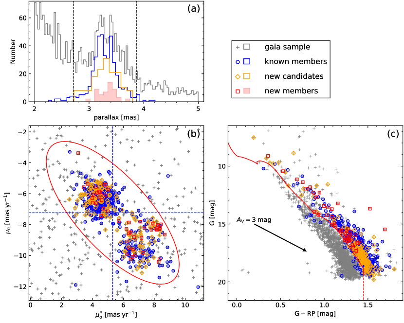
Figure 1: The distributions of parallax (panel a), proper motions (panel b), as well as the $G-RP$ versus $G$ color-magnitude diagram (panel c) for the known members (blue circles and blue histogram), the new candidates (orange diamonds and orange histogram), the new members (red squares and red filled histogram), and the Gaia sample described in Section 2.1 (gray pluses and gray histogram). The vertical dashed lines in panel (a) mark the 3-$\sigma$ interval. The red ellipse in panel (b) is the 3-$\sigma$ confidence ellipse (see the text for detail). The blue vertical and horizontal dashed lines indicate the weighted means of the proper motions along right ascension and declination, respectively. The red solid line in panel (c) is the 10 Myr isochrone from the PARSEC stellar model (Bressan et al., 2012), with solar metallicity and scaled to a distance of 300 pc. The red dashed line corresponding to the color ($G-RP=1.45\;\rm mag$) of the lowest mass star in the PARSEC stellar model. The black arrow is the extinction vector of $A_{V}=3\;\rm mag$ (the typical extinction value of the Perseus sources, see Figure 7) corresponding to the extinction law from Wang & Chen (2019)

Luhman et al. (2016) compiled a thorough census for the two young clusters, and provided samples of 478 and 203 sources with well-confirmed memberships for IC 348 and NGC 1333, respectively. Beginning with this tabulation, we search the literature for additional members in the Perseus molecular cloud, especially in the regions outside the two clusters, with spectroscopically confirmed memberships. We add to our sample the 8 and 2 members identified by Esplin & Luhman (2017) and Luhman & Hapich (2020), respectively. From the Kounkel et al. (2019) search for close companions around young stars, we include in our census the 114 members that have radial velocities between 0 and 25 $\rm km\;s^{-1}$. This velocity range is consistent with the radial velocities of members in IC 348 (Cottaar et al., 2015) and NGC 1333 (Foster et al., 2015). Kounkel et al. (2019) reported radial velocity of $143\ \rm km\;s^{-1}$ for the source 2MASS J03453345+3145553, but Cottaar et al. (2015) reported radial velocity of around $20\ \rm km\;s^{-1}$ from multiple observations, so we retain this object in our member list. Combining all these tabulations together, we arrive at a sample of 805 known members with spectroscopically confirmed memberships in the Perseus molecular cloud.

Cross-matching this list of known members with the Gaia catalog described in Section 2.1, using $2\arcsec$ tolerance, we obtain astrometric and photometric measurements for 406 known members ($\sim$50% of the sample). It is not surprising that about half of the known members are not matched with the Gaia catalog, since that we consider only sources with high-quality Gaia measurements as described in Section 2.1. We would obtain 598 matches, i.e., $\sim$75% of the sample, if no quality cuts were applied to the Gaia catalog. In addition, many of the known members are either too faint ($\sim$150 members in our sample are fainter than $J=16\;\rm mag$, all without matches in the Gaia catalog) or too embedded ($\sim$60 members in the census are deeply embedded class 0/I protostars) to be observed by the Gaia satellite.

Visually inspecting the properties of the 406 matched members, we find that the bulk of these members share common distances, motions and ages, with limited scatter, as expected from their memberships. Figure 1 displays the distributions of parallax and proper motions, as well as the $G-RP$ versus $G$ color-magnitude diagram for these matched known members.

In the parallax distribution in Figure 1, nearly all members have parallaxes within the 3-$\sigma$ interval from the weighted mean parallax. The weighted mean and the weighted standard deviation of the parallax are $\overline{\varpi}=3.29\;\rm mas$ and $\sigma_{\varpi}=0.19\;\rm mas$, respectively, calculated by adopting the inverse of the parallax errors as the weight for each parallax.

In the proper motion distribution in Figure 1, 394 of the matched members have proper motions within the 3-$\sigma$ confidence ellipse (the red ellipse in the plot). The confidence ellipse is calculated as follows. Visually inspecting the distribution of the proper motions, we identify six sources with extreme proper motions (outside the viewing range of the plot). In fact, these outliers are companions around young stars (Kounkel et al., 2019). The weighted means and the weighted standard deviations of the proper motion are $\overline{\mu_{\alpha}^{*}}=5.3\,\rm mas\,yr^{-1}$, $\overline{\mu_{\delta}}=-7.2\,\rm mas\,yr^{-1}$ and $\sigma_{\mu_{\alpha}^{*}}=1.43\,\rm mas\,yr^{-1}$, $\sigma_{\mu_{\delta}}=1.54\,\rm mas\,yr^{-1}$, respectively, calculated by adopting the inverse of the proper motion errors as the weight for each proper motion, excluding the six extreme cases. We also calculate the Pearson correlation coefficient of $-0.7$ between $\mu_{\alpha}^{*}$ and $\mu_{\delta}$ excluding the six extreme cases, considering measurement uncertainties of both axis, by using the Monte Carlo method proposed by Curran (2014). Using the weighted means, the weighted standard deviations and the correlation coefficient, we construct the 3-$\sigma$ confidence ellipse.

From the CMD in Figure 1, we find that all but one members are above or around the 10 Myr isochrone from the PARSEC stellar model (Bressan et al., 2012) with solar metallicity, scaled to a distance of 300 pc. The only source well below the 10 Myr isochrone is 2MASS J03291082+3116427. Considering its location on the CMD and the presence of a disk (Luhman et al., 2016), this object is likely harboring an edge-on disk.

3.2 Candidates and New Members

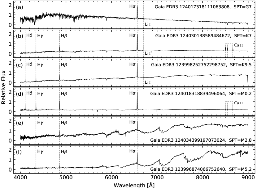
Figure 2: Example spectra of a representative sample of the newly confirmed members. The prominent emission lines and the Li i $\lambda\,6707\,\mathrm{\AA}$ absorption lines are marked in each panel, if present. The Gaia EDR3 source designations and the corresponding spectral types are labeled as well.

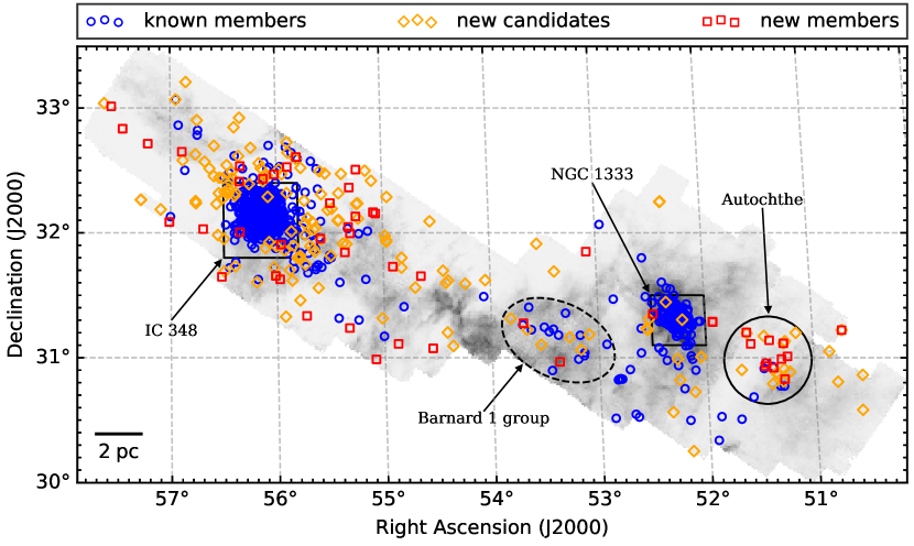
Figure 3: Spatial distribution of previously known members (blue circles), new members (red squares) and candidates (orange diamonds) in the Perseus molecular cloud overlaid on the FCRAO ¹²CO J=1$\to$0 integrated intensity map. The two rectangles mark the sky coverage of the two clusters as defined in Rebull et al. (2007), note that the cluster regions adopted here are slightly different from that in Luhman et al. (2016). The scale bar on the left bottom shows a size of $2\ \rm pc$ at a distance of $300\ \rm pc$. The large solid circle and the dashed ellipse mark the stellar aggregates discussed in Section 5.2.

In the previous section, we find that nearly all the known members have parallaxes within the 3-$\sigma$ of the median parallax for the Perseus members and have proper motions within the 3-$\sigma$ confidence ellipse, as well as that all members are above or around the 10 Myr isochrone. Based on these statistical properties of the known members, we identify new candidates from the Gaia catalog. Specifically, we select a source as a new candidate if it has parallax between 2.71 and 3.87 mas and its proper motion is within the 3-$\sigma$ confidence ellipse defined in the previous section. We also require that the candidate is above the 10 Myr isochrone. As the PARSEC stellar model does not extend down to masses below the hydrogen burning limit, we artificially extend the 10 Myr isochrone vertically to include low mass members. This extension line fits the low mass members fairly well. With these constraints, we select 211 additional candidate members from the Gaia catalog.

Kounkel et al. (2022) studied the Per OB2 association using Gaia EDR3, applying the clustering algorithm HDBSCAN (Campello et al., 2013, 2015; McInnes et al., 2017). In the same region as studied in our work, they discovered 129 new candidate members. In this work, we recover most of these candidates, and identified 109 new YSO candidates. These sources are distributed in the regions with low YSO surface density ($\sim 50\;\mathrm{deg}^{-2}$), and are missed by the HDBSCAN algorithm used in Kounkel et al. (2022).

By cross matching with the LAMOST archive, we obtain optical spectra for 55 candidates. Of these candidates, 38 have broad H$\alpha$ emission lines (characteristic of ongoing accretion activities (Hartmann et al., 1994; Muzerolle et al., 2001)) or Li i $\lambda\,6707\,\mathrm{\AA}$ absorption lines (indicator of youth) in their optical spectra (as shown in Figure 2), indicating that they are bona fide members of the Perseus molecular cloud. Detailed analyses of these emission lines and corresponding accretion activities will be presented in a future paper (Wang, X.-L. et al., in preparation). For the remaining 17 candidates, we did not detect significant emission lines or Li i $\lambda\,6707\,\mathrm{\AA}$ absorption lines in their optical spectra. These 17 candidates include 8 A-type, 4 F-type, 2 G-type, 1 K-type and 2 M-type stars (see Section 4.1 for details of the spectral classification) and most of them show clear H$\alpha$ absorption lines in their optical spectra. Inspecting their locations on the Hertzsprung-Russell (H-R) diagram, we confirm 13 of them as young members. The remaining four objects are classified as main-sequence (MS) stars or asymptotic giant branch (AGB) stars and are rejected from our list of candidates (see Section 5.1 for a discussion).

In summary, we identify 211 candidate members sharing common distances, motions and ages in the Perseus molecular cloud and confirm 51 of them as bona fide members, based on evidences of youth, including the presence of emission lines and Li i $\lambda\,6707\,\mathrm{\AA}$ absorption lines in their optical spectra, and their locations on the H-R diagram. We confirm more than 90% (51/55) of the candidates having LAMOST spectra as Perseus members. These new members and candidates are listed in Table LABEL:tab:new. The spatial distributions of all members (805 known members and 51 new members) and candidates (156 candidates) are displayed in Figure 3. Nearly all the members and candidates newly identified in this work are spread over the whole cloud outside the two young clusters.

4 Stellar Properties

4.1 Spectral Types

In this section, we estimate spectral types for the newly confirmed members, listed in Table LABEL:tab:new. Due to the complexity of classifying YSOs with late spectral types (emission lines and molecular bands), the LAMOST pipeline (Wu et al., 2011; Luo et al., 2015) may give incorrect spectral types during the chi-square fitting procedures. Thus, for objects with automated spectral types from the LAMOST pipeline later than K0, we measured spectral type from the LAMOST spectra by applying the classification scheme from Fang et al. (2017), which focuses on specific spectral features (i.e., VO, TiO and CaH-bands). For sources with earlier types, we adopt the spectral classifications from the LAMOST archive directly. To test the validity of these classification schemes, we apply these classification schemes to a sub-sample of the known members that have been observed by LAMOST as well. The spectral types obtained here and that from the literature are consistent with each other (Figure 4) .

The distributions of spectral types for previously known and newly confirmed members are displayed in Figure 5. Most of the new members are late K and M types. Although we identify many A-, F- and G-type members, the overall distribution of the spectral types remains unchanged. Due to the sensitivity of the LAMOST survey, we did not select any new members later than about M6.

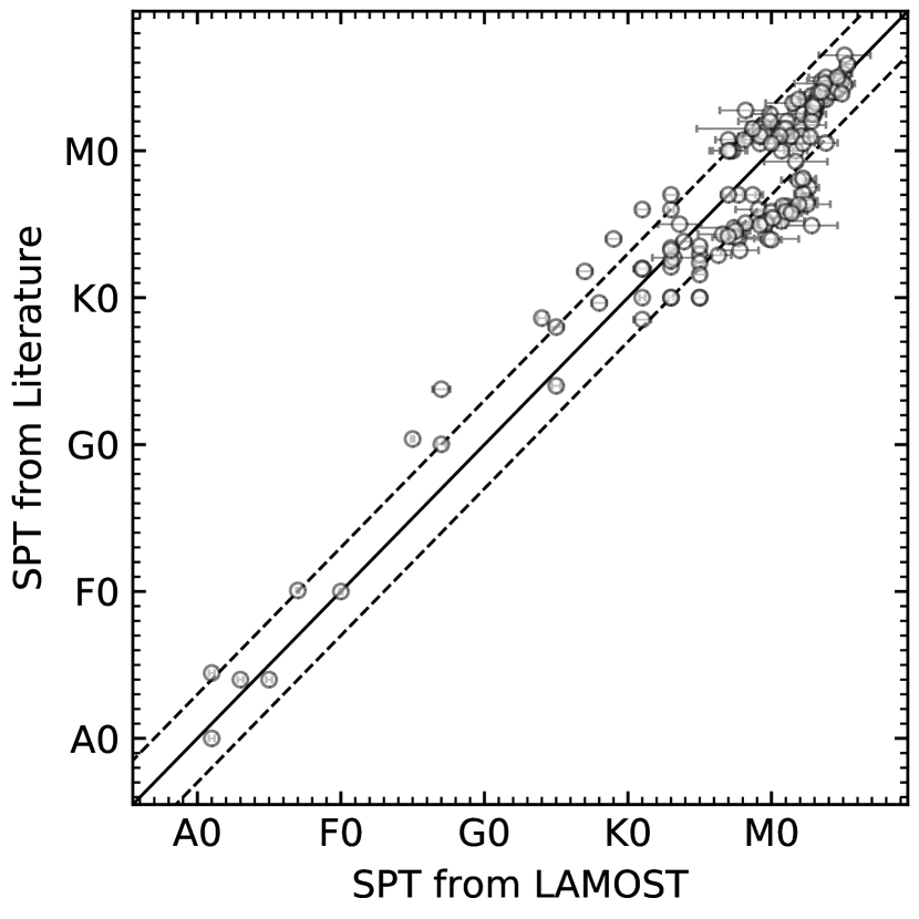
Figure 4: Comparison between spectral types from this work and that from previous works for known members that have LAMOST observations. The solid line indicates the line of equality, and the dashed lines mark differences of 3 sub-types.

4.2 Extinction Corrections

The extinction of each star is determined individually. Intrinsic $g-r$, $r-i$, $i-z$, $z-J$, $J-H$, $H-K_{S}$ colors are estimated with corresponding spectral types for the stars with determined spectral types. For sources later than F0, the relationship from Fang et al. (2017) is adopted, and for earlier type stars that from Covey et al. (2007) is used. These intrinsic colors are converted from the SDSS photometric system to the Pan-STARRS1 photometric system (Tonry et al., 2012), and the extinction values are determined, combining with observed colors and the extinction law from Wang & Chen (2019).

For sources lacking determined spectral types, we can only roughly determine their extinctions with the method described in Fang et al. (2013), in which the extinctions are obtained by employing the $H-K_{S}$ versus $J-H$ color-color diagram. Observed $J-H$ and $H-K_{S}$ colors are compared to intrinsic colors of main-sequence stars (Bessell & Brett, 1988) and T Tauri stars (Meyer et al., 1997), and extinction values are estimated for individual stars, using the extinction law from Wang & Chen (2019) (see Figure 6). The typical error of the extinction values in $V$-band is $\sim$0.6 mag and may be higher for stars with accretion disks.

These extinction values are listed in Table LABEL:tab:new and displayed in Figure 7. The median values of extinction for previously known members, new members and candidates are $A_{V}=3.6$, 2.2 and $2.2\;\rm mag$, respectively. A two sample KS-test also indicates that newly confirmed members and candidates have smaller extinction values than previously known sources. This result is consistent with the fact that most of our newly confirmed members and candidates are spread evenly across the cloud, located at less extincted regions, while most previous searches focused on the two clusters.

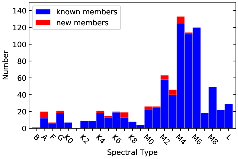
Figure 5: Distributions of spectral types for previously known (blue bars) and newly confirmed (red bars) members.

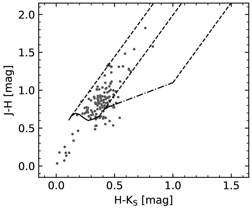
Figure 6: $H-K_{S}$ versus $J-H$ color-color diagram for the candidates in the Perseus molecular cloud. The solid line shows the intrinsic colors for main-sequence stars of K5-M6 types (Bessell & Brett, 1988), and the dash-dotted line is the locus of T Tauri stars from Meyer et al. (1997). The dashed lines are the reddening vectors from Wang & Chen (2019).

5 Discussion

5.1 Membership Confirmations

We assess memberships for about 70% of the candidates having LAMOST spectra as bona fide members based on the existence of H$\alpha$ emission lines or Li i $\lambda\,6707\,\mathrm{\AA}$ absorption lines in their optical spectra in Section 3.2. Similar as in Cieza et al. (2012), we assess memberships for the remaining candidates having LAMOST spectra, but lacking emission lines or Li i $\lambda\,6707\,\mathrm{\AA}$ absorption lines in their optical spectra, according to their locations on the H-R diagram in this section. To construct the H-R diagram, we convert the spectral types to effective temperatures using the empirical relations determined by Fang et al. (2017) for members later than F0-types and by Pecaut & Mamajek (2013) for earlier type members. The observed $J$ magnitudes are dereddened using the extinction values determined in Section 4.2 and distance corrected assuming distances of 300 pc for all sources (see the red filled histogram in panel (a) in Figure 1). The stellar luminosities are then calculated as following.

$$\log\left(\dfrac{L_{\star}}{L_{\odot}}\right)=-\dfrac{BC_{J}+M_{J}-M_{\rm bol,\odot}}{2.5}$$ (1)

where $M_{J}$ is the extinction corrected absolute $J$ magnitude, $BC_{J}$ is the bolometric correction in $J$ band, $M_{\rm bol,\odot}$ is the bolometric magnitude of the Sun. We take $M_{\rm bol,\odot}=4.755\;\rm mag$ (Mamajek, 2012) in this work. The $BC_{J}$ values from Fang et al. (2017) are adopted for spectral types later than F0 and that from Pecaut & Mamajek (2013) for earlier spectral types.

As shown in the H-R diagram (Figure 8), sources having emission lines or Li i $\lambda\,6707\,\mathrm{\AA}$ absorption lines in their optical spectra are all above or around the 10 Myr isochrone, as expected from their memberships. Among the remaining 17 objects lacking emission lines or Li i $\lambda\,6707\,\mathrm{\AA}$ absorption lines in their optical spectra, 13 are located above or around the 10 Myr isochrone and are consistent with being members in the Perseus molecular cloud, 3 are well below the 10 Myr isochrone (marked with open diamonds), and are likely to be field main sequence stars, and one object is well above the stellar birth line (marked with square) and is a possible AGB star.

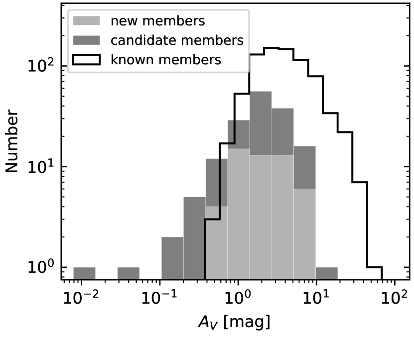
Figure 7: Histograms showing the extinction distributions for previously known members (open histogram), new members (light gray bars) and candidates (dark gray bars).

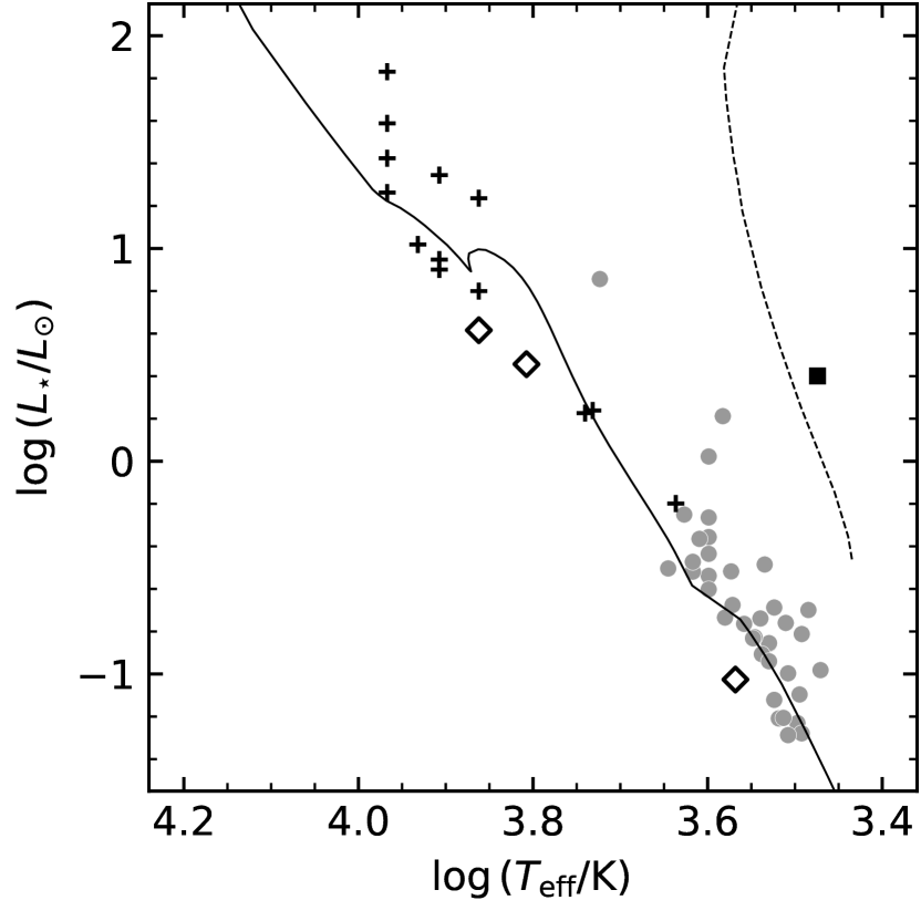
Figure 8: H-R diagram of members identified in this work. Members with and without H$\alpha$ emission lines or Li i $\lambda\,6707\,\mathrm{\AA}$ absorption lines in their optical spectra are marked with gray circles and black pluses, respectively. The solid line is the 10 Myr isochrone and the dashed line is the stellar birth line, from the PARSEC stellar model (Bressan et al., 2012), with solar metallicity. The open diamonds and the square mark stars that are well below the 10 Myr isochrone and that are well above the stellar birth line, respectively.

5.2 Stellar Surface Densities and Substructures in the Perseus Cloud

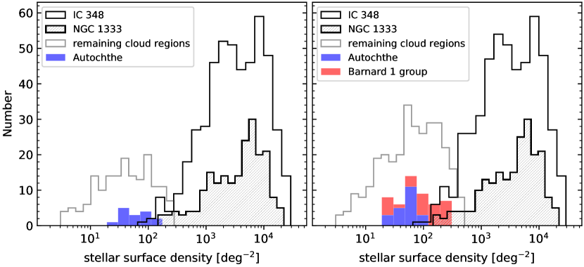
Figure 9: Left: histograms of the stellar surface densities for members in different cloud regions, i.e., IC 348 (black open histogram), NGC 1333 (hatched histogram), the remaining cloud regions (gray open histogram) and Autochthe (blue bars). Right: the same as in the left panel, but for densities including candidate members. The red bars indicate “Barnard 1 group” found in Section 5.2 and marked in Figure 3, stacked on top of that for Autochthe.

YSOs tend to form in clusters and are expected to have higher surface densities than field stars. As mentioned above, there are both clustered and distributed star formation in the Perseus molecular cloud. We have divided the cloud into three regions (i.e., NGC 1333, IC 348 and the remaining cloud regions, following Rebull et al. 2007). We calculate the stellar surface densities $\Sigma$ for individual YSOs as (Casertano & Hut, 1985),

$$\Sigma=\dfrac{n-1}{\pi r_{n}^{2}}$$ (2)

where $n$ is the $n\rm th$ nearest star and $r_{n}$ is the distance to the $n\rm th$ nearest star. We adopt $n=6$ as a surface density reference, the same as that used in Gutermuth et al. (2009).

The resulting stellar surface density distributions are shown in Figure 9 for different cloud regions. The median densities are 3298, 4368 and $42\;\deg^{-2}$ in IC 348, NGC 1333 and the remaining cloud regions, respectively, if only confirmed members (previously known members and newly confirmed members) are included in the density calculations. The stellar surface densities are much higher in the two clusters than in the remaining cloud regions. The star formation environment in the remaining cloud regions is different from that in the clustered regions. The remaining cloud regions represent an environment for distributed star formation. Including the candidate members in the calculation does not change the stellar surface densities in the cluster regions (3236 and $4378\;\deg^{-2}$ for IC 348 and NGC 1333 respectively), but nearly doubles the stellar density in the remaining cloud regions ($69\;\deg^{-2}$).

Visual inspection of Figure 3 shows two additional groupings of YSO(c)s with enhanced stellar densities outside the main clusters IC 348 and NGC 1333. The stellar aggregate toward the western part of the cloud consists of 6 known members, 10 new members and 12 new candidates. This group is associated with the dark cloud L1448 (Lynds, 1962) and was originally identified by Pavlidou et al. (2021), who named the group Autochthe. The stellar aggregate to the east of NGC 1333 consists of 14 known members, 2 new members and 6 new candidates. This group is associated with the dark cloud Barnard 1 (Barnard, 1919) and we designate it as “Barnard 1 group”. These small groups represent the type of star formation that produce a few stars. The stellar densities for Autochthe and the “Barnard 1 group” are included in Figure 9, these density distributions are consistent with the peaks in the distributions for the remaining cloud regions.

We also perform the density-based clustering algorithm DBSCAN (Ester et al., 1996) on our dataset for further examination. When only confirmed members are considered, the algorithm returns 3 clusters, i.e., IC 348, NGC 1333 and Autochthe. The algorithm returned 4 clusters, i.e., IC 348, NGC 1333, Autochthe and “Barnard 1 group”, when the candidates identified in this work are included in the input dataset. These results are consistent with our visual inspection.

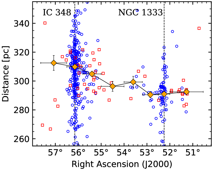
Figure 10: Distance changes along the right ascension direction. The known members and the new members are marked with blue circles and red squares, respectively. The two vertical dashed lines show the locations of the two clusters. The orange filled diamonds with error bars, connected with the solid line show the median distances in individual right ascension bins. The horizontal error bars are the corresponding right ascension ranges, the vertical error bars are the standard deviations of the median values in individual right ascension bins. The standard deviations are calculated from 10000 realizations assuming Gaussian errors (Curran, 2014).

5.3 Distance Gradient

A single distance can not describe the whole cloud accurately, due to the complex structures of the Perseus molecular cloud. Ortiz-León et al. (2018) obtained distances of 321 pc and 293 pc for IC 348 and NGC 1333 respectively, based on VLBA and Gaia measurements.

In this work, we identify about 200 new members and candidates in the Perseus molecular cloud outside the two clusters, and these members spread nearly evenly across the cloud. With these distributed YSOs, as well as the clustered YSOs, we explore potential distance gradient toward the cloud. We measure distances of 310 pc and 291 pc toward IC 348 and NGC 1333, respectively, consistent with that measured by Ortiz-León et al. (2018) within 1-sigma. In Figure 10, we plot the changes of distances along the right ascension direction for all members. We also calculate the median distances of all members in corresponding right ascension bins. As shown in Figure 10, the cloud is getting closer toward us gradually, from east to west. The Spearman’s rank correlation coefficient between right ascension and distance is $|\rho|=0.88$ with $p=0.4\%$, indicating statistically significant correlation between right ascension and distance and that the distance gradient is real. The distance gradient is $4.84\;\rm pc\;deg^{-1}$ from NGC 1333 toward IC 348.

Sargent (1979) found a smoothly varying LSR velocity across the cloud from their CO observations, and Enoch et al. (2006) pointed out that there may also be a distance gradient across the cloud given the velocity gradient. However, we are unable to convert the LSR velocity gradient to a distance gradient directly, since the Perseus molecular cloud is located toward the Galactic anti-center. With our updated member list, we quantify this distance gradient. But it is worth noting that we can not rule out the possibility that the clusters reside in different clouds along the line of sight rather than a single cloud (Bally et al., 2008).

5.4 Evolutionary Stages in Different Cloud Regions

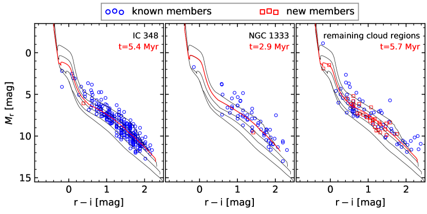
Figure 11: Pan-STARRS1 $r-i$ versus $r$ color-magnitude diagrams for known (blue circles) and new (red squares) members of the Perseus molecular cloud, divided into 3 regions, IC 348 (left), NGC 1333 (middle) and the remaining cloud regions (right). The points have been dereddened and distance corrected. In each panel, the black lines are 1, 3, 10, 30, 100 Myr isochrones, from top to bottom, from the PARSEC stellar model (Bressan et al., 2012), with solar metallicity, and the red solid line is the best fitting isochrone. The resulting ages are labeled.

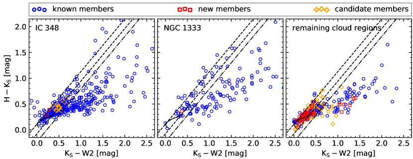
Figure 12: Left panel: infrared color-color plot for members and candidates in IC 348. The blue circles, red squares and orange diamonds mark known members, new members and candidate members, respectively. The black solid line is the locus of dwarfs from Pecaut & Mamajek (2013), the dashed lines correspond to the extinction law from Wang & Chen (2019), enclosing the color space of dwarfs due reddening. The dash-dotted line is 0.15 mag (about 3 times the typical uncertainties in $K_{S}-W2$ colors) redder than the right border of the dwarf locus, serving as the boundary between disk and diskless YSOs. The middle and right panels are the same as the left panel, but for NGC 1333 and the remaining cloud regions, respectively.

In this section, we investigate the evolutionary stages in different cloud regions. Bell et al. (2013) measured an age of $\sim 6\ \rm Myr$ for IC 348, whereas an age of $<1\ \rm Myr$ was measured for NGC 1333 (Wilking et al., 2004). Young et al. (2015) obtained similar conclusion based on the fractions of YSOs at different evolutionary stages. Dividing the Perseus molecular cloud into 3 regions, IC 348, NGC 1333 clusters and the remaining cloud regions (Rebull et al., 2007), we construct the dereddened and distance corrected $r-i$ versus $r$ color-magnitude diagrams for each region (Figure 11). For the cluster regions, we use the median distance for each cluster to do the distance correction, and individual distances are used for individual YSOs in the remaining cloud regions. We fit isochrones from the PARSEC stellar model (Bressan et al., 2012) and estimate ages of 5.4, 2.9 and 5.7 Myr for IC 348, NGC 1333 and the remaining cloud regions, respectively. The age for the remaining cloud regions may be underestimated, since we select only candidates above the 10 Myr isochrone on the $G-RP$ versus $G$ color-magnitude diagram (Panel (c) in Figure 1).

Recently, Kounkel et al. (2022) obtained much younger ages of 2.5 Myr for both IC 348 and NGC 1333, by isochrone fitting of the Gaia photometry to the MIST isochrones (Choi et al., 2016). This discrepancy is mainly due to the difference between the PARSEC stellar model (Bressan et al., 2012) and the MIST isochrones (Choi et al., 2016). We obtain ages of 3.1 and 2.0 Myr for IC 348 and NGC 1333 respectively performing isochrone fitting to the MIST isochrones (Choi et al., 2016). We obtain much older age for IC 348 than for NGC 1333, which is consistent with a higher fraction of diskless objects in IC 348 than in NGC 1333 (Young et al., 2015; Luhman et al., 2016).

We obtain similar age for IC 348 as previous studies (Bell et al., 2013; Luhman et al., 2016). Luhman et al. (2016) proposed an older age for NGC 1333 than previous studies (e.g., Wilking et al., 2004), and they attributed this discrepancy to the distance they assumed for NGC 1333. We obtain much younger age than Luhman et al. (2016), with our updated distance measurements. The remaining cloud regions are significantly older than NGC 1333 and nearly coeval with IC 348. Young et al. (2015) found that the number ratio of PMS stars to protostars in the remaining cloud regions is similar to that in NGC 1333, but significantly smaller than that in IC 348. This discrepancy can be partly explained by the fact that we estimated ages based on optical CMDs, which may bias toward members at later evolutionary stages and thus older ages.

We estimate the fraction of sources harboring disks as another proxy for evolutionary stages of different cloud regions. Luhman et al. (2016) estimated disk fractions of around 40% and 60% for IC 348 and NGC 1333 respectively, with disk fraction defined as $N(\mathrm{II})/N(\mathrm{II+III})$. Based on the source counts reported in Young et al. (2015) (their Table 4), we estimate disk fractions of as high as 82%, 92% and 89% for IC 348, NGC 1333 and the remaining cloud regions, respectively. The discrepancy between the two is mainly due to that Young et al. (2015) used only infrared selected YSOs, whereas Luhman et al. (2016) included many optically visible members, to calculate the disk fractions.

Since many of the new members and candidates identified in this work lack enough Spitzer data to determine its presence or absence of a disk, we use the $K_{S}-W2$ versus $H-K_{S}$ color-color diagram (Figure 12) to determine the presence or absence of a disk. As shown in the plot, sources between the two dashed lines are reddened dwarfs. We consider objects with $K_{S}-W2>0.98\times(H-K_{S})+0.22$ to be those harboring disks. We estimate disk fractions of 45%, 65% and 30%$-$40% for IC 348, NGC 1333 and the remaining cloud regions, respectively, with our updated member list. We estimate similar disk fractions as that estimated by Luhman et al. (2016) for IC 348 and NGC 1333. Including or excluding the new members and candidates in the calculation has little impact on the disk fractions for IC 348 and NGC 1333, since we select few new members and candidates in these regions. But for the remaining cloud regions, we measure a much lower disk fraction compared to that excluding the new members and candidates in the calculation (30%$-$40% compared to 55%). We find that the remaining cloud region is more coeval with IC 348 than with NGC 1333. This result suggests the importance of including Gaia astrometric data in identifying YSOs at more evolved stages, with star-like spectral energy distributions.

5.5 A Possible Scenario for Star Formation in the Perseus Molecular Cloud

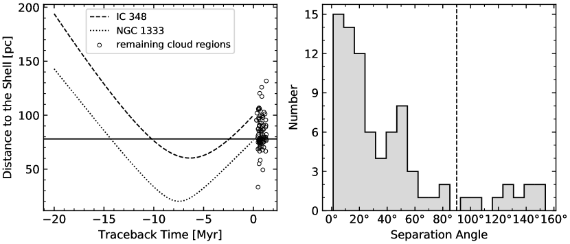
Figure 13: Left panel: distance to the center of the Per-Tau Shell as a function of traceback time. The dashed and dotted lines are stellar traceback lines from Zucker et al. (2022) for IC 348 and NGC 1333 respectively. The horizontal solid line corresponds to a distance of 78 pc, the radius of the shell (Bialy et al., 2021). The circles are individual members in the remaining cloud regions, shifted horizontally with random values to avoid overlap. Right panel: the distribution of separation angles between the velocity vectors and the radial vectors (pointing from the center of the shell to the star) of individual stars. The vertical dashed line indicates separation angle of $90^{\circ}$.

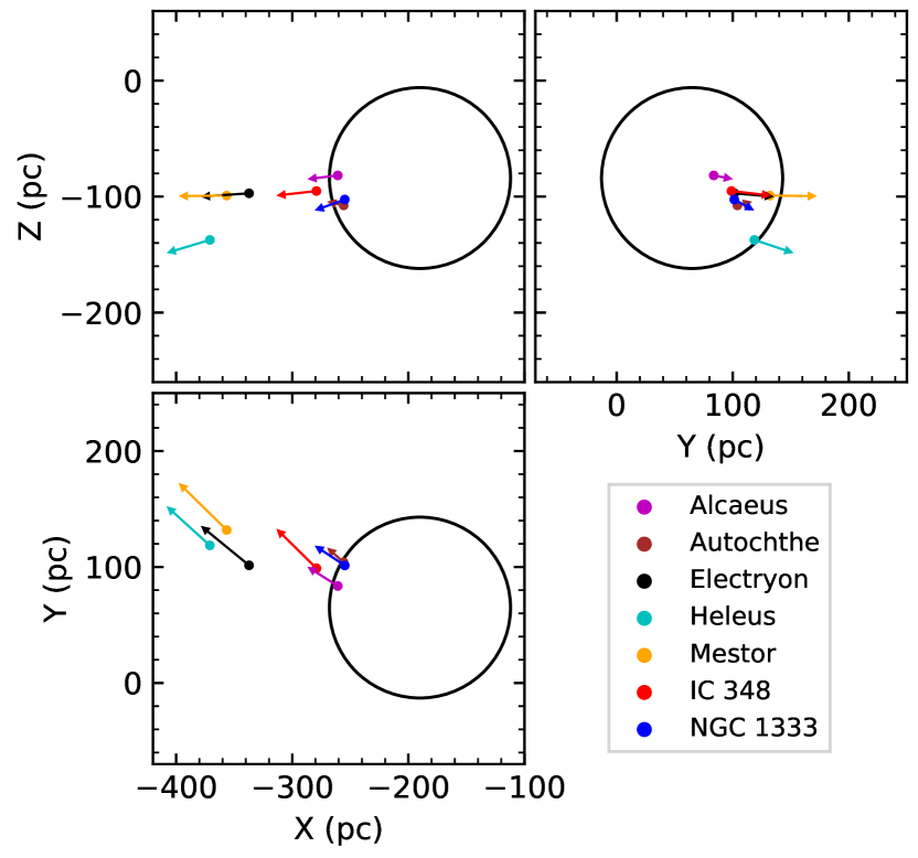
Figure 14: 2D projections of 3D locations of the five groups identified by Pavlidou et al. (2021) in a Heliocentric Galactic Cartesian reference frame. The two famous clusters IC 348 and NGC 1333 are also shown for comparison. Different colors corresponding to different regions as indicated in the legend. The arrows are the velocity vectors of individual groups or clusters. The large circle marks the Per-Tau Shell.

Recently, Zucker et al. (2022) proposed that star formation near the Sun is driven by expansion of the Local Bubble (Cox & Reynolds, 1987) with stellar traceback method. They found that nearly every well-known molecular cloud in the vicinity of the Sun lies on the surface of the Local Bubble, except the Perseus molecular cloud. They attributed this exception to the displacement of the recently discovered Per-Tau Shell (Bialy et al., 2021), containing Perseus on its far side and Taurus on its near side. The stellar traceback data provided by Zucker et al. (2022) indicate that IC 348 and NGC 1333 are moving away from the center of the Per-Tau Shell since about 6$-$8 Myr ago, and that IC 348 has already escaped the shell whereas NGC 1333 is passing through the surface of the shell (as illustrated in the left panel of Figure 13).

Since we double the census of members in the remaining cloud regions, we can investigate the distributed populations with respect to the feedback from the Per-Tau Shell or the Local Bubble. As these distributed populations spread over large areas, it is improper to apply the stellar traceback method to these data, considering the remaining cloud regions as a whole. We investigate motions and locations of individual members relative to the center of the Per-Tau Shell, nearly all of these distributed members have velocities pointing outward the shell with separation angles less than $90^{\circ}$ (as shown in the right panel of Figure 13), about 60% of them have escaped the shell (see the scatter plot in the left panel of Figure 13). These facts may point to the scenario that expansion of the Local Bubble drives the formation of the surface clouds (Zucker et al., 2022) as well as the Perseus molecular cloud, and subsequent expansion of the Per-Tau Shell blows away the Perseus molecular cloud from the Local Bubble’s surface and results in elongated shape of the cloud. This elongation may partly explain the distance gradient confirmed in Section 5.3.

We have searched the literature as well as the Gaia archive for possible massive stars in the vicinity of the cloud that may be responsible for creating the Per-Tau Shell, but no massive stars were found within the region we studied. Bialy et al. (2021) estimated that 2-8 supernova may be responsible for creating such a large shell structure. Since our study is focused on the main cloud region only, detailed analysis of searching for the driving source of the shell is beyond the scope of current study.

Visualizing the five groups identified by Pavlidou et al. (2021) (see Figure 14), we find that the three groups, Electryon, Heleus and Mestor are far away from the Per-Tau Shell, the remaining 2 groups Alcaeus and Autochthe, as well as NGC 1333 and IC 348 are near the surface of the shell. Considering their ages (3-5 Myr, Pavlidou et al. (2021)) and their distances to the shell, the formation of the three off-shell groups are irrelevant to the Per-Tau Shell’s expansion. Alcaeus share similar age as IC 348 and Autochthe is coeval with NGC 1333. These groups may form during the same star formation event.

6 SUMMARY

We have performed a search for new members and candidates in the Perseus molecular cloud, using spectroscopic data from the LAMOST survey and astrometric data from the Gaia survey. The spectral types and extinction corrections are determined for the newly confirmed members. The spatial distributions of the updated member list and the age differences in different cloud regions are investigated. The main contributions are summarized as follows.

1. We have performed a thorough census for new members and candidates in the Perseus molecular cloud and identified 211 candidate members sharing common distances, motions and ages. We identify 51 candidates as new members of the cloud based on evidence of youth including the presence of emission lines or Li i $\lambda\,6707\,\mathrm{\AA}$ absorption lines in their optical spectra and their locations on the H-R diagram, which brings the total number of known members to 856. Due to the sensitivity of the LAMOST survey, we don’t identify any new members later than M6.

2. The stellar aggregate named Autochthe in Pavlidou et al. (2021) is confirmed as a real coeval stellar aggregate with a dozen of confirmed members, with our revised member list. We also identify another small aggregate associated with the dark cloud Barnard 1.

3. The new members are less extincted, and reside in regions with low surface densities. Cloud members in the remaining cloud regions represent the type of distributed star formation, as well as star formation of the type that often produce one or a few stars.

4. A statistically significant distance gradient of $\rm 4.84\;pc\;deg^{-1}$ is measured from west to east. But it is worth noting that the possibility that the two clusters reside in different clouds along the line of sight rather than a single cloud still exists.

5. We estimate similar ages for IC 348 and the remaining cloud regions and NGC 1333 is much younger than the two. The disk fraction in NGC 1333 is higher than in elsewhere, consistent with its youngest age.

6. The bulk motion of the distributed populations is pointed outward of the Per-Tau Shell, and the five groups identified by Pavlidou et al. (2021) are moving away from the shell as well. These are consistent with the star formation scenario proposed by Zucker et al. (2022).

Table 1: Properties of new members and candidates

Gaia EDR3	$\alpha$	$\delta$	$\varpi$	$\mu_{\alpha}^{*}$	$\mu_{\delta}$	SPT	$A_{V}$	membership
	($\deg$)	($\deg$)	(mas)	$\left(\dfrac{\rm mas}{\rm yr}\right)$	$\left(\dfrac{\rm mas}{\rm yr}\right)$		(mag)
120447379950667008	55.085941	30.986461	3.39	6.37	-7.86	$\rm K9.7\pm 1.2$	0.91	member
120460024334304128	54.553027	31.074960	3.35	6.20	-8.28	$\rm M3.7\pm 0.5$	1.04	member
120463116710737920	54.875402	31.110591	3.40	6.69	-8.81	$\rm M4.2\pm 0.5$	0.89	member
120903501181107968	52.162684	30.251784	3.45	7.97	-10.13	$\cdots$	$\cdots$	candidate
120934910278041600	52.333973	30.563745	3.53	7.59	-10.34	$\cdots$	0.42	candidate
120952429448891520	52.122005	30.726234	3.05	4.18	-5.18	$\cdots$	3.45	candidate
120959816792685312	52.255915	30.820725	3.42	7.05	-10.45	$\cdots$	$\cdots$	candidate
120996959670049152	51.678603	30.902172	3.29	7.03	-10.70	$\cdots$	0.38	candidate
121007546764868864	52.051515	31.006618	3.46	5.93	-7.06	$\cdots$	$\cdots$	candidate
121007546764868992	52.050552	31.006813	3.51	6.56	-7.22	$\cdots$	$\cdots$	candidate
121010329903672576	52.272779	30.990384	3.42	6.61	-7.43	$\cdots$	2.90	candidate
121147871936317184	53.372048	30.966361	3.26	7.11	-7.81	$\rm K4\pm 0.4$	4.92	member
121155087481238656	53.540261	31.104290	3.28	7.11	-8.59	$\cdots$	2.33	candidate
121163501321772672	53.170418	31.063100	3.52	7.26	-10.29	$\cdots$	1.22	candidate
121165837783918848	53.273082	31.164778	3.69	8.16	-8.30	$\cdots$	3.22	candidate
121190920393107840	54.362957	31.093630	3.53	6.47	-8.71	$\cdots$	0.69	candidate
121215079583836800	54.412848	31.201997	3.69	5.84	-9.15	$\cdots$	$\cdots$	candidate
121242807893626368	54.416757	31.599503	3.55	7.14	-8.70	$\cdots$	0.26	candidate
121243014052056320	54.395363	31.618091	3.58	6.43	-8.96	$\cdots$	$\cdots$	candidate
121251049934719616	53.667472	31.223274	3.48	7.10	-8.46	$\cdots$	$\cdots$	candidate
121251810145061376	53.700758	31.276131	3.47	7.37	-8.22	$\rm M4.3\pm 0.9$	0.94	member
121252875296947584	53.818389	31.312865	3.64	6.36	-8.68	$\cdots$	0.26	candidate
121284481960254976	54.235610	31.592405	3.30	3.47	-6.04	$\cdots$	2.33	candidate
121286994517121792	54.047228	31.620840	3.34	5.60	-8.36	$\cdots$	$\cdots$	candidate
121291701801318272	54.440752	31.696937	3.23	3.71	-6.09	$\cdots$	2.78	candidate
121352960919189248	53.088591	31.185584	2.98	3.80	-6.58	$\cdots$	1.32	candidate
121389077299717120	52.539279	31.221953	3.54	6.68	-9.74	$\cdots$	$\cdots$	candidate
121394952814977280	52.550734	31.235416	3.43	7.20	-11.12	$\cdots$	$\cdots$	candidate
121396395923984256	52.523196	31.310432	3.40	6.61	-9.56	$\cdots$	0.26	candidate
121399488300436352	52.485424	31.350081	3.49	6.47	-10.23	$\rm M4.1\pm 0.4$	1.26	member
121404573540799232	52.212923	31.304325	3.56	7.68	-9.23	$\cdots$	$\cdots$	candidate
121412849943441024	52.358926	31.445404	3.18	7.52	-9.92	$\cdots$	$\cdots$	candidate
121465046681719552	53.397730	31.690906	3.56	6.87	-8.76	$\cdots$	0.37	candidate
121485903042882304	53.553743	31.912094	3.20	3.34	-6.05	$\cdots$	$\cdots$	candidate
121528504822114176	53.089315	31.849377	3.30	4.86	-5.42	$\rm A3\pm 0.2$	4.94	member
123883147629015424	50.570845	30.582361	2.82	6.73	-7.64	$\cdots$	$\cdots$	candidate
123910081367783552	50.786711	30.807329	3.74	7.63	-7.81	$\cdots$	$\cdots$	candidate
123959834268754176	50.553325	30.862014	3.36	6.80	-7.71	$\cdots$	1.00	candidate
123967049813899008	50.852554	31.051460	3.36	7.91	-7.57	$\cdots$	1.98	candidate
123984027820803456	50.724634	31.221461	2.95	7.95	-7.86	$\cdots$	$\cdots$	candidate
123984027820803584	50.725256	31.220559	2.97	8.68	-8.65	$\rm A1\pm 0.2$	5.81	member
123990517515783680	51.393798	30.791119	3.28	7.84	-8.80	$\cdots$	7.10	candidate
123991277725418752	51.294099	30.809658	3.45	8.03	-9.09	$\cdots$	1.30	candidate
123993373669456000	51.335138	30.865771	3.30	8.35	-8.69	$\cdots$	$\cdots$	candidate
123993506812387712	51.360385	30.877058	3.45	8.37	-8.40	$\cdots$	0.84	candidate
123994679339516800	51.281136	30.828328	3.52	8.14	-8.31	$\rm M2.8\pm 0.3$	1.75	member
123995847570619520	51.229972	30.887357	3.25	7.59	-7.96	$\cdots$	$\cdots$	candidate
123995950649833216	51.281566	30.909474	3.42	8.15	-7.80	$\cdots$	1.00	candidate
123996874066752640	51.379737	30.918846	3.54	8.16	-8.33	$\rm M5.2\pm 0.2$	1.08	member
123998252752298752	51.302425	30.989481	3.41	8.37	-8.21	$\rm K9.5\pm 1.6$	2.21	member
123999730221048320	51.458753	30.931711	3.43	8.33	-8.29	$\rm A1\pm 0.2$	0.97	member
123999936379477504	51.445275	30.955693	3.44	8.24	-8.06	$\rm M4.6\pm 0.6$	2.18	member
124002856957227648	51.582532	31.110303	3.40	8.18	-8.24	$\rm K7\pm 1.6$	4.13	member
124009935063344128	51.245429	31.010398	3.44	8.43	-7.98	$\rm M3.1\pm 0.7$	1.18	member
124016081160908416	51.156870	31.199361	3.12	6.78	-8.66	$\cdots$	3.06	candidate
124017318111063808	51.277991	31.114673	3.40	7.89	-7.92	$\rm G7\pm 0.5$	5.48	member
124017322407087360	51.277117	31.115575	3.31	7.10	-8.20	$\cdots$	$\cdots$	candidate
124017597284939776	51.262843	31.132227	3.40	7.74	-8.18	$\cdots$	2.24	candidate
124018318839496064	51.407963	31.139139	3.33	7.81	-8.33	$\rm M0.2\pm 0.9$	2.54	member
124018864299289088	51.457625	31.173290	3.52	7.98	-8.16	$\cdots$	0.66	candidate
124030138589484672	51.617565	31.202155	3.42	8.21	-8.02	$\rm K7\pm 1.5$	5.81	member
124030138589485440	51.615716	31.194618	3.45	7.95	-8.04	$\cdots$	0.96	candidate
124034399197072896	51.930860	31.288977	3.41	8.34	-10.24	$\rm K4.5\pm 0.6$	1.68	member
124034399197073024	51.926947	31.285487	3.42	8.28	-10.42	$\rm M2.8\pm 0.3$	1.19	member
124475642661236736	52.371350	32.252125	3.60	7.12	-9.40	$\cdots$	$\cdots$	candidate
124475646957597952	52.373574	32.246963	3.62	7.26	-9.43	$\cdots$	0.62	candidate
216418321101566464	56.521716	31.647741	3.18	4.50	-5.91	$\rm M0.3\pm 0.8$	2.35	member
216497829534611072	55.924532	31.327956	2.74	6.25	-7.89	$\cdots$	0.60	candidate
216508790291102464	55.727348	31.334727	3.36	6.36	-8.57	$\rm M3.1\pm 0.3$	1.19	member
216514317913282304	55.787123	31.459427	2.83	5.05	-6.86	$\cdots$	2.44	candidate
216520163364482560	55.972888	31.627645	3.45	6.39	-9.52	$\rm K5\pm 0.3$	0.79	member
216523530618074624	55.857687	31.617337	3.32	4.96	-5.64	$\cdots$	3.47	candidate
216524454036147072	55.880769	31.701164	3.06	4.75	-7.35	$\cdots$	5.97	candidate
216527894305651840	55.328058	31.237570	3.41	6.47	-8.50	$\rm M2.3\pm 0.4$	0.79	member
216543871583951744	55.018656	31.315787	3.42	6.28	-8.42	$\cdots$	$\cdots$	candidate
216563246180936704	55.613452	31.558551	3.80	6.77	-8.96	$\cdots$	$\cdots$	candidate
216572252727848320	55.733078	31.746196	3.12	5.00	-6.93	$\cdots$	4.51	candidate
216572832547750784	55.786991	31.798894	2.82	5.15	-7.54	$\cdots$	2.69	candidate
216572871202364160	55.807903	31.799214	3.20	7.13	-9.74	$\cdots$	$\cdots$	candidate
216575890564466304	55.781245	31.815758	3.46	4.54	-6.29	$\cdots$	0.18	candidate
216585721745264896	55.360264	31.843630	3.13	4.09	-6.06	$\rm K7\pm 0.4$	3.82	member
216587405372443904	55.493524	31.815683	3.34	4.74	-6.96	$\cdots$	$\cdots$	candidate
216587405372444032	55.494163	31.815292	3.30	4.04	-6.54	$\cdots$	$\cdots$	candidate
216588436163846144	55.642520	31.850269	3.00	5.73	-7.57	$\cdots$	3.42	candidate
216588638027403904	55.659161	31.872866	3.18	3.95	-6.01	$\cdots$	5.90	candidate
216588981624788480	55.685585	31.892166	3.53	5.49	-7.06	$\cdots$	7.25	candidate
216590016712558080	55.588347	31.953305	3.39	5.70	-7.76	$\rm M2.5\pm 1.1$	4.30	member
216590016712558208	55.586921	31.946872	3.40	4.84	-8.34	$\cdots$	8.11	candidate
216592039641875712	55.377191	31.914551	3.29	2.51	-6.37	$\cdots$	10.37	candidate
216601213692521472	56.191642	31.604388	3.25	5.13	-6.06	$\cdots$	4.12	candidate
216606268869907072	56.495475	31.690701	2.84	4.63	-5.69	$\cdots$	2.49	candidate
216608948929500032	56.393335	31.732071	3.03	4.24	-5.92	$\cdots$	4.20	candidate
216613999810965760	56.014317	31.655093	3.21	4.02	-6.58	$\rm K7\pm 0.4$	3.37	member
216614034170704256	56.001480	31.656658	3.67	3.54	-7.39	$\cdots$	3.91	candidate
216617641943232128	56.027987	31.722923	3.22	4.33	-5.22	$\cdots$	$\cdots$	candidate
216621004901747584	56.108702	31.877509	3.66	4.97	-6.43	$\cdots$	$\cdots$	candidate
216636505439656960	56.498278	31.951167	2.99	3.23	-6.25	$\cdots$	2.65	candidate
216637982908401792	56.555436	31.982448	2.82	4.55	-5.32	$\cdots$	2.33	candidate
216643480466527744	56.693603	32.030345	3.16	4.73	-5.39	$\rm K7\pm 1.2$	1.71	member
216647603635097856	56.760031	32.237265	3.17	4.37	-5.74	$\cdots$	1.78	candidate
216649218542854400	56.347129	32.004377	3.12	6.60	-10.07	$\rm A5\pm 0.2$	6.14	member
216659457744832512	56.762826	32.254421	3.27	4.31	-5.79	$\cdots$	1.87	candidate
216661519329152000	56.566835	32.231462	3.07	3.88	-5.40	$\cdots$	2.03	candidate
216662687560253696	56.502346	32.279487	3.00	3.90	-5.56	$\cdots$	2.54	candidate
216662790639458816	56.543475	32.317686	3.23	4.58	-6.52	$\cdots$	2.29	candidate
216662992501225984	56.487738	32.328021	3.17	4.13	-6.53	$\cdots$	2.07	candidate
216667150030373376	55.924521	31.858398	3.70	4.38	-5.90	$\cdots$	1.75	candidate
216668013318136320	56.005782	31.893081	2.92	4.67	-6.26	$\cdots$	6.16	candidate
216668803593749888	55.961863	31.905859	3.27	4.86	-6.11	$\rm K3.6\pm 0.7$	2.42	member
216670384140089088	55.841483	31.897773	3.29	4.09	-5.58	$\cdots$	$\cdots$	candidate
216673476518076288	55.862439	32.011624	3.37	5.58	-6.30	$\cdots$	1.97	candidate
216674159417196416	56.072878	31.925330	3.00	4.20	-6.92	$\cdots$	5.81	candidate
216683406482466688	55.732008	31.982894	3.22	3.89	-6.62	$\cdots$	1.43	candidate
216685051453693440	55.732774	32.074545	3.69	4.27	-6.74	$\cdots$	$\cdots$	candidate
216687387916289280	55.651989	32.026197	3.12	4.61	-6.15	$\cdots$	4.46	candidate
216687456635947648	55.632276	32.040875	2.85	4.04	-6.46	$\cdots$	2.45	candidate
216688212549374208	55.663290	32.086597	3.41	4.03	-6.32	$\cdots$	2.60	candidate
216689621299551488	55.707787	32.118134	3.27	4.79	-5.79	$\cdots$	1.89	candidate
216697528334839936	55.736346	32.257784	3.55	3.83	-6.43	$\cdots$	1.10	candidate
216698760989269120	55.901556	32.318429	3.08	4.48	-5.30	$\cdots$	1.80	candidate
216703743151499136	56.393745	32.297036	3.31	3.94	-6.42	$\cdots$	0.14	candidate
216708901408427904	56.256046	32.390130	3.22	4.62	-6.44	$\cdots$	1.00	candidate
216709515586972800	56.454296	32.316288	3.33	4.61	-5.12	$\cdots$	1.90	candidate
216710168422013440	56.450990	32.345797	3.28	3.67	-6.70	$\cdots$	0.04	candidate
216710172718592640	56.447895	32.349759	3.12	3.98	-5.41	$\cdots$	2.65	candidate
216710447596506880	56.383900	32.321349	3.31	3.67	-5.27	$\cdots$	3.61	candidate
216711409669168000	56.432740	32.409746	3.28	4.42	-5.32	$\cdots$	2.29	candidate
216712337382175488	56.588681	32.454909	3.14	3.80	-5.72	$\cdots$	2.15	candidate
216712371741832576	56.537043	32.441361	3.17	4.86	-7.33	$\cdots$	2.70	candidate
216712814121987712	56.502375	32.437318	3.59	4.11	-6.02	$\cdots$	$\cdots$	candidate
216714158448241792	56.347417	32.410264	3.13	4.23	-5.56	$\rm K5.6\pm 1.4$	2.72	member
216714467685880320	56.413167	32.440045	3.11	4.63	-5.62	$\cdots$	$\cdots$	candidate
216714467686233344	56.411139	32.438565	3.30	4.50	-5.50	$\cdots$	$\cdots$	candidate
216716250095746816	56.420118	32.489109	3.69	3.49	-6.71	$\cdots$	2.63	candidate
216716902930786432	56.466634	32.542254	3.14	3.87	-5.82	$\cdots$	1.92	candidate
216718178536050176	56.079724	32.288246	3.07	6.09	-9.73	$\cdots$	$\cdots$	candidate
216721442712788480	56.123493	32.413043	3.20	5.23	-5.52	$\cdots$	2.47	candidate
216721545790356864	56.124912	32.433028	3.16	3.44	-5.58	$\rm A1\pm 0.2$	3.35	member
216721850733091968	56.112591	32.455298	2.77	3.84	-7.37	$\cdots$	$\cdots$	candidate
216723568719908992	56.019145	32.468395	3.39	4.44	-5.86	$\rm M3.3\pm 0.9$	2.17	member
216724088412592640	55.946864	32.468929	3.53	6.76	-9.78	$\cdots$	0.39	candidate
216724668231549056	55.972461	32.509377	3.11	3.68	-6.54	$\cdots$	2.20	candidate
216724775605757312	56.085677	32.461030	3.24	5.00	-6.59	$\cdots$	2.17	candidate
216725424145894400	56.142269	32.517465	2.97	4.23	-6.49	$\cdots$	1.80	candidate
216729139294155520	56.340596	32.535158	3.37	4.24	-6.63	$\rm M3.6\pm 0.3$	2.56	member
216729963927870848	56.355483	32.614519	3.48	4.27	-5.83	$\cdots$	3.56	candidate
216731437100020096	56.161879	32.557035	3.13	4.04	-5.75	$\cdots$	1.65	candidate
216734014080566400	56.238484	32.681098	2.79	3.25	-6.06	$\cdots$	2.65	candidate
216829401012198912	57.012845	32.086724	3.49	6.24	-9.91	$\rm K7\pm 1.1$	0.40	member
216831806193877504	57.093931	32.187523	3.58	6.63	-9.71	$\cdots$	0.81	candidate
216837643052641024	57.280912	32.264721	3.56	6.88	-10.88	$\cdots$	$\cdots$	candidate
216837647349542272	57.280407	32.264269	3.54	6.32	-9.45	$\cdots$	$\cdots$	candidate
217048238186249088	56.882662	32.580982	3.79	7.04	-9.38	$\cdots$	0.61	candidate
217049784373512448	56.890209	32.649548	3.54	7.28	-9.82	$\rm M4.3\pm 0.3$	0.85	member
217068063754243584	57.453438	32.833972	2.94	3.69	-5.37	$\rm M2.8\pm 0.4$	1.15	member
217072186920843264	57.213927	32.714366	3.75	6.23	-9.09	$\rm M2.2\pm 0.4$	0.79	member
217088198561053440	56.629889	32.515255	3.37	3.57	-6.80	$\cdots$	2.94	candidate
217090088346651136	56.674950	32.569818	3.32	4.30	-5.27	$\cdots$	3.05	candidate
217090565086058624	56.761979	32.628750	2.72	3.67	-5.12	$\cdots$	5.03	candidate
217095414105928192	56.584869	32.696801	3.40	6.02	-10.08	$\cdots$	0.55	candidate
217104519434291200	56.746359	32.902363	3.59	4.44	-6.12	$\cdots$	1.72	candidate
217112108642285184	56.396071	32.845285	3.43	2.94	-7.37	$\cdots$	2.58	candidate
217130632837699584	56.947851	33.068172	3.67	4.68	-7.31	$\cdots$	$\cdots$	candidate
217144582891467776	56.850219	33.207827	3.75	6.14	-9.73	$\cdots$	$\cdots$	candidate
217164305382538240	57.561016	33.012804	3.71	6.75	-9.97	$\rm M3.7\pm 0.2$	0.51	member
217165679772064384	57.629022	33.038139	3.49	2.89	-6.91	$\cdots$	0.90	candidate
217304493112912256	54.705249	31.561875	3.18	3.93	-6.33	$\cdots$	3.85	candidate
217307413689579392	54.830994	31.721273	3.53	5.27	-6.90	$\cdots$	5.61	candidate
217313117407234944	54.911635	31.729285	3.28	4.60	-6.41	$\rm A5\pm 0.2$	5.30	member
217317549813446656	54.650193	31.653468	3.49	7.18	-8.87	$\rm M1.8\pm 0.6$	0.50	member
217325555632522624	54.829302	31.800202	3.22	3.03	-6.44	$\cdots$	$\cdots$	candidate
217325555632522880	54.827343	31.800138	3.21	3.67	-7.13	$\cdots$	1.74	candidate
217328300115954560	54.967428	31.929547	3.27	5.10	-6.78	$\cdots$	$\cdots$	candidate
217328300116022528	54.967374	31.940529	2.93	5.53	-6.11	$\cdots$	5.54	candidate
217336825626699008	55.342300	31.909405	3.28	3.83	-6.47	$\cdots$	$\cdots$	candidate
217344041171754368	55.308866	31.996147	3.31	4.58	-6.08	$\rm A5\pm 0.1$	2.78	member
217346167179746176	55.423818	32.098545	3.11	4.28	-5.72	$\cdots$	0.01	candidate
217346377633950464	55.412859	32.102204	3.19	4.52	-5.46	$\cdots$	$\cdots$	candidate
217347232331662976	55.324826	32.047493	3.32	3.99	-6.28	$\rm M3.5\pm 0.4$	2.04	member
217348645376882816	55.229784	32.113858	3.16	4.50	-6.51	$\cdots$	1.49	candidate
217349057693547008	55.253920	32.131725	3.27	4.42	-6.26	$\rm F0\pm 0.1$	6.85	member
217352592451052800	54.981498	31.976198	3.68	5.05	-5.63	$\cdots$	4.35	candidate
217358644060557696	55.065930	32.154617	3.21	4.71	-6.97	$\rm A1\pm 0.2$	2.75	member
217358747139771264	55.087071	32.165668	3.11	5.01	-7.14	$\rm M1.7\pm 0.6$	2.10	member
217363553207422592	55.244151	32.230972	2.92	5.13	-6.11	$\cdots$	1.74	candidate
217363557503130240	55.231857	32.235148	3.20	4.27	-5.80	$\cdots$	2.11	candidate
217383550574612864	54.554583	32.091862	3.56	4.89	-7.50	$\cdots$	$\cdots$	candidate
217407469248673152	54.955579	32.287333	3.13	4.90	-7.10	$\cdots$	1.86	candidate
217415715585859328	55.099042	32.416592	3.10	3.91	-5.66	$\cdots$	$\cdots$	candidate
217440725180229376	55.515644	32.182854	3.31	4.18	-6.31	$\cdots$	5.33	candidate
217440896978922112	55.475918	32.192990	3.28	4.69	-7.20	$\cdots$	3.38	candidate
217444440327486848	55.492348	32.238318	3.22	4.57	-7.43	$\rm G6\pm 0.4$	2.79	member
217446188378685824	55.574839	32.309479	2.88	4.04	-6.44	$\cdots$	1.02	candidate
217455469803469056	55.765457	32.519854	2.84	4.61	-6.53	$\cdots$	$\cdots$	candidate
217457565747541120	55.411412	32.317215	3.32	4.17	-6.25	$\cdots$	1.76	candidate
217458493460476928	55.310242	32.362894	3.18	4.31	-5.93	$\rm M1.1\pm 0.9$	1.99	member
217463643124614656	55.382460	32.472199	3.26	4.53	-6.14	$\cdots$	3.11	candidate
217465876507610112	55.536150	32.474356	3.33	4.21	-5.72	$\cdots$	2.86	candidate
217466361840541952	55.587579	32.494643	3.10	4.14	-6.36	$\cdots$	1.70	candidate
217475123573808000	55.895627	32.526988	3.22	5.03	-5.74	$\rm G5\pm 0.5$	2.98	member
217479414244568320	55.810629	32.592766	3.43	3.57	-6.02	$\cdots$	2.42	candidate
217479521620315264	55.806566	32.607210	3.11	3.08	-3.37	$\rm F0\pm 0.2$	3.22	member
217481269670674048	55.887565	32.642586	2.89	4.39	-5.82	$\cdots$	3.26	candidate
217482850218656512	55.893907	32.724620	3.32	4.11	-7.29	$\cdots$	1.28	candidate
217510376665297152	55.243254	32.506634	3.43	6.63	-9.60	$\rm K5\pm 0.4$	0.54	member
217510892061374208	55.156662	32.497486	3.40	7.17	-9.08	$\cdots$	$\cdots$	candidate
217863938374329472	56.342371	32.921457	3.25	7.45	-10.73	$\cdots$	0.76	candidate

Table 1: – continued

References

- Alexander & Preibisch (2011) Alexander, F., & Preibisch, T. 2011, in The X-ray Universe 2011, ed. J.-U. Ness & M. Ehle, 184. https://ui.adsabs.harvard.edu/abs/2011xru..conf..184A
- Ankerst et al. (1999) Ankerst, M., Breunig, M. M., Kriegel, H.-P., & Sander, J. 1999, SIGMOD Rec., 28, 49, doi: 10.1145/304181.304187
- Arce et al. (2010) Arce, H. G., Borkin, M. A., Goodman, A. A., Pineda, J. E., & Halle, M. W. 2010, ApJ, 715, 1170, doi: 10.1088/0004-637X/715/2/1170
- Astropy Collaboration et al. (2013) Astropy Collaboration, Robitaille, T. P., Tollerud, E. J., et al. 2013, A&A, 558, A33, doi: 10.1051/0004-6361/201322068
- Astropy Collaboration et al. (2018) Astropy Collaboration, Price-Whelan, A. M., Sipőcz, B. M., et al. 2018, AJ, 156, 123, doi: 10.3847/1538-3881/aabc4f
- Bally et al. (2008) Bally, J., Walawender, J., Johnstone, D., Kirk, H., & Goodman, A. 2008, in Handbook of Star Forming Regions, Volume I, ed. B. Reipurth, Vol. 4, 308. https://ui.adsabs.harvard.edu/abs/2008hsf1.book..308B
- Barnard (1919) Barnard, E. E. 1919, ApJ, 49, 1, doi: 10.1086/142439
- Bell et al. (2013) Bell, C. P. M., Naylor, T., Mayne, N. J., Jeffries, R. D., & Littlefair, S. P. 2013, MNRAS, 434, 806, doi: 10.1093/mnras/stt1075
- Bessell & Brett (1988) Bessell, M. S., & Brett, J. M. 1988, PASP, 100, 1134, doi: 10.1086/132281
- Bialy et al. (2021) Bialy, S., Zucker, C., Goodman, A., et al. 2021, ApJL, 919, L5, doi: 10.3847/2041-8213/ac1f95
- Bressan et al. (2012) Bressan, A., Marigo, P., Girardi, L., et al. 2012, MNRAS, 427, 127, doi: 10.1111/j.1365-2966.2012.21948.x
- Campello et al. (2013) Campello, R. J. G. B., Moulavi, D., & Sander, J. 2013, in Advances in Knowledge Discovery and Data Mining, ed. J. Pei, V. S. Tseng, L. Cao, H. Motoda, & G. Xu (Berlin, Heidelberg: Springer Berlin Heidelberg), 160–172. https://link.springer.com/chapter/10.1007/978-3-642-37456-2_14
- Campello et al. (2015) Campello, R. J. G. B., Moulavi, D., Zimek, A., & Sander, J. 2015, ACM Trans. Knowl. Discov. Data, 10, doi: 10.1145/2733381
- Cánovas et al. (2019) Cánovas, H., Cantero, C., Cieza, L., et al. 2019, A&A, 626, A80, doi: 10.1051/0004-6361/201935321
- Casertano & Hut (1985) Casertano, S., & Hut, P. 1985, ApJ, 298, 80, doi: 10.1086/163589
- Cernis (1990) Cernis, K. 1990, AP&SS, 166, 315, doi: 10.1007/BF01094902
- Chambers et al. (2016) Chambers, K. C., Magnier, E. A., Metcalfe, N., et al. 2016, arXiv e-prints, arXiv:1612.05560. https://arxiv.org/abs/1612.05560
- Choi et al. (2016) Choi, J., Dotter, A., Conroy, C., et al. 2016, ApJ, 823, 102, doi: 10.3847/0004-637X/823/2/102
- Cieza et al. (2012) Cieza, L. A., Schreiber, M. R., Romero, G. A., et al. 2012, ApJ, 750, 157, doi: 10.1088/0004-637X/750/2/157
- Cottaar et al. (2015) Cottaar, M., Covey, K. R., Foster, J. B., et al. 2015, ApJ, 807, 27, doi: 10.1088/0004-637X/807/1/27
- Covey et al. (2007) Covey, K. R., Ivezić, Ž., Schlegel, D., et al. 2007, AJ, 134, 2398, doi: 10.1086/522052
- Cox & Reynolds (1987) Cox, D. P., & Reynolds, R. J. 1987, ARA&A, 25, 303, doi: 10.1146/annurev.aa.25.090187.001511
- Cui et al. (2012) Cui, X.-Q., Zhao, Y.-H., Chu, Y.-Q., et al. 2012, RAA, 12, 1197, doi: 10.1088/1674-4527/12/9/003
- Curran (2014) Curran, P. A. 2014, arXiv e-prints, arXiv:1411.3816. https://arxiv.org/abs/1411.3816
- Enoch et al. (2007) Enoch, M. L., Glenn, J., Evans, N. J. I., et al. 2007, ApJ, 666, 982, doi: 10.1086/520321
- Enoch et al. (2006) Enoch, M. L., Young, K. E., Glenn, J., et al. 2006, ApJ, 638, 293, doi: 10.1086/498678
- Esplin & Luhman (2017) Esplin, T. L., & Luhman, K. L. 2017, AJ, 154, 134, doi: 10.3847/1538-3881/aa859b
- Ester et al. (1996) Ester, M., Kriegel, H.-P., Sander, J., & Xu, X. 1996, in Proceedings of the Second International Conference on Knowledge Discovery and Data Mining, KDD’96 (AAAI Press), 226–231. https://www.aaai.org/Papers/KDD/1996/KDD96-037.pdf
- Evans et al. (2007) Evans, N. J. I., Harvey, P. M., Dunham, M. M., et al. 2007, Final Delivery of Data from the C2D Legacy Project: IRAC and MIPS (Pasadena, CA: Spitzer Science Center). https://irsa.ipac.caltech.edu/data/SPITZER/C2D/overview.html
- Evans et al. (2009) Evans, N. J. I., Dunham, M. M., Jørgensen, J. K., et al. 2009, ApJS, 181, 321, doi: 10.1088/0067-0049/181/2/321
- Fabricius et al. (2021) Fabricius, C., Luri, X., Arenou, F., et al. 2021, A&A, 649, A5, doi: 10.1051/0004-6361/202039834
- Fang et al. (2013) Fang, M., Kim, J. S., van Boekel, R., et al. 2013, ApJS, 207, 5, doi: 10.1088/0067-0049/207/1/5
- Fang et al. (2017) Fang, M., Kim, J. S., Pascucci, I., et al. 2017, AJ, 153, 188, doi: 10.3847/1538-3881/aa647b
- Foster et al. (2015) Foster, J. B., Cottaar, M., Covey, K. R., et al. 2015, ApJ, 799, 136, doi: 10.1088/0004-637X/799/2/136
- Gaia Collaboration et al. (2016) Gaia Collaboration, Prusti, T., de Bruijne, J. H. J., et al. 2016, A&A, 595, A1, doi: 10.1051/0004-6361/201629272
- Gaia Collaboration et al. (2018) Gaia Collaboration, Brown, A. G. A., Vallenari, A., et al. 2018, A&A, 616, A1, doi: 10.1051/0004-6361/201833051
- Gaia Collaboration et al. (2021) —. 2021, A&A, 649, A1, doi: 10.1051/0004-6361/202039657
- Gillies & Others (2007) Gillies, S., & Others. 2007, Shapely: Manipulation and Analysis of Geometric Objects. https://github.com/shapely/shapely
- Grasser et al. (2021) Grasser, N., Ratzenböck, S., Alves, J., et al. 2021, A&A, 652, A2, doi: 10.1051/0004-6361/202140438
- Gutermuth et al. (2009) Gutermuth, R. A., Megeath, S. T., Myers, P. C., et al. 2009, ApJS, 184, 18, doi: 10.1088/0067-0049/184/1/18
- Harris et al. (2020) Harris, C. R., Millman, K. J., van der Walt, S. J., et al. 2020, Nature, 585, 357, doi: 10.1038/s41586-020-2649-2
- Hartmann et al. (1994) Hartmann, L., Hewett, R., & Calvet, N. 1994, ApJ, 426, 669, doi: 10.1086/174104
- Harvey et al. (2007) Harvey, P., Merín, B., Huard, T. L., et al. 2007, ApJ, 663, 1149, doi: 10.1086/518646
- Herczeg et al. (2019) Herczeg, G. J., Kuhn, M. A., Zhou, X.-Y., et al. 2019, ApJ, 878, 111, doi: 10.3847/1538-4357/ab1d67
- Hirota et al. (2011) Hirota, T., Honma, M., Imai, H., et al. 2011, PASJ, 63, 1, doi: 10.1093/pasj/63.1.1
- Hirota et al. (2008) Hirota, T., Bushimata, T., Choi, Y. K., et al. 2008, PASJ, 60, 37, doi: 10.1093/pasj/60.1.37
- Hodapp et al. (2004) Hodapp, K. W., Kaiser, N., Aussel, H., et al. 2004, Astronomische Nachrichten, 325, 636, doi: 10.1002/asna.200410300
- Hsieh & Lai (2013) Hsieh, T.-H., & Lai, S.-P. 2013, ApJS, 205, 5, doi: 10.1088/0067-0049/205/1/5
- Hunter (2007) Hunter, J. D. 2007, Computing in Science & Engineering, 9, 90, doi: 10.1109/MCSE.2007.55
- Kirk et al. (2006) Kirk, H., Johnstone, D., & Di Francesco, J. 2006, ApJ, 646, 1009, doi: 10.1086/503193
- Koenig et al. (2012) Koenig, X. P., Leisawitz, D. T., Benford, D. J., et al. 2012, ApJ, 744, 130, doi: 10.1088/0004-637X/744/2/130
- Kounkel et al. (2022) Kounkel, M., Deng, T.-Y., & Stassun, K. G. 2022, arXiv e-prints, arXiv:2206.04703. https://arxiv.org/abs/2206.04703
- Kounkel et al. (2019) Kounkel, M., Covey, K., Moe, M., et al. 2019, AJ, 157, 196, doi: 10.3847/1538-3881/ab13b1
- Kubiak et al. (2021) Kubiak, K., Mužić, K., Sousa, I., et al. 2021, A&A, 650, A48, doi: 10.1051/0004-6361/202039899
- Ladd et al. (1993) Ladd, E. F., Lada, E. A., & Myers, P. C. 1993, ApJ, 410, 168, doi: 10.1086/172735
- Lee et al. (2021) Lee, J.-E., Lee, S., Lee, S., et al. 2021, ApJL, 916, L20, doi: 10.3847/2041-8213/ac0d59
- Lindegren (2018) Lindegren, L. 2018, Re-normalising the Astrometric Chi-square in Gaia DR2, Tech. Rep. GAIA-C3-TN-LU-LL-124-01. http://www.rssd.esa.int/doc_fetch.php?id=3757412
- Lindegren et al. (2018) Lindegren, L., Hernández, J., Bombrun, A., et al. 2018, A&A, 616, A2, doi: 10.1051/0004-6361/201832727
- Liu et al. (2015) Liu, X.-W., Zhao, G., & Hou, J.-L. 2015, RAA, 15, 1089, doi: 10.1088/1674-4527/15/8/001
- Lombardi et al. (2010) Lombardi, M., Lada, C. J., & Alves, J. 2010, A&A, 512, A67, doi: 10.1051/0004-6361/200912670
- Luhman (2018) Luhman, K. L. 2018, AJ, 156, 271, doi: 10.3847/1538-3881/aae831
- Luhman et al. (2016) Luhman, K. L., Esplin, T. L., & Loutrel, N. P. 2016, ApJ, 827, 52, doi: 10.3847/0004-637X/827/1/52
- Luhman & Hapich (2020) Luhman, K. L., & Hapich, C. J. 2020, AJ, 160, 57, doi: 10.3847/1538-3881/ab96bb
- Luo et al. (2022) Luo, A.-L., Zhao, Y.-H., Zhao, G., & al., E. 2022, VizieR Online Data Catalog, V/156. https://ui.adsabs.harvard.edu/abs/2022yCat.5156....0L
- Luo et al. (2015) Luo, A.-L., Zhao, Y.-H., Zhao, G., et al. 2015, RAA, 15, 1095, doi: 10.1088/1674-4527/15/8/002
- Lynds (1962) Lynds, B. T. 1962, ApJS, 7, 1, doi: 10.1086/190072
- Mamajek (2012) Mamajek, E. E. 2012, ApJL, 754, L20, doi: 10.1088/2041-8205/754/2/L20
- Manara et al. (2018) Manara, C. F., Prusti, T., Comeron, F., et al. 2018, A&A, 615, L1, doi: 10.1051/0004-6361/201833383
- McInnes et al. (2017) McInnes, L., Healy, J., & Astels, S. 2017, The Journal of Open Source Software, 2, 205, doi: 10.21105/joss.00205
- Mercimek et al. (2017) Mercimek, S., Myers, P. C., Lee, K. I., & Sadavoy, S. I. 2017, AJ, 153, 214, doi: 10.3847/1538-3881/aa661f
- Meyer et al. (1997) Meyer, M. R., Calvet, N., & Hillenbrand, L. A. 1997, AJ, 114, 288, doi: 10.1086/118474
- Muzerolle et al. (2001) Muzerolle, J., Calvet, N., & Hartmann, L. 2001, ApJ, 550, 944, doi: 10.1086/319779
- Ortiz-León et al. (2018) Ortiz-León, G. N., Loinard, L., Dzib, S. A., et al. 2018, ApJ, 865, 73, doi: 10.3847/1538-4357/aada49
- Pavlidou et al. (2021) Pavlidou, T., Scholz, A., & Teixeira, P. S. 2021, MNRAS, 503, 3232, doi: 10.1093/mnras/stab352
- Pecaut & Mamajek (2013) Pecaut, M. J., & Mamajek, E. E. 2013, ApJS, 208, 9, doi: 10.1088/0067-0049/208/1/9
- Pedregosa et al. (2011) Pedregosa, F., Varoquaux, G., Gramfort, A., et al. 2011, Journal of Machine Learning Research, 12, 2825. http://jmlr.org/papers/v12/pedregosa11a.html
- Ratzenböck et al. (2020) Ratzenböck, S., Meingast, S., Alves, J., Möller, T., & Bomze, I. 2020, A&A, 639, A64, doi: 10.1051/0004-6361/202037591
- Rebull et al. (2007) Rebull, L. M., Stapelfeldt, K. R., Evans, N. J. I., et al. 2007, ApJS, 171, 447, doi: 10.1086/517607
- Reipurth (2008) Reipurth, B. 2008, Handbook of Star Forming Regions, Volume I: The Northern Sky (San Francisco: ASP Monographs). https://ui.adsabs.harvard.edu/abs/2008hsf1.book.....R
- Ridge et al. (2006a) Ridge, N. A., Schnee, S. L., Goodman, A. A., & Foster, J. B. 2006a, ApJ, 643, 932, doi: 10.1086/502957
- Ridge et al. (2006b) Ridge, N. A., Di Francesco, J., Kirk, H., et al. 2006b, AJ, 131, 2921, doi: 10.1086/503704
- Riello et al. (2021) Riello, M., De Angeli, F., Evans, D. W., et al. 2021, A&A, 649, A3, doi: 10.1051/0004-6361/202039587
- Robin et al. (2003) Robin, A. C., Reylé, C., Derrière, S., & Picaud, S. 2003, A&A, 409, 523, doi: 10.1051/0004-6361:20031117
- Robitaille & Bressert (2012) Robitaille, T., & Bressert, E. 2012, APLpy: Astronomical Plotting Library in Python. https://ui.adsabs.harvard.edu/abs/2012ascl.soft08017R
- Robitaille et al. (2008) Robitaille, T. P., Meade, M. R., Babler, B. L., et al. 2008, AJ, 136, 2413, doi: 10.1088/0004-6256/136/6/2413
- Sargent (1979) Sargent, A. I. 1979, ApJ, 233, 163, doi: 10.1086/157378
- Skrutskie et al. (2003) Skrutskie, M. F., Cutri, R. M., Stiening, R., et al. 2003, 2MASS All-Sky Point Source Catalog, IPAC, doi: 10.26131/IRSA2
- Skrutskie et al. (2006) —. 2006, AJ, 131, 1163, doi: 10.1086/498708
- Stelzer et al. (2012) Stelzer, B., Preibisch, T., Alexander, F., et al. 2012, A&A, 537, A135, doi: 10.1051/0004-6361/201118118
- Stubbs et al. (2010) Stubbs, C. W., Doherty, P., Cramer, C., et al. 2010, ApJS, 191, 376, doi: 10.1088/0067-0049/191/2/376
- Tonry et al. (2012) Tonry, J. L., Stubbs, C. W., Lykke, K. R., et al. 2012, ApJ, 750, 99, doi: 10.1088/0004-637X/750/2/99
- Virtanen et al. (2020) Virtanen, P., Gommers, R., Oliphant, T. E., et al. 2020, Nature Methods, 17, 261, doi: 10.1038/s41592-019-0686-2
- Wang & Chen (2019) Wang, S., & Chen, X. 2019, ApJ, 877, 116, doi: 10.3847/1538-4357/ab1c61
- Wilking et al. (2004) Wilking, B. A., Meyer, M. R., Greene, T. P., Mikhail, A., & Carlson, G. 2004, AJ, 127, 1131, doi: 10.1086/381482
- Winston et al. (2010) Winston, E., Megeath, S. T., Wolk, S. J., et al. 2010, AJ, 140, 266, doi: 10.1088/0004-6256/140/1/266
- Wright et al. (2010) Wright, E. L., Eisenhardt, P. R. M., Mainzer, A. K., et al. 2010, AJ, 140, 1868, doi: 10.1088/0004-6256/140/6/1868
- Wright et al. (2019) —. 2019, AllWISE Source Catalog, IPAC, doi: 10.26131/IRSA1
- Wu et al. (2011) Wu, Y., Singh, H. P., Prugniel, P., Gupta, R., & Koleva, M. 2011, A&A, 525, A71, doi: 10.1051/0004-6361/201015014
- Young et al. (2015) Young, K. E., Young, C. H., Lai, S.-P., Dunham, M. M., & Evans, N. J. I. 2015, AJ, 150, 40, doi: 10.1088/0004-6256/150/2/40
- Zhang et al. (2015) Zhang, H.-X., Gao, Y., Fang, M., et al. 2015, RAA, 15, 1294, doi: 10.1088/1674-4527/15/8/014
- Zhao et al. (2012) Zhao, G., Zhao, Y.-H., Chu, Y.-Q., Jing, Y.-P., & Deng, L.-C. 2012, RAA, 12, 723, doi: 10.1088/1674-4527/12/7/002
- Zucker et al. (2022) Zucker, C., Goodman, A. A., Alves, J., et al. 2022, Nature, 601, 334, doi: 10.1038/s41586-021-04286-5