PointFix: Learning to Fix Domain Bias for Robust Online Stereo Adaptation

Abstract

Online stereo adaptation tackles the domain shift problem, caused by different environments between synthetic (training) and real (test) datasets, to promptly adapt stereo models in dynamic real-world applications such as autonomous driving. However, previous methods often fail to counteract particular regions related to dynamic objects with more severe environmental changes. To mitigate this issue, we propose to incorporate an auxiliary point-selective network into a meta-learning framework, called PointFix, to provide a robust initialization of stereo models for online stereo adaptation. In a nutshell, our auxiliary network learns to fix local variants intensively by effectively back-propagating local information through the meta-gradient for the robust initialization of the baseline model. This network is model-agnostic, so can be used in any kind of architectures in a plug-and-play manner. We conduct extensive experiments to verify the effectiveness of our method under three adaptation settings such as short-, mid-, and long-term sequences. Experimental results show that the proper initialization of the base stereo model by the auxiliary network enables our learning paradigm to achieve state-of-the-art performance at inference.

1 Introduction

Stereo depth estimation to predict 3D geometry for practical real-world applications such as autonomous driving [2] has been developed by handcrafted methods [13, 11, 45, 15] and deep stereo models based on supervised learning [25, 4, 36, 17] that leverage the excellent representation power of deep neural networks. In general, given that the high performance of deep networks is guaranteed when test and training data are derived from a similar underlying distribution [6, 24, 14, 22, 7], they demand a huge amount of annotated training data to reflect a real-world distribution. Acquiring groundtruth disparity maps, but unfortunately, is laborious and impractical [38]. Especially for autonomous driving, constructing datasets from all possible different conditions (e.g. weather and road conditions) is impossible while it is a very fatal problem [39]. To mitigate the aforementioned issues, an intuitive solution is to finetune the stereo model trained on a large-scale synthetic dataset that is easier to collect groundtruth. However, despite the help of large-scale synthetic datasets, most recent works [37, 28, 48, 46] have pointed out the limitation of fine-tuning that is incapable of collecting sufficient data in advance when running the stereo models in the open world. While domain generalization methods [44, 34] have shown promising results without real images, they require high computations to provide generalized stereo models and often fail to respond to continuously changing environments.

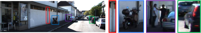
(a) Input image

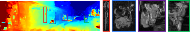
(b) Disparity and reprojection error of MADNet

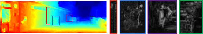
(c) Disparity and reprojection error of PointFix (ours)

Figure 1: Estimated disparity after online adaptation from MADNet and our PointFix. Our method has a much stronger adaptation ability, especially in local detail.

As an alternative solution, online stereo adaptation [39, 38, 41, 31, 47, 21] is proposed to incorporate unsupervised domain adaptation [8, 12] into a continual learning process [33]. Formally, a baseline network is trained offline using a large number of the labeled synthetic datasets (e.g. Synthia [32], FlyingThings3D [25]) and continually adapted to unlabeled unseen scenarios at test time in an unsupervised manner. To demonstrate a faster inference speed for real-world applications, MADNet [39, 31] proposed a lightweight network and modular adaptation framework to rely on self-supervision via reprojection loss [12]. Meanwhile, Learning-to-adapt (L2A) [38] introduced a new learning framework based on model agnostic meta-learning (MAML) [6] for the improved adaptation ability of the network by well-suited base parameters. It shows that the meta-learning framework has great potential in making the network parameters in learning process to make the parameters into a very adaptable state. Despite their great progress, most online adaptation methods [38, 39] have merely attempted to only impose a global average errors from the whole prediction as a learning objective during an offline training without attention to a domain gap in local, showing poor initial performance.

In particular, we observe that given stereo images from a novel environment, incorrectly estimated disparities are concentrated on specific local regions, as depicted in Fig. 5(b). The domain shift [29] issue arises because the local context of test data (e.g. appearance deformations of objects, occlusion type, or the form of a shadow etc.) is significantly diverse from those deployed throughout the training process. This means that without taking such locally varying discrepancies between training and test data into account, the global adaptation strategy used in the existing methods [39, 38, 41, 31, 47, 21] has fundamental limitations in improving the adaptation performance. In addition, a plug-and-play algorithm to easily combine with evolving deep stereo networks is also needed.

In this paper, we propose a novel model-agnostic training method for robust online stereo adaptation, called PointFix, that can be flexibly built on the top of existing stereo models and learns the base stereo network on a meta-learning framework. Unlike the existing methods [31, 21, 5, 41] that focus on a new online adaptation strategy, we leverage the meta-learning strategy for learning-to-fix a base stereo network offline so that it can have generalized initial model parameters and respond to novel environments more robustly. Specifically, we incorporate an auxiliary point-selective network, termed PointFixNet into meta-learning to rectify the local detriment of the base network and alternately fix the base network by an additional update as in the online meta-learning methods [22, 7]. As a result, the parameters of the base network are updated to grasp and utilize the incoming local context and can be robust to the local variants at test time by preventing the network from being biased to global domain dependencies only.

In the experiment, we learn two base stereo models, DispNetC [25], MADNet [39], together with our framework on the synthetic data in the offline training, and then update the whole models (full adaptation) or the sub-module of the models (MAD adaptation) in the online adaptation using the unsupervised reprojection loss [8, 12] on the real-world dataset. Note that the proposed auxiliary network is not used in the online adaptation during inference, maintaining an original inference speed of the base stereo models. Given that our PointFix is a general and synergistic strategy that can be adopted with any kinds of stereo networks, it improves a generalization capability of the base stereo model to novel environments through the robust parameter initialization. Extensive experimental results show that PointFix outperforms recent state-of-the-art results by a significant margin on various adaptation scenarios including short-, mid-, and long-term adaptation. In addition, comparison with domain generalization methods [44, 34, 23] demonstrates the superiority of our PointFix in terms of both accuracy and speed.

2 Related Work

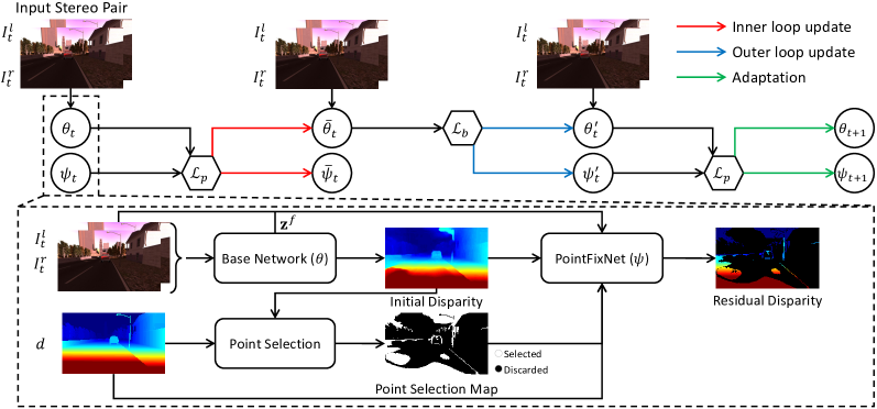
Figure 2: The overall framework of the proposed PointFix and PointFixNet. We alternatively update the base network and PointFixNet underlying meta-learning. The detail of main flowchart is illustrated in the dotted box.

For depth estimation from stereo images, there is an extensive literature, but here we briefly introduce related work in the application of convolutional neural networks (CNNs). Modern approaches using CNNs are mostly categorized by matching-based approaches [43, 17, 35] that learn how to match corresponding points, and regression-based methods [16, 4, 25] that learn to directly regress sub-pixel disparities. To further enhance the performance, some works [19, 18, 30] consider exploiting auxiliary network or module to assist base network by estimating confidence of prediction map from stereo inputs, prediction or cost volume of the base network. Although their results are promising, they have a limitation in retaining the superb accuracy in new domains [31].

Pointing out the domain shift issue, recent works [38, 39, 31, 47, 41, 5, 21] have proposed online stereo adaptation methods to consider more practical solution for real-world applications. They have argued that we should consider a new open-world scenario in which input frames are sequentially provided to the model with certain time intervals. By continually updating parameters at test time in an unsupervised manner, they observe the adaptability of the models in changing environments. As one of the pioneering works, [39, 31] has proposed a light weight model (MADNet) and its modular updating frameworks (MAD, MAD++) to improve the adaptation speed drastically. Following this idea, [41] has picked up the speed even more by implementing ‘Adapt or Hold’ mechanism based on deep Q-learning network [27].

Closely related work to ours is meta-learning based online adaptation approaches [38, 47] that train to learn proper model parameters to be better suitable for online adaptation. L2A [38] has directly incorporated online adaptation process into the inner loop updating process, and also learn a confidence measure to use adaptive weighted loss. However, L2A is inherently unstable during training due to multiple adaptation steps, especially when coupled with the lightweight model (e.g. MADNet [31]). Also, it is worth noting a difference in purpose between confidence-weighted adaptation of L2A and our PointFixNet. The role of the auxiliary network in L2A is to eliminate uncertain errors from inherently noisy reprojection loss, whereas ours is to stabilize the generality of the base model by generating a proper point-wise learning objective for particular bad pixels. We hereby deliver the gradient of the point-wise loss to the base stereo model to prevent the model from being learned by minimizing only the global errors and to remedy domain-invariant representations in local regions.

3 Problem Statement and Preliminaries

3.0.1 Online Stereo Adaptation

Here we first formulate online stereo adaptation. Given stereo image pairs from source domain $\mathcal{D}_{s}$ with available ground-truth maps, online stereo adaptation aims to learn a stereo model capable of adapting itself dynamically in a novel unseen domain $\mathcal{D}_{u}$. In the inference, given a set of parameters $\theta$ from the base stereo model trained on $\mathcal{D}_{s}$, the base network parameters are updated in a single iteration step $t$ to adapt the stereo model with respect to continuous input sequence without ground-truth disparity maps:

$$\theta_{t+1}\leftarrow\theta_{t}-\alpha\nabla_{\theta_{t}}\mathcal{L}_{u}(\theta_{t},I^{l}_{t},I^{r}_{t}),$$ (1)

where $\mathcal{L}_{u}$ is an unsupervised loss function, $\alpha$ is the learning rate, $I^{l}_{t}$, and $I^{r}_{t}$ are left and right images of the $t$-th stereo pair from $\mathcal{D}_{u}$. We evaluate the performance of the online adaptation under the short-term (sequence-level), mid-term (environment-level), and long-term (full) settings. Note that following previous approaches [38, 39], we use a reprojection error [12] as the unsupervised learning objective $\mathcal{L}_{u}$.

3.0.2 Model Agnostic Meta-learning

MAML [6] has proposed to learn initial base parameters that are suited to adapt to new domain with only few updates. This is attained by implementing a nested optimization which consists of an inner loop and an outer loop. Specifically, the inner loop updates the base parameters for each sample in batch separately in the standard gradient descent way. The outer loop performs the update of the base parameters using the sum of sample-specific gradients (meta-gradient) which are computed by the parameters updated in the inner loop. Formally, for a set of tasks $\mathcal{T}$, let the meta-training and meta-testing sets be $\mathcal{D}_{\tau}^{\text{train}}$ and $\mathcal{D}_{\tau}^{\text{test}}$ respectively. A set of parameters $\theta^{*}$ can be obtained for a specific task $\tau\in\mathcal{T}$ with a single gradient step in the inner loop:

$$\theta^{*}=\min_{\theta}\sum_{\tau\in\mathcal{T}}{\mathcal{L}(\theta-\alpha\nabla_{\theta}\mathcal{L}(\theta,\mathcal{D}_{\tau}^{\text{train}}),\mathcal{D}_{\tau}^{\text{test}})},$$ (2)

where $\mathcal{L}$ is a objective function for the task and $\alpha$ is the learning rate. They carries out meta-update, including inner and outer updates, during training and then adaptation for the target task after the the whole meta-learning processes are completely over. In this paper, we treat the disparity prediction for each stereo pair as a single task.

Recent works [22, 7] have introduced two stage meta-learning procedure (a.k.a online meta-learning) that implements meta-update and adaptation stages alternatively during training to achieve more efficient gradient path and better performance. Inspired by their alternative updating scheme, we propose a novel learning-to-fix strategy. Our objective is to get base network and PointFixNet parameters that enable the base network to quickly adapt regardless of local variants in unseen domains. The details are described in the following section.

4 PointFix: Learning to Fix

We design a novel meta-learning framework for online stereo adaptation to learn good base model and quickly adapt to novel environments (i.e., unseen domain), especially concentrating on erroneous pixels. As illustrated in Fig. 6, we leverage off-the-shelf deep stereo model as a base network and incorporate an auxiliary network, PointFixNet, to make parameters of the base network robust to the local distortion.

Algorithm 1 Parameter update with PointFix loss

Input: $\mathcal{I}=\{(I^{l}_{n},I^{r}_{n},d_{n})\}_{n=0}^{N-1}$; learning rate $\alpha$; base model parameters $\theta$; PointFix network parameters $\psi$
Output: updated parameters  $\bar{\theta},~{}\bar{\psi}$

1:function PointUpdate($\mathcal{I},\alpha,\theta,\psi$)

2:     $\mathcal{L}_{p}^{\tau}\leftarrow 0$ $\triangleright$ Initialize loss

3:     for $n=0$ to $N-1$ do

4:         $\hat{d},\mathbf{z}^{b}=\mathcal{F}(I^{l}_{n},I^{r}_{n}|\theta)$

5:         $\mathbf{p}(\theta)=\{(i,j)|~{}|(\hat{d}_{ij}-d_{n,ij})|_{1}>3\}$ $\triangleright$ Select points

6:         $\mathbf{z}^{c}=\mathcal{F}(I^{l}_{n},\hat{d},d_{n}|\psi^{c})$

7:         for $(i,j)\in\mathbf{p}(\theta)$ do

8:              $r_{ij}=\mathcal{F}(\mathbf{z}^{b}_{ij},\mathbf{z}^{c}_{ij}|\psi^{p})$ $\triangleright$ Residual disparity

9:              $\mathcal{L}_{p}^{\tau}\leftarrow\mathcal{L}_{p}^{\tau}+\mathcal{L}_{p}(r_{ij}+\hat{d}_{ij},d_{n,ij})$ $\triangleright$ PointFix loss

10:         end for

11:     end for

12:     $\bar{\theta}\leftarrow\theta-\alpha{\nabla_{\theta}\mathcal{L}_{p}^{\tau}}$ $\triangleright$ Update base network

13:     $\bar{\psi}\leftarrow\psi-\alpha{\nabla_{\psi}\mathcal{L}_{p}^{\tau}}$ $\triangleright$ Update PointFixNet

14:     return $\bar{\theta},\bar{\psi}$

15:end function

Algorithm 2 Overall training procedure

Hyperparameters: batch size $N$; max iteration $K$; learning rate of inner and outer loop $\alpha$, $\beta$
Input: pre-trained base model parameters $\theta$; source training dataset $\mathcal{S}$
Output: optimized base model parameters $\theta^{*}$

1:function Training($\theta,\mathcal{S}$)

2:     Initialize $\theta$ and $\psi$.

3:     for  $k=0$ to $K-1$ do

4:         $\mathcal{L}_{k}\leftarrow 0$ $\triangleright$ Initialize loss

5:         $\mathcal{I}_{k}\sim\mathcal{S}$ $\triangleright$ Sample a batch of size $N$

6:         for  $n=0$ to $N-1$ do

7:              $\theta_{n}\leftarrow\theta,\psi_{n}\leftarrow\psi$ $\triangleright$ Copy parameters

8:              $\bar{\theta}_{n},\bar{\psi}_{n},\leftarrow\text{PointUpdate}(\mathcal{I}_{k,n},\alpha,\theta_{n},\psi_{n})$ $\triangleright$ Inner loop update

9:              $\hat{d}_{n},\textbf{z}^{b}_{k,n}=\mathcal{F}(I^{l}_{k,n},I^{r}_{k,n}|\bar{\theta}_{n})$

10:              $\mathcal{L}_{k}\leftarrow\mathcal{L}_{k}+\mathcal{L}_{b}(\hat{d}_{n},d_{k,n})$ $\triangleright$ Base loss

11:         end for

12:         $\theta^{\prime}\leftarrow\theta-\beta{\nabla_{\theta}\mathcal{L}_{k}}$ $\triangleright$ Outer loop update

13:         $\psi^{\prime}\leftarrow\psi-\beta{\nabla_{\psi}\mathcal{L}_{k}}$ $\triangleright$ Outer loop update

14:         $\theta,\psi\leftarrow\text{PointUpdate}(\mathcal{I}_{k},\alpha,\theta^{\prime},\psi^{\prime})$ $\triangleright$ Adaptation

15:     end for

16:     return $\theta^{*}\leftarrow\theta$

17:end function

4.1 Base Stereo Models

Our goal is to train base models offline to be more suitable for the online adaptation by correcting bias to the seen domain. We have employed two stereo networks as a base model: 1) DispNet-Corr1D [25] (shortened as DispNetC) and 2) MADNet [39]. Besides taking the initial disparity $\hat{d}$ estimated from the base model, we extract intermediate features that is useful to exploit the fine-grained information. The intermediate features consist of the matching cost $\mathbf{c}$ (same as correlation layer in DispnetC) and its corresponding left feature $\mathbf{f}^{l}$. They are concatenated and taken as a base feature $\mathbf{z}^{b}=\Pi(\mathbf{c},\mathbf{f}^{l})$, where $\Pi(\cdot,\cdot)$ is a concatenation operation. We note that in MADNet, the matching cost calculation is similar with the one in DispNetC, but before calculation their right features are warped with a disparity map on a coarse resolution to reduce search range and computation. However, to extract base features, we apply the same matching cost computation scheme used in DispNetC regardless of the base network to ensure the generality of our method.

In each inner loop of our method, we select a pixel $i,j$ to fix local deformations by computing $\ell_{1}$ loss between $\hat{d}$ and the ground-truth $d$, such that the set of points $\mathbf{p}(\theta)$ with the base parameter $\theta$ can be derived as:

$$\mathbf{p}(\theta)=\{(i,j)|~{}|\hat{d}_{ij}-d_{ij}|_{1}>3\}.$$ (3)

Note that we represent $\mathbf{p}$ as a function of $\theta$ to indicate that the selected point varies depending on $\theta$ updated in the learning procedure. In next section, we describe a way to leverage the set of points for correcting local distortions caused by the seen domain bias, depicted in Fig. 5.

4.2 PointFixNet

To mitigate the seen domain bias of the base network, we deploy an additional auxiliary network, called PointFixNet, which individually repairs a disparity by incurring a proper point-wise gradient. The PointFixNet consists of two modules: a feature extraction module (parameterized by $\psi^{c}$) that extracts feature $\mathbf{z}^{c}$ from heterogeneous inputs; and a point-wise prediction module (parameterized by $\psi^{p}$) that generates residual disparity value of each point and back-propagates the point-wise errors. Specifically, the feature extraction module consists of three convolution layers and takes the left image, $I^{l}$, the initial disparity $\hat{d}$, and ground-truth $d$ as inputs to integrate context around each erroneous pixel. Therefore, the feature $\mathbf{z}^{c}$ can be obtained as follows:

$$\mathbf{z}^{c}=\mathcal{F}(I^{l},\hat{d},d|\psi^{c}),$$ (4)

where $\mathcal{F}$ is a feed-forward process.

Then, the base feature $\mathbf{z}^{b}$ from the base network and feature $\mathbf{z}^{c}$ from the feature extraction module are concatenated and fed into the point-wise prediction module to generate the residual disparity value $r_{ij}$. Inspired by structure in  [20], the module consists of four fully-connected (FC) layers to produce a single value for each pixel, such that:

$$r_{ij}=\mathcal{F}(\mathbf{z}^{b}_{ij},\mathbf{z}^{c}_{ij}|\psi^{p}),$$ (5)

where $(i.j)\in\mathbf{p}(\theta)$. The final disparity for $(i,j)$-th pixel is obtained by adding $r_{ij}$ to $\hat{d}_{ij}$. We note that FC layers share weights across all selected points.

4.3 Learning to Fix

The key idea underlying our framework is iterating learning how to fix first and then fixing alternatively. First, the parameters of the PointFixNet learn how to generate a proper gradient to the base model in a point-wise manner such that the base model can be improved with less domain bias and then secondly the base model is updated by the learned PointFixNet. This strategy is essential because if we keep network training only with point loss, the performance of prediction after PointFixNet can be guaranteed but the one after the base model may not. Thus, to enhance maximal performance of the base network, it is necessary to employ the alternative meta-learning structure. To this end, we deploy two loss functions: a base loss, $\mathcal{L}_{b}$, derived from the whole disparity map predicted by the base network and a point loss, $\mathcal{L}_{p}$, applied to the final disparity values. They are alternatively optimized to update $\theta$ and $\psi$ by relying on the two-stage meta-learning scheme [22, 7], as described in Fig. 6 and Alg. 2.

In the inner loop, parameters are copied for each sample in batch, $\theta_{n}\leftarrow\theta$ and $\psi_{n}\leftarrow\psi$. Then we calculate the PointFix loss, to evaluate of the current parameters:

$$\bar{\theta}_{n}\leftarrow\theta_{n}-\alpha\nabla_{\theta_{n}}\sum\nolimits_{(i,j)\in\mathbf{p}(\theta)} \mathcal{L}_{p}(\hat{d}_{ij}+r_{ij},d_{ij}),$$ (6)

$$\bar{\psi_{n}}\leftarrow\psi_{n}-\alpha\nabla_{\psi_{n}}\sum\nolimits_{(i,j)\in\mathbf{p}(\theta)} \mathcal{L}_{p}(\hat{d}_{ij}+r_{ij},d_{ij}),$$ (7)

where $\alpha$ is a learning rate, $\mathbf{p}({\theta}$) is a set of selected points, and $\mathcal{L}_{p}$ is a point-wise $\ell_{1}$ loss between the final disparity and its corresponding ground-truth. Given in Alg. 1, since the PointFix loss is imposed on the local distortion of the erroneous pixels selected on the initial prediction, we can update base parameters that refer to the fine-grained details.

In the outer loop, we evaluate the performance of the updated base parameter after the inner loop. To measure the performance, we apply the conventional supervised loss between the initial disparity map and ground-truth. Following the procedure of [6], the parameters $\theta$ and $\psi$ are updated based on sum of $\mathcal{L}_{k}$ as follows:

$$\theta^{\prime}\leftarrow\theta-\beta\nabla_{\theta}\mathcal{L}_{k},~{}~{}~{}\psi^{\prime}\leftarrow\psi-\beta\nabla_{\psi}\mathcal{L}_{k},$$ (8)

where $\mathcal{L}_{k}=\sum_{N}\mathcal{L}_{b}(\hat{d}_{n},d_{k,n})$ and $k$ is the current iteration step. Note that the gradients are computed along with the parameters before being updated in the inner loop.

Unlike traditional MAML where the parameters are optimized via meta-update only, we deploy an additional update inspired by online meta-learning. $\theta^{\prime}$ and $\psi^{\prime}$ are updated in the same way as the inner loop so that the parameters after final update, $\theta$ and $\psi$ can be written as:

$$\theta\leftarrow\theta^{\prime}-\alpha{\nabla_{\theta^{\prime}}\sum\nolimits_{(i,j)\in\mathbf{p}(\theta^{\prime})}\mathcal{L}_{p}(\hat{d}_{ij}+r_{ij},d_{ij})},$$ (9)

$$\psi\leftarrow\psi^{\prime}-\alpha{\nabla_{\psi^{\prime}}\sum\nolimits_{(i,j)\in\mathbf{p}(\theta^{\prime})}\mathcal{L}_{p}(\hat{d}_{ij}+r_{ij},d_{ij})},$$ (10)

where $r_{ij}=\mathcal{F}(\mathbf{z}_{ij}^{b},\mathbf{z}_{ij}^{c},d_{ij}|\bar{\psi}^{p})$ for $(i,j)\in\mathbf{p}(\theta^{\prime})$. Finally, the networks are updated with PointFix loss which are, at the first stage, trained to generate proper back-propagation to enhance the performance of the base network in the next training step. At test time, we use the final parameters of the base network $\theta^{*}$ and perform adaptation according to Eq. (1).

5 Experiments

5.1 Experimental Settings

5.1.1 Datasets.

In order to evaluate our method on realistic scenario, we use synthetic dataset for offline training and real dataset for the test. Therefore, the training and test data exist in completely different data distributions. Following the previous work [38], we train our networks using the Synthia [32] dataset and evaluate each model on the KITTI-raw [9] dataset and the subset of the DrivingStereo [42] dataset. All datasets are recorded in driving scene but the Synthia [32] is synthetic data, the KITTI and DrivingStereo are obtained from real world. The Synthia [32] dataset contains 50 sequences which have different combination of weathers, seasons and locations. To set similar disparity ranges in training and test, we resized Synthia [32] dataset images to half resolution as in [38]. We exploit stereo images from front direction only and there are 45,591 total number of stereo frames. The KITTI [9] dataset consists of 71 sequences and total 42,917 frames of stereo images and sparse depth maps. Different from the scenario on the KITTI [9] dataset, we present an additional adaptation scenario that the models adapt to various unseen weather conditions using the subset of the DrivingStereo [42] dataset. The DrivingStereo contains four different weather sequences (i.e., cloudy, foggy, rainy, and sunny) that each sequence includes 500 stereo images with high quality labels obtained from multi-frame LiDAR points.

5.1.2 Metrics.

We evaluate the performance using two popular evaluation metrics, the percentage of pixels with disparity outliers larger than 3 (D1-all) and average end point error (EPE). Following the scheme of [39, 38], we average each score from all the frames which belong to the same sequence and reset the model to the base parameters at the next sequence, based on the definition of a sequence for different evaluation protocols.

5.1.3 Evaluation protocols.

We perform online stereo adaptation under three different settings according to the definition of the sequence, including short-, mid-, and long-term adaptation. For short-term adaptation, each sequence is defined as a distinct sequence provided by the dataset (e.g. 2011_09_30_drive_0028_sync). This setting is appeared in [38]. The sequences in mid-term adaptation are divided according to the environment (i.e., City, Residential, Campus, Road). In long-term adaptation, we perform adaptation for all frames by concatenating all mid-term sequences. The mid- and long-term adaptation settings are shown in [39] as short- and long-term adaptation. The implementation details are provided in supplementary material.

Table 1: Mid-term adaptation: Performance comparison for several methods on the KITTI [9] dataset.

Method	Training	Adapt.	City		Residential		Campus		Road		Avg.
			D1-all	EPE	D1-all	EPE	D1-all	EPE	D1-all	EPE	D1-all	EPE
DispNetC-GT	KITTI	No	1.94	0.68	2.43	0.77	5.43	1.10	1.67	0.69	2.87	0.81
MADNet-GT	KITTI	No	2.05	0.65	2.67	0.82	6.87	1.24	1.57	0.66	3.29	0.84
L2A-Disp.	Synthia	No	12.78	1.67	12.80	1.72	17.57	2.06	12.34	1.59	13.87	1.76
MADNet	Synthia	No	38.78	8.36	35.73	7.89	40.59	7.68	38.31	8.77	38.35	8.18
Ours-Disp.	Synthia	No	9.98	1.47	10.99	1.62	17.01	2.06	7.98	1.33	11.49	1.62
Ours-MAD.	Synthia	No	15.51	1.82	14.24	1.78	22.40	3.04	15.61	1.84	16.94	2.12
L2A-Disp.	Synthia	Full	2.05	0.78	2.57	0.86	4.43	1.07	1.63	0.77	2.67	0.87
MADNet	Synthia	Full	2.11	0.81	2.79	0.90	6.24	1.41	1.60	0.72	3.19	0.96
Ours-Disp.	Synthia	Full	2.03	0.99	2.46	0.83	4.21	1.02	1.58	0.74	2.57	0.90
Ours-MAD.	Synthia	Full	1.55	0.72	1.55	0.70	3.84	1.08	1.15	0.67	2.02	0.79
MADNet	Synthia	MAD	2.36	0.84	1.94	0.77	10.03	1.70	2.27	0.83	4.15	1.04
MADNet	Synthia	MAD++	1.95	0.80	1.86	0.76	8.57	1.65	1.94	0.80	3.56	0.99
Ours-MAD.	Synthia	MAD	1.63	0.74	1.62	0.73	4.16	1.12	1.23	0.69	2.16	0.82

5.2 Synthetic to Real Adaptation

We evaluate the performance corresponding to the different adaptation methods: No adaptation (No), which measures the performance for all sequences without performing adaptation from the base parameters to estimate the capacity of the initial parameters; Full adaptation (Full), which updates parameters of whole network; MAD adaptation (MAD), which performs faster modular adaptation on a prediction of certain resolution selected at every iteration by their own handcrafted method as proposed in [39]; MAD++ adaptation (MAD++) is an extension from MAD and utilizes predictions obtained by handcrafted methods (e.g. SGM [13], WILD [40]) as proxy supervision. The cases of -GT are regarded as supervised learning that is fine-tuned on KITTI 2012 [10] and 2015 [26] datasets. In the experiment, (L2A, Ours)-Disp. and Ours-MAD. employ DispNetC and MADNet as base networks, respectively.

Table 2: Short-term and Long-term adaptation: Performance comparison for several methods on the KITTI [9] dataset.

Method	Training	Adapt.	Short-term		Long-term
			D1-all	EPE	D1-all	EPE
DispNetC-GT	KITTI	No	2.38	0.77	2.32	0.75
MADNet-GT	KITTI	No	2.57	0.75	2.52	0.78
L2A-Disp.	Synthia	No	12.99	1.73	12.86	1.70
MADNet	Synthia	No	27.63	3.59	36.77	8.09
Ours-Disp.	Synthia	No	9.47	1.21	10.56	1.57
Ours-MAD.	Synthia	No	11.59	1.67	23.50	3.23
L2A-Disp.	Synthia	Full	2.64	0.84	2.37	0.84
MADNet	Synthia	Full	6.68	1.31	2.86	0.93
Ours-Disp.	Synthia	Full	2.62	0.81	2.30	0.82
Ours-MAD.	Synthia	Full	2.00	0.74	1.56	0.71
MADNet	Synthia	MAD	11.82	1.90	1.92	0.75
MADNet	Synthia	MAD++	9.56	1.61	1.70	0.75
Ours-MAD.	Synthia	MAD	2.64	0.87	1.47	0.70

5.2.1 Mid-term adaptation.

Table 1 shows the results according to the adaptation methods under mid-term adaptation setting. From the performance with No adaptation (row 3-6), we observe that our method helps to learn better base parameters compared to other methods using the same base network. Especially before the adaptation, with MADNet (row 4 and 6), our PointFix significantly improves the performance of the base network by 20.19% and 4.39 in terms of D1-all and EPE respectively, that demonstrates PointFix is effective in a generalization capability.

The results of Full adaptation (row 7-10) and MAD adaptation (row 11-13) show the adaptation capability of the base network. Our PointFix outperforms previous methods with large margin in both metrics, achieving state-of-the-art performance on all domains. The PointFix with MAD adaptation (row 13) outperforms MADNet with MAD++ adaptation that leverages the additional supervision and even L2A and MADNet with full adaptation (row 7 and 8) while enabling fast inference by adapting only a few parameters. As pointed out in [39], all adapted models perform worse on Campus domain that has a small number of frames (1149) compared to the other domain (5674, 28067, 8027). The results on Campus domain show that PointFix adapt better than previous works with a small number of frames in all adaptation methods.

5.2.2 Short-term adaptation.

In Table 2, to examine the adaptability in short sequences, we evaluate models on each sequence independently as represented in [38]. For each sequence, parameters are initialized at every beginning of sequences. Measured performance is first averaged in each sequence and then they are averaged out. Thanks to fast adaptation speed and inherent robustness of our framework, we surpass the performance than previous works with a large margin. Especially, due to its light weight structure, inherent weakness of MADNet is maximized in short-term environment (row 4 and 8) because they requires a number of frames to be adapted. Nevertheless, MADNet with our framework shows superior results. This suggests that our framework is worthy to be developed with light weight networks.

Table 3: Short-term adaptation: Performance comparison on the subset of DrivingStereo [42] under different weather conditions.

Method	Adapt.	cloudy		foggy		rainy		sunny		Avg.
		D1-all	EPE	D1-all	EPE	D1-all	EPE	D1-all	EPE	D1-all	EPE
MADNet	No	56.83	19.16	70.14	23.85	54.20	19.20	51.30	16.08	58.12	19.57
Ours-MAD.	No	32.76	5.34	37.25	6.55	34.06	4.78	30.00	4.58	33.52	5.31
MADNet	Full	15.71	3.11	18.09	3.28	18.37	2.86	14.71	2.63	16.72	2.97
Ours-MAD.	Full	7.00	1.28	7.25	1.39	15.31	2.52	8.33	1.49	9.47	1.67
MADNet	MAD	28.46	6.65	33.56	6.13	31.34	5.79	27.10	6.15	30.11	6.18
Ours-MAD.	MAD	8.46	1.46	8.57	1.46	11.99	1.69	8.90	1.52	9.48	1.53

We conduct additional experiments on the DrivingStereo [42] dataset to hypothesize more difficult scenarios under various weather conditions. Specifically, we train all models on Synthia [32] dataset and evaluate the performance on each sequence including four types of weather conditions in the short-term adaptation setting. As shown in Table 3, our model outperforms MADNet [39] with a large margin for all novel weather conditions. In particular, our method represents error rates of about half those of MADNet [39]. The implementation details and additional experimental results are provided in supplementary material.

5.2.3 Long-term adaptation.

The adaptation on a long sequence followed by various environments without network resets can be regarded as the most practical scenario in the real world. To simulate this scenario, we report the results evaluated on the concatenation of four environments of the KITTI [9] datase ($\sim$ 43000 frames) in Table 2. As analyzed in [39], the results show much smaller average errors than the mid- and short-term adaptation for all adaptation methods, as the length of the sequence increased. Among them, our PointFix shows drastically improved performance and significantly outperforms previous works. Therefore, PointFix framework can be further improved, continually adapting to the real world environment.

5.3 Analysis

Table 4: Ablation studies for PointFixNet and the meta-learning framework (ML) evaluated on the KITTI [9] dataset under short-term adaptation setting.

PointFixNet	ML	Adapt.	D1-all	EPE
✗	✗	Full	6.68	1.31
✓	✗	Full	8.06	1.47
✗	✓	Full	3.12	0.96
✓	✓	Full	2.00	0.74

5.3.1 Ablation study.

To investigate the effectiveness of the components of within our model, we conduct ablation experiments on the KITTI [9] dataset according to PointFixNet and the meta-learning framework (ML), as shown in Table 4. Note that we use MADNet as the base network and evaluate the performance using the full adaptation under the short-term adaptation setting for all experiments in this section. As a baseline, we remove all components of the proposed method such that the first row in Table 4 corresponds to MADNet [39].

Effectiveness of PointFixNet.

To validate the effectiveness of the point-wise backpropagation, we ablate PointFixNet and apply $\ell_{1}$ loss between the initial disparity $\hat{d}$ and groundtruth $d$ instead of the point loss in Alg. 1. The comparison between the third row of Table 4 and the full use of components shows PointFixNet contributes $1.12\%$ and $0.22$ in terms of D1-all error and EPE and demonstrates fixing local detriments is simple yet effective to improve the robustness of the stereo model.

Effectiveness of ML.

As described in 4.3, the performance improvement of the base network using the point loss is not guaranteed without meta-learning. The results in the second row of Table 4 show poor performance even than the baseline. The comparison between the first and third rows of Table 4 further validates the effectiveness of the ML framework, showing significant performance improvements. Finally, the state-of-the-art performance is shown by demonstrating the advantage of the full use of all components of learning to fix the base network through meta-learning.

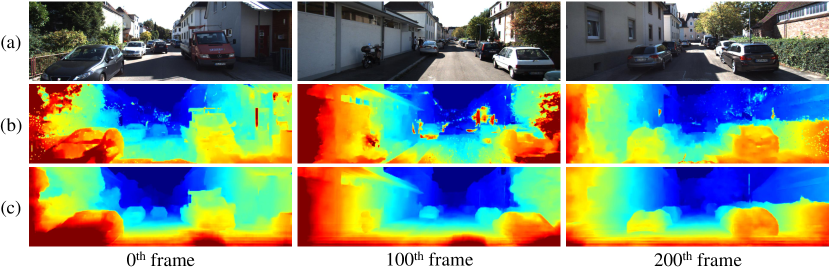
Figure 3: Disparity maps predicted using MADNet as the base network on the KITTI [9] sequence. (a) Left images, (b) MADNet with MAD adaptation [39], (c) Ours-MAD. with MAD adaptation. Red pixel values indicate closer objects.

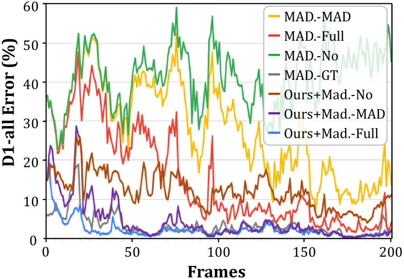
Figure 4: D1-all error (%) across frames in sequence from the KITTI [9] dataset with respect to the adaptation methods.

5.3.2 Convergence.

In Fig. 3, we evaluate the qualitative results related to the convergence analysis. The results contain good initialized parameters (first column), fast adaptation (second column), and convergence to low errors (last column) as analyzed above. As the adaptation proceeds, the MADNet (row 2) estimates better prediction, yet still shows a high error while Ours-MAD (row 3) shows not only robust initial performance but also faster convergence to low errors.

To analyze and compare the adaptation cost corresponding to the methods, we visualize the adaptation performance over frames of the sequence from the KITTI [9] dataset in Fig. 4. In overall view, the results show that our PointFix adapts faster than [39] and converges with lower errors regardless of the adaptation method. Furthermore, the comparison between MAD.-No (green) and Ours+Mad.-No (brown) shows the effectiveness of the initial base parameters. The comparison between MAD.-MAD (yellow) and Ours+Mad.-MAD (purple) shows that the performance is improved by PointFix with MAD adaptation, while MAD.-Full (red) overtakes from the about $100$-th frame. Finally, Ours+Mad.-Full (blue) adapts faster than all the other methods and converges to the low D1-all error, showing comparable performance with MAD.-GT (gray) fine-tuned with ground-truth. The additional experimental results and analysis are shown in supplementary material.

5.3.3 Comparison with domain generalization methods.

To argue the practicality of online stereo adaptation, we compare our model with the state-of-the-art domain generalization (DG) methods [44, 34, 23] that the stereo models are trained on the synthetic dataset and evaluated on the unseen real dataset without the additional adaptation.

Table 5: Comparisons of domain generalization methods and our method evaluated on the KITTI [9] dataset.

Method	Adapt.	D1-all	EPE	FPS
DSMNet [44]	N/A	1.59	0.68	1.30
CFNet [34]	N/A	1.93	0.97	4.27
Raft [23]	N/A	1.66	0.71	22.44
MADNet [39]	MAD	1.95	0.82	35.7
Ours-MAD.	MAD	1.47	0.70	35.7

For a fair comparison, the models are pretrained on the SceneFlow [25] dataset and evaluated on the KITTI [9] dataset. Note that we report the performance of our model measured under the long-term adaptation setting. As shown in Table 5, our model not only outperforms the generalization approaches in terms of D1-all error but also shows about $\times 27$, $\times 8.3$, and $\times 1.6$ faster inference speed than [44], [34], and [23], respectively, despite of additional adaptation steps. While the domain generalization approaches [44, 34, 23] estimate the depth maps without the adaptation, they require a large number of parameters to obtain a generalized stereo model, making them impractical. This is worth noting that our method has high applicability to the practical application such as autonomous driving in terms of accuracy and inference speed.

6 Conclusion

In this paper, we proposed PointFix, a novel meta-learning framework to effectively adapt any deep stereo models in online setting. Compared with previous online stereo adaptation approaches facing global domain bias problem to synthetic data, our model can induce maximal performance of the base stereo networks by the proposed the auxiliary network PointFixNet and learning-to-fix strategy, that can adapt well to the fine-grained domain gap. Our extensive experiments show PointFix achieves state-of-the-art results, outperforming several online stereo adaptation methods in a wide variety of environments. In addition, the results demonstrate that PointFix is capable of improving the generalization ability of the stereo models.

PointFix: Learning to Fix Domain Bias for Robust Online Stereo Adaptation
- Supplementary Materials -

Kwonyoung Kim¹  Jungin Park¹  Jiyoung Lee²
Dongbo Min³  Kwanghoon Sohn¹Corresponding author.

In this supplement, we provide the implementation details and the additional experimental results. First, we provide the training and adaptation details used in our experiments, and the network configuration of PointFixNet. To demonstrate the effectiveness of PointFix, we extend the experiments, including the convergence analysis, synthetic to synthetic scenarios, qualitative results and additional ablation studies, in the following section. The videos for the predicted disparity sequence (2011_09_30_drive_0027_sync of the KITTI [9] dataset) and the 3D reconstruction from the predicted disparity are provided in .mp4 format. Please refer our video supplementary files (‘Sim-to-Real.zip’).

7 Implementation Details

7.0.1 Additional datasets.

In this section, we introduce datasets used to conduct the additional experiments, including comparisons with domain generalization approaches in the main paper and synthetic to synthetic adaptation in this document. Specifically, we use the SceneFlow [25] dataset to train the models evaluated on comparisons with domain generalization methods [44, 34]. The SceneFlow is a synthetic dataset and contains 39,000 stereo frames with 960 $\times$ 540 pixel resolution. We use the FlyingThings3D (F3D) [25] dataset, which is one of the subsets of the SceneFlow dataset, only to train the models for the experiments in this supplement. In addition, we use the Virtual KITTI 2 [3] dataset as a test benchmark in Sec. 8.2, that contains photo-realistic and synthetic stereo images recreated from the KITTI [10] dataset. This dataset consists of 5 separate scenes corresponding to different locations and each scene is transformed to represent 6 different weather and lighting conditions (i.e., clone, fog, morning, overcast, rain, and sunset) for the same scene. Therefore, we use a total of 30 sequences for short-, mid-, and long-term adaptation. Each sequence consists of at least 233 frames and frame resolution is 1242 $\times$ 375.

7.0.2 Training.

In our experiments, we use TensorFlow library [1] and a single NVIDIA RTX A6000 48GB for training and NVIDIA TITAN RTX 24GB for inference. For the short-term experiment in the main paper, the test images of DrivingStereo [42] dataset are rescaled into 703$\times$320 for disparity range. For such a reason, we resize whole images in Synthia [32] dataset to half resolution as in [38]. All of initial parameters of base models are pretrained on the F3D dataset which is a synthetic dataset provided from [25]. Unless specified, we used the Synthia [32] dataset to train the base model with our method. For our model that uses the DispNetC [25] as the base network, we set the inner loop learning rates $\alpha$ and the outer loop learning rate $\beta$ to $10^{-4}$ during the first 40k iterations, and $\alpha=10^{-5}$ and $\beta=10^{-4}$ for the last 10k iterations. For the model that uses the MADNet [39] as the base network, we use $\alpha=10^{-5}$ and $\beta=10^{-4}$ during 30k iterations, respectively.

7.0.3 Online adaptation.

At inference, the parameters of the base network are continuously updated with the reconstruction loss. For models trained on Synthia [32], we set the adaptation learning rate to $10^{-4}$ for their best performance. For our model with the MADNet as the base network, the learning rate for short-term adaptation is set to $10^{-4}$ and $10^{-5}$ is given for the mid-term and long-term Full adaptation experiments. For models trained on the F3D [25] or SceneFlow [25], we set the adaptation learning rate to $10^{-5}$ and $10^{-4}$ for the Full adaptation and MAD adaptation, respectively.

We compute the reconstruction loss differently according to the base network and the adaptation method due to the different structures of the network and the adaptation strategy. Specifically, the reconstruction loss for the DispNet [25] is computed on the final predicted disparity map following [38]. The MADNet [39] with Full adaptation computes the reconstruction loss for all disparity maps at every single module, while a single disparity map is chosen for the reconstruction loss with the MAD adaptation by the strategy proposed in [39].

7.0.4 Network architecture.

As described in the main paper, our PointFixNet consists of two main modules: a feature extraction module and a point-wise prediction module. We depict the network configuration using the DispNetC [25] and the MADNet [39] as the base network in Table 6 and Table 7, respectively. The feature extraction module consists of three convolutional layers and the point-wise prediction module contains four fully-connected (FC) layers. Such lightweight model-agnostic architecture enables PointFixNet to be applied regardless of the base network and makes the base network maintain inference speed.

Table 6: Network configuration using DispNetC [25] as the base network.

DispNetC
Layer	Ch I/O	Input	Output
conv1	3 / 64	$I^{l},I^{r}$	$\text{feat1}^{l,r}$
conv2	64 / 128	$\text{feat1}^{l,r}$	$\mathbf{f}^{l,r}$
conv_redir	128 / 64	$\mathbf{f}^{l}$	feat_redir
corr	128 / 81	$\mathbf{f}^{l,r}$	$\mathbf{c}$
conv_3a	145 / 256	$\mathbf{c},\text{feat\_redir}$	feat3a
conv_3b	256 / 256	feat3a	feat3b
conv_4a	256 / 512	feat3b	feat4a
conv_4b	512 / 512	feat4a	feat4b
conv_5a	512 / 512	feat4b	feat5a
conv_5b	512 / 512	feat5a	feat5b
conv_6a	512 / 1024	feat5b	feat6a
conv_6b	1024 / 1024	feat6a	feat6b
pr6+loss6	1024 / 1	ifeat6	pr6
upconv5	1024 / 512	feat6b	upfeat5
iconv5	1024 / 512	upfeat5,pr6,feat5b	ifeat5
pr5+loss5	512 / 1	ifeat5	pr5
upconv4	512 / 256	feat5b	upfeat4
iconv4	769 / 256	upfeat4,pr5,feat4b	ifeat4
pr4+loss4	256 / 1	ifeat4	pr4
upconv3	256 / 128	feat4b	upfeat4
iconv3	385 / 128	upfeat3,pr4,feat3b	ifeat3
pr3+loss3	128 / 1	ifeat3	pr3
upconv2	128 / 64	feat3b	upfeat2
iconv2	193 / 64	$\text{upfeat2,pr3},\mathbf{f}^{l}$	ifeat2
pr2+loss2	64 / 1	ifeat2	pr2
upconv1	64 / 32	feat2b	upfeat1
iconv1	97 / 32	upfeat1,pr2,feat1b	ifeat1
pr1+loss1	32 / 1	ifeat1	pr1
PointFixNet: Feature Extraction Module
Layer	Ch I/O	Input	Output
conv1	5 / 32	$I^{l},\hat{d},d$	$\mathbf{z}^{1}$
conv2	32 / 64	$\mathbf{z}^{1}$	$\mathbf{z}^{2}$
conv3	64 / 128	$\mathbf{z}^{2}$	$\mathbf{z}^{c}$
PointFixNet: Point-wise Prediction Module
Layer	Ch I/O	Input	Output
concat.	64, 81 / 145	$\mathbf{c},\mathbf{f}^{l}$	$\mathbf{z}^{b}$
concat.	145, 128 / 273	$\mathbf{z}^{b}$, $\mathbf{z}^{c}$	$\Pi(\mathbf{z}^{b},\mathbf{z}^{c})$
FC1	273 / 273	$\Pi(\mathbf{z}^{b},\mathbf{z}^{c})_{ij}$	$\mathbf{x}^{1}_{ij}$
FC2	273 / 273	$\mathbf{x}^{1}_{ij}$	$\mathbf{x}^{2}_{ij}$
FC3	273 / 273	$\mathbf{x}^{2}_{ij}$	$\mathbf{x}^{3}_{ij}$
FC4	273 / 1	$\mathbf{x}^{3}_{ij}$	$r_{ij}$

Table 7: Network configuration using MADNet [39] as the base network.

MADNet: Feature Extractor
Layer	Ch I/O	Input	Output
conv1	3 / 16	$I^{l},I^{r}$	$\text{feat}_{0}$
conv2	16 / 16	feat1	$\text{feat}_{1}$
conv3	16 / 32	$\text{feat}_{1}$	$\text{feat}_{1\_1}$
conv4	32 / 32	$\text{feat}_{1\_1}$	$\text{feat}_{2}(\mathbf{f})$
conv5	32 / 64	$\text{feat}_{2}$	$\text{feat}_{2\_1}$
conv6	64 / 64	$\text{feat}_{2\_1}$	$\text{feat}_{3}$
conv7	64 / 96	$\text{feat}_{3}$	$\text{feat}_{3\_1}$
conv8	96 / 96	$\text{feat}_{3\_1}$	$\text{feat}_{4}$
conv9	96 / 128	$\text{feat}_{4}$	$\text{feat}_{4\_1}$
conv10	128 / 128	$\text{feat}_{4\_1}$	$\text{feat}_{5}$
conv11	128 / 192	$\text{feat}_{5}$	$\text{feat}_{5\_1}$
conv12	192 / 192	$\text{feat}_{5\_1}$	$\text{feat}_{6}$
MADNet: Stereo Estimation network
Layer	Ch I/O	Input	Output
conv1	C / 128	$D_{n+1},\text{feat}_{n}^{l,r}$	$\text{feat}_{1}^{\text{SE}}$
conv2	128 / 128	$\text{feat}_{1}^{\text{SE}}$	$\text{feat}_{2}^{\text{SE}}$
conv3	128 / 96	$\text{feat}_{2}^{\text{SE}}$	$\text{feat}_{3}^{\text{SE}}$
conv4	96 / 64	$\text{feat}_{3}^{\text{SE}}$	$\text{feat}_{4}^{\text{SE}}$
conv5	64 / 32	$\text{feat}_{4}^{\text{SE}}$	$\text{feat}_{5}^{\text{SE}}$
conv6	32 / 1	$\text{feat}_{5}^{\text{SE}}$	$D_{n}$
MADNet: Residual Refinement network
Layer	Ch I/O	Input	Output
conv1	C / 128	$\text{feat}_{n}^{l},D_{n}^{*}$	$\text{feat}_{1}^{\text{R}}$
conv2	128 / 128	$\text{feat}_{1}^{\text{R}}$	$\text{feat}_{2}^{\text{R}}$
conv3	128 / 128	$\text{feat}_{2}^{\text{R}}$	$\text{feat}_{3}^{\text{R}}$
conv4	128 / 96	$\text{feat}_{3}^{\text{R}}$	$\text{feat}_{4}^{\text{R}}$
conv4	96 / 64	$\text{feat}_{4}^{\text{R}}$	$\text{feat}_{5}^{\text{R}}$
conv5	64 / 32	$\text{feat}_{5}^{\text{R}}$	$\text{feat}_{6}^{\text{R}}$
conv6	32 / 1	$\text{feat}_{6}^{\text{R}}$	$R_{n}$
PointFixNet: Feature Extraction Module
Layer	Ch I/O	Input	Output
conv1	5 / 32	$I^{l},\hat{d},d$	$\mathbf{z}^{1}$
conv2	32 / 64	$\mathbf{z}^{1}$	$\mathbf{z}^{2}$
conv3	64 / 128	$\mathbf{z}^{2}$	$\mathbf{z}^{c}$
PointFixNet: Point-wise Prediction Module
Layer	Ch I/O	Input	Output
corr.	32, 32 / 81	$\mathbf{f}^{l,r}$	$\mathbf{c}$
concat.	32, 81 / 113	$\mathbf{c},\mathbf{f}^{l}$	$\mathbf{z}^{b}$
concat.	113, 128 / 241	$\mathbf{z}^{b}$, $\mathbf{z}^{c}$	$\Pi(\mathbf{z}^{b},\mathbf{z}^{c})$
FC1	241 / 241	$\Pi(\mathbf{z}^{b},\mathbf{z}^{c})_{ij}$	$\mathbf{x}^{1}_{ij}$
FC2	241 / 241	$\mathbf{x}^{1}_{ij}$	$\mathbf{x}^{2}_{ij}$
FC3	241 / 241	$\mathbf{x}^{2}_{ij}$	$\mathbf{x}^{3}_{ij}$
FC4	241 / 1	$\mathbf{x}^{3}_{ij}$	$r_{ij}$

8 Additional Results

To show the superiority of our model, we further provide experimental results. In Sec. 8.1, we first analyze the performance convergence of our PointFix and previous works [38, 39] by expanding experiments shown in Sec. 5.2 of the main paper. We also evaluate the online adaptation performance on the synthetic-to-synthetic adaptation setting using the F3D [25], Virtual KITTI [3] and Synthia [32] datasets in Sec. 8.2. Finally, we provide additional qualitative results in Sec. 8.3, including the qualitative comparisons with the online adaptation methods [38, 39] and domain generalization methods [44, 34] on the KITTI [9] dataset.

8.1 Convergence Analysis

8.1.1 Short-term adaptation.

To prove the incomparable stability of our method, we display the adaptation performance over frames as contrasted with the previous methods [39] that stand on the DispNetC [25] in a sequence from the KITTI [9] in Fig. 5. While Ours+Disp.-Full (blue) is slightly better than L2A+Disp.-Full (red) using full sequence for adaptation, the superior quality of the initial parameters of the base network using PointFix is presented in the comparison between L2A+Disp.-No (yellow) and Ours+Disp.-No (green). The result shows PointFix is more robust against new environmental changes, achieving better performance without the adaptation. Moreover, the method with full adaptation shows almost similar performance to Disp.-GT (gray) that is fine-tuned using the KITTI [10, 26] training sets. Note that the results using MADNet as the base network are shown in Fig. 4 of the main paper.

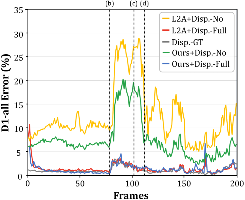
(a) D1-all error (%) across frames

(b) Input left image at 78th frame

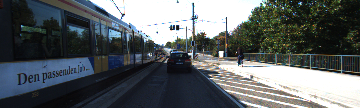
(c) Input left image at 103rd frame

(d) Input left image at 111st frame

Figure 5: (a) D1-all error (%) across frames in the sequence (2011_09_26_drive_101_sync) from the KITTI dataset with respect to the adaptation methods. (b) - (d) are input left images at section showing high error and it seems due to sudden changes in frames.

(a) Base network: MADNet

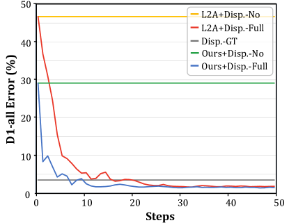
(b) Base network: DispNetC

Figure 6: Convergence analysis on a single frame with repetitive adaptation.

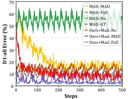
Base network: MADNet

Figure 7: Convergence analysis on a single sequence ‘2011_09_28_drive_0039_sync’ with repetitive adaptation.

8.1.2 Repetitive adaptation for single frame.

Furthermore, our PointFix takes advantage of the fast convergence. To validate the convergence speed, we repeatedly perform the adaptation for the first frame in a sequence from the KITTI and record D1-all errors for each adaptation step according to the base network. In Fig. 6(a), MAD.-No (green) and Ours+Mad.-No (brown) shows the performance of the initial base parameters trained using [39] and our PointFix. From each initial parameters, the drop rate of D1-all error represents the convergence speed of the adaptation. With the large margin, Ours+Mad.-Full (blue) achieves fast convergence and outperforms MAD.-Full (red) [39]. The result of Ours+Mad.-MAD (purple) also shows fast convergence and low error compared to MAD.-MAD (yellow). For DispNetC [25], we report the results on a single frame with repetitive adaptation in Fig. 6(b). The comparison between L2A+Disp.-Full (red) and Ours+Disp.-Full (blue) shows our PointFix converges faster than L2A [38], exceeding the model fine-tuned on groundtruth (gray) with only about 10 adaptation steps.

8.1.3 Repetitive adaptation for single sequence.

To conduct sequence-level convergence analysis, we perform repetitive adaptation on first 50 frames of the sequence from the KITTI dataset. As illustrated in Fig. 7, Ours+Mad.-MAD (purple) and Ours+Mad.-Full (light blue) converge with a small number of steps about 150 steps, while MAD.-MAD (yellow) and MAD.-Full (red) need about 250 steps to converge.

Table 8: Short-term and long-term adaptation performance evaluated on the Synthia [32] and Virtual KITTI 2 [3] datasets with models trained on the F3D [25] and Synthia [32] datasets.

Method	Adapt.	F3D $\rightarrow$ Synthia				F3D $\rightarrow$ VKITTI2				Synthia $\rightarrow$ VKITTI2
		Short-term		Long-term		Short-term		Long-term		Short-term		Long-term
		D1-all	EPE	D1-all	EPE	D1-all	EPE	D1-all	EPE	D1-all	EPE	D1-all	EPE
MADNet	No	48.49	20.86	48.00	20.39	47.91	17.62	47.13	17.09	46.95	13.36	42.29	9.30
Ours-MAD.	No	29.97	5.00	29.96	5.01	27.33	3.19	26.50	3.15	28.96	4.93	27.02	3.93
MADNet	Full	21.02	5.10	17.23	3.27	25.69	3.83	18.38	2.57	22.47	3.31	17.70	2.59
Ours-MAD.	Full	18.12	2.97	14.03	2.67	21.61	2.72	18.06	2.56	18.27	2.42	17.73	2.50
MADNet	MAD	19.98	4.12	18.20	3.58	23.90	3.12	18.55	2.62	29.29	5.53	18.66	2.55
Ours-MAD.	MAD	22.55	4.03	18.27	3.48	21.49	2.78	17.49	2.49	16.90	2.24	18.11	2.47

Table 9: Mid-term adaptation on the Virtual KITTI 2 [3] with models trained on the Synthia [32] dataset.

Method	Adapt.	clone		fog		morning		overcast		rain		sunset		Avg.
		D1-all	EPE	D1-all	EPE	D1-all	EPE	D1-all	EPE	D1-all	EPE	D1-all	EPE	D1-all	EPE
MADNet	No	33.25	7.90	69.62	14.57	33.86	7.60	34.25	7.92	48.38	9.72	34.39	8.07	42.29	9.30
Ours-MAD.	No	23.16	3.42	32.71	4.65	25.50	3.92	24.07	3.53	31.78	4.43	24.88	3.65	27.02	3.93
MADNet	Full	12.98	1.83	25.08	3.11	13.63	2.11	21.91	2.67	30.46	4.13	14.84	2.12	19.82	2.66
Ours-MAD.	Full	14.69	2.05	24.16	3.00	13.25	2.10	20.23	2.63	27.92	3.92	14.54	2.20	19.13	2.65
MADNet	MAD	19.32	2.58	32.03	4.03	16.56	2.33	23.74	2.92	30.79	4.26	18.96	2.44	23.57	3.09
Ours-MAD.	MAD	12.74	1.71	23.48	2.95	12.69	1.88	14.85	1.85	25.63	3.17	13.10	1.82	17.08	2.23

8.2 Synthetic to Synthetic Adaptation.

To verify the general adaptability of the proposed method in various scenarios that are not limited to synthetic-to-real, we further evaluate the performance under the short-, mid-, and long-term adaptation settings on several synthetic driving scene benchmarks. We present results according to the adaptation methods in Table 8 and Table 9.

In Table 8, we train the models on the F3D [25] or Synthia [32] datasets and evaluate the short- and long-term adaptation performance on the Synthia [32] or Virtual KITTI 2 [3] datasets. Note that each sequence for the short-term adaptation is defined as a distinct sequence provided from each dataset (e.g. SYNTHIA-SEQS-01-DAWN in the Synthia) and all frames are concatenated into a single sequence for the long-term adaptation. The comparison between the MADNet [39] and Ours-MAD. with No adaptation shows the initial parameters of our PointFix are extremely powerful to the new domain in terms of D1-all error and EPE on all datasets. The state-of-the-art performances using the adaptation are attained by our method except for one metric (i.e., D1-all error of the long-term adaptation on Synthia$\rightarrow$VKITTI2). The results evaluated on the Virtual KITTI 2 dataset indicates that the performances are different according to the training data. Since both the Synthia and Virtual KITTI 2 are driving scene datasets, the higher performance can be obtained when the models are trained on the Synthia than F3D.

To verify the robustness of our method under the mid-term adaptation setting, we evaluate the performance on various weather or lighting conditions using the Virtual KITTI 2 [3] dataset. Therefore, we provide the adaptation performance according to 6 different conditions and averaged performance. As shown in Table 9, our method consistently surpasses the baseline in all conditions, outperforming the MADNet with a large margin. Although the performance on the poor weather conditions (e.g. fog or rain) that have highly different pixel distributions from the training data shows relatively high error, the proposed method still outperforms the MADNet by $8.55\%$ and $5.16\%$ in terms of D1-all error, and $1.08$ and $1.09$ in terms of EPE for fog and rain sequences, respectively.

8.3 More qualitative results.

To argue the necessity of the online adaptation, we present the qualitative results of the proposed method compared to domain generalization (DG) approaches [44, 34]. We evaluate state-of-the-art DG models [44, 34] for all frames in the KITTI [9] dataset. In this experiment, we use the MADNet as the base network and perform the long-term adaptation. Fig. 8-(a) shows the performance in terms of D1-all error over all frames from the KITTI dataset. For the visibility of the results, we depict the performance corresponding to the $13600\sim 15000$th frame. As shown in the figure, Ours-MAD. (green) achieves lower error rate than DSMNet [44] (blue) and CFNet [34] (orange). In addition, we depict input left frames showing high error rates on the DG methods, as shown in Fig. 8(b)-(d). Although the scene is not abruptly changed or the intensity of illumination is not drastically changed, the DG methods often show remarkably low performance compared with our method, which has stable performance in overall frames. Thus, the fast inference speed and robust performance in novel environments make our method more practical to real-world applications.

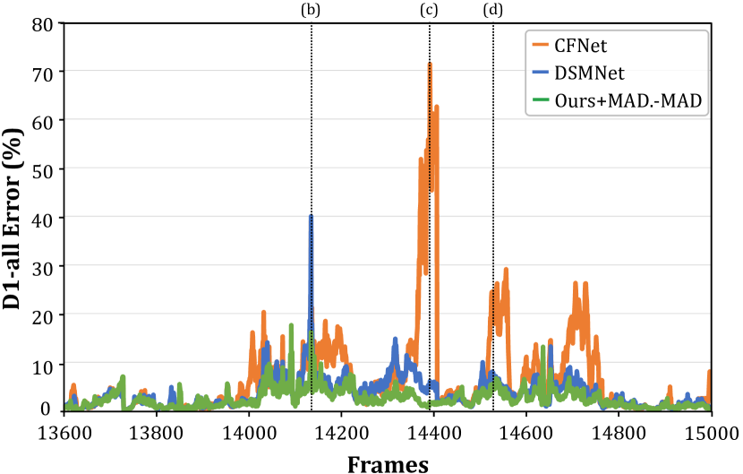
(a) D1-all error (%) across frames

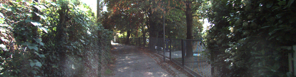
(b) Input left image at 14150th frame

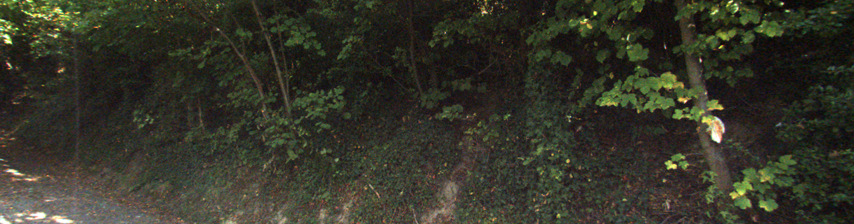
(c) Input left image at 14414th frame

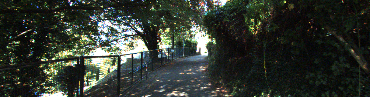
(d) Input left image at 14551st frame

Figure 8: (a) D1-all error (%) across frames in the consecutive sequences including ‘2011_09_26_drive_0086_sync’ (frames in (b) and (c)) and ‘2011_09_26_drive_0087_sync’ (frame in (d)) from the KITTI [9] dataset with respect to the adaptation methods. (b) - (d) are input left images at section showing high error and it seems due to sudden changes in frames.

In Fig. 9, we present more qualitative results evaluated on the sequence from the KITTI dataset according to the base network and the adaptation method. The results contain the quality of the initialized parameters(first column), fast adaptation (second column), and convergence to low errors (last column). For the comparison between methods with no adaptation (b)-(e), our PointFix shows visually better results at the inner or boundary of objects regardless of the base network. The comparison between the results in the second column, $\mathbf{L2A-Disp.Full}$ (f), $\mathbf{Ours-Disp.Full}$ (h), $\mathbf{Ours-MAD.Full}$ (i), and $\mathbf{Ours-MAD.MAD}$ (k) show the superior performance with only 50 adaptation steps. The results in the third column, our PointFix converges to the low error, showing clear prediction on the inner and boundary of objects.

8.4 Additional ablation studies

Table 10: Ablation studies for various components. All results are obtained using Full adaptation on short-term sequences.

Method	D1-all	EPE
No PointFixNet (w/ selection)	7.77	2.02
No residual learning	2.10	0.82
Point selection threshold 1	1.97	0.80
Point selection threshold 5	2.01	0.80
No online ML	5.53	1.13
Ours-MAD.	2.00	0.74

8.4.1 Ablation study on PointFixNet.

To further verify the effectiveness of PointFixNet, we ablate PointFixNet while keeping the point selection process. As shown in Table 10(row 1), the model trained using the sparse loss without PointFixNet records the poor performance.

8.4.2 Ablation study on residual learning.

We adopted residual learning to make back-propagation flow through skip connection. The performance without residual learning shown in Table 10(row 2) degrades slightly compared to model trained with residual learning(row 6).

8.4.3 Ablation study on point selection threshold.

We choose 3 pixels error as threshold for point selection motivated by the bad3 metric. As shown in Table 10(row 3,4 and 6), the best performance in terms of EPE is attained with 3 pixels.

8.4.4 Ablation study on online meta-learning.

We adopted online meta-learning framework to jointly train PointFixNet and the base network. The performance of offline meta-learning is shown in Table 10(row 5) indicating the advantage of online meta-learning in our framework.

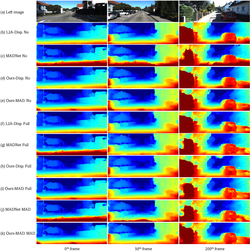
Figure 9: Disparity maps predicted using MADNet and DispNet as the base network on the KITTI sequence [9]. (a) Input left images; predicted disparity with (b)-(e) no adaptation; (f)-(i) full adaptation; and (j), (k) MAD adaptation.

References

- [1] Abadi, M., Agarwal, A., Barham, P., Brevdo, E., Chen, Z., Citro, C., Corrado, G.S., Davis, A., Dean, J., Devin, M., Ghemawat, S., Goodfellow, I., Harp, A., Irving, G., Isard, M., Jia, Y., Jozefowicz, R., Kaiser, L., Kudlur, M., Levenberg, J., Mané, D., Monga, R., Moore, S., Murray, D., Olah, C., Schuster, M., Shlens, J., Steiner, B., Sutskever, I., Talwar, K., Tucker, P., Vanhoucke, V., Vasudevan, V., Viégas, F., Vinyals, O., Warden, P., Wattenberg, M., Wicke, M., Yu, Y., Zheng, X.: TensorFlow: Large-scale machine learning on heterogeneous systems (2015), https://www.tensorflow.org/, software available from tensorflow.org
- [2] Achtelik, M., Bachrach, A., He, R., Prentice, S., Roy, N.: Stereo vision and laser odometry for autonomous helicopters in gps-denied indoor environments. In: SPIE Defense, Security, and Sensing pp. 733219–733219 (2009)
- [3] Cabon, Y., Murray, N., Humenberger, M.: Virtual kitti 2. arXiv preprint arXiv:2001.10773 (2020)
- [4] Chang, J.R., Chen, Y.S.: Pyramid stereo matching network. In: CVPR (2018)
- [5] Chen, Y., Van Gool, L., Schmid, C., Sminchisescu, C.: Consistency guided scene flow estimation. In: ECCV (2020)
- [6] Finn, C., Abbeel, P., Levine, S.: Model-agnostic meta-learning for fast adaptation of deep networks. In: PMLR (2017)
- [7] Finn, C., Rajeswaran, A., Kakade, S., Levine, S.: Online meta-learning. In: ICML (2019)
- [8] Garg, R., Bg, V.K., Carneiro, G., Reid, I.: Unsupervised cnn for single view depth estimation: Geometry to the rescue. In: ECCV (2016)
- [9] Geiger, A., Lenz, P., Stiller, C., Urtasun, R.: Vision meets robotics: The kitti dataset. Int. J. of Rob. Res. 32(11), 1231–1237 (2013)
- [10] Geiger, A., Lenz, P., Urtasun, R.: Are we ready for autonomous driving? the kitti vision benchmark suite. In: CVPR (2012)
- [11] Geiger, A., Roser, M., Urtasun, R.: Efficient large-scale stereo matching. In: ACCV (2010)
- [12] Godard, C., Mac Aodha, O., Brostow, G.J.: Unsupervised monocular depth estimation with left-right consistency. In: CVPR (2017)
- [13] Hirschmuller, H.: Stereo processing by semiglobal matching and mutual information. IEEE Trans. Pattern Anal. Mach. Intell. 30(2), 328–341 (2008)
- [14] Hoffman, J., Wang, D., Yu, F., Darrell, T.: Fcns in the wild: Pixel-level adversarial and constraint-based adaptation. arXiv preprint arXiv:1612.02649 (2016)
- [15] Hu, X., Mordohai, P.: A quantitative evaluation of confidence measures for stereo vision. IEEE Trans. Pattern Anal. Mach. Intell. 34(11), 2121–2133 (2012)
- [16] Kendall, A., Martirosyan, H., Dasgupta, S., Henry, P., Kennedy, R., Bachrach, A., Bry, A.: End-to-end learning of geometry and context for deep stereo regression. In: ICCV (2017)
- [17] Khamis, S., Fanello, S., Rhemann, C., Kowdle, A., Valentin, J., Izadi, S.: Stereonet: Guided hierarchical refinement for real-time edge-aware depth prediction. In: ECCV (2018)
- [18] Kim, S., Kim, S., Min, D., Sohn, K.: Laf-net: Locally adaptive fusion networks for stereo confidence estimation. In: CVPR (2019)
- [19] Kim, S., Min, D., Kim, S., Sohn, K.: Unified confidence estimation networks for robust stereo matching. IEEE Trans. Image Process. 28(3), 1299–1313 (2018)
- [20] Kirillov, A., Wu, Y., He, K., Girshick, R.: Pointrend: Image segmentation as rendering. In: CVPR (2020)
- [21] Knowles, M., Peretroukhin, V., Greene, W.N., Roy, N.: Toward robust and efficient online adaptation for deep stereo depth estimation. In: ICRA (2021)
- [22] Li, D., Hospedales, T.: Online meta-learning for multi-source and semi-supervised domain adaptation. In: ECCV (2020)
- [23] Lipson, L., Teed, Z., Deng, J.: Raft-stereo: Multilevel recurrent field transforms for stereo matching. In: 3DV (2021)
- [24] Liu, M.Y., Tuzel, O.: Coupled generative adversarial networks. In: NIPS (2016)
- [25] Mayer, N., Ilg, E., Häusser, P., Fischer, P., Cremers, D., Dosovitskiy, A., Brox, T.: A large dataset to train convolutional networks for disparity, optical flow, and scene flow estimation. In: CVPR (2016)
- [26] Menze, M., Geiger, A.: Object scene flow for autonomous vehicles. In: CVPR (2015)
- [27] Mnih, V., Kavukcuoglu, K., Silver, D., Rusu, A.A., Veness, J., Bellemare, M.G., Graves, A., Riedmiller, M., Fidjeland, A.K., Ostrovski, G., et al.: Human-level control through deep reinforcement learning. Nature 518(7540), 529–533 (2015)
- [28] Pang, J., Sun, W., Yang, C., Ren, J., Xiao, R., Zeng, J., Lin, L.: Zoom and learn: Generalizing deep stereo matching to novel domains. In: CVPR (2018)
- [29] Patricia, N., Carlucci, F.M., Caputo, B.: Deep depth domain adaptation: A case study. In: ICCV (2017)
- [30] Poggi, M., Kim, S., Tosi, F., Kim, S., Aleotti, F., Min, D., Sohn, K., Mattoccia, S.: On the confidence of stereo matching in a deep-learning era: a quantitative evaluation. IEEE Trans. Pattern Anal. Mach. Intell. (2021)
- [31] Poggi, M., Tonioni, A., Tosi, F., Mattoccia, S., Di Stefano, L.: Continual adaptation for deep stereo. IEEE Trans. Pattern Anal. Mach. Intell. pp. 1–1 (2021)
- [32] Ros, G., Sellart, L., Materzynska, J., Vazquez, D., Lopez, A.M.: The synthia dataset: A large collection of synthetic images for semantic segmentation of urban scenes. In: CVPR (2016)
- [33] Rusu, A.A., Rabinowitz, N.C., Desjardins, G., Soyer, H., Kirkpatrick, J., Kavukcuoglu, K., Pascanu, R., Hadsell, R.: Progressive neural networks. arXiv preprint arXiv:1606.04671 (2016)
- [34] Shen, Z., Dai, Y., Rao, Z.: Cfnet: Cascade and fused cost volume for robust stereo matching. In: CVPR (2021)
- [35] Sun, D., Yang, X., Liu, M.Y., Kautz, J.: Pwc-net: Cnns for optical flow using pyramid, warping, and cost volume. In: CVPR (2018)
- [36] Tankovich, V., Hane, C., Zhang, Y., Kowdle, A., Fanello, S., Bouaziz, S.: Hitnet: Hierarchical iterative tile refinement network for real-time stereo matching. In: CVPR (2021)
- [37] Tonioni, A., Poggi, M., Mattoccia, S., Di Stefano, L.: Unsupervised adaptation for deep stereo. In: ICCV (2017)
- [38] Tonioni, A., Rahnama, O., Joy, T., Stefano, L.D., Ajanthan, T., Torr, P.H.: Learning to adapt for stereo. In: CVPR (2019)
- [39] Tonioni, A., Tosi, F., Poggi, M., Mattoccia, S., Stefano, L.D.: Real-time self-adaptive deep stereo. In: CVPR (2019)
- [40] Tosi, F., Poggi, M., Mattoccia, S., Tonioni, A., di Stefano, L.: Learning confidence measures in the wild. BMVC (2017)
- [41] Wang, H., Wang, X., Song, J., Lei, J., Song, M.: Faster self-adaptive deep stereo. In: ACCV (2020)
- [42] Yang, G., Song, X., Huang, C., Deng, Z., Shi, J., Zhou, B.: Drivingstereo: A large-scale dataset for stereo matching in autonomous driving scenarios. In: CVPR (2019)
- [43] Zbontar, J., LeCun, Y., et al.: Stereo matching by training a convolutional neural network to compare image patches. J. Mach. Learn. Res. 17(1), 2287–2318 (2016)
- [44] Zhang, Qi, X., Yang, R., Prisacariu, V., Wah, B., Torr, P.: Domain-invariant stereo matching networks. In: ECCV (2020)
- [45] Zhang, K., Lu, J., Lafruit, G.: Cross-based local stereo matching using orthogonal integral images. IEEE Trans. Circuit Syst. Video Technol. 19(7), 1073–1079 (2009)
- [46] Zhang, Y., Khamis, S., Rhemann, C., Valentin, J., Kowdle, A., Tankovich, V., Schoenberg, M., Izadi, S., Funkhouser, T., Fanello, S.: Activestereonet: End-to-end self-supervised learning for active stereo systems. In: ECCV (2018)
- [47] Zhang, Z., Lathuilière, S., Pilzer, A., Sebe, N., Ricci, E., Yang, J.: Online adaptation through meta-learning for stereo depth estimation. arXiv preprint arXiv:1904.08462 (2019)
- [48] Zhou, C., Zhang, H., Shen, X., Jia, J.: Unsupervised learning of stereo matching. In: ICCV (2017)