Gaia: Graph Neural Network with Temporal Shift aware Attention for Gross Merchandise Value Forecast in E-commerce

Abstract

E-commerce has gone a long way in empowering merchants through the internet. In order to store the goods efficiently and arrange the marketing resource properly, it is important for them to make the accurate gross merchandise value (GMV) prediction. However, it’s nontrivial to make accurate prediction with the deficiency of digitized data. In this article, we present a solution to better forecast GMV inside Alipay app. Thanks to graph neural networks (GNN) which has great ability to correlate different entities to enrich information, we propose Gaia, a graph neural network (GNN) model with temporal shift aware attention. Gaia leverages the relevant e-seller’ sales information and learn neighbor correlation based on temporal dependencies. By testing on Alipay’s real dataset and comparing with other baselines, Gaia has shown the best performance. And Gaia is deployed in the simulated online environment, which also achieves great improvement compared with baselines.

I Introduction

With the ever increasing use of the internet, a wide range of small and large companies have leveraged e-commerce to bolster sales. Aiming at the sale estimation for each merchant, the forecasting of gross merchandise value (GMV), which estimates the total sales volume over a period of time, has been playing an increasingly important role in e-commerce scenarios [1, 2]. In addition, a precise prediction has the potential of refraining from unexpected issues for profit loss, e.g., stockout, staff inefficiency and customer loss.

Intuitively, the GMV forecasting task could be formulated as a regression problem with time series analysis, which have been widely explored in numerous studies, including classical statistical method (e.g., AR [3] and ARIMA [3]) and recently emerging deep learning based methods (e.g., LSTM [4] and LSTNet [5]). Unfortunately, the capability of these approaches in time series forecasting may be distant from optimal or even satisfactory, due to the inevitable temporal deficiency issue in practical e-commerce scenarios. Empirically, the skew distribution shown in Fig 1(a) gives the strong evidence that only limited temporal information of e-sellers could be obtained for GMV forecasting, which severely hinders the performance of conventional time series forecasting method.

Besides, the GMV of e-sellers relies heavily on their supply chain enterprises [6]. This makes graph neural networks (GNNs) suitable for GMV forcasting for its ability of both utilizing neighbor information and time series dependencies. In addition, we observe another characteristic of GMV series in the e-commerce scenario, which we call temporal shift. We find two kinds of time shifts in GMV series. One is the self-shift, meaning that the GMV series may show similar patterns after an interval. For example, the GMV of a seller who sells seasonal goods may be similar as its historical GMV in the same season [1]. Another is inter-seller shift, e.g. for supply-chain relationships, the GMV of a seller will emerge a rising or decreasing pattern earlier than its downstream retailers, as retailers will firstly buy goods from its suppliers then retail to the customers. Though some GNN-based methods [7, 8, 9] have been proposed for GMV forcasting, they fail to make full use of time shift information in the e-commerce scenario.

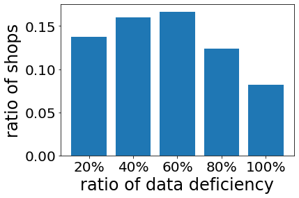
(a)

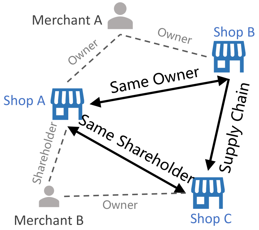
(b)

Figure 1: (a) illustrates the temporal deficiency problem, (b) shows a toy example of e-seller graph, only the blue nodes and the solid line edges exist in the final graph.

We hereby propose Gaia, a Graph Neural Network with Tempoal Shift aware Attention. To solve the temporal deficiency problem, we mine different relationships among shops and establish a shop network, making up for the information loss. Our model contains three basic components: Feature Fusion Layer (FFL), Temporal Embedding Layer (TEL) and an Inter and intra Temporal shift Aware Attention mechanism for classical Graph Convolutional Network (short as ITA-GCN). The FFL is in charge of combining basic features and GMV series of a shop, TEL aims at extracting temporal patterns, and the ITA-GCN is well-designed to caputure the Temporal Shift patterns not only from the time series of an individual shop, but also from its neighbors.

Our main contribution is listed as follows:

• In the e-commerce scenario, we propose Gaia, a GMV forecasting framework, which aims at solving the temporal deficiency problem and the temporal shift problem of e-sellers.

• Our proposal not only fuses auxiliary features with time series features of a e-seller via a FFL and a TEL, but also learns temporal shift patterns from its own and its neighbors’ GMV sequence, via a ITA-GCN.

• We conduct extensive experiments on real-world data set and also deploy Gaia in online environment, both the offline and online results show that Gaia outperforms all state of the art methods.

II Related Work

In past decades, time series analysis based methods have been well studied [10]. Due to the simplicity and interpretability, early works mainly focus on statistical modelling based on a assumption of stationary process [3]. Particularly, the ARIMA approach and its variants (e.g., AR, MA, and ARMA) have shown powerful capability in various applications [3], which make prediction only by the linear combination of historical values, i.e., so-called univariate time series analysis. On the comparison, attention is natually shifting towards multivariate time series analysis and a series of approaches [11] are proposed to inherently characterize interdependencies among variables. However, the prefabricated assumption and model complexity are bottlenecks. Due to the powerful ability of feature interaction, deep neural networks are introduced to capture non-linear patterns in time series. Following this line, DeepAR [12] and LogTrans [13] are respectively developed for univariate time series prediction based on deep probabilistic models and the recently emerging Transformer architecture. Meanwhile, to marry the strength of convolutional neural networks (CNNs) and recurrent neural networks (RNNs), numerous methods [5, 14, 15] are proposed to capture local and global dependencies among variables for multivariate time series prediction. Unfortunately, the inevitable temporal deficiency issue in practical e-commerce scenarios still threatens the capbility of current methods.

As a prevailing paradigm, graph neural networks (GNNs) has shown the remarkable strength for ingesting valuable information encoded in graph-structured data [16, 17, 18, 19, 20]. In line with the main focus in our paper, we center on the well studied spatial-temporal GNNs (STGNNs) which initially designed to the traffic prediction task [7, 9, 21]. In general, a STGNN is comprised of two main components: a graph convolution capturing spatial structure and a deep architecture dealing with time series on nodes through CNNs [22, 7] and RNNs[23, 24, 25]. Distinct from above paradigm based on pre-defined graph structure, a few efforts [8, 26] have been made for simultaneously learning a graph structure and a powerful GNN for time series prediction in an unified framework. Nevertheless, these methods still neglect the temporal shift issues. In contrast, our proposed Gaia hinges on a well-designed graph convolutional component, which carefully considers the temporal shift in both inter and intra level. In addition, node-level feature learning is also achieved in a more fine-grained manner through feature fusion and temporal embedding.

III Preliminaries

III-A Problem Definition

This paper addresses the problem of forecasting GMV of e-sellers. Suppose there exists an e-seller graph $\mathcal{G}=(\mathcal{V},\mathcal{E})$ consisting of $N$ e-sellers as node set $\mathcal{V}=\{v_{1},\ldots,v_{N}\}$, and $M$ links between these e-sellers as edge set $\mathcal{E}=\{e_{1},\ldots,e_{M}\}$. For each e-seller $v$, let $\bm{z}_{v}\in\mathbb{R}_{+}^{T}$ denote its monthly GMV, where $T$ is the number of time steps. We assume that each e-seller have both temporal and static auxiliary features (detail description in Section IV-A), which can be denoted as $\mathbf{F}^{\mathcal{T}}_{v}=\{\bm{f}^{\mathcal{T}}_{v,t}\}_{t=1}^{T}\in\mathbb{R}^{T\times D^{\mathcal{T}}}$ and $\bm{f}^{\mathcal{S}}_{v}\in\mathbb{R}^{D^{\mathcal{S}}}$, respectively. Given the above information, the problem is to predict the future GMV of $T^{\prime}$ months for each e-seller $v$, which can be denoted as $\bm{y}_{v}\in\mathbb{R}_{+}^{T^{\prime}}$.

III-B E-Seller Graph Construction

In the scenario of e-commerce, there exists two kinds of relationships between e-sellers that can improve the effectiveness of GMV forecasting. Fig 1(b) shows a demonstration of these two relationships. The first relationship is supply chain relationship, in which one associated e-seller sells its goods to another e-seller, and the upstream e-seller’s GMV is affected by the downstream e-seller. The GMV traded by adjacent e-sellers in a supply chain is usually correlated. For example, a downstream e-seller with an increased GMV may need more raw materials to produce more goods. This may lead to an increase in orders from its upstream suppliers, thus increase the GMV of upstream e-sellers to a certain extent. The second one is same owner/shareholder relationship. Since two e-sellers that share the same owners or shareholders usually have similar operation strategies, such as similar willingness to participate in shopping festivals, their GMVs may share a common trend.

These two kinds of relationships make up the edge set of e-seller graph. Note that, the e-seller consists of only shops as nodes, and the edges type is made as one of the edge features, so the graph here is considered a homogenous graph.

IV Methodology

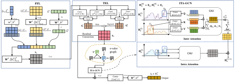
Figure 2: Overview of Gaia, which consists of three main components: Feature Fusion Layer (FFL), Temporal Embedding Layer (TEL) and Inter and intra Temporal shift aware Attention based Graph Convolutional Network (ITA-GCN). FFL first fuses auxiliary features with the GMV series at a single timestamp. Then TEL models the temporal patterns along the timeline. Finally, with an well-designed convolutional attention unit, ITA-GCN learns the temporal shift on the structured e-seller graph.

The overview of Gaia is depicted in Fig. 2.

IV-A Feature Fusion Layer

In the industrial scenario of e-commerce, an e-seller is usually characterized via various features. Here, for each e-seller node $v$, we summarize following features:

• $\{z_{v,t}\}^{T}_{t=1}$: historical monthly GMV series.

• $\bm{f}^{\mathcal{T}}_{v,t}\in\mathbb{R}^{D^{\mathcal{T}}}$: auxiliary temporal features at each time $t\in[1,2,\cdots,T]$, e.g., the month, the monthly amount of customers and orders.

• $\bm{f}^{\mathcal{S}}_{v}\in\mathbb{R}^{D^{\mathcal{S}}}$: auxiliary static features, e.g., the industry, the registration location.

Intuitively, both the individual time series and auxiliary temporal/static features could help Gaia better understand the intrinsic change trend of GMV for each e-seller. For better representation, we equip Gaia with a Feature Fusion Layer to fuse available features in a more fine-grained manner. Formally, given an e-seller $v$ at time t, the FFL firstly projects aforementioned features (i.e., $z_{v,t},\bm{f}^{\mathcal{T}}_{v,t}$ and $\bm{f}^{\mathcal{S}}_{v}$ ) to the $C$-dimensional embedding space, followed by a concatenation and a fully-connected layer for feature fusion.

$$\small\tilde{\bm{z}}_{v,t} =z_{v,t}\cdot\bm{w}^{\mathcal{I}}+\bm{b}^{\mathcal{I}},$$ (1)

$$\tilde{\bm{f}}^{\mathcal{T}}_{v,t} =\mathbf{W}^{\mathcal{T}}\bm{f}_{v,t}^{\mathcal{T}}+\bm{b}^{\mathcal{T}}_{t},$$ (2)

$$\tilde{\bm{f}}_{v}^{\mathcal{S}} =\mathbf{W}^{\mathcal{S}}\bm{f}_{v}^{\mathcal{S}}+\bm{b}^{\mathcal{S}},$$ (3)

$$\bm{s}_{v,t} =\mathbf{W}^{\mathcal{F}}[\tilde{\bm{z}}_{v,t}\ ||\ \tilde{\bm{f}}_{v,t}^{\mathcal{T}}\ ||\ \tilde{\bm{f}}_{v}^{\mathcal{S}}]+\bm{b}^{\mathcal{F}}_{t},$$ (4)

where $\bm{w}^{\mathcal{I}}\in\mathbb{R}^{C}$, $\bm{b}^{\mathcal{I}}\in\mathbb{R}^{C}$, $\mathbf{W}^{\mathcal{T}}\in\mathbb{R}^{C\times D^{\mathcal{T}}}$, $\{\bm{b}^{\mathcal{T}}_{t}\in\mathbb{R}^{C}\}_{t=1}^{T}$, $\mathbf{W}^{\mathcal{S}}\in\mathbb{R}^{C\times D^{\mathcal{S}}}$, $\bm{b}^{\mathcal{S}}\in\mathbb{R}^{C}$, $\mathbf{W}^{\mathcal{F}}\in\mathbb{R}^{C\times 3C}$ and $\{\bm{b}^{\mathcal{F}}_{t}\in\mathbb{R}^{C}\}_{t=1}^{T}$ are learnable parameters, “$||$” is the concatenation operator.

IV-B Temporal Embedding Layer

As mentioned above, the FFL endows Gaia with powerful capability for subtle feature fusion at each single timestamp, whereas the feature interaction along the timeline is not carefully considered, which potentially implies the various temporal patterns (e.g., annual and seasonal patterns) derived from GMV series. Therefore, inspired by the idea of  [26], we develop the Temporal Embedding Layer (TEL) based on coupled temporal convolution layers, where a temporal convolution layer is in charge of temporal patterns extraction, paired with another temporal convolution layer for information denoising. Specifically, given an input GMV series for e-seller $v$ (i.e., $\{z_{v,t}\}^{T}_{t=1}$), we could obtain the fused features at each time step through the FFL, denoted as temporal feature matrix $\mathbf{S}_{v}=\{\bm{s}_{v,t}\}_{t=1}^{T}\in\mathbb{R}^{T\times C}$. Following common strategies in [27, 28], we define a group of kernels with size $\{(2^{k}\times C;C/{K})\}_{k=1}^{K}$, which aim at capturing temporal patterns in multiple levels. Here, $\{a\times b;c\}$ means a subgroup of $c$ kernels with size $\{a\times b\}$. Then, the coupled temporal convolution layers work as follows:

$$\small\mathbf{S}_{v}^{\mathcal{C}}=[\mathbf{L}_{\{2\times C;C/K\}}^{\mathcal{C},1}\star\mathbf{S}_{v}\ ||\ \cdots\ ||\ \mathbf{L}_{\{2^{K}\times C;C/K\}}^{\mathcal{C},K}\star\mathbf{S}_{v}],$$ (5)

$$\mathbf{S}_{v}^{\mathcal{D}}=[\mathbf{L}_{\{2\times C;C/K\}}^{\mathcal{D},1}\star\mathbf{S}_{v}\ ||\ \cdots\ ||\ \mathbf{L}_{\{2^{K}\times C;C/K\}}^{\mathcal{D},K}\star\mathbf{S}_{v}],$$ (6)

where $\mathbf{L}^{\mathcal{C},k}_{\{a\times b;c\}}$ and $\mathbf{L}^{\mathcal{D},k}_{\{a\times b;c\}}$ means the $k$^th temporal convolution consisting of $c$ kernels with size $\{a\times b\}$ for temporal pattern capturing and information denoising, respectively, and $\star$ is the 1D convolution operator with zeros padding.

Clearly, above temporal convolution layers provide coupled valuable matrices, where the former (i.e., $\mathbf{S}_{v}^{\mathcal{C}}\in\mathbb{R}^{T\times C}$ ) preserves multi-level temporal patterns derived from GMV series while the latter (i.e., $\mathbf{S}_{v}^{\mathcal{D}}\in\mathbb{R}^{T\times C}$ ) emphasizes important/relevant patterns. Subsequently, the TEL gives the final temporal representation for e-seller $v$ as follows:

$$\mathbf{E}_{v}=\text{ReLU}(\mathbf{S}_{v}^{\mathcal{C}})\odot\text{Sigmoid}(\mathbf{S}_{v}^{\mathcal{D}}),$$ (7)

where $\odot$ denotes the Hadamard product.

IV-C Inter and Intra Temporal shift Aware Attention based Graph Neural Network

In this section, we are devoted to learning structural information from the well-established e-seller graph to benefit GMV forecasting. As mentioned above, we should pay careful attention to following two temporal shift issues in e-commerce scenarios, which could be hardly captured by current graph neural networks:

• Inter temporal shift among two connected e-sellers. Generally, different types of e-seller (i.e., suppliers and retailers) have different response times to market trends, e.g., the GMV of suppliers usually increase/decrease several months before retailers. Moreover, a center e-seller in the graph may place different importances to its neighbors, where neighbors with rich series are expected to be emphasized.

• Intra temporal shift existed in individual e-seller. Intuitively, the GMV of a certain e-seller is directed related to time and varies with seasons, i.e., the GMV of a e-seller selling air conditioners always a sharp rise in summer. Such a periodic shift is essential to accurately summarize historical GMV series for each individual shop.

In light of these findings, we prepare a well-designed Inter and intra Temporal shift aware Attention mechanism for classical Graph Convolutional Network (short as ITA-GCN) to tackle the above issues.

IV-C1 Convolutional Attention Unit

As the heart of ITA mechanism, Convolutional Attention Unit (short as CAU), based on recently emerging self-attention architecture [29], aims at capturing temporal shift for arbitrary edge $v\rightarrow u$ ($u$ and $v$ could be the same). In other words, the CAU learns temporal attention weights over timestamps conditioned on paired GMV series. Given an edge $v\rightarrow u$, the CAU produce the final representation that summarize the influence of temporal shift from $v$ to $u$ as follows:

$$\small\mathbf{Q}_{u} = \mathbf{L}_{\{3\times C;C\}}^{Q}\star\mathbf{H}_{u},$$

$$\mathbf{K}_{v} = \mathbf{L}_{\{3\times C;C\}}^{K}\star\mathbf{H}_{v},$$

$$\mathbf{V}_{v} = \mathbf{L}_{\{1\times C;C\}}^{V}\star\mathbf{H}_{v},$$

$$\mathrm{CAU}(\mathbf{H}_{u},\mathbf{H}_{v}) = \mathrm{softmax}(\frac{\mathbf{Q}_{u}\mathbf{K}^{\top}_{v}}{\sqrt{C}}+\mathbf{M})\ \mathbf{V}_{v}$$

where $\mathbf{H}_{u},\mathbf{H}_{v}\in\mathbb{R}^{T\times C}$ is temporal representation for node $u$ and $v$, respectively. It is worthwhile that convolutional kernels (i.e., $\mathbf{L}^{Q},\mathbf{L}^{K},\mathbf{L}^{V}$) are incorporated to help CAU be aware of locality [13] of GMV series so that relevant features based on the shape of several adjacent points could be correctly matched. Moreover, we employ a mask matrix $\mathbf{M}\in\{-\infty,0\}^{T\times T}$ for filtering out rightward attention in order to avoid future information leakage.

IV-C2 ITA-GCN layer

Next, we build upon the architecture of graph attention network [18] to recursively obtain center node’s representation by aggregating its neighbors on e-seller graphs. Moreover, attentive weights of aggregation are generated to distinguish influence of temporal shift passed by connectivity. Here, we begin with a single layer, which produces representation for center node $\mathbf{H}_{u}^{(l+1)}$ by capturing i) inter temporal shift from influences of its neighbors and ii) intra temporal shift from its historical GMV series through our CAU component.

$$\small\mathbf{H}_{u}^{(l+1)}=\underbrace{\sum_{v\in N(u)}\alpha_{u,v}^{(l)}\mathrm{CAU}(\mathbf{H}_{u}^{(l)},\mathbf{H}_{v}^{(l)})}_{\text{Inter Neighbor Attention}}+\underbrace{\mathrm{CAU}(\mathbf{H}_{u}^{(l)},\mathbf{H}_{u}^{(l)})}_{\text{Intra Self Attention}},$$ (8)

where $N(u)$ is the neighbor set of node $u$, $\mathbf{H}_{u}^{(l)}$ and $\mathbf{H}_{v}^{(l)}$ is the representation of $l$-th ITA-GCN layer for node $u$ and $v$ respectively, which is initialized with the output of TEL, i.e., $\mathbf{H}_{u}^{(0)}=\mathbf{E}_{u}$ and $\mathbf{H}_{v}^{(0)}=\mathbf{E}_{v}$. Moreover, $\alpha_{u,v}^{(l)}$ controls how much information being aggregated on edge “$u\leftarrow v$”, which is implemented as follows:

$$\small\alpha_{u,v}^{(l)} = \frac{\text{exp}\ g(u,v)}{\sum_{v^{\prime}\in N(u)}\text{exp}\ g(u,v^{\prime})}$$

$$g(u,v) = \bm{\mu}^{\top}\tanh(\mathbf{L}^{s}_{\{1\times C;1\}}\star\mathbf{H}_{u}^{(l)}+\mathbf{L}^{d}_{\{1\times C;1\}}\star\mathbf{H}_{v}^{(l)})$$

Where $\bm{\mu}\in\mathbb{R}^{T}$ is model parameter, $\mathbf{L}^{s}_{\{1\times C;1\}}$ and $\mathbf{L}^{d}_{\{1\times C;1\}}$ are convolution kernels.

IV-D Model Learning

Generally, we stack $L$ ITA-GCN layers to fully capture complicated structure implicated in e-seller graph, and denote the final representation for target node $u$ as $\mathbf{H}_{u}^{(L)}$. Then, the GMV of node $u$ in future $T^{\prime}$ months could be predicted as follows:

$$\mathbf{\tilde{y}}_{u}=\text{ReLU}([\mathbf{L}_{\{1\times C;1\}}^{\mathcal{P}}\star(\mathbf{H}_{u}^{(L)}+\mathbf{E}_{u})]\mathbf{W}^{\mathcal{P}}+\bm{b}^{\mathcal{P}}).$$ (9)

Here, our prediction function is parameterized by weight matrix $\mathbf{W}^{\mathcal{P}}\in\mathbb{R}^{T\times T^{\prime}}$, bias vector $\bm{b}^{\mathcal{P}}\in\mathbb{R}^{T^{\prime}}$ as well as convolutional kernel $\mathbf{L}_{\{1\times C;1\}}^{\mathcal{P}}$, and we incorporate the residual connection mechanism to emphasize the original representations derived from TEL model.

Since GMV forecasting could be naturally formulated as a regression task, Mean Square Error (MSE) is adopted to guide the optimization of Gaia.

$$\mathcal{L}=\frac{1}{|\mathcal{V}|\times T^{\prime}}\sum_{u\in\mathcal{V}}\sum_{t=1}^{T^{\prime}}(\mathbf{\tilde{y}}_{u,t}-\mathbf{y}_{u,t})^{2},$$ (10)

where $\mathbf{\tilde{y}}_{u,t}$ and $\mathbf{y}_{u,t}\in\mathbb{R}_{+}^{T^{\prime}}$ is the prediction of Gaia and ground truth in $t$-th month.

V Experiment

V-A Experimental Setup

TABLE I: Performance comparison with baselines on three datasets

		Oct.			Nov.			Dec.
Method	MAE $\downarrow$	RMSE $\downarrow$	MAPE $\downarrow$	MAE $\downarrow$	RMSE $\downarrow$	MAPE $\downarrow$	MAE $\downarrow$	RMSE $\downarrow$	MAPE $\downarrow$
ARIMA	39,493	139,405	0.2145	40,329	142,378	0.2427	38,148	104,654	0.2010
LogTrans	43,337	550,485	0.1293	42,895	532,192	0.1165	41,884	550,884	0.1041
GAT	42,119	472,615	0.1557	39,961	441,983	0.1462	37,952	452,788	0.1258
GraphSage	40,195	503,052	0.1386	38,417	472,788	0.1314	37,278	482,840	0.1168
Geniepath	40,472	480,509	0.1475	38,543	457,190	0.1380	36,753	466,391	0.1189
STGCN	42,413	544,015	0.1389	39,099	514,525	0.1261	36,368	522,495	0.1042
GMAN	39,889	412,678	0.1391	37,467	400,293	0.1298	34,240	402,699	0.1101
MTGNN	28,721	158,596	0.1089	26,346	141,067	0.0992	24,357	167,072	0.0871
Gaia	24,064	112,516	0.0909	22,467	95,518	0.0860	20,473	95,051	0.0771

V-A1 Evaluation Dataset and Metrics

We conduct experiments on real-world datasets from Alipay, which contain 3 million of shops over the time period from Jun. 2019 to Dec. 2020. To evaluate the performance of each method, we utilize the data from Jun. 2019 to Sep. 2020 and perform GMV forecasting for shops in the remaining three months (i.e., Oct., Nov. and Dec.). The dataset follows this data statement:

1. It does not contain any Personal Identifiable Information.

2. It’s desensitized and encrypted.

3. Adequate data protection was carried out during the experiment to prevent the risk of data copy leakage, and the dataset was destroyed after the experiment.

4. It’s only used for academic research, it does not represent any real business situation.

To guarantee the stability of prediction, we define the label of each shop as its total GMV in the future 3 months. For each shop, we collect its historical monthly GMV in the last 24 months from online order logs to construct GMV series. Moreover, we carefully construct an e-seller graph to help GMV forecasting, which consists of around 3 million of nodes (i.e., shops) and 10 million of edges (i.e., same owner/shareholder relationship and supply chain relationship). And the supply chain relationship is mined as introduced in [30, 6].

Following [31], we adopt widely-used MAPE, RMSE, MAE to evaluate performance on the GMV forecasting task.

V-A2 Compared Methods

We mainly consider 9 representative methods for the GMV forecasting task, which falls into three groups: i) Time series analysis based methods (i.e., ARIMA [3] and LogTrans [13]) only utilizing the individual sequential data, ii) GNN based methods (i.e., GAT [32], GraphSAGE [19] and GeniePath [33]) only considering the graph structure, and iii) STGNN based methods (i.e., STGCN [7], GMAN [9] and MTGNN [26]) jointly modelling sequential and structural information through so-called spatial and temporal attention mechanism.

V-A3 Implementation Details

With AGL [34] framework, we use Keras, and adopt Adam [35] optimizer with learning rate $0.00001$ and $32$ batch size. For fair comparison, we set embedding sizes to $32$. To obtain optimal performance of each methods, we apply the grid search strategy on the validation set, and optimal hyper-parameters used in Gaia and baselines are listed as follows: For time series analysis based methods, we set the key parameters (i.e., max($p$) and max($q$)) in ARIMA to 2; for LogTrans we use $3$ attention blocks with $3$ heads. For GNN based methods, we follow the same architectures in their original paper, and stack 2 layers for information aggregation. For STGNN based methods, we set the channel size to 32. Specifically, MTGNN’s layer size is set to 3.

V-B Experimental Results and Analysis

V-B1 Overall Comparison

We present the comparison results of Gaia and compared methods in Table I. We can observe that our model consistently and significantly outperforms all baselines on three datasets across all metrics, demonstrating the effectiveness of Gaia on the task of GMV forecasting. Moreover, the overall performance order among baselines are follows: STGNN based methods $>$ GNN based methods and $>$ time series analysis based methods. It is not surprising that GMV forecasting could easily benefit from fusion of auxiliary information (e.g., graph structure). Nevertheless, our model still yields the best performance by jointly characterizing individual feature interaction and graph based incorporation in a more fine-grained manner.

V-B2 Ablation Study

We conducted a comprehensive ablation study to analyze the impacts of each well-designed component in our architecture. Table II shows the performance of Gaia ans its variants on three datasets. The variants and corresponding analysis are listed as follows:

• Inter and intra Temporal shift aware Attention (Gaia w/o ITA): We replace the newly proposed ITA with traditional self-attention. The significant performance drop further supports the conclusion that inter and intra temporal shift should be carefully handled in structural learning with our e-seller graph.

• Feature Fusion Layer (Gaia w/o FFL): Not surprisingly, we observe poor performance without our FFL, implying that feature fusion in a more fine-grained mode plays a fundamental role in following graph learning and final GMV forcasting.

• Temporal Embedding Layer (Gaia w/o TEL): We utilize one certain convolutional kernel (i.e., $\{4\times C;C\}$) rather that kernel group in our TEL. Clearly, the experimental results shows that a single kernel is not enough for various temporal patterns in GMV series.

TABLE II: Ablation Study of Gaia

	Method	MAE $\downarrow$	RMSE $\downarrow$	MAPE $\downarrow$
	Gaia	24,064	112,516	0.0909
Oct.	w/o ITA	26,387	131,523	0.0955
	w/o FFL	26,217	131,689	0.1002
	w/o TEL	27,021	103,771	0.1017
	Gaia	22,467	95,518	0.0860
Nov.	w/o ITA	24,115	131,470	0.0876
	w/o FFL	23,915	141,535	0.0910
	w/o TEL	24,816	127,711	0.0929
	Gaia	20,473	95,051	0.0771
Dec.	w/o ITA	21,551	153,490	0.0767
	w/o FFL	21,305	134,152	0.0791
	w/o TEL	22,458	117,293	0.0817

V-B3 Effectiveness Analysis of Graph

Next, we take a closer look at the effective of our e-seller Graph towards Gaia, which devoted to the inevitable temporal deficiency issue in practical e-commerce scenarios. According to the length of the GMV series, we categorize all shops in our datasets into two groups, i.e., “New Shop Group” with $T<10$ and “Old Shop Group” with $T>=10$. And we select the strongest baseline without graph for comparison and report the performance w.r.t. MAPE and MAE in Fig 3.

From the figures, we could observe that Gaia significantly outperforms LogTrans with the help of graph learning. More importantly, we find the larger performance margin between Gaia and LogTrans on the “New Shop Group”, i.e., 215.8% w.r.t. MAE and 58.8% w.r.t. MAPE improvements on “New Shop Group” $\bm{v.s.}$ 88.5% w.r.t. MAE and 41.0% w.r.t. MAPE improvements on “Old Shop Group”. Both findings further demonstrate the superior capacity of Gaia for addressing the temporal deficiency issue with e-seller graph.

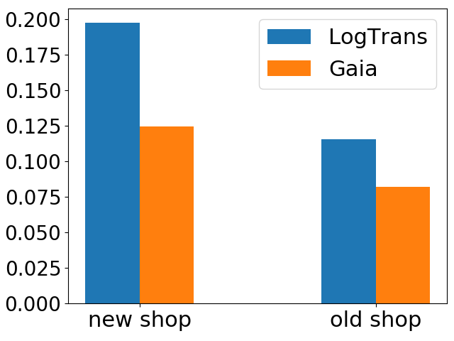
(a) MAPE

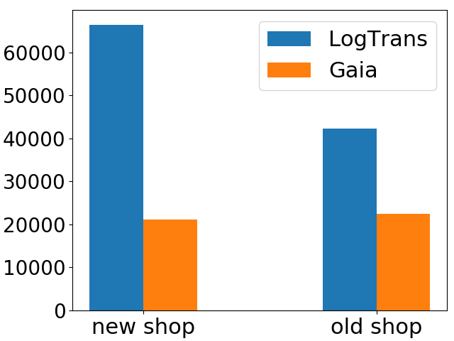
(b) MAE

Figure 3: Effectiveness Analysis of e-seller Graph. Larger performance margin between Gaia and LogTrans on the “New Shop Group” could be observed.

V-B4 Case Study towards the ITA module

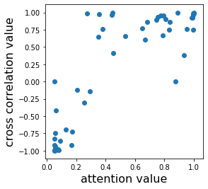
(a)

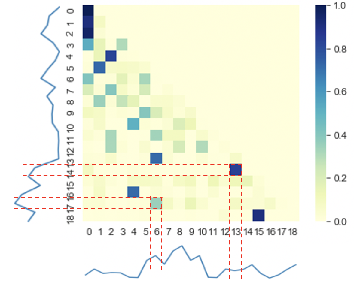
(b)

Figure 4: Case study of the ITA module. (a) Relationship between learned attention weights and cross correlation values for arbitrary GMV pairs in each individual GMV series, (b) Attention heatmap between a center node and one of its neighbors.

To better understand the merits of Gaia, we conduct a comprehensive case study for the ITA module, which intuitively provides convincing evidences for GMV forecasting with attentive weights. For intra temporal shift aware attention, we plot the relationship between the learned attention weights and correlation values for arbitrary GMV pairs in each individual GMV series. The negative correlation shown in Fig. 4 (a) concludes that similar temporal patterns in single GMV series could be well captured by Gaia. On the other hands, we present an attention heat map between a center node and one of its neighbors in Fig. 4 (b) to study the inter temporal shift aware attention. It is not surprising that similar patterns cross two nodes could be find with large attention. It is also worthwhile to note that a pair of unmatched temporal patterns also attains large attention due to the impact of auxiliary features.

VI System Deployment

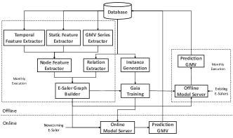
Figure 5: The deployment details of Gaia in simulated Alipay App environment.

To future demonstrate the effectiveness of the proposed Gaia, we deploy it in the Alipay’s simulated online environment for GMV forecasting. As shown in Fig. 5, our deployment follows a hybrid online-offline architecture: offline periodical training $\rightarrow$ online real-time prediction.

As mentioned above, a well-established e-seller graph is of crucial importance to support offline training. Assisted by the Node Feature Extractor and Relation Extractor, abundant features (i.e., temporal/static features and GMV series) and relations (i.e., same owner/shareholder and supply chain relationship) are fully explored in an automatic way. It is worthwhile to note that such a simulated pipeline is scheduled monthly to adapt our system to the ever-changing graph structure. In the online part, with regard to a newcoming e-seller, the well-trained Gaia stored in the Model Server will make prediction in real time based on its ego-subgraph extracted from the aforementioned e-seller graph.

Compared to the existed deployed baseline LogTrans, we observe that Gaia achieves 29.1% improvement on the main metric MAPE (0.117 $\rightarrow$ 0.083). Our deployed model takes about 10 minutes to predict 2 million e-sellers, the inference time scales linearly with the number of clients.

VII Conclusion

In this paper, we propose Gaia, a novel GMV forecasting framework for e-sellers, to address the temporal deficiency and temporal shift issue. Following the common hierarchical architecture, Gaia jointly models GMV series and auxiliary features in a fine-grained manner with Feature Fusion Layer (FFL), and then learns feature interaction along the timeline through Temporal Embedding Layer (TEL), followed by the well-designed Inter and intra Temporal shift aware Attention based Graph Neural Network (ITA-GCN). Extensive offline and online experiments show the effectiveness of Gaia.

References

- [1] Q. Yu, S. Yang, Z. Zhang, Y.-L. Zhang, B. Hu, Z. Liu, K. Huang, X. Zhong, J. Zhou, and Y. Fang, “A graph attention network model for gmv forecast on online shopping festival,” in Asia-Pacific Web (APWeb) and Web-Age Information Management (WAIM) Joint International Conference on Web and Big Data. Springer, 2021, pp. 134–139.
- [2] C. Chen, Z. Liu, J. Zhou, X. Li, Y. Qi, Y. Jiao, and X. Zhong, “How much can a retailer sell? sales forecasting on tmall,” in Pacific-Asia Conference on Knowledge Discovery and Data Mining. Springer, 2019, pp. 204–216.
- [3] G. E. Box, G. M. Jenkins, G. C. Reinsel, and G. M. Ljung, Time series analysis: forecasting and control. John Wiley & Sons, 2015.
- [4] S. Hochreiter and J. Schmidhuber, “Long short-term memory,” Neural computation, vol. 9, no. 8, pp. 1735–1780, 1997.
- [5] G. Lai, W.-C. Chang, Y. Yang, and H. Liu, “Modeling long-and short-term temporal patterns with deep neural networks,” in The 41st International ACM SIGIR Conference on Research & Development in Information Retrieval, 2018, pp. 95–104.
- [6] S. Yang, Z. Zhang, J. Zhou, Y. Wang, W. Sun, X. Zhong, Y. Fang, Q. Yu, and Y. Qi, “Financial risk analysis for smes with graph-based supply chain mining,” in IJCAI, 2020, pp. 4661–4667.
- [7] B. Yu, H. Yin, and Z. Zhu, “Spatio-temporal graph convolutional networks: A deep learning framework for traffic forecasting,” in IJCAI, 2018.
- [8] Z. Wu, S. Pan, G. Long, J. Jiang, and C. Zhang, “Graph wavenet for deep spatial-temporal graph modeling.” in IJCAI, 2019.
- [9] C. Zheng, X. Fan, C. Wang, and J. Qi, “Gman: A graph multi-attention network for traffic prediction,” in Proceedings of the AAAI Conference on Artificial Intelligence, vol. 34, no. 01, 2020, pp. 1234–1241.
- [10] S. Aminikhanghahi and D. J. Cook, “A survey of methods for time series change point detection,” Knowledge and information systems, vol. 51, no. 2, pp. 339–367, 2017.
- [11] R. Dürichen, M. A. Pimentel, L. Clifton, A. Schweikard, and D. A. Clifton, “Multitask gaussian processes for multivariate physiological time-series analysis,” IEEE Transactions on Biomedical Engineering, vol. 62, no. 1, pp. 314–322, 2014.
- [12] D. Salinas, V. Flunkert, J. Gasthaus, and T. Januschowski, “Deepar: Probabilistic forecasting with autoregressive recurrent networks,” International Journal of Forecasting, vol. 36, no. 3, pp. 1181–1191, 2020.
- [13] S. Li, X. Jin, Y. Xuan, X. Zhou, W. Chen, Y.-X. Wang, and X. Yan, “Enhancing the locality and breaking the memory bottleneck of transformer on time series forecasting,” Advances in Neural Information Processing Systems, vol. 32, pp. 5243–5253, 2019.
- [14] M. Maggiolo and G. Spanakis, “Autoregressive convolutional recurrent neural network for univariate and multivariate time series prediction,” arXiv preprint arXiv:1903.02540, 2019.
- [15] S.-Y. Shih, F.-K. Sun, and H.-y. Lee, “Temporal pattern attention for multivariate time series forecasting,” Machine Learning, vol. 108, no. 8, pp. 1421–1441, 2019.
- [16] Z. Wu, S. Pan, F. Chen, G. Long, C. Zhang, and S. Y. Philip, “A comprehensive survey on graph neural networks,” IEEE transactions on neural networks and learning systems, vol. 32, no. 1, pp. 4–24, 2020.
- [17] Z. Zhang, P. Cui, and W. Zhu, “Deep learning on graphs: A survey,” IEEE Transactions on Knowledge and Data Engineering, 2020.
- [18] P. Veličković, G. Cucurull, A. Casanova, A. Romero, P. Lio, and Y. Bengio, “Graph attention networks,” arXiv preprint arXiv:1710.10903, 2017.
- [19] W. L. Hamilton, R. Ying, and J. Leskovec, “Inductive representation learning on large graphs,” in Proceedings of the 31st International Conference on Neural Information Processing Systems, 2017, pp. 1025–1035.
- [20] T. N. Kipf and M. Welling, “Semi-supervised classification with graph convolutional networks,” arXiv preprint arXiv:1609.02907, 2016.
- [21] W. Chen, L. Chen, Y. Xie, W. Cao, Y. Gao, and X. Feng, “Multi-range attentive bicomponent graph convolutional network for traffic forecasting,” in Proceedings of the AAAI Conference on Artificial Intelligence, 2020, pp. 3529–3536.
- [22] S. Yan, Y. Xiong, and D. Lin, “Spatial temporal graph convolutional networks for skeleton-based action recognition,” in Thirty-second AAAI conference on artificial intelligence, 2018.
- [23] Y. Li, R. Yu, C. Shahabi, and Y. Liu, “Diffusion convolutional recurrent neural network: Data-driven traffic forecasting,” arXiv preprint arXiv:1707.01926, 2017.
- [24] Y. Seo, M. Defferrard, P. Vandergheynst, and X. Bresson, “Structured sequence modeling with graph convolutional recurrent networks,” in International Conference on Neural Information Processing, 2018, pp. 362–373.
- [25] Q. Xie, T. Guo, Y. Chen, Y. Xiao, X. Wang, and B. Y. Zhao, “Deep graph convolutional networks for incident-driven traffic speed prediction,” in Proceedings of the 29th ACM International Conference on Information & Knowledge Management, 2020, pp. 1665–1674.
- [26] Z. Wu, S. Pan, G. Long, J. Jiang, X. Chang, and C. Zhang, “Connecting the dots: Multivariate time series forecasting with graph neural networks,” in Proceedings of the 26th ACM SIGKDD International Conference on Knowledge Discovery & Data Mining, 2020, pp. 753–763.
- [27] F. Yu and V. Koltun, “Multi-scale context aggregation by dilated convolutions,” in 4th International Conference on Learning Representations, 2016.
- [28] G. Liu, Y. Mao, Q. Sun, H. Huang, W. Gao, X. Li, J. Shen, R. Li, and X. Wang, “Multi-scale two-way deep neural network for stock trend prediction.” in IJCAI, 2020, pp. 4555–4561.
- [29] A. Vaswani, N. Shazeer, N. Parmar, J. Uszkoreit, L. Jones, A. N. Gomez, Ł. Kaiser, and I. Polosukhin, “Attention is all you need,” in Advances in neural information processing systems, 2017, pp. 5998–6008.
- [30] S. Yang, B. Hu, Z. Zhang, W. Sun, Y. Wang, J. Zhou, H. Shan, Y. Cao, B. Ye, Y. Fang et al., “Inductive link prediction with interactive structure learning on attributed graph,” in Joint European Conference on Machine Learning and Knowledge Discovery in Databases. Springer, 2021, pp. 383–398.
- [31] C. Bergmeir, R. J. Hyndman, and B. Koo, “A note on the validity of cross-validation for evaluating autoregressive time series prediction,” Computational Statistics & Data Analysis, vol. 120, pp. 70–83, 2018.
- [32] P. Veličković, G. Cucurull, A. Casanova, A. Romero, P. Liò, and Y. Bengio, “Graph attention networks,” in International Conference on Learning Representations, 2018.
- [33] Z. Liu, C. Chen, L. Li, J. Zhou, X. Li, L. Song, and Y. Qi, “Geniepath: Graph neural networks with adaptive receptive paths,” in AAAI, vol. 33, 2019, pp. 4424–4431.
- [34] D. Zhang, X. Huang, Z. Liu, J. Zhou, Z. Hu, X. Song, Z. Ge, L. Wang, Z. Zhang, and Y. Qi, “Agl: a scalable system for industrial-purpose graph machine learning,” Proceedings of the VLDB Endowment, vol. 13, no. 12, pp. 3125–3137, 2020.
- [35] D. P. Kingma and J. Ba, “Adam: A method for stochastic optimization,” arXiv preprint arXiv:1412.6980, 2014.