$D=5$ static, charged black holes, strings and rings
with resonant, scalar $Q$-hair

Abstract:

A mechanism for circumventing the Mayo-Bekenstein no-hair theorem allows endowing four dimensional $(D=4)$ asymptotically flat, spherical, electro-vacuum black holes with a minimally coupled $U(1)$-gauged scalar field profile: $Q$-$hair$. The scalar field must be massive, self-interacting and obey a resonance condition at the threshold of (charged) superradiance. We establish generality for this mechanism by endowing three different types of static black objects with scalar hair, within a $D=5$ Einstein-Maxwell-gauged scalar field model: asymptotically flat black holes and black rings; and black strings which asymptote to a Kaluza-Klein vacuum. These $D=5$ $Q$-hairy black objects share many of the features of their $D=4$ counterparts. In particular, the scalar field is subject to a resonance condition and possesses a $Q$-ball type potential. For the static black ring, the charged scalar hair can balance it, yielding solutions that are singularity free on and outside the horizon.

1 Introduction

Influential results from the last three decades of the 20th century created a narrative that electrovacuum black holes (BHs) cannot support scalar “hair” [1] if: 1) the scalar model is physical, $i.e.$ it obeys appropriate energy conditions, and 2) only couples minimally to both the gravitational and electromagnetic fields - see [2] for a review. Two of the most influential theorems establishing the inexistence of scalar hair in these conditions, for uncharged and electrically charged BHs, respectively, were established by Bekenstein [4] and Mayo and Bekenstein [5].

In the last decade, however, this narrative was debunked. Firstly, it became clear that even for simple, physical, minimally coupled scalar models there is a generic mechanism allowing scalar hair around rotating (either neutral or electrically charged) BHs. This mechanism relies on a synchronization condition [6, 7]. Physically it means no scalar energy flux exists through the horizon, allowing equilbrium between the scalar environment and the trapped region. Mathematically, the scalar field circumvents one innocuous looking hypothesis (symmetry inheritance [8]) of the aforementioned Bekenstein theorem. This mechanism has proved to be quite universal, applying (say) to both neutral and electrically charged rotating BHs, with different asymptotics, dimensions and horizon topologies - see $e.g.$ [9, 10, 11, 12, 13, 14, 15, 16, 17], as well as to other spin fields [18, 19].

In some cases, the BHs with synchronized hair bifurcate from the bald solutions. This occurs when the latter admit a linear version of the BH hair, called stationary scalar clouds [20, 21, 22, 23], that exist at the threshold of the superradiant instability of spinning BHs [24]. This is the case for the paradigmatic Kerr solution of General Relativity; it means that creating synchronized hair is a natural dynamical process for Kerr BHs in the presence of such bosonic fields, as shown by numerical evolutions [25, 26] - see also the discussion in [27].

The situation for charged (non-spinning) BHs has both some some important similarities and some important differences as compared to that of spinning BHs. On the one hand, an analogous condition to the aforementioned synchronization condition – which in essence establishes the possibility of an equilibrium between the hair and the horizon – is possible for charged BHs; in this context it is called resonance condition. Explicitly, it means that

$$w=g_{s}V\big{|}_{{\cal H}},$$ (1.1)

where $w$ is the scalar field frequency, $g_{s}$ is the gauge coupling constant and $V\big{|}_{{\cal H}}$ is the value of the electric gauge potential at the horizon. One the other hand, albeit a version of superradiance (charged superradiance [24]) occurs for charged BHs, there are no scalar stationary clouds around the paradigmatic Reissner-Nordström (RN) BHs, at the threshold of charged superradiance [28, 29], except some marginally bound states at extremality [30], for a massive gauged scalar field model. This provides an impediment for hairy BHs bifurcating from the RN solution, akin to those birfurcation from the Kerr solution, thus vindicating the Mayo-Bekenstein theorem.

In an interesting development, however, it was shown in [31, 32, 33] that static hairy BH solutions in Einstein-Maxwell-gauged scalar field (EMgS) theory do exist, but only if the scalar field possesses both a mass term plus self-interactions; the latter invalidate one hypothesis of the Mayo-Bekenstein theorem. Additionally, the no go result in Ref. [29] is also circumvented, since the scalar field does not become infinitesimally small ($i.e.$ the non-linearities are always relevant). That is, the solutions in [31, 32, 33] are not zero modes of the superradiant instability and instead can be viewd as non-linear gauged Q-clouds, in the spirit of (test field) $Q$-ball like solitons around BHs, first considered in [34].

The main purpose of this work is to address the generality of the mechanism unveiled in [31, 32, 33] for endowing static, charged BHs with resonant, scalar $Q$-hair. To do so, we are gone consider the arena of higher dimensional BHs, which is more generous in terms of the possible black objects, even in vacuum and electrovacuum [35]. In four spacetime dimensions $(D=4)$ for asymptotically flat BH solutions only a spherical horizon topology is allowed. But as the dimension increases, the phase structure of the possible General Relativity (GR) black objects becomes increasingly intricate and diverse [35]. In this work we shall consider three different types of static $D=5$ solutions, corresponding to BHs, Black Rings (BRs) and Black Strings (BSs). The BHs and BRs approach asymptotically a five dimensional Minkowski spacetime background being distinguished by their different horizon topology, while the BSs are solutions in a Kaluza-Klein (KK) theory. This allows us to attempt the construction of different types of BHs with resonant, gauged, $Q$-hair.

We shall focus on a complex massive scalar field with ($Q$-ball type) quartic plus hexic self-interactions and establish that all qualitative results found in [31, 32, 33] hold also for the aforementioned $D=5$ black objects. Remarkably, in all cases studied, the emerging picture displays common patterns. A crucial ingredient for the existence of such regular black objects is the resonance condition (1.1). Moreover, this result is independent on the self-gravity effects: Maxwell-gauged scalar (MgS) solutions exist already in the probe limit ($i.e.$ for a vacuuum black object background). In all cases, the coupling with gravity leads to a maximal horizon size (which depends on the input parameters of the problem), with a multi-branch structure of the space of solutions. Moreover, owing to the pattern similarities for the $D=4$ and $D=5$ cases, we can reasonably expect that similar BHs with gauged scalar hair exist for any $D>5$.

This paper is organised as follows. In Section 2 we present the EMgS models and propose a classification of the solutions, based on their asymptotic behaviour. The scaling symmetries and the generic features of the solutions are also discussed. Section 3 deals with solutions found by solving a set of ordinary differential equations (ODEs) – the BHs and BSs. In Section 4, we study the BRs and provide numerical evidence for the existence of balanced configurations, free of singularities on and outside the horizon. We conclude in Section 5 with a discussion and some further remarks. The Appendix contains a brief review of three exact (static) solutions in (pure) Einstein-Maxwell theory, corresponding to the $D=5$ RN BH, charged BR and charged BS.

2 The general framework

2.1 The action and field equations

Working in $D=5$ spacetime dimensions, we consider the EMgS action:

$$\mathcal{S}=\int d^{5}x\sqrt{-g}\left(\frac{R}{16\pi G}-\frac{1}{4}F_{ab}F^{ab}-D_{a}\Psi^{*}D^{a}\Psi-U(\left|\Psi\right|)\right)~{},$$ (2.1)

where $G$ is the gravitational constant, $R$ is the Ricci scalar associated with the spacetime metric $g_{ab}$, $F_{ab}=\partial_{a}A_{b}-\partial_{b}A_{a}$ is the $U(1)$ field strength tensor, and

$$D_{a}\Psi=\partial_{a}\Psi+ig_{s}A_{a}\Psi\ ,$$ (2.2)

is the gauge covariant derivative, with $g_{s}$ the gauge coupling constant. $U(|\Psi|)>0$ denotes the potential of the complex scalar field $\Psi$, whose mass $\mu$ is defined by

$$\mu^{2}\equiv\frac{\partial U}{\partial|\Psi|^{2}}\bigg{|}_{\Psi=0}\ .$$ (2.3)

The EMgS field equations, obtained by varying the action with respect to the metric, scalar field and electromagnetic field, are, respectively,

$$R_{ab}-\frac{1}{2}g_{ab}R=8\pi G\left(T_{ab}^{\rm(M)}+T_{ab}^{(\Psi)}\right),$$ (2.4)

$$D_{a}D^{a}\Psi=\frac{\partial U}{\partial\left|\Psi\right|^{2}}\Psi\ ,\qquad\nabla_{a}F^{ba}=ig_{s}\big{[}\Psi^{*}(D^{b}\Psi)-(D^{b}\Psi^{*})\Psi)\big{]}~{}\equiv g_{s}j^{b}~{},$$ (2.5)

with two different components in the total energy-momentum tensor

$$T_{ab}^{\rm(M)} = F_{a}^{~{}c}F_{bc}-\frac{1}{4}g_{ab}F_{cd}F^{cd},~{}$$ (2.6)

$$T_{ab}^{(\Psi)} = D_{a}\Psi^{*}D_{b}\Psi+D_{b}\Psi^{*}D_{a}\Psi-g_{ab}\left[\frac{1}{2}g^{cd}(D_{c}\Psi^{*}D_{d}\Psi+D_{d}\Psi^{*}D_{c}\Psi)+U(\left|\Psi\right|)\right]\ .$$

This model is invariant under the local $U(1)$ gauge transformation

$$\psi\to\psi e^{-ig_{s}\alpha}\ ,\qquad A_{\mu}\to A_{\mu}+\partial_{\mu}\alpha\ ,$$ (2.7)

with $\alpha$ a real function of $x^{a}$. Also, $j^{a}$ is the conserved current, $\nabla_{a}j^{a}=0$.

2.2 Classes of solutions and global charges

All geometries discussed in this work are static, with a generic line element (see (3.1), (3.6), (4.1)):

$$ds^{2}=g_{tt}(\vec{x})dt^{2}+g_{ij}(\vec{x})dx^{i}dx^{j}\ ,$$ (2.8)

where $x^{a}=(t,\vec{x})$ and $t$ is the time coordinate. The matter fields are of the form

$$\Psi(\vec{x},t)=\psi(\vec{x})e^{-iwt}\ ,\qquad A(\vec{x},t)=V(\vec{x})dt\ ,$$ (2.9)

with $\psi$ and $V$ real functions and $w$ the scalar field frequency.

There is also a discrete symmetry

$$V\to-V,~{}~{}g_{s}\to-g_{s},$$ (2.10)

which allows us to consider the case $g_{s}\geq 0$ only.

Within this framework, the only nonvanishing component of the conserved current is

$$j^{t}={2(w-g_{s}V)\psi^{2}}g^{tt},$$ (2.11)

the associated Noether charge (particle number) being

$$Q_{N}=\int d^{4}x\sqrt{-g}j^{t},$$ (2.12)

with the integral evaluated in the region outside the horizon. In the generic case, the Noether charge provides a part of the total electric charge (as computed from the flux of the electric field at infinity), which, from the second equation in (2.5), can be written as the sum (with $Q_{H}$ the horizon charge)

$$Q_{e}=Q_{H}+g_{s}Q_{N}\ ,\qquad{\rm where}~{}~{}Q_{H}=\oint_{{\cal H}}dS_{i}F^{ti}~{}.$$ (2.13)

2.2.1 A Minkowski spacetime background

Two classes of solutions discussed in this work, the BHs and the BR – $cf.$ eqs. (3.1) and (4.1) below, respectively –, approach asymptotically a five dimensional Minkowski spacetime background $\mathbb{M}^{1,4}$, with a line element

$$ds^{2}=-dt^{2}+dr^{2}+r^{2}d\Omega_{3}^{2}\ ,\qquad{\rm with}\qquad d\Omega_{3}^{2}=d\theta^{2}+\cos^{2}\theta d\varphi_{1}^{2}+\sin^{2}\theta d\varphi_{2}^{2}\ ,$$ (2.14)

where the range of $\theta$ is $0\leq\theta\leq\pi/2$ and with $0\leq(\varphi_{1},\varphi_{2})\leq 2\pi$. Also, $r$ and $t$ correspond to the radial and time coordinates, respectively. The solutions possess a nonzero mass $M$ and an electric charge $Q_{e}$, which are read off from the far field asymptotics of the metric function $g_{tt}$ and of the electric potential $V$, respectively,

$$g_{tt}=-1+\frac{8GM}{3\pi r^{2}}+\dots\ ,\qquad V=\Phi-\frac{Q_{e}}{4\pi^{2}r^{2}}+\dots\ ,$$ (2.15)

with $\Phi$ the chemical potential (for the gauge discussed below). The solutions possess an horizon which can be of spherical topology, $S^{3}$ (BHs) or of $S^{2}\times S^{1}$ topology (BRs). The event horizon has a nonvanishing area $A_{H}$. The Hawking temperature $T_{H}$ of all of the considered solutions is also nonzero, and can be computed from their surface gravity.

In order to compare the pattern of the hairy solutions with that of the known electrovacuum BHs, it is useful to consider reduced quantities, with horizon area, Hawking temperature and electric charge normalized $w.r.t.$ the mass of the solutions

$$a_{H}=\frac{3}{32}\sqrt{\frac{3}{2\pi}}\frac{A_{H}}{(GM)^{3/2}}\ ,\qquad t_{H}=4\sqrt{\frac{2\pi}{3}}T_{H}\sqrt{GM}\ ,\qquad q=\frac{\sqrt{3G}}{4\sqrt{\pi}}\frac{Q_{e}}{GM}~{},$$ (2.16)

with the coefficients chosen such that $a_{H}=t_{H}=1$ in the Schwarzschild-Tangerlini limit, while $q=1$ for an extremal ($D=5$) RN background – see Appendix A.

For any horizon topology, the solutions satisfy the 1st law of thermodynamics

$$dM=\frac{T_{H}}{4G}dA_{H}+\Phi dQ_{e}\ ,$$ (2.17)

and the Smarr relation:

$$M=\frac{3}{2}T_{H}\frac{A_{H}}{4G}+\Phi Q_{e}+M_{(\psi)},$$ (2.18)

with $M_{(\psi)}$ the mass outside the horizon stored in the scalar field, which, for the chosen gauge (see the discussion in Section 2.4) takes the simple form

$$M_{(\psi)}=\int d^{4}x\sqrt{-g}\left(\frac{1}{2}g_{s}Vj^{t}-U(\psi)\right)\ ,$$ (2.19)

with the integral evaluated in the region outside the horizon.

2.2.2 A Kaluza-Klein spacetime background

The second case corresponds to black objects approaching asymptotically four dimensional Minkowski spacetime times a circle, $\mathbb{M}^{1,3}\times S^{1}$. We denote the compact direction as $z$, with an arbitrary periodicity $L$, such that the background spacetime metric is

$$ds^{2}=-dt^{2}+dr^{2}+r^{2}d\Omega_{2}^{2}+dz^{2},$$ (2.20)

with $d\Omega_{2}^{2}$ the metric on a two-sphere.

For any static spacetime which is asymptotically $\mathbb{M}^{1,3}\times S^{1}$ one can define a mass $M$, a tension ${\cal T}$, and an electric charge $Q_{e}$, these quantities being encoded in the asymptotics of the metric potentials [39, 40] and of the electrostatic potential, with

$$g_{tt}=-1+\frac{c_{t}}{r}+\dots\ ,\qquad g_{zz}=1+\frac{c_{z}}{r}+\dots\ ,\qquad V=\Phi-\frac{1}{4\pi L}\frac{Q_{e}}{r}+\dots\ ,$$ (2.21)

and

$$M=\frac{L}{4G}(2c_{t}-c_{z})\ ,\qquad{\cal T}=\frac{1}{4G}(c_{t}-2c_{z})\ .$$ (2.22)

One can also define a relative tension $n={{\cal T}L}/{M},$ with $n=1/2$ for a Schwarzschild BS, while $0\leq n\leq 1/2$ for a BS in Einstein-Maxwell (EM) theory. The BSs possess also an horizon area $A_{H}$ and a Hawking temperature $T_{H}$. As with the solutions with $\mathbb{M}^{1,4}$ asymptotics, we define a set of reduced quantities normalized $w.r.t.$ mass,

$$a_{H}=\frac{1}{16\pi}\frac{A_{H}L}{(GM)^{2}},\qquad t_{H}=8\pi T_{H}\frac{GM}{L},\qquad q=\frac{3\sqrt{G}}{4\sqrt{3\pi}}\frac{Q_{e}L}{GM}~{},$$ (2.23)

such that $a_{H}=t_{H}=1$ is the Schwarzschild-BS limit, while $q=1$ for an extremal BS solution in EM theory (see the discussion in Appendix A).

For Kaluza-Klein asymptotics, the 1st law of thermodynamics contains an extra-term,

$$dM=\frac{T_{H}}{4G}dA_{H}+\Phi dQ_{e}+{\cal T}dL,$$ (2.24)

and so does the Smarr relation,

$$M=\frac{3}{2}\frac{T_{H}}{4G}A_{H}+\Phi Q_{e}+\frac{1}{2}{\cal T}L+M_{(\psi)},$$ (2.25)

with $M_{(\psi)}$ still given by (2.19).

2.3 The potential and scaling properties

For a quantitative study of the solutions, we need to specify the expression of the potential $U(\left|\Psi\right|)$. Following the previous $D=4$ work, the results in this paper are for a potential which is the sum of a mass term plus quartic and sextic self-interactions:

$$U(|\Psi|)=\mu^{2}|\Psi|^{2}-\lambda|\Psi|^{4}+\nu|\Psi|^{6}~{},$$ (2.26)

where $\mu$ is the scalar field mass and $\lambda,\nu$ are positive parameters (with $\lambda^{2}<4\mu^{2}\nu$ for a strictly positive potential, $U(|\Psi|)>0)$. As with the $D=4$ case, the presence of higher order terms in the scalar potential appears to be mandatory, and we have failed to find hairy solutions for a scalar field with a mass term only.

In the numerics, it is useful to work with a set of scaled, dimensionless: $i)$ model input parameters; $ii)$ matter functions; and $iii)$ a dimensionless radial coordinate. These are defined as (denoted with overbar in what follows):

$$w=\bar{w}\mu,\qquad g_{s}=\bar{g}_{s}\sqrt{\lambda},\qquad V=\bar{V}\frac{\mu}{\sqrt{\lambda}},\qquad\Psi=\bar{\Psi}\frac{\mu}{\sqrt{\lambda}}\qquad{\rm and}\qquad r=\frac{\bar{r}}{\mu}.$$ (2.27)

This scaling reveals the existence of three input dimensionless parameters

$$\alpha^{2}=\frac{4\pi G\mu^{2}}{\lambda},\qquad\beta^{2}=\frac{\nu\mu^{2}}{\lambda},\qquad\bar{g}_{s}=g_{s}\sqrt{\lambda}\mbox{e}e~{},$$ (2.28)

which characterize a given model.

Under the transformation (2.27), several quantities of interest behave as

$$M=\frac{\bar{M}}{\mu^{2}G},\qquad Q_{e}=\frac{\bar{Q}_{e}}{\mu\sqrt{\lambda}},\qquad\Phi=\bar{\Phi}\frac{\mu}{\sqrt{\lambda}}\qquad A_{H}=\frac{\bar{A}_{H}}{\mu^{3}},\qquad T_{H}=\bar{T}_{H}\mu\ .$$ (2.29)

The numerics is done with the scaled quantities and functions, and dimensionless parameters. With these conventions, the Einstein equations solved numerically are $R_{\mu\nu}-\frac{1}{2}g_{\mu\nu}{R}=2\alpha^{2}~{}T_{\mu\nu}$, while the scaled scalar potential – for the ansatz (2.9) – is $U(\bar{\psi})=\bar{\psi}^{2}-\bar{\psi}^{4}+\beta^{2}\bar{\psi}^{6}.$ However, to simplify the picture, we shall ignore the overbar in the plots for $V$ and $\psi$. Also, for the sake of clarity all equations displayed in what follows are given in terms of dimensionful variables.

2.4 The bound state condition and fixing the gauge

For large-$r$, the deviation from the background geometry can be neglected to leading order in the scalar field equation. This leads to the following asymptotic expression of the scalar field

$$\psi(r)\sim\frac{e^{-\mu_{\rm eff}r}}{r^{3/2}}+\dots,~{}~{}{\rm for~{}BHs~{}and~{}BRs},~{}~{}{\rm and}~{}~{}\psi(r)\sim\frac{e^{-\mu_{\rm eff}r}}{r}+\dots,~{}~{}{\rm for~{}BSs},$$ (2.30)

where we define

$$\mu_{\rm eff}=\sqrt{\mu^{2}-(w-g_{s}\Phi)^{2}}.$$ (2.31)

A simple inspection of the equations reveals that the scalar field frequency $w$ enters always in the combination $w-g_{s}V$. Thus the model still possesses the residual gauge symmetry

$$w\to w+\gamma,\qquad V\to V+s\gamma/g_{s}~{},$$ (2.32)

(with $\gamma$ a real number) which should be fixed in numerics. Following [32], we work in a gauge with a vanishing electric potential at the horizon,

$$V\big{|}_{{\cal H}}=0.$$ (2.33)

Then the regularity condition (1.1) implies $w=0$, $i.e.$ a real scalar field. As such, the matter Lagrangian of the model can be written in the suggestive form

$$\mathcal{L}_{m}=-\frac{1}{4}F_{ab}F^{ab}-\partial_{a}\psi\partial^{a}\psi-g_{s}^{2}A_{a}A^{a}\psi^{2}-U(\psi),$$ (2.34)

with the vector potential acquiring a local mass. Note, however, that $\psi$ is not a Higgs field, since it vanishes asymptotically.

It is also interesting to investigate the status of the Mayo-Bekenstein no-go result [5] for the considered $D=5$ configurations. The starting point is the equation for the electric potential $V$, which, in the chosen gauge is

$$\nabla_{a}F^{ta}=-2g^{tt}g_{s}\psi^{2}V~{}.$$ (2.35)

Multiplying it by $V$ and integrating by parts yields

$$\oint_{\infty}dS_{i}VF^{ti}=\Phi Q_{e}=-\int d^{4}x\sqrt{-g}g^{tt}\left[g^{ab}\partial_{a}V\partial_{b}V+2g_{s}V^{2}\psi^{2}\right],$$ (2.36)

where we have used condition (2.33). Since the $r.h.s.$ of the above expression is strictly positive, this implies that the solutions necessarily have nonzero $Q_{e}$ and $\Phi$. If, as assumed by Mayo and Bekenstein, there is no mass term in the potential $U(\psi)$ (or $\mu<g_{s}\Phi$) the scalar field would possess wave-like asymptotics (see the eq. (2.30)), and thus one is forced to impose $\Phi=0$. Then (2.36) implies that the scalar field necessarily vanishes.

2.5 Generic features of the solutions

In Sections 3 and 4, we shall present the equations and the boundary conditions, together with a study of the solutions for the different hairy black objects we shall construct. Without entering into details, here we summarize their common basic features.

• Within the considered framework, the numerical problem contains five input parameters

  $$\{\alpha,\beta,e;\Phi;r_{H}\};$$ (2.37)

  the first three correspond to constants of the model, while $\Phi$ is the asymptotic value of the electric potential and $r_{H}$ is the horizon radius. For the BRs, there is one more input parameter, the ring’s radius $R$. The construction reduces to solving a set of ODEs (for BHs and BSs) or Partial Differential Equations (for BRs). The quantities of interest are computed from the numerical output.

• The limit of a vanishing scalar field $\psi=0$ is a consistent solution of the model. In this case we recover the known (static) BHs, BRs and BSs in EM theory, whose basic properties are reviewed in Appendix A.

• Apart from the EM solutions, there are black objects with gauged scalar hair. However, the scalar field does not emerge as a zero mode of an electrovacuum solution. That is, the scalar field never trivializes, with the necessary existence of non-linear terms in the scalar potential.

• The solutions satisfy the resonance condition (1.1), which emerges from assuming the existence of a power series expansion of the solutions close to the horizon together with regularity conditions. Also, working in a gauge with $w=0$, the solutions satisfy the bound state condition

  $$g_{s}\Phi\leq\mu.$$ (2.38)

• Non-linear gauged $Q$-clouds exist already in the decoupling limit of the model, $i.e.$ when ignoring the backreaction of the scalar and Maxwell field on the geometry and solving MgS field equations on a fixed background which corresponds to the Schwarzschild-Tangherlini BH, a vacuum BR and a Schwarzschild BS, respectively.

• The solutions of the full EMgS model display a complicated pattern, with a maximal horizon size and different branches of solutions. The branch of fundamental solutions possesses a well defined horizonless limit corresponding to charged $Q$-balls (for a $\mathbb{M}^{1,4}$ background) and $Q$-vortices (in the $\mathbb{M}^{1,3}\times S^{1}$ case).

• All reported solutions have a non-zero Hawking temperature, while the model is unlikely to possess extremal BH solutions.

3 Co-dimension one solutions. Black Holes and Black Strings

The BHs and BSs discussed in this work solve a set of ODEs with suitable boundary conditions. Since the treatment of the numerical problem together with the unveiled picture is rather similar, we report them together in what follows.

3.1 The Ansatz and equations

3.1.1 Black holes

In the numerical study of the spherically symmetric solutions, it is convenient to use the following metric Ansatz:

$$ds^{2}=-N(r)\sigma^{2}(r)dt^{2}+\frac{dr^{2}}{N(r)}+r^{2}d\Omega_{3}^{2}\ ,$$ (3.1)

while the matter functions $\psi$ and $V$ depend on the radial coordinate $r$ only. Then the corresponding field equations, as resulting from (2.4), (2.5) read

$$N^{\prime}+\frac{2}{r}(N-1)+\frac{16\pi G}{3}r\left[\frac{V^{\prime 2}}{2\sigma^{2}}+N\psi^{\prime 2}+U(\psi)+\frac{(w-g_{s}V)^{2}}{N\sigma^{2}}\psi^{2}\right]=0,$$

$$\sigma^{\prime}=\frac{16\pi G}{3}r\sigma\left[\psi^{\prime 2}+\frac{(w-g_{s}V)^{2}\psi^{2}}{N^{2}\sigma^{2}}\right],$$ (3.2)

$$V^{\prime\prime}+\left(\frac{3}{r}-\frac{\sigma^{\prime}}{\sigma}\right)V^{\prime}+\frac{2q_{s}(w-g_{s}V)\psi^{2}}{N}=0,$$

$$\psi^{\prime\prime}+\left(\frac{3}{r}+\frac{N^{\prime}}{N}+\frac{\sigma^{\prime}}{\sigma}\right)\psi^{\prime}+\frac{(w-g_{s}V)^{2}\psi}{N^{2}\sigma^{2}}-\frac{1}{2N}\frac{dU}{d\psi}=0~{}.$$

The non-vanishing components of the energy-momentum tensor are

$$T_{r}^{r(M)}=-\frac{V^{\prime 2}}{2\sigma^{2}},\qquad T_{r}^{r(\Psi)}=N\psi^{\prime 2}+\frac{(w-g_{s}V)^{2}\psi^{2}}{N\sigma^{2}}-U(\psi)\ ,$$

$$T_{\Omega}^{\Omega(M)}=\frac{V^{\prime 2}}{2\sigma^{2}}\ ,\qquad T_{\Omega}^{\Omega(\Psi)}=-N\psi^{\prime 2}+\frac{(w-g_{s}V)^{2}\psi^{2}}{N\sigma^{2}}-U(\psi),$$ (3.3)

$$T_{t}^{t(M)}=-\frac{V^{\prime 2}}{2\sigma^{2}}\ ,\qquad T_{t}^{t(\Psi)}=-N\psi^{\prime 2}-\frac{(w-g_{s}V)^{2}\psi^{2}}{N\sigma^{2}}-U(\psi)~{},$$

with $\Omega=(\theta,\varphi_{1},\varphi_{2})$. The horizon is located at $r=r_{H}>0$ with $N(r)\sim(r-r_{H})$ as $r\to r_{H}$, while the metric function $\sigma(r)$ remains nonzero (and finite) in the same limit. The Hawking temperature and the event horizon area of the solutions are found from the horizon data,

$$T_{H}=\frac{1}{4\pi}N^{\prime}(r_{H})\sigma(r_{H})\ ,\qquad A_{H}=2\pi^{2}r_{H}^{3}~{}.$$ (3.4)

We assume the existence of a power series of the solutions in $(r-r_{H})$ close to the horizon. Then the finiteness of the energy-momentum tensor (3.3) (or of the current density (2.11)) implies the following condition

$$\psi(r_{H})(w-g_{s}V(r_{H}))=0\ ,$$ (3.5)

which can be satisfied by taking (1.1) or by taking $\psi(r_{H})=0$. However, the latter choice implies that the derivatives of the scalar field vanish order by order in the power series expansion close to the horizon; that is, the scalar field trivializes. Thus the only reasonable solution is the resonance condition (1.1).

3.1.2 Black strings

The line element in this case contains three unknown functions, with

$$ds^{2}=-b(r)dt^{2}+\frac{dr^{2}}{f(r)}+r^{2}d\Omega_{2}^{2}+a(r)dz^{2},$$ (3.6)

with $\psi$ and $V$ functions of $r$ only. Then the EMgS equations read

$$f^{\prime}+\frac{2(f-1)}{r}+\bigg{(}\frac{a^{\prime}}{a}+\frac{b^{\prime}}{b}\bigg{)}f+\frac{32\pi G}{3}r\left[\frac{f}{2b}V^{\prime 2}+U(\psi)\right]=0\ ,$$

$$a^{\prime}\bigg{(}b+\frac{1}{4}rb^{\prime}\bigg{)}+\bigg{[}b^{\prime}+\frac{b}{r}\bigg{(}1-\frac{1}{f}\bigg{)}\bigg{]}a+8\pi Gra\left[\frac{1}{2}V^{\prime 2}-b\psi^{\prime 2}+\frac{b}{f}U(\psi)-\frac{(w-g_{s}V)^{2}}{f}\psi^{2}\right]=0\ ,$$

$$b^{\prime\prime}+\left[\frac{1}{r}\bigg{(}1+\frac{1}{f}\bigg{)}-\frac{b^{\prime}}{b}\right]b^{\prime}+\frac{16\pi G}{3}\left[-\frac{6(w-g_{s}V)^{2}}{f}\psi^{2}-2(1+\frac{rb^{\prime}}{4b})V^{\prime 2}+\frac{2b-rb^{\prime}}{f}U(\psi)\right]=0\ ,$$

$$\psi^{\prime\prime}+\frac{1}{2}\left(\frac{4}{r}+\frac{a^{\prime}}{a}+\frac{b^{\prime}}{b}+\frac{f^{\prime}}{f}\right)\psi^{\prime}+\frac{(w-g_{s}V)^{2}}{bf}\psi-\frac{1}{2}\frac{dU}{d\psi}\frac{\psi}{f}=0\ ,$$ (3.7)

$$V^{\prime\prime}+\frac{1}{2}\left(\frac{4}{r}+\frac{a^{\prime}}{a}+\frac{b^{\prime}}{b}+\frac{f^{\prime}}{f}\right)V^{\prime}+\frac{2g_{s}(w-g_{s}V)\psi^{2}}{f}=0~{}.$$

The non-vanishing components of the energy-momentum tensor are

$$T_{r}^{r(M)}=-\frac{fV^{\prime 2}}{2b}\ ,\qquad T_{r}^{r(\Psi)}=f\psi^{\prime 2}+\frac{(w-g_{s}V)^{2}\psi^{2}}{b}-U(\psi)\ ,~{}~{}$$

$$T_{\Omega}^{\Omega(M)}=\frac{fV^{\prime 2}}{2b}\ ,\qquad T_{\Omega}^{\Omega(\Psi)}=-f\psi^{\prime 2}+\frac{(w-g_{s}V)^{2}\psi^{2}}{b}-U(\psi)\ ,~{}~{}$$

$$T_{t}^{t(M)}=-\frac{fV^{\prime 2}}{2b}\ ,\qquad T_{t}^{t(\Psi)}=-f\psi^{\prime 2}-\frac{(w-g_{s}V)^{2}\psi^{2}}{b}-U(\psi)~{},$$ (3.8)

$$T_{z}^{z(M)}=\frac{fV^{\prime 2}}{2b}\ ,\qquad T_{z}^{z(\Psi)}=-f\psi^{\prime 2}+\frac{(w-g_{s}V)^{2}\psi^{2}}{b}-U(\psi)~{}.$$

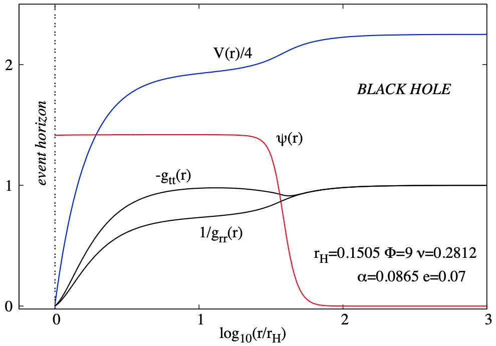
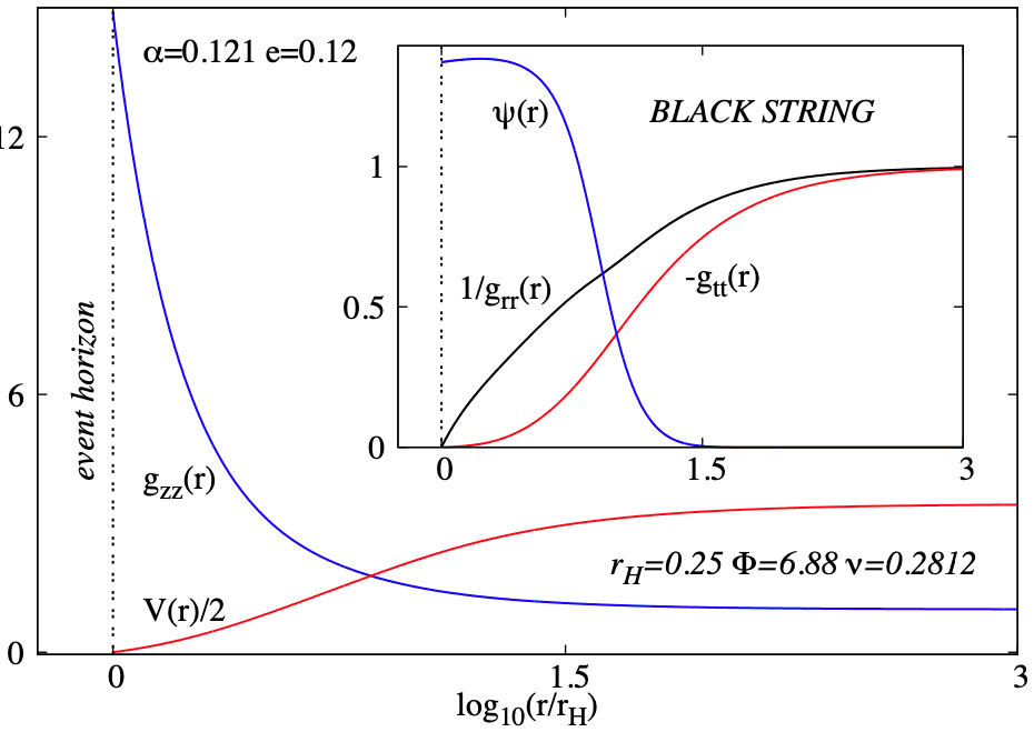
Figure 1: Profile functions of a typical BH (left) and BS (right) are shown as functions of the radial coordinate.

The horizon is again located for some $r=r_{H}>0$, where $f(r_{H})=b(r_{H})=0$, while $a(r_{H})>0$. The horizon area and Hawking temperature are

$$A_{H}=4\pi r_{H}^{2}L\sqrt{a(r_{H})}\ ,\qquad T_{H}=\frac{1}{4\pi}\sqrt{f^{\prime}(r_{H})b^{\prime}(r_{H})}~{}.$$ (3.9)

As with the BHs, the resonance condition (1.1) necessarily emerges when assuming the existence of a power series expansion of the solutions close to the horizon.

3.2 The results

In the absence of closed form solutions, the set of four (five) ODEs (3.2) (and (3.7), respectively) are solved numerically, by using a professional solver that employs a collocation method for boundary value ODEs equipped with an adaptive mesh selection procedure [41]. Typical mesh sizes include few hundred points, the relative accuracy of the solutions being around $10^{-10}$. The boundary conditions we have imposed are:

$${\bf BHs}:~{}N\big{|}_{r=r_{H}}=V\big{|}_{r=r_{H}}=\psi\big{|}_{r=\infty}=0,~{}\bigg{[}N^{\prime}\psi^{\prime}-\frac{1}{2}\frac{dU}{d\psi}\bigg{]}_{r=r_{H}}=0,~{}N\big{|}_{r=\infty}=1,~{}V\big{|}_{r=\infty}=\Phi,~{}$$

$${\bf BSs}:~{}f|_{r=r_{H}}=b|_{r=r_{H}}=V|_{r=r_{H}}=0,~{}~{}\bigg{[}\bigg{(}\frac{a^{\prime}}{a}+\frac{b^{\prime}}{b}\bigg{)}\psi^{\prime}-\frac{1}{2}\frac{dU}{d\psi}\bigg{]}_{r=r_{H}}=0,~{}~{}$$ (3.10)

$${~{}~{}~{}~{}~{}~{}~{}~{}~{}}f\big{|}_{r=\infty}=b\big{|}_{r=\infty}=1,~{}~{}V\big{|}_{r=\infty}=\Phi,~{}~{}\psi\big{|}_{r=\infty}=0,~{}~{}a\big{|}_{r=\infty}=1,~{}~{}$$

which result from a study of the near horizon and far field approximate form of the solutions.

The profiles of a typical BH/BS solution is shown in Figure 1. One can see that in both cases the matter functions monotonically interpolate between the horizon and infinity. Solutions with nodes for both $V$ and $\psi$ do also exist; in particular, we have found numerical evidence for the existence of $D=5$ generalizations of the four-dimensional ’wavy’ hairy BH discussed in [42, 43]. However, in this work we shall restrict ourselves to the study of nodeless configurations.

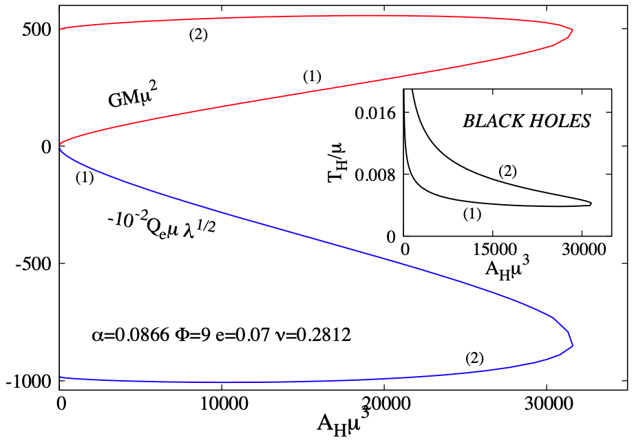
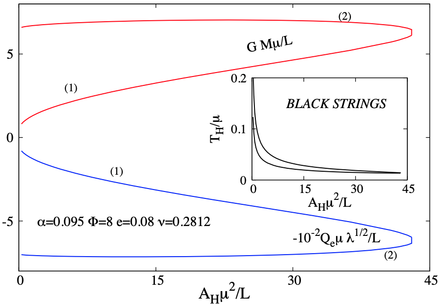
Figure 2: The mass, electric charge and Hawking temperature of solutions are shown as a function of event horizon area for BHs and BSs. The quantities are shown in the natural units of the model.

The complete classification of the solutions in the space of physical parameters $(\alpha,\beta,e)$ is a considerable task which is not the goal of this work. Here, for both BHs and BSs (and also for BRs in the next Section) we shall present illustrative results for a selected set $(\alpha,\beta,e)$ in each case, as a proof of concept. Also, the BH/BS horizon size is varied for a fixed value of the electrostatic potential $\Phi$ – that is, we study solutions in a grand canonical ensemble –, and we do not consider the case with a fixed electric charge.

When reporting on the properties of the solutions, it is natural to start with their horizonless limit, approached as $r_{H}\to 0$. This nontrivial limit exists due to the scalar field interaction, being absent (or pathological) for the pure Einstein-Maxwell case. It corresponds to gauged $Q$-balls (for a $\mathbb{M}^{1,4}$ background) and gauged $Q$-vortices (for a $\mathbb{M}^{1,3}\times S^{1}$ background). These are $D=5$ natural counterparts of the four dimensional EMgS solitonic solutions reported in [44, 45, 46, 47, 48], and appear to share with them all basic properties. In particular, when fixing the input parameters of the model $(\alpha,\beta,e)$, the horizonless solutions exist again for a finite range of the parameter $\Phi$, the upper limit being fixed by the bound state condition (2.38), while $\Phi_{\rm min}$ is nonzero and results from numerics.

Any gauged $Q$-ball/$Q$-vortex solution appears to possess BH generalizations. Given the parameter $(\alpha,\beta,e;\Phi)$, the BHs and BSs are found by slowly increasing from zero the value of event horizon radius. As shown in Figures 2, 3, the solutions with a fixed chemical potential $\Phi$ exist up to a maximal BH size, as specified by the event horizon area $A_{H}$.

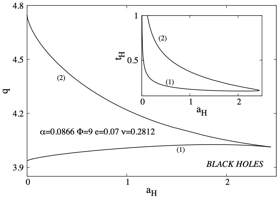
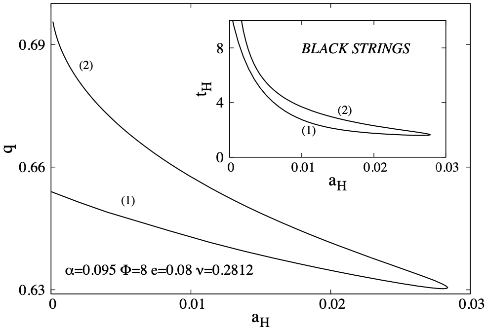
Figure 3: The reduced electric charge and Hawking temperature are shown as a function of reduced horizon area for BHs and BSs. The quantities are shown in units set by the mass of the solutions.

Along this fundamental branch (denoted with (1) in the plots), both the mass and the electric charge increase with $A_{H}$. At the same time, the Hawking temperature and the value of the scalar field at the horizon decrease. As $A_{H}\to A_{H}^{\rm(max)}$, a secondary branch emerges, with a backbending in $A_{H}$. However, the end state of this secondary branch (denoted with (2) in Figures 2, 3), depends on the value of the electrostatic potential $\Phi$. The behaviour reported in [32] for $D=4$ BHs is recovered for large enough values of the electrostatic potential, and this secondary branch stops to exist for a nonzero $A_{H}$, where the numerics becomes increasingly challenging, the scalar field being confined in a region close to the horizon. In Figures 2, 3 we present results for a different limiting behaviour which is found for a different range of $\Phi$, with a gauged $Q$-ball/$Q$-vortex being approached as $A_{H}\to 0$ also for the secondary branch of solutions.

The pattern found when showing the horizon area, electric charge and temperature scaled $w.r.t.$ the total mass is somehow similar, see Figure 3 (note, however, the different behaviour on the fundamental branch for BHs and BSs). Also, when comparing the results in Figures 3 and 7 (the latter is for the electrovacuum BHs and BSs), one notices that the hairy solutions exhibit a very different pattern as compared to the corresponding electrovacuum solutions.

Finally, we have found that for given $(\alpha,\beta)$ and a fixed value of $\Phi$, the solutions exist for a finite range of the (scaled) gauge coupling constant $e$, only. Moreover, as in the solitonic limit, the BHs/BSs exist for a finite range of coupling constant $\alpha$, only. The limit $\alpha\to 0$ is of special interest, and corresponds to solving the MgS field equations on a fixed background, which corresponds to the Schwarzschild-Tangherlini BH ($N=1-(r_{H}/r)^{2}$, $\sigma=1$ in (3.1)), or a Schwarzschild BS ($f=b=1-r_{H}/r$, $a=1$ in (3.6)). This ’probe limit’ is technically simpler, while the solutions capture already some of the basic feature of the backreacting configurations. For example, these MgS solutions also obey the resonance condition (1.1), while one notices again the existence of a maximal horizon size for the background geometry.

4 The Black Rings

The Tangerlini BH solution [49] provides a natural higher dimensional generalizations of the $D=4$ Schwarzschild solution, possessing a horizon of spherical topology. Nevertheless, already in 1986 Myers and Perry argued that a different class of GR solutions with a horizon topology $S^{D-2}\times S^{1}$ (with $D>4$) should also exist [50]. This, indeed, bas been confirmed by the discovery in 2001 of the five dimensional black ring (BR) by Emparan and Reall [51, 52].

The static limit of the spinning BR (which was reported first in Ref. [52]) is not fully satisfactory, since it contains a conical singularity in the form of a disc ($i.e.$ a negative tension source) that sits inside the ring, supporting it against collapse. Generalizations of the static vacuum BR solution [52] for more general models are known (see $e.g.$ [53, 54]) in particular in electrovacuum [55]. However, in the asymptotically flat case, these solutions still possess conical singularities, and the only known mechanism to obtain a balanced configuration is to set the ring into rotation [51]. In this case the centrifugal force balances the ring’s self-attraction for a critical horizon velocity and a continuum of balanced solutions is found, with the existence of two branches merging at a minimal value of the angular momentum.

There is no fundamental reason to expect that $all$ properties of the vacuum static BR solution, in particular the existence of a conical singularity, hold for any model. In this Section we report on the existence of balanced BR solutions in the EMgS model. The gauged scalar field creates a charged environment which provides an extra force supporting a BR against collapse.

4.1 The ansatz and equations

Given the topology difference between the horizon geometry and the sphere at infinity, the numerical construction of BR solutions is a highly non-trivial numerical problem. In this work we use a special coordinate system, with a single coordinate patch and a metric Ansatz with four unknown functions introduced in [54, 57], with

$$ds^{2}=-f_{0}(r,\theta)dt^{2}+f_{1}(r,\theta)(dr^{2}+r^{2}d\theta^{2})+f_{2}(r,\theta)d\varphi_{1}^{2}+f_{3}(r,\theta)d\varphi_{2}^{2}\ .$$ (4.1)

The range of $r$ is $0<r_{H}\leq r<\infty$, with $r_{H}$ the event horizon radius; thus the $(r,\theta)$ coordinates have a rectangular boundary well suited for numerics, the asymptotic form (2.14) being approached for $r\to\infty$. The scalar field and $U(1)$ potential are still given by (2.9), with $V$ and $\psi$ functions of $(r,\theta)$ only.

The equations satisfied by the metric functions $f_{i}$ are:

$$\nabla^{2}f_{1}-\frac{1}{2f_{1}}(\nabla f_{1})^{2}-\frac{1}{2}f_{1}\left[\frac{1}{f_{0}f_{2}}(\nabla f_{0})\cdot(\nabla f_{2})+\frac{1}{f_{0}f_{3}}(\nabla f_{0})\cdot(\nabla f_{3})+\frac{1}{f_{2}f_{3}}(\nabla f_{2})\cdot(\nabla f_{3})\right]$$ (4.2)

$${~{}~{}~{}~{}~{}~{}~{}~{}~{}~{}~{}~{}~{}~{}~{}~{}~{}~{}~{}~{}~{}~{}~{}~{}}-\frac{16\pi G}{3}\frac{f_{1}}{f_{0}}\left[\frac{1}{2}(\nabla V)^{2}-3f_{0}(\nabla\psi)^{2}+f_{1}(f_{0}U(\psi)-3(w-g_{s}V)^{2}\psi^{2}\right]=0,$$

$$\nabla^{2}f_{2}-\frac{1}{2f_{2}}(\nabla f_{2})^{2}+\frac{1}{2f_{0}}(\nabla f_{0})\cdot(\nabla f_{2})+\frac{1}{2f_{3}}(\nabla f_{2})\cdot(\nabla f_{3})+\frac{16\pi G}{3}\frac{f_{2}}{f_{0}}\left[(\nabla V)^{2}+2f_{0}f_{1}U(\psi)\right]=0,$$

$$\nabla^{2}f_{3}-\frac{1}{2f_{3}}(\nabla f_{3})^{2}+\frac{1}{2f_{0}}(\nabla f_{0})\cdot(\nabla f_{3})+\frac{1}{2f_{2}}(\nabla f_{2})\cdot(\nabla f_{3})+\frac{16\pi G}{3}\frac{f_{3}}{f_{0}}\left[(\nabla V)^{2}+2f_{0}f_{1}U(\psi)\right]=0,$$

$$\nabla^{2}f_{0}-\frac{1}{2f_{0}}(\nabla f_{0})^{2}+\frac{1}{2f_{2}}(\nabla f_{0})\cdot(\nabla f_{2})+\frac{1}{2f_{3}}(\nabla f_{0})\cdot(\nabla f_{3})$$

$${~{}~{}~{}~{}~{}~{}~{}~{}~{}~{}~{}~{}~{}~{}~{}~{}~{}~{}~{}~{}~{}~{}~{}~{}~{}~{}~{}~{}~{}~{}~{}~{}~{}~{}~{}~{}~{}~{}~{}~{}~{}~{}~{}}-\frac{32\pi G}{3}\left[(\nabla V)^{2}+f_{1}(3(w-g_{s}V)^{2}\psi^{2}-f_{0}U(\psi))\right]=0,$$

while the matter functions $V$ and $\psi$ solve the equations

$$\nabla^{2}V-\frac{1}{2f_{0}}(\nabla f_{0})\cdot(\nabla V)+\frac{1}{2f_{2}}(\nabla f_{2})\cdot(\nabla V)+\frac{1}{2f_{3}}(\nabla f_{3})\cdot(\nabla V)+2g_{s}f_{1}(w-g_{s}V)\psi^{2}=0,$$ (4.3)

$$\nabla^{2}\psi+\frac{1}{2f_{0}}(\nabla f_{0})\cdot(\nabla\psi)+\frac{1}{2f_{2}}(\nabla f_{2})\cdot(\nabla\psi)+\frac{1}{2f_{3}}(\nabla f_{3})\cdot(\nabla\psi)+\frac{f_{1}}{f_{0}}(w-g_{s}V)^{2}\psi-\frac{1}{2}f_{1}\frac{dU}{d\psi}=0~{}.$$

The nonvanishing components of the energy-momentum tensor are

$$T_{r}^{r(M)}=\frac{1}{2f_{0}f_{1}}\left(-V_{,r}^{2}+\frac{1}{r^{2}}V_{,\theta}^{2}\right),\qquad T_{r}^{r(\Psi)}=\frac{1}{f_{1}}\left(\psi_{,r}^{2}-\frac{1}{r^{2}}\psi_{,\theta}^{2}\right)+\frac{(w-g_{s}V)^{2}\psi^{2}}{f_{0}}-U(\psi),$$

$$T_{\theta}^{\theta(M)}=\frac{1}{2f_{0}f_{1}}\left(V_{,r}^{2}-\frac{1}{r^{2}}V_{,\theta}^{2}\right),\qquad T_{\theta}^{\theta(\Psi)}=\frac{1}{f_{1}}\left(-\psi_{,r}^{2}+\frac{1}{r^{2}}\psi_{,\theta}^{2}\right)+\frac{(w-g_{s}V)^{2}\psi^{2}}{f_{0}}-U(\psi),$$

$$T_{r}^{\theta(M)}=-\frac{1}{r^{2}f_{0}f_{1}}V_{,r}V_{,\theta},\qquad T_{r}^{\theta(\Psi)}=\frac{2}{r^{2}f_{1}}\psi_{,r}\psi_{,\theta},$$ (4.4)

$$T_{\varphi_{1}}^{\varphi_{1}(M)}=T_{\varphi_{2}}^{\varphi_{2}(M)}=\frac{1}{2f_{0}f_{1}}(\nabla V)^{2},\qquad T_{\varphi_{1}}^{\varphi_{1}(\Psi)}=T_{\varphi_{2}}^{\varphi_{2}(\Psi)}=-\frac{1}{f_{1}}(\nabla\psi)^{2}+\frac{(w-g_{s}V)^{2}\psi^{2}}{f_{0}}-U(\psi),$$

$$T_{t}^{t(M)}=-\frac{1}{2f_{0}f_{1}}(\nabla V)^{2},\qquad T_{t}^{t(\Psi)}=-\frac{1}{f_{1}}(\nabla\psi)^{2}-\frac{(w-g_{s}V)^{2}\psi^{2}}{f_{0}}-U(\psi).$$

In the above relations, we have defined

$$\nabla^{2}A=\frac{\partial^{2}A}{\partial r^{2}}+\frac{1}{r^{2}}\frac{\partial^{2}A}{\partial\theta^{2}}+\frac{1}{r}\frac{\partial A}{\partial r},\qquad(\nabla A)\cdot(\nabla B)=\frac{\partial A}{\partial r}\frac{\partial B}{\partial r}+\frac{1}{r^{2}}\frac{\partial A}{\partial\theta}\frac{\partial B}{\partial\theta}~{}.$$ (4.5)

4.2 The boundary conditions and horizon quantities

The solutions are found again numerically, by solving the equations (4.2), (4.3) subject to the following boundary conditions. We assume that as $r\to\infty$, the Minkowski spacetime background (2.14) is recovered, while the scalar vanishes and the electrostatic potential takes a constant value. This implies

$$f_{0}|_{r=\infty}=1,~{}f_{1}|_{r=\infty}=1,~{}\lim_{r\to\infty}\frac{f_{2}}{r^{2}}=\cos^{2}\theta,\lim_{r\to\infty}\frac{f_{3}}{r^{2}}=\sin^{2}\theta,~{}V|_{r=\infty}=\Phi,~{}~{}\psi|_{r=\infty}=0.$$ (4.6)

At the horizon ($r=r_{H}>0$), we require

$$f_{0}|_{r=r_{H}}=0,~{}~{}\partial_{r}f_{1}|_{r=r_{H}}=\partial_{r}f_{2}|_{r=r_{H}}=\partial_{r}f_{3}|_{r=r_{H}}=0,~{}~{}V|_{r=r_{H}}=0,~{}~{}\partial_{r}\psi|_{r=r_{H}}=0.$$ (4.7)

Turning now to the $\theta$-interval, the boundary conditions at $\theta=\pi/2$ are

$$\partial_{\theta}f_{0}|_{\theta=\pi/2}=\partial_{\theta}f_{1}|_{\theta=\pi/2}=f_{2}|_{\theta=\pi/2}=\partial_{\theta}f_{3}|_{\theta=\pi/2}=0,~{}=\partial_{\theta}V|_{\theta=\pi/2}=0,~{}\partial_{\theta}\psi|_{\theta=\pi/2}=0,~{}~{}$$ (4.8)

The boundary conditions at $\theta=0$ are more complicated and imply the existence of a new input parameter, $R>r_{H}$ – the radius of the BR [57]. For $r_{H}<r<R$, we impose

$$\partial_{\theta}f_{0}|_{\theta=0}=\partial_{\theta}f_{1}|_{\theta=0}=f_{2}|_{\theta=0}=\partial_{\theta}f_{3}|_{\theta=0}=0,~{}~{}\partial_{\theta}V|_{\theta=0}=0,~{}~{}\partial_{\theta}\psi|_{\theta=0}=0\ ,$$ (4.9)

while the boundary conditions for $r>R$ are

$$\partial_{\theta}f_{0}|_{\theta=0}=\partial_{\theta}f_{1}|_{\theta=0}=\partial_{\theta}f_{2}|_{\theta=0}=f_{3}|_{\theta=0}=0,~{}~{}\partial_{\theta}\psi|_{\theta=0}=\partial_{\theta}V|_{\theta=0}=0.$$ (4.10)

This set of boundary conditions may look involved but they emerge naturally from a study of the (electro-)vacuum limit (see Appendix A) and are compatible with the requirement that the solutions describe asymptotically flat BRs. For example, at $\theta=0$ for some interval $r_{H}\leq r<R$, we have the same conditions as for $\theta=\pi/2$, with a nonzero metric function $g_{\varphi_{1}\varphi_{1}}$ and a vanishing $g_{\varphi_{2}\varphi_{2}}$, while the boundary conditions for $r>R$ are compatible with the asymptotic behaviour $g_{\varphi_{1}\varphi_{1}}\sim\cos^{2}\theta$, $g_{\varphi_{2}\varphi_{2}}\sim\sin^{2}\theta$.

Let us mention that apart from (4.6)-(4.10), the solutions should also satisfy a number of extra-conditions (like the constancy of the surface gravity or the absence of conical singularities at $\theta=\pi/2$ and $\theta=0$, $r>R$), which originate mainly from the constraint equations. However, these extra-conditions are not imposed in the numerics; rather, they are used to verify the accuracy of the results.

The metric of a spatial cross-section of the horizon is

$$d\sigma^{2}=f_{1}(r_{H},\theta)r^{2}_{H}d\theta^{2}+f_{2}(r_{H},\theta)d\varphi_{1}^{2}+f_{3}(r_{H},\theta)d\varphi_{2}^{2}.$$ (4.11)

The orbits of $\varphi_{1}$ shrink to zero at $\theta=0$ and $\theta=\pi/2$, while the length of $S^{1}$-circle does not vanish anywhere, such that the topology of the horizon is $S^{2}\times S^{1}$ (in fact, $f_{2}(r_{H},\theta)\sim\sin^{2}2\theta$ while $f_{1}(r_{H},\theta)$ and $f_{3}(r_{H},\theta)$ are strictly positive and finite functions). The event horizon area and the Hawking temperature are given by

$$A_{H}=4\pi^{2}r_{H}\int_{0}^{\pi/2}d\theta\sqrt{f_{1}f_{2}f_{3}}\bigg{|}_{r=r_{H}}~{},~{}~{}T_{H}=\frac{1}{2\pi}\lim_{r\to r_{H}}\sqrt{\frac{f_{0}}{(r-r_{H})^{2}f_{1}}}~{}.$$ (4.12)

As expected, the generic configurations possess a conical singularity. The strength of this singularity is measured by the parameter

$$\delta=2\pi\bigg{(}1-\lim_{\theta\to 0}\frac{f_{2}}{\theta^{2}r^{2}f_{1}}\bigg{)}\neq 0~{},$$ (4.13)

for $\theta=0$ and $r_{H}<r<R$. This can be interpreted as a disk preventing the collapse of the configurations. Despite the presence of a conical singularity, the solutions still admit a thermodynamical description. Moreover, the entropy of these unbalanced BRs is still one quarter of the event horizon area, with the parameter $\delta$ entering the first law of thermodynamics as a pressure term, see $e.g.$ the discussion in [36, 37].

Finally, we mention that the boundary conditions (4.6)-(4.10) are compatible with an approximate expansion of the solutions at the boundaries. Then this study shows that both the resonance and the bound state conditions (1.1), (2.38) hold also for a BR. For example, as with BHs and BSs, we assume the existence of a power series expansion of the solutions in $(r-r_{H})$ (with $f_{0}\sim(r-r_{H})^{2}$ and $f_{1,2,3}(r_{H})$ nonzero) close to the horizon. Then the condition (1.1) naturally emerges, albeit this time the series coefficients are $\theta$-dependent.

4.3 The numerical approach

Following the approach in [54, 57] (see also the related work [58, 59, 60]) we define

$${f}_{i}=f_{i}^{(0)}e^{{F}_{i}}\ ,$$ (4.14)

with the background functions ${f}_{i}^{(0)}$, which are those of the vacuum static BR, as given in Appendix A, eqs. (A.9). In this approach, the coordinate singularities are essentially subtracted, while automatically imposing at the same time the BR event horizon topology together with the required boundary behaviour of the metric functions.

The new functions $F_{i}$ encode the effects of “deforming” the vacuum BR by the matter fields. They are smooth and finite everywhere, such that they do not lead to the occurrence of new zeros of the metric functions $f_{i}$.

The numerics is done in terms of the functions $F_{i}$ which enter (4.14), subject to Newman boundary conditions on all boundaries except at infinity, where we impose $F_{i}=0$ (these boundary conditions follow from (4.6)-(4.9), together with (A.9)). Also, instead of $r$, in the numerics we use a new compactified radial coordinate $x=(r-r_{H})/(c+r)$, with $c$ a properly chosen constant. The equations for $(F_{i};V,\psi)$ (which result directly from (4.2), (4.3)) are solved by employing a finite difference solver [61], which uses a Newton-Raphson method (we use an order six for the discretization of derivatives). This professional software provides an error estimate for each unknown function, which is typically lower than than $10^{-3}$.

4.4 The results

For a BR, apart from the theory parameters $(\alpha,\beta,e)$ and the chemical potential $\Phi$, there are two more input parameters $(r_{H},R)$. Although $(r_{H},R)$ have no invariant meaning, they still provide a rough measure for the radii of the $S^{2}$ and $S^{1}$ parts in the horizon metric (4.11).

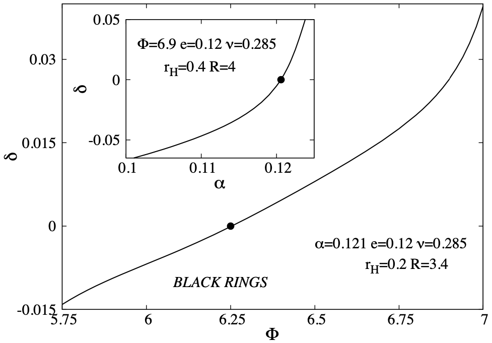
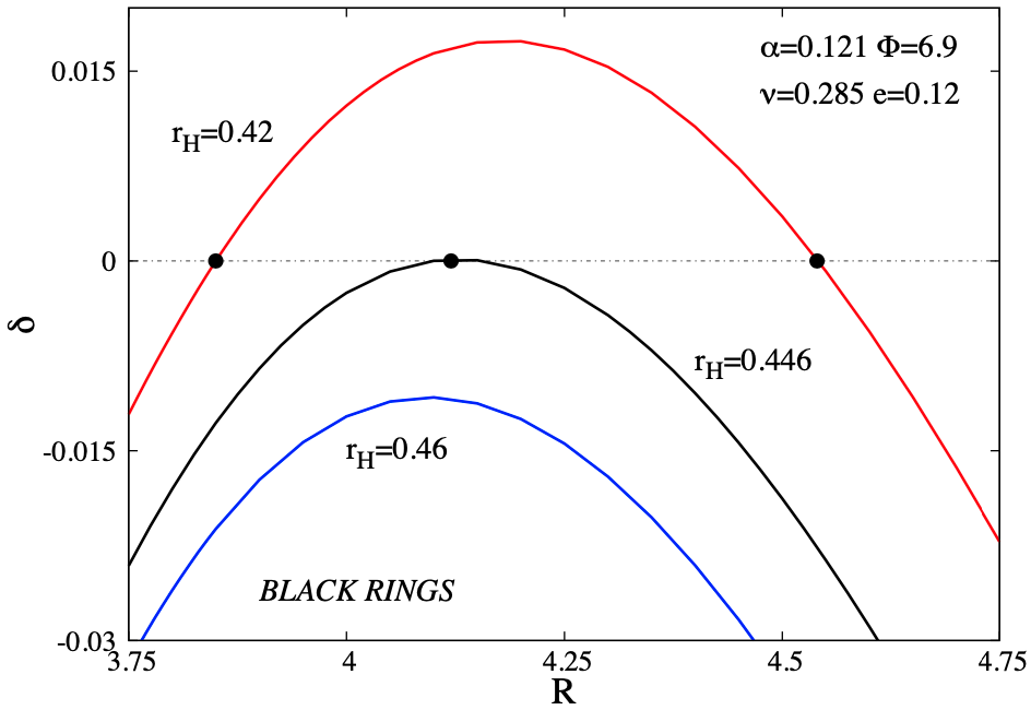
Figure 4: The conical excess/deficit $\delta$ of a static BR in EMgS field theory is shown as a function of the input parameter $\alpha$ which measures the strength of gravity (the inset) and of the electrostatic potential $\Phi$ (left panel), and as function of the ring’s radius $R$ (right panel).

The reported solutions are regular on and outside the horizon and show no sign of a singular behaviour, apart from the generic existence of conical singularities. However, balanced BRs exist as well, requiring a fine-tunning of the input parameters. They are constructed as follows. The starting point are the solutions in the probe limit, $i.e.$ with $\alpha=0$, some values of $(\beta,e;\Phi)$ and a vacuum BR background with parameters $(r_{H},R)$. Then the value of the coupling constant $\alpha$ is increased in small steps. As seen in Figure 4 (inset), the (absolute) value of the conical excess $\delta$ decreases as $\alpha$ is increased. Therefore, for a BR set with fixed horizon and ring radii $(r_{H},R)$, a balanced configuration (marked with a black dot in that figure) is achieved for a critical value of $\alpha$. Further increasing $\alpha$ results in configurations with a conical excess $\delta>0$. Balanced BR exist as well for a critical value of the chemical potential $\Phi$ ($i.e.$ a strong enough electric field) when keeping fixed the other input parameters, see Figure 4 (left panel).

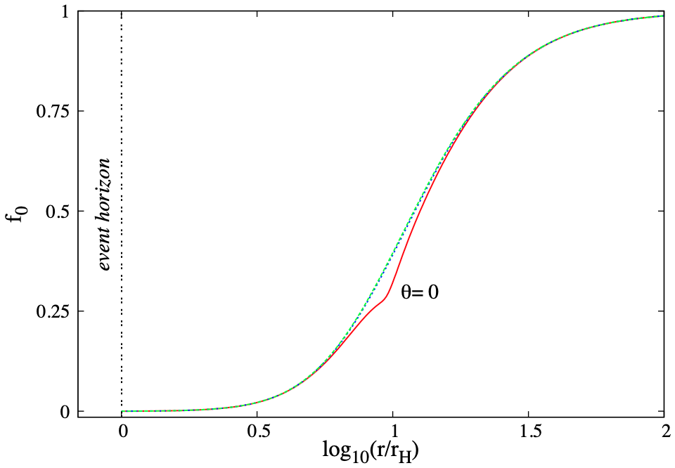
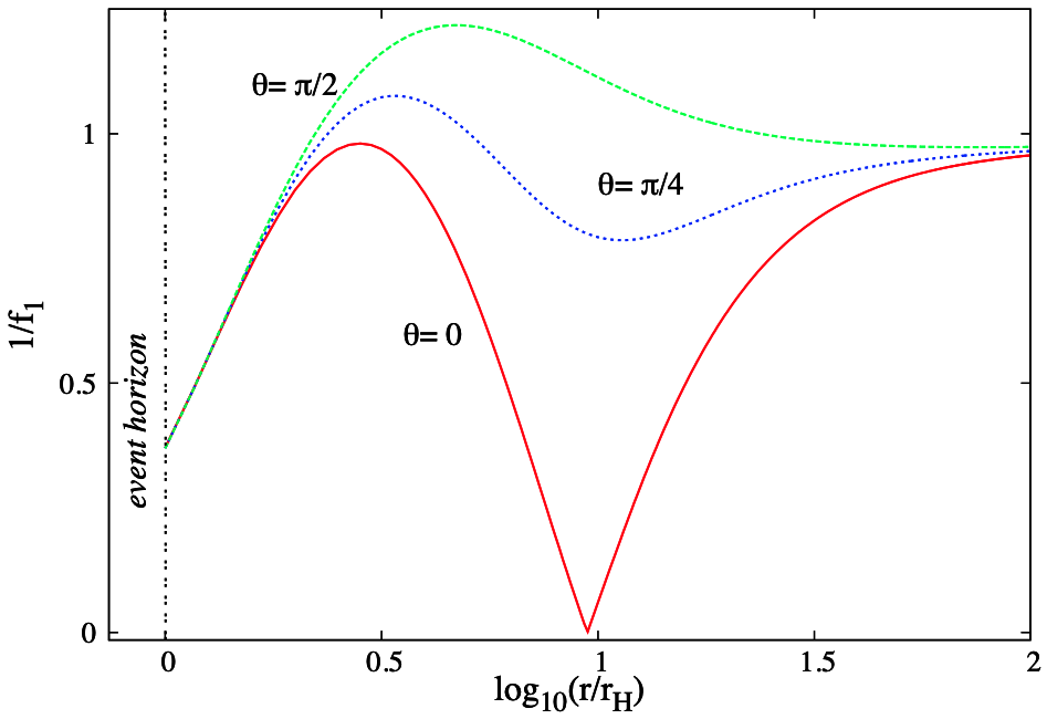
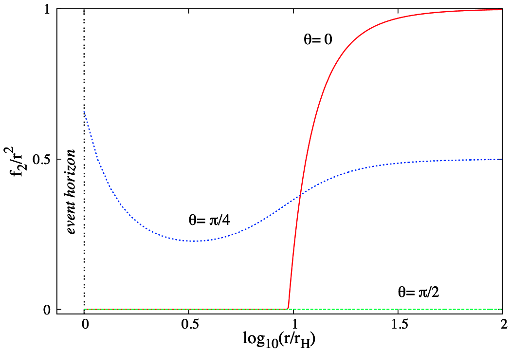
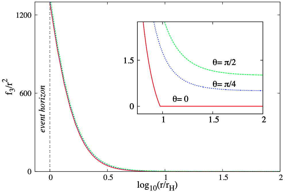
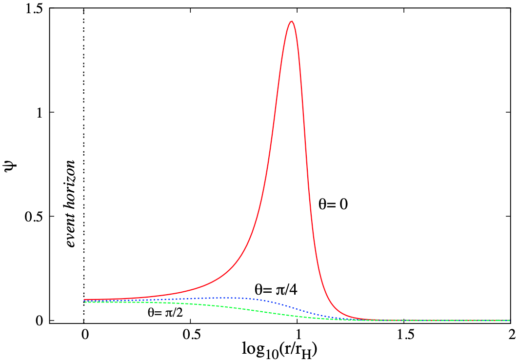
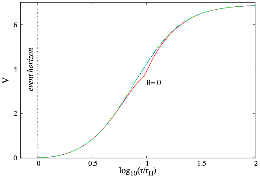
Figure 5: Profile functions of a typical static BR solution with gauged scalar hair are shown for three values of the angular coordinate $\theta$. The input parameters are $r_{H}=0.4$, $R=3.781$ and $\alpha=0.121$, $\nu=0.285$, $\Phi=6.9$, $e=0.12$.

The profile of a typical balanced solution $(\delta=0)$ is shown in Figure 5. As one can see, the functions $f_{i}$ display a complicated behaviour, which, however, is compatible with the imposed boundary conditions, being essentially fixed by the ${f}_{i}^{(0)}$ contribution in (4.14). Also, while the electric potential has a small angular dependence, this is not the case for the scalar field, which possesses a maximum at $r=R$, $\theta=0$. We remark there are no nodes, with $\psi(r,\theta)>0$ not crossing the axis.

In the context of this work, we are interested in solutions with a fixed $\Phi$ and fixed coupling constants $(\alpha>0,\beta,e)$. Then, when varying the size of the ring (via the input parameter $R$) for fixed $r_{H}$, the conical deficit/excess $\delta$ varies as well, which may result in the possible existence of balanced configurations, $\delta=0$. In Figure 4 (right panel) the value of $\delta$ is shown as a function of $R$ for several value of the horizon radius $r_{H}$. One can see that for some range $r_{H}<r_{H}^{(\rm max)}$ the condition $\delta=0$ is satisfied by two different BR solutions (marked with dots in Figure 4). The value of $r_{H}^{(\rm max)}$, however, depends on the choice of other input parameters.

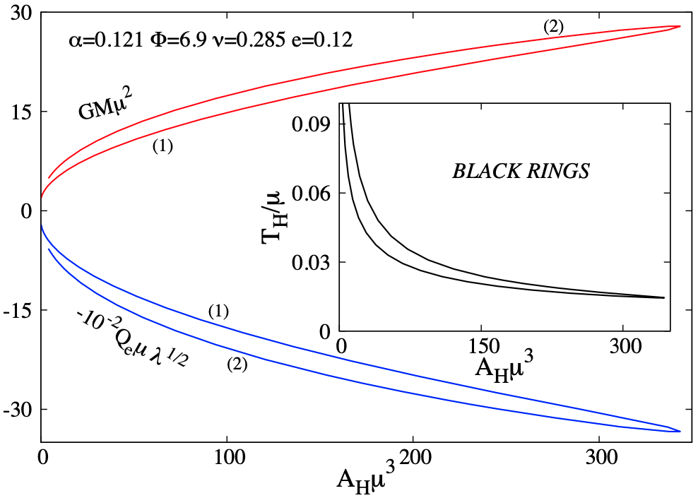
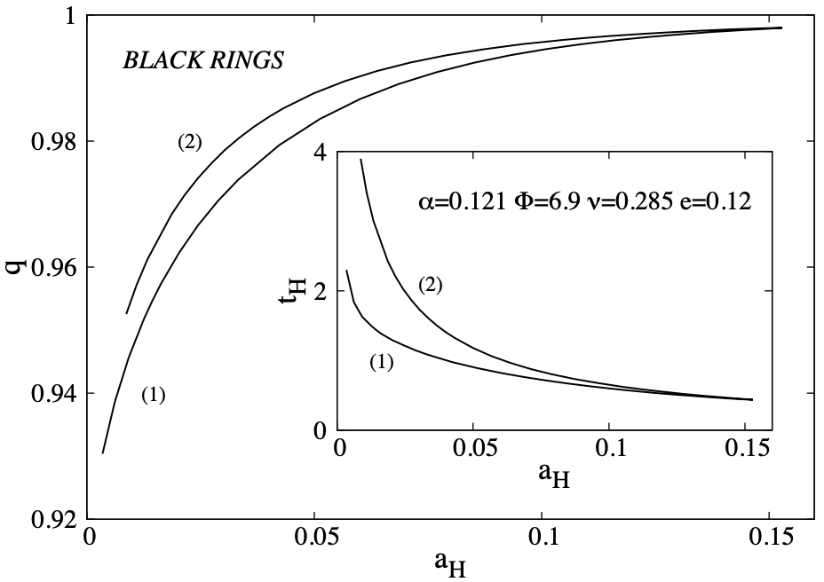
Figure 6: The mass, electric charge and Hawking temperature of solutions are shown as a function of event horizon area for balanced BR solutions.

Some basic features of the solutions with fixed $\Phi$ can already be deduced from Figure 4 (right panel). First, all balanced BRs exist up to a maximal horizon size. That is, no arbitrarily large balanced BRs were found for the cases investigated so far. Second, one notices again the existence of two branches of solutions merging for some maximal horizon size, see Figure 6.

Although further work is necessary, the existing results suggest a strong analogy with the picture found for BHs and BSs. A branch of fundamental solutions (label (1) in Figure 6) emerges from the (spherically symmetric) gravitating gauged $Q$-ball when adding a small horizon with ring topology. As seen in Figure 6, this set stops to exist for a maximal value of the horizon area, with a backbending and the occurrence of a secondary branch. The limiting solution of this branch is unclear, even though the situation appears to be similar to that found in [32] for $D=4$ BHs. That is, the secondary branch stops to exist for a nonzero $A_{H}$, where the numerical results become unreliable, with large violations of the constraint equations.

We expect to find a different picture for other values of the electrostatic potential, with the existence of two branches interpolating between different (spherically symmetric) gauged $Q$-balls. In any case, the presence of scalar hair leads to a very different picture as compared to that found for BRs in electrovacuum, as $e.g.$ seen when comparing Figures 6 (right panel) and 8.

Finally, let us mention that, in the (electro)vacuum case, the spherically symmetric BHs are recovered as the limit $r_{H}\to R$ of the BR solution. However, somehow unexpected, so far we did not find any indication for the existence of such a smooth limit with scalar hair. That is, all EMgS solutions with $r_{H}$ nonzero and close to $R$ possess conical singularities.

5 Summary and overview

In this paper we have reported the first construction of higher dimensional ($D>4$) solutions with charged scalar hair in the literature. Three different types of static solutions have been considered, corresponding to black holes (BHs), black strings (BSs) and black rings (BRs). One of the conclusions of our study is the confirmation that the properties of known $D=4$ BHs [31, 32, 33] are generic, their existence being anchored in the resonance condition (1.1). As a byproduct of our study, we report on the existence of static BRs which are free of singularities, on and outside the event horizon.

As possible avenues for future research, we start with a number of open issues which apply also for the known four dimensional solutions. In our opinion, a main question is to clarify why no hairy solutions could be found in the absence of scalar field self-interaction, $i.e.$ with $\lambda=\nu=0$ in the scalar field potential (2.26). Moreover, it would be interesting to investigate the issue of linear stability of the $D=4,5$ hairy BHs (or for the $D=5$ BSs).

Turning to more general models, we predict the existence of similar solutions for a gauged Proca field. So far only $D=4$ solutions without an event horizon have been discussed in the literature, see $e.g.$ [62].

The status of the EMgS solutions with more general asymptotics is also worth studying. It is interesting to remark that such solutions are known to exist for AdS asymptotics, providing the gravity duals of $s-wave$ superconductors [63]. The main difference $w.r.t.$ the asymptotically flat case is that the AdS solutions emerge as perturbations around a RN-AdS background. Also, the nonlinearities of the scalar field potential play no important role in this context. It would certainly be interesting to look for similar solutions with a positive cosmological constant.

There are also a number of issues specific to higher dimensions. First, it would be interesting to clarify the generality of the resonance mechanism: dos it work for any horizon topology and any dimension $D\geq 4$? Furthermore, for the same matter content and $D=5$, one could consider other type of solutions in Kaluza-Klein theory, such as caged BHs [64, 65] and squashed BHs [66].

Finally, let us mention that the (electro)-vacuum solutions with Kaluza-Klein asymptotics possess the (gravitational) Gregory-Laflamme instability [67], with the additional existence of another set of solutions depending of the compact extra-coordinate, which is $z$ for the background metric (2.20), $i.e.$ nonuniform BSs [69, 68, 70]. On general grounds, we expect the existence of similar solutions in the considered EMgS model.

Acknowlegements

This work is supported by the Center for Research and Development in Mathematics and Applications (CIDMA) through the Portuguese Foundation for Science and Technology (FCT - Fundação para a Ciência e a Tecnologia), references UIDB/04106/2020, UIDP/04106/2020. We acknowledge support from the FCT funded research grants PTDC/FIS-OUT/28407/2017,
CERN/FISPAR/0027/2019, PTDC/FIS-AST/3041/2020 and CERN/FIS-PAR/0024/2021. This work has further been supported by the European Union’s Horizon 2020 research and innovation (RISE) programme H2020-MSCA-RISE-2017 Grant No. FunFiCO-777740.

Appendix A The hairless limit: Black holes, strings and rings in Einstein-Maxwell theory

A.1 The Reissner-Nordström black hole

This is the natural generalizations of the well known four dimensional solution, possessing the same basic properties.

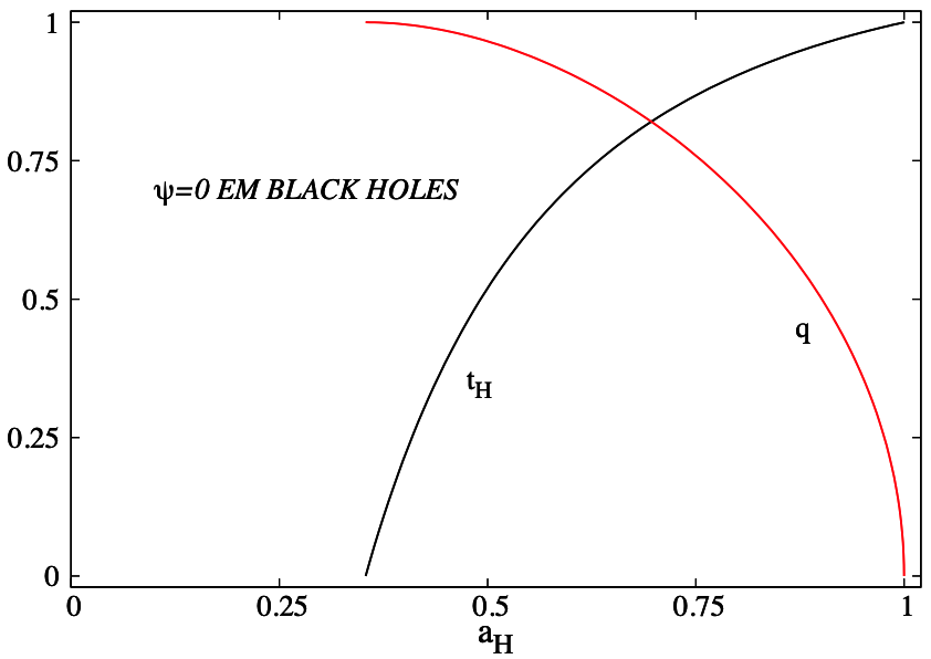
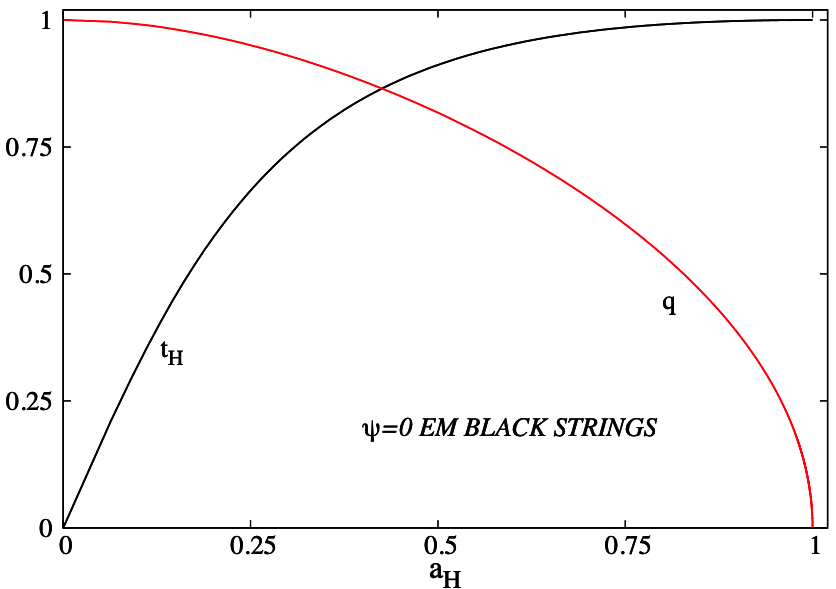
Figure 7: The reduced charge and Hawking temperature are shown as a function of reduced event horizon area for the BH and the BS solutions in Einstein-Maxwell theory.

The line element and the electrostatic potential of the $D=5$ solution reads

$$ds^{2}=-N(r)dt^{2}+\frac{dr^{2}}{N(r)}+r^{2}d\Omega_{3}^{2},\quad N(r)=1-\frac{8G}{3\pi}\frac{M}{r^{2}}+\frac{GQ_{e}^{2}}{3\pi^{3}}\frac{1}{r^{4}},\quad V(r)=\frac{Q_{e}}{4\pi^{2}r_{H}^{2}}-\frac{1}{4\pi^{2}}\frac{Q_{e}}{r^{2}}.~{}~{}{~{}~{}~{}}$$ (A.1)

Instead of $M$, it is convenient to work with $r_{H}$, the event horizon radius (with $N(r_{H})=0$). Then the expressions of various quantities of interest are

$$M=\frac{3\pi r_{H}^{2}}{8G}\bigg{(}1+\frac{GQ_{e}^{2}}{3\pi^{3}r_{H}^{4}}\bigg{)},~{}~{}A_{H}=2\pi^{2}r_{H}^{3},~{}~{}T_{H}=\frac{1}{2\pi r_{H}}\bigg{(}1-\frac{GQ_{e}^{2}}{3\pi^{3}r_{H}^{4}}\bigg{)},~{}~{}\Phi=\frac{Q_{e}}{4\pi^{2}r_{H}^{2}}.$$ (A.2)

The reduced quantities $a_{H}$ and $t_{H}$ as defined by (2.16), can be expressed as a function of the scaled charge $q$, with

$$a_{H}=\frac{1}{2\sqrt{2}}(1+\sqrt{1-q^{2}})^{3/2},\qquad t_{H}=\frac{2\sqrt{2}\sqrt{1-q^{2}}}{(1+\sqrt{1-q^{2}})^{3/2}}.$$ (A.3)

As one can see in Figure 7 (left panel), $a_{H}$ varies between one – the Schwarzschild-Tangherlini limit, with $q=0$, $t_{H}=1$ – , and $1/(2\sqrt{2})$ – the extremal limit, with $q=1$ and $t_{H}=0$.

A.2 The charged black string

The line element and the electrostatic potential of the BS are given by

$$ds^{2}=-\frac{F(r)}{\Omega(r)^{2}}dt^{2}+\Omega(r)\left[\frac{dr^{2}}{F(r)}+r^{2}d\Omega_{2}^{2}+dz^{2}\right],\qquad V(r)=\frac{Q}{2\pi r_{H}}\frac{1}{1+\sqrt{1+\frac{4GQ^{2}}{3\pi r_{H}^{2}}}}\frac{F(r)}{\Omega(r)}\ ,$$ (A.4)

where

$$F(r)=1-\frac{r_{H}}{r},~{}~{}\Omega(r)=1+\frac{r_{H}}{2r}\bigg{(}\sqrt{1+\frac{4GQ^{2}}{3\pi r_{H}^{2}}}-1\bigg{)}~{}.$$ (A.5)

This solution has two input parameters $r_{H}$ and $Q$, with the following expression for various quantities of interest

$$M=\frac{Lr_{H}}{8G}\bigg{(}1+3\sqrt{1+\frac{4GQ^{2}}{3\pi r_{H}^{2}}}\bigg{)},\quad{\cal T}=\frac{r_{H}}{4G},\quad Q_{e}=LQ,\quad T_{H}=\frac{1}{\sqrt{2}\pi r_{H}}\frac{1}{\bigg{(}1+\frac{4GQ^{2}}{3\pi r_{H}^{2}}\bigg{)}^{3/2}},$$

$$A_{H}=\sqrt{2}\pi Lr_{H}^{2}\left(1+\sqrt{1+\frac{4GQ^{2}}{3\pi r_{H}^{2}}}\right)^{3/2},~{}~{}\Phi=\frac{Q}{2\pi r_{H}}\frac{1}{1+\sqrt{1+\frac{4GQ^{2}}{3\pi r_{H}^{2}}}}~{}.$$ (A.6)

From (2.23), we get the following expression of the scaled area, electric charge and temperature:

$$a_{H}=\frac{4\sqrt{2x}(x+\sqrt{1+x^{2}})^{3/2}}{(x+3\sqrt{1+x^{2}})^{2}},\quad q=\frac{1}{\sqrt{1+x^{2}}+\frac{x}{3}},\quad t_{H}=\frac{(x+3\sqrt{1+x^{2}})\sqrt{x}}{\sqrt{2}(x+\sqrt{1+x^{2}})^{3/2}},$$ (A.7)

with $0\leq x<\infty$ an arbitrary parameter. The extremal BS limit is singular in this case, being approached for $x=0$ with $a_{H}=t_{H}=0$ and $q=1$. A $x\to\infty$, the Schwarzschild BS is recovered, with $a_{H}=t_{H}=1$ and $q=0$, see Figure 7 (right panel).

A.3 The static charged black ring

This solution has being reported in [55] in the Einstein-Maxwell-dilaton model and for a ring coordinate system. Here we discuss its basic properties for the coordinate system employed in this work and a vanishing dilaton field.

Its line element and the electic potential reads

$$ds^{2}=-\frac{f_{0}^{(0)}(r,\theta)}{\Omega(r,\theta)^{2}}dt^{2}+\Omega(r,\theta)\left[f_{1}^{(0)}(r,\theta)(dr^{2}+r^{2}d\theta^{2})+f_{2}^{(0)}(r,\theta)d\varphi_{1}^{2}+f_{3}^{(0)}(r,\theta)d\varphi_{2}^{2}\right],$$

$$V(r,\theta)=\sqrt{\frac{3}{16\pi G}}\frac{f_{0}^{(0)}(r,\theta)\tanh\gamma}{\Omega(r,\theta)},~{}~{}~{}{\rm where}~{}~{}\Omega(r,\theta)=\cosh^{2}\gamma-\sinh^{2}\gamma f_{0}^{(0)}(r,\theta),$$ (A.8)

with $\gamma$ an arbitrary real parameter.

The functions $f_{i}^{(0)}(r,\theta)$ $(i=0,\dots,3)$ corresponds to those which enter (static) Emparan-Reall vacuum solution, with the following expression [60]:

$$f_{0}^{(0)}=\frac{\big{(}1-\frac{r_{H}^{2}}{r^{2}}\big{)}^{2}}{\big{(}1+\frac{r_{H}^{2}}{r^{2}}\big{)}^{2}},~{}~{}f_{1}^{(0)}=\frac{\big{(}1+\frac{r_{H}^{2}}{r^{2}}\big{)}^{2}}{\big{(}1+\frac{r_{H}^{2}}{R^{2}}\big{)}^{2}P}\bigg{[}\bigg{(}1+\frac{r_{H}^{4}}{r^{4}}\bigg{)}\bigg{(}1+\frac{r_{H}^{4}}{R^{4}}\bigg{)}-\frac{4r_{H}^{4}}{r^{2}R^{2}}\cos 2\theta+\frac{2r_{H}^{2}}{R^{2}}P\bigg{]},\ \ \ \ \ \ \ \ \ \$$ (A.9)

$$f_{2}^{(0)}=\frac{1}{f_{3}^{(0)}}r^{4}\bigg{(}1+\frac{r_{H}^{2}}{r^{2}}\bigg{)}^{4}\sin^{2}\theta\cos^{2}\theta,~{}~{}f_{3}^{(0)}=\frac{r^{2}}{2}\bigg{[}P+\frac{R^{2}}{r^{2}}\bigg{(}1+\frac{r_{H}^{4}}{R^{4}}-\frac{r_{H}^{2}}{R^{2}}\bigg{(}\frac{r^{2}}{r_{H}^{2}}+\frac{r_{H}^{2}}{r^{2}}\bigg{)}\cos 2\theta\bigg{)}\bigg{]}\ ,$$

where we define

$$P=\frac{r^{2}}{2}\left[\left(1+\left(\frac{R}{r}\right)^{4}-2\cos 2\theta\left(\frac{R}{r}\right)^{2}\right)\left(1+\left(\frac{r_{H}^{2}}{rR}\right)^{4}-2\cos 2\theta\left(\frac{r_{H}^{2}}{rR}\right)^{2}\right)\right]^{1/2}\ ,$$

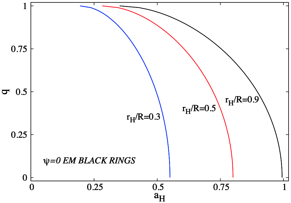
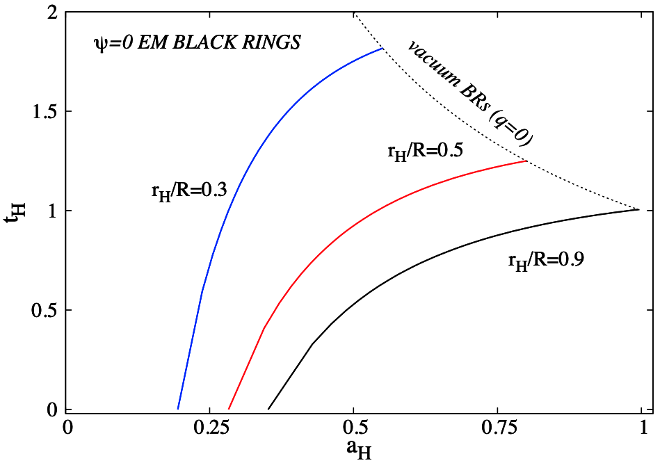
Figure 8: Same as Figure 7 for charged BRs.

with $r_{H}$ the event horizon radius and $R>r_{H}$ the radius of the ring. The vacuum static BR is recovered for $\gamma=0.$ A discussion of the properties this limiting solution for the above parametrization (including the correspondence with the better known Weyl coordinates), can be found in [54, 57]. Here we focused on its charged generalization.

Although the geometry (A.3) is asymptotically flat, it contains a conical singularity for $\theta=0$ and $r_{H}\leq r<R$, with the following expression of $\delta$, as resulting from (4.13):

$$\delta=-\frac{4\pi r_{H}^{2}}{(R^{2}-r_{H}^{2})}<0~{}.$$ (A.10)

Also, the BH limit of the solutions is recovered as $r_{H}\to R$; the BS limit is more subtle, being approached as $R\to\infty$, together with a suitable scaling of $r$, $r_{H}$ and $\gamma$.

The expression of various quantities of interest are

$$M=\frac{3\pi r_{H}^{2}\cosh(2\gamma)}{2G},~{}~{}Q_{e}=\frac{2\sqrt{3}\pi^{3/2}r_{H}^{2}\sinh(2\gamma)}{\sqrt{G}},~{}~{}T_{H}=\frac{1+\frac{R^{2}}{r_{H}^{2}}}{8\pi R}\frac{1}{\cosh^{3}\gamma},$$ (A.11)

$$A_{H}=\frac{32\pi^{2}Rr_{H}^{4}\cosh^{3}\gamma}{R^{2}+r_{H}^{2}},~{}~{}\Phi=\sqrt{\frac{3}{16\pi G}}\tanh\gamma~{}.$$ (A.12)

One can verify that the Smarr relation (2.18) is still satisfied, but not the 1st law (2.17), which requires to introduce an extra term associated with the conical singularity [36, 37].

Concerning the reduced quantities (2.16), both $a_{H}$ and $t_{H}$ can be expressed as a function of the scaled charge $q$, with

$$a_{H}=\frac{x}{\sqrt{2}(1+x^{2})}(1+\sqrt{1-q^{2}})^{3/2},\quad t_{H}=\frac{\sqrt{2}(1+x^{2})}{x}\frac{\sqrt{1-q^{2}}}{(1+\sqrt{1-q^{2}})^{3/2}}\quad~{}{\rm with}~{}\quad x=\frac{r_{H}}{R}.~{}~{}{~{}~{}}~{}~{}$$ (A.13)

In Figure 8 we display the curves $q(a_{H})$, $t_{H}(q)$ for several values of the ratio $r_{H}/R$.

References

- [1] J. D. Bekenstein, [arXiv:gr-qc/9605059 [gr-qc]].
- [2] C. A. R. Herdeiro and E. Radu, Int. J. Mod. Phys. D 24 (2015) no.09, 1542014 [arXiv:1504.08209 [gr-qc]].
- [3] T. P. Sotiriou, Class. Quant. Grav. 32 (2015) no.21, 214002 [arXiv:1505.00248 [gr-qc]].
- [4] J. D. Bekenstein, Phys. Rev. Lett. 28 (1972), 452-455
- [5] A. E. Mayo and J. D. Bekenstein, Phys. Rev. D 54 (1996) 5059 [gr-qc/9602057].
- [6] C. A. R. Herdeiro and E. Radu, Phys. Rev. Lett. 112 (2014), 221101 [arXiv:1403.2757 [gr-qc]].
- [7] C. A. R. Herdeiro and E. Radu, Int. J. Mod. Phys. D 23 (2014) no.12, 1442014 [arXiv:1405.3696 [gr-qc]].
- [8] I. Smolić, Class. Quant. Grav. 32 (2015) no.14, 145010 [arXiv:1501.04967 [gr-qc]].
- [9] O. J. C. Dias, G. T. Horowitz and J. E. Santos, JHEP 07 (2011), 115 [arXiv:1105.4167 [hep-th]].
- [10] Y. Brihaye, C. Herdeiro and E. Radu, Phys. Lett. B 739 (2014), 1-7 [arXiv:1408.5581 [gr-qc]].
- [11] C. Herdeiro, J. Kunz, E. Radu and B. Subagyo, Phys. Lett. B 748 (2015), 30-36 [arXiv:1505.02407 [gr-qc]].
- [12] C. A. R. Herdeiro, E. Radu and H. Rúnarsson, Phys. Rev. D 92 (2015) no.8, 084059 [arXiv:1509.02923 [gr-qc]].
- [13] J. F. M. Delgado, C. A. R. Herdeiro, E. Radu and H. Runarsson, Phys. Lett. B 761 (2016), 234-241 [arXiv:1608.00631 [gr-qc]].
- [14] C. Herdeiro, J. Kunz, E. Radu and B. Subagyo, Phys. Lett. B 779 (2018) 151 [arXiv:1712.04286 [gr-qc]].
- [15] Y. Q. Wang, Y. X. Liu and S. W. Wei, Phys. Rev. D 99 (2019) no.6, 064036 [arXiv:1811.08795 [gr-qc]].
- [16] J. Kunz, I. Perapechka and Y. Shnir, Phys. Rev. D 100 (2019) no.6, 064032 [arXiv:1904.07630 [gr-qc]].
- [17] J. F. M. Delgado, C. A. R. Herdeiro and E. Radu, Phys. Lett. B 792 (2019), 436-444 [arXiv:1903.01488 [gr-qc]].
- [18] C. Herdeiro, E. Radu and H. Rúnarsson, Class. Quant. Grav. 33 (2016) no.15, 154001 [arXiv:1603.02687 [gr-qc]].
- [19] N. M. Santos, C. L. Benone, L. C. B. Crispino, C. A. R. Herdeiro and E. Radu, JHEP 07 (2020), 010 [arXiv:2004.09536 [gr-qc]].
- [20] S. Hod, Phys. Rev. D 86 (2012), 104026 [erratum: Phys. Rev. D 86 (2012), 129902] [arXiv:1211.3202 [gr-qc]].
- [21] S. Hod, Phys. Rev. D 90 (2014) no.2, 024051 [arXiv:1406.1179 [gr-qc]].
- [22] C. L. Benone, L. C. B. Crispino, C. Herdeiro and E. Radu, Phys. Rev. D 90 (2014) no.10, 104024 [arXiv:1409.1593 [gr-qc]].
- [23] S. Hod, JHEP 01 (2017), 030 [arXiv:1612.00014 [hep-th]].
- [24] R. Brito, V. Cardoso and P. Pani, Lect. Notes Phys. 906 (2015), pp.1-237 [arXiv:1501.06570 [gr-qc]].
- [25] W. E. East and F. Pretorius, Phys. Rev. Lett. 119 (2017) no.4, 041101 [arXiv:1704.04791 [gr-qc]].
- [26] C. A. R. Herdeiro and E. Radu, Phys. Rev. Lett. 119 (2017) no.26, 261101 [arXiv:1706.06597 [gr-qc]].
- [27] C. A. R. Herdeiro, [arXiv:2204.05640 [gr-qc]].
- [28] S. Hod, Phys. Lett. B 713 (2012), 505-508 [arXiv:1304.6474 [gr-qc]].
- [29] S. Hod, Phys. Lett. B 718 (2013), 1489-1492
- [30] J. C. Degollado and C. A. R. Herdeiro, Gen. Rel. Grav. 45 (2013), 2483-2492 [arXiv:1303.2392 [gr-qc]].
- [31] J. P. Hong, M. Suzuki and M. Yamada, Phys. Lett. B 803 (2020), 135324 [arXiv:1907.04982 [gr-qc]].
- [32] C. A. R. Herdeiro and E. Radu, Eur. Phys. J. C 80 (2020) no.5, 390 [arXiv:2004.00336 [gr-qc]].
- [33] J. P. Hong, M. Suzuki and M. Yamada, Phys. Rev. Lett. 125 (2020) no.11, 111104 [arXiv:2004.03148 [gr-qc]].
- [34] C. Herdeiro, E. Radu and H. Runarsson, Phys. Lett. B 739 (2014) 302 [arXiv:1409.2877 [gr-qc]].
-
[35]
R. Emparan and H. S. Reall,
Living Rev. Rel. 11 (2008) 6
[arXiv:0801.3471 [hep-th]];
K. Maeda, T. Shiromizu a and T. Tanaka, eds., Higher dimesional black holes, Progress in Theoretical Physics Supplement, 189, (2011);
G. T. Horowitz, ed., Black Holes in Higher Dimensions, (Cambridge University Press, Cambridge, 2012);
H. S. Reall, Int. J. Mod. Phys. D 21 (2012) 1230001 [arXiv:1210.1402 [gr-qc]]. - [36] C. Herdeiro, B. Kleihaus, J. Kunz and E. Radu, Phys. Rev. D 81 (2010) 064013 [arXiv:0912.3386 [gr-qc]];
- [37] C. Herdeiro, E. Radu and C. Rebelo, Phys. Rev. D 81 (2010) 104031 [arXiv:1004.3959 [gr-qc]].
- [38] D. Astefanesei, M. J. Rodriguez and S. Theisen, JHEP 0912 (2009) 040 [arXiv:0909.0008 [hep-th]].
-
[39]
J. H. Traschen and D. Fox,
Class. Quant. Grav. 21 (2004), 289-306
[arXiv:gr-qc/0103106 [gr-qc]];
J. H. Traschen, Class. Quant. Grav. 21 (2004), 1343-1350 [arXiv:hep-th/0308173 [hep-th]]. -
[40]
T. Harmark and N. A. Obers,
Class. Quant. Grav. 21 (2004), 1709
[arXiv:hep-th/0309116 [hep-th]];
B. Kol, E. Sorkin and T. Piran, Phys. Rev. D 69 (2004), 064031 [arXiv:hep-th/0309190 [hep-th]]. -
[41]
U. Asher, J. Christiansen and R. D. Russel,
Math. Comput. 33 (1979) 659;
U. Asher, J. Christiansen and R. D. Russel, ACM Trans. Math. Softw. 7 (1981) 209. - [42] Y. Brihaye and B. Hartmann, Class. Quant. Grav. 39 (2022) no.1, 015010 [arXiv:2108.02248 [gr-qc]].
- [43] Y. Brihaye and B. Hartmann, Phys. Rev. D 105 (2022) no.10, 104063 [arXiv:2112.12830 [gr-qc]].
- [44] P. Jetzer and J. J. van der Bij, Phys. Lett. B 227 (1989) 341.
- [45] P. Jetzer, P. Liljenberg and B.-S. Skagerstam, Astropart. Phys. 1 (1993) 429 [astro-ph/9305014].
- [46] D. Pugliese, H. Quevedo, J. A. Rueda H. and R. Ruffini, Phys. Rev. D 88 (2013) 024053 [arXiv:1305.4241 [astro-ph.HE]].
- [47] A. Prikas, Phys. Rev. D 66 (2002) 025023 [hep-th/0205197].
- [48] Y. Brihaye, V. Diemer and B. Hartmann, Phys. Rev. D 89 (2014) no.8, 084048 [arXiv:1402.1055 [gr-qc]].
- [49] F. R. Tangherlini, Nuovo Cim. 27 (1963) 636.
- [50] R. C. Myers and M. J. Perry, Annals Phys. 172 (1986) 304.
- [51] R. Emparan and H. S. Reall, Phys. Rev. Lett. 88 (2002) 101101 [hep-th/0110260].
- [52] R. Emparan and H. S. Reall, Phys. Rev. D 65 (2002) 084025 [hep-th/0110258].
-
[53]
S. S. Yazadjiev,
[arXiv:hep-th/0507097 [hep-th]];
S. S. Yazadjiev, Phys. Rev. D 73 (2006), 064008 [arXiv:gr-qc/0511114 [gr-qc]]. - [54] B. Kleihaus, J. Kunz and E. Radu, JHEP 1002 (2010) 092 [arXiv:0912.1725 [gr-qc]].
- [55] H. K. Kunduri and J. Lucietti, Phys. Lett. B 609 (2005) 143 [hep-th/0412153].
- [56] B. Kleihaus, J. Kunz and E. Radu, Phys. Lett. B 797 (2019), 134892 [arXiv:1906.06372 [gr-qc]].
- [57] B. Kleihaus, J. Kunz, E. Radu and M. J. Rodriguez, JHEP 1102 (2011) 058 [arXiv:1010.2898 [gr-qc]].
- [58] B. Kleihaus, J. Kunz and K. Schnulle, Phys. Lett. B 699 (2011) 192 [arXiv:1012.5044 [hep-th]].
- [59] B. Kleihaus, J. Kunz and E. Radu, Phys. Lett. B 718 (2013) 1073 [arXiv:1205.5437 [hep-th]].
- [60] B. Kleihaus, J. Kunz and E. Radu, JHEP 1501 (2015) 117 [arXiv:1410.0581 [gr-qc]].
-
[61]
W. Schönauer and R. Weiß,
J. Comput. Appl. Math. 27, 279 (1989) 279;
M. Schauder, R. Weiß and W. Schönauer, The CADSOL Program Package, Universität Karlsruhe, Interner Bericht Nr. 46/92 (1992). - [62] I. Salazar Landea and F. García, Phys. Rev. D 94 (2016) no.10, 104006 [arXiv:1608.00011 [hep-th]].
- [63] S. S. Gubser, Phys. Rev. D 78 (2008) 065034 [arXiv:0801.2977 [hep-th]].
- [64] H. Kudoh and T. Wiseman, Phys. Rev. Lett. 94 (2005), 161102 [arXiv:hep-th/0409111 [hep-th]].
- [65] M. Kalisch, [arXiv:1802.06596 [gr-qc]].
- [66] H. Ishihara and K. Matsuno, Prog. Theor. Phys. 116 (2006), 417-422 [arXiv:hep-th/0510094 [hep-th]].
- [67] R. Gregory and R. Laflamme, Phys. Rev. Lett. 70 (1993), 2837-2840 [arXiv:hep-th/9301052 [hep-th]].
- [68] T. Wiseman, Class. Quant. Grav. 20 (2003) 1137 [arXiv:hep-th/0209051].
- [69] S. S. Gubser, Class. Quant. Grav. 19 (2002), 4825-4844 [arXiv:hep-th/0110193 [hep-th]].
- [70] B. Kleihaus, J. Kunz and E. Radu, JHEP 06 (2006), 016 [arXiv:hep-th/0603119 [hep-th]].