Resonant tides in binary neutron star mergers: analytical-numerical relativity study

Abstract

Resonant excitations of $f$-modes in binary neutron star coalescences influence the gravitational waves (GWs) emission in both quasicircular and highly eccentric mergers and can deliver information on the star interior. Most models of resonant tides are built using approximate, perturbative approaches and thus require to be carefully validated against numerical relativity (NR) simulations in the high-frequency regime. We perform detailed comparisons between a set of high-resolution NR simulations and the state of the art effective one body (EOB) model TEOBResumS with various tidal potentials and including a model for resonant tides. For circular mergers, we find that $f$-mode resonances can improve the agreement between EOB and NR, but there is no clear evidence that the tidal enhancement after contact is due to a resonant mechanism. Tidal models with $f$-mode resonances do not consistently reproduce, at the same time, the NR waveforms and the energetics within the errors, and their performances is comparable to resummed tidal models without resonances. For highly eccentric mergers, we show for the first time that our EOB model reproduces the bursty NR waveform to a high degree of accuracy. However, the considered resonant model does not capture the $f$-mode oscillations excited during the encounters and present in the NR waveform. Finally, we analyze GW170817 with both adiabatic and dynamical tides models and find that the data shows no evidence in favor of models including dynamical tides. This is in agreement with the fact that resonant tides are measured at very high frequencies, which are not available for GW170817 but might be tested with next generation detectors.

I Introduction

Tidal resonances in coalescing compact binaries have been studied for a long time in connection to gravitational-wave (GW) observations Lai (1994); Reisenegger and Goldreich (1994); Kokkotas and Schäfer (1995); Ho and Lai (1999) (See also Mashhoon (1973, 1975, 1977); Turner (1977) for earlier work on tidally generated radiation.) During the coalescence process, the proper oscillation modes of a neutron star (NS) can be resonantly excited by the orbital frequency. For a quasicircular orbit, the energy transfer between the orbit and the mode can change the rate of inspiral and alter the phase of the chirping GWs Ho and Lai (1999). In general, the impact of the tidal resonance on the GWs depends on the duration of the resonance, and it is stronger the slower the orbital decay is. Initial studies focused on the excitation $g$-modes at frequencies ${\lesssim}100\,$Hz, although the effect was found negligible due to the weak coupling between the mode and the tidal potential Lai (1994). In contrast, $f$-modes have stronger tidal coupling but also higher frequencies of order ${\sim}(GM_{A}/R_{A}^{3})^{1/2}$ ($M_{A}$ and $R_{A}$ are the mass and radius of star $A$, respectively), that correspond to a few kilo-Hertz for typical NS masses and radii. These frequencies are too large for the resonance to occur during the inspiral Ho and Lai (1999); their value actually approaching (or being larger than) the merger frequency Bernuzzi et al. (2014a).

Numerical-relativity (NR) simulations of quasicircular neutron star mergers conducted so far do not show decisive evidence for the presence of $f$-mode resonances. One the one hand, some GW models including $f$-mode resonances have been shown to reproduce the NR waveform phasing near merger Hinderer et al. (2016); Dietrich and Hinderer (2017); Steinhoff et al. (2021). On the other hand, the same data can be reproduced at the same accuracy without assuming the presence of a $f$-mode resonance nor additional parameters Bernuzzi et al. (2015a); Dietrich and Hinderer (2017); Nagar et al. (2018); Akcay et al. (2019). Moreover, it is well known that the two NSs come in contact well before the resonance condition is met Thierfelder et al. (2011); Bernuzzi et al. (2012a) (see also discussion below in Sec. II). Interestingly, $f$-mode excitation is instead observed in NR simulations of highly eccentric compact binaries composed of black-hole–NS East et al. (2012) and two NSs Gold et al. (2012); Chaurasia et al. (2018). In these mergers, each close passage triggers the NS’s oscillation on proper modes; the GW between two successive bursts (corresponding to the passages) clearly shows $f$-mode oscillations (see Fig. 5 below). Note however that the excitation does not meet the resonant condition Gold et al. (2012): the close periastron passage exerts a tidal perturbation which excites the axisymmetric ($m=0$) $\ell=2$ mode Turner (1977).

Recent studies after GW170817 Abbott et al. (2017, 2019, 2018) re-considered waveform models with $f$-mode resonances and demonstrated the possibility of GW asteroseismology with binary neutron star inspiral signals Pratten et al. (2020); Ma et al. (2020); Pratten et al. (2021). In particular, the prospect study in Ref. Pratten et al. (2021) demonstrates that neglecting dynamical tidal effects associated with the fundamental mode could lead to systematic biases in the inference of the tidal polarazibility parameters and thus the NS equation of state. Since GW analyses are performed with matched filtering, these studies postulate the validity of resonant models to merger or contact and a sufficient accuracy of the GW template. While it is, in principle, possible to observationally verify the necessity of a $f$-mode resonance model in a particular observation (e.g. via hypothesis ranking), the quality of current GW data and templates at high-frequencies is still insufficient Gamba et al. (2021a). The potential relevance of resonant tides for GW astronomy and the above considerations motivates further detailed comparisons between the current analytical results and numerical relativity simulations.

In this work, we consider state-of-art models for the compact binary dynamics with tidal resonances in the effective-one-body (EOB) framework and critically assess their validity against numerical relativity data. In Sec. II we briefly summarize the effective Love number model proposed in Refs. Hinderer et al. (2016); Steinhoff et al. (2016) (see also App. A) that can be efficiently coupled to any EOB implementation to generate precise inspiral-merger waveforms. This model prescribes a dynamical Love number (or tidal coupling constant) as function of the quasi-circular orbital frequency that, while approaching merger, enhances the effect of tidal interaction. Qualitatively, this effect is known also from studies of tidally interacting compact binaries with affine models Carter and Luminet (1985); Luminet and Marck (1985); Wiggins and Lai (2000); Ferrari et al. (2009, 2012). On physical ground, tidal interactions stronger than those expected by adiabatic and post-Newtonian models are expected towards merger Damour et al. (2012a). For example, early EOB/NR comparisons for quasi-circular mergers found that the description of tidal effects after contact and towards merger requires to enhance the attractive character of the EOB tidal potential in post-Newtonian form Bernuzzi et al. (2012a, 2014b, 2015a). In these studies, it was also pointed out that a key diagnostic to robustly assess tidal effects in NR data is the use of gauge-invariant energetics Damour et al. (2012b).

In Sec. III, we compare different EOB tidal models to selected, high-resolution NR simulations considering both energetics and GW phasing. In particular, in Subsec. III.1 we consider quasi-circular mergers and show that the $f$-mode resonance does not give a cosistently accurate description of both energetics and the waveform. Similarly, in Subsec. III.2 we consider a highly eccentric merger and show that a $f$-mode resonance model does not qualitatively capture the “free-oscillation” feature observed in the frequency-evolution of the NR waveform. Notably however – modulo this effect – the EOB waveform and (orbital) frequency closely follow the NR quantities up to $\sim$ one orbit before merger, attesting to the goodness of the dynamics description provided by the model even for these extreme systems.

In Sec. IV we perform Bayesian analyses and model selection on GW170817 data using the various EOB models introduced in Sec. II. We find that $f$-mode augmented models are not favored with respect to models which only implement adiabatic tidal effects. The $f$-mode resonant frequencis cannot be measured in GW170817, as also observed in Pratten et al. (2020). This is expected, since $f$-mode inference is mostly informative at frequencies larger than ${\sim}1$kHz (for comparable and canonical NS masses), and GW170817 may not contain enough high-frequency information to allow for such a measurement.

Finally, in Sec. V we conclude that, while the $f$-mode model can be effective in improving the agreement between NR and EOB after contact and to merger, it is not clear whether this corresponds to the actual resonant effect or if it is rather an effective description for the hydrodynamics-dominated regime of the merger. Hence, caution should be applied whenever trying to extract actual physical information (i.e., the $f$-mode resonant frequencies) from a matched filtered analysis using templates that include $f$-mode resonances.

Notation.

We use geometrical units, $c=G=1$. We indicate the total binary mass as $M=m_{1}+m_{2}$, the reduced mass as $\mu=m_{1}m_{2}/M$, the mass fraction of star $A$ as $X_{A}=m_{A}/M$, the mass ratio is $q=m_{1}/m_{2}=X_{1}/X_{2}\geq 1$ and the symmetric mass ratio as $\nu=\mu/M$. The EOB variables are mass rescaled,

$$r=R/(GM)\ ,\ \ t=T/(GM)\ ,\ \ \hat{\Omega}=\frac{d\varphi}{dt}\ .$$ (1)

In these variables Kepler’s law is $\hat{\Omega}^{2}=u^{3}$ with $u=1/r$.

Given the dimensionless Love number for star $A$, $k^{\rm(A)}_{\ell}$, the tidal polarizability parameters are defined as

$$\Lambda^{\rm(A)}_{\ell}=\frac{2}{(2\ell-1)!!}C^{2\ell+1}_{A}k^{\rm(A)}_{\ell}\ ,$$ (2)

where $C_{A}=GM_{A}/(c^{2}R_{A})$. The tidal coupling constants of star $A=1$ are given by

$$\kappa^{\rm(1)}_{\ell}=(2\ell-1)!!\,\Lambda^{\rm(1)}_{\ell}\frac{X_{1}^{2\ell}}{X_{2}}\,,$$ (3)

and $\kappa_{2}^{\rm T}=\kappa_{2}^{(1)}+\kappa_{2}^{(2)}$. The $f$-mode frequency with index $\ell$ of star $A$ is indicated as $\omega^{\rm(\ell)\,A}_{f}$, and we use $\bar{\omega}^{\rm(\ell)}_{f\,{\rm A}}=Gm_{\rm A}\omega^{\rm(\ell)}_{f\,{\rm A}}$ (the labels $A$ and $(\ell)$ are sometimes dropped).

II Effective Love number model

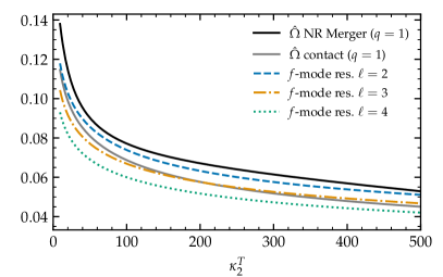
Figure 1: Mass-rescaled orbital merger frequency, contact frequency and resonant conditions for $\ell=2,3,4$ modes for equal-mass binaries with different tidal coupling constant $\kappa_{2}^{\rm T}$. The merger frequency is computed from the NR quasiuniversal fits of Ref. Bernuzzi et al. (2014a). The contact frequency is estimated as in Damour and Nagar (2010) using the quasiuniversal relations $C_{A}(\Lambda_{2}^{\rm(A)})$ of Godzieba et al. (2021).

The model of Refs. Hinderer et al. (2016); Steinhoff et al. (2016) describes the resonant excitation of the NS $f$-mode by a circular orbit based on an effective quadrupolar Love number. The latter is defined by an approximate, Newtonian solution of

$$k^{\rm eff}_{2}=\frac{E_{ij}Q^{ij}}{E^{2}}\,,$$ (4)

where $E_{ij}=\partial_{i}\partial_{j}\phi$ is the external quadrupolar field derived from the Newtonian potential $\phi$ and $Q_{ij}$ is the NS’s quadrupole. The resonance of a NS’s modes is triggered by the condition

$$m\hat{\Omega}\,X_{\rm A}=\bar{\omega}^{\rm(\ell)}_{f\,{\rm A}}\,,$$ (5)

and its net effect is an enhancement of the Love number $k^{\rm(A)}_{\ell}$. This results in a simple prescription to obtain “dynamical tides” based on the formal subsitution of the Love numbers (or equivalently the tidal coupling constants) with their effective values:

$$k^{\rm(A)}_{\ell}\mapsto k_{\ell}^{\rm eff\,(A)}:=\alpha_{\ell m}(\nu,\hat{\Omega},\bar{\omega}_{f\,{\rm A}}^{(\ell)},X_{\rm A})k_{\ell}^{\rm(A)}\,$$ (6)

where the dressing factor $\alpha_{\ell m}$ in Eq. (9) is a multipolar correction valid for $\ell=m$. All the expressions are given in Appendix A.

In this work, the model with $\ell=2,3,4$ resonances is incorporated in TEOBResumS (v3 “GIOTTO”) Damour and Nagar (2014); Nagar et al. (2016, 2018, 2019); Akcay et al. (2021); Nagar et al. (2020); Gamba et al. (2021b); Riemenschneider et al. (2021). Tidal interactions are described by additive contribution $A_{\rm T}$ to the EOB metric potential Damour and Nagar (2010). Different choices for $A_{\rm T}$ are considered: (i) a post-Newtonian (PN) baseline expression including NNLO gravitoelectric corrections Bernuzzi et al. (2012a) (as also employed in Refs. Hinderer et al. (2016); Steinhoff et al. (2016)) and LO gravitomagnetic terms Akcay et al. (2019), (ii) a resummed expression of high-order gravitoelectric $\ell=2$ PN terms obtained from gravitational self-force computations Bini and Damour (2014); Bernuzzi et al. (2015a), hereafter referred as GSF2⁽⁺⁾PN^(-) (See Tab.I of Akcay et al. (2019)); (iii) a resummed expression of high-order gravitoelectric $\ell=2,3$ PN terms obtained from gravitational self-force computations (GSF23⁽⁺⁾PN^(-)). TEOBResumS’s GIOTTO release also includes the LO gravitoelectric PN terms up to $\ell=8$ Godzieba et al. (2021); Godzieba and Radice (2021). Tidal terms in the other EOB potentials and in the waveform are described in detail in Ref. Akcay et al. (2019).

For typical binaries the resonant condition in Eq. (5) is met before the moment of merger (defined as the peak of the $\ell=m=2$ mode of the strain). This is shown in Fig. 1 for equal-mass mergers, where the merger frequency (solid black line) is computed in terms of the tidal coupling constant $\kappa_{2}^{\rm T}$ using the quasiuniveral relations of Ref. Bernuzzi et al. (2014a). The contact frequency (gray solid line) is estimated as in Eq. (78) of Damour and Nagar (2010); this simple expression is known to overestimate the values extracted from the simulations – e.g. $\hat{\Omega}\sim 0.04$ for equal mass NSs with $\kappa_{2}^{\rm T}\sim 180$, effectively corresponding to the last 2-3 GW cycles to the moment of merger Bernuzzi et al. (2012a) – but provides a sufficient estimate for this work.

Colored (non-solid) lines indicate that the resonant excitation for the $\ell=2,3,4$ $f$-mode happens progressively earlier in the merger process. While the $\ell=2$ $f$-mode is excited shortly before merger (approximately corresponding to the last GW cyles) and after contact, the octupolar and hexapolar $\ell=3,4$ mode resonances are reached before the NSs’ contact. This has two important implications. First, the predicted resonance phenomenon can be directly tested with numerical relativity simulations and should, if significant, be visibile in the gauge-invariant energetics of the dynamics from the simulations. Second, the dominant $\ell=2$ resonance happens in a regime in which the model itself is not valid since the NSs are not anymore isolated nor “orbiting”; the matter dynamics being governed by hydrodynamical processes.

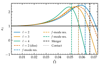
Figure 2: Dressing factors prescribed by the effective Love number model as a function of the orbital frequency and for a fiducial binary. Vertical lines mark the resonances and the merger frequency. The explicit expressions for $\alpha_{\ell m}$ are given in Appendix A. The dashed cyan line is the waveform’s amplitude correction of Eq. (16). The dotted gray line, which happens to be superimposed to the green $\ell=3$ resonance, corresponds to the contact frequency of the stars.

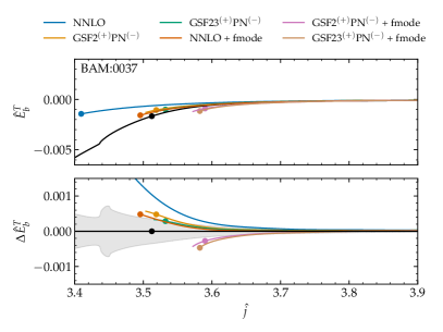
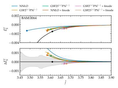
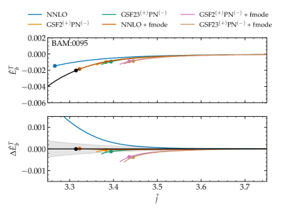
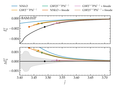
Figure 3: $\hat{E}_{b}^{T}$ and $\Delta\hat{E}^{T}_{b}$ as functions of the angular momentum $\hat{j}$ of the system for the equal mass BAM simulations considered in this paper (black) and the respective TEOBResumS  simulations. The latter are computed using different baseline tidal models (NNLO, GSF2⁽⁺⁾PN^(-), GSF23⁽⁺⁾PN^(-)) and f-mode contributions. The EOB and NR mergers are denoted via dots, while shaded gray bands indicate the NR error.

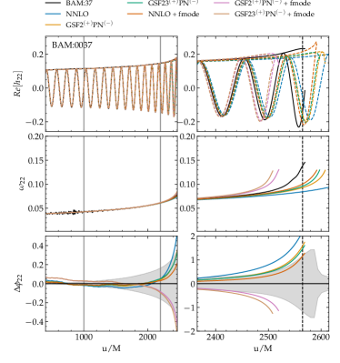
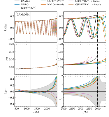
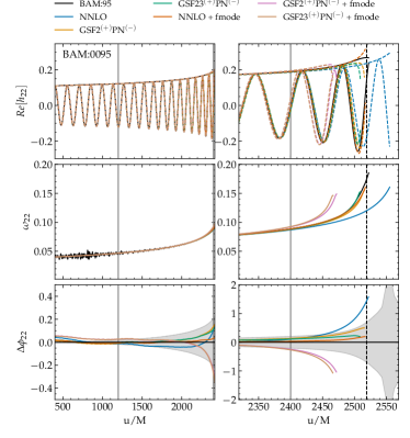
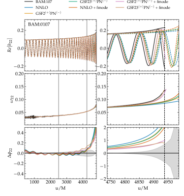
Figure 4: Waveforms (top panels), frequency evolution $\hat{\omega}_{22}$ (middle panels) and EOB/NR phase difference $\Delta\phi^{\rm EOB/NR}$ (bottom panels) for all the non spinning BNS simulations considered in Fig. 3. The GSF+$f$-mode tidal model is the closest to NR for the BAM:0064 and BAM:107 simulations, while for BAM:0037 and BAM:0095 the The NNLO+$f$-mode and the GSF models without dynamical tides deliver the best waveforms.

The typical behaviour of the dressing factors $\alpha_{{\ell m}}$ during the quasi-circular merger process is shown in Fig. 2 for a fiducial binary (that reproduces Fig. 1 of Steinhoff et al. (2016) with our implementation). After the resonance, the dressing factors decrease and become smaller than one or even negative for typical BNS parameters. Since the post-resonance behaviour is not directly modeled in the effective Love number model it is unclear to what extent this effect is physical. However, given that the resonances happen before merger, this trend affects the accuracy of the EOB waveforms that adopt this $f$-mode model.

Indeed, the behaviour of the dressing factors after the resonance can introduce unphysical features in the EOB dynamics by affecting the EOB light ring, $r_{\text{LR}}^{\text{EOB}}$. When using the PN expanded tidal model with dressed tides, the peak of the orbital frequency typically happens after the resonance, i.e. at $\hat{\Omega}_{\rm peak}>\hat{\Omega}_{f}^{(2)}$. Since $\hat{\Omega}_{\rm peak}$ (the EOB light ring) is the natural point to stop the EOB dynamics, the earlier resonance generates an unphysical steep increase of the waveform’s amplitude approaching merger. In order to minimize this behaviour, the EOB model of Hinderer et al. (2016); Steinhoff et al. (2016) terminates the EOB dynamics at the NR merger using the quasiuniversal fits of Bernuzzi et al. (2014a, 2015b) for which $\hat{\Omega}^{\rm NR}_{\rm mrg}<\hat{\Omega}_{\rm peak}$. We follow here the same procedure, but emphasize that this solution is not satisfactory since a well designed EOB model should not break before its light ring (this is true for TEOBResumS even in the binary black hole case). Further, we manually impose that $\alpha_{{\ell m}}\geq 1$ post-resonance.

III Comparison with numerical-relativity data

We contrast different EOB tidal models to selected NR simulations considering both gauge-invariant energy-angular momentum energetics Damour et al. (2012b) and the $\ell=m=2$ waveform mode phasing. We consider the NNLO Bernuzzi et al. (2012a), GSF2⁽⁺⁾PN^(-) Bini and Damour (2014); Bernuzzi et al. (2015a), and GSF23⁽⁺⁾PN^(-) Akcay et al. (2019) prescriptions for the EOB tidal potential with and without the $f$-mode resonance model described above. We consider NR data from quasi-circular and highly eccentric mergers computed respectively in Ref. Dietrich et al. (2017, 2018) and Ref. Chaurasia et al. (2018) using Jena’s BAM code Brügmann et al. (2008); Thierfelder et al. (2011). The binding energy $E_{b}$ and the specific angular momentum $j$ are computed as described in Damour et al. (2012b); Bernuzzi et al. (2012a). The tidal contribution $E_{b}^{\rm T}$ to the energy curves is isolated by subtracting the relative binary-black-hole contribution as described in Bernuzzi et al. (2012a, 2014b, 2015a). For the NR data we use the equal mass, nonspinning binary-black-hole SXS simulation SXS:BBH:0002. For time-domain waveforms comparison, the arbitrary time and phase relative shifts are determined by minimizing the phase difference $\Delta\phi^{\rm EOBNR}$ over a fixed time interval $\Delta t$, e.g. Bernuzzi et al. (2012b); Dietrich et al. (2019).

III.1 Quasi-circular mergers

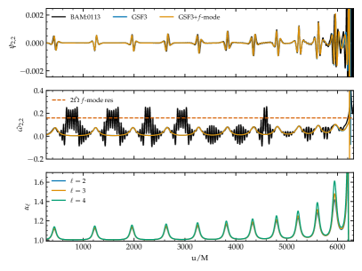
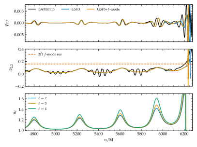
Figure 5: EOB/NR comparison between the multipolar Weyl scalars $\psi_{2,2}$ (top panel) and their respective frequency evolutions $\hat{\omega}_{22}$ (middle panel). The $f$-mode excitations that are typically observed in NR simulations between two close encounters are not captured by the $f$-mode resonance model which prescribes $k_{\ell}\mapsto\alpha_{\ell}k_{\ell}$.

We consider the simulations of the CoRe collaboration named BAM:0037 Dietrich et al. (2017), BAM:0064 Dietrich et al. (2017), BAM:0095 Dietrich et al. (2017) and BAM:0107 Dietrich et al. (2018) corresponding to nonspinning mergers with $\kappa_{2}^{\rm T}=187,287,73,136$ and $q=1,1,1,1.224047$ respectively. These data is computed at multiple resolutions and show convergent properties that allowed a clear assessment of the errobars Akcay et al. (2019). Hence, these are some of the most challenging NR waveforms to reproduce with analytical models.

Figure 3 shows the tidal contribution to the binding energy for the NR data and for all the considered models (top panels) and the differences $\Delta E_{b}^{\rm T}=E_{b}^{\rm T\,EOB}-E_{b}^{\rm T\,NR}$ (bottom panels). The EOB model based on the NNLO PN expansion of the $A_{T}$ potential significantly understimates the actual tidal interaction, as it is well known from previous results Bernuzzi et al. (2012a, 2015a). Augmenting the NNLO model with $f$-mode resonance terms improves the agreement with NR but the energetics are compatible only for BAM:0095 while for the other three binaries the disagreement remains significant. Further, without forcibly stopping the evolution at the NR merger (see Sec. II) the amplitude of the waveform, too, would be largely overestimated near merger. Note the NNLO+$f$-mode is the model employed in SEOBNRv4 Hinderer et al. (2016); Steinhoff et al. (2016, 2021). The GSF2⁽⁺⁾PN^(-) and GSF23⁽⁺⁾PN^(-) models behave very similarly to the NNLO+$f$-mode model, improving the NNLO behaviour but also departing from the NR data for BAM:0064 and BAM:0107. The GSF23⁽⁺⁾PN^(-) is currently the default choice in TEOBResumS Bernuzzi et al. (2015a); Akcay et al. (2019). If these GSF-model are augmented with the $f$-mode the dynamics becomes too attractive and departs from the NR data in all the considered binaries but BAM:0107 and BAM:0064.

Figure 4 shows the GW phasing analysis for all the simulations considered; the top, middle and bottom panel show the evolution of the waveform’s amplitude, the waveform’s frequency and the phase differences $\Delta\phi=\phi^{\rm EOB}-\phi^{\rm NR}$ respectively. For BAM:0107, the frequency evolution of the NNLO model significantly differs out of the alignement interval and is not sufficiently rapid to follow the NR data. This is in agreement with the relative energetics discussed above. The NNLO+$f$-mode and the GSF (without $f$-mode) models improve over the NNLO phasing but, again, the frequency evolution remains too slow to capture the NR tides. On the contrary, the GSF2+$f$-mode models describe very closely the frequency evolution of the NR data, and give the best approximation of the waveform for this binary. This behaviour is consistent with what observed in the energetics above, although the merger – approximated by the EOB light ring – is reached too early in the coalescence.

The BAM:0037 and BAM:0064 phasing analyses are qualitatively analogous to one another, and no model is able to reproduce the NR frequency evolution, although the phase of the corresponding waveform might fall within the NR error. Tidal effects are too attractive for $f$-mode augmented GSF models, and not attractive enough for the remaining models.

Differently from the others, for the BAM:0095 simulation the NNLO+$f$-mode and the GSF (no $f$-mode) models are the closest to the NR data and within the error bars. In this case, the GW phasing analysis is compatible with the results of the energetics.

The results discussed above highlight that establishing the presence of $f$-mode resonances in quasi-circular merger computed in numerical relativity is not straigthforward. On the one hand, the inclusion of this interaction in EOB models can help obtaining analytical waveforms more faithful to NR, at least for some binaries. This is evident in the analysis of the equal-mass, non-spinning merger BAM:0095, where the inclusion of the $f$-mode resonance in the NNLO EOB model shows an excellent agreement to NR data in both energetics and phasing as opposed to the NNLO EOB baseline. On the other hand, the $f$-mode resonance does not capture well the waveforms of other binaries and the EOB/NR waveform agreement does not always correspond to an improvement of the energetics (i.e. the Hamiltonian). For example, the NNLO+$f$-mode model does not perform uniformly well with the other equal-mass, non-spinning binaries. The GSF+$f$-mode models, instead, give a very attractive interaction close to merger and significantly depart from NR for case studies BAM:0037 and BAM:0095.

III.2 Highly eccentric encounters

We consider the BAM:0113 simulation of Ref. Chaurasia et al. (2018), where constraint satsfying initial data are prepared and evolved for a highly eccentric ($e_{\rm NR}\sim 0.45$) merger. The binary undergoes eleven periastron passages before merging; each passage is characterized by a burst of GW radiation, as shown in Fig. 5. Between each burst, the GW shows oscillations compatible with the axisymmetric $f$-mode of the (nonrotating) NS component. The oscillation frequency can be identified also in the fluid density and it is triggered by the close passage to the companion Gold et al. (2012).

TEOBResumS can model these type of mergers Chiaramello and Nagar (2020); Nagar et al. (2021a, b). Although previous works focused on BBH systems, the extension of TEOBResumS to eccentric and hyperbolic binaries including NSs is straightforward, and we have it implemented in this work. The EOB/NR comparison with these type of NR data requires to fine-tune the EOB initial conditions because no analytical map is known between EOB and the initial data employed in the simulation Tichy (2012). In order to reproduce the NR waveform, we fix the NS masses and quadrupolar tidal parameters to those employed in the NR simulation and vary independently the nominal EOB eccentricity and initial frequency until an acceptable EOB/NR phase agreement is found. This procedure is equivalent to fixing the initial frequency of the waveform and varying independently the mean anomaly and the eccentricity of the system. For this work we do not implement a minimization procedure, we instead find that manually tuning the parameters to $\hat{\omega}_{0}=0.0058$ and $e^{0}_{\rm EOB}=0.58$ is enough to obtain a good visual EOB/NR agreement that is sufficient for our purposes.

The waveform comparison is performed in terms of the multipole $\psi_{22}=\ddot{h}_{22}$ of the Weyl pseudoscalar $\Psi_{4}$ since this quantity best highlights the $f$-mode oscillations between the bursts. As shown in the top and middle panels of Fig. 5, the EOB $\psi_{22}^{{\rm EOB}}$ closely matches the NR data in both amplitude and phase showing an excellent agreement during the ten periastron passages and up to merger. However, the middle panel also shows that the EOB $f$-mode model does not capture the high frequency oscillations in the GW frequency $\hat{\omega}_{22}$. This might not be surprising: as shown in the bottom panel of Fig. 5, the $f$-mode model prescribes significant variations of the dressing factors only around the peaks of the (orbital) frequency while it is close to one in-between the peaks. By contrast, in the NR data the high-frequency oscillations are observed mainly at times between two close passages . Further, by comparing the orbital frequency evolution to the resonant frequency condition, we observe that throughout the inspiral the resonance is never fully crossed. To model this behaviour, it seems necessary to consider more complex models which consider the post-resonance dynamics – not included in our effective model – and for which the tidal response is evolved together with the orbital dynamics of the system Turner (1977); Yang et al. (2018); Parisi and Sturani (2018) and incorporate those models in the EOB.

We complement the GW phasing analysis with a discussion on the energetics. Figure 6 shows the binding energy of the highly eccentric system as a function of the orbital angular momentum. The decrease of $\hat{E}_{b}(\hat{j})$ presents clear oscillations that can be reconducted to the close encounters. During each passage both $\hat{E}_{b}$ and $\hat{j}$ decrease but the times at which the two NSs are apart are characterized by approximate “plateaus” (moments of approximately constant energy and angular momentum, see the inset). From this interpretation, it appears that the EOB and NR curves, although close, are not perfectly compatible: the encounters do not always align in the $\hat{E}_{b}(\hat{j})$ curves. Finally, we stress that, modulo the small $f$-mode feature, our EOB waveforms quantitatively reproduce highly eccentric NR simulations up to few orbits before merger. Ours is the first EOB model capable of describing highly eccentric comparable-mass system including neutron stars, and this is to our knowledge the first EOBNR comparison of this kind. The striking agreement between EOB and NR in Fig. 5 attests to the goodness of the radiation reaction model employed within TEOBResumS.

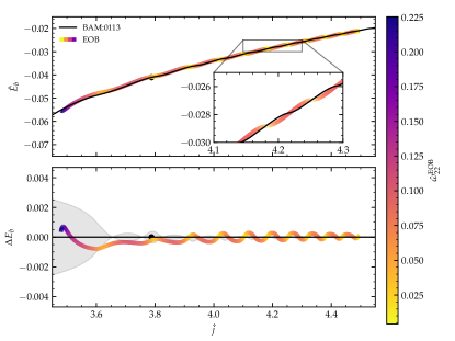
Figure 6: EOB/NR comparison between the evolution of the binding energy $\hat{E}_{b}$ of the system as a function of its orbital angular momentum $\hat{j}$ for the same binary of Fig. 5. The colorbar additionally indicates the EOB frequency evolution along the dynamics. The energy difference that we obtain is $\mathcal{O}(10^{-4})$, compatible with the estimates of the energy carried by $f$-mode oscillations via Eq. 17 of Chaurasia et al. (2018).

IV Model selection on GW170817

We now apply our models to GW170817, using the bajes pipeline Breschi et al. (2021) and the dynesty Speagle (2020) sampler. We consider $128$ seconds of data around GW170817 GPS time, and analyze frequencies between $23$ Hz and $2048$ Hz. The employed prior is uniform in component masses and tidal parameters, isotropic in spin components and volumetric in luminosity distance. It spans the ranges of chirp mass $\mathcal{M}_{c}\in[1.1,1.3]$, mass ratio $q\in[1,3]$, spin magnitudes $\chi_{i}\in[0,0.05]$, tidal parameters $\Lambda_{i}\in[0,5000]$ and distance $D_{L}\in[20,100]$ Mpc. We consider three models for our analysis: the GSF23⁽⁺⁾PN^(-) model, the the GSF23⁽⁺⁾PN^(-) model augmented with dynamical tides and the NNLO model, also augmented with dynamical tides. When using the $f$-mode resonance model, we either fix the values of $\bar{\omega}^{(2)}_{fA}$, $\bar{\omega}^{(2)}_{fB}$ via the quasi-universal relation of Chan et al. (2014) or we infer them independently of $\Lambda$, imposing uniform priors on $\bar{\omega}^{(2)}_{fi}\in[0.04,0.14]$ with $i=A,B$.

Posteriors for the intrinsic parameters can be inspected in App. B. The evidences recovered with the five models are instead reported in Tab. 1. The data mildly favors the GSF tidal model and the GSF model augmented by $f$-mode resonances with respect to the NNLO dynamical tides model. When sampling the resonance frequencies (see Fig 7), we find that it is not possible to precisely determine $\bar{\omega}^{(2)}_{f}$ from GW170817 data. For both tidal baselines, the recovered $\bar{\omega}^{(2)}_{B}$ distribution is consistent with the flat prior imposed. The distribution of $\bar{\omega}^{(2)}_{A}$, instead, allows only to impose an upper or lower bound on the $f$-mode frequency, depending on whether the GSF or NNLO tidal model is employed. This is consistent with what previously observed in Ref. Pratten et al. (2021): it is not possible to accurately determine $\bar{\omega}^{(2)}_{f}$ from GW170817 data.

Table 1: Logarithmic evidences $\log Z$ of the five models employed in our GW170817 reanalysis and their Bayes’ factors computed against the GSF model. The GSF model is slightly favoured over the GSF + $f$-mode model both when we do and do not attempt to infer $\bar{\omega}_{f}^{(2)}$ from the GW data. NNLO + $f$-mode models, instead, appear mildly disfavored with respect to those employing the adiabatic GSF tidal baseline.

Model (X)	$\log{Z}$	$\log{\mathcal{B}^{\rm X}_{\rm GSF}}$
GSF	$480.23\pm 0.18$	$0$
GSF + $f$-mode	$479.61\pm 0.18$	$-0.62$
GSF + $f$-mode + sampling	$479.57\pm 0.18$	$-0.66$
PN + $f$-mode + sampling	$479.22\pm 0.18$	$-1.01$
PN + $f$-mode	$479.15\pm 0.18$	$-1.08$

A simple Fisher Matrix study (Fig. 8) immediately clarifies the reason for the fact illustrated above. Following Ref. Damour et al. (2012a), we compute the diagonal Fisher Matrix (normalized) integrands $\gamma(f)fv^{p}$:

$$\gamma(f)=\frac{f^{-7/3}/S_{n}(f)}{\int_{\rm fmin}^{\rm fmax}f^{-7/3}/S_{n}(f)}\,,$$ (7)

where $v=(M\pi f)^{1/3}$ and $p$ depends on the parameter considered. Employing the PN frequency domain model of Ref. Schmidt and Hinderer (2019) and considering only the leading order for each of the studied parameters, one finds that $p_{\mathcal{M}}=-10$, $p_{\nu}=-6$, $p_{\tilde{\Lambda}}=10$ and $p_{\bar{\omega}_{f}}=22$. This indicates that $f$-mode parameters are determined close to the resonance frequency, where the effect of the model is strongest ($\alpha_{\ell}>1$). For GW170817, such frequencies are dominated by the detectors’ noise.

It is worth noting that in the region where dynamical effects become more prominent (above the frequency of contact between the two stars), the model itself is not physically grounded. PE studies such as the ones presented in Pratten et al. (2020, 2021); Williams et al. (2022) circle this issue by generating waveforms exclusively up to the contact frequency, measuring the secular accumulated phase difference due to the effect of dynamical tides away from the resonance over a very large number of GW cycles. Directly testing the physical validity of this approach is challenging, as it would require extremely long NR simulations which are currently unavailable. Within our EOB model, we find an accumulated phase difference due to dynamical tides of $\sim 0.5-1$ rad at contact for a $1.35+1.35$ reference binary from $20$ Hz (Fig. 9). Most of the phase is accumulated above $300$ Hz. This phase difference might become measurable with third generation detectors Williams et al. (2019), although biases due to an imperfect knowledge of the point mass and (adiabatic) tidal sectors of the models could affect future measurements.

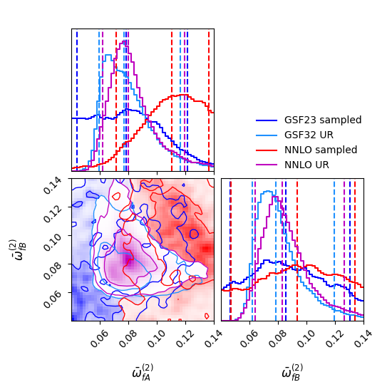
Figure 7: Posterior samples for $\bar{\omega}^{(2)}_{fA}$ and $\bar{\omega}^{(2)}_{fB}$ extracted from GW170817 via direct sampling (blue, red) or by applying quasi-universal relations to the mass and tidal parameters recovered (cyan, magenta). The sampled values span the entire interval investigated, indicating that we are not able to precisely extract the $\ell=2$ resonance frequency from GW170817 data.

V Conclusions

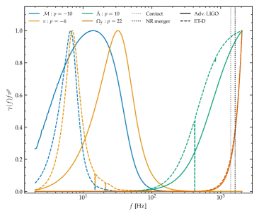
Figure 8: Fisher matrix integrands, computed as in Damour et al. (2012a), evaluated considering the leading order phase contribution for chirp mass, symmetric mass ratio, effective tidal parameter and $f$-mode frequency. Straight curves are computed using advanced LIGO PSD aLI , while dashed lines are estimated with Einstein Telescope PSD Hild et al. (2011). Notably, the $f$-mode resonance frequency is informed mainly by very high frequencies, larger than merger or contact.

In this paper we studied the $f$-mode resonances in three different tidal flavors of the EOB approximant TEOBResumS, namely the NNLO PN, the GSF2 and the GSF23 resummed models. We performed detailed EOB/NR comparisons of both waveforms and gauge-invariant energetics focusing on four selected high-resolution simulations of quasi-circular and one highly eccentric BNS merger.

In the circular merger case, we found that the NNLO+$f$-mode model performs similarly to the GSF-resummed ones without $f$-mode, and that – in all but one case – the model fails to capture either the energetics or the waveform of NR data. Therefore, while the studied model certainly represents a viable alternative to GSF resummation, we suggest caution when trying to extract physical information from it via GW data analysis of real events: no clear signature of the presence of $f$-mode resonances after the NS contact can be assessed from NR simulations.

In the highly eccentric case, we found that the effective $f$-mode model does not capture the oscillations in the NR data (small oscillations in amplitude and frequency of the waveform centered around the proper mode star frequency). This is not unexpected because (i) the $f$-mode model considered here was specifically derived for quasi-circular orbits, (ii) the resonant condition is not met during the close passages. Aside from the small oscillation feature, we demonstrated that our TEOBResumS  for generic orbits quantitatively reproduces the NR waveform and frequency evolution with high-accuracy up to merger. To our knowledge, this is the first EOB/NR comparison of highly eccentric BNS mergers.

Finally, we applied our adiabatic- and dynamic- tidal models to GW170817, and found that models which employ the GSF tides baseline are mildly preferred over models that employ NNLO dynamical tides. Additionally, we were not able to determine $f$-mode resonances from the GW data. The reason for this was immediately understood in terms of a simple Fisher Matrix study, which highlights that dynamical tides are effectively measured at very high frequencies ($\geq 1$ kHz).

Our results should be considered when adopting $f$-mode resonance models in gravitational-wave analyses and parameter estimation. Some of these analyses might be carried with phenomenological models that can reproduce some waveform features but do not allow for a careful check of the underlying dynamics and Hamiltonian Schmidt and Hinderer (2019); Andersson and Pnigouras (2021). A careful validation of these models against more complete EOB models appears necessary in the future.

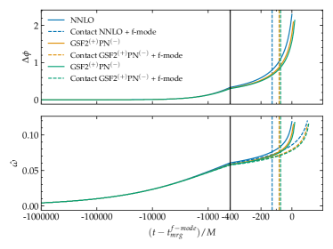
Figure 9: Phase difference $\Delta\phi=\phi^{\rm f-mode}-\phi^{\rm no~{}f-mode}$ due to dynamical tides for a target binary system with $M=2.7M_{\odot}$, $\Lambda_{1}=\Lambda_{2}=978$ and $q=1$ from a starting frequency of $20$ Hz. We employ three different baseline tidal models: NNLO (blue), GSF2⁽⁺⁾PN^(-) (orange) and GSF23⁽⁺⁾PN^(-) (green). Dashed colored lines indicate time of contact between the two stars. Note that the horizontal axis scale changes at $(t-t_{\rm mrg})/M=-400$.

Appendix A Effective Love number model for $f$-mode resonances

This appendix summarizes the effective Love number model introduced in Hinderer et al. (2016); Steinhoff et al. (2016). The model results from an approximate solution of the equation definining the effective quadrupolar Love number

$$k^{\rm eff}_{2}=\frac{E_{ij}Q^{ij}}{E^{2}}\,,$$ (8)

for a Newtonian inspiral. In Eq. (8), $E_{ij}=\partial_{i}\partial_{j}\phi$ is the external quadrupolar field derived from the Newtonian potential $\phi$ and $Q_{ij}$ the NS’s quadrupole. The Love number $k_{\ell}$ of star $A$ (or analogously the tidal polarizability parameter) is substituted with an effective Love number that depends on the orbital frequency and its $f$-mode frequency $\bar{\omega}_{f}^{(\ell)}$,

$$k_{\ell}\mapsto k_{\ell}^{\rm eff}:=\alpha_{\ell m}(\nu,\Omega,\bar{\omega}_{f}^{(\ell)},X_{\rm A})k_{\ell}\,.$$ (9)

The enhancement, or dressing, factor $\alpha_{\ell m}$ in Eq. (9) is a multipolar correction valid for $\ell=m$ and given by

$$\alpha_{\ell m} =a_{\ell}+b_{\ell}\,\left\{\frac{x^{2}}{x^{2}-1}+\frac{5}{6}\frac{x^{2}}{1-x^{5/3}}+\frac{x^{2}}{\sqrt{\epsilon}}\left[\cos\left(\Omega^{\prime}\hat{t}^{2}\right)\int_{-\infty}^{\hat{t}}\sin\left(\Omega^{\prime}s^{2}\right){\rm d}s-\sin\left(\Omega^{\prime}\hat{t}^{2}\right)\int_{-\infty}^{\hat{t}}\cos\left(\Omega^{\prime}s^{2}\right){\rm d}s\right]\right\}\,.$$ (10)

In the above equations, the first multipolar coefficients are $(a_{2},a_{3},a_{4})=(1/4,3/8,29/64)$, $(b_{2},b_{3},b_{4})=(3/4,5/8,35/64)$; the multipolar parameter

$$x:=x_{m}=\frac{\bar{\omega}_{f}^{(\ell)}}{m\hat{\Omega}X_{A}}\,$$ (11)

controls the frequency of the $f$-mode resonance, $\Omega^{\prime}=3/8$ and

$$\epsilon:=\frac{256}{5}\nu\left(\frac{\bar{\omega}_{f}^{(\ell)}}{mX_{A}}\right)^{5/3}\ ,\ \ \ \hat{t}:=\frac{8}{5}\frac{1}{\sqrt{\epsilon}}\left(1-x^{5/3}\right)\,.$$ (12)

The first two terms in Eq. (10) are singular at the resonance ($x=1$). The integrals in the third term reduce to Fresnel integrals

$$F_{S}(z):=\sqrt{\frac{2}{\pi}}\int_{0}^{z}\sin\left(s^{2}\right){\rm d}s\,,\ \ F_{C}(z):=\sqrt{\frac{2}{\pi}}\int_{0}^{z}\cos\left(s^{2}\right){\rm d}s\,,$$ (13)

by writing

$$\int_{-\infty}^{\hat{t}}\cos\left(\Omega^{\prime}s^{2}\right){\rm d}s=\sqrt{\frac{\pi}{2\Omega^{\prime}}}\left[F_{C}\left(\infty\right)+F_{C}\left(\sqrt{\Omega^{\prime}}\hat{t}\right)\right]=\sqrt{\frac{\pi}{2\Omega^{\prime}}}\left[\frac{1}{2}+F_{C}\left(\sqrt{\Omega^{\prime}}\hat{t}\right)\right]$$ (14)

and similarly for the other.

In TEOBResumS, the dressing factors are computed along the dynamics and using the circular frequency $\hat{\Omega}=u^{3/2}$. Following LAL’s SEOBNRv4 implementation of Steinhoff , the singular terms in Eq. (10) are substituted by their expansion near $x=1$ if $x-1<10^{-2}$. The tidal coupling constants are then calculated with the dressing factors and used with any prescription for the EOB tidal potentials. This way, the $f$-mode resonant effect propagates into the EOB dynamics. Spin interactions in TEOBResumS are modeled using the centrifugal radius Damour and Nagar (2014),

$$r_{c}=\left(r^{2}+a_{02}(1+2u)+\Delta_{a2}u+\left(\Delta_{a2}^{\rm NNLO}+\Delta_{a4}^{\rm LO}\right)u\right)^{2}\,,$$ (15)

which include quadrupole $S^{2}$ effects at NNLO and also $S^{4}$ terms. The functions $a_{02}$ and $\Delta$’s contain the quadrupole moments $C_{Q_{A}}$ of the NS; $\Delta_{a4}^{\rm LO}$ also contains the ocutupole and hexapole parameters. The $C_{Q_{A}}$ (and their derivatives) are computed using the fits of Ref. Yagi and Yunes (2013) using the dressed tidal polarizability parameters; no dressing is instead applied to the other parameters for simplicity. Finally, a $\ell=m=2$ waveform’s amplitude correction due to the $f$-mode is applied using the dressing factor

$$\hat{\alpha}_{22}=x^{2}\frac{\alpha_{22}(1+6\frac{X_{B}}{x^{2}})-1}{3(1+2X_{B})}\,.$$ (16)

This result was first reported in Ref. Dietrich and Hinderer (2017) with a different coefficient and without any detail on the calculation. It was later reported with the coefficient used above in Ref. Steinhoff et al. (2021), and it is used in this form also in Steinhoff’s LAL implementation.

Appendix B Posterior plots for GW170817

in this appendix we display the posterior distributions of the intrinsic parameters that we obtained from our GW170817 reanalyses. Figure 10 displays the marginalized two-dimensional posterior samples for the chirp mass $\mathcal{M}$, the mass ratio $q$, the effective spin $\chi_{\rm eff}$ and the tidal parameter $\tilde{\Lambda}$.

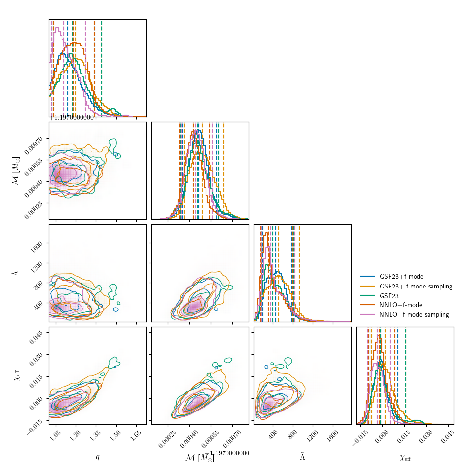
Figure 10: Marginalized, two-dimensional posterior samples for GW170817 obtained with the tidal flavors of TEOBResumS listed in Tab. 1.