Hard X-Ray broadband spectroscopy of Mrk 876: characterizing its spectrum

Abstract

Ever since the launch of the NuSTAR mission, the hard X-ray range is being covered to an unprecedented sensitivity. This range encodes the reflection features arising from active galactic nuclei (AGN). Especially, the reflection of the primary radiation off the accretion disk carries the features of the manifestation of General Relativity described by the Kerr metric due to rotating supermassive black holes (SMBHs). We show the results of the broadband analyses of Mrk 876. The spectra exhibit the signature of a Compton hump at energies above 10 keV and a broadened and skewed excess at energies $\sim$6 keV. We establish this spectral excess to be statistically significant at 99.71% ($\sim$3$\sigma$) that is the post-trail probability through Monte Carlo simulations. Based on the spectral fit results and the significance of spectral features the relativistic reflection model is favored over the distant reflection scenario. The excess at $\sim$6 keV has a complex shape that we try to recover along with the Compton hump through a self-consistent X-ray reflection model. This allows inferring an upper limit to the black hole spin of $a$ $\leq$ 0.85, while the inclination angle of the accretion disk results in $i$=32.84$\degree{}^{+12.22}_{-8.99}$, which is in agreement within the errors with a previous independent measurement ($i$=15.4$\degree{}^{+12.1}_{-6.8}$). While most spin measurements are biased toward high spin values, the black hole mass of Mrk 876 (2.4$\times$10⁸ M_⊙ $\leq$ M_SMBH $\leq$ 1.3$\times$10⁹ M_⊙) lies in a range where moderately spinning SMBHs are expected.
Moreover, the analyses of twelve Chandra observations reveal for the first time X-ray variability of Mrk 876 with an amplitude of 40%.

1 Introduction

Several precise measurements of the cosmic X-ray background (CXB; e.g. Faucher-Giguère, 2020) confirm a common spectral feature: its peak at $\sim$30 keV. Astronomers and astrophysicists agree that most, if not all, of the CXB radiation at its peak is the result of the integrated emission by active galactic nuclei (AGN). Their accretion efficiency, and ultimately their luminosity, strongly depend on the black-hole spin: the more rapidly the black hole spins, the more efficiently it accretes resulting in the spectral Compton hump above 10 keV (George & Fabian, 1991). Its emission peak coincides well with the peak of the CXB. In fact, in a detailed study by Vasudevan et al. (2016) the authors find that 50% of the CXB can be produced by a mere 15% of AGN having a close to maximally spinning supermassive black hole (SMBH). The role of moderately spinning SMBHs remains an open question as half of the spin measurements in AGNs return values close to maximally spinning black holes (spin $a$ $>$ 0.9; Vasudevan et al., 2016). More recent and updated reviews on this subject regarding observational constraints of spin measurements from X-ray data are available in literature (e.g. Reynolds, 2019; Bambi, 2021a; Bambi et al., 2021; Reynolds, 2021). However, this contribution to the CXB might come at the expense of the number of the elusive Compton-thick AGN that have a high column density of the obscuring torus equal or larger to the inverse of the Thomson cross-section (N_H $\geq$ $\sigma$${}_{T}^{-1}$ $\simeq$ 1.5$\times$10²⁴ cm^-2). Such a column density is able to block a large fraction of the radiation from the central region, which in turn hampers the detection of these sources. However, their integrated radiation is predicted to contribute at different percentages in different population synthesis models (e.g. Gilli et al., 2007; Treister et al., 2009; Ananna et al., 2019). Nevertheless, the presence of a large number of Compton-thick AGN could be reconciled with the intensities of both, the CXB and the IR background Comastri et al. (2015). Observational studies with NuSTAR show that the cut-off energy of the continuum characterizes the non-thermal spectrum. Such features are constrained to be well above the Compton hump and even outside the range covered by NuSTAR as shown in individual source studies and for samples of AGN (Fabian et al., 2015, 2017; Tortosa et al., 2018; Middei et al., 2019; Baloković et al., 2020) reinforcing the importance of the Compton hump. Given the reasons above, every case study of broadband measurements to characterize the AGN emission mechanism is of fundamental importance.
Regarding the emission mechanism, the primary radiation is emitted by the hot corona surrounding the SMBH. This is seen as a power-law spectrum by an observer and possibly subject to absorption by the torus depending on the geometric arrangement. This primary radiation also irradiates the accretion disk that reflects it through several reprocessing steps (e.g. Matt et al., 1991) including the fluorescence emission of K$\alpha$ of most abundant elements (George & Fabian, 1991). Most emission lines are unresolved at low X-ray energies resulting in the so-called soft X-ray excess below $\sim$1 keV. Among emission lines from abundant elements in AGN spectra, the most prominent is the Fe–K$\alpha$ line at 6.4 keV. The line can be subject to Doppler shifts, relativistic beaming, and gravitational redshift that can cause distorted line profiles and photon energy shifts (Fabian et al., 2000), which allow for inferring the spin of the SMBH. Additionally, also the electron scattered primary radiation off the inner accretion disk predicted in forma of a broad Compton hump at energies above 10 keV (Ross & Fabian, 1993) can now be measured due to the superb, for this energy band, sensitivity of NuSTAR observations as in Risaliti et al. (2013), whose authors inferred a rapidly rotating black hole. A moderately rotating black hole ($a$ = 0.5) in Swift J2127.4+5654 was discovered by Marinucci et al. (2014) with very deep NuSTAR observations of 340 ksec. Such moderately spinning black holes are important because they represent the missing population in systematic spin measurement studies (Reynolds, 2016). In fact, many sources have lower limits compatible with much higher spin (Vasudevan et al., 2016). Lower spins have not been measured yet, even though low and moderate spins need to be fully accounted for in any population statistics from spin data (Reynolds, 2016) making such spin measurements indispensable pieces in putting the puzzle together. The mass of the SMBH in Mrk 876 has been independently constrained to be between M_SMBH=2.4$\times$10⁸ M_⊙) (Kaspi et al., 2000) and M_SMBH=1.3$\times$10⁹ M_⊙) (Bian & Zhao, 2002). Such a high mass value places Mrk 876 in an interesting parameter space of the mass–spin plane (Vasudevan et al., 2016), where the authors predict intermediate spins can be found.
Mrk 876 is an optically selected Seyfert type-I AGN from the Palomar-Green (PG) Bright Quasar survey (Schmidt & Green, 1983) being often also referred to as PG 1613+658. The source is interacting with another spiral galaxy (Yee & Green, 1987; Hutchings & Neff, 1992). At X-ray energies the source has been detected by Ginga (Lawson & Turner, 1997) and later also at even higher energies in the combined Swift – INTEGRAL X-ray (SIX) survey (Bottacini et al., 2012). Successively also the survey of Swift alone (Baumgartner et al., 2013) has detected the source, while Mrk 876 is not detected in the survey of INTEGRAL. Swift/XRT follow-up observations suggest the source hosts a spinning SMBH measured through a transient gravitationally redshifted Fe line (Bottacini et al., 2015) as measured also in other AGN spectra (e.g. Nardini et al., 2016). The very same analyses of the Swift/XRT observations and analyses of observations by XMM-Newton (Porquet et al., 2004; Piconcelli et al., 2005) reveal the absence of any absorption in excess to the Galactic value.
In this research we present the analyses of the NuSTAR observation on Oct. 22nd, 2020 of Mrk 876 with the aim of characterizing its emission mechanism through its broadband spectrum. The redshift of Mrk 876 $z=0.1385$ (Lavaux & Hudson, 2011) corresponds to 551.4 Mpc for $H_{0}=73$ km s^-1 Mpc^-1 assuming Hubble flow that we do throughout this paper.

2 NuSTAR Observation

2.1 Data Analysis

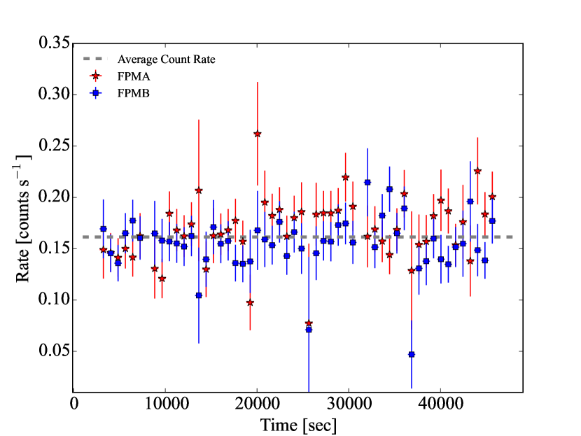
Figure 1: Mrk 876’s light curve binned to 800 seconds for FPMA (red) and FPMB (blue).

The Nuclear Spectroscope Telescope Array (NuSTAR; Harrison et al., 2013) mission has two telescopes that are co-aligned and that have two independent focal plane modules A and B (FPMA and FPMB). The telescopes are able to focus, for the first time, hard X-rays in the energy range 3 – 79 keV allowing for precise imaging and sensitive spectral analyses in this non-thermal energy range.
Since the early days of the mission, Mrk 876 was a target of NuSTAR’s extragalactic survey program EGS, which was later updated with target observations. This observation was performed on 2020-10-22 UT 05:46:09 for $\sim$30 ks with observation id 60160633002. The observation has been analyzed using HEASoft 6.28. Events have been reprocessed with the latest NuSTAR Data Analysis Software (NuSTARDAS v. 1.9.6) using nupipeline and making use of its latest calibration data base (CALDB) files version 20210427. None of the resulting two images are affected by stray-light effect . For the spectral analyses the circular extraction region extends for 60^′′ around the source position, while to maximize the collected background data the area extends for 100^′′ avoiding any overlap with the source.

2.2 Timing Analysis

At hard X-ray energies ($>$ 15 keV) the Swift 105-Month Hard X-ray Survey (Oh et al., 2018) reveals a steady light curve of Mrk 876. By using Swift/XRT and XMM-Newton at lower X-ray energies ($<$ 10 keV) this source has shown some flux variability (factor of $\sim$1.6 at most) on long time scales between 1991 and 2013, while on shorter time scales of weeks, days, and hours the flux is constant (Bottacini et al., 2015). To understand whether the entire integration time of this NuSTAR observation can be used for the spectral analyses, we first explore the variability during the observation. Therefore, the light curve for both detectors is extracted binning the count rate so that every bin lasts for 800 seconds. Such a bin size allows for detecting possible variability trends within the observation frame as in Risaliti et al. (2013). Figure 1 displays the light curve of both modules, FPMA (red stars) and FPMB (blue squares). For comparison, the dashed gray horizontal line is the average count rate. The light curve shows no significant variability in accordance with Oh et al. (2018). Being a Seyfert type-1 AGN, Mrk 876 allows for a rather unobscured view onto the innermost accretion region. In fact, high signal-to-noise XMM-Newton observations ($<$ 10 keV) do not display any absorption in excess to the Galactic value (Porquet et al., 2004; Piconcelli et al., 2005), which excludes also any variability in column density. Furthermore, observations performed by Shull et al. (2011) with the Cosmic Origins Spectrograph aboard the Hubble Space Telescope, confirm a very low column density towards the source. Thus, the spectral analyses capitalize on the entire observation time of NuSTAR.

2.3 Spectral Analysis

To confidently use $\chi$² statistics (Cash, 1979; Gehrels, 1986), NuSTAR data are binned to a minimum of 40 source counts bin^-1. The data are fitted in XSPEC v 12.11.1 (Arnaud, 1996) and errors are properly computed with XSPEC’s error command at 1$\sigma$ level. To all the spectral models used to fit the data, a constant component is added that allows for accounting for the cross-calibration of NuSTAR’s detectors FPMA and FPMB by keeping either fixed to 1, while the other is free to vary. To account for the Galactic absorption towards Mrk 876, assuming solar abundance, the rather precise measurement by Elvis et al. (1989) is used utilizing the NRAO 140 ft telescope of Green Bank finding a value of N${}_{H}^{gal}$ = 2.66 $\times$ 10²⁰ atoms cm^-2 with 5% error, which is in good agreement with the averaged N_H value from the LAB Survey of Galactic H I (Kalberla et al., 2005).

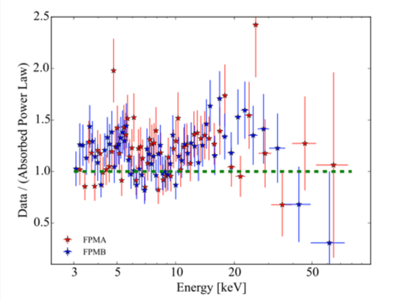
Figure 2: Ratio between data and the folded model, which is an absorbed (fixed to the Galactic value) power-law model (green horizontal line).

Table 1: Spectral parameters of the best fit model for NuSTAR spectrum of Mrk 876. Obs. ID: 60160633002, Obs. Date: 2020-10-22 UT 05:46:09, Obs Exposure: 29969

Model Parameter	Value	Unit
const(wabs(bknpower$+$gauss))
C	1.05${}^{+0.01}_{-0.02}$	…
N${}^{gal}_{H}$	2.6$\times$1020	$atoms~{}cm^{-2}$
$\Gamma_{1}$	1.45${}^{+0.16}_{-0.13}$	…
$\Gamma_{2}$	3.04${}^{+1.76}_{-1.22}$	…
Break Energy	25.95${}^{+5.20}_{-12.82}$	$keV$
Norm (bknpower)	1.50${}^{+1.25}_{-1.15}$	$10^{-4}~{}ph~{}keV^{-1}~{}cm^{-2}~{}s^{-1}$
Line energy	3.72${}^{+1.42}_{-2.03}$	$keV$
Line width	1.42${}^{+0.33}_{-0.31}$	$keV$
Norm (gauss)	8.18${}^{+10.30}_{-6.80}$	$10^{-5}~{}ph~{}s^{-1}~{}cm^{-2}$
Flux${}_{3-79~{}keV}$	1.039${}^{+0.176}_{-0.102}$	$10^{-12}~{}erg~{}cm^{-2}~{}s^{-1}$
$\chi^{2}$	115.54	…
d.o.f.	114	…

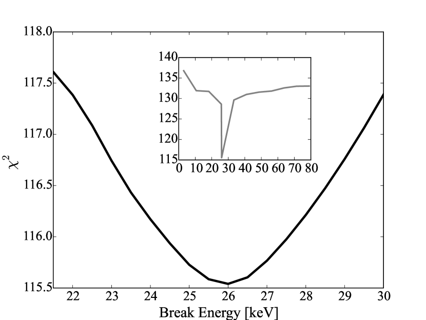
Figure 3: Contour plot of the break energy. The inset shows the minimum to be global.

2.3.1 The Broadband Spectral Analysis

In a first attempt to fit the data, we adopt the simplest spectral shape, which is a power-law model having absorption fixed to the Galactic value (wabs*powerlaw). As a result the fit is unsatisfactory resulting in a reduced chi square of $\chi{{}^{2}}_{red}$=1.15. There is no evidence for further absorption that could improve the fit, which is in agreement with previous studies performed using XMM-Newton and Swift/XRT (Porquet et al., 2004; Piconcelli et al., 2005; Bottacini et al., 2015). The data-to-model ratio of this fit is shown in Figure 2, which displays excesses at energies between $\sim$3.5 – 6.0 keV and between $\sim$10 – 30 keV. To improve the goodness of the fit the broadband is modeled with an absorbed broken power-law model to mimic the excess at high energies. To model the excess between $\sim$3.5 - 6.0 keV an additional broad Gaussian component is added to the model. The complete model is given by an absorbed (fixed to the Galactic value) broken power law plus a Gaussian component (wabs(bknpower+gauss)). Except for the absorption that is fixed to the Galactic value, all parameters are free to vary. As a result this leads to a satisfactory fit being the $\chi^{2}$=115.54 for 114 degrees of freedom. The reduced chi square results in $\chi{{}^{2}}_{red}$=1.01. The complete fit results are reported in Table 1. The break energy of the broken power law is well constrained at E_break=25.95 keV, which is shown in Figure 3 where the break energy on the x-axis constrains the best fit value for the smallest $\chi^{2}$ on the y-axis. The same type of analysis is shown in Figure 4 for the line energy of the Gaussian component, which is also very well constrained. The insets in both, Figure 3 and Figure 4, show that the obtained minimum $\chi^{2}$ is global by scanning the entire parameter space.

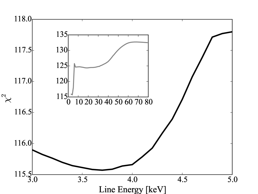
Figure 4: Contour plot of the line energy. The inset shows the minimum to be global.

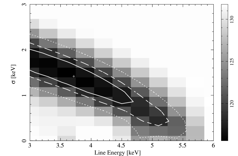
Figure 5: Contours of the line energy (x-axis) and the line width $\sigma$ (y-axis): solid, dashed, and dotted lines delimit the 1$\sigma$, 2$\sigma$, and 3$\sigma$ levels, respectively. The vertical colour bar encodes the values of the $\chi^{2}$ seen as background colour of the figure. The cross (+) at coordinates (3.72, 1.42) represents the best fit value.

For the purpose of visualizing the fit parameters of the Gaussian component, in Figure 5 we show the contour levels of the width of the Gaussian (y-axis) as function of the centroid (x-axis). It is shown that both parameters are independently constrained.
Even though the phenomenological wabs(bknpower+gauss) model precisely fits the data, also the more physically motivated wabs(cutoffpl+gauss) model is being explored. However, such a model worsens the $\chi{{}^{2}}_{red}$ resulting in $\chi{{}^{2}}_{red}$=1.20. By properly computing the fit errors and scanning the parameter spaces the fit improves but the normalization of the Gaussian component remains unconstrained. Very importantly, the cutoff energy at 16.5 keV is found at energies too low for typical values (e.g. Baloković et al., 2020).

2.3.2 Reflection Features off the Accretion Disk and Relativistic Reflection Models

As the Gaussian component might hint at the excess due to the joint effect of Doppler shift, relativistic beaming, and gravitational redshift, its statistical significance needs to be established. There is a general agreement among scientists that line searches driven by observational data must be validated through randomized trials (Protassov et al., 2002). Therefore, we perform Monte Carlo simulations to establish the probability whether the line be a statistical fluke or a real spectral feature. This approach has been extensively used in many researches (e.g. Turner et al., 2010; Tombesi et al., 2010).

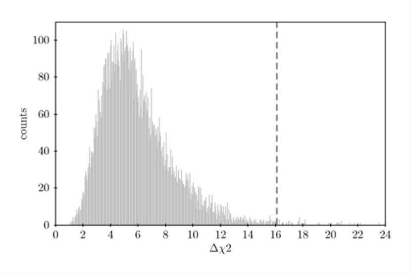
Figure 6: Distribution of $\Delta\chi^{2}$ values obtained with the Monte Carlo simulation. Black dashed vertical line represents the $\Delta\chi^{2}_{thr}$ derived from the actual observation. Three occurrences exceed this value in 10⁴ trials in this simulation thereby rejecting the null-hypothesis at a significance level of $\sim$3$\sigma$ (99.71%), which excludes the broad spectral excess between $\sim$3.5 – 6.0 keV to be a statistical fluke.

Table 2: Spectral fit results of twelve Chandra observations between 2016 and 2017 using the best fit model wabs*bknpower. Fluxes are reported in the range 1-7 keV.

Chandra	Start	Exposure	$\Gamma$1	Ebrk	$\Gamma$2	Norm	$\chi$2	d.o.f.	Flux${}_{~{}1-7~{}keV}$
obs id	[date]	[s]		[keV]		[10-3 ph keV-1 cm-2 s-1]			[10-12 erg cm-2 s-1]
18144	2016-03-18T04:18:40	23920	2.10${}^{2.18}_{2.02}$	4.36${}^{4.86}_{3.99}$	0.20${}^{0.73}_{-0.51}$	1.67${}^{1.77}_{1.56}$	129.73	131	5.26${}^{5.36}_{5.15}$
18145	2016-03-19T22:13:59	23100	2.57${}^{2.87}_{2.35}$	1.60${}^{1.81}_{1.37}$	1.69${}^{1.79}_{1.59}$	1.78${}^{1.91}_{1.59}$	110.17	105	5.18${}^{5.43}_{5.09}$
18146	2016-05-06T06:01:40	22950	2.39${}^{2.59}_{2.21}$	1.75${}^{1.98}_{1.54}$	1.61${}^{1.71}_{1.51}$	1.79${}^{1.90}_{1.68}$	120.38	112	5.58${}^{5.83}_{5.52}$
18147	2016-09-24T16:16:51	11950	2.67${}^{3.04}_{2.33}$	1.65${}^{2.18}_{1.39}$	1.57${}^{1.70}_{1.43}$	1.67${}^{1.43}_{1.70}$	62.94	66	6.35${}^{6.75}_{6.24}$
18148	2017-04-02T03:18:42	17170	2.64${}^{2.90}_{2.35}$	1.59${}^{1.88}_{1.38}$	1.65${}^{1.77}_{1.53}$	1.60${}^{1.73}_{1.46}$	70.93	68	4.63${}^{4.91}_{4.54}$
18799	2016-03-21T00:07:04	24950	2.72${}^{2.95}_{2.48}$	1.54${}^{1.79}_{1.40}$	1.63${}^{1.71}_{1.54}$	1.90${}^{2.01}_{1.79}$	124.61	118	5.58${}^{5.78}_{5.50}$
18814	2016-03-18T23:14:21	23930	2.35${}^{2.66}_{2.24}$	2.63${}^{1.37}_{3.04}$	1.55${}^{1.84}_{1.36}$	2.03${}^{2.15}_{1.91}$	112.94	110	5.44${}^{5.58}_{5.34}$
18844	2016-05-07T09:28:25	22950	2.54${}^{2.78}_{2.35}$	1.76${}^{1.98}_{1.53}$	1.59${}^{1.70}_{1.49}$	1.81${}^{1.93}_{1.70}$	77.48	102	5.30${}^{5.49}_{5.21}$
19885	2016-09-21T01:16:27	25660	2.59${}^{2.86}_{2.38}$	1.62${}^{1.87}_{1.39}$	1.67${}^{1.75}_{1.58}$	2.31${}^{2.43}_{2.18}$	135.84	136	6.68${}^{6.91}_{6.61}$
19889	2016-09-25T20:14:49	12530	2.06${}^{2.15}_{1.97}$	4.44${}^{5.07}_{4.02}$	0.63${}^{1.17}_{-0.19}$	2.13${}^{2.29}_{1.97}$	89.36	96	6.71${}^{6.87}_{6.51}$
20022	2017-03-28T17:08:24	22840	2.73${}^{3.01}_{2.39}$	1.48${}^{1.93}_{1.35}$	1.71${}^{1.81}_{1.60}$	1.74${}^{1.87}_{1.62}$	103.33	94	4.91${}^{5.20}_{4.87}$
20047	2017-03-29T06:15:47	9940	2.98${}^{3.95}_{2.10}$	1.28${}^{2.07}_{1.08}$	1.74${}^{1.86}_{1.56}$	1.63${}^{1.83}_{1.42}$	40.42	41	4.86${}^{5.90}_{4.80}$

To establish the significance of the rather broad excess, Monte Carlo simulations in NuSTAR’s entire energy range between 3 – 79 keV are performed. The null hypothesis for this simulation is: the spectrum measured by NuSTAR is a broken power law with absorption fixed to the Galactic value (null model). This spectrum is simulated with XSPEC using the fakeit command accounting for the instrument’s response files of the actual observation and its exposure. The resulting simulated spectral data are grouped to a minimum of 40 counts bin^-1 as is the measured spectrum of the actual observation. Such a binning allows for an adequate statistics and the confident use of $\chi$² statistics (Cash, 1979). This procedure is iterated 10⁴ times. Each of the spectra are fitted with the null model. The results are used to simulate a further spectrum in the very same way as performed before. This allows for accounting for the uncertainties of the null hypothesis model as described by Markowitz et al. (2006) and by Tombesi et al. (2010). Each obtained simulated spectrum is again fitted with the null model obtaining the $\chi^{2}_{null}$. This will be the reference $\chi^{2}$. The very same simulated spectrum is then fitted with the null model and an additional Gaussian component throughout the range 3 – 79 keV. This energy band is stepped through by energy bins, whose size corresponds to the actual best spectral energy resolution of 0.4 keV of NuSTAR (Harrison et al., 2013). Thus, the simulations will lead to a rather conservative result. During the single fit procedures all parameters are free to float. Especially the normalization value of the Gaussian component varies freely between both, negative and positive values. For each simulated spectrum the best chi square ($\chi^{2}_{best}$) is used to maximize $\Delta\chi^{2}$ (= $\chi^{2}_{best}$ - $\chi^{2}_{null}$). Thus, the distribution of the 10⁴ $\Delta\chi^{2}$ determines the fraction of lines caused by chance fluctuations whenever the value of $\Delta\chi^{2}$ exceeds the threshold value of $\Delta\chi^{2}_{thr}$= 16.09 (131.63 - 115.54) obtained from the actual observation (131.63 and 115.54 being the two $\chi^{2}$ without and with the Gaussian respectively). As a result 29 out of the 10⁴ $\Delta\chi^{2}$ exceed the value of $\Delta\chi^{2}_{thr}$. Therefore, the null hypothesis of the measured spectrum being a broken power-law model with Galactic absorption is rejected with a probability of 99.71%, which corresponds to $\sim$3$\sigma$. This result excludes the broad Gaussian component to be a statistical fluke. The distribution of the 10⁴ $\Delta\chi^{2}$ values is displayed in Figure 6, where the black dashed vertical line represents $\Delta\chi^{2}_{thr}$. Since the modeled excess between $\sim$3.5 – 6.0 keV and the modeled break energy at 25.95 keV improve the fit, we study these rather strong emission features that are typical for relativistic reflection off the accretion disk surrounding the rotating supermassive black hole. These features might be due to the blurring at the accretion disk caused by the strong Doppler and gravitational shifts and by the gravitational redshift. These effects are convolved with the rest-frame X-ray reflection in the widely used self-consistent model RELXILL (version v1.4.3; García et al., 2014; Dauser et al., 2014). This model selfconsiestently accounts for the relativistic reflection physics at work in the vicinity of a black hole. Also it assumes the accretion disk to be irradiated by a power-law coronal emitter. The accretion disk reprocesses the radiation through several steps including the gravitational redshift and the relativistic broadening. By fitting this model to the data, it allows for estimating the accretion disk ionization ($\xi$), the fraction of reflected radiation ($R$), the iron abundance ($A_{Fe}$), the inclination angel of the accretion disk ($\theta$), and the dimensionless spin ($a$), which is allowed to assume values -1 $<$ $a$ $<$ 1 for retrograde and prograde motion. Given the rather short observing time for such an analysis, we approximate RELXILL’s primary radiation to a simple power-law (rather than a broken power law) by equalizing the emissivity index above and below the break making the break itself an unused parameter in this fit. The inferred emissivity index is $q=~{}4.56^{+0.70}_{-0.98}$. The spin results in an upper limit of $a~{}\leq~{}0.85$, while the inclination angle has a rather large error range of $i=32.84$°${}^{+12.22}_{-8.99}$, which however is supported by the inclination angle inferred by Bian & Zhao (2002). For the accretion disk ionization state an upper limit of log($\xi$) $\leq$ 3.17 is inferred, while the iron abundance A_Fe= 1.85${}^{+2.36}_{-1.24}$ is nearly twice the solar value. The reflection fraction has a rather large uncertainty $1.91^{+17.54}_{-1.13}$. The inner radius of the accretion disk in unconstrained, while the outer radius is fixed to 400 gravitational radii.
In the following we also explore the reflection of the primary radiation off material, which is at greater distance from the SMBH. This greater distance from the gravitational potential allows for modeling the spectra without the need of convolving the radiation with relativistic effects. To account for this reflection, we fit the spectra with the xillver reflection model (García & Kallman, 2010; García et al., 2013) in addition to the cutoffpl model to account for the primary radiation. The resulting model is wabs(cutoffpl+xillver). While fitting, the parameters are free to vary and the cut-off energy of the cutoffpl is fixed to the same parameter of the xillver component. The fitted value for this parameter is E_cutoff= 11.59${}^{+12.32}_{-9.06}$, which coincides with the Compton hump. Such cut-off energy is much smaller compared to values routinely found in AGN at energies $\sim$ 200 keV. The inclination angle $i$ and the normalization of the xillver component remain unconstrained.
Additionally we explore the pexmon model (Nandra et al., 2007), which includes also self-consistent lines of Fe K${}_{\alpha},$ Fe K_β and the Compton shoulder (George & Fabian, 1991). A further cutoffpl is added. Also for this reflection fit all the parameters are free to float. The photon index of the pexmon component is tied to the same parameter of the cutoffpl component. Also the two cut-off energies of the two model components are tied. For this model the inclination angle $i$ and the iron abundance A_Fe are unconstrained, while for the cut-off energy a lower limit of E_cutoff>0.01 keV is derived.

2.4 X-ray Observations Below 10 keV

2.4.1 Swift/XRT and XMM-Newton Observations

Observations of Mrk 876 by Swift/XRT and XMM-Newton have been presented in Bottacini et al. (2015). Swift/XRT observations are able to constrain a simple absorbed power-law model only, except for one observation, which displays a transient Fe line at 99% probability. This transient and gravitationally redshifted line originates in a short-lived hotspot on the accretion disk that is due to a magnetic reconnection event in the corona. On the other hand the two XMM-Newton observations are able to constrain a slightly more sophisticated absorbed broken power-law model. The break energy at $\sim$ 1.8 keV and the rise of the spectra toward lower energies might hint at some soft excess, which is in agreement with the two independent analyses by Porquet et al. (2004) and Piconcelli et al. (2005). None of the mentioned analyses including the analysis in Bottacini et al. (2015) detect an Fe line.

2.4.2 Chandra Observations

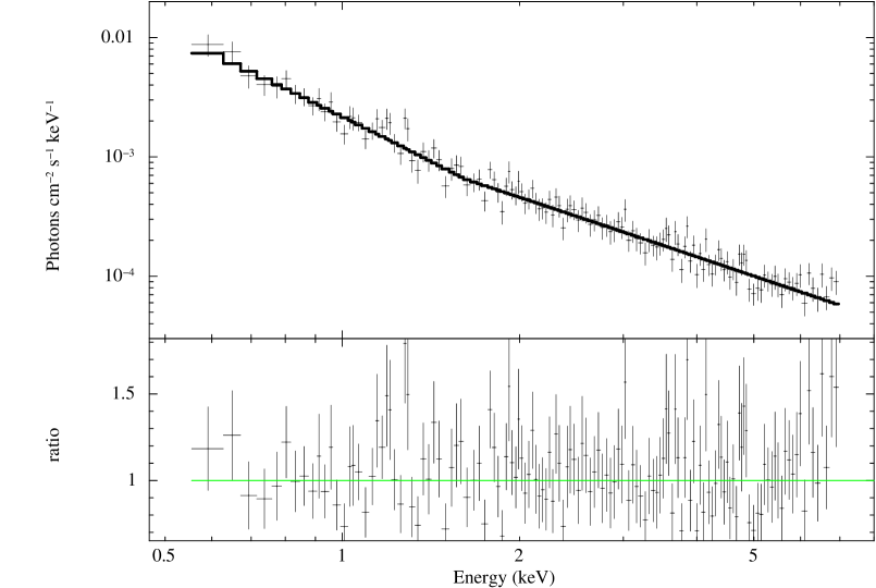
Figure 7: Top panel: Absorbed (fixed to the Galactic value) broken power-law model for Chandra observation 19885. Bottom panel: ratio between data and model.

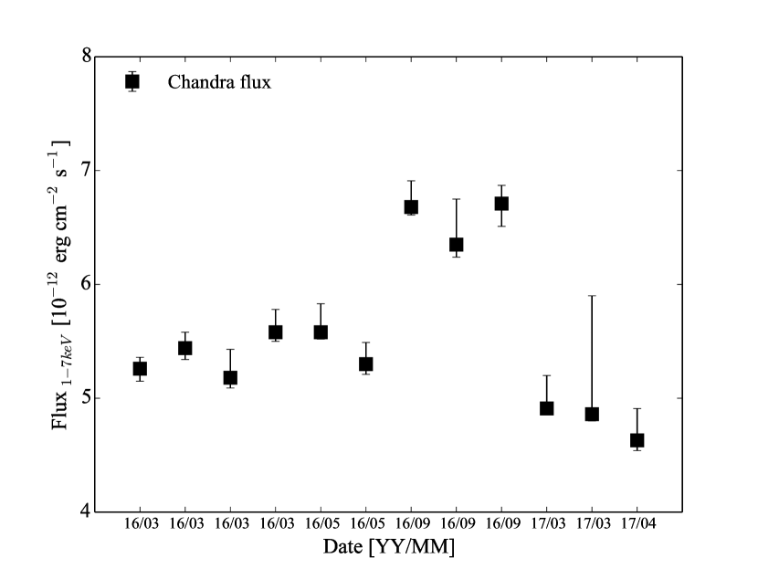
Figure 8: Chandra light curve of Mrk 876 as observed from 2016 to 2017.

The Chandra X-ray Observatory has been monitoring Mrk 876 in the astrophysical context of AGN feedback through outflows with the Advanced CCD Imaging Spectrometer spectroscopic array (ACIS-S) from 2016 to 2017 with 12 observations. These observations have an average exposure time of $\sim$ 20 ksec. Dataset and relevant information can be found in Table 2. These Chandra observations were carried out in FAINT mode. Data have been analyzed using the standard chandra_repro script in CIAO (Fruscione et al., 2006) data analysis system v. 4.13 and Chandra calibration database CALDB v. 4.9.4. Spectra have been extracted with the specextract tool. Additionally they have been binned to contain a minimum of 20 counts bin^-1. Errors are reported at 1$\sigma$ level. All the spectra are best fitted with an absorbed (fixed to the Galactic value) broken power-law model. The break at $\sim$1.6 keV hints at a soft excess, which is consistent with the findings by the observations with XMM-Newton. Figure 7 shows the spectrum of observation id 19885 having a break energy of E_brk=1.6 keV. Observations 18144 and 19889 display a larger break energy of $\sim$4.4 keV. None of the Chandra observations need absorption in excess to the Galactic value, neither at the source nor along the line of sight. This is in agreement with the previous spectral fit results by XMM-Newton and Swift/XRT. Chandra observations detect flux variability that can be pictured in Figure 8. The amplitude of the variability is of 40%. Such variability had not been detected in previous X-ray measurements. While the High-Energy Transmission Grating (HETG) spectrometer with its preferred ACIS-S array (used for these observations) has the ability to spectrally resolve high-velocity outflows and narrow atomic lines, it also is limited to bright sources. Mrk 876 exhibits a moderate flux (average flux in the 1–7 keV band 5.5$\times$10¹² erg cm^-2 s^-1 see Table 2), which might prevent from detecting sharp spectral lines. Neither the very similar observations by XMM-Newton are able to detect sharp spectral features even though its effective area is much larger especially at high energies.

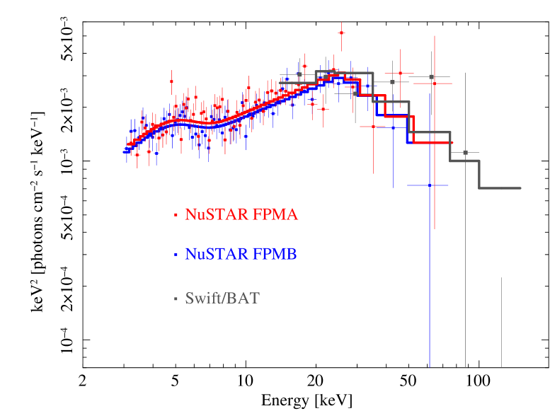
Figure 9: Combined spectra of NuSTAR’s FMPA, FMPB, and Swift/BAT.

2.5 Discussion

As the analyzed data in this research show that Mrk 876 is variable, the combined use of soft X-ray data and NuSTAR data would require simultaneous observations that were actually not performed. However, we compare the flux in the overlapping energy range 3 - 7 keV of the most recent Chandra and NuSTAR observations. The closest observations in time between the two missions (Chandra obs id 18148, which is still $\sim$ 3 years apart) shows the lowest Chandra flux level of 2.4$\times$10^-12 erg cm^-2 s^-1. Yet, this level is more than 20% higher than the flux measured by NuSTAR (1.9$\times$10^-12 erg cm^-2 s^-1), that prevents from fitting the combined datasets.
At the high-end range of the spectrum, the cut-off energy of the continuum emission is routinely found well above 30 keV, at which energy the transfer to the photons is not efficient anymore and the spectrum falls off. This is observationally confirmed by detailed spectroscopic analyses of the Swift/BAT sample that displays a median measured cut-off energy of 76 $\pm$ 6 keV (Ricci et al., 2017). However the same study shows that when accounting also for the lower and upper limits derived from the same sample, the median cut-off energy is even higher at 200 $\pm$ 29 keV. This result has been confirmed very recently with a sample study by Baloković et al. (2020) with the more sensitive NuSTAR measurements. Therefore, it is possible to exclude the spectral turnover at 25.95 keV to be associated to the cut off by the continuum. This becomes apparent from Figure 9 that shows the jointly fitted NuSTAR and Swift/BAT (Oh et al., 2018) spectra with the broken power law plus Gaussian model. BAT data (dark gray markers) extend to somewhat higher energies without detecting the cut-off spectral feature and the break at 25.95 keV represents the data well. Through Monte Carlo simulations, the excess at energies $\sim$3.5 – 6.0 keV has been proven statistically significant to 99.71% (3$\sigma$). This spectral feature and the spectral break at 25.95 keV tie in well with the relativistic disk reflection scenario (Reynolds, 2021, for a very recent review). As an alternative scenario we explore also the warm absorber hypothesis even though Mrk 876’s spectra do not exhibit strong absorption edges. Therefore we fit in addition to the absorbed broken power-law model a warm absorber (zxipcf) (Reeves et al., 2008). Such a model would mimic partially ionized absorbing matter that partially intercepts the primary continuum from the source along the line of sight to the observer. This yields a rather good (although not best) fit result ($\chi{{}^{2}}_{red}$=1.05) even thought the ionization parameter log($\xi$) $=$ 3.0 erg s^-1 and the associated column density N_H $=$ 10²⁴ cm^-2 are physically unsatisfactory values for such intervening matter (Tombesi et al., 2013, and references therein). Both are inconsistent with typical values in the range log($\xi$) $\sim$ 0 – 2 erg s^-1 and N_H $\sim$ 10²⁰ - 10²² atoms cm^-2 (McKernan et al., 2007; Tombesi et al., 2013). Especially this latter value is well established and in good agreement with a recent dynamical modeling of warm absorber motion in AGN (Kallman & Dorodnitsyn, 2019). Such models predict values of N_H to be at most 10²² cm^-2 for small viewing angles as for Mrk 876. Additionally, and very importantly, the warm absorber scenario is unable to account for the spectral break at 25.95 keV. A further issue for the warm absorber scenario comes from the result of the fitted values themselves. In fact, if intervening matter of N_H $\sim$ 10²⁴ cm^-2 would cross the line of sight, then the inevitable efficient absorption would lead to detectable variability on short time scales as warm absorbers are found at velocities $v$ $>$ 100 km s^-1 (Laha et al., 2014) up to mild relativistic velocities (e.g. $\sim$0.3c; Braito et al., 2007). Such variability has never been detected in many observations for Mrk 876 including the present NuSTAR and Chandra observations of this research. Also the neutral Compton reflection off clumpy and optically thick distant clouds would imply absorption variability (Turner et al., 2000; Miller et al., 2008) never observed in Mrk 876.
We also study the distant reflection scenario, whose distinct feature would be a narrow (rather than a large) Gaussian component. To explore the distant reflection scenario the combined use of the cutoffpl and xillver components are unable to constrain the inclination angle $i$. Also the inferred value of the cut-off energy (E_cutoff=11.59 keV) is much lower than the typical values inferred through observations (e.g. Ricci et al., 2017; Baloković et al., 2020). However, this does not come as a surprise. In fact, the cutoffpl in addition to a Gaussian is unable to properly fit the spectra ($\chi_{red}^{2}$=1.20, see section 2.3.1). The same limitations apply to the cutoffpl+pexmon model. Furthermore, also this model does not allow for constraining the inclination angle $i$.
As very recently discussed by the authors of Kamraj et al. (2022), measurements of the cut-off energy should be taken with a skeptical attitude because the values of such measurements are largely affected by the uncertainties in modeling the data and by the quality of the data. Even more so, a such low cut-off energy as inferred in our distant reflection is not measured by current most sensitive observations with NuSTAR (for a sample study see Kang & Wang (2022) and for a case study see Baloković et al. (2021)) nor is it expected theoretically. From a theoretical view, the inverse-Compton scattering of thermal seed photons arising from the accretion disk by the energetic particles of the corona is described by the Kompaneets equation (Kompaneets, 1957). Its solution by Lightman & Zdziarski (1987) and by Zdziarski et al. (1996) predicts a power-law spectrum $N(E)=KE$^-γ, for which the spectral index is given by:

$$\alpha=\sqrt{{9\over 4}+{1\over(kT/m_{e}c^{2})\tau(1+\tau/3)}}-{3\over 2}$$ (1)

where $T$ is the coronal temperature and $\tau$ is the optical depth to the Thomson scattering. This equation holds true for X-ray continua at photon energies much less than the coronal temperature. For higher photon energies the spectrum falls abruptly off, because the electrons of the corona are not energetic enough to up-scatter a large number of photons. Since hard X-ray surveys (e.g. Vasudevan et al., 2013) find temperatures well above 100 keV, much lower cut-off measurements as for our distant reflection model are not justified. To further explore the cut-off energy for the distant reflection, we model this emission scenario by applying a similar value of the reflection fraction as inferred with the RELXILL model ($\Gamma$$\sim$2). This value affects mostly the high-energy component of the spectrum and thereby also the cut-off energy. Indeed, by modeling the distant reflection (cutoff+xillver) with this approach the xillver component dominates over the cutoff component. The normalization of this latter component cannot be constrained by the fit and the value of the cut-off energy shifts to lower values of E_cutoff$\sim$9 keV. Therefore, even by enhancing the contribution of the reflection component, the cut-off energy cannot be found at values that are justified by theory or observations. On the other hand, the relativistic reflection scenario is able to naturally reproduce the broadband spectral features observed with NuSTAR and shown in Figure 10. These spectral features largely depend on the spin of the central supermassive black hole. In Mrk 876 its spin was already put forward (Bottacini et al., 2015) in the context of the transient hotspot scenario (Nayakshin & Kazanas, 2001; Turner et al., 2002) very similar to a precise time-resolved study by Nardini et al. (2016).
Given the above evidences, it is reasonable to fit Mrk 876’s NuSTAR spectra with a more sophisticated model that incorporates the physics of the accretion disk in the vicinity of the black hole, even though the relativistic reflection features are already mimicked and fitted by using the model given by the sum of the broken power law and the large Gaussian component for the low energy part. These features can be reproduced by fitting the RELXILL model that accounts for the entire energy band from 3 – 79 keV. This model constrains the spin to an upper limit of $a~{}\leq~{}0.85$ and the inclination angle of the disk is $i$=32.84°${}^{+12.22}_{-8.99}$. The inclination angle is in agreement with an independent measurements by Bian & Zhao (2002). By using this more sophisticated spectral model we note that some parameters remain unconstrained because of the well known degeneracies among parameters of such models (Reynolds, 2021) and because of the moderate signal-to-noise observation (for such analyses), which however is enough to detect the actual relativistic reflection features. The properly computed uncertainties cannot be significantly reduced by fixing parameters during the fitting process. Therefore, also any discussion to better comprehend the physics at work in the environment of the emission region would lead to speculative conclusions. It is noteworthy that the inferred index of the emissivity profile, which was approximated to a simple power law, is rather steep ($\sim 4$). Such steep values are in agreement with theoretical results related to the effects by gravitational light bending in the vicinity of spinning black holes (Miniutti et al., 2003).

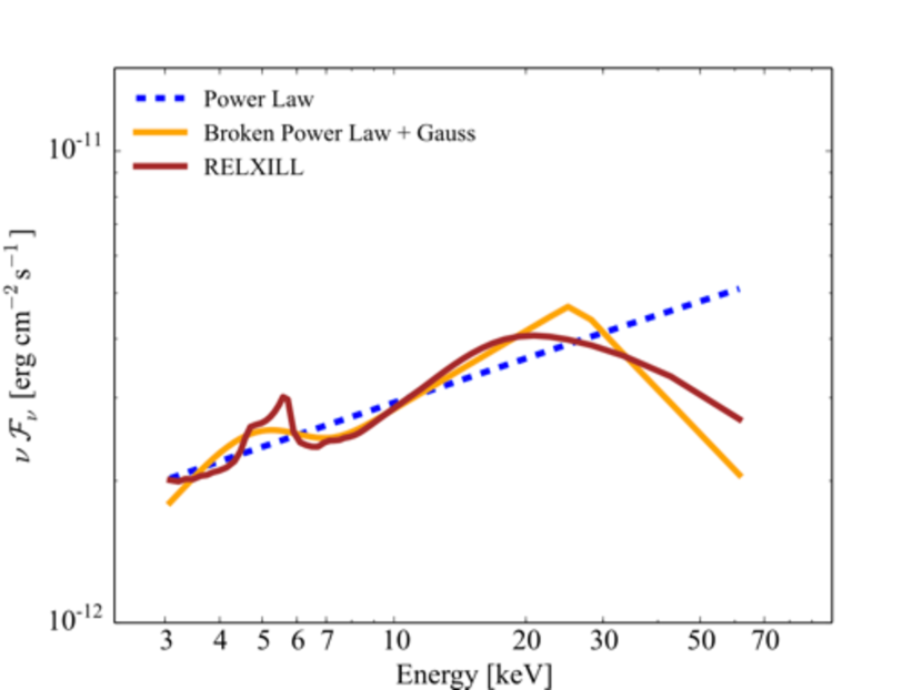
Figure 10: SEDs in form of $E^{2}$$\times$$f(E)$ of the best fit model (broken power law + Gaussian, orange), RELXILL (brown), and simple power law (dashed blue).

Figure 11 shows a comparison of the residuals obtained through the fit results using the previously discussed models. The top panel displays the residuals with respect to the simple power-law fit. The second panel from the top shows that the sum of the broken power law and the Gaussian is able to resemble well the overall broadband spectrum. However, it leaves some excess residuals between 5 – 6 keV behind. In this interval the excess rises towards increasing energies only to fall off abruptly. In the view of the rotating black hole this feature could hint at the red wing of the accretion disk. This feature is largely mitigated in the third panel (RELXILL) from the top. Indeed, Figure 10 displays the two models and also the simple power-law model for comparison. It is apparent that even though the self-consistent reflection model (solid brown) is affected by some statistically unconstrained parameters, it is able to reproduce the best fit model (solid orange). These two models depart from the pure power-law model (dashed blue) to resemble the break at $\sim$26 keV and the excess between $\sim$3.5 – 6.0 keV. This latter feature aligns with the cosmologically redshifted Fe K-shell line system in the rest frame band 6.4 – 6.97 keV. This line system tends to a noticeable red wing, which is the extent of the line to low energies, because the inclination angle of the accretion disk (with respect to the line of sight) is modest ($\sim 30\degree{}$; Fabian et al., 2000; Reynolds, 2021). This can be pictured in the spectral residuals in Figure 11 first two panels from top. The extent to lower energies decays smoothly. To further investigate this spectral feature, a broken power-law model plus a narrow (rather than a broad) Gaussian line to reproduce the excesses of the residuals is being fitted. By properly tuning the initial line energy ($\sim$5.5 keV), the resulting fit leads to a good $\chi_{red}^{2}$=1.12. However, when computing the errors, the fit clearly does not allow for constraining the parameters of the line, which hints at the fact that the line might be broadened and skewed through the joined action of the relativistic Doppler shift and the relativistic beaming. We examine the parameter space of the line width and its energy (i.e. position of the centroid) calculating the corresponding $\chi^{2}$. We show the contours of these two line parameters in Figure 12 where the dark shaded area encodes low $\chi^{2}$ values for larger values of the line width and for smaller values than 5.5 keV of the line energy. Therefore, the line is allowed to shift towards lower energies and the line width can become larger only to obtain equally good fit results. This highlights that the complex Fe-line system decays smoothly towards lower energies hinting at the previously mentioned red wing as manifestation of the joint effects close to the black hole leading to a broadened and skewed shape. We also explore the statistical difference between the narrow and the broad Gaussian used in addition to the broken power-law model. To establish the statistical significance of this narrow component we perform the very same Monte Carlo simulations used for the broad component however keeping the fitted line width fixed to its best value. As a result the difference in $\chi^{2}$ is significant to only $\sim$50%.

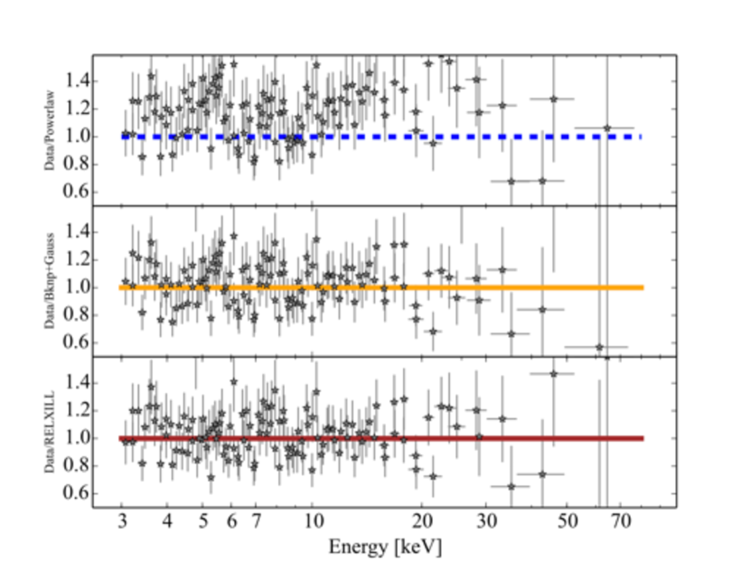
Figure 11: Residuals (data/model) from top to bottom for the following models: powerlaw (dashed blue), bknp+Gauss (orange), RELXILL (brown), where bknp stands for broken power law.

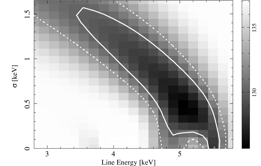
Figure 12: Contours of the line energy (x-axis) and the line width (y-axis): solid and dashed lines delimit the 1$\sigma$ and 2$\sigma$ levels, respectively. The vertical colour bar encodes the values of the $\chi^{2}$. The star at $\sim$ 5.5 keV represents the best fit value.

2.6 Conclusion

This research investigates Mrk 876’s broadband spectrum as observed by NuSTAR. NuSTAR’s spectra have been rebinned so that sharp spectral features are not smoothed out. This is important when exploring the spectral results that show excesses with respect to a simple power-law model, which are characteristic for the reflection of the primary radiation off the accretion disk. A turn over of the broadband continuum at 25.95 keV is interpreted as the Compton hump, while the broad excess at low energies is coincident with the Fe K-shell emission line system. These excesses are less well fitted by distant (from the SMBH) reflection models, which would produce a narrow Fe line feature, rather than a broad feature. In fact, the observed excess around the Fe line energy is best fitted by a broad ($\sigma$=1.4 keV) Gaussian component, which is statistically significant at 99.71% ($\sim$3$\sigma$) being the post-trial probability through Monte Carlo simulations. The fit with a narrow component is significant to only $\sim$50%. This excludes the broad excess at low energies to be a statistical fluke. A further complication for the distant reflection is the low value of the cut-off energy at E=11.59 keV, which is inconsistent with theory and with current most sensitive measurements with NuSTAR. The study of the low-energy excess shows that this system has a complex structure displaying the red wing underpinning the possible combined effect of relativistic Doppler shift, relativistic beaming, and gravitational redshift. The reflection model RELXILL (version v1.4.3; García et al., 2014; Dauser et al., 2014) represents the data rather well even though some parameters remain unconstrained returning an upper limit for the black hole spin of $a$ $\leq$ 0.85, while the inclination angle of the accretion disk results in $i$=32.84°${}^{+12.22}_{-8.99}$, which is in agreement within the errors with a previous independent measurement ($i$=15.4$\degree{}^{+12.1}_{-6.8}$) by Bian & Zhao (2002). To confidently derive the parameters through the sophisticated reflection model, high-quality spectra are needed. Indeed, this NuSTAR observation is of rather low exposure ($\sim$30 kses) for such measurements, which prevents from obtaining well constrained fit parameters, even though this model resembles well the best fit model (see Figure 10). Especially the low-energy excess is well fitted by this model when comparing the residuals (see Figure 11) thereby modeling the data due to the red wing. For the spin measurement, Mrk 876’s SMBH falls in an rather unique mass range (2.4$\times$10⁸ M_⊙ $\leq$ M_SMBH $\leq$ 1.3$\times$10⁹ M_⊙), for which possible moderately spinning SMBH are predicted (Reynolds, 2013; Vasudevan et al., 2016) that are difficult to be measured. To the best of our knowledge, the only other black holes mass exceeding the one in Mrk 876, for which a spin lower limit is published, is H1821+643 (Reynolds et al., 2014; Reynolds, 2021).
It is worth pointing out that NuSTAR is able to detect the spectral features associated to a rotating SMBH in Mrk 876 with a modest exposure of only $\sim$30 ksec compared to much longer exposures for actual spin measurements for other sources (e.g. Marinucci et al., 2014).
Furthermore, we report also the results of the analyses of 12 Chandra HETG observations of Mrk 876, which hint at the soft excess at energies below $\sim$1.6 keV in agreement with previous analyses with XMM-Newton. These observations also show, for the first time, significant variability at X-ray energies with an amplitude of 40%. No absorption in excess to the Galactic value is found thereby confirming previous findings.

Data Availability

Observational data used in this paper are publicly available at NASA’s High Energy Astrophysics Science Archive Research Center (HEASARC: https://heasarc.gsfc.nasa.gov/). Any additional information will be available upon reasonable request.

References

- Ananna et al. (2019) Ananna, T. T., Treister, E., Urry, C. M., et al. 2019, ApJ, 871, 240. doi:10.3847/1538-4357/aafb77
- Arnaud (1996) Arnaud, K. A. 1996, in Astronomical Society of the Pacific Conference Series, Vol. 101, Astronomical Data Analysis Software and Systems V, ed. G. H. Jacoby & J. Barnes, 17
- Baloković et al. (2020) Baloković, M., Harrison, F. A., Madejski, G., et al. 2020, ApJ, 905, 41. doi:10.3847/1538-4357/abc342
- Baloković et al. (2021) Baloković, M., Cabral, S. E., Brenneman, L., et al. 2021, ApJ, 916, 90. doi:10.3847/1538-4357/abff4d
- Bambi (2021a) Bambi, C. 2021, arXiv:2106.04084
- Bambi et al. (2021) Bambi, C., Brenneman, L. W., Dauser, T., et al. 2021, Space Sci. Rev., 217, 65. doi:10.1007/s11214-021-00841-8
- Baumgartner et al. (2013) Baumgartner, W. H., Tueller, J., Markwardt, C. B., et al. 2013, ApJS, 207, 19. doi:10.1088/0067-0049/207/2/19
- Bian & Zhao (2002) Bian, W., & Zhao, Y. 2002, A&A, 395, 465
- Bottacini et al. (2012) Bottacini, E., Ajello, M., & Greiner, J. 2012, ApJS, 201, 34. doi:10.1088/0067-0049/201/2/34
- Bottacini et al. (2015) Bottacini, E., Orlando, E., Greiner, J., et al. 2015, ApJ, 798, L14. doi:10.1088/2041-8205/798/1/L14
- Boissay et al. (2016) Boissay, R., Ricci, C., & Paltani, S. 2016, A&A, 588, A70. doi:10.1051/0004-6361/201526982
- Braito et al. (2007) Braito, V., Reeves, J. N., Dewangan, G. C., et al. 2007, ApJ, 670, 978. doi:10.1086/521916
- Cash (1979) Cash, W. 1979, ApJ, 228, 939
- Comastri et al. (2015) Comastri, A., Gilli, R., Marconi, A., et al. 2015, A&A, 574, L10. doi:10.1051/0004-6361/201425496
- Dauser et al. (2014) Dauser, T., Garcia, J., Parker, M. L., et al. 2014, MNRAS, 444, L100. doi:10.1093/mnrasl/slu125
- Elvis et al. (1989) Elvis, M., Wilkes, B. J., & Lockman, F. J. 1989, AJ, 97, 777
- Fabian et al. (2000) Fabian, A. C., Iwasawa, K., Reynolds, C. S., & Young, A. J. 2000, PASP, 112, 1145
- Fabian et al. (2012) Fabian, A. C. et al. 2012, MNRAS, 419, 116
- Fabian et al. (2015) Fabian, A. C., Lohfink, A., Kara, E., et al. 2015, MNRAS, 451, 4375. doi:10.1093/mnras/stv1218
- Fabian et al. (2017) Fabian, A. C., Lohfink, A., Belmont, R., et al. 2017, MNRAS, 467, 2566. doi:10.1093/mnras/stx221
- Faucher-Giguère (2020) Faucher-Giguère, C.-A. 2020, MNRAS, 493, 1614. doi:10.1093/mnras/staa302god
- Fruscione et al. (2006) Fruscione, A., McDowell, J. C., Allen, G. E., et al. 2006, Proc. SPIE, 6270, 62701V. doi:10.1117/12.671760
- García & Kallman (2010) García, J. & Kallman, T. R. 2010, ApJ, 718, 695. doi:10.1088/0004-637X/718/2/695
- García et al. (2013) García, J., Dauser, T., Reynolds, C. S., et al. 2013, ApJ, 768, 146. doi:10.1088/0004-637X/768/2/146
- García et al. (2014) a, J., Dauser, T., Lohfink, A., et al. 2014, ApJ, 782, 76. doi:10.1088/0004-637X/782/2/76
- Gehrels (1986) Gehrels, N. 1986, ApJ, 303, 336. doi:10.1086/164079
- George & Fabian (1991) George, I. M., & Fabian, A. C. 1991, MNRAS, 249, 352
- Gilli et al. (2007) Gilli, R., Comastri, A., & Hasinger, G. 2007, A&A, 463, 79. doi:10.1051/0004-6361:20066334
- Harrison et al. (2013) Harrison, F. A., Craig, W. W., Christensen, F. E., et al. 2013, ApJ, 770, 103. doi:10.1088/0004-637X/770/2/103
- Hutchings & Neff (1992) Hutchings, J. B. & Neff, S. G. 1992, AJ, 104, 1. doi:10.1086/116216
- Kallman & Dorodnitsyn (2019) Kallman, T. & Dorodnitsyn, A. 2019, ApJ, 884, 111. doi:10.3847/1538-4357/ab40aa
- Kaspi et al. (2000) Kaspi, S., Smith, P. S., Netzer, H., Maoz, D., Jannuzi, B. T., & Giveon, U. 2000, ApJ, 533, 631
- Kalberla et al. (2005) Kalberla, P. M. W., Burton, W. B., Hartmann, D., Arnal, E. M., Bajaja, E., Morras, R., & Pöppel, W. G. L. 2005, A&A, 440, 775
- Kamraj et al. (2022) Kamraj, N., Brightman, M., Harrison, F. A., et al. 2022, ApJ, 927, 42. doi:10.3847/1538-4357/ac45f6
- Kang & Wang (2022) Kang, J.-L. & Wang, J.-X. 2022, ApJ, 929, 141. doi:10.3847/1538-4357/ac5d49
- Kompaneets (1957) Kompaneets, A. S. 1957, Soviet Journal of Experimental and Theoretical Physics, 4, 730
- Laha et al. (2014) Laha, S., Guainazzi, M., Dewangan, G. C., et al. 2014, MNRAS, 441, 2613. doi:10.1093/mnras/stu669
- Lavaux & Hudson (2011) Lavaux, G., & Hudson, M. J. 2011, MNRAS, 416, 2840
- Lawson & Turner (1997) Lawson, A. J., & Turner, M. J. L. 1997, MNRAS, 288, 920
- Lightman & Zdziarski (1987) Lightman, A. P. & Zdziarski, A. A. 1987, ApJ, 319, 643. doi:10.1086/165485
- Marinucci et al. (2014) Marinucci, A., Matt, G., Kara, E., et al. 2014, MNRAS, 440, 2347. doi:10.1093/mnras/stu404
- Markowitz et al. (2006) Markowitz, A., Reeves, J. N., & Braito, V. 2006, ApJ, 646, 783
- Matt et al. (1991) Matt, G., Perola, G. C., & Piro, L. 1991, A&A, 247, 25
- Middei et al. (2019) Middei, R., Bianchi, S., Marinucci, A., et al. 2019, A&A, 630, A131. doi:10.1051/0004-6361/201935881
- McKernan et al. (2007) McKernan, B., Yaqoob, T., & Reynolds, C. S. 2007, MNRAS, 379, 1359. doi:10.1111/j.1365-2966.2007.11993.xNatalie Tom Plesa
- Miller et al. (2008) Miller, L., Turner, T. J., & Reeves, J. N. 2008, A&A, 483, 437. doi:10.1051/0004-6361:200809590
- Miniutti et al. (2003) Miniutti, G., Fabian, A. C., Goyder, R., et al. 2003, MNRAS, 344, L22. doi:10.1046/j.1365-8711.2003.06988.x
- Nandra et al. (2007) Nandra, K., O’Neill, P. M., George, I. M., et al. 2007, MNRAS, 382, 194. doi:10.1111/j.1365-2966.2007.12331.x
- Nardini et al. (2016) Nardini, E., Porquet, D., Reeves, J. N., et al. 2016, ApJ, 832, 45. doi:10.3847/0004-637X/832/1/45
- Nayakshin & Kazanas (2001) Nayakshin, S., & Kazanas, D. 2001, ApJ, 553, L141
- Oh et al. (2018) Oh, K., Koss, M., Markwardt, C. B., et al. 2018, ApJS, 235, 4. doi:10.3847/1538-4365/aaa7fd
- Piconcelli et al. (2005) Piconcelli, E., Jimenez-Bailón, E., Guainazzi, M., Schartel, N., Rodríguez-Pascual, P. M., & Santos-Lleó, M. 2005, A&A, 432, 15
- Porquet et al. (2004) Porquet, D., Reeves, J. N., O’Brien, P., & Brinkmann, W. 2004, A&A, 422, 85
- Protassov et al. (2002) Protassov, R., van Dyk, D. A., Connors, A., Kashyap, V. L., & Siemiginowska, A. 2002, ApJ, 571, 545
- Reeves et al. (2008) Reeves, J., Done, C., Pounds, K., et al. 2008, MNRAS, 385, L108. doi:10.1111/j.1745-3933.2008.00443.x
- Reynolds (2013) Reynolds, C. S. 2013, Classical and Quantum Gravity, 30, 244004. doi:10.1088/0264-9381/30/24/244004
- Reynolds et al. (2014) Reynolds, C. S., Lohfink, A. M., Babul, A., et al. 2014, ApJ, 792, L41. doi:10.1088/2041-8205/792/2/L41
- Reynolds (2016) Reynolds, C. S. 2016, Astronomische Nachrichten, 337, 404. doi:10.1002/asna.201612321
- Reynolds (2019) Reynolds, C. S. 2019, Nature Astronomy, 3, 41. doi:10.1038/s41550-018-0665-z
- Reynolds (2021) Reynolds, C. 2021, 43rd COSPAR Scientific Assembly. Held 28 January - 4 February, 43, 1412
- Ricci et al. (2017) Ricci, C., Trakhtenbrot, B., Koss, M. J., et al. 2017, ApJS, 233, 17. doi:10.3847/1538-4365/aa96ad
- Risaliti et al. (2013) Risaliti, G., Harrison, F. A., Madsen, K. K., et al. 2013, Nature, 494, 449. doi:10.1038/nature11938
- Ross & Fabian (1993) Ross, R. R., & Fabian, A. C. 1993, MNRAS, 261, 74
- Schmidt & Green (1983) Schmidt, M., & Green, R. F. 1983, ApJ, 269, 352
- Shull et al. (2011) Shull, J. M., Stevans, M., Danforth, C., et al. 2011, ApJ, 739, 105. doi:10.1088/0004-637X/739/2/105
- Taylor (2005) Taylor, M. B. 2005, Astronomical Data Analysis Software and Systems XIV, 347, 29
- Tombesi et al. (2010) Tombesi, F., Cappi, M., Reeves, J. N., Palumbo, G. G. C., Yaqoob, T., Braito, V., & Dadina, M. 2010, A&A, 521, A57
- Tombesi et al. (2013) Tombesi, F., Cappi, M., Reeves, J. N., et al. 2013, MNRAS, 430, 1102. doi:10.1093/mnras/sts692
- Tortosa et al. (2018) Tortosa, A., Bianchi, S., Marinucci, A., et al. 2018, MNRAS, 473, 3104. doi:10.1093/mnras/stx2457
- Treister et al. (2009) Treister, E., Urry, C. M., & Virani, S. 2009, ApJ, 696, 110. doi:10.1088/0004-637X/696/1/110
- Turner et al. (2000) Turner, T. J., Perola, G. C., Fiore, F., et al. 2000, ApJ, 531, 245. doi:10.1086/308459
- Turner et al. (2002) Turner, T. J. et al. 2002, ApJ, 574, L123
- Turner et al. (2010) Turner, T. J., Miller, L., Reeves, J. N., Lobban, A., Braito, V., Kraemer, S. B., & Crenshaw, D. M. 2010, ApJ, 712, 209
- Vasudevan et al. (2013) Vasudevan, R. V., Brandt, W. N., Mushotzky, R. F., et al. 2013, ApJ, 763, 111. doi:10.1088/0004-637X/763/2/111
- Vasudevan et al. (2016) Vasudevan, R. V., Fabian, A. C., Reynolds, C. S., et al. 2016, MNRAS, 458, 2012. doi:10.1093/mnras/stw363
- Yee & Green (1987) Yee, H. K. C. & Green, R. F. 1987, AJ, 94, 618. doi:10.1086/114495
- Zdziarski et al. (1996) Zdziarski, A. A., Johnson, W. N., & Magdziarz, P. 1996, MNRAS, 283, 193. doi:10.1093/mnras/283.1.193