Simplicial depths for fuzzy random variables

Abstract

The recently defined concept of a statistical depth function for fuzzy sets provides a theoretical framework for ordering fuzzy sets with respect to the distribution of a fuzzy random variable. One of the most used and studied statistical depth function for multivariate data is simplicial depth, based on multivariate simplices. We introduce a notion of pseudosimplices generated by fuzzy sets and propose three plausible generalizations of simplicial depth to fuzzy sets. Their theoretical properties are analyzed and the behavior of the proposals illustrated through a study of both synthetic and real data.

, and

1 Introduction

In the general framework of fuzzy data, the data consists of classes of objects with a continuum of grades of membership [36]. They are generally represented as functions from $\mathbb{R}^{p}$ to $[0,1],$ as opposed to multivariate data which are points in $\mathbb{R}^{p}.$ On the other hand, statistical depth functions are a quantification of the intuitive notion that the median is the point that is most ‘in the middle’. They do so by providing a center-outward ordering of the points in a space with respect to a probability distribution or data set. While this task is trivial in the real line, in the sense that moving outward is just going towards $-\infty$ or $\infty$, it becomes harder for multivariate data (and even more so for more complex types of data) as no natural total order is present.

To understand some of the challenges involved, consider the first idea one might have, which is to apply the median, coordinate-wise, to obtain a multivariate median in ${\mathbb{R}}^{p}$. The coordinate-wise median may lie outside the convex hull of the data, against the idea that the median should be as much ‘in the middle’ of the data as possible. Moreover, by changing the coordinate system (which does not affect the data themselves, only how we represent them) the coordinate-wise median of the data set can be modified. Even in simple cases, like the vertices of an equilateral triangle and its center of mass, it fails to provide the intuitive solution that the innermost point is the center of mass [6].

The notion of a statistical depth function (giving each point in a space a depth value with respect to a sample or a distribution on the space, as a measure of its centrality) opens an avenue for extending rank-based and quantile-based statistical procedures from the real line to more complex spaces. Tukey [34] first introduced depth for multivariate data. Some pre-existent notions in multivariate analysis can be expressed in the language of depth. For instance, Mahalanobis distance gives rise to Mahalanobis depth; other examples are convex hull peeling depth [2] and Oja depth [28]. Liu [14] introduced simplicial depth, which is one of the best known and most popular depth functions. She proved a number of nice properties which then inspired Zuo and Serfling’s abstract definition of statistical depth function, constituted by a list of desirable properties [38]. In intuitive terms, these are as follows.

• Affine invariance. A change of coordinates should not affect the depth values.

• Maximality at the center of symmetry. If a distribution is symmetric, the deepest point should be the center of symmetry.

• Monotonicity from the deepest point. Depth values should decrease along any ray that departs from a deepest point.

• Vanishing at infinity. The depth value of $x$ should go to $0$ as its norm goes to infinity.

It should be underlined that these are not clear-cut axioms. Failing to satisfy some property or other, or doing so only under some conditions, is not considered enough for a function to be excluded from being a depth function.

Today, the number of depth functions runs in the dozens and this is a broad and active topic in non-parametric statistics. With the rise of functional data analysis and the apparition of several adaptations of multivariate depth notions to the functional setting, Nieto-Reyes and Battey proposed a list of desirable properties for depth functions in function (metric) spaces [21], and an instance of depth satisfying all those properties in [22]. This instance was later applied to a real data analysis in [23]. The connections between depth functions and fuzzy sets were noted by Terán [31, 32], who showed that some depth functions can be rigorously interpreted as fuzzy sets and vice versa. In [8] we proposed two definitions of statistical depth for fuzzy data; although fuzzy sets are functions, these definitions list desirable properties tailored to fuzzy sets. We also generalized Tukey depth as a first example of depth for fuzzy data, and studied its properties. Sinova [29] also considered depth for fuzzy data and defined depth-trimmed means.

It is important to show that more of the most relevant examples of depth can be adapted to the fuzzy setting. Firstly, to justify the viability of the notions of depth for fuzzy data. Secondly, to create a library of depth functions with guaranteed good theoretical properties in order to have them applied in practice. And thirdly, to test the abstract definitions in [8] and understand whether they are fine as they stand or might need to be adjusted.

In this paper, we study the problem of adapting Liu’s simplicial depth to the fuzzy setting. As mentioned above, it is one of the best known and most used depth functions for multivariate data. For instance, Liu et al. [15] developed techniques to study multivariate distributional characteristics using simplicial depth, and other depth functions. The multivariate definition of simplicial depth assigns to each point $x\in{\mathbb{R}}^{p}$ a depth value being the probability that $x$ lies in the convex hull of $p+1$ independent observations. Provided the distribution is continuous, with probability $1$ those observations define a $p$-dimensional simplex (a triangle in ${\mathbb{R}}^{2}$, a tetrahedron in ${\mathbb{R}}^{3}$, and so on) with non-empty interior, which may contain $x$ or not. If $x$ is very outlying in the distribution, the probability that the simplex will contain $x$ is very small. Thus $x$ is deep insofar as, loosely speaking, it is likely that the data points in a small sample ‘capture’ $x$ among them.

When extending this notion to functional data, López-Pintado and Romo [17] already realized that using the convex hull to determine which functions are ‘among’ other functions is naive. We face similar problems in the fuzzy case. In the end, the convex hull of finitely many points is a finite-dimensional set, so in any infinite-dimensional space the vast majority of the elements in the space will be excluded from it. This creates a propensity to assign zero depth which will require an adaptation in line with that in [17].

Another obstacle is that some multivariate definitions do not transfer immediately to the fuzzy setting. For instance, Tukey depth is based on the notion of a halfspace but spaces of fuzzy sets, not being linear spaces, cannot be ‘halved’ by hyperplanes so a workaround needed to be devised in [8]. In this case, simplicial depth rests on the notion of a simplex in ${\mathbb{R}}^{p}$, which, as will be discussed, also needs a workaround. That results in a plurality of ways to extend simplicial depth.

The paper is organized as follows. Section 2 contains the notation and background on fuzzy sets and statistical depth required for a comprehensive understanding of the next sections. An operative adaptation of simplices to spaces of sets and fuzzy sets is presented in Section 3. The definitions of the proposed variants of simplicial depth are in Section 4. Their status with respect to the desirable properties in the definitions of depth for fuzzy data [8] is studied in Section 5, assuming that the distribution is ‘continuous’ in a certain sense. Examples with real and simulated data are worked out in Section 6, while a discussion is presented in Section 7. All proofs are deferred to Section 8.

2 Notation and preliminaries

The following notation is used throughout. A function $A\mathrel{\mathop{\mathchar 58\relax}}\mathbb{R}^{p}\rightarrow[0,1]$ is a fuzzy set on $\mathbb{R}^{p}$ (or a fuzzy subset of $\mathbb{R}^{p}$). Let $\mathcal{F}_{c}(\mathbb{R}^{p})$ denote the class of all fuzzy sets $A$ on $\mathbb{R}^{p}$ such that the $\alpha$-level of $A,$ given by

$$A_{\alpha}=\{x\in\mathbb{R}^{p}\mathrel{\mathop{\mathchar 58\relax}}A(x)\geq\alpha\}$$

if $\alpha\in(0,1]$ and the closed support of $A$ if $\alpha=0$, is compact and convex for every $\alpha\in[0,1]$. We will freely write ‘fuzzy set’ to mean an element of $\mathcal{F}_{c}(\mathbb{R}^{p})$.

Let $\mathcal{K}_{c}(\mathbb{R}^{p})$ be the class of non-empty compact and convex subsets of $\mathbb{R}^{p}$. Any set $K\in\mathcal{K}_{c}(\mathbb{R}^{p})$ can be identified with a fuzzy set, its indicator function $\text{I}_{K}\mathrel{\mathop{\mathchar 58\relax}}\mathbb{R}^{p}\rightarrow\mathbb{R}$ where $\text{I}_{K}(x)=1$ if $x\in K$ and $\text{I}_{K}(x)=0$ otherwise.

The unit sphere of $\mathbb{R}^{p}$ is $\mathbb{S}^{p-1}=\{x\in\mathbb{R}^{p}\mathrel{\mathop{\mathchar 58\relax}}\|x\|\leq 1\}$, with $\|.\|$ denoting the Euclidean norm on $\mathbb{R}^{p}$. The symbol $=^{\mathcal{L}}$ denotes equality in distribution of random variables and $\mathcal{M}_{p\times p}(\mathbb{R})$ is the set of all $p\times p$ real matrices.

The support function of $A\in\mathcal{F}_{c}(\mathbb{R}^{p})$ is the mapping $s_{A}\mathrel{\mathop{\mathchar 58\relax}}\mathbb{S}^{p-1}\times[0,1]\rightarrow\mathbb{R}$ such that $s_{A}(u,\alpha)\mathrel{\mathop{\mathchar 58\relax}}=\sup_{v\in A_{\alpha}}\langle u,v\rangle,$ for every $u\in\mathbb{S}^{p-1}$ and $\alpha\in[0,1]$, where $\langle\cdot,\cdot\rangle$ denotes the usual inner product in $\mathbb{R}^{p}$. By [8, Proposition 7.2],

$$s_{M\cdot A}(u,\alpha)=\|M^{T}\cdot u\|\cdot s_{A}\left(\cfrac{1}{\|M^{T}\cdot u\|}\cdot M^{T}\cdot u,\alpha\right)$$ (1)

for any $A\in\mathcal{F}_{c}(\mathbb{R}^{p}),$ $M\in\mathcal{M}_{p\times p}(\mathbb{R})$ being non-singular, $u\in\mathbb{S}^{p-1}$ and $\alpha\in[0,1].$

In $\mathcal{F}_{c}(\mathbb{R}),$ the subclass of trapezoidal fuzzy sets [10, Section 10.7] is used very often. Four values $a,b,c,d\in\mathbb{R}$ with $a\leq b\leq c\leq d$ determine the trapezoidal fuzzy set

$$\mbox{Tra}(a,b,c,d)(x)\mathrel{\mathop{\mathchar 58\relax}}=\left\{\begin{array}[]{lcr}\cfrac{x-a}{b-a},&\text{ if }&a<x<b,\\ \\ 1,&\text{ if }&b\leq x\leq c,\\ \\ \cfrac{x-d}{c-d},&\mbox{ }\text{ if }&c<x<d,\\ \\ 0,&&\text{otherwise.}\end{array}\right.$$

2.1 Arithmetics and Zadeh’s extension principle

Let $A,B\in\mathcal{F}_{c}(\mathbb{R}^{p})$ and $\gamma\in\mathbb{R}$. The formulae

$$(A+B)(t)\mathrel{\mathop{\mathchar 58\relax}}=\sup_{x,y\in\mathbb{R}^{p}\mathrel{\mathop{\mathchar 58\relax}}x+y=t}\min\{A(x),B(y)\},\text{ and}$$

$$(\gamma\cdot A)(t)\mathrel{\mathop{\mathchar 58\relax}}=\sup_{x\in\mathbb{R}^{p}\mathrel{\mathop{\mathchar 58\relax}}t=\gamma\cdot x}A(y)=\left\{\begin{array}[]{lrr}A\left(\frac{t}{\gamma}\right),&\mbox{ }\mbox{ if }&\gamma\neq 0\\ \\ I_{\{0\}}(t),&\mbox{ }\mbox{ if }&\gamma=0\end{array}\right.$$

valid for arbitrary $t\in{\mathbb{R}}^{p}$, define an addition and a product by scalars in ${\mathcal{F}_{c}}({\mathbb{R}}^{p})$.

Given $A,B\in\mathcal{F}_{c}(\mathbb{R}^{p})$, $\gamma\in[0,\infty)$, $u\in\mathbb{S}^{p-1}$ and $\alpha\in[0,1],$ a useful relation that makes use of these operations is

$$s_{A+\gamma\cdot B}(u,\alpha)=s_{A}(u,\alpha)+\gamma\cdot s_{B}(u,\alpha).$$ (2)

Zadeh’s extension principle [37] allows a continuous, crisp, function $f\mathrel{\mathop{\mathchar 58\relax}}\mathbb{R}^{p}\rightarrow\mathbb{R}^{p}$ to act on a fuzzy set $A\in\mathcal{F}_{c}(\mathbb{R}^{p}),$ obtaining $f(A)\in\mathcal{F}_{c}(\mathbb{R}^{p})$ with $f(A)(t)\mathrel{\mathop{\mathchar 58\relax}}=\sup\{A(y)\mathrel{\mathop{\mathchar 58\relax}}y\in\mathbb{R}^{p},f(y)=t\}$ for all $t\in\mathbb{R}^{p}$.

2.2 Metrics in the fuzzy setting

We will make use of different metrics in $\mathcal{F}_{c}(\mathbb{R}^{p})$. For any fuzzy sets $A,B\in\mathcal{F}_{c}(\mathbb{R}^{p})$, let

$$d_{r}(A,B)\mathrel{\mathop{\mathchar 58\relax}}=\left\{\begin{array}[]{lrr}\left(\int_{[0,1]}\left(d_{\mathcal{H}}(A_{\alpha},B_{\alpha})\right)^{r}\operatorname{d\!}\nu(\alpha)\right)^{1/r}&\mbox{ }\mbox{ if }&r\in[1,\infty),\\ \\ \sup_{\alpha\in[0,1]}d_{\mathcal{H}}(A_{\alpha},B_{\alpha})&\mbox{ }\mbox{ if }&r=\infty,\end{array}\right.$$

where

$$d_{\mathcal{H}}(S,T)\mathrel{\mathop{\mathchar 58\relax}}=\max\left\{\sup_{s\in S}\inf_{t\in T}\parallel s-t\parallel,\sup_{t\in T}\inf_{s\in S}\parallel s-t\parallel\right\}$$

defines the Hausdorff metric and $\nu$ denotes the Lebesgue measure in $[0,1]$. While $(\mathcal{F}_{c}(\mathbb{R}^{p}),d_{r})$ is a non-complete and separable metric space for any $r\in[1,\infty)$, the metric space $(\mathcal{F}_{c}(\mathbb{R}^{p}),d_{\infty})$ is non-separable and complete [5]. According to [5], it is also possible to consider $L^{r}$-type metrics for any $A,B\in\mathcal{F}_{c}(\mathbb{R}^{p}),$

$$\rho_{r}(A,B)\mathrel{\mathop{\mathchar 58\relax}}=\left(\int_{\mathbb{S}^{p-1}}\int_{[0,1]}|s_{A}(u,\alpha)-s_{B}(u,\alpha)|^{r}\operatorname{d\!}\nu(\alpha)\operatorname{d\!}\mathcal{V}_{p}(u)\right)^{1/r}$$

where $\mathcal{V}_{p}$ denotes the normalized Haar measure in $\mathbb{S}^{p-1}$. The metrics $d_{r}$ and $\rho_{r}$ (for the same value of $r$) are equivalent.

2.3 Fuzzy random variables

There exists different definitions of fuzzy random variables in the literature. Here we consider the Puri’s and Ralescu’s approach (see [24]). Let $(\Omega,\mathcal{A},\mathbb{P})$ be a probability space. A random compact set [13] is a function $\Gamma\mathrel{\mathop{\mathchar 58\relax}}\Omega\rightarrow\mathcal{K}_{c}(\mathbb{R}^{p})$ such that $\{\omega\in\Omega\mathrel{\mathop{\mathchar 58\relax}}\Gamma(\omega)\cap K\neq\emptyset\}\in\mathcal{A}$ for each $K\in\mathcal{K}_{c}(\mathbb{R}^{p})$. A fuzzy random variable [24] is a function $\mathcal{X}\mathrel{\mathop{\mathchar 58\relax}}\Omega\rightarrow\mathcal{F}_{c}(\mathbb{R}^{p})$ such that $\mathcal{X}_{\alpha}(\omega)$ is a random compact set for all $\alpha\in[0,1]$, where the $\alpha$-level mapping $\mathcal{X}_{\alpha}\mathrel{\mathop{\mathchar 58\relax}}\Omega\rightarrow\mathcal{K}_{c}(\mathbb{R}^{p})$ is defined by $\mathcal{X}_{\alpha}(\omega)\mathrel{\mathop{\mathchar 58\relax}}=\{x\in\mathbb{R}^{p}\mathrel{\mathop{\mathchar 58\relax}}\mathcal{X}(\omega)(x)\geq\alpha\}$ for any $\omega\in\Omega$.

It is not explicit in this definition that a fuzzy random variable is a measurable function in the ordinary sense. But clearly, $\mathcal{X}$ is a fuzzy random variable if and only if it is measurable when $\mathcal{F}_{c}(\mathbb{R}^{p})$ is endowed with the $\sigma$-algebra generated by the $\alpha$-cut mappings $L_{\alpha}\mathrel{\mathop{\mathchar 58\relax}}A\in\mathcal{F}_{c}(\mathbb{R}^{p})\mapsto A_{\alpha}\in\mathcal{K}_{c}(\mathbb{R}^{p})$, namely the smallest $\sigma$-algebra which makes each $L_{\alpha}$ measurable. As shown by Krätschmer [11], that is the Borel $\sigma$-algebra generated by any of the metrics $d_{r}$ or $\rho_{r}$ for $r\in[1,\infty)$. Given a fuzzy random variable, $\mathcal{X}\mathrel{\mathop{\mathchar 58\relax}}\Omega\rightarrow\mathcal{F}_{c}(\mathbb{R}^{p})$, the support function of $\mathcal{X}$ is defined as the function $s_{\mathcal{X}}\mathrel{\mathop{\mathchar 58\relax}}\mathbb{S}^{p-1}\times[0,1]\times\Omega\rightarrow\mathbb{R}$ with $s_{\mathcal{X}}(u,\alpha,\omega)\mathrel{\mathop{\mathchar 58\relax}}=s_{\mathcal{X}(\omega)}(u,\alpha),$ for all $u\in\mathbb{S}^{p-1},\alpha\in[0,1]$ and $\omega\in\Omega$. Throughout the paper, $(\Omega,\mathcal{A},\mathbb{P})$ denotes the probabilistic space associated with the fuzzy random variable $\mathcal{X}$. Let $L^{0}[\mathcal{F}_{c}(\mathbb{R}^{p})]$ denote the class of all fuzzy random variables on the measurable space $(\Omega,\mathcal{A})$ and $C^{0}[\mathcal{F}_{c}(\mathbb{R}^{p})]\subseteq L^{0}[\mathcal{F}_{c}(\mathbb{R}^{p})]$ the class of all fuzzy random variables $\mathcal{X}$ such that $s_{\mathcal{X}}(u,\alpha)$ is a continuous real random variable for each $(u,\alpha)\in\mathbb{S}^{p-1}\times[0,1]$.

2.4 Fuzzy symmetry and depth. Semilinear and geometric depth.

Let $\mathcal{X}\mathrel{\mathop{\mathchar 58\relax}}\Omega\rightarrow\mathcal{F}_{c}(\mathbb{R}^{p})$ be a fuzzy random variable and $A\in\mathcal{F}_{c}(\mathbb{R}^{p})$ a fuzzy set. In [8], we proposed the F-symmetry notion for fuzzy random variables: $\mathcal{X}$ is $F$-symmetric with respect to $A$ if, for all $(u,\alpha)\in\mathbb{S}^{p-1}\times[0,1],$

$$s_{A}(u,\alpha)-s_{\mathcal{X}}(u,\alpha)=^{\mathcal{L}}s_{\mathcal{X}}(u,\alpha)-s_{A}(u,\alpha).$$

It can be checked that the indicator function $I_{\{X\}}$ of a $p$-dimensional random vector $X$ is F-symmetric if and only if $X$ is a symmetrically distributed random vector.

Let Med be the (possibly multivalued) median operator on real random variables. It is also proved in [8] that, for all $u\in\mathbb{S}^{p-1}$ and $\alpha\in[0,1],$

$$s_{A}(u,\alpha)\in\text{Med}(s_{\mathcal{X}}(u,\alpha)),\mbox{ if }\mathcal{X}\mbox{ is }F\mbox{-symmetric with respect to }A.$$ (3)

In the sequel, given a real sample $x_{1},\ldots,x_{n},$ $\text{Med}(x_{1},\ldots,x_{n})$ denotes its median.

Let $\mathcal{H}\subseteq L^{0}[{\mathcal{F}_{c}}({\mathbb{R}}^{p})],$ $\mathcal{J}\subseteq\mathcal{F}_{c}(\mathbb{R}^{p}),$ and $d\mathrel{\mathop{\mathchar 58\relax}}\mathcal{F}_{c}(\mathbb{R}^{p})\times\mathcal{F}_{c}(\mathbb{R}^{p})\rightarrow[0,\infty)$ a metric. The following properties are considered in [8]. In them, $A$ denotes an element of $\mathcal{J}$ such that $D(A;\mathcal{X})=\sup\{D(B;\mathcal{X})\mathrel{\mathop{\mathchar 58\relax}}B\in\mathcal{J}\}$, i.e., a fuzzy set of maximal depth in the distribution of $\mathcal{X}$.

1. $D(M\cdot C+B;M\cdot\mathcal{X}+B)=D(C;\mathcal{X})$ for any non-sigular matrix $M\in\mathcal{M}_{p\times p}(\mathbb{R}),$ any $B,C\in\mathcal{J}$ and any $\mathcal{X}\in{\mathcal{H}}.$

2. For (some notion of symmetry and) any symmetric fuzzy random variable $\mathcal{X}\in{\mathcal{H}}$, $D(U;\mathcal{X})=\sup_{B\in\mathcal{F}_{c}(\mathbb{R}^{p})}D(B;\mathcal{X}),$ where $U\in\mathcal{J}$ is a center of symmetry of $\mathcal{X}.$

3. $D(A;\mathcal{X})\geq D((1-\lambda)\cdot A+\lambda\cdot B;\mathcal{X})\geq D(B;\mathcal{X})$ for all $\lambda\in[0,1]$ and all $B\in\mathcal{F}_{c}(\mathbb{R}^{p})$.

4. $D(A;\mathcal{X})\geq D(B;\mathcal{X})\geq D(C;\mathcal{X})$ for all $B,C\in\mathcal{J}$ satisfying $d(A,C)=d(A,B)+d(B,C)$.

5. $\lim_{\lambda\rightarrow\infty}D(A+\lambda\cdot B;\mathcal{X})=0$ for all $B\in\mathcal{J}\setminus\{\text{I}_{\{0\}}\}$.

6. $\lim_{n\rightarrow\infty}D(A_{n};\mathcal{X})=0$ for every sequence of fuzzy sets $\{A_{n}\}_{n}$ such that the $\lim_{n\rightarrow\infty}d(A_{n},A)=\infty$.

In Property P2, F-symmetry will be considered. Another notion of symmetry is also proposed in [8]. According to [8], a mapping $D(\cdot;\cdot)\mathrel{\mathop{\mathchar 58\relax}}\mathcal{J}\times{\mathcal{H}}\rightarrow[0,\infty)$ is a semilinear depth function if it satisfies P1, P2, P3a and P4a for each fuzzy random variable $\mathcal{X}\in\mathcal{H}.$ It is a geometric depth function with respect to $d$ if it satisfies P1, P2, P3b and P4b for each fuzzy random variable $\mathcal{X}\in\mathcal{H}.$ Notice that semilinear depth only depends on the arithmetics of ${\mathcal{F}_{c}}({\mathbb{R}}^{p})$ while geometric depth depends on the choice of a specific metric.

3 Pseudosimplices in ${\mathcal{F}_{c}}({\mathbb{R}}^{d})$

One of the most well-known statistical depth functions for multivariate data is simplicial depth [14]. Simplicial depth is an instance of what Zuo and Serfling [38] called ‘Type A depth’, i.e., the depth of a point is the probability that it lies in a certain random set constructed from independent and identically distributed copies of the random variable. As such, it is the coverage function of a random set and a connection to fuzzy sets is immediate [9]. Further examples of Type A depth functions are majority depth [27, 15], convex hull peeling depth [2], spherical depth [7], and lens depth [16].

The simplicial depth of $x\in\mathbb{R}^{p}$ with respect to a probability distribution $\mathbb{P}$ on $\mathbb{R}^{p}$ is defined to be

$$SD(x;\mathbb{P})\mathrel{\mathop{\mathchar 58\relax}}=\mathbb{P}(x\in S[X_{1},\ldots,X_{p+1}]),$$ (4)

where $X_{1},\ldots,X_{p+1}$ are independent and identically distributed random variables with distribution $\mathbb{P}$ and, for any $x_{1},\ldots,x_{p+1}\in\mathbb{R}^{p},$ $S[x_{1},\ldots,x_{p+1}]$ is the set

$$S[x_{1},\ldots,x_{p+1}]\mathrel{\mathop{\mathchar 58\relax}}=\{\lambda_{1}x_{1}+\ldots+\lambda_{p+1}x_{p+1}\mathrel{\mathop{\mathchar 58\relax}}\sum_{i=1}^{p+1}\lambda_{i}=1,\lambda_{i}\geq 0\},$$ (5)

i.e., $S[x_{1},\ldots,x_{p+1}]$ is the convex hull of the points $x_{1},\ldots,x_{p+1}.$ A characterization of simplices in ${\mathbb{R}}^{p}$ is provided in the next result.

Proposition 3.1.

For any $x_{1},\ldots,x_{p+1}\in\mathbb{R}^{p},$

$$S[x_{1},\ldots,x_{p+1}]=\{x\in\mathbb{R}^{p}\mathrel{\mathop{\mathchar 58\relax}}\langle u,x\rangle\in[m(u),M(u)]\text{ for all }u\in\mathbb{S}^{p-1}\},$$

with $m(u)\mathrel{\mathop{\mathchar 58\relax}}=\min\{\langle u,x_{1}\rangle,\ldots,\langle u,x_{p+1}\rangle\}$ and $M(u)\mathrel{\mathop{\mathchar 58\relax}}=\max\{\langle u,x_{1}\rangle,\ldots,\langle u,x_{p+1}\rangle\}.$

If the $X_{i}$’s are affinely independent, $S[X_{1},\ldots,X_{p+1}]$ is by definition a (random) $p$-dimensional simplex, which explains the name ‘simplicial depth’. Indeed, the $X_{i}$’s are affinely independent, almost surely, provided that $\mathbb{P}$ assigns zero probability to any lower-dimensional subspace of ${\mathbb{R}}^{p};$ which is the case for continuous distributions. In the statistical depth literature, the name ‘simplex’ reflects the fact that exactly $p+1$ points are taken for the convex hull, although it can fail to be $p$-dimensional for an arbitrary distribution $\mathbb{P}$. With this in mind, we will freely call $S[X_{1},\ldots,X_{p+1}]$ a simplex in the sequel.

Before proposing plausible fuzzy depth instances inspired by the simplicial depth, we study how to adapt simplices to our context. To the best of our knowledge, the literature contains no notion of a simplex in $\mathcal{F}_{c}(\mathbb{R}^{p})$. In [3], however, a band generated by compact and convex sets is defined, which coincides with our definition of a pseudosimplex in $\mathcal{K}_{c}(\mathbb{R}^{p})$ (Definition 3.2 below). We analyze it first to later make use of it in our proposed definition of a pseudosimplex in $\mathcal{F}_{c}(\mathbb{R}^{p})$. The justification for using the definition in [3] is that, according to Proposition 3.1, the simplex generated by $p+1$ points, $x_{1},\ldots,x_{p+1}$, coincides with the set of points whose projections in every direction $u\in\mathbb{S}^{p-1}$ are in the closed interval generated by the minimum and the maximum of $\langle u,x_{1}\rangle,\ldots,\langle u,x_{p+1}\rangle$. Thus, replacing in this characterization the inner products by the support function of the elements in $\mathcal{K}_{c}(\mathbb{R}^{p})$ yields the following definition.

Definition 3.2.

The pseudosimplex generated by $A_{1},\ldots,A_{p+1}\in\mathcal{K}_{c}(\mathbb{R}^{p})$ is

$$S_{c}[A_{1},\ldots,A_{p+1}]\mathrel{\mathop{\mathchar 58\relax}}=\{A\in\mathcal{K}_{c}(\mathbb{R}^{p})\mathrel{\mathop{\mathchar 58\relax}}s_{A}(u)\in[m(u),M(u)]\text{ for all }u\in\mathbb{S}^{p-1}\},$$

where $m(u)\mathrel{\mathop{\mathchar 58\relax}}=\min\{s_{A_{1}}(u),\ldots,s_{A_{p+1}}(u)\}$ and $M(u)\mathrel{\mathop{\mathchar 58\relax}}=\max\{s_{A_{1}}(u),\ldots,s_{A_{p+1}}(u)\}.$

As simplices are defined to be subsets of linear spaces and ${\mathcal{K}_{c}}({\mathbb{R}}^{d})$ and ${\mathcal{F}_{c}}({\mathbb{R}}^{d})$ are not linear but they embed into appropriate linear spaces (e.g., by identifying their elements with support functions), there arises the question whether, after such an embedding, $S_{c}[A_{1},\ldots,A_{p+1}]$ becomes an infinite-dimensional simplex [35, Section 1.5, pp. 46–53]. The name ‘pseudosimplex’ avoids prejudicing the question.

As the operations of sum and product by a scalar are defined in $\mathcal{K}_{c}(\mathbb{R}^{p})$ (Section 2.1) an alternative could be to define the simplex generated by $A_{1},\ldots,A_{p+1}\in\mathcal{K}_{c}(\mathbb{R}^{p})$ as the set of all convex combinations of these generating elements, that is

$$\{A\in\mathcal{K}_{c}(\mathbb{R}^{p})\mathrel{\mathop{\mathchar 58\relax}}A=\sum_{i=1}^{p+1}\lambda_{i}\cdot A_{i},\mbox{ with }\sum_{i=1}^{p+1}\lambda_{i}=1\mbox{ and }\lambda_{i}\geq 0\}.$$ (6)

That corresponds to the convex hull of the set $\{A_{1},\ldots,A_{p+1}\}$ when ${\mathcal{K}_{c}}({\mathbb{R}}^{d})$ is regarded as a convex combination space [33]. The next result proves that every simplex in the sense of (6) is contained in the corresponding pseudosimplex. Example 3.4 shows that both sets are not necessarily equal.

Proposition 3.3.

For any $A_{1},\ldots,A_{p+1}\in\mathcal{K}_{c}(\mathbb{R}^{p}),$

$$\{A\in\mathcal{K}_{c}(\mathbb{R}^{p})\mathrel{\mathop{\mathchar 58\relax}}A=\sum_{i=1}^{p+1}\lambda_{i}\cdot A_{i},\sum_{i=1}^{p+1}\lambda_{i}=1,\lambda_{i}\geq 0\}\subseteq S_{c}[A_{1},\ldots,A_{p+1}].$$

Example 3.4.

Let $p=1,$ $A=[0,1]$ and $B=[3,4].$ Then

$$S_{c}[A,B]=\{[x,y]\mathrel{\mathop{\mathchar 58\relax}}x\in[0,3],y\in[1,4]\}$$

while the simplex in the sense of Equation (6) is

$$S\mathrel{\mathop{\mathchar 58\relax}}=\{[3\lambda,1+3\lambda]\mathrel{\mathop{\mathchar 58\relax}}\lambda\in[0,1]\}.$$

For instance, $\{2\}\in S_{c}[A,B]$ but $\{2\}\not\in S$.

The choice of the pseudosimplex, instead of the convex hull simplex in (6), is based on cases like the last example. Intuitively, it is hard to deny that $\{2\}$ is between $A$ and $B$ in a definite sense, but it cannot be written as a convex combination of them. In this connection, see Proposition 3.8 below concerning the role of ‘betweenness’ in the definition of pseudosimplices in the fuzzy case.

We will extend now the notion of a pseudosimplex to the fuzzy case by working $\alpha$-level by $\alpha$-level.

Definition 3.5.

The pseudosimplex generated by $A_{1},\ldots,A_{p+1}\in\mathcal{F}_{c}(\mathbb{R}^{p})$ is

$$S_{F}[A_{1},\ldots,A_{p+1}]\mathrel{\mathop{\mathchar 58\relax}}=\{A\in\mathcal{F}_{c}(\mathbb{R}^{p})\mathrel{\mathop{\mathchar 58\relax}}A_{\alpha}\in S_{c}[(A_{1})_{\alpha},\ldots,(A_{p+1})_{\alpha}]\text{ for all }\alpha\in[0,1]\},$$

where $(A_{i})_{\alpha}$ denotes the $\alpha$-level of $A_{i}.$

As fuzzy sets are a generalization of ordinary sets in $\mathbb{R}^{p}$, it is interesting to underline that the notion of a pseudosimplex generated by crisp sets contains that of a simplex in the multivariate case. For that, we consider the class of fuzzy sets

$$\mathcal{R}^{p}\mathrel{\mathop{\mathchar 58\relax}}=\{\text{I}_{\{x\}}\in\mathcal{F}_{c}(\mathbb{R}^{p})\mathrel{\mathop{\mathchar 58\relax}}x\in\mathbb{R}^{p}\},$$

which can be identified with $\mathbb{R}^{p}$ (Section 2.1).

Proposition 3.6.

For any $x_{1},\ldots,x_{p+1}\in\mathbb{R}^{p},$

$$S_{F}[\text{I}_{\{x_{1}\}},\ldots,\text{I}_{\{x_{p+1}\}}]\cap\mathcal{R}^{p}=\{\text{I}_{\{x\}}\mathrel{\mathop{\mathchar 58\relax}}x\in S[x_{1},\ldots,x_{p+1}]\}.$$

The proof of the result is trivial. A direct implication of the proposition is

$$\{\text{I}_{\{x\}}\mathrel{\mathop{\mathchar 58\relax}}x\in S[x_{1},\ldots,x_{p+1}]\}\subseteq S_{F}[\text{I}_{\{x_{1}\}},\ldots,\text{I}_{\{x_{p+1}\}}].$$ (7)

Furthermore,

$$\{\text{I}_{\{x\}}\mathrel{\mathop{\mathchar 58\relax}}x\in S[x_{1},\ldots,x_{p+1}]\}\subsetneq S_{F}[\text{I}_{\{x_{1}\}},\ldots,\text{I}_{\{x_{p+1}\}}]$$ (8)

provided there exist $i,j\in\{{1},\ldots,{p+1}\}$ such that $x_{i}\neq x_{j}$. As $S[x_{1},\ldots,x_{p+1}]$ is a convex set, it contains the segment joining $x_{i}$ and $x_{j}.$ Denoting it by $\overline{x_{i}x_{j}},$ we have

$$\text{I}_{\overline{x_{i}x_{j}}}\in S_{F}[\text{I}_{\{x_{1}\}},\ldots,\text{I}_{\{x_{p+1}\}}].$$

However,

$$\text{I}_{\overline{x_{i}x_{j}}}\not\in\{\text{I}_{\{x\}}\mathrel{\mathop{\mathchar 58\relax}}x\in S[x_{1},\ldots,x_{p+1}]\}$$

because $\overline{x_{i}x_{j}}$ is not a single point.

Another corollary is that the result in Proposition 3.6 is also obtained for $\mathcal{K}_{c}(\mathbb{R}^{p}).$ For that, we denote $\mathcal{R}_{c}^{p}\mathrel{\mathop{\mathchar 58\relax}}=\{\{x\}\in\mathcal{K}_{c}(\mathbb{R}^{p})\mathrel{\mathop{\mathchar 58\relax}}x\in\mathbb{R}^{p}\},$ the set of singletons.

Corollary 3.7.

For any $x_{1},\ldots,x_{p+1}\in\mathbb{R}^{p},$ we have that

$$S_{c}[\{x_{1}\},\ldots,\{x_{p+1}\}]\cap\mathcal{R}_{c}^{p}=\{\{x\}\mathrel{\mathop{\mathchar 58\relax}}x\in S[x_{1},\ldots,x_{p+1}]\}.$$

We also have the inclusions in (7) and (8) for this particular case. An example is that of the pseudosimplex generated by $\{0\}$ and $\{3\},$ which contains not only singletons but also sets like the interval $[1,2]$ which lies entirely in the gap between 0 and 3.

The Ramík–Římanék partial order in ${\mathcal{F}_{c}}({\mathbb{R}})$ [25, Definition 3] is given by

$$A_{1}\preceq A_{2}\Leftrightarrow\inf(A_{1})_{\alpha}\leq\inf(A_{2})_{\alpha},\sup(A_{1})_{\alpha}\leq\sup(A_{2})_{\alpha}\;\;\forall\alpha\in(0,1].$$

This provides a natural (partial) ordering in ${\mathcal{F}_{c}}({\mathbb{R}}),$ which ranking methods for fuzzy numbers should be consistent with.

Proposition 3.8.

Let $A_{1},A_{2}\in{\mathcal{F}_{c}}({\mathbb{R}})$. If $A_{1}\preceq A_{2}$ then $S_{F}[A_{1},A_{2}]$ is the set of all $A\in{\mathcal{F}_{c}}({\mathbb{R}}^{p})$ such that $A_{1}\preceq A\preceq A_{2}$.

Propositions 3.6 and 3.8 confirm that pseudosimplices are consistent with a natural notion of ‘being between’ for fuzzy numbers; as opposed to what would have happened with convex hull simplices.

4 Simplicial depths for fuzzy sets

Our constructions of an analog to simplicial depth are not the direct result of plugging the fuzzy pseudosimplex into the simplicial depth formula. To understand why, we first propose and discuss a more straightforward adaptation.

The naive simplicial depth, based on $\mathcal{J}\subseteq\mathcal{F}_{c}(\mathbb{R}^{p})$ and $\mathcal{H}\subseteq L^{0}[\mathcal{F}_{c}(\mathbb{R}^{p})]$, of a fuzzy set $A\in\mathcal{J}$ with respect to a fuzzy random variable $\mathcal{X}\in\mathcal{H}$ is

$$D_{nS}(A;\mathcal{X})\mathrel{\mathop{\mathchar 58\relax}}=\mathbb{P}(A\in S_{F}[\mathcal{X}_{1},\ldots,\mathcal{X}_{p+1}]),$$ (9)

where $\mathcal{X}_{1},\ldots,\mathcal{X}_{p+1}$ are $p+1$ independent observations. Setting

$$m_{\mathcal{X}}(u,\alpha)\mathrel{\mathop{\mathchar 58\relax}}=\min\{s_{\mathcal{X}_{1}}(u,\alpha),\ldots,s_{\mathcal{X}_{p+1}}(u,\alpha)\},$$ (10)

$$M_{\mathcal{X}}(u,\alpha)\mathrel{\mathop{\mathchar 58\relax}}=\max\{s_{\mathcal{X}_{1}}(u,\alpha),\ldots,s_{\mathcal{X}_{p+1}}(u,\alpha)\},$$ (11)

for any $(u,\alpha)\in\mathbb{S}^{p-1}\times[0,1],$ we can also express this function as

$$D_{nS}(A;\mathcal{X})=\mathbb{P}\left(s_{A}(u,\alpha)\in[m_{\mathcal{X}}(u,\alpha),M_{\mathcal{X}}(u,\alpha)]\text{ for all }(u,\alpha)\in\mathbb{S}^{p-1}\times[0,1]\right).$$ (12)

It is not self-evident that $D_{nS}$ is well defined:

• In (9), it is not clear whether $S_{F}[\mathcal{X}_{1},\ldots,\mathcal{X}_{p+1}]$ is a random set in ${\mathcal{F}_{c}}({\mathbb{R}}^{p})$, which would ensure that the probability makes sense.

• In (12), the event depends on uncountably many $(u,\alpha)$, making it an uncountable intersection which might fail to be measurable.

Thus it becomes necessary to establish the measurability of those events. The proof that $D_{nS}$ is well defined, as is the case with the simplicial depths in the sequel, is presented in Section 8.

The proposed naive simplicial fuzzy depth generalizes the multivariate simplicial depth, as observed below by taking $\mathcal{J}=\mathcal{R}^{p}.$

Proposition 4.1.

For any random variable $X$ on $\mathbb{R}^{p}$ and $x\in\mathbb{R}^{p},$

$$D_{nS}(\text{I}_{\{x\}};\text{I}_{X})=SD(x;\mathbb{P}_{X}).$$

The proof follows directly. Although we replaced convex hull simplices by pseudosimplices, which are generally larger, this naive depth function may still result in a high number of ties at zero, which is inappropriate for certain applications such as classification. That is a consequence of the fuzzy set having to be completely contained in the pseudosimplex. An analogous problem was observed by López-Pintado and Romo when adapting simplicial depth to functional data in [17]. Their definition of band depth is aimed at ordering functional data and stems from the simplicial depth in the same way as our naive simplicial fuzzy depth. To overcome this shortcoming, in [17] a modified band depth is introduced which inspires our next definition. A similar reasoning is also found in [18, 19], both in the functional setting.

Definition 4.2.

The modified simplicial depth, based on $\mathcal{J}\subseteq\mathcal{F}_{c}(\mathbb{R}^{p})$ and $\mathcal{H}\subseteq L^{0}[\mathcal{F}_{c}(\mathbb{R}^{p})]$, of a fuzzy set $A\in\mathcal{J}$ with respect to a random variable $\mathcal{X}\in\mathcal{H}$ is

$$D_{mS}(A;\mathcal{X})\mathrel{\mathop{\mathchar 58\relax}}=\text{E}(\mathcal{V}_{p}\otimes\nu\{(u,\alpha)\in\mathbb{S}^{p-1}\times[0,1]\mathrel{\mathop{\mathchar 58\relax}}s_{A}(u,\alpha)\in[m_{\mathcal{X}}(u,\alpha),M_{\mathcal{X}}(u,\alpha)]\}),$$

where $m_{\mathcal{X}}(u,\alpha)$ and $M_{\mathcal{X}}(u,\alpha)$ are defined in (10) and (11) and $\mathcal{X}_{1},\ldots,\mathcal{X}_{p+1}$ are independent observations of $\mathcal{X}.$

By Fubini’s Theorem (see Section 8 for a detailed justification),

$$D_{mS}(A;\mathcal{X})=\int_{\mathbb{S}^{p-1}}\int_{[0,1]}\mathbb{P}\left(s_{A}(u,\alpha)\in[m_{\mathcal{X}}(u,\alpha),M_{\mathcal{X}}(u,\alpha)]\right)\operatorname{d\!}\nu(\alpha)\operatorname{d\!}\mathcal{V}_{p}(u).$$ (13)

This inspires us to introduce the following definition of simplicial fuzzy depth, which is also motivated by the Tukey depth in [8] (which is defined as an infimum over $\mathbb{S}^{p-1}$).

Definition 4.3.

The simplicial depth based on $\mathcal{J}\subseteq\mathcal{F}_{c}(\mathbb{R}^{p})$ and $\mathcal{H}\subseteq L^{0}[\mathcal{F}_{c}(\mathbb{R}^{p})]$ of a fuzzy set $A\in\mathcal{J}$ with respect to a random variable $\mathcal{X}\in\mathcal{H}$ is

$$D_{FS}(A;\mathcal{X})\mathrel{\mathop{\mathchar 58\relax}}=\inf_{u\in\mathbb{S}^{p-1}}\text{E}(\nu\{\alpha\in[0,1]\mathrel{\mathop{\mathchar 58\relax}}s_{A}(u,\alpha)\in[m_{\mathcal{X}}(u,\alpha),M_{\mathcal{X}}(u,\alpha)]\}),$$

where $m_{\mathcal{X}}(u,\alpha)$ and $M_{\mathcal{X}}(u,\alpha)$ are defined in (10) and (11) and $\mathcal{X}_{1},\ldots,\mathcal{X}_{p+1}$ are independent observations of $\mathcal{X}$.

Again by Fubini’s Theorem,

$$D_{FS}(A;\mathcal{X})=\inf_{u\in\mathbb{S}^{p-1}}\int_{[0,1]}\mathbb{P}(s_{A}(u,\alpha)\in[m_{\mathcal{X}}(u,\alpha),M_{\mathcal{X}}(u,\alpha)])\operatorname{d\!}\nu(\alpha).$$ (14)

The difference between both definitions could be understood in the following way. In (13) we take the average over $\mathbb{S}^{p-1}$ of the integral over $[0,1]$, while in (14) we take the infimum over $\mathbb{S}^{p-1}$ of the integral over $[0,1]$, that is, we consider the direction $u\in\mathbb{S}^{p-1}$ where the integral over $[0,1]$ is smallest. The next example shows the difference between $D_{mS}$ and $D_{FS},$ and their suitability under distinct scenarios. The example is in $\mathcal{F}_{c}(\mathbb{R}),$ in which the expressions in Definitions 4.2 and 4.3 reduce to

$$D_{mS}(A;\mathcal{X})=\displaystyle\cfrac{1}{2}\sum_{u\in\{-1,1\}}\text{E}(\nu\{\alpha\in[0,1]\mathrel{\mathop{\mathchar 58\relax}}s_{A}(u)\in[m_{\mathcal{X}}(u,\alpha),M_{\mathcal{X}}(u,\alpha)]\})$$ (15)

and

$$D_{FS}(A;\mathcal{X})=\min_{u\in\{-1,1\}}\{\text{E}(\nu\{\alpha\in[0,1]\mathrel{\mathop{\mathchar 58\relax}}s_{A}(u)\in[m_{\mathcal{X}}(u,\alpha),M_{\mathcal{X}}(u,\alpha)]\})\}.$$ (16)

Example 4.4.

Let $(\{\omega_{1},\omega_{2}\},\mathcal{P}(\{\omega_{1},\omega_{2}\}),\mathbb{P})$ be a probabilistic space with $\mathbb{P}(\omega_{1})=\mathbb{P}(\omega_{2})$. We consider the fuzzy random variable

$$\mathcal{X}\mathrel{\mathop{\mathchar 58\relax}}\{\omega_{1},\omega_{2}\}\rightarrow\mathcal{F}_{c}(\mathbb{R})\mbox{ defined by }\mathcal{X}(\omega_{1})=\text{I}_{[1,2]}\mbox{ and }\mathcal{X}(\omega_{2})=\text{I}_{[4,5]}.$$

Let $\mathcal{X}_{1},\mathcal{X}_{2}$ be two independent observations of $\mathcal{X}$ such that $\mathcal{X}_{i}=\mathcal{X}(\omega_{i}),$ for $i=1,2.$ With this, for each $\alpha\in[0,1],$ we have that

$$s_{\mathcal{X}_{1}}(-1,\alpha)=-1\mbox{, }s_{\mathcal{X}_{1}}(1,\alpha)=2\mbox{, }s_{\mathcal{X}_{2}}(-1,\alpha)=-4\mbox{ and }s_{\mathcal{X}_{2}}(1,\alpha)=5.$$

Then, in the present example, the expressions in (15) and (16) for a general $A\in\mathcal{F}_{c}(\mathbb{R})$ result in

$$D_{mS}(A;\mathcal{X})=\displaystyle\cfrac{1}{2}[\nu\{\alpha\in[0,1]\mathrel{\mathop{\mathchar 58\relax}}s_{A}(1,\alpha)\in[2,5]\}+\nu\{\alpha\in[0,1]\mathrel{\mathop{\mathchar 58\relax}}s_{A}(-1,\alpha)\in[-4,-1]\}]$$ (17)

and

$$D_{FS}(A;\mathcal{X})=\min\{\nu\{\alpha\in[0,1]\mathrel{\mathop{\mathchar 58\relax}}s_{A}(1,\alpha)\in[2,5]\},\nu\{\{\alpha\in[0,1]\mathrel{\mathop{\mathchar 58\relax}}s_{A}(-1,\alpha)\in[-4,-1]\}\}.$$ (18)

We propose two cases:

• $R,G\in\mathcal{F}_{c}(\mathbb{R}^{p})$ such that $D_{mS}(R;\mathcal{X})=D_{mS}(G;\mathcal{X})$ and $D_{FS}(R;\mathcal{X})\neq D_{FS}(G;\mathcal{X});$

• $R,G\in\mathcal{F}_{c}(\mathbb{R}^{p})$ such that $D_{mS}(R;\mathcal{X})\neq D_{mS}(G;\mathcal{X})$ and $D_{FS}(R;\mathcal{X})=D_{FS}(G;\mathcal{X})$.

The example is illustrated in Figure 1, case (i) in the top row and case (ii) in the bottom row. There, the $\mathcal{X}_{i},$ $i=1,2,$ are represented in black and, in each case, $R$ in red and $G$ in green.

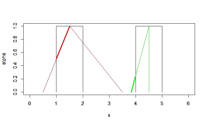
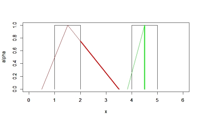
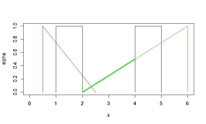
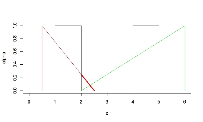
Figure 1: Representation of Example 4.4, part (i) in the top row and part (ii) in the bottom row. In each plot, the fuzzy sets $\mathcal{X}_{i}$ ($i=1,2$) are represented in black, $R$ in red and $G$ in green. Thick lines indicate the parts of $R$ and $G$ for which the corresponding support function is in the interval $[m_{\mathcal{X}}(u,\alpha),M_{\mathcal{X}}(u,\alpha)],$ with $u=-1$ in the left column and $u=1$ in the right column.

• Let $R,G\in\mathcal{F}_{c}(\mathbb{R}^{p})$ be defined, for any $t\in\mathbb{R},$ by

  $$R(t)\mathrel{\mathop{\mathchar 58\relax}}=(t-1/2)I_{[1/2,3/2]}(t)+(-t/2+7/4)I_{[3/2,7/2]}(t)$$

  $$G(t)\mathrel{\mathop{\mathchar 58\relax}}=(3t/2-23/4)I_{[23/6,9/2]}(t),$$

  Consequently, $R_{\alpha}=[\alpha+1/2,7/2-2\cdot\alpha]$ and $G_{\alpha}=[(2/3)\cdot\alpha+23/6,9/2],$ $\alpha\in[0,1],$ are their $\alpha$-levels and, for each $\alpha\in[0,1],$

  $$s_{R}(-1,\alpha)=-\alpha-1/2\mbox{, }s_{R}(1,\alpha)=7/2-2\cdot\alpha,$$

  $$s_{G}(-1,\alpha)=-(2/3)\cdot\alpha-23/6\mbox{ and }s_{G}(1,\alpha)=9/2$$

  are their support functions.

  To obtain the depth values, we first compute the Lebesgue measures of the $\alpha$’s for which these support functions belong to the intervals established in (17) and (18). We illustrate the computation with the top row of Figure 1. In the left plot, the thick red line is the part of the set $R$ for which $s_{R}(-1,\alpha)\in[-4,-1].$ This corresponds to $\alpha\in[.5,1]$ which results in a Lebesgue measure of 0.5. Meanwhile, in the right plot of Figure 1, the thick red line is the part of $R$ such that $s_{R}(1,\alpha)\in[2,5],$ which corresponds to $\alpha\in[0,.75],$ with Lebesgue measure .75. These measures add up to 5/4 with their minimum being 1/2.

  Analogously, the thick green line in the left plot is the part of set $G$ for which $s_{G}(-1,\alpha)\in[-4,-1].$ This corresponds to $\alpha\in[0,.25]$ which results in a Lebesgue measure of 0.25. In the right plot, the thick green line is the part of $G$ such that $s_{G}(1,\alpha)\in[2,5].$ It corresponds to $\alpha\in[0,1],$ which results in a Lebesgue measure 1. These measures add again up to 5/4 but this time their minimum is 1/4. Thus, making use of (17) and (18),

  $$D_{mS}(R;\mathcal{X})=D_{mS}(G;\mathcal{X})=5/8\mbox{ and }D_{FS}(R;\mathcal{X})=1/2\neq 1/4=D_{FS}(G;\mathcal{X}).$$

• Let $R,G\in\mathcal{F}_{c}(\mathbb{R}^{p})$ be defined, for any $t\in\mathbb{R},$ by

  $$R(t)\mathrel{\mathop{\mathchar 58\relax}}=(-t/2+5/4)I_{[1/2,5/2]}(t)$$

  $$G(t)\mathrel{\mathop{\mathchar 58\relax}}=(t/4-1/2)I_{[2,6]}(t).$$

  The corresponding $\alpha$-levels are $R_{\alpha}=[1/2,5/2-2\cdot\alpha]$ and $G_{\alpha}=[4\cdot\alpha+2,6],$ $\alpha\in[0,1]$. Thus, for each $\alpha\in[0,1],$ we have the support functions

  $$s_{R}(-1,\alpha)=-1/2\mbox{, }s_{R}(1,\alpha)=5/2-2\cdot\alpha\mbox{, }s_{G}(-1,\alpha)=-4\cdot\alpha-2\mbox{ and }s_{G}(1,\alpha)=6.$$

  As in the previous case, we compute the Lebesgue measures of the $\alpha$’s for which these support functions belong to the intervals established in (17) and (18). This time, we clarify the computation making use of the bottom row of Figure 1. As we can observe in the left plot, this time there is no thick red line, meaning that $s_{R}(-1,\alpha)\notin[-4,-1];$ and consequently the associated Lebesgue measure is 0. There is, however, a thick red line in the right plot, which coincides with the part of $R$ such that $s_{R}(1,\alpha)\in[2,5].$ This corresponds to $\alpha\in[0,.25],$ with a Lebesgue measure of .25. For $G,$ things are kind of opposed. $s_{G}(1,\alpha)\notin[2,5],$ which results in a 0 Lebesgue measure, and no thick green line in the bottom right plot of Figure 1. This time, for each $\alpha\in[0,.5]$ it is satisfied that $s_{G}(-1,\alpha)\in[-4,-1].$ This results in a larger thick green line in the bottom left plot that results in a Lebesgue measure of .5. Thus, for $R$ and $G$ the minimum Lebesgue measure is 0. Taking into account (13) and (14),

  $$D_{mS}(R;\mathcal{X})=1/8\neq 1/4=D_{mS}(G;\mathcal{X})\mbox{ and }D_{FS}(R;\mathcal{X})=0=D_{FS}(G;\mathcal{X}).$$

This example shows the relevant differences and similarities between $D_{mS}$ and $D_{FS}$. Let us comment them further, making use of the plots in Figure 1. Focussing on case (i), top row plots, we have that $R$ and $G$ take the same $D_{mS}$ depth value because the average of the amount of $\alpha$’s corresponding to the thick red lines between the two plots is the same as the average corresponding to the thick green lines. However, non of those amounts is the same, which is depicted by $D_{FS},$ providing different depth values. It gives smaller depth value to $G$ because the amount of $\alpha$’s corresponding to one of the thick green lines is the smallest among the four. In case (ii), bottom row plots, we have that $R$ and $G$ take the same $D_{FS}$ value because $R$ and $G$ result both in only one thick line each. $D_{mS}$ is able to depict a difference between $R$ and $G\mathrel{\mathop{\mathchar 58\relax}}$ that the thick line associated to $G$ is larger than that associated to $R;$ giving then a higher depth value to $G.$ As commented before, the difference is due to the distinct way in which they summarize the information. One can argue that $D_{mS}$ is potentially better because it uses more information by computing the average. On the other hand, it can also be argued that $D_{FS}$ will extract the relevant information in certain problems.

5 Properties of $D_{mS}$, $D_{FS}$, and $D_{nS}$

In this section, we will study whether the adaptations of simplicial depth to the fuzzy setting are semilinear and geometric depth functions in the sense of [8].

Theorem 5.2 collects properties of the simplicial depth functions $D_{mS}$ and $D_{FS}$. Its proof is based on proofs of the simplicial band depth [19, Theorems $1$ and $2$] and Proposition 5.1. The result is valid for $\mathcal{H}\subset C^{0}[\mathcal{F}_{c}(\mathbb{R}^{p})]$, namely fuzzy random variables all whose support functionals are continuous random variables. Note that, in order to define directly a notion of continuous fuzzy random variables, one would need first a reference measure with respect to which those variables would have a density function. In absence of such a measure (which would play the role of the Lebesgue measure in ${\mathbb{R}}^{p}$), the reduction to real random variables via the support function is more operative.

Proposition 5.1.

Let $\mathcal{X}\in L^{0}[\mathcal{F}_{c}(\mathbb{R}^{p})],$ $U\in\mathcal{F}_{c}(\mathbb{R}^{p})$ and $(u,\alpha)\in\mathbb{S}^{p-1}\times[0,1].$ Let $F_{u,\alpha}$ be the cumulative distribution function of the real random variable $s_{\mathcal{X}}(u,\alpha).$ Then

$$\mathbb{P}(s_{U}(u,\alpha)\in[m_{\mathcal{X}}(u,\alpha),M_{\mathcal{X}}(u,\alpha )])=1-[1-F_{u,\alpha}(s_{U}(u,\alpha))]^{p+1}$$

$$\hskip 28.45274pt-[F_{u,\alpha}(s_{U}(u,\alpha))-\mathbb{P}(s_{\mathcal{X}}(u,\alpha)=s_{U}(u,\alpha))]^{p+1}.$$

If, additionally, $\mathcal{X}\in C^{0}[\mathcal{F}_{c}(\mathbb{R}^{p})],$ that reduces to

$$\mathbb{P}(s_{U}(u,\alpha)\in[m_{\mathcal{X}}(u,\alpha),M_{\mathcal{X}}(u,\alpha)])=1-[1-F_{u,\alpha}(s_{U}(u,\alpha))]^{p+1}-[F_{u,\alpha}(s_{U}(u,\alpha))]^{p+1}.$$

Theorem 5.2.

When computed with respect to an $F$-symmetric random variable $\mathcal{X}\in C^{0}[\mathcal{F}_{c}(\mathbb{R}^{p})]$, $D_{mS}(\cdot;\mathcal{X})$ and $D_{FS}(\cdot;\mathcal{X})$ satisfy P1, P2, P3a and P3b for the $\rho_{r}$ distances for any $r\in(1,\infty)$.

In general, $D_{mS}$ and $D_{FS}$ violate P4a, as shown by the following example. They also violate P4b, since P4b implies P4a [8, Proposition $5.8$].

Example 5.3.

Let $(\{\omega_{1},\omega_{2}\},\mathcal{P}(\{\omega_{1},\omega_{2}\}),\mathbb{P})$ be a probability space such that $\mathbb{P}(\omega_{1})=\mathbb{P}(\omega_{2})$ and

$$\mathcal{X}\mathrel{\mathop{\mathchar 58\relax}}\{\omega_{1},\omega_{2}\}\rightarrow\mathcal{F}_{c}(\mathbb{R})\mbox{ with }\mathcal{X}(\omega_{1})=\text{I}_{\{1\}}\mbox{ and }\mathcal{X}(\omega_{2})=\text{I}_{\{-1\}}.$$

It is clear that $\mathcal{X}$ is $F$-symmetric with respect to $A=\text{I}_{\{0\}}$. Let $B\in\mathcal{F}_{c}(\mathbb{R})$ such that, for any $t\in\mathbb{R},$

$$B(t)\mathrel{\mathop{\mathchar 58\relax}}=(-t/2+1/2)I_{(0,1]}(t)+I_{\{0\}}(t).$$

Thus, we have that

$$B_{\alpha}=[0,1-2\alpha]\mbox{ for }\alpha\in[0,1/2]\mbox{ and }B_{\alpha}=\{0\}\mbox{ for any }\alpha\in[1/2,1].$$

Additionally,

$$s_{B}(-1,\alpha)=0\mbox{ for all }\alpha\in[0,1]\mbox{ and }s_{B}(1,\alpha)=0\mbox{ for all }\alpha\in[1/2,1].$$

Taking into account the definition of $D_{FS}$, we have that, for all $n\in\mathbb{N},$

$$D_{FS}(A+n\cdot B;\mathcal{X})\geq 1/2;\mbox{ consequently, }\lim_{n\rightarrow\infty}D_{FS}(A+n\cdot B;\mathcal{X})>0.$$

Analogously, we have that $D_{mS}(A+n\cdot B;\mathcal{X})\geq 1/2$ for all $n\in\mathbb{N}$, thus

$$\lim_{n\rightarrow\infty}D_{mS}(A+n\cdot B;\mathcal{X})>0.$$

In property P4a we study sequences of fuzzy sets of the form $\{A+n\cdot B\}_{n}$. By restricting the selection of the fuzzy set $B$ to the family of fuzzy sets satisfies P4a

$$\mathfrak{B}\mathrel{\mathop{\mathchar 58\relax}}=\{B\in\mathcal{F}_{c}(\mathbb{R}^{p})\mathrel{\mathop{\mathchar 58\relax}}\forall u\in\mathbb{S}^{p-1}, \exists C_{u}\subseteq[0,1]\mbox{ with }\nu(C_{u})=1$$

$$\mbox{ such that }s_{B}(u,\alpha)\neq 0\mbox{ }\forall\alpha\in C_{u}\},$$

the following result holds for $D_{FS}$ and $D_{mS},$ which is in line with property P4a. Property P4b, however, considers a general sequence of fuzzy sets $\{A_{n}\}_{n},$ not allowing for this type of adaptation.

Proposition 5.4.

For any $\mathcal{X}\in L^{0}[\mathcal{F}_{c}(\mathbb{R}^{p})]$ and $B\in\mathfrak{B},$ we have that

• $\lim_{n}D_{FS}(A+n\cdot B;\mathcal{X})=0,$ with $A\in\mathcal{F}_{c}(\mathbb{R}^{p})$ maximizing $D_{FS}(\cdot;\mathcal{X}).$

• $\lim_{n}D_{mS}(A+n\cdot B;\mathcal{X})=0,$ with $A\in\mathcal{F}_{c}(\mathbb{R}^{p})$ maximizing $D_{mS}(\cdot;\mathcal{X}).$

The following result is for $D_{nS}$.

Theorem 5.5.

For any $\mathcal{X}\in L^{0}[\mathcal{F}_{c}(\mathbb{R}^{p})],$ $D_{nS}(\cdot;\mathcal{X})$ satisfies P1, P4a and P4b for the $d_{r}$ distances for any $r\in[1,\infty]$ and for the $\rho_{r}$ distances for any $r\in[1,\infty).$

For property P2, intuitively, the notion of symmetry to be considered would make use of the central symmetry of the support function of a fuzzy set in every $u\in\mathbb{S}^{p-1}$ and $\alpha\in[0,1]$. It is apparent that the relation between this tentative notion of symmetry and the notion of a fuzzy simplex is $F$-symmetry. As regards properties P3a and P3b, already in the multivariate case the simplicial depth does not generally satisfy the analog property M3. Because of these reasons and since naive simplicial fuzzy depth is not one of our recommended fuzzy depth, we do not pursue these properties further.

6 Empirical simplicial depths

Given $\mathcal{H}\subseteq L^{0}[\mathcal{F}_{c}(\mathbb{R}^{p})],$ let $\mathcal{X}\in\mathcal{H}$ be a fuzzy random variable and $\mathcal{X}_{1},\ldots,\mathcal{X}_{n}$ be independent random variables distributed as $\mathcal{X}.$ Let $\mathfrak{X}$ be a fuzzy random variable corresponding to the empirical distribution associated to $\mathcal{X}_{1},\ldots,\mathcal{X}_{n}$. That is, $\mathfrak{X}$ takes on as values the observed values $\mathcal{X}_{1}(\omega),\ldots,\mathcal{X}_{n}(\omega)$ (possibly repeated) with probability $n^{-1}$. The simplicial depths associated with this empirical distribution are the empirical or sample simplicial depths.

In Subsection 6.1, we provide the explicit definitions for the case of $\mathcal{F}_{c}(\mathbb{R})$ in order to illustrate subsequently the behavior of our three proposals. For ease of comparison with Tukey depth, we use in Subsection 6.3 the same dataset in [8]. The behaviour is similar, which is interesting since that distribution is not from $C^{0}[\mathcal{F}_{c}(\mathbb{R}^{p})]$ as assumed by some of our theoretical results (Theorem 5.2). In order to illustrate the case of fuzzy random variables with continuously distributed support functionals, we generate in Section 6.2 a synthetic sample from a fuzzy random variable in $C^{0}[\mathcal{F}_{c}(\mathbb{R}^{p})]$.

6.1 Empirical definitions for $\mathcal{F}_{c}(\mathbb{R})$

From (13) and (14), $D_{mS}$ and $D_{FS}$ have in common that both involve computing the function

$$F_{A}(u)\mathrel{\mathop{\mathchar 58\relax}}=\int_{[0,1]}\mathbb{P}(s_{A}(u,\alpha)\in[m_{\mathcal{X}}(u,\alpha),M_{\mathcal{X}}(u,\alpha)])\operatorname{d\!}\nu(\alpha),$$

with $u\in\mathbb{S}^{0}=\{-1,1\}.$ The difference lies in the operator over $\mathbb{S}^{0}$ applied to $F_{A}\mathrel{\mathop{\mathchar 58\relax}}$ the average (for $D_{mS}$) and the infimum (for $D_{FS}$). Then, to establish our proposals of emprirical simplicial and modified simplicial fuzzy depth, making use of $\mathcal{X}_{1},\ldots,\mathcal{X}_{n},$ we calculate $F_{A}(u)$ for the fuzzy random variable $\mathfrak{X}$ as $\binom{n}{2}^{-1}L^{A}_{n}(u)$ with

$$L^{A}_{n}(u)\mathrel{\mathop{\mathchar 58\relax}}=\sum_{i=1}^{n}\sum_{j\geq i}^{n}L_{i,j,u}^{A}$$ (19)

and

$$L_{i,j,u}^{A}\mathrel{\mathop{\mathchar 58\relax}}=\nu(\{\alpha\in[0,1]\mathrel{\mathop{\mathchar 58\relax}}s_{A}(u,\alpha)\in[\min\{s_{\mathcal{X}_{i}}(u,\alpha),s_{\mathcal{X}_{j}}(u,\alpha)\},\max\{s_{\mathcal{X}_{i}}(u,\alpha),s_{\mathcal{X}_{j}}(u,\alpha)\}]\}).$$ (20)

Then, the modified simplicial fuzzy depth based on $\mathcal{J}\subseteq\mathcal{F}_{c}(\mathbb{R})$ of a fuzzy set $A\in\mathcal{J}$ with respect to $\mathfrak{X}$ is

$$D_{mS}(A;\mathfrak{X})=\int_{\mathbb{S}^{0}}\binom{n}{2}^{-1}L_{n}^{A}(u)\operatorname{d\!}\mathcal{V}_{1}(u)=2^{-1}\binom{n}{2}^{-1}\left[L_{n}^{A}(1)+L_{n}^{A}(-1)\right]$$ (21)

and the simplicial fuzzy depth based on $\mathcal{J}\subseteq\mathcal{F}_{c}(\mathbb{R})$ of a fuzzy set $A\in\mathcal{J}$ with respect to $\mathfrak{X}$ is

$$D_{FS}(A;\mathfrak{X})=\inf_{u\in\mathbb{S}^{0}}\binom{n}{2}^{-1}L_{n}^{A}(u)=\binom{n}{2}^{-1}\min\{L_{n}^{A}(1),L_{n}^{A}(-1)\}.$$ (22)

Similarly, the naive simplicial fuzzy depth based on $\mathcal{J}\subseteq\mathcal{F}_{c}(\mathbb{R})$ of a fuzzy set $A\in\mathcal{J}$ with respect to $\mathfrak{X}$ is

$$D_{nS}(A;\mathfrak{X})=\cfrac{1}{\binom{n}{2}}\sum_{i=1}^{n}\sum_{j\geq i}^{n}I_{i,j}^{A},$$ (23)

where $I_{i,j}^{A}$ equals 1 if $s_{A}(u,\alpha)\in[\min\{s_{\mathcal{X}_{i}}(u,\alpha),s_{\mathcal{X}_{j}}(u,\alpha)\},\max\{s_{\mathcal{X}_{i}}(u,\alpha),s_{\mathcal{X}_{j}}(u,\alpha\}]$ for every $(u,\alpha)\in\mathbb{S}^{0}\times[0,1]$, and 0 otherwise.

6.2 Simulated data

We draw a sample ($n=100$) from a fuzzy random variable in $C^{0}[\mathcal{F}_{c}(\mathbb{R}^{p})]$. For that, we make use of a random variable whose realizations are trapezoidal fuzzy sets. To construct the fuzzy random variable, we follow the method in [30]. Let $X_{1},X_{2},X_{3},X_{4}$ be independent and continuous real-valued random variables. Let $X_{1}$ be normally distributed with zero mean and standard deviation 10, whereas $X_{2},X_{3},X_{4}$ are chi-squared distributions with 1 degree of freedom. Set

$$\mathcal{X}=\mbox{Tra}(X_{1}-X_{2}-X_{3},X_{1}-X_{2},X_{1}+X_{2},X_{1}+X_{2}+X_{4})$$ (24)

which is well-defined since $X_{2},X_{3},X_{4}\geq 0$. By construction,

$$s_{\mathcal{X}}(-1,\alpha)=-(X_{1}-X_{2}-(1-\alpha)X_{3})$$

and

$$s_{\mathcal{X}}(1,\alpha)=X_{1}+X_{2}+(1-\alpha)X_{4},$$

which are continuous variables for each $\alpha\in[0,1]$. Accordingly, $\mathcal{X}\in C^{0}[\mathcal{F}_{c}(\mathbb{R})]$ as required by Theorem 5.2.

The choice of the $\chi_{1}^{2}$ distribution for $X_{3},X_{4}$ is because it is very skewed (Pearson coefficient: $2\sqrt{2}$). That allows us to realize how the depth is affected not just by the location of the core of the trapezoidal fuzzy set but also by the slopes of its sides.

To illustrate the performance of the different depth functions, let $\mathcal{X}_{1},\ldots,\mathcal{X}_{100}$ be independent copies distributed as $\mathcal{X}.$ With some abuse of notation, for $i=1,\ldots,100,$ each $\mathcal{X}_{i}$ will also denote the observed trapezoidal fuzzy set, represented in each of the plots of Figure 2. Thus, we illustrate the performance of each of our three proposals by computing, for $i=1,\ldots,100,$ each of the depths of $\mathcal{X}_{i}$ with respect to the corresponding empirical fuzzy random variable $\mathfrak{X}.$ Naive simplicial depth $D_{nS}$ is illustrated in the top row of Figure 2, modified simplicial depth $D_{mS}$ in the middle row, and simplicial fuzzy depth $D_{FS}$ in the bottom row. The plots in the first column of Figure 2 represent the five trapezoidal fuzzy values having the largest depth values. These are colored from red (highest depth) to yellow (high depth) and the rest of the 100 in grey. A zoom of each of these plots highlighting the deepest sets is in the central column of the figure.

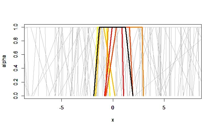
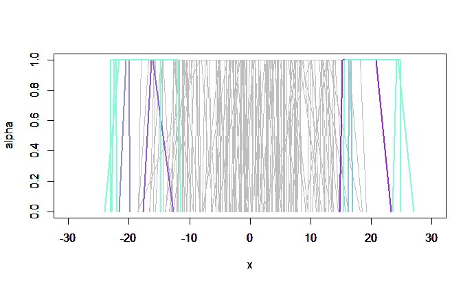
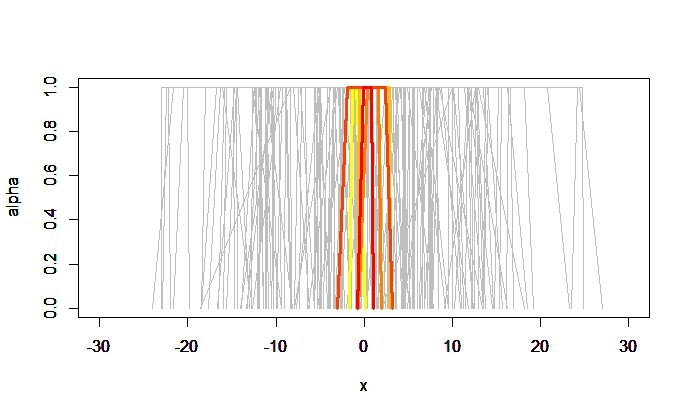
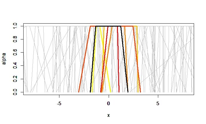
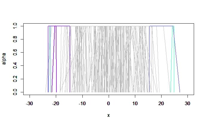
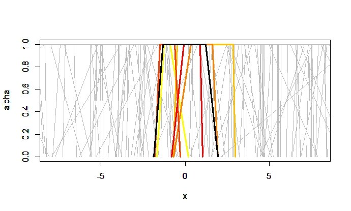
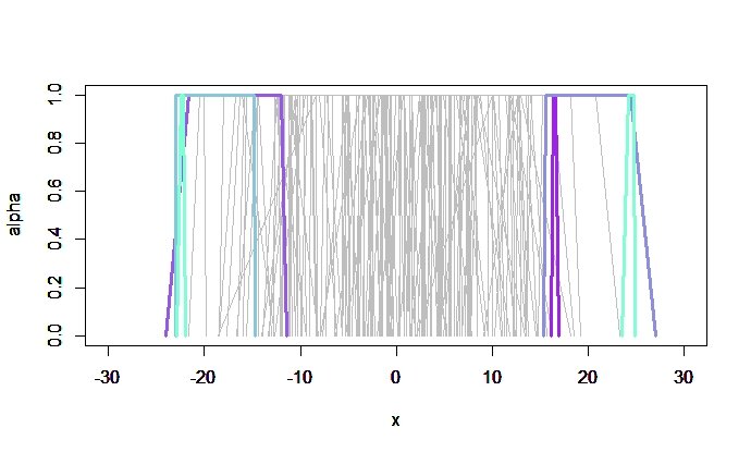
Figure 2: Illustration of the empirical naive simplicial fuzzy depth, $D_{nS},$ (top row), the empirical modified simplicial fuzzy depth, $D_{mS},$ (middle row) and the empirical simplicial fuzzy depth, $D_{FS,}$ (bottom row) over a sample of trapezoidal fuzzy sets of size 100 drawn from $\mathcal{X}$ in (24). The sample is plotted in grey. The color in the first and second column plots represent the trapezoidal fuzzy sets in the sample corresponding to the 5 larger depth values, with the second column being a zoom of the first in the interval $[-8,8];$ in order to better observe the different depth values. Colors range from red (highest depth) to yellow (high depth) in the first column. In addition, in the second column the median fuzzy set is highlighted in black. The third column represents the trapezoidal fuzzy sets with the 5 minimal depth values for the same depth functions. Depth values are shown through the colors, which range from aqua marine blue (lowest depth) to violet (low depth).

We also represent, plotted in black in the central column of Figure 2, the median fuzzy set, $M$, with respect to the sample $\mathcal{X}_{1},\ldots,\mathcal{X}_{100}$. Denoting $\mathcal{X}_{i}=\text{Tra}(a_{i},b_{i},c_{i},d_{i})$ for every $i\in\{1,\ldots,100\}$, the median fuzzy set is defined as

$$M\mathrel{\mathop{\mathchar 58\relax}}=\text{Tra}(\text{Med}(a_{1},\ldots,a_{100}),\text{Med}(b_{1},\ldots,b_{100}),\text{Med}(c_{1},\ldots,c_{100}),\text{Med}(d_{1},\ldots,d_{100})).$$

This coincides with the definition in [30]. The median $M$ is not necessarily one of the sample fuzzy sets; and in the particular case of Figure 2, it is not. The maximizers of the depth functions $D_{nS}$, $D_{mS}$ and $D_{FS}$ provide alternative definitions of a median fuzzy set. They are in the vicinity of $M$ (represented in yellow in the figure) but they are not identical with $M$.

The right column of Figure 2 shows the trapezoidal fuzzy sets with the minimal 5 depth values for the three different proposals of simplicial depth. The trapezoidal fuzzy sets with minimal depth are the ones furthest to the left and right, as expected. It is observable from the plots that the three definitions order the sets with minimal depth in a similar way. The main difference lies in that $D_{nS}$ gives a high number of ties (observe how many sets are colored in aquamarine blue in the last column of the first row). The reason for this is that $D_{nS}$ is a sum of indicator functions (23) while the other two proposals make use the Lebesgue measure [(20), (21) and (22)]. Thus, it is generally more convenient to use the proposals $D_{mS}$ and $D_{FS}$ instead of $D_{nS};$ with results for $D_{nS}$ being inappropriate for some applications like classification. The use of a sum of indicator functions versus the Lebesgue measure also explains that $D_{nS}$ results in smaller depth values than $D_{mS}$ or $D_{FS}.$

The main difference between $D_{mS}$ and $D_{FS},$ of a fuzzy set $A\in\mathcal{F}_{c}({\mathbb{R}}^{p}),$ is that the first one takes the average of $L^{A}_{n}(u)$ in (19) between $u=-1$ and $u=1$ and the second one its minimum over $u\in\{1,-1\}$. Thus, a fuzzy number $A$ with, for instance,

$$L^{A}_{n}(1)\mbox{ close to }L^{M}_{n}(1)\mbox{ and }L^{A}_{n}(-1)\mbox{ far from }L^{M}_{n}(-1)$$

does not take a maximal depth value with $D_{FS}$ but can take it with $D_{mS}.$ This is observed in the central column of Figure 2.

A similar phenomenon is observed with the fuzzy numbers taking minimal depth values. The bottom row right column plot in Figure 2 shows that there exists fuzzy numbers in the sample with minimal depth for $D_{FS},$ some are on the left side of the plot and the others on the right side. Among the ones on the left there are those that have, for instance,

$$L^{A}_{n}(-1)\mbox{ far from }L^{M}_{n}(-1)\mbox{ while }L^{A}_{n}(1)\mbox{ is not as far from }L^{M}_{n}(1).$$

Analogously, among the ones on the right there those that have, for instance,

$$L^{A}_{n}(1)\mbox{ far from }L^{M}_{n}(1)\mbox{ while }L^{A}_{n}(-1)\mbox{ is not as far from }L^{M}_{n}(-1).$$

As it observable from the central row right column plot in Figure 2, these fuzzy numbers does not necessarily take minimal depth value with $D_{mS},$ as this depth function takes the average between $L^{A}_{n}(1)$ and $L^{A}_{n}(-1)$.

6.3 Real data

We use the Trees dataset (from the SAFD R package for Statistical Analysis of Fuzzy Data), which was first used in [4]. This comes from a reforestation project in the region of Asturias (Northern Spain) by the INDUROT forest institute at the University of Oviedo. The project takes into account three species of trees: birch (Betula celtiberica), sessile oak (Quercus petraea) and rowan (Sorbus aucuparia).

The most important variable considered is the quality of trees, whose observations are trapezoidal fuzzy sets coming from an expert subjective assessment of height, diameter, leaf structure and other features. The dataset is represented in Figure 3, where quality is measured in the x-axis in the range 1–5, from low to perfect quality. The membership values for each trapezoidal fuzzy set are represented in the y-axis.

The dataset is comprised of 9 different trapezoidal fuzzy values, represented in Figure 3. Therefore, the assumption in our theoretical study that each support functions has a continuous distribution is violated, which makes it interesting to check the depth functions’ behavior. From left to right we denote them by $T_{1},\ldots,T_{9}.$ These sets appear in the sample with a certain multiplicity, resulting in a sample $\mathcal{X}_{1},\ldots,\mathcal{X}_{n}$ of size $n=279.$ Table 1 shows the absolute frequency of the fuzzy sets in the sample. We denote by $\mathfrak{X}$ the fuzzy random variable corresponding to the empirical distribution associated to $\mathcal{X}_{1},\ldots,\mathcal{X}_{n}.$

$T_{1}$	$T_{2}$	$T_{3}$	$T_{4}$	$T_{5}$	$T_{6}$	$T_{7}$	$T_{8}$	$T_{9}$
22	16	39	36	85	22	35	12	12

Table 1: Number of sets in the sample for each type of trapezoidal fuzzy set. Absolute frequency of each distinct trapezoidal fuzzy set $T_{i},$ $i=1,\ldots,9,$ represented in Figure 3.

One can observe from Figure 3 that

$$s_{T_{i}}(1,\alpha)\geq s_{T_{j}}(1,\alpha)\mbox{ and }s_{T_{i}}(-1,\alpha)\leq s_{T_{j}}(-1,\alpha)$$ (25)

for each $\alpha\in[0,1]$ and $i,j\in\{1,\ldots 9\}$ with $i\leq j$. In fact the inequalities are strict except for the cases of $T_{4},T_{5}$ and $T_{6}$, where

$$s_{T_{4}}(-1,0)=s_{T_{5}}(-1,0)\mbox{ and }s_{T_{5}}(1,0)=s_{T_{6}}(1,0).$$ (26)

Taking into account the sample version of $D_{nS}$ in (23) and the fact that $I_{i,j}^{A}$ takes value $1$ if

$$s_{A}(u,\alpha)\in[\min\{s_{\mathcal{X}_{i}}(u,\alpha),s_{\mathcal{X}_{j}}(u,\alpha)\},\max\{s_{\mathcal{X}_{i}}(u,\alpha),s_{\mathcal{X}_{j}}(u,\alpha)\}]$$

for every $(u,\alpha)\in\mathbb{S}^{0}\times[0,1]$ and $0$ otherwise, the computation of $D_{nS}(T_{i};\mathfrak{X})$ reduces to computing the simplicial depth in $\mathbb{R}$ of $s_{T_{i}}(u,\alpha)$ with respect to $s_{\mathfrak{X}}(u,\alpha)$ for some $(u,\alpha)$ where the inequalities in (25) are strict. Taking into account (26), this is the case of $(u,\alpha)=(1,1),$ for instance. Thus

$$D_{nS}(T_{i};\mathfrak{X})=SD(s_{T_{i}}(1,1);s_{\mathfrak{X}}(1,1))$$

for each $i\in\{1,\ldots,9\}$.

Taking into account the order given by (25) of $\{T_{i}\}_{i=1}^{9}$ for each $(u,\alpha)\in\mathbb{S}^{0}\times[0,1]$ and $i\leq j$ with $i,j\in\{1,\ldots 9\},$ we have that $L_{i,j,u}^{T_{k}}=1$ for each $k\in[i,j]$ and $0$ otherwise. Considering the sample versions of $D_{mS}$ and $D_{FS}$ in (21) and (22), we have that in this case the three depth proposals coincide, that is,

$$D_{nS}(T_{i};\mathfrak{X})=D_{mS}(T_{i};\mathfrak{X})=D_{FS}(T_{i};\mathfrak{X})$$

for each $i\in\{1,\ldots,9\}$. Thus, in computing the depth of an element in the dataset with respect to the empirical fuzzy random variable, we obtain the same depth value independently of which of the three simplicial based fuzzy depths is used. The left plot of Figure 3 represents in the color the depth values of each of the 9 distinct trapezoidal elements in the dataset. Colors range from brown (high depth) to yellow (low depth).

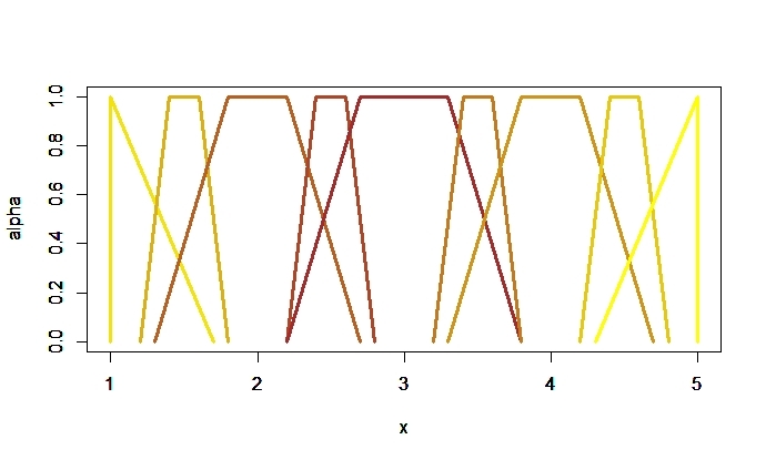
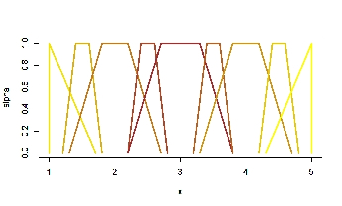
Figure 3: Display of the fuzzy sets in the Trees dataset. In the first column, color is assigned based on the Simplicial depth of each fuzzy set in the empirical distribution. Colors range from brown (high depth) to yellow (low depth). The second column applies the same procedure but considering the Tukey depth.

From Figure 3 we can observe that the order induced in the dataset by the simplicial and Tukey fuzzy depth functions is similar. In fact, the only difference is $T_{3}$ and $T_{6}.$ In the case of the simplicial fuzzy depths, we have that $T_{3}$ is the third deepest set and $T_{6}$ is the fourth, while we obtain the reverse using the Tukey fuzzy depth. Let us explain where this difference comes from. If we observe Table 1 we have that $T_{3}$ has 39 repetitions in the sample while $T_{6}$ only has 22. On the other hand the diameter of 0-level and the 1-level of $T_{3}$ is greater than the diameter of the 0-level and the 1-level of $T_{6}$. Thus, taking into account that the weight of $T_{3}$ in the sample is greater than the weight of $T_{6},$ as the Tukey depth is defined as a minimum, it could be an explanation of why

$$D_{FT}(T_{6};\mathcal{X})>D_{FT}(T_{3};\mathcal{X}).$$

Meanwhile, as the simplicial depth for fuzzy sets is defined by an integral, it takes more into account the weights of the different sets of the sample and depreciates what happens in one single point.

7 Discussion

Simplicial depth is one of the most widely used depth functions in multivariate statistics. It is built over the notion of simplex in $\mathbb{R}^{p}$. In the space of fuzzy sets, the notion of simplex is not an obvious one. With the characterization introduced in Proposition 3.1 of simplices in the multivariate space, we justify the notion of simplex in $\mathcal{K}_{c}(\mathbb{R}^{p})$ and extend it to the fuzzy setting, working $\alpha$-level by $\alpha$-level (Definition 3.5). Making use of this notion, we propose a straightforward definition of simplicial depth for the fuzzy setting and two elaborate and sounded definitions.

• The naive simplicial fuzzy depth (9), $D_{nS}$, is equivalent to the multivariate simplicial depth. We prove some properties for it in Theorem 5.5 and show it may result in a high number of ties at zero, which is not desirable for instance in classification problems.

• The modified simplicial fuzzy depth (Definition 4.2), $D_{mS},$ improves the naive simplicial fuzzy depth analogously to how the modified band depth improves the band depth; resulting in less zero depth values.

• The simplicial fuzzy depth (Definition 4.3), $D_{FS}$, transforms the modified simplicial fuzzy depth in the direction of the Tukey depth; doing so by applying the infimum over $\mathbb{S}^{p-1}$ instead of the expected value.

Although it is clear throughout the paper the authoritativeness of $D_{mS}$ and $D_{FS}$ over $D_{nS},$ there is not a clear winner between $D_{mS}$ and $D_{FS}.$ The practical similarities and differences between them are discussed in Example 4.4 and Subsection 6.2. Their properties are collected in Theorem 5.2 and Proposition 5.4. For some of these properties it is required fuzzy random variables to satisfy certain type of continuity. This is inherited from the fact that the multivariate simplicial depth requires of continuous distributions to satisfy the notion of multivariate depth.

Our three proposals neither satisfy the notion of semilinear nor of geometric depth function in [8] because of the lack of satisfaction of the entirety of the properties constituting these notions (Section 5). However, as we can see in the illustrations in Section 6, the behavior of the three proposals is similar in practice. As shown there, it is also similar to that of the Tukey fuzzy depth, despite Tukey does satisfy both notions and the comparison is done with respect to a fuzzy random variable that does not satisfy the continuity properties required in Theorem 5.2.

For future work, it is interesting to study more instances of fuzzy depth, creating a library of depth functions for the fuzzy setting. Also, we consider it is compelling to study more properties for the Tukey fuzzy depth and the simplicial fuzzy depths, such as convergence of the sample depth to the population depth (consistency) and their continuity or semicontinuity properties.

8 Proofs

Proof of Proposition 3.1.

Let us denote

$$\mathcal{C}\mathrel{\mathop{\mathchar 58\relax}}=\{x\in\mathbb{R}^{p}\mathrel{\mathop{\mathchar 58\relax}}\langle u,x\rangle\in[m(u),M(u)]\text{ for all }u\in\mathbb{S}^{p-1}\}.$$

First, we prove $S[x_{1},\ldots,x_{p+1}]\subseteq\mathcal{C}$. Let $x\in S[x_{1},\ldots,x_{p+1}]$. By (5), there exists $\lambda_{1},\ldots,\lambda_{p+1}\geq 0$ with $\sum_{i=1}^{p+1}\lambda_{i}=1$ such that $x=\sum_{i=1}^{p+1}\lambda_{i}x_{i}.$ For any fixed direction $u\in\mathbb{S}^{p-1}$, we have $\langle u,x\rangle=\sum_{i=1}^{p+1}\lambda_{i}\langle u,x_{i}\rangle.$ As $\lambda_{i}\in[0,1]$ for all $i=1,\ldots,p+1,$ we have that $\langle u,x\rangle\in[m(u),M(u)];$ and, consequently, $x\in\mathcal{C}$.

Now, let $x\in\mathcal{C}$ and suppose for a contradiction that $x\not\in S[x_{1},\ldots,x_{p+1}]$. The simplex $S[x_{1},\ldots,x_{p+1}]$ and the set $\{x\}$ are closed, convex and bounded subsets of $\mathbb{R}^{p}$. By the Hyperplane Separation Theorem (see, e.g., [26]), there exist $u\in\mathbb{R}^{p}$ and $b\in\mathbb{R}$ such that $\langle u,x\rangle>b$ and $\langle u,s\rangle<b$ for all $s\in S[x_{1},\ldots,x_{p+1}]$. This implies that $\langle u,x\rangle>\langle u,s\rangle$ for all $s\in S[x_{1},\ldots,x_{p+1}]$. Normalizing the vector $u$, $\bar{u}\in S^{p-1}$, we have that $\langle\bar{u},x\rangle>M(\bar{u}).$ This is a contradiction with the fact that $x\in\mathcal{C}$. Thus, $x\in S[x_{1},\ldots,x_{p+1}].$ ∎

Proof of Proposition 3.3.

Let $A_{1},\ldots,A_{p+1}\in\mathcal{K}_{c}(\mathbb{R}^{p})$ and $A\in\mathcal{K}_{c}(\mathbb{R}^{p})$ such that there exist real numbers $\lambda_{1},\ldots,\lambda_{p+1}\geq 0$ with $\sum_{i=1}^{p+1}\lambda_{i}=1$ and $A=\sum_{i=1}^{p+1}\lambda_{i}\cdot A_{i}$. By (2), $s_{A}(u)=\sum_{i=1}^{p+1}\lambda_{i}\cdot s_{A_{i}}(u)$ for every $u\in\mathbb{S}^{p-1}$. Thus, for every $u\in\mathbb{S}^{p-1},$

$$m(u)=(\sum_{i=1}^{p+1}\lambda_{i})m(u)\leq s_{A}(u)\leq(\sum_{i=1}^{p+1}\lambda_{i})M(u)=M(u).$$

Then $A\in S_{c}[A_{1},\ldots,A_{p+1}]$. ∎

Proof of Proposition 3.8.

For any $A\in{\mathcal{F}_{c}}({\mathbb{R}})$, since $\mathbb{S}^{0}=\{-1,1\}$ we have

$$s_{A}(1,\alpha)=\sup A_{\alpha},\quad s_{A}(-1,\alpha)=\sup\{-x\mid x\in A_{\alpha}\}=-\inf A_{\alpha}.$$

For any fixed $\alpha$, inequality $m(u\alpha)\leq s_{A}(u,\alpha)\leq M(u\alpha)$ will hold for $u=1$ if and only if

$$\min\{\sup(A_{1})_{\alpha},\sup(A_{2})_{\alpha}\}\leq\sup A_{\alpha}\leq\max\{\sup(A_{1})_{\alpha},\sup(A_{2})_{\alpha}\}$$

which, taking into account the assumption $A_{1}\preceq A_{2}$, is equivalent to

$$\sup(A_{1})_{\alpha}\leq\sup A_{\alpha}\leq\sup(A_{2})_{\alpha}.$$

In its turn, the inequality will hold for $u=-1$ if and only if

$$\min\{-\inf(A_{1})_{\alpha},-\inf(A_{2})_{\alpha}\}\leq-\inf A_{\alpha}\leq\max\{-\inf(A_{1})_{\alpha},-\inf(A_{2})_{\alpha}\}$$

or, multiplying all terms by $-1$,

$$\max\{\inf(A_{1})_{\alpha},\inf(A_{2})_{\alpha}\}\geq\inf A_{\alpha}\geq\min\{\inf(A_{1})_{\alpha},\inf(A_{2})_{\alpha}\}$$

which, again by the assumption $A_{1}\preceq A_{2}$, is the same thing as

$$\inf(A_{2})_{\alpha}\geq\inf A_{\alpha}\geq\inf(A_{1})_{\alpha}.$$

The conjunction of those two conditions is just $A_{1}\preceq A\preceq A_{2}$. Hence

$$S_{F}[A_{1},A_{2}]=\{A\in{\mathcal{F}_{c}}({\mathbb{R}}^{d})\mathrel{\mathop{\mathchar 58\relax}}A_{1}\preceq A\preceq A_{2}\}.$$

∎

Proof that the naive simplicial fuzzy depth is well defined.

We need to show that the event

$$\{s_{A}(u,\alpha)\in[m_{\mathcal{X}}(u,\alpha),M_{\mathcal{X}}(u,\alpha)]\mbox{ for all }(u,\alpha)\in\mathbb{S}^{p-1}\times[0,1]\}$$

$$=\bigcap_{u\in\mathbb{S}^{p-1}}\bigcap_{\alpha\in[0,1]}\{s_{A}(u,\alpha)\in[m_{\mathcal{X}}(u,\alpha),M_{\mathcal{X}}(u,\alpha)]\}$$

is measurable.

First, for each fixed $u,\alpha$ and $i=1,\ldots,p-1$, the mapping $s_{\mathcal{X}_{i}}(u,\alpha)$ is a random variable [12, Lemma 4]. Subsequently,

$$\Omega_{u,\alpha}\mathrel{\mathop{\mathchar 58\relax}}=\{s_{A}(u,\alpha)\in[m_{\mathcal{X}}(u,\alpha),M_{\mathcal{X}}(u,\alpha)]\}$$

$$=\left(\bigcup_{i=1}^{p+1}\{s_{\mathcal{X}_{i}}(u,\alpha)\leq s_{A}(u,\alpha)\}\right)\cap\left(\bigcup_{i=1}^{p+1}\{s_{\mathcal{X}_{i}}(u,\alpha)\geq s_{A}(u,\alpha)\}\right)$$

is measurable.

Taking $D$ a countable dense subset of $[0,1]$ such that $0\in D,$ let us prove

$$\bigcap_{\alpha\in[0,1]}\Omega_{u,\alpha}=\bigcap_{\alpha\in D}\Omega_{u,\alpha}\quad\hbox{ for each fixed }u\in\mathbb{S}^{p-1}.$$ (27)

The left-to-right inclusion is trivial. For the converse inclusion, assume for now that $\alpha\in(0,1]$. We can construct a sequence of elements of $D$ converging to $\alpha$ from the left (which is why $\alpha>0$ is needed). Indeed, for each $n\in{\mathbb{N}}$ with $n>\alpha^{-1}$ consider the open interval $(\alpha-n^{-1},\alpha)$. It contains some $\alpha_{n}\in D,$ because of $D$ being dense. Since $\alpha-n^{-1}<\alpha_{n}<\alpha$, we have $\alpha_{n}\to\alpha^{-}$. Now the mapping $s_{A}(u,\cdot)$ is left continuous [20]. Similarly, for any arbitrary $\omega\in\Omega$, the $s_{\mathcal{X}_{i}(\omega)}(u,\cdot)$ are left continuous, whence $m(u,\cdot)$ and $M(u,\cdot)$ are too. For any $\omega\in\bigcap_{\alpha\in D}\Omega_{u,\alpha}$ we have

$$m(u,\alpha_{n})\leq s_{A}(u,\alpha_{n})\leq M(u,\alpha_{n})$$

(please note the unspecified dependence of $m$ and $M$ on $\omega$ via the $s_{\mathcal{X}_{i}}$). By the left continuity, also

$$m_{\mathcal{X}}(u,\alpha)\leq s_{A}(u,\alpha)\leq M_{\mathcal{X}}(u,\alpha).$$

This means that $\omega$ is in $\Omega_{u,\alpha}$ for each $\alpha\in(0,1]$. The case $\alpha=0$ holds as well since we chose $D$ with $0\in D$. Accordingly, (27) holds. That proves that each $\bigcap_{\alpha\in[0,1]}\Omega_{u,\alpha}$, being a countable intersection of measurable events, is measurable.

$\mathbb{S}^{p-1}$, being a compact metric space, is separable. Let us take a countable dense subset $D^{\prime}\subseteq\mathbb{S}^{p-1}$. The proof will be complete if we show

$$\bigcap_{u\in\mathbb{S}^{p-1}}\bigcap_{\alpha\in[0,1]}\Omega_{u,\alpha}=\bigcap_{u\in D^{\prime}}\bigcap_{\alpha\in[0,1]}\Omega_{u,\alpha},$$

since the left-hand side is the event we wish to prove measurable and the right-hand side is a countable intersection of measurable events. As before, only the right-to-left inclusion need be proved. Let us fix an arbitrary $u^{*}\in\mathbb{S}^{p-1}$. Due to $D^{\prime}$ being dense, there exists a sequence $u_{n}\to u^{*}$ with $u_{n}\in D^{\prime}$. Whenever $\omega\in\bigcap_{u\in D^{\prime}}\bigcap_{\alpha\in[0,1]}\Omega_{u,\alpha}$, we have

$$m(u_{n},\alpha)\leq s_{A}(u_{n},\alpha)\leq M(u_{n},\alpha)\hbox{ for all }\alpha\in[0,1].$$

By the continuity of the support functions for fixed $\alpha$ [20], the convergence $u_{n}\to u^{*}$ implies

$$m(u^{*},\alpha)\leq s_{A}(u^{*},\alpha)\leq M(u^{*},\alpha)\hbox{ for all }\alpha\in[0,1].$$

That establishes

$$\bigcap_{u\in D^{\prime}}\bigcap_{\alpha\in[0,1]}\Omega_{u,\alpha}\subseteq\bigcap_{\alpha\in[0,1]}\Omega_{u^{*},\alpha}.$$

By the arbitrariness of $u^{*}$,

$$\bigcap_{u\in D^{\prime}}\bigcap_{\alpha\in[0,1]}\Omega_{u,\alpha}\subseteq\bigcap_{u\in\mathbb{S}^{p-1}}\bigcap_{\alpha\in[0,1]}\Omega_{u,\alpha},$$

as wished. The proof is complete. ∎

Proof that the modified simplicial fuzzy depth is well defined.

In order to show that both expressions defining $D_{mS}$ make sense and are equal, and justify the claim that Fubini’s Theorem applies, we start by considering the following subset of the product measurable space $\Omega\times\mathbb{S}^{p-1}\times[0,1]$:

$$Z\mathrel{\mathop{\mathchar 58\relax}}=\{(\omega,u,\alpha)\in\Omega\times\mathbb{S}^{p-1}\times[0,1]\mathrel{\mathop{\mathchar 58\relax}}\min_{1\leq i\leq p+1}s_{\mathcal{X}_{i}(\omega)}(u,\alpha)\leq s_{A}(u,\alpha)\leq\max_{1\leq i\leq p+1}s_{\mathcal{X}_{i}(\omega)}(u,\alpha)\}.$$

Let us prove that $Z$ is measurable, i.e., it is in the product $\sigma$-algebra of $\Omega\times\mathbb{S}^{p-1}\times[0,1]$. Bear in mind that $Z$ is not the event $\bigcap_{u}\bigcap_{\alpha}\Omega_{u,\alpha}\subseteq\Omega$ from the previous proof.

Given any fuzzy random variable $\mathcal{X}$, the support mapping

$$\tilde{s}\mathrel{\mathop{\mathchar 58\relax}}(\omega,u,\alpha)\in\Omega\times\mathbb{S}^{p-1}\times[0,1]\mapsto s_{\mathcal{X}(\omega)}(u,\alpha)\in{\mathbb{R}}$$

is a random variable, by [12, Lemma 4] or [1, Proposition 4.6]. Denote by $\tilde{s}_{\mathcal{X}_{i}}$ the support mapping of each $\mathcal{X}_{i}$. Also consider the support mapping $\tilde{s}_{A}$ of $A$ seen as a degenerate fuzzy random variable, namely $\tilde{s}_{A}(\omega,u,\alpha)=s_{A}(u,\alpha)$. Then

$$Z=\left(\bigcup_{i=1}^{p+1}\{\tilde{s}_{\mathcal{X}_{i}}\leq\tilde{s}_{A}\}\right)\cap\left(\bigcup_{i=1}^{p+1}\{\tilde{s}_{\mathcal{X}_{i}}\geq\tilde{s}_{A}\}\right),$$

which is a measurable event since the $\tilde{s}_{\mathcal{X}_{i}}$ and $\tilde{s}_{A}$ are all random variables. And, accordingly, its indicator function $I_{Z}\mathrel{\mathop{\mathchar 58\relax}}\Omega\times\mathbb{S}^{p-1}\times[0,1]\to\{0,1\}$ is measurable (and integrable against probability measures, since it is bounded).

By the Fubini’s Theorem,

$$\int_{\Omega\times\mathbb{S}^{p-1}\times[0,1]}I_{Z}\operatorname{d\!}(\mathbb{P}\otimes\mathcal{V}_{p}\otimes\nu)=\int_{\Omega}\int_{\mathbb{S}^{p-1}\times[0,1]}I_{Z}(\omega,u,\alpha)\operatorname{d\!}(\mathcal{V}_{p}\otimes\nu)(u,\alpha)\operatorname{d\!}\mathbb{P}(\omega)$$

$$=\int_{\mathbb{S}^{p-1}\times[0,1]}\int_{\Omega}I_{Z}(\omega,u,\alpha)\operatorname{d\!}\mathbb{P}(\omega)\operatorname{d\!}(\mathcal{V}_{p}\otimes\nu)(u,\alpha).$$

Now, for each $\omega\in\Omega$,

$$\int_{\mathbb{S}^{p-1}\times[0,1]}I_{Z}(\omega,u,\alpha)\operatorname{d\!}(\mathcal{V}_{p}\otimes\nu)(u,\alpha)=(\mathcal{V}_{p}\otimes\nu)(\{(u,\alpha)\mid I_{Z}(\omega,u,\alpha)=1\})$$

$$=(\mathcal{V}_{p}\otimes\nu)(\{(u,\alpha)\mid(\omega,u,\alpha)\in Z\})=(\mathcal{V}_{p}\otimes\nu)(\{(u,\alpha)\mid m_{\mathcal{X}}(u,\alpha)\leq s_{A}(u,\alpha)\leq M_{\mathcal{X}}(u,\alpha)\})$$

whence the second term in the chain of identities is

$$\int_{\Omega}\int_{\mathbb{S}^{p-1}\times[0,1]}I_{Z}(\omega,u,\alpha)\operatorname{d\!}(\mathcal{V}_{p}\otimes\nu)(u,\alpha)\operatorname{d\!}\mathbb{P}(\omega)$$

$$=E\left[(\mathcal{V}_{p}\otimes\nu)(\{(u,\alpha)\mid m_{\mathcal{X}}(u,\alpha)\leq s_{A}(u,\alpha)\leq M_{\mathcal{X}}(u,\alpha)\})\right].$$

Moreover, for each $(u,\alpha)$,

$$\int_{\Omega}I_{Z}(\omega,u,\alpha)\operatorname{d\!}\mathbb{P}(\omega)=\mathbb{P}(\{\omega\in\Omega\mid m_{\mathcal{X}}(u,\alpha)\leq s_{A}(u,\alpha)\leq M_{\mathcal{X}}(u,\alpha)\})$$

whence the third term in the chain of identities is, applying again the Fubini’s Theorem

$$\int_{\mathbb{S}^{p-1}\times[0,1]}\int_{\Omega}I_{Z}(\omega,u,\alpha)\operatorname{d\!}\mathbb{P}(\omega)\operatorname{d\!}(\mathcal{V}_{p}\otimes\nu)(u,\alpha)$$ (28)

$$=\int_{\mathbb{S}^{p-1}}\int_{[0,1]}\mathbb{P}(\{\omega\in\Omega\mid m_{\mathcal{X}}(u,\alpha)\leq s_{A}(u,\alpha)\leq M_{\mathcal{X}}(u,\alpha)\})\operatorname{d\!}\nu(\alpha)\operatorname{d\!}\mathcal{V}_{p}(u).$$

Those are the expressions for $D_{mS}(A;\mathcal{X})$ in (13) and (28), which are therefore well defined and indeed equivalent since both equal $\int_{\Omega\times\mathbb{S}^{p-1}\times[0,1]}I_{Z}\operatorname{d\!}(\mathbb{P}\otimes\mathcal{V}_{p}\otimes\nu)$. ∎

Proof that the simplicial fuzzy depth is well defined.

It is similar to the proof for the modified simplicial fuzzy depth, by fixing each individual $u\in\mathbb{S}^{p-1}$ and considering the measurable mapping $I_{Z}(\cdot,u,\cdot)$. ∎

Proof of Proposition 5.1.

Define the events $Q\mathrel{\mathop{\mathchar 58\relax}}=\{m_{\mathcal{X}}(u,\alpha)\leq s_{U}(u,\alpha)\}$ and $R\mathrel{\mathop{\mathchar 58\relax}}=\{M_{\mathcal{X}}(u,\alpha)\geq s_{U}(u,\alpha)\}.$ Taking into account

$$\mathbb{P}(Q^{c}\cap R^{c})\leq\mathbb{P}(m_{\mathcal{X}}(u,\alpha)>M_{\mathcal{X}}(u,\alpha))=0,$$

we obtain

$$\mathbb{P}(Q\cap R)=1-\mathbb{P}(Q^{c}\cup R^{c})=1-\mathbb{P}(Q^{c})-\mathbb{P}(R^{c}).$$

Besides, as $\mathcal{X}_{1},\ldots,\mathcal{X}_{p+1}$ are independent observations of $\mathcal{X}$, we have that

$$s_{\mathcal{X}_{1}}(u_{0},\alpha_{0}),\ldots,s_{\mathcal{X}_{p+1}}(u_{0},\alpha_{0})$$

are independent random variables. Then

$$\mathbb{P}(Q^{c})=\mathbb{P}(s_{\mathcal{X}_{1}}(u,\alpha)>s_{U}(u,\alpha))^{p+1}\mbox{ and }\mathbb{P}(R^{c})=\mathbb{P}(s_{\mathcal{X}_{1}}(u,\alpha)<s_{U}(u,\alpha))^{p+1}.$$

All this together provides the result. In the particular case that $\mathcal{X}\in C^{0}[\mathcal{F}_{c}(\mathbb{R}^{p})],$ the random variable $s_{\mathcal{X}}(u,\alpha)$ is continuous, therefore $\mathbb{P}(s_{\mathcal{X}_{1}}(u,\alpha)=s_{U}(u,\alpha))=0.$ ∎

Proof of Theorem 5.2.

Property P1 for $D_{mS}$ and $D_{FS}.$ Let $M\in\mathcal{M}_{p\times p}(\mathbb{R})$ be a non-singular matrix and $A,B\in\mathcal{F}_{c}(\mathbb{R}^{p}).$ Let us consider independent observations $\mathcal{X}_{1},\ldots,\mathcal{X}_{p+1}$ of $\mathcal{X}$ and denote, for any $u\in\mathbb{S}^{p-1}$ and $\alpha\in[0,1],$

$$\bar{m}_{\mathcal{X}}(u,\alpha)\mathrel{\mathop{\mathchar 58\relax}}=\min\{s_{M\cdot\mathcal{X}_{1}+B}(u,\alpha),\ldots,s_{M\cdot\mathcal{X}_{p+1}+B}(u,\alpha)\}$$

$$\bar{M}_{\mathcal{X}}(u,\alpha)\mathrel{\mathop{\mathchar 58\relax}}=\max\{s_{M\cdot\mathcal{X}_{1}+B}(u,\alpha),\ldots,s_{M\cdot\mathcal{X}_{p+1}+B}(u,\alpha)\}.$$

From the properties of the minimum and maximum, and (2),

$$\bar{m}_{\mathcal{X}}(u,\alpha)=\min\{s_{M\cdot\mathcal{X}_{1}}(u,\alpha),\ldots,s_{M\cdot\mathcal{X}_{p+1}}(u,\alpha)\}+s_{B}(u,\alpha)$$

$$\bar{M}_{\mathcal{X}}(u,\alpha)=\max\{s_{M\cdot\mathcal{X}_{1}}(u,\alpha),\ldots,s_{M\cdot\mathcal{X}_{p+1}}(u,\alpha)\}+s_{B}(u,\alpha).$$

Making use of the function

$$g\mathrel{\mathop{\mathchar 58\relax}}\mathbb{S}^{p-1}\rightarrow\mathbb{S}^{p-1}\mbox{ with }g(u)=(1/\|M^{T}u\|)M^{T}u$$

and (1), we obtain

$$\bar{m}_{\mathcal{X}}(u,\alpha)=\|M^{T}\cdot u\|\cdot\min\{s_{\mathcal{X}_{1}}(g(u),\alpha),\ldots,s_{\mathcal{X}_{p+1}}(g(u),\alpha)\}+s_{B}(u,\alpha)$$

$$\bar{M}_{\mathcal{X}}(u,\alpha)=\|M^{T}\cdot u\|\cdot\max\{s_{\mathcal{X}_{1}}(g(u),\alpha),\ldots,s_{\mathcal{X}_{p+1}}(g(u),\alpha)\}+s_{B}(u,\alpha).$$

Similarly, $s_{M\cdot A+B}(u,\alpha)=\|M^{T}\cdot u\|\cdot s_{A}(g(u),\alpha)$. Consequently, as $g$ is a bijective map,

$$\{(u,\alpha)\in\mathbb{S}^{p-1}\times[0,1]\mathrel{\mathop{\mathchar 58\relax}}s_{A}(u,\alpha)\in[m_{\mathcal{X}}(u,\alpha),M_{\mathcal{X}}(u,\alpha)]\}=$$

$$\{(u,\alpha)\in\mathbb{S}^{p-1}\times[0,1]\mathrel{\mathop{\mathchar 58\relax}}s_{M\cdot A+B}(u,\alpha)\in[\bar{m}_{\mathcal{X}}(u,\alpha),\bar{M}_{\mathcal{X}}(u,\alpha)]\}.$$

Thus, $D_{mS}(A;\mathcal{X})=D_{mS}(M\cdot A+B;M\cdot\mathcal{X}+B).$

The proof for $D_{FS}$ is analogous.

Property P2 for $D_{mS}$ and $D_{FS}.$ Let $\mathcal{X}\in C^{0}[\mathcal{F}_{c}(\mathbb{R}^{p})]$ be $F$-symmetric with respect to some fuzzy set $A\in\mathcal{F}_{c}(\mathbb{R}^{p}).$ We begin by maximizing the integrand in (13), which, by Proposition 5.1 for $\mathcal{X}\in C^{0}[\mathcal{F}_{c}(\mathbb{R}^{p})],$ is $1-[1-F_{u,\alpha}(s_{U}(u,\alpha))]^{p+1}-[F_{u,\alpha}(s_{U}(u,\alpha))]^{p+1}.$ This is equivalent to minimizing

$$[1-F_{u,\alpha}(s_{U}(u,\alpha))]^{p+1}+[F_{u,\alpha}(s_{U}(u,\alpha)]^{p+1}.$$ (29)

Considering the function

$$f\mathrel{\mathop{\mathchar 58\relax}}[0,1]\rightarrow\mathbb{R}\mbox{ with }f(x)=(1-x)^{p+1}+x^{p+1},$$ (30)

with derivative $f^{\prime}(x)=(p+1)(x^{p}-(1-x)^{p})$, the expression in (29) is the composition of $F_{u,\alpha}$ and $f$. The function $F_{u,\alpha}$ is non-decreasing and $f$ is strictly decreasing in $[0,1/2]$ and strictly increasing in $[1/2,1],$ with a minimum at $1/2.$ Thus (29) is minimized at any $t\in\mathbb{R}$ such that $F_{u,\alpha}(t)=1/2$ for all $u\in\mathbb{S}^{p-1}$ and $\alpha\in[0,1]$. By (3) and the assumption that $\mathcal{X}\in C^{0}[{\mathcal{F}_{c}}({\mathbb{R}}^{d})]$, it follows that $s_{A}(u,\alpha)$ is one such $t$ for each $u\in\mathbb{S}^{p-1}$ and $\alpha\in[0,1]$.

Since $A$ maximizes the integrand in (13) and (14) for each $(u,\alpha)$, clearly $A$ maximizes both $D_{mS}(\cdot,\mathcal{X})$ and $D_{FS}(\cdot,\mathcal{X})$.

Property P3a for $D_{mS}.$ Let $B\in\mathcal{F}_{c}(\mathbb{R}^{p})$ and $\lambda\in[0,1]$. It suffices to prove that $D_{mS}((1-\lambda)A+\lambda B;\mathcal{X})-D_{mS}(B;\mathcal{X})\geq 0$. Recall that $\mathcal{X}\in C^{0}[{\mathcal{F}_{c}}({\mathbb{R}}^{d})]$ is $F$-symmetric with respect to $A$. Thus each $s_{\mathcal{X}}(u,\alpha)$ is a continuous random variable which is centrally symmetric with respect to $s_{A}(u,\alpha)$ and $F_{u,\alpha}(s_{A}(u,\alpha))=1/2$. Set

$$x_{u,\alpha}^{\lambda}\mathrel{\mathop{\mathchar 58\relax}}=(1-\lambda)s_{A}(u,\alpha)+\lambda s_{B}(u,\alpha).$$ (31)

By (13), Proposition 5.1 and the linearity of the support function,

$$D_{mS}((1-\lambda)\cdot A+\lambda\cdot B;\mathcal{X})-D_{mS}(B;\mathcal{X})=\int_{\mathbb{S}^{p-1}}\int_{[0,1]}\{[1-F_{u,\alpha}(s_{B}(u,\alpha))]^{p+1}$$ (32)

$$+[F_{u,\alpha}(s_{B}(u,\alpha))]^{p+1}-[1-F_{u,\alpha}(x_{u,\alpha}^{\lambda})]^{p+1}-[F_{u,\alpha}(x_{u,\alpha}^{\lambda})]^{p+1}\}\operatorname{d\!}\nu(\alpha)\operatorname{d\!}\mathcal{V}_{p}(u).$$

Let us consider the function $f\mathrel{\mathop{\mathchar 58\relax}}[0,1]\rightarrow\mathbb{R}$ with $f(x)=(1-x)^{p+1}+x^{p+1}$. Now if $s_{B}(u,\alpha)\leq s_{A}(u,\alpha)$, we have $s_{B}(u,\alpha)\leq x_{u,\alpha}^{\lambda}$ and

$$F_{u,\alpha}(s_{B}(u,\alpha))\leq F_{u,\alpha}(x_{u,\alpha}^{\lambda})\leq 1/2.$$

Considering $f$ as in (30), since it is decreasing in $[0,1/2]$ we have $f(F_{u,\alpha}(s_{B}(u,\alpha)))\geq f(F_{u,\alpha}(x_{u,\alpha}^{\lambda}))$. That implies that the integrand in (32) is non-negative. The same conclusion is reached in the case $s_{B}(u,\alpha)\geq s_{A}(u,\alpha)$, using the fact that $f$ is increasing in $[1/2,1]$. Thus

$$D_{mS}((1-\lambda)A+\lambda B;\mathcal{X})-D_{mS}(B;\mathcal{X})\geq 0.$$

Property P3a for $D_{FS}.$ Let $B\in\mathcal{F}_{c}(\mathbb{R}^{p})$ and $\lambda\in[0,1]$. By hypothesis, $\mathcal{X}\in C^{0}[\mathcal{F}_{c}(\mathbb{R}^{p})]$ is $F$-symmetric, with respect to $A$. Using (14) and $x_{u,\alpha}^{\lambda}$ as in (31), we have that

$$D_{FS}((1-\lambda)\cdot A+\lambda\cdot B)-D_{FS}(B;\mathcal{X})=$$

$$\inf_{u\in\mathbb{S}^{p-1}}\int_{[0,1]}1-(1-F_{u,\alpha}(x_{u,\alpha}^{\lambda}))^{p+1}-F_{u,\alpha}(x_{u,\alpha}^{\lambda})^{p+1}\operatorname{d\!}\nu(\alpha)-$$

$$\inf_{u\in\mathbb{S}^{p-1}}\int_{[0,1]}1-(1-F_{u,\alpha}(s_{B}(u,\alpha)))^{p+1}-F_{u,\alpha}(s_{B}(u,\alpha))^{p+1}\operatorname{d\!}\nu(\alpha).$$

Following the arguments in the proof of Property P3a for $D_{mS}$,

$$\int_{[0,1]}1-(1-F_{u,\alpha}(x_{u,\alpha}^{\lambda}))^{p+1}-F_{u,\alpha}(x_{u,\alpha}^{\lambda})^{p+1}\operatorname{d\!}\nu(\alpha)\geq$$

$$\int_{[0,1]}1-(1-F_{u,\alpha}(s_{B}(u,\alpha)))^{p+1}-F_{u,\alpha}(s_{B}(u,\alpha))^{p+1}\operatorname{d\!}\nu(\alpha)$$

for each $u\in\mathbb{S}^{p-1}$. The inequality is preserved if we take the infimum on both sides. Thus $D_{FS}((1-\lambda)\cdot A+\lambda\cdot B;\mathcal{X})\geq D_{FS}(B;\mathcal{X})$.

Property P3b for $D_{mS}$ and $D_{FS}.$ In [8, Theorem 5.4], it is proved that P3b is equivalent to P3a for any $\rho_{r}$ metric with $r\in(1,\infty)$. ∎

Proof of Proposition 5.4.

Let $A,B\in\mathcal{F}_{c}(\mathbb{R}^{p})$ be two fuzzy sets such that $A$ maximizes $D_{FS}(\cdot;\mathcal{X})$. Any $C_{u}$ defined as appears in the definition of $\mathfrak{B}$ satisfies $C_{u}\subseteq[0,1]$ and $\nu(C_{u})=1.$ Thus,

$$D_{FS}(A+n\cdot B;\mathcal{X})=\inf_{u\in\mathbb{S}^{p-1}}\int_{C_{u}}\mathbb{P}(s_{A+n\cdot B}(u,\alpha)\in[m_{\mathcal{X}}(u,\alpha),M_{\mathcal{X}}(u,\alpha)])\operatorname{d\!}\nu(\alpha)$$

and, fixing an arbitrary $u\in\mathbb{S}^{p-1}$,

$$D_{FS}(A+n\cdot B;\mathcal{X})\leq\int_{C_{u}}\mathbb{P}(s_{A+n\cdot B}(u,\alpha)\in[m_{\mathcal{X}}(u,\alpha),M_{\mathcal{X}}(u,\alpha)])\operatorname{d\!}\nu(\alpha).$$

Using the Dominated Convergence Theorem, we obtain

$$\lim_{n\rightarrow\infty}D_{FS}(A+n\cdot B;\mathcal{X})\leq\int_{C_{u}}\lim_{n\rightarrow\infty}\mathbb{P}(s_{A+n\cdot B}(u,\alpha)\in[m_{\mathcal{X}}(u,\alpha),M_{\mathcal{X}}(u,\alpha)])\operatorname{d\!}\nu(\alpha).$$ (33)

Making use of Proposition 5.1 and (2),

$$\mathbb{P}(s_{A+n\cdot B}(u,\alpha)\in[m_{\mathcal{X}}(u,\alpha),M_{\mathcal{X}}(u,\alpha)])=$$ (34)

$$1-[1-F_{u,\alpha}(s_{A}(u,\alpha)+n\cdot s_{B}(u,\alpha))]^{p+1}-[F_{u,\alpha}(s_{A}(u,\alpha)+n\cdot s_{B}(u,\alpha))]^{p+1}.$$

As $F_{u,\alpha}$ is the distribution function of the real random variable $s_{\mathcal{X}}(u,\alpha),$ we get, for each $\alpha\in C_{u},$ that the $\lim_{n\rightarrow\infty}F_{u,\alpha}(s_{A}(u,\alpha)+n\cdot s_{B}(u,\alpha))$ is 1 if $s_{B}(u,\alpha)>0$ and 0 if $s_{B}(u,\alpha)<0.$ Since $B\in\mathfrak{B},$ we have $s_{B}(u,\alpha)\neq 0$ for all $\alpha\in C_{u}$. Making use of this in (34), whether $s_{B}(u,\alpha)$ is larger or smaller than $0$ we get

$$\lim_{n\rightarrow\infty}\mathbb{P}(s_{A+n\cdot B}(u,\alpha)\in[m_{\mathcal{X}}(u,\alpha),M_{\mathcal{X}}(u,\alpha)])=0,$$

for every $\alpha\in C_{u},$ which implies, by (33), that $\lim_{n}D_{FS}(A+n\cdot B;\mathcal{X})=0$.

The proof for $D_{mS}$ is analogous. ∎

Proof of Theorem 5.5.

Property P1. The proof is analogous to that of P1 in Theorem 5.2.

Property P4b. Let $\mathfrak{d}\mathrel{\mathop{\mathchar 58\relax}}=\{d_{r}\mathrel{\mathop{\mathchar 58\relax}}r\in[1,\infty]\}\cup\{\rho_{r}\mathrel{\mathop{\mathchar 58\relax}}r\in[1,\infty)\}$ be the set of fuzzy metrics of type $d_{r}$ and $\rho_{r}$. Let us fix $d\in\mathfrak{d}.$ Denoting by $A$ a fuzzy set that maximizes $D_{nS}(\cdot;\mathcal{X}),$ let $\{A_{n}\}_{n}$ be a sequence of fuzzy sets such that $\lim_{n}d(A,A_{n})=\infty.$ As $d\in\mathfrak{d},$ this implies, see [8, Proposition 8.3.], that there exists $u_{0}\in\mathbb{S}^{p-1}$ and $\alpha_{0}\in[0,1]$ such that

$$\lim_{n}|s_{A_{n}}(u_{0},\alpha_{0})|=\infty.$$ (35)

By (12),

$$D_{nS}(A_{n};\mathcal{X})\leq\mathbb{P}(s_{A_{n}}(u_{0},\alpha_{0})\in[m_{\mathcal{X}}(u_{0},\alpha_{0}),M_{\mathcal{X}}(u_{0},\alpha_{0})]),$$

which, by Proposition 5.1, results in

$$D_{nS}(A_{n};\mathcal{X})\leq 1-[1-F_{u_{0},\alpha_{0}}(s_{A_{n}}(u_{0},\alpha_{0}))]^{p+1}$$

$$-[F_{u_{0},\alpha_{0}}(s_{A_{n}}(u_{0},\alpha_{0}))-\mathbb{P}(s_{\mathcal{X}_{1}}(u_{0},\alpha_{0})=s_{A_{n}}(u_{0},\alpha_{0}))]^{p+1}.$$

Taking limits in this expression, and making use of (35) and the properties of the cumulative distribution function, we obtain $\lim_{n}D_{nS}(A_{n};\mathcal{X})=0$.

Property P4a. According to [8, Proposition 5.8], P4b implies P4a for the metrics $d_{r}$ and $\rho_{r}$ for any $r\in[1,\infty).$ ∎

Acknowledgments A. Nieto-Reyes and L.Gonzalez were supported by grant MTM2017-86061-C2-2-P funded by MCIN/AEI/ 10.13039/501100011033 and “ERDF A way of making Europe”. P. Terán is supported by the Ministerio de Ciencia, Innovación y Universidades grant PID2019-104486GB-I00 and the Consejería de Empleo, Industria y Turismo del Principado de Asturias grant GRUPIN-IDI2018-000132.

References

• Alonso de la Fuente and Terán [2021] Alonso de la Fuente, M., & Terán, P. (2021). Joint measurability of mappings induced by a fuzzy random variable. Fuzzy Sets and Systems 424, 92–104.
• [2] Barnett, V. (1976). The Ordering of Multivariate Data. Journal of the Royal Statistical Society. Series A (General) 139(3), 318–355
• Cascos et al. [2021] Cascos, I., Li, Q., & Molchanov, I. (2021). Depth and outliers for samples of sets and random sets distributions. Aust. N. Z. Stat. 63, 55–82.
• Colubi [2009] Colubi, A. (2009). Statistical inference aboutthe means of fuzzy random variables. Applications to the analysis of fuzzy -and real- valued data. Fuzzy Sets and Systems 160(3), 344 – 356.
• Diamond and Kloeden [1990] Diamond, P., & Kloeden, P. (1990). Metric spaces of fuzzy sets. Fuzzy Sets and Systems, 35(2), 241-249. https://doi.org/10.1016/0165-0114(90)90197-E
• Duque et al. [2015] Duque, R., Gómez-Pérez, D., Nieto-Reyes, A., & Bravo, C. (2015). Analyzing collaboration and interaction in learning environments to form learner groups. Computers in Human Behavior, 47, 42-49. https://doi.org/10.1016/j.chb.2014.07.012
• [7] Elmore, R.T., Hettmansperger, T.P. & Xuan, F. (2006). Spherical data depth and a multivariate median. DIMACS Series in Discrete Mathematics and Theoretical Computer Science 72, 87–101.
• [8] Gónzalez-de la Fuente, L., Nieto-Reyes, A., & Terán, P. (2022). Statistical depth for fuzzy sets. Fuzzy Sets and Systems, in press. https://doi.org/10.1016/j.fss.2021.09.015
• Goodman and Nguyen [2002] Goodman, I.R. & Nguyen, H.T. (2002). Fuzziness and randomness. In: C. Bertoluzza, M. Á. Gil, D. A. Ralescu (eds.) Statistical modeling, analysis and management of fuzzy data, 3–21. Springer, Berlin.
• [10] Klir, G. J. and Yuan, B. (1993). Fuzzy sets and fuzzy logic. Theory and applications. Prentice Hall, Upper Saddle River.
• Krätschmer [2001] Krätschmer, V. (2001). A unified approach to fuzzy random variables. Fuzzy Sets and Systems, 123(1), 1-9. https://doi.org/10.1016/S0165-0114(00)00038-5
• Krätschmer [2004] Krätschmer, V. (2004). Probability theory in fuzzy sample spaces. Metrika, 60, 167–189.
• Molchanov [2005] Molchanov, I., & Molchanov, I. S. (2017). Theory of random sets, 3rd edition. Springer, London.
• Liu [1990] Liu, R. Y. (1990). On a notion of data depth based on random simplices. The Annals of Statistics, 405-414. https://doi.org/10.1214/AOS/1176347507
• Liu et al. [1999] Liu, R. Y., Parelius, J. M., & Singh, K. (1999). Multivariate analysis by data depth: descriptive statistics, graphics and inference,(with discussion and a rejoinder by liu and singh). The Annals of statistics, 27(3), 783 – 858. https://doi.org/10.1214/aos/1018031260
• [16] Liu, Z. & Modarres, R. (2011). Lens data depth and median. Journal of Nonparametric Statistics 23, 1063–1974.
• López-Pintad and Romo [2009] López-Pintado, S., & Romo, J. (2009). On the concept of depth for functional data. Journal of the American statistical Association, 104(486), 718-734.
• López-Pintado and Romo [2011] López-Pintado, S., & Romo, J. (2011). A half-region depth for functional data. Computational Statistics and Data Analysis, 55 (4),1679-1695.
• López-Pintado et al. [2014] López-Pintado, S., Sun, Y., Lin, J. K., & Genton, M. G. (2014). Simplicial band depth for multivariate functional data. Advances in Data Analysis and Classification, 8(3), 321-338. https://doi.org/10.1007/s11634-014-0166-6
• Ming [1993] Ming, M. (1993). On embedding problems of fuzzy number space: part 5. Fuzzy Sets and Systems, 55(3), 313-318. https://doi.org/10.1016/0165-0114(93)90258-J
• Nieto-Reyes and Battey [2016] Nieto-Reyes, A., & Battey, H. (2016). A topologically valid definition of depth for functional data. Statistical Science, 31(1), 61-79. https://doi.org/10.1214/15-STS532
• [22] Nieto-Reyes, A., & Battey, H. (2021). A topologically valid construction of depth for functional data. Journal of Multivariate Analysis, 184, 104738. https://doi.org/10.1016/j.jmva.2021.104738
• [23] Nieto-Reyes, A., Battey, H., & Giacomo, F. (2021). Functional Symmetry and Statistical Depth for the Analysis of Movement Patterns in Alzheimer’s Patients. Mathematics 9(8), 820. https://doi.org/10.3390/math9080820
• Puri and Ralescu [1986] Puri, M.L., & Ralescu, D.A. (1986). Fuzzy random variables. Journal of mathematical analysis and applications, 114(2), 409-422. https://doi.org/10.1016/0022-247X(86)90093-4
• Ramík and Římanék [1985] Ramík, J., & Římanék, J. (1985). Inequality relation between fuzzy numbers and its use in fuzzy optimization. Fuzzy Sets and Systems 16, 123–138.
• Rockafellar [1970] Rockafellar, R. T. (1970). Convex analysis (Vol. 36). Princeton University Press.
• [27] Singh, K. (1991). A notion of majority depth. Unpublished manuscript.
• [28] Oja, H. (1983). Descriptive statistics for multivariate distributions. Statistics & Probability Letters 1(6), 327–332. https://doi.org/10.1016/0167-7152(83)90054-8.
• Sinova [2022] Sinova, B. (2022). On depth-based fuzzy trimmed means and a notion of depth specifically defined for fuzzy numbers. Fuzzy Sets and Systems, in press. https://doi.org/10.1016/j.fss.2021.09.008
• Sinova et al. [2012] Sinova, B., Gil, M.Á., Colubi, A. and Van Aelst, E. (2012). The median of a fuzzy random number. The 1-norm distance approach. Fuzzy Sets and Systems 200, 99–115.
• Terán [2010] Terán, P. (2010). Connections between statistical depth functions and fuzzy sets. In: Borgelt, C., González-Rodríguez, G., Trutsching, W., Lubiano, M.A., Gil, M.A., Grzegorzewski, P., Hryniewicz, O. (eds.) Combining Soft Computing and Statistical Methods in Data Analysis 77 611–618. Springer, Berlin.
• Terán [2011] Terán, P. (2011). Centrality as a gradual notion: A new bridge between fuzzy sets and statistics. International Journal of Approximate Reasoning 52, 1243–1256.
• Terán and Molchanov [2006] Terán, P., & Molchanov, I. (2006). The law of large numbers in a metric space with a convex combination operation. Journal of Theoretical Probability 19, 875–898.
• Tukey [1975] Tukey, J. (1975). Mathematics and picturing data. In: R.D. James, (ed.) Proceedings of the International Congress of Mathematicians, 2, 523–531. Canadian Mathematical Congress, Montreal, QC.
• Winkler [1985] Winkler, G. (1985), Choquet order and simplices. Springer, Berlin.
• Zadeh [1965] Zadeh, L. A. (1965). Fuzzy sets. Information and control, 8(3), 338-353. https://doi.org/10.1016/S0019-9958(65)90241-X
• Zadeh [1975] Zadeh, L. A. (1975). The concept of a linguistic variable and its application to approximate reasoning. I. Information sciences, 8(3), 199-249. https://doi.org/10.1016/0020-0255(75)90036-5
• Zuo and Serfling [2000] Zuo, Y., & Serfling, R. (2000). General notions of statistical depth function. Annals of statistics, 461-482. https://doi.org/10.1214/aos/1016218226