Gravitational wave echoes from compact stars in $f(\mathcal{R},T)$ gravity

Abstract

We study the gravitational wave echoes from the static and spherically symmetric compact stars in $f(\mathcal{R},T)$ gravity metric formalism. In this study, to describe the matter of compact stars we use the MIT Bag model and the color-flavor-locked (CFL) equations of state (EoSs). Solving the hydrostatic equilibrium equations i.e., the modified TOV equations in this gravity, we obtain different stellar models. The mass-radius profiles for such stellar configurations are eventually discussed. The stability of these configurations are then analysed using different model parameters. From the solutions of TOV equations, we check the compactness of such objects. It is found that similar to the unrealistic EoS, i.e. the stiffer form of the MIT Bag model, under some considerations the realistic interacting quark matter CFL EoS can give stellar structures which are compact enough to possess a photon sphere outside the stellar boundary and hence can echo GWs. The obtained echo frequencies are found to lie in the range of 39-55 kHz. Moreover, we show that for different parametrizations of the gravity theory, the structure of stars and also the echo frequencies differ significantly. Further, we constrain the pairing constant value $\beta$ from the perspective of emission of echo frequencies. It shows that for the stiffer MIT Bag model $\beta\geq-2.474$ and for the CFL phase with massless quark condition $\beta\geq-0.873$, whereas for the massive case $\beta\geq-0.813$.

I Introduction

The theory of general relativity (GR) is the most alluring theory of gravity that could ever be formulated by the human mind. This theory works excellently in predicting various phenomena that Newtonian gravity fails to explain. Since the last 100 years it has been tested very successfully in the weak field limits. The decisive and most enthralling support to GR in the very strong field regime has come when the gravitational waves (GWs) have been detected by the LIGO detectors first in 2015 from the merging event of two black holes bpabott and subsequent detections of such waves by these detectors currentligo after the first detection. However, in spite these unparallel successes, GR has seen its unexpected limitations in the light of cosmological and astrophysical observations, such as the observed accelerated expansion of the universe Riess_1998 ; perl , dark matter bertone etc. and also it suffers from the theoretical front, such as it is not a renormalizable theory stelle . These limitations suggest that GR is not an ultimate theory of gravity and hence it needs some modifications. Especially, in order to explain the current accelerated expansion of the universe and other observational issues grigorian ; li the modifications of GR were quite urgent. In such modifications the description of GR can be retained by applying necessary modifications in the Einstein-Hilbert (EH) action, which will result in the different alternative theories of gravity (ATGs). The most elementary and simplest way to extend GR is the $f(\mathcal{R})$ gravity theories sotiriou ; felice where, in the EH action the Ricci scalar $\mathcal{R}$ is replaced by the generic function of Ricci scalar i.e., $f(\mathcal{R})$. Another important and accepted modification to GR is the $f(\mathcal{R},T)$ gravity harko in which the gravitational Lagrangian is represented as a function of the Ricci scalar $\mathcal{R}$ and of the trace of energy-momentum tensor $T$. Beside $f(\mathcal{R})$ and $f(\mathcal{R},T)$ gravity theories other such ATGs are $f(\mathcal{R},L_{m})$ frlm , $f(\mathcal{R},\square\mathcal{R})$ carloni , $f(\mathcal{T})$ gravity ft where $\mathcal{T}$ is the torsion scalar, Rastall gravity rastall , etc. There are numbers of cosmological models proposed based on these ATGs and from such models an excellent agreement between theory and experiment can be obtained bahcall ; hwang ; demi ; singh .

As most of these ATGs show impressive agreement with the observational data in the low field regime (cosmological scale), it is necessary to test them in the high gravity limits. This can be done by studying the massive compact stellar objects, such as black holes, strange stars, neutron stars etc. in ATGs and compare the obtained properties of such objects with the experimentally observed ones. These sorts of studies have been carried out for the last many years using different ATGs 14stay ; 15oli ; 21pano ; 21geo ; 21nash ; 22pretel ; 22sil . Specifically, the literature survey shows that over the last few years a plethora of articles are focusing on compact stars in the context of $f(\mathcal{R},T)$ gravity from various astrophysical points of view. Among many other references some important references in this direction are zubair ; das ; moraes ; deb ; yousaf ; lobato ; mustafa ; pretel ; pretel22 . D. Deb et al. studied a model of strange stars under the framework of $f(\mathcal{R},T)$ gravity and they examined the stability as well as the physical properties of the compact stellar system deb . Neutron stars in $f(\mathcal{R},T)$ gravity are studied with the model, $\mathcal{R}+2\beta T$ by using some realistic hadronic equations of state (EoSs) in Ref. lobato . A constraint on the pairing constant $\beta$ is also reported therein. Considering the anisotropic fluid without electric charge for the stellar objects in $f(\mathcal{R},T)$ gravity, the stability conditions are reported in the Ref. mustafa . Recently, the stability of compact stars in the $f(\mathcal{R},T)$ theory against radial perturbations are reported in pretel . Using the standard MIT Bag model EoS, the radial perturbation equations are derived therein. This study demands that the stellar structures in $f(\mathcal{R},T)=\mathcal{R}+2\beta T$ theory are stable against radial perturbations, as for such theories lowest normal modes are found to be real pretel . Again for the charged and anisotropic compact stars in the $f(\mathcal{R},T)$ theory, the stellar structures are analysed in the Ref. rej .

The study of dense matter turns into an interesting and curious area of research after Witten’s strange matter hypothesis witten . It has paved a new way to think about compact dense matter. According to this hypothesis, strange matter is the true ground state of hadron witten . Such matters are assumed to be composed of roughly equal numbers of $u$, $d$ and $s$ quarks and a negligible amount of electrons to maintain charge neutrality throughout its structure. To describe such matter, MIT Bag model is the simplest and most widely used EoS, where the quarks are in the deconfined or unpaired state. This EoS assumes a gas of free relativistic quarks and confinement is achieved through the Bag constant $B$. However at high density the attractive force among quarks that are antisymmetric in color tends to pair quarks that are near the Fermi surface. This pairing strength is controlled by the pairing gap parameter $\Delta$ and such pairings are the building blocks of color-flavor-locked (CFL) quark phase alford . Recently, it has been shown that CFL state is more energetically favourable and it widens the stability window lugones . Such a state can be potentially found in the dense core of neutron stars and thus forming hybrid stars alford1 . The study of such ultra-compact objects has an interesting observational prospect from the point of view of GWs in the sense that it will lead to validate different models of compact dense matter in future and hence may lead to ultimately understanding the compact stellar structures. This prospect is based on the fact that due to their high compactness as compared to other compact objects, such stars can echo the GWs falling on their surfaces 2016_Cardoso ; 2016_Cardoso_prd ; pani ; 2019_Cardoso ; 2021_Vlachos ; 2022_Chatzifotis . To acquire this interesting feature, compact stars should possess a photon sphere outside their stellar structures manarelli . Such possibility of gravitational wave echoes (GWEs) from the ultra-compact stars were first proposed by P. Pani and V. Ferrari pani . For strange stars using the MIT Bag model EoS in the GR realm, GWEs are reported in the range of kHz in Ref. manarelli . The studies on the GWEs from ultra-compact stars in the context of GR with different EoS are reported in Refs. urbano ; jb1 ; Zhang ; jb2 . Recently in the realm of ATGs possibilities of echoes are reported in the Ref. jb3 using the Palatini approach of $f(\mathcal{R})$ gravity considering three different models in the theory. Thus the GWEs can be the testing tool for the different models of ATGs also.

Motivated from the above studies in this work we are interested to check echoes of GWs from the surface of ultra-compact stars, like strange stars in another ATG. So our present study involves compact stellar model in $f(\mathcal{R},T)$ gravity theory with one of its most promising model proposed by T. Harko et al. harko as $f(\mathcal{R},T)=\mathcal{R}+2\beta T$, $\beta$ being a constant. In this work we have adopted the metric formalism of $f(\mathcal{R},T)$ gravity. Using this formalism compact stars are studied earlier in the $f(\mathcal{R},T)$ gravity in Refs. lobato ; pretel ; rej . Moreover the Palatini approach to this study in this theory can be found in Ref. wu ; barrientos ; bhatti . To the best of our knowledge the possibilities of GWEs in this theory have not yet been calculated. Also in this present study we have applied the realistic interacting quark matter EoS i.e., the CFL phase to construct strange star models. The stability of these constructed strange star models are also discussed briefly.

This present paper is organised as follows. The theory of $f(\mathcal{R},T)$ gravity is discussed shortly in the section II. A brief discussion on the modified TOV equations is also added to this section. In section III, the EoSs to describe compact matter are presented. The basics of GWEs and calculated results of these echoes for the model are discussed in the section IV. After this section the physical properties and related stability of the stellar configurations for some physical parameters of the model are briefly discussed in the section V. Finally, we conclude our article in the section VI. In this article, we adopt the unit of $c=G=1$, where $c$ and $G$ denote the speed of light and the gravitational constant respectively, and also we used the metric signature $(-,+,+,+)$.

II $f(\mathcal{R},T)$ gravity

In the $f(\mathcal{R},T)$ theory of gravity proposed by T. Harko et al. harko the modified EH action is an arbitrary function of $\mathcal{R}$ and $T$, the Ricci scalar and the trace of the energy-momentum tensor $T_{\mu\nu}$ respectively. Thus the action this gravity can be written as

$$S=\dfrac{1}{2\kappa}\int d^{4}x\sqrt{-g}f(\mathcal{R},T)+S_{m},$$ (1)

where $\kappa\equiv 8\pi$ and $S_{m}$ is the action for the matter which depends on the metric $g_{\mu\nu}$ and the matter field $\Phi_{m}$. Varying this action (1) with respect to $g_{\mu\nu}$ will result in the field equation in the metric formalism as given by

$$f_{\mathcal{R}}(\mathcal{R},T)\mathcal{R}_{\mu\nu}-\dfrac{1}{2}g_{\mu\nu}f(\mathcal{R},T)+\big{[}g_{\mu\nu}\square-\nabla_{\mu}\nabla_{\nu}\big{]}f_{\mathcal{R}}(\mathcal{R},T)=\kappa T_{\mu\nu}-f_{T}(\mathcal{R},T)T_{\mu\nu}-f_{T}(\mathcal{R},T)\Theta_{\mu\nu}.$$ (2)

In this equation

$$f_{\mathcal{R}}(\mathcal{R},T)\equiv\dfrac{\partial f(\mathcal{R},T)}{\partial\mathcal{R}},\;\;f_{T}(\mathcal{R},T)\equiv\dfrac{\partial f(\mathcal{R},T)}{\partial T},\;\;\square\equiv\partial_{\mu}(\sqrt{-g}g^{\mu\nu}\partial_{\nu})/\sqrt{-g}$$

is the D’Alambert operator, $R_{\mu\nu}$ is the Ricci tensor, $\nabla_{\mu}$ represents the covariant derivative. The tensor $\Theta_{\mu\nu}$ is defined as

$$\Theta_{\mu\nu}\equiv\dfrac{g^{\alpha\beta}\delta T_{\alpha\beta}}{\delta g^{\mu\nu}},$$ (3)

and the energy-momentum tensor $T_{\mu\nu}$ is defined as

$$T_{\mu\nu}=g_{\mu\nu}\mathcal{L}_{m}-\dfrac{2\partial\mathcal{L}_{m}}{\partial g^{\mu\nu}},$$ (4)

where $\mathcal{L}_{m}$ is the Lagrangian density for matter.

Unlike the situation for GR where the energy-momentum tensor is a conserved quantity, in the $f(\mathcal{R},T)$ gravity the conservation condition for energy-momentum tensor is violated. This can be seen by taking the covariant derivative of equation (2), which leads to the equation that violets conservation condition for $T_{\mu\nu}$ as

$$\nabla^{\mu}T_{\mu\nu}=\dfrac{f_{T}(\mathcal{R},T)}{\kappa-f_{T}(\mathcal{R},T)}\left[(T_{\mu\nu}+\Theta_{\mu\nu})\nabla^{\mu}\,\ln f_{T}(\mathcal{R},T)+\nabla^{\mu}\theta_{\mu\nu}-\dfrac{1}{2}g_{\mu\nu}\nabla^{\mu}T\right].$$ (5)

As mentioned earlier, in this work we have considered one of the most widely used $f(\mathcal{R},T)$ gravity model of the form $f(\mathcal{R},T)=\mathcal{R}+2\beta T$. For this model, $f_{T}(\mathcal{R},T)=2\beta\neq 0$ and hence $\nabla^{\mu}T_{\mu\nu}\neq 0$. Thus this model is implying an energy non-conserving system. A detailed analysis in this regard can be found in Ref. harko ; deb . From this model one can easily retrieve the predictions of GR just by substituting $\beta=0$. Again, in this particular model $\beta$ is the only free parameter and is known as the coupling constant. This parameter arises due to the coupling between matter and geometry in the modified gravity. However, it is still lacking proper constrained values for different astrophysical scenarios. Recently several literature demands some restrictions on the value of $\beta$ from some observations of astrophysical to cosmological scales. In Ref. carvalho , for massive white dwarfs using the observational data a lower bound on the model parameter $\beta$ was reported to be $\beta>-3\times 10^{-4}$. Another lower limit for $\beta$ was reported as $\beta\gtrsim-1.9\times 10^{-8}$ from dark energy density parameter in sahoo . For the neutron star with crust, R. Lobato et al. showed that $|\beta|\lesssim 0.02$ lobato . From the cosmological context a constraint range of $\beta$ was reported as $-0.1<\beta<1.5$ velten . Using the realistic EoSs for the compact stars, recently it is reported that $\beta<0$ lobato ; pretel .

Now, in order to describe compact stars composed of the adiabatic and isotropic fluids we consider the energy-momentum tensor of perfect fluid as

$$T_{\mu\nu}=(p+\rho)u_{\mu}u_{\nu}+p\,g_{\mu\nu},$$ (6)

where as usual $\rho$ represents the density, $p$ is the pressure of the isotropic fluid and $U_{\mu}$ are its four-velocities. The spherically symmetric and static metric for compact star can be written as

$$ds^{2}=-\,e^{\chi(r)}dt^{2}+e^{\lambda(r)}dr^{2}+r^{2}\,d\theta^{2}+r^{2}\sin^{2}\theta\,d\phi^{2}.$$ (7)

The metric function $\chi$ and $\lambda$ are functions of radial coordinate $r$ only with the solutions,

$$e^{\chi(r)}=e^{-\lambda(r)}=1-\dfrac{2m(r)}{r}.$$ (8)

Again, for the $f(\mathcal{R},T)=\mathcal{R}+2\beta T$ model of our interest the hydrostatic equilibrium equations or the Tolman-Oppenheimer-Volkoff (TOV) equations of isotropic fluid sphere can be found as moraes ; pretel

$$\dfrac{dm}{dr}=4\pi r^{2}\rho+\dfrac{\beta}{2}r^{2}(3\rho-p),$$ (9)

$$\dfrac{dp}{dr}=-\,\dfrac{(\rho+p)}{1+a}\left[\dfrac{m}{r^{2}}+4\pi rp-\dfrac{\beta}{2}r(\rho-3p)\right]\left(1-\dfrac{2m}{r}\right)^{-1}+\dfrac{a}{1+a}\dfrac{d\rho}{dr},$$ (10)

$$\dfrac{d\chi}{dr}=-\,\dfrac{2(1+a)}{\rho+p}\dfrac{dp}{dr}+\dfrac{2a}{\rho+p}\dfrac{d\rho}{dr}.$$ (11)

Here, the term $a$ is defined as

$$a=\dfrac{\beta}{\kappa+2\beta}.$$ (12)

It is to be noted that these modified TOV equations (9)–(11) become the usual TOV equations in GR when $\beta=0.$ Moreover, in the case of the barotropic EoS, where $p=p(\rho)$, we can rewrite equation (10) as carvalho ; pretel

$$\dfrac{dp}{dr}=-\,(\rho+p)\left[\dfrac{m}{r^{2}}+4\pi rp-\dfrac{\beta}{2}r(\rho-3p)\right]\left[1+a\left(1-\frac{d\rho}{dp}\right)\right]^{-1}\left(1-\dfrac{2m}{r}\right)^{-1}.$$ (13)

This equation implies that the hydrostatic equilibrium configurations of the stellar structure will be possible only when

$$1+a\left(1-\frac{d\rho}{dp}\right)>0.$$ (14)

This condition can be rearranged to a convenient form as

$$a\left(1-\frac{dp}{d\rho}\right)<\frac{dp}{d\rho}.$$ (15)

From this condition it is clear that since at the surface of the star $dp/d\rho\rightarrow 0$, we should have $a<0$. Eventually this leads to the fact that the model parameter $\beta$ should be such that $\beta<0$. Thus in this work we will only consider the negative values of $\beta$. For the case of white dwarfs such a condition was earlier reported in the Ref. carvalho and for the strange stars the same condition was used in the Ref. pretel .

The boundary conditions needed to solve the system of TOV equations is same as that of the GR case due to the linearity of $f(\mathcal{R},T)$ in $\mathcal{R}$. This will finally lead to the exterior solution as the Schwarzschild vacuum exterior solution. Therefore we have boundary conditions, at the centre of the star, $m=0$, $p=p_{c}$ and $\rho=\rho_{c}$ i.e., pressure and density take their respective central values. Whereas at the stellar surface i.e., at $r=R$, the surface pressure vanishes, $p=0$. At the surface of the star the interior solution connects with the Schwarzschild vacuum exterior solution. Thus the metric solutions at the surface are given by $e^{\chi(R)}=e^{-\lambda(R)}=1-2M/R$.

III Equations of state

The solution of TOV equations can lead one to know some physical characteristic of compact stars such as the radius, mass etc. only when these are supplemented with some relations between energy density and fluid pressure known as EoSs. In this study we shall use two EoSs to describe the dense matter. The first one is the simplest and most usually employed EoS namely the MIT Bag model EoS of the form witten ,

$$p=\dfrac{1}{3}(\rho-4\,B).$$ (16)

This EoS describes deconfined quark matter composed of $u$, $d$ and $s$ quarks and the confinement pressure is obtained by the Bag constant $B$. One may note that solving the TOV equations together with the MIT Bag model will result in stellar configurations which are not compact enough to feature a photon sphere around their surface, irrespective of different $B$ values within its allowed range jb1 . However it is reported earlier that this EoS can be made a stiffer one if we modify it as manarelli ; jb1 ; jb2 ; jb3

$$p=\rho-4\,B.$$ (17)

In the present work we shall use this stiffer form of the MIT Bag model EoS. Also this EoS is good enough to have the desired range of compactness.

The other strange quark matter EoS we are interested in is the CFL phase EoS alford as mentioned earlier. This CFL phase involves the formation of $ud$, $us$ and $ds$ Cooper pairs. The corresponding thermodynamic potential $\Omega_{CFL}$ of order $\Delta^{2}$ for this phase can be obtained as alford ; lugones

$$\Omega_{CFL}=\Omega_{free}-\dfrac{3\Delta^{2}\mu^{2}}{\pi^{2}}+B.$$ (18)

The thermodynamic potential for the free quarks without pairing interaction is given by

$$\Omega_{free}=\dfrac{6}{\pi^{2}}\int_{0}^{\nu}\big{[}p-\mu\big{]}p^{2}dp+\dfrac{3}{\pi^{2}}\int_{0}^{\nu}\left[(p^{2}+m_{s}^{2})^{1/2}-\mu\right]p^{2}dp$$ (19)

$$=\sum_{i\,=\,u,d,s}\dfrac{1}{4\pi^{2}}\left[\mu_{i}\nu\left(\mu_{i}^{2}-\dfrac{5}{2}m_{i}^{2}\right)+\dfrac{3}{2}m_{i}^{4}\log\left(\dfrac{\mu_{i}+\nu}{m_{i}}\right)\right],$$ (20)

where $\mu$ is the baryon chemical potential, $3\mu=\mu_{u}+\mu_{d}+\mu_{s}$ and $m_{s}$ is the mass of strange quark. As defined earlier $B$ is the Bag constant. Due to the pairing interaction forces the flavours have the same baryon number density $n_{B}$ and particle number densities,

$$n_{B}=n_{u}=n_{d}=n_{s}=\dfrac{(\nu^{3}+2\Delta^{2}\mu)}{\pi^{2}}$$ (21)

and the common Fermi momentum is given by

$$\nu=(\mu_{i}^{2}-m_{i}^{2})^{1/2}=2\mu-\left(\mu^{2}+\dfrac{m_{s}^{2}}{3}\right)^{1/2}\!\!\!.$$ (22)

In equation (18), $\Delta$ is the pairing gap (the gap of the QCD Cooper pairs) which can be considered as a free parameter lugones and the term $3\Delta^{2}\mu^{2}/\pi^{2}$ is the condensate term. The pressure and the energy density of the strange quark matter (SQM) can be obtained as follows:

$$p=-\,\Omega_{CFL},$$ (23)

$$\rho=\sum_{i}\mu_{i}n_{i}+\Omega_{CFL}=3\,\mu\,n_{B}-p.$$ (24)

This pressure-density relation for the SQM based on the CFL state can now be written as

$$\rho=3\,p+4B-\dfrac{9\,\alpha\,\mu^{2}}{\pi^{2}},$$ (25)

which implies that

$$p=\dfrac{\rho}{3}-\dfrac{4B}{3}+\dfrac{3\,\alpha\,\mu^{2}}{\pi^{2}},$$ (26)

where $\mu^{2}$ and $\alpha$ are given by

$$\mu^{2}=-\,3\,\alpha+\left[9\,\alpha^{2}+\dfrac{4}{3}\pi^{2}(p+B)\right]^{1/2}=-\,\alpha+\left[\alpha^{2}+\dfrac{4}{9}\pi^{2}(\rho-B)\right]^{1/2}\!\!\!,$$ (27)

and

$$\alpha=-\dfrac{m_{s}^{2}}{6}+\dfrac{2\Delta^{2}}{3}.$$ (28)

Lack of the accurate values of the parameters $\Delta$ and $m_{s}$ will allow us to consider these terms as free parameters and can be constrained using stability conditions maulana ; flores ; farhi . In this study we have considered the massless quark case i.e., $m_{s}=0$ and a finite mass case $m_{s}\neq 0$ considering $m_{s}=100$ MeV beringer .

IV Gravitational wave echoes

The understanding of black holes and compact stars has gained a new direction after the observations of GWs. The detection of binary black holes merging events inspired many researchers to look into the other exotic compact objects, which can act like black hole mimickers. Such exotic compact objects can maintain their existence with a high compactness without featuring an event horizon in contrast to the case of black holes. Due to their high compactness it was proposed earlier that such compact objects can generate echoes of the GWs falling on their gravitational potential barrier pani . However, even though such compact objects do exist, they may develop some instabilities when rotating. Such instabilities of ultracompact stars are the ergoregion instability and non-linear instabilities as reported in Ref. s 1978_Friedman ; 1978_Comins ; 2008_Cardoso ; 2008_Chirenti ; 2014_Keir ; 2014_Cardoso ; 2016_Moschidis ; 2022_Cunha . Also, in such cases, the linear and non-linear stability is disturbed by the existence of very long-lived modes found in 2014_Cardoso . These real modes can trigger nonlinearities that cannot be probed with perturbative techniques. Such nonlinear instability of ultracompact spherically symmetric exotic objects is recently reported in the Ref. 2022_Boyanov . When GWs from a distant merging event falls on their surface it gets reflected at the photon sphere and after some time delay multiple reflection and refraction occurs. In order to generate echoes of GWs it is required that such objects should feature a photon sphere at $R_{p}=3M$, $M$ being the total mass of the star. Again, since one of the distinctive features of compact stars from black hole is the absence of an event horizon, so the minimum radius of such a star should be greater than the Buchdahl’s radius $R_{b}=9/4M$. It is to be pointed out that this Buchdahl’s limit is applicable for the stars in the GR considerations only buchdahl and for ATGs this value is modified as $R_{b}=9/(4-3c/2)M$ burikham . Here $c=4\pi p_{eff}(R)R^{2}$, $p_{eff}(R)$ being the effective pressure at the stellar boundary. It is reported that the value of $c$ is negative and hence even for a small value of $c$ the Buchdahl’s radius will decrease in the case of ATGs burikham . Thus those compact stars whose radius lies in the limit $R_{b}\leq R\leq R_{p}$ are the promising candidates to echo the GWs falling on their stellar surfaces.

In order to calculate the echo frequencies, first the characteristic echo times are calculated by using the relation,

$$\tau_{echo}\equiv\int_{0}^{3M}\!\!\!\!e^{\,(\lambda(r)-\chi(r))/2}\;dr.$$ (29)

The metric functions $\lambda(r)$ and $\chi(r)$ are obtained from equation (8). After calculating the echo time the echo frequencies can be calculated by using the relation $\omega_{echo}\approx\pi/\tau_{echo}$.

The solutions of TOV equations for mass and radius of compact stars in MIT Bag model and CFL phase state are shown in first panels of Figs. 1, 2 and 3 for different values of the parameters of the models. In these plots together with the M-R curves, the photon sphere limit, Buchdahl’s limit (considering the GR case) and black hole limit are shown. For the case of the MIT Bag model the value of Bag constant $B$ considered here is ($168$ MeV)⁴. This value of the bag constant is considered here because it lies well within its accepted range jb1 . Varying the value of the $f(\mathcal{R},T)$ model parameter $\beta$, the mass variation (in units of solar mass $M_{\odot}$) with the respective radius (in km) is shown in the first panel of Fig. 1. The minimum value of $\beta$ for which the stellar structure will feature a photon sphere in this case is $\beta=-2.474$. Moreover $\beta=0$ will correspond to the GR case. We have found that with an increase in $\beta$ value the compactness of the most stable structure in the M-R curve increases noticeably. As different $\beta$ values depict stellar structures with different masses, radii, compactnesses and hence the echoes of GWs emanating from the most stable stars’ surfaces will result in different frequencies. The variation of the echo frequencies within the constraint range of $\beta$ can be visualized from the second panel of Fig. 1. A linear dependency of GWE frequency with $\beta$ is observed. More detailed values of some physical parameters of strange star configurations can be found in the Table. 1.

         

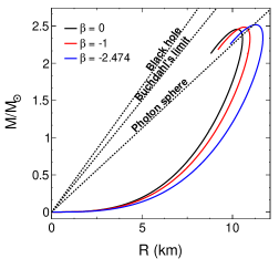
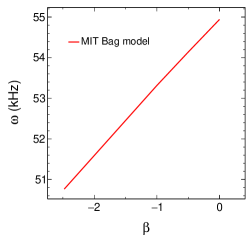
Figure 1: First panel: Variation of mass with radius of strange stars for the MIT Bag model EoS. Second panel: Variation of GWE frequencies within the allowed range of $\beta$ for the MIT Bag model EoS. Here (and also in rest of the cases) the Bag constant $B=$ ($168$ MeV)⁴ is used.

Table 1: Parameters of strange stars for the MIT Bag model EoS with the Bag constant $B=$ ($168$ MeV)⁴.

$\beta$	Radius (R)	Mass (M)	Compactness	GWE	Surface
	(in km)	(in $M_{\odot}$)	(M/R)	frequency (kHz)	redshift (Z)
-2.474	11.28	2.52	0.330	50.75	0.73
-1	10.64	2.49	0.345	53.30	0.82
0	10.26	2.46	0.354	54.94	0.89

The M-R curves for the strange stars with the CFL phase EoS are shown in the left panels of Figs. 2 and 3. For the CFL phase state we have two free parameters, the quark mass $m_{s}$ and the pairing energy gap $\Delta$. With $\Delta=350$ MeV, the M-R curves are showing for different $\beta$ values and for two considered mass cases as $m_{s}=0$ and $m_{s}=100$ MeV in the first panel of Fig. 2. For the first case i.e., $m_{s}=0$ case the $\beta$ value corresponding to the lower limit on compactness is found to be $-0.873$. Thus stellar structures corresponding to $\beta\geq-0.873$ are eligible candidates to have a photon sphere. As in the case of the MIT Bag model, stars corresponding to GR cases are more compact in nature as compared to that in $f(\mathcal{R},T)$ gravity cases. Again, the variation of GWE frequencies with the allowed range of $\beta$ are shown in the second panel of Fig. 2. Monotonically increasing frequencies with increase in $\beta$ values are obtained. On the other hand for $m_{s}=100$ MeV the lower limit of compactness is found to be $-0.813$. As compactness is slightly larger for the massless quark case than the massive quark case, the echo frequencies are also slightly higher for the massless quark case $m_{s}=0$ than that for the massive quark case $m_{s}=100$ MeV. Table. 2 and 3 show distinct values of the different physical parameters of the compact stars under study in these cases.

         

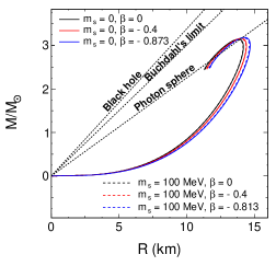
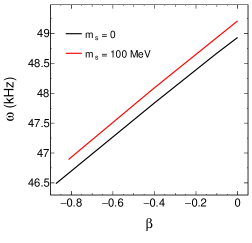
Figure 2: First panel: Variation of mass with radius of strange stars for the CFL phase state with $m_{s}=0$ and $m_{s}=100$ MeV, and with different $\beta$ values. Second panel: Variation of GWE frequencies within allowed range of $\beta$ for the CFL state. Here $\Delta=350$ MeV is used.

Table 2: Parameters of strange stars for the CFL phase with $m_{s}=0$ and $\Delta=350$ MeV.

$\beta$	Radius (R)	Mass (M)	Compactness	GWE
	(in km)	(in $M_{\odot}$)	(M/R)	frequency (kHz)
-0.873	14.28	3.19	0.330	46.48
-0.40	14.02	3.16	0.333	47.33
0	13.82	3.14	0.336	48.93

Table 3: Parameters of strange stars for the CFL phase with $m_{s}=100$ and $\Delta=350$ MeV.

$\beta$	Radius (R)	Mass (M)	Compactness	GWE	Surface
	(in km)	(in $M_{\odot}$)	(M/R)	frequency (kHz)	redshift (Z)
-0.813	14.22	3.17	0.330	46.89	0.74
-0.40	14.00	3.15	0.333	48.08	0.75
0	13.80	3.13	0.336	49.21	0.78

Now, choosing a value of $\beta$ in its allowed range as $\beta=-0.5$, the significance of pairing energy gap $\Delta$ on mass, radius and hence compactness can be visualized from Fig. 3 and Tables 4, 5. In the first panel of Fig. 3 the M-R curves are shown while varying $\Delta$ for $m_{s}=0$ and $m_{s}=100$ MeV. Now for the considered $\beta$ value the minimum value of $\Delta$ needed to support photon sphere is $330.12$ MeV for the case of $m_{s}=0$ and $333.9$ MeV for the case of $m_{s}=100$ MeV. While approaching to a larger value of $\Delta$ the compactness increases vary slightly. Again echo frequencies decrease exponentially with increase in $\Delta$ values as shown in the right panel of Fig. 3. For the two masses, the echo frequencies are found to be nearly equal for all the $\Delta$ values.

         

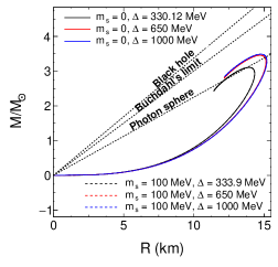
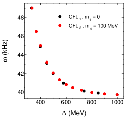
Figure 3: First panel: Variation of mass with radius of strange stars with the MIT Bag model EoS. Second panel: Variation of GWE frequencies with respect to the energy gap $\Delta$. Here the value of $\beta=-0.5$ is used.

Table 4: Parameters of strange stars for the CFL phase with $m_{s}=0$ and $\beta=-0.50$.

$\Delta$	Radius (R)	Mass (M)	Compactness	GWE
(in MeV)	(in km)	(in $M_{\odot}$)	(M/R)	frequency (kHz)
330.12	13.93	3.11	0.330	49.03
650	14.70	3.46	0.348	40.47
1000	14.76	3.49	0.349	39.71

Table 5: Parameters of strange stars for the CFL phase with $m_{s}=100$ and $\beta=-0.50$.

$\Delta$	Radius (R)	Mass (M)	Compactness	GWE
(in MeV)	(in km)	(in $M_{\odot}$)	(M/R)	frequency (kHz)
333.9	13.93	3.11	0.330	49.03
650	14.70	3.46	0.348	40.47
1000	14.76	3.49	0.349	39.71

V Physical properties of stellar structures

Besides the study of M-R curves, which indeed is an important point to study the stellar structures, there are some other physical parameters that need to be addressed. So in this section some physical parameters of strange star configurations viz., metric potential, surface redshift, adiabatic index are discussed briefly.

As mentioned in earlier sections, the present study focuses on two EoSs to describe strange quark matter. The first one is the MIT Bag model EoS and the other is the interacting quark matter EoS. For these two EoSs with the Bag constant $B=(168\mbox{MeV})^{4}$ the variations of compactness of strange stars within a range of $\beta$ values, i.e.  within a range of values of the model parameter of the $f(\mathcal{R},T)$ gravity are shown in Fig. 4. For all the considered cases of EoSs almost linear variations are observed. With a large $\beta$ value the stellar structure with a large compactness is obtained. Also the compactness of stars with the MIT Bag model EoS along the entire range of $\beta$ values is larger as compared to that of CFL phases. The CFL phase with $m_{s}=0$ is more compact than that of the massive case i.e., $m_{s}=100$ MeV. For these CFL phases the pairing energy gap is considered to be $\Delta=350$ MeV.

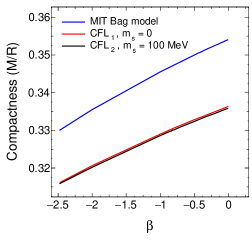
Figure 4: Variation of compactness of stellar structure with the $F(\mathcal{R},T)$ gravity model parameter $\beta$ for the MIT Bag model and the CFL phase of quark states. The Bag constant $B=(168\mbox{MeV})^{4}$ and the energy gap $\Delta=350$ MeV are used in the respective plots.

The pairing energy plays an important role in the compactness of stellar structures. So, the variation of compactness with $\Delta$ is shown in Fig. 5. We have noticed that for small pairing gaps $\Delta$ (lying between 0 to $\sim 600$ MeV) the variation of compactness is rapid. After that range the compactness saturates slowly. Also the stellar configurations with $\Delta\geq 330$ MeV are found to be compact enough to have a photon sphere around their stellar surface. For the maximum $\Delta$ value, $1000$ MeV, compact stars with maximum compactness of about $0.349$. In Fig. 5, for both the mass values, the $f(\mathcal{R},T)$ gravity model parameter $\beta$ is taken as $-0.50$.

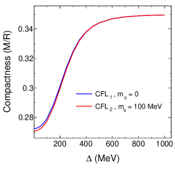
Figure 5: Variation of compactness of stellar structure with pairing gap parameter $\Delta$ for the CFL phase of quark states. Here the value of $\beta$ is taken as $-0.50$.

The behaviour of the metric function $e^{\lambda}$ in the stellar object is shown in Fig. 6. From equation (8) it is seen that $e^{\chi}$, $e^{\lambda}\neq 0$, this indicates that the model is acceptable and physically realistic mustafa . In the left panel of Fig. 6 the variation of the metric function is shown for the case of the MIT Bag model EoS and for the CFL phase EoS with $m_{s}=100$ MeV it is shown in the right panel. It is clear from these two plots that the metric function increases monotonically inside the stellar object.

         

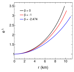
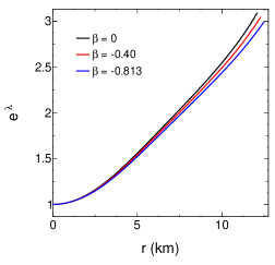
Figure 6: Evolution of metric functions with radial distance $r$ for a) MIT Bag model and b) CFL phase states.

Another important parameter to comment on the stability of relativistic objects is the surface redshift. It is related to the compactness of the stellar structure and hence it plays an important role in describing stability of resulting structures. It describes the relation between the interior geometry of the star and its EoS. Here in this study we have considered stellar structures which are isotropic, static, spherically symmetric in nature and their matter can be described with perfect fluid matter. The compactification factor for such a star can be given as

$$u(r)=\dfrac{m(r)}{r}.$$ (30)

In terms of this compactification factor the surface redshift of a star can be obtained as

$$Z=\dfrac{1}{\sqrt{(1-2u)}}-1.$$ (31)

It is reported that for an isotropic stable stellar configuration the surface redshift $Z\leq 2$ buchdahl ; baraco . For the case of the MIT Bag model the variation of redshift with radial distance $r$ is shown in the first panel of Fig. 7. With the radial distance it increases and attains its maximum value at the surface of the star. The values of these surface redshifts are listed in Table 1 for the MIT Bag model EoS. It is noted that surface redshift is maximum for $\beta=0$ case i.e., the for the GR case and minimum for $\beta=-2.474$. Also for all the considered $\beta$ maximum redshift values are less than unity and hence eventually imply the stability of these structures.

         

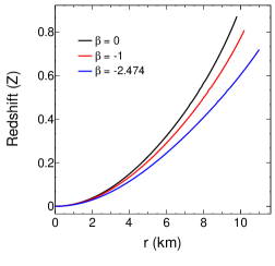
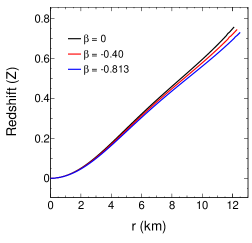
Figure 7: Variation of surface redshift of the stellar structure with radial distance $r$ (in km) for a) MIT Bag model and b) CFL phase EoS with different $\beta$ values.

For the CFL case with $m_{s}=100$ MeV, the variation of redshift is shown in the second panel of Fig. 7 and the respective values are listed in Table 3 for the allowed range of $\beta$. Similar to the case of the MIT Bag model, for this EoS also redshift increases with increase in radial distance and redshift is maximum for $\beta=0$. All these redshift values are such that they respect the stability criteria of isotropic fluid spheres.

To check a region of stability of relativistic isotropic fluid spheres relativistic adiabatic index $\Gamma$ plays an important role. For the spherically symmetric spacetime with a perfect fluid the pioneering work on instability regimes using this adiabatic index was done by Chandrasekhar Chandrasekhar1964a . This adiabatic index directly follows from the radial perturbations of a spherical star mtw . For such stars the stability is only ensured when the fundamental mode of radial oscillations is a real quantity i.e., $\omega^{2}>0$ mtw . For stability of an isotropic sphere $\Gamma>4/3$ and violation with lower $\Gamma$ values indicates instability in the stellar configuration. This adiabatic index can be defined as

$$\Gamma=\dfrac{p+\rho}{p}\,\dfrac{dp}{d\rho}.$$ (32)

For a fully Newtonian case, the stability is maintained for $\Gamma>4/3$ mtw ; hh . For the case of relativistic stars it is required that $\Gamma>\Gamma_{critical}$ where mous ,

$$\Gamma_{critical}=\dfrac{4}{3}+\alpha\dfrac{M}{R}$$ (33)

with $\alpha$ being a small positive quantity and $M/R$ is the compactness of the star.

Now for the considered cases of the present study, the variation of adiabatic index $\Gamma$ with the radial distance $r$ is shown in Fig. 8. The left panel and right panel of this figure corresponds to the MIT Bag model and CFL phase of strange quark matter. The adiabatic index is minimum near the center of the star. These minimum values for all these cases are greater than $4/3$. So it can be inferred that the stellar structures obtained in this study are stable in nature.

         

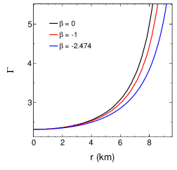
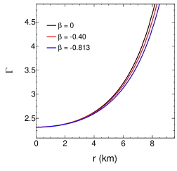
Figure 8: Variation of the adiabatic index with radial distance for a) MIT Bag model and b) CFL phase of quark states.

Furthermore, as discussed in the previous section, for the case of ultracompact rotating stars, ergoregion instability and non-linear instabilities may occur. In the present study such instabilities can be avoided due to the prior consideration of static configuration. However, in a realistic scenario, the presence of these compact objects are associated with such instabilities.

VI Summary and Conclusions

In this work we have studied the compact stars in the context of $f(\mathcal{R},T)$ theory. The $f(\mathcal{R},T)$ gravity model used in this study is one of the widely used models viz., $f(\mathcal{R},T)=\mathcal{R}+2\beta T$. Using the modified TOV equations for this $f(\mathcal{R},T)$ gravity model together with two EoSs, one is the MIT Bag model and other is the interacting quark matter EoS, we have obtained different stellar solutions. Moreover, for the first time in this work GWE frequencies are calculated using realistic CFL induced EoS in the scope of $f(\mathcal{R},T)$ gravity. The stability of the obtained solutions are also analysed. For the considered cases of EoSs, we have constrained the model parameter of the $f(\mathcal{R},T)$ gravity from the perspective of compactness. We have found that to feature a photon sphere above the stellar surface the minimum value of $\beta$ should be $-2.474$ for the stellar structures depicted by the stiffer MIT Bag model. The massless CFL case demands a range of $\beta$ as $-0.873<\beta<0$. Whereas for $m_{s}=100$ MeV, the lower limit of $\beta$ changes to $\beta>-0.813$. As discussed earlier for the stable equilibrium configurations only negative $\beta$ values are allowed. So the constraint $\beta$ values are obtained while respecting this stability condition. An important point obtained from this study is that it is possible to get compact stars with realistic interacting quark matter EoS or the CFL phase state which are able to echo GWs. Moreover, beside the stability condition discussed in this work, another important condition for stability against radial perturbations of any physical system is that the eigenfrequency of the lowest normal mode must be real hh . For the case of compact star like strange star in $f(\mathcal{R},T)=\mathcal{R}+\beta T$ and using MIT Bag model EoS such stability was discussed earlier in the Ref. pretel .

These frequencies of GWEs can play an important role in determining the properties of a host of compact stars. The experimental detection of such frequency will definitely elucidate the internal composition and physical properties of compact stars. The echo frequencies calculated in this study are from the theoretical basis. The prediction of echo frequencies will be of great use once experimental detection of echo frequencies are possible. At present GW detectors like, Advanced LIGO ligo , Advanced Virgo virgo and KAGRA kagra are projected at GWs with frequencies of $\sim 20$ Hz - $4$ kHz and with amplitudes of $\sim 2\times 10^{-22}$ - $4\times 10^{-24}$ strain/$\sqrt{\mbox{Hz}}$ martynov ; abbot . A sensitivity of $\geq 2\times 10^{-23}$ strain/$\sqrt{\mbox{Hz}}$ at $3$ kHz are currently running at LIGO currentligo and Virgo currentvirgo observatories. Again the proposed third generation detectors like Cosmic Explorer (CE) abbott and Einstein Telescope (ET) punturo with optimal arm length of $\approx 20$ km would have the sensitivity to detect neutron star oscillations punturo . The CE may have sensitivity below $10^{-25}$ strain/$\sqrt{\mbox{Hz}}$ at above a few kHz frequencies. Whereas, ET will be able to reach the sensitivity of $>3\times 10^{-25}$ strain/$\sqrt{\mbox{Hz}}$ at $100$ Hz and of $\sim 6\times 10^{-24}$ strain/$\sqrt{\mbox{Hz}}$ at $\sim 10$ kHz. Using some enhancement techniques of the sensitivity of these present and near future detectors it would be possible to detect such frequencies of GWs martynov ; danilishin . So we are optimistic for the detection of such frequencies and thereafter to resolve all the mysteries of the interior of compact stars. In this regard such theoretical prediction will be very handy as it will lead one to know the accurate EoS and hence the properties of the star.

Finally, it needs to be mentioned that in this present work, the echoes from compact stellar objects are studied through the echo timescale between successive excitations of the photon sphere and the stellar surface. It is a very initial technique to analyse echoes of GWs. In this regard the time evolutions techniques are required in order to evolve perturbations on such configurations. However keeping in view of the context of the present work, we have kept it as a possible future direction of the study.

References

- (1) B. P. Abbott et al., Observation of Gravitational Waves from a Binary Black Hole Merger, Phys. Rev. Lett. 116, 061102 (2016).
- (2) B. P. Abbott et al., LIGO: The Laser Interferometer Gravitational-Wave Observatory, Rep. Prog. Phys. 72, 076901 (2009).
- (3) A. G. Riess et. al., Observational Evidence from Supernovae for an Accelerating Universe and a Cosmological Constant, ApJ 116, 1009 (1998).
- (4) S. Perlmutter et. al., Measurements of and from 42 High‐Redshift Supernovae, ApJ 517, 565 (1999).
- (5) G. Bertone and D. Hooper, History of Dark Matter, Rev. Mod. Phys. 90, 045002 (2018).
- (6) K. S. Stelle, Renormalization of Higher-Derivative Quantum Gravity, Phys. Rev. D 16, 953 (1977).
- (7) H. Grigorian, D. N. Voskresensky, and D. Blaschke, Influence of the Stiffness of the Equation of State and In-Medium Effects on the Cooling of Compact Stars, Eur. Phys. J. A 52, 67 (2016).
- (8) A. Li, F. Huang, and R.-X. Xu, Too Massive Neutron Stars: The Role of Dark Matter?, Astropart. Phys. 37, 70 (2012).
- (9) T. P. Sotiriou and V. Faraoni, F(R) Theories of Gravity, Rev. Mod. Phys. 82, 451 (2010).
- (10) A. De Felice and S. Tsujikawa, F(R) Theories, Living Rev. Relativ. 13, 3 (2010).
- (11) T. Harko, F. S. N. Lobo, S. Nojiri, and S. D. Odintsov, Gravity, Phys. Rev. D 84, 024020 (2011).
- (12) T. Harko and F. S. N. Lobo, Gravity, Eur. Phys. J. C 70, 373 (2010).
- (13) S. Carloni, J. L. Rosa, and J. P. S. Lemos, Cosmology of Gravity, Phys. Rev. D 99, 104001 (2019).
- (14) Y.-F. Cai, S. Capozziello, M. De Laurentis, and E. N. Saridakis, f(T) Teleparallel Gravity and Cosmology, Rep. Prog. Phys. 79, 106901 (2016).
- (15) P. Rastall, Generalization of the Einstein Theory, Phys. Rev. D 6, 3357 (1972).
- (16) N. A. Bahcall, J. P. Ostriker, S. Perlmutter, and P. J. Steinhardt, The Cosmic Triangle: Revealing the State of the Universe, Science 284, 1481 (1999).
- (17) J. Hwang and H. Noh, f(R) Gravity Theory and CMBR Constraints, Phys. Lett. B 506, 13 (2001).
- (18) M. Demianski, E. Piedipalumbo, C. Rubano, and C. Tortora, Accelerating Universe in Scalar Tensor Models-Comparison of Theoretical Predictions with Observations, A&A 454, 55 (2006).
- (19) V. Singh and C. P. Singh, Modified f(R,T) Gravity Theory and Scalar Field Cosmology, Astrophys. Space Sci. 356, 153 (2015).
- (20) K. V. Staykov, D. D. Doneva, S. S. Yazadjiev, and K. D. Kokkotas, Slowly Rotating Neutron and Strange Stars in R 2 Gravity, J. Cosmol. Astropart. Phys. 10, 006 (2014).
- (21) A. M. Oliveira, H. E. S. Velten, J. C. Fabris, and L. Casarini, Neutron Stars in Rastall Gravity, Phys. Rev. D 92, 044020 (2015).
- (22) G. Panotopoulos, D. Vernieri, and I. Lopes, Quark Stars with Isotropic Matter in Hořava gravity and Einstein-æther theory, Eur. Phys. J. C 80, 537 (2020).
- (23) G. Herzog and H. Sanchis-Alepuz, Neutron Stars in Palatini and Theories, Eur. Phys. J. C 81, 888 (2021).
- (24) G. G. L. Nashed and S. Capozziello, Anisotropic Compact Stars in f(R) Gravity, Eur. Phys. J. C 81, 481 (2021).
- (25) J. M. Z. Pretel and S. B. Duarte, Anisotropic Quark Stars in Gravity, Class. Quantum Grav. 39, 155003 (2022).
- (26) F. A. Silveira, R. Maier, and S. E. Perez Bergliaffa, A Model of Compact and Ultracompact Objects in -Palatini Theory, Eur. Phys. J. C 81, 7 (2021).
- (27) M. Zubair, G. Abbas, and I. Noureen, Possible Formation of Compact Stars in Gravity, Astrophys. Space Sci. 361, 8 (2016).
- (28) A. Das, F. Rahaman, B. K. Guha, and S. Ray, Compact Stars in Gravity, Eur. Phys. J. C 76, 654 (2016).
- (29) P. H. R. S. Moraes, J. D. V. Arbañil, and M. Malheiro, Stellar Equilibrium Configurations of Compact Stars in f(R ,T) Theory of Gravity, J. Cosmol. Astropart. Phys. 06, 005 (2016).
- (30) D. Deb, F. Rahaman, S. Ray, and B. K. Guha, Strange Stars in Gravity, J. Cosmol. Astropart. Phys. 03, 044 (2018).
- (31) Z. Yousaf, M. Z.-H. Bhatti, and M. Ilyas, Existence of Compact Structures in f(R, T) Gravity, Eur. Phys. J. C 78, 307 (2018).
- (32) R. Lobato, O. Lourenço, P. H. R. S. Moraes, C. H. Lenzi, M. de Avellar, W. de Paula, M. Dutra, and M. Malheiro, Neutron Stars in f(R,T) Gravity Using Realistic Equations of State in the Light of Massive Pulsars and GW170817, J. Cosmol. Astropart. Phys. 12, 039 (2020).
- (33) G. Mustafa, M. Zubair, S. Waheed, and X. Tiecheng, Realistic Stellar Anisotropic Model Satisfying Karmarker Condition in f(R,T) Gravity, Eur. Phys. J. C 80, 26 (2020).
- (34) J. M. Z. Pretel, S. E. Jorás, R. R. R. Reis, and J. D. V. Arbañil, Radial Oscillations and Stability of Compact Stars in Gravity, J. Cosmol. Astropart. Phys. 04, 064 (2021).
- (35) J. M. Z. Pretel, T. Tangphati, A. Banerjee, and A. Pradhan, Charged Quark Stars in Gravity, Chinese Phys. C 46, 115103 (2022).
- (36) P. Rej and P. Bhar, Charged Strange Star in Gravity with Linear Equation of State, Astrophys. Space Sci. 366, 35 (2021).
- (37) E. Witten, Cosmic Separation of Phases, Phys. Rev. D 30, 272 (1984).
- (38) M. Alford, M. Braby, M. Paris, and S. Reddy, Hybrid Stars That Masquerade as Neutron Stars, ApJ 629, 969 (2005).
- (39) G. Lugones and J. E. Horvath, Color-Flavor Locked Strange Matter, Phys. Rev. D 66, 074017 (2002).
- (40) M. Alford, K. Rajagopal, S. Reddy, and F. Wilczek, Minimal Color-Flavor-Locked–Nuclear Interface, Phys. Rev. D 64, 074017 (2001).
- (41) V. Cardoso, E. Franzin, and P. Pani, Is the Gravitational-Wave Ringdown a Probe of the Event Horizon?, Phys. Rev. Lett. 116, 171101 (2016).
- (42) V. Cardoso, S. Hopper, C. F. B. Macedo, C. Palenzuela, and P. Pani, Echoes of ECOs: Gravitational-Wave Signatures of Exotic Compact Objects and of Quantum Corrections at the Horizon Scale, Phys. Rev. D 94, 084031 (2016).
- (43) P. Pani and V. Ferrari, On Gravitational-Wave Echoes from Neutron-Star Binary Coalescences, Class. Quantum Grav. 35, 15LT01 (2018).
- (44) V. Cardoso and P. Pani, Testing the Nature of Dark Compact Objects: A Status Report, Living Rev. Relativ. 22, 4 (2019).
- (45) C. Vlachos, E. Papantonopoulos, and K. Destounis, Echoes of Compact Objects in Scalar-Tensor Theories of Gravity, Phys. Rev. D 103, 044042 (2021).
- (46) N. Chatzifotis, C. Vlachos, K. Destounis, and E. Papantonopoulos, Stability of Black Holes with Non-Minimally Coupled Scalar Hair to the Einstein Tensor, Gen. Relativ. Gravit. 54, 49 (2022).
- (47) M. Mannarelli and F. Tonelli, Gravitational Wave Echoes from Strange Stars, Phys. Rev. D 97, 123010 (2018).
- (48) A. Urbano and H. Veerm ae, On Gravitational Echoes from Ultracompact Exotic Stars, J. Cosmol. Astropart. Phys. 04, 011 (2019).
- (49) J. Bora and U. D. Goswami, Radial Oscillations and Gravitational Wave Echoes of Strange Stars for Various Equations of State, Monthly Notices of the Royal Astronomical Society 502, 1557 (2021).
- (50) C. Zhang, Gravitational Wave Echoes from Interacting Quark Stars, Phys. Rev. D 104, 083032 (2021).
- (51) J. Bora and U. D. Goswami, Radial oscillations and gravitational wave echoes of strange stars with nonvanishing lambda, Astropart. Phys. 143, 102744 (2022).
- (52) J. Bora, D. J. Gogoi and U. D. Goswami, Strange stars in gravity Palatini formalism and gravitational wave echoes from them, J. Cosmol. Astropart. Phys. 09, 057 (2022).
- (53) J. Wu, G. Li, T. Harko and S.-D. Liang, Palatini formulation of f(R,T) gravity theory, and its cosmological implications, Europ. Phys. J. C 78 430 (2018) [arxiv:1805.07419].
- (54) J. Barrientos O. and G. F. Rubilar, Surface curvature singularities of polytropic spheres in Palatini gravity, Phys. Rev. D 93 024021 (2016).
- (55) M. Z. Bhatti, Z. Yousaf and Zarnoor, Stability analysis of neutron stars in Palatini f(R,T) gravity, Gen. Relat. Grav. 51 144 (2019).
- (56) G. A. Carvalho, R. V. Lobato, P. H. R. S. Moraes, J. D. V. Arbañil, E. Otoniel, R. M. Marinho, and M. Malheiro, Stellar Equilibrium Configurations of White Dwarfs in the f(R,T) Gravity, Eur. Phys. J. C 77, 871 (2017).
- (57) S. Bhattacharjee and P. K. Sahoo, Constraining Gravity from the Dark Energy Density Parameter , Gravit. Cosmol. 26, 281 (2020).
- (58) H. Velten and T. R. P. Caramês, Cosmological Inviability of f(R,T) Gravity, Phys. Rev. D 95, 123536 (2017).
- (59) H. Maulana and A. Sulaksono, Impact of Energy-Momentum Nonconservation on Radial Pulsations of Strange Stars, Phys. Rev. D 100, 124014 (2019).
- (60) C. V. Flores and G. Lugones, Constraining Color Flavor Locked Strange Stars in the Gravitational Wave Era, Phys. Rev. C 95, 025808 (2017).
- (61) E. Farhi and R. L. Jaffe, Strange Matter, Phys. Rev. D 30, 2379 (1984).
- (62) J. Beringer et al., Review of Particle Physics, Phys. Rev. D 86, 010001 (2012).
- (63) J. L. Friedman, Ergosphere Instability, Commun. Math. Phys. 63, 243 (1978).
- (64) N. Comins, B. F. Schutz, and S. Chandrasekhar, On the Ergoregion Instability, Proceedings of the Royal Society of London. A. Mathematical and Physical Sciences 364, 211 (1978).
- (65) V. Cardoso, P. Pani, M. Cadoni, and M. Cavaglia, Ergoregion Instability of Ultra-Compact Astrophysical Objects, Phys. Rev. D 77, 124044 (2008).
- (66) C. B. M. H. Chirenti and L. Rezzolla, On the Ergoregion Instability in Rotating Gravastars, Phys. Rev. D 78, 084011 (2008).
- (67) J. Keir, Slowly Decaying Waves on Spherically Symmetric Spacetimes and an Instability of Ultracompact Neutron Stars, arXiv:1404.7036 [gr-qc].
- (68) V. Cardoso, L. C. B. Crispino, C. F. B. Macedo, H. Okawa, and P. Pani, Light Rings as Observational Evidence for Event Horizons: Long-Lived Modes, Ergoregions and Nonlinear Instabilities of Ultracompact Objects, Phys. Rev. D 90, 044069 (2014).
- (69) G. Moschidis, A Proof of Friedman’s Ergosphere Instability for Scalar Waves, arXiv:1608.02035 [math.AP].
- (70) P. V. P. Cunha, C. Herdeiro, E. Radu, and N. Sanchis-Gual, The Fate of the Light-Ring Instability, arXiv:2207.13713 [gr-qc].
- (71) V. Boyanov, K. Destounis, R. P. Macedo, V. Cardoso, and J. L. Jaramillo, Pseudospectrum of Horizonless Compact Objects: A Bootstrap Instability Mechanism, arXiv:2209.12950 [gr-qc].
- (72) H. A. Buchdahl, General Relativistic Fluid Spheres, Phys. Rev. 116, 1027 (1959).
- (73) P. Burikham, T. Harko, and M. J. Lake, Mass Bounds for Compact Spherically Symmetric Objects in Generalized Gravity Theories, Phys. Rev. D 94, 064070 (2016).
- (74) D. Barraco and V. H. Hamity, Maximum Mass of a Spherically Symmetric Isotropic Star, Phys. Rev. D 65, 124028 (2002).
- (75) S. Chandrasekhar, The Dynamical Instability of Gaseous Masses Approaching the Schwarzschild Limit in General Relativity, ApJ 140, 417 (1964).
- (76) H. Heintzmann and W. Hillebrandt, Neutron Stars with an Anisotropic Equation of State: Mass, Redshift and Stability, A&A 38, 51 (1975).
- (77) C. W. Misner, K. S. Thorne, and J. A. Wheeler, Gravitation (W. H. Freeman, San Francisco, 1973).
- (78) Ch. C. Moustakidis, The Stability of Relativistic Stars and the Role of the Adiabatic Index, Gen. Relat. Grav. 49, 68 (2017).
- (79) W. Hillebrandt and K. O. Steinmetz, Anisotropic Neutron Star Models: Stability against Radial and Nonradial Pulsations, A&A 53, 283 (1976).
- (80) J. Aasi et al., Advanced LIGO, Class. Quantum Grav. 32, 074001 (2015).
- (81) F. Acernese et al., Advanced Virgo: A Second-Generation Interferometric Gravitational Wave Detector, Class. Quantum Grav. 32, 024001 (2015).
- (82) Y. Aso, Y. Michimura, K. Somiya, M. Ando, O. Miyakawa, T. Sekiguchi, D. Tatsumi, and H. Yamamoto, Interferometer Design of the KAGRA Gravitational Wave Detector, Phys. Rev. D 88, 043007 (2013).
- (83) D. Martynov et al., Exploring the Sensitivity of Gravitational Wave Detectors to Neutron Star Physics, Phys. Rev. D 99, 102004 (2019).
- (84) B. Abbott et al., Prospects for Observing and Localizing Gravitational-Wave Transients with Advanced LIGO, Advanced Virgo and KAGRA, Living Rev. Relativ. 23, 3 (2020).
- (85) B. Caron et al., The Virgo interferometer, Class. Quantum Grav. 14, 1461 (1997).
- (86) B. Abbott et al., GW170817: Observation of Gravitational Waves from a Binary Neutron Star Inspiral, Phys. Rev. Lett. 119, 161101 (2017).
- (87) M. Punturo et al., The Einstein Telescope: A Third-Generation Gravitational Wave Observatory, Class. Quantum Grav. 27, 194002 (2010).
- (88) S. L. Danilishin, F. Y. Khalili , H. Miao, Advanced Quantum Techniques for Future Gravitational-Wave Detectors, Living Rev. Relativ. 22, 2 (2019).