Robust second-order approximation of the compressible Euler equations with an arbitrary equation of state

Abstract

This paper is concerned with the approximation of the compressible Euler equations supplemented with an arbitrary or tabulated equation of state. The proposed approximation technique is robust, formally second-order accurate in space, invariant-domain preserving, and works for every equation of state, tabulated or analytic, provided the pressure is nonnegative. An entropy surrogate functional that grows across shocks is proposed. The numerical method is verified with novel analytical solutions and then validated with several computational benchmarks seen in the literature.

65M60, 65M12, 65M15, 35L45, 35L65

1 Introduction

The objective of this paper is to continue the work started in Clayton et al. [6] where we introduced an explicit and invariant-domain preserving method to approximate the Euler equations equipped with an equation of state that is either tabulated or is given by an expression that is so involved that elementary Riemann problems cannot be solved exactly or efficiently. The method proposed in [6] is invariant-domain preserving in the sense that it guarantees that the density and the internal energy of the approximation are positive. A key ingredient of the method is a local approximation of the equation of state using a covolume ansatz (a.k.a. Noble-Abel equation of state) from which upper bounds on the maximum wave speed are derived for every elementary Riemann problem. The downside is that the method is first-order accurate in space. In the present paper we propose a technique that increases the accuracy in space to second-order and preserves the invariant-domain properties. We also introduce a functional that can be used as an entropy surrogate. The functional in question is shown to be increasing across shocks in the Riemann problem involved in the construction of the local maximum wave speed. We show how to use this functional to limit the internal energy from below. This feature is useful for equations of state that are tabulated or interpolated from experimental data since in this case no natural notion of entropy is available.

It is sometimes possible, though possibly expensive, to solve Riemann problems when the equation of state is analytic. For instance this is done in Colella and Glaz [7, §1], Ivings et al. [23], Quartapelle et al. [32]. This cannot be done with tabulated equations of state because the information on the pressure is incomplete. Several attempts to develop methods working with an arbitrary or tabulated equation of state have been reported in the literature. One way to do so consists of using approximate Riemann solvers like those found in Dukowicz [8], [7, §2], Roe and Pike [34], Pike [31], and Lee et al. [25]. One can also simplify the Riemann problem by using flux splitting techniques as those reported in Toro et al. [39]. We also refer to Saurel et al. [35], Banks [1], Dumbser and Casulli [9], Dumbser et al. [10] where approximation techniques are developed using approximate Riemann solvers for various equations of state. Some of these techniques guarantee positivity of the density, but little else is guaranteed in general. The method introduced in Clayton et al. [6] is based on a graph viscosity technique using upper bounds on the maximum wave speed in the Riemann problem. Instead of using the two-shock approximation of the Riemann solution, as done in most methods based on approximate solvers, the method proposed in [6] approximates the pressure in the Riemann fan by the covolume equation of state and subsequently estimates guaranteed upper bounds on the maximum wave speed. This in turn ensures that the internal energy in the proposed algorithm is positive in addition to the density being positive. If it happens that the equation of state is of covolume type, then the method also preserves the minimum principle on the specific entropy. A technique based on similar principles is reported in Wang and Li [40] where the authors use a stiffened gas equation of state to approximate the pressure in the Riemann fan. To the best of our knowledge, the method proposed in the present paper is among the very first ones that are provably invariant-domain preserving for complex or tabulated equations of state and high-order accurate in space.

The paper is organized as follows. In Section 2, we introduce the mathematical model of interest and the corresponding notation. We also briefly discuss the assumptions we make on the equation of state and recall results from [6] that are needed for this work (i.e., we recall the first-order approximation of the Euler equations in §2.3). In Section 3, we construct a provisional update that is higher-order accurate in space. This update is based on a high-order graph viscosity using an entropy commutator and an activation function. Then, in Section 4, we apply a novel convex limiting technique that corrects the invariant-domain violations of the provisional higher-order method. The final result is an approximation technique that is robust, formally second-order accurate in space, provably invariant-domain preserving, and works for every equation of state (tabulated or analytic) that satisfies the mild assumptions stated in §2.2. Finally in Section 5, the method is verified with analytical solutions and published benchmarks and is validated with experiments. A short conclusion is given in §6.

2 Preliminaries

We formulate the problem and introduce notation in this section. We also recall essential results from [6] for completeness.

2.1 The Euler equations

Let $D$ be a bounded polyhedron in ${\mathbb{R}}^{d}$. Given some initial data ${\bm{u}}_{0}({\bm{x}}):=(\rho_{0},{\bm{m}}_{0},E_{0})({\bm{x}})$ and initial time $t_{0}$, we look for ${\bm{u}}({\bm{x}},t):=(\rho,{\bm{m}},E)({\bm{x}},t)$ solving the compressible Euler equations in the weak sense:

(2.1a) $$\partial_{t}\rho+\nabla{\cdot}({\bm{v}}\rho)=0 \text{a.e.\@ $t>t_{0}$, ${\bm{x}}\in D$},$$

(2.1b) $$\partial_{t}{\bm{m}}+\nabla{\cdot}\big{(}{\bm{v}}\otimes{\bm{m}}+p({\bm{u}}){\mathbb{I}}_{d}\big{)}={\bm{0}} \text{a.e.\@ $t>t_{0}$, ${\bm{x}}\in D$},$$

(2.1c) $$\partial_{t}E+\nabla{\cdot}\big{(}{\bm{v}}(E+p({\bm{u}}))\big{)}=0 \text{a.e.\@ $t>t_{0}$, ${\bm{x}}\in D$}.$$

The components of the dependent variable ${\bm{u}}:=(\rho,{\bm{m}},E)^{\mathsf{T}}\in{\mathbb{R}}^{d+2}$ (considered to be a column vector) are the density, $\rho$, the momentum, ${\bm{m}}$, and the total mechanical energy, $E$. We also introduce the velocity ${\bm{v}}({\bm{u}}):=\rho^{-1}{\bm{m}}$ and the specific internal energy, $e({\bm{u}}):=\rho^{-1}E-\frac{1}{2}\|{\bm{v}}({\bm{u}})\|_{\ell^{2}}^{2}$. To simplify the notation later on we introduce the flux ${\mathbbm{f}}({\bm{u}}):=({\bm{m}},{\bm{v}}({\bm{u}})\otimes{\bm{m}}+p({\bm{u}}){\mathbb{I}}_{d},{\bm{v}}({\bm{u}})(E+p))^{\mathsf{T}}\in{\mathbb{R}}^{(d+2)\times d}$, where ${\mathbb{I}}_{d}$ is the $d{\times}d$ identity matrix.

2.2 Equation of state

In (2.1) the function $p({\bm{u}})$ denotes the pressure which we assume to be given by an oracle. This means we assume to have no a priori knowledge of the function $p({\bm{u}})$ itself apart from some mild structural assumptions stated below. We only assume that for a given state ${\bm{u}}$ we are able to retrieve a pressure $p({\bm{u}})$ in a suitable way, for example by evaluating an arbitrary analytic expression, or by deriving a value from tabulated experimental data. More precisely, in the numerical illustrations reported in §5, we consider oracles given by analytic functions for the ideal gas, van der Waals, Jones–Wilkins–Lee and Mie-Gruneisen equations of state. We also use the SESAME database developed at Los Alamos National Laboratory [27] to test the method with experimental tabulated data.

Throughout the paper we assume that the domain of definition of the oracle $p({\bm{u}})$ is the set ${\mathcal{B}}(b)\subset{\mathbb{R}}^{d+2}$ given by

(2.2) $${\mathcal{B}}(b):=\big{\{}{\bm{u}}:=(\rho,{\bm{m}},E)\in\mathbb{R}^{d+2}{\;|\;}0<\rho,\ 0<1-b\rho,\;0<e({\bm{u}})\big{\}}.$$

We henceforth refer to ${\mathcal{B}}(b)$ as the admissible set. One of the objectives of the paper is to guarantee that the approximation is high-order accurate and leaves ${\mathcal{B}}(b)$ invariant. The inequality $\rho<\tfrac{1}{b}$ found in the definition of ${\mathcal{B}}(b)$ is the so called maximum compressibility condition. The constant $b$ can be set to zero if the user has no a priori knowledge about the maximum compressibility of the fluid under consideration. We recall, however, that a large class of analytic equations of state, such as the Noble-Abel, the Mie-Gruneisen (with the Hugoniot locus as the reference curve), and the Noble-Abel-Stiffened-Gas equations of state all involve a maximum compressibility constant. Finally, we assume that the oracle $p({\bm{u}})$ returns a non-negative pressure,

(2.3) $$p:{\mathcal{B}}(b)\to{\mathbb{R}}_{\geq 0}.$$

The assumption can be weakened, but for the sake of simplicity, we refrain from doing so in this paper. We leave this extension for future works.

2.3 First-order time and space approximation

The time and space discretization proposed in Clayton et al. [6] is based on [16]. This method is in some sense a discretization-agnostic generalization of an algorithm introduced by Lax [24, p. 163]. We denote by $t^{n}$ the current time, $n\in{\mathbb{N}}$, and we denote by ${\tau}$ the current time step size; that is $t^{n+1}:=t^{n}+{\tau}$. Without going into the details of the space approximation, we assume that the current approximation of ${\bm{u}}(\cdot,t^{n})$ is a collection of states $\{\textsf{{U}}_{i}^{n}\}_{i\in{\mathcal{V}}}$, where the index set ${\mathcal{V}}$ is used to enumerate all the degrees of freedom of the approximation, and $\textsf{{U}}_{i}^{n}$ is in ${\mathbb{R}}^{d+2}$ for all $i\in{\mathcal{V}}$. The update at $t^{n+1}$ is obtained as follows:

(2.4) $$\frac{m_{i}}{{\tau}}(\textsf{{U}}_{i}^{\textup{L},n+1}-\textsf{{U}}_{i}^{n})+\!\!\sum_{j\in{\mathcal{I}}(i)}{\mathbbm{f}}(\textsf{{U}}_{j}^{n})\,{\bm{c}}_{ij}-\!\!\sum_{j\in{\mathcal{I}}(i){\setminus}\{i\}}d_{ij}^{\textup{L},n}(\textsf{{U}}^{n}_{j}-\textsf{{U}}^{n}_{i})={\bm{0}}.$$

The quantity $m_{i}$ is called the lumped mass and we assume that $m_{i}>0$ for all $i\in{\mathcal{V}}$. The vector ${\bm{c}}_{ij}\in{\mathbb{R}}^{d}$ encodes the space discretization. The index set ${\mathcal{I}}(i)$ is called the local stencil. This set collects only the degrees of freedom in ${\mathcal{V}}$ that interact with $i$ (i.e., $j\not\in{\mathcal{I}}(i)\Rightarrow{\bm{c}}_{ij}={\bm{0}}$). We assume that the ${\mathbb{R}}^{d}$-valued coefficients ${\bm{c}}_{ij}$ are such that $\sum_{j\in{\mathcal{I}}(i)}{\mathbbm{f}}(\textsf{{U}}_{j}^{n}){\bm{c}}_{ij}$ approximates $\nabla{\cdot}({\mathbbm{f}}({\bm{u}}(\cdot,t^{n})))$ at some grid point ${\bm{a}}_{i}$, and the consistency error in space scales optimally with respect to the mesh size for the considered approximation setting. We require that the method be conservative; more precisely, we assume that

(2.5) $${\bm{c}}_{ij}=-{\bm{c}}_{ji}\quad\text{and}\quad\sum_{j\in{\mathcal{I}}(i)}{\bm{c}}_{ij}={\bm{0}}.$$

Concrete expressions for ${\bm{c}}_{ij}$ and $m_{i}$ are given in [19, §4] for continuous and discontinuous finite elements as well as for finite volumes. The computations reported at the end of this paper are done with piecewise linear continuous finite elements. But to stay general, we continue with the abstract discretization-agnostic notation introduced above.

For completeness we now recall how the graph viscosity $d_{ij}^{\textup{L},n}$ is defined in [6]. Given $i\in{\mathcal{V}}$ and $j\in{\mathcal{I}}(i)$, we set ${\bm{n}}_{ij}:={\bm{c}}_{ij}\|{\bm{c}}_{ij}\|_{\ell^{2}}^{-1}$. For $Z\in\{i,j\}$, we set $\textsf{{U}}_{Z}:=(\varrho_{Z},\textsf{{M}}_{Z},{\mathsf{E}}_{Z})^{\mathsf{T}},$ ${\mathsf{p}}_{Z}:=p(\textsf{{U}}_{Z}^{n})$, ${\mathsf{e}}_{Z}:=e(\textsf{{U}}_{Z}^{n})$, $\Gamma_{Z}:=\varrho_{Z}+\frac{{\mathsf{p}}_{Z}(1-b\varrho_{Z})}{{\mathsf{e}}_{Z}}$, and $\mathcal{E}_{Z}:={\mathsf{E}}_{Z}-\frac{\|\textsf{{M}}_{Z}-(\textsf{{M}}_{Z}{\cdot}{\bm{n}}_{ij}){\bm{n}}_{ij}\|_{\ell^{2}}^{2}}{2\varrho_{Z}}$. The non-negativity assumption on the pressure (2.3) and the assumptions on the density ($0<\varrho_{Z}<\frac{1}{b}$) implies that

(2.6) $$\gamma_{Z}:=\frac{\Gamma_{Z}}{\varrho_{Z}}\geq 1.$$

Then we consider the following Riemann problem:

(2.7) $$\partial_{t}\begin{pmatrix}\rho\\ m\\ \mathcal{E}\\ \Gamma\end{pmatrix}+\partial_{x}\begin{pmatrix}m\\ \tfrac{1}{\rho}m^{2}+\mathcal{p}_{\text{cov}}\\ \tfrac{m}{\rho}(\mathcal{E}+\mathcal{p}_{\text{cov}})\\ \tfrac{m}{\rho}\Gamma\end{pmatrix}=0,\quad\text{with}\quad\mathcal{p}_{\text{cov}}(\rho,m,{\mathcal{E}},\Gamma):=\frac{\frac{\Gamma}{\rho}-1}{1-b\rho}\left(\mathcal{E}-\tfrac{m^{2}}{2\rho}\right),$$

with left data $(\rho_{i},{\bm{m}}_{i}{\cdot}{\bm{n}}_{ij},\mathcal{E}_{i},\Gamma_{i})^{\mathsf{T}}$ and right data $(\rho_{j},{\bm{m}}_{j}{\cdot}{\bm{n}}_{ij},\mathcal{E}_{j},\Gamma_{j})^{\mathsf{T}}$. This problem is well-posed because $\gamma_{Z}\geq 1$. Its complete solution is given in Clayton et al. [6, §4]. We denote by $\lambda({\bm{n}}_{ij},\textsf{{U}}_{i},\textsf{{U}}_{j})$ the maximum wave speed in this problem. Let ${\mathcal{A}}$ be a nontrivial convex subset of ${\mathcal{B}}(b)$. We say that ${\mathcal{A}}$ is an invariant set for (2.7) if for every pair of Riemann data in ${\mathcal{A}}$ the solution of (2.7) takes values in ${\mathcal{A}}$. We then have:

Theorem 2.1 ([6, Thm. 4.6]).

Let $i\in{\mathcal{V}}$. Let ${\mathcal{A}}\subset{\mathcal{B}}(b)$ be a convex invariant set for (2.7). Assume that $\textsf{{U}}_{j}^{n}\in{\mathcal{A}}$ for all $j\in{\mathcal{I}}(i)$. For all $j\in{\mathcal{I}}(i)$, let ${\widehat{\lambda}}({\bm{n}}_{ij},\textsf{{U}}_{i}^{n},\textsf{{U}}_{j}^{n})$ be any positive number larger than or equal to $\lambda({\bm{n}}_{ij},\textsf{{U}}_{i}^{n},\textsf{{U}}_{j}^{n})$. Let

(2.8) $$d_{ij}^{\textup{L},n}:=\max({\widehat{\lambda}}({\bm{n}}_{ij},\textsf{{U}}_{i}^{n},\textsf{{U}}_{j}^{n})\|{\bm{c}}_{ij}\|_{\ell^{2}},{\widehat{\lambda}}({\bm{n}}_{ji},\textsf{{U}}_{j}^{n},\textsf{{U}}_{i}^{n})\|{\bm{c}}_{ji}\|_{\ell^{2}}).$$

Assume that ${\tau}$ is small enough so that ${\tau}\sum_{j\in{\mathcal{I}}(i){\setminus}\{i\}}\frac{2d_{ij}^{\textup{L},n}}{m_{i}}\leq 1$. Let $\textsf{{U}}_{i}^{\textup{L},n+1}$ be the update defined in (2.4). Then $\textsf{{U}}^{\textup{L},n+1}_{i}\in{\mathcal{A}}\subset{\mathcal{B}}(b)$. $\square$

Remark 2.2 (Invariant domains).

Theorem 2.1 asserts that every convex invariant set in ${\mathcal{B}}(b)$ is invariant by the update procedure (2.4) with the artificial viscosity $d_{ij}^{\textup{L},n}$ defined in (2.8). This means that if $\textsf{{U}}^{n}_{i}\in{\mathcal{A}}$ for all $i\in{\mathcal{V}}$, then $\textsf{{U}}^{\textup{L},n+1}_{i}\in{\mathcal{A}}$ for all $i\in{\mathcal{V}}$. We say that the method is invariant-domain preserving for ${\mathcal{A}}$. Notice in particular that the method is invariant-domain preserving for the admissible set ${\mathcal{B}}(b)$. The admissible set ${\mathcal{B}}(b)$ may not be the smallest invariant domain. For instance, if the oracle admits a mathematical entropy $s$, then the approximation defined above is also invariant-domain preserving for the set ${\mathcal{A}}({\bm{u}}_{0}):=\{{\bm{v}}\in{\mathcal{B}}(b){\;|\;}s({\bm{v}})\geq\operatorname*{ess\,inf}_{{\bm{x}}\in D}s({\bm{u}}_{0}({\bm{x}}))\}$; see e.g., [16, Cor. 4.2]. By slight abuse of terminology and provided the context is unambiguous we will simply call a method invariant-domain preserving without quantifying the precise convex set. $\square$

A source code to compute ${\widehat{\lambda}}({\bm{n}}_{ij},\textsf{{U}}_{i}^{n},\textsf{{U}}_{j}^{n})$ is available online [5]. A notable drawback of the graph viscosity (2.8) is that it reduces the space accuracy of the method to first order. The remainder of the paper is concerned with constructing a higher-order approximation and a respective novel convex limiting technique that is invariant-domain preserving.

Remark 2.3 (Pressure approximation).

Notice that the oracle is only invoked to compute the left and right values of the pressure in (2.7). The pressure in the Riemann fan is approximated by two covolume equations of state. There is one covolume equation of state for each side of the contact discontinuity since $\gamma=\gamma_{L}$ on the left of the contact wave and $\gamma=\gamma_{R}$ on the right. $\square$

3 Provisional higher-order method

In this section, we introduce a provisional higher-order method that extends the update (2.4) to second order when using linear finite elements for the discretization. A convex limiting technique for this provisional update is introduced in §4. The provisional method is based on the work reported in [18, 28].

3.1 The method

Higher-order accuracy in space requires using the consistent mass matrix instead of the lumped mass matrix for the discretization of the time derivative. By reducing dispersive errors, the consistent mass matrix is known to yield superconvergence at the grid points; see e.g., Christon et al. [4], [14], [28, Sec. 3.4], Thompson [38]. Let ${\mathbb{M}}$ be the mass matrix with entries $\{m_{ij}\}_{i,j\in{\mathcal{V}}}$, then ${\mathbb{M}}^{-1}$ can be approximated by ${\mathbb{I}}+{\mathbb{B}}$ where $b_{ij}=\delta_{ij}-\frac{m_{ij}}{m_{j}}$, $\delta_{ij}$ is the Kronecker symbol, and $m_{i}:=\sum_{j\in{\mathcal{I}}(i)}m_{ij}$. This approximation has been shown in [4, 14] to be superconvergent for piecewise-linear continuous finite elements. Let ${\mathsf{R}}\in{\mathbb{R}}^{I}$ with $I:=\text{card}({\mathcal{V}})$, then using this approximation we have $({\mathbb{M}}^{-1}{\mathsf{R}})_{i}\approx{\mathsf{R}}_{i}+\sum_{j\in{\mathcal{I}}(i)}\left(b_{ij}{\mathsf{R}}_{j}-b_{ji}{\mathsf{R}}_{i}\right)$. Notice that $\sum_{j\in{\mathcal{I}}(i)}b_{ji}{\mathsf{R}}_{i}=0$, because $\sum_{j\in{\mathcal{I}}(i)}b_{ji}=0$. The skew-symmetry of the summand in $\sum_{j\in{\mathcal{I}}(i)}\left(b_{ij}{\mathsf{R}}_{j}-b_{ji}{\mathsf{R}}_{i}\right)$ is used in §4 for limiting purposes.

Let $\textsf{{U}}^{\text{H},n+1}$ denote the high-order update (here the superindex ${}^{\textup{H}}$ reminds us that the update is higher order accurate). Then, for every $i\in{\mathcal{V}}$, the provisional high-order update is given by:

(3.1a) $$\frac{m_{i}}{\tau}\left(\textsf{{U}}_{i}^{\text{H},n+1}-\textsf{{U}}_{i}^{n}\right)={\bm{R}}_{i}^{n}+\sum_{j\in{\mathcal{I}}(i)}\left(b_{ij}{\bm{R}}_{j}^{n}-b_{ji}{\bm{R}}_{i}^{n}\right),$$

(3.1b) $$\text{with}\qquad\qquad{\bm{R}}_{i}^{n}:=\sum_{j\in{\mathcal{I}}(i)}\left(-{\mathbbm{f}}(\textsf{{U}}_{j}^{n}){\cdot}{\bm{c}}_{ij}+d_{ij}^{\textup{H},n}(\textsf{{U}}_{j}^{n}-\textsf{{U}}_{i}^{n})\right).$$

The high-order graph viscosity coefficient $d_{ij}^{\textup{H},n}$, defined in Section 3.2, shares the same properties as its low-order counterpart which are necessary for conservation:

(3.2) $$d_{ij}^{\textup{H},n}=d_{ji}^{\textup{H},n},\quad 0\leq d_{ij}^{\textup{H},n}\leq d_{ij}^{\textup{L},n},\quad\text{for every }j\in{\mathcal{I}}(i),\;i\in{\mathcal{V}}.$$

3.2 Entropy commutator

Using the entropy-viscosity methodology introduced in Guermond et al. [17], we now discuss the construction of the high-order graph viscosity coefficient $d_{ij}^{\textup{H},n}$ that is used in the high-order update (3.1b). A complicating factor in this construction is that the pressure is given by an oracle. We thus do not have a priori knowledge on the equation of state and entropies of the system.

Recall that $(\eta({\bm{u}}),{\bm{F}}({\bm{u}}))$ is an entropy pair for the Euler equations if

(3.3) $$\nabla{\cdot}{\bm{F}}({\bm{u}})=(\nabla_{\bm{u}}\eta({\bm{u}}))^{\mathsf{T}}\nabla{\cdot}{\mathbbm{f}}({\bm{u}}),\qquad\forall{\bm{u}}\in{\mathcal{B}}(b),$$

where ${\mathbbm{f}}({\bm{u}})$ is the flux of the system (2.1). Since one may not have access to entropies for tabulated equations of state, we are going to use at every $i\in{\mathcal{V}}$ and every time $t^{n}$ one entropy pair associated with the following flux

(3.4) $${\mathbbm{f}}^{i,n}({\bm{u}}):=\begin{pmatrix}{\bm{m}}\\ {\bm{v}}\otimes{\bm{m}}+\mathcal{p}_{\text{cov}}^{i,n}({\bm{u}}){\mathbb{I}}_{d}\\ {\bm{v}}(E+\mathcal{p}_{\text{cov}}^{i,n}({\bm{u}}))\end{pmatrix},\qquad\mathcal{p}_{\text{cov}}^{i,n}({\bm{u}}):=(\gamma_{i}^{\min,n}-1)\frac{\rho e({\bm{u}})}{1-b\rho}.$$

Here, $\gamma_{i}^{\min,n}:=\min_{j\in{\mathcal{I}}(i)}\gamma_{j}^{n}$ with $\gamma_{j}^{n}:=1+\frac{{\mathsf{p}}_{j}^{n}(1-b\varrho_{j}^{n})}{\varrho_{j}^{n}{\mathsf{e}}_{j}^{n}}$ (see (2.6)). We use the following shifted Harten entropy pair in the numerical tests reported in §5:

(3.5) $$\eta^{i,n}({\bm{u}}):=\left(\frac{\rho^{2}e({\bm{u}})}{(1-b\rho)^{1-\gamma_{i}^{\min,n}}}\right)^{\frac{1}{\gamma_{i}^{\min,n}+1}}-\frac{\rho}{\varrho_{i}^{n}}\eta_{\text{ref}}^{i,n},\qquad{\bm{F}}^{i,n}({\bm{u}}):=\frac{{\bm{m}}}{\rho}\eta^{i,n}({\bm{u}}),$$

where $\eta_{\text{ref}}^{i,n}:=\left(\frac{(\varrho_{i}^{n})^{2}e({\bm{u}}_{i}^{n})}{(1-b\varrho_{i}^{n})^{1-\gamma_{i}^{\min,n}}}\right)^{\frac{1}{\gamma_{i}^{\min,n}+1}}$. Then, we estimate “entropy production” by inserting the approximate solution ${\bm{u}}_{h}^{n}$ into a discrete counterpart of (3.3) which we write as follows:

(3.6) $$\int_{D}\left(\nabla{\cdot}{\bm{F}}^{i,n}({\bm{u}})-(\nabla_{\bm{u}}\eta^{i,n}({\bm{u}}))^{\mathsf{T}}\nabla{\cdot}\,{\mathbbm{f}}^{i,n}({\bm{u}})\right)\varphi_{i}\,{\mathrm{d}}x=0,$$

where $\{\varphi_{i}\}_{i\in{\mathcal{V}}}$ are the shape functions of the finite element approximation. Notice that the above identity holds true for every smooth function ${\bm{u}}\in{\mathcal{B}}(b)$ and for every $i\in{\mathcal{V}}$. Substituting ${\bm{u}}_{h}:=\sum_{i\in{\mathcal{V}}}\textsf{{U}}_{i}^{n}\varphi_{i}$ into (3.6), we estimate the local entropy residual as follows:

(3.7) $$N_{i}^{n}:=\sum_{j\in{\mathcal{I}}(i)}\Big{(}{\bm{F}}^{i,n}(\textsf{{U}}_{j}^{n})-(\nabla_{{\bm{u}}}\eta^{i,n}(\textsf{{U}}_{i}^{n}))^{\mathsf{T}}{\mathbbm{f}}^{i,n}(\textsf{{U}}_{j}^{n})\Big{)}{\cdot}{\bm{c}}_{ij}.$$

The residual (3.7) can be thought of as a measure of how well the discrete solution ${\bm{u}}_{h}^{n}$ satisfies (3.6) in each local stencil ${\mathcal{I}}(i)$. We then define the normalized entropy residual as follows:

(3.8a) $$R_{i}^{n} :=\frac{\left|N_{i}^{n}\right|}{D_{i}+\epsilon D^{\max}},\qquad D^{\max}=\max_{i\in{\mathcal{V}}}D_{i},\qquad\epsilon=10^{-2},$$

(3.8b) $$D_{i}^{n} :=\Big{|}\sum_{j\in{\mathcal{I}}(i)}{\bm{F}}^{i,n}(\textsf{{U}}_{j}^{n}){\cdot}{\bm{c}}_{ij}\Big{|}+\Big{|}\sum_{j\in{\mathcal{I}}(i)}(\nabla_{{\bm{u}}}\eta^{i,n}(\textsf{{U}}_{i}^{n}))^{\mathsf{T}}{\mathbbm{f}}^{i,n}(\textsf{{U}}_{j}^{n}){\cdot}{\bm{c}}_{ij}\Big{|}.$$

By definition, the normalized residual $R_{i}^{n}$ has values in $[0,1]$ and, for piecewise linear finite elements, behaves like ${\mathcal{O}}(h)$ where $h$ is the typical meshsize. Finally we set

(3.9) $$d_{ij}^{\textup{H},n}:=d_{ij}^{\textup{L},n}\max(\psi(R_{i}^{n}),\psi(R_{j}^{n})),$$

where the activation function $\psi$ is defined as follows:

(3.10) $$\psi(x):=\frac{4x_{0}^{3}-(x+x_{0})(x-2x_{0})\big{\{}(x-2x_{0})-\text{ReLU}(x-2x_{0})\big{\}}}{4x_{0}^{3}},$$

and $\text{ReLU}(x)=(x+|x|)/2$ is the rectified linear activation function. Notice that $\psi(0)=0$, $\psi(x_{0})=\frac{1}{2}$ and $\psi(x)=1$ for all $x\in[2x_{0},1]$ for a chosen $x_{0}\in[0,0.5]$. As a result, one recovers $d_{ij}^{\textup{H},n}=d_{ij}^{\textup{L},n}$ if the entropy residual is larger than $2x_{0}$. Note that $\psi(x^{*})=x^{*}$ for $x^{*}=x_{0}(\frac{3}{2}-\frac{1}{2}\sqrt{9-16x_{0}})$ (the identity $\psi(x^{*})=x^{*}$ also holds for $x^{*}\in\{0,1\}$). When $x\in[0,x^{*}]$ we have $\psi(x)\sim\tfrac{3}{4}\frac{x^{2}}{x_{0}^{2}}+{\mathcal{O}}(x^{3})$. The numerical tests reported in §5 are done with $x_{0}=0.4$ (i.e., $x^{*}\approx 0.27751$). An activation function with the same purpose is used in Persson and Peraire [30, Eq. (8)]. Up to a translation, the activation function therein behaves like $\frac{1}{2}+\frac{1}{2}\sin(\pi\frac{x-x_{0}}{2x_{0}})$ in the interval $[0,2x_{0}]$.

Remark 3.1 (Entropy shift).

The entropy shift considered in (3.5) is motivated by the observation that the numerator $N_{i}^{n}$ is unchanged by the change of variable $\eta({\bm{u}})\mapsto\eta({\bm{u}})-\lambda\rho$ for all $\lambda\in{\mathbb{R}}$ and for every entropy $\eta$ associated with the flux (3.4). The constant $\lambda$ is chosen in (3.5) so that $\eta^{i,n}({\bm{u}}_{i}^{n})=0$. This entropy shift was first is introduced in [18, §3.4]. $\square$

4 Convex Limiting

The high-order update (3.1) is not guaranteed to be invariant-domain preserving; in particular, it is not guaranteed to stay in the admissible set ${\mathcal{B}}(b)$. In order to correct this defect we now discuss a new convex limiting technique that re-establishes invariant-domain preservation for the final high-order update, i.e., $\textsf{{U}}^{n+1}_{i}\in{\mathcal{B}}(b)$.

4.1 Key observation

A key observation is that one can rewrite (2.4) as follows:

(4.1a) $$\textsf{{U}}_{i}^{\textup{L},n+1}=\bigg{(}1-\!\!\sum_{j\in{\mathcal{I}}(i)\backslash\{i\}}\frac{2{\tau}d_{ij}^{\textup{L},n}}{m_{i}}\bigg{)}\textsf{{U}}_{i}^{n}+\!\!\sum_{j\in{\mathcal{I}}(i)\backslash\{i\}}\frac{2{\tau}d_{ij}^{\textup{L},n}}{m_{i}}\overline{\textsf{{U}}}_{ij}^{n},$$

(4.1b) $$\text{with}\qquad\overline{\textsf{{U}}}_{ij}^{n}:=\frac{1}{2}(\textsf{{U}}_{i}^{n}+\textsf{{U}}_{j}^{n})-\frac{1}{2d_{ij}^{\textup{L},n}}\left({\mathbbm{f}}(\textsf{{U}}_{j}^{n})-{\mathbbm{f}}(\textsf{{U}}_{i}^{n})\right){\cdot}{\bm{c}}_{ij}.$$

That is, the low-order update $\textsf{{U}}_{i}^{\textup{L},n+1}$ is a convex combination (under the appropriate CFL condition) of the local state $\textsf{{U}}_{i}^{n}$ and the auxiliary states $\{\overline{\textsf{{U}}}_{ij}^{n}\}_{j\in{\mathcal{V}}}$, i.e.,

(4.2) $$\textsf{{U}}_{i}^{\textup{L},n+1}\in\operatorname*{Conv}\{\overline{\textsf{{U}}}_{ij}^{n}{\;|\;}j\in{\mathcal{I}}(i)\}.$$

The main result established in [6, Thm. 4.6] (and summarized in Theorem 2.1) is that under the CFL condition stated in Theorem 2.1 and the definition (2.8) for $d_{ij}^{\textup{L},n}$, the states $\{\overline{\textsf{{U}}}_{ij}^{n}\}_{j\in{\mathcal{I}}(i)}$ are in ${\mathcal{B}}(b)$ provided this is already the case of the states $\{\textsf{{U}}_{j}^{n}\}_{j\in{\mathcal{I}}(i)}$. This is done by proving that the states $\overline{\textsf{{U}}}_{ij}^{n}$ are space averages of the solution to a Riemann problem. We refer the reader to [16, Sec. 3.3], [18, Sec. 3.2] and [19, Sec. 3.2] where this is discussed in detail. We are going to use the states $\overline{\textsf{{U}}}_{ij}^{n}$ to define local bounds in space and time to perform the limiting of the high-order states $\{\textsf{{U}}^{\textup{H},n+1}_{i}\}_{i\in{\mathcal{V}}}$.

4.2 Entropy surrogate

Our goal is to use the methodology introduced in [17] to perform the convex limiting of the update $\textsf{{U}}_{i}^{\textup{H},n+1}$. In this context the use of an oracle with little a priori knowledge on the equation of state poses a significant challenge as it makes it impossible to properly define an entropy. We resolve the impasse by introducing an artificial surrogate entropy that has the right mathematical properties for the convex limiting methodology to be applied; see Theorem 4.3.

For any admissible state ${\bm{u}}\in{\mathcal{B}}(b)$ and $\gamma\geq 1$, we define

(4.3) $$S({\bm{u}},\gamma):=\frac{(\rho\,e)({\bm{u}})}{\rho^{\gamma}}(1-b\rho)^{\gamma-1},$$

where $\rho({\bm{u}})$ and $e({\bm{u}})$ are the density and specific internal energy of the state ${\bm{u}}$. Furthermore, for every index $i\in{\mathcal{V}}$, we set

(4.4) $$\gamma_{i}^{n}:=1+\frac{{\mathsf{p}}_{i}^{n}(1-b\varrho_{i}^{n})}{\varrho_{i}^{n}{\mathsf{e}}_{i}^{n}},\qquad\Gamma_{i}^{n}:=\varrho_{i}^{n}\,\gamma_{i}^{n},$$

where $\varrho_{i}^{n}:=\rho(\textsf{{U}}_{i}^{n})$, ${\mathsf{p}}_{i}^{n}:=p(\textsf{{U}}_{i}^{n})$ and ${\mathsf{e}}_{i}^{n}:=e(\textsf{{U}}_{i}^{n})=\frac{1}{\varrho_{i}^{n}}\big{(}{\mathsf{E}}_{i}^{n}-\frac{\|\textsf{{M}}_{i}^{n}\|_{\ell^{2}}^{2}}{2\varrho_{i}^{n}}\big{)}$. The following result is the key motivation for the definition of an entropy surrogate.

Lemma 4.1.

For all $i\in{\mathcal{V}}$, assume that $\textsf{{U}}_{i}^{n}\in{\mathcal{B}}(b)$. For all $i\in{\mathcal{V}}$, all $j\in{\mathcal{I}}(i)$, all $\gamma_{ij}\in[1,\min(\gamma_{i}^{n},\gamma_{j}^{n})]$, all left data $(\varrho_{i}^{n},\textsf{{M}}_{i}^{n}{\cdot}{\bm{n}}_{ij},\mathcal{E}_{i}^{n},\Gamma_{i}^{n})^{\mathsf{T}}$ and right data $(\varrho_{j}^{n},\textsf{{M}}_{j}^{n}{\cdot}{\bm{n}}_{ij},\mathcal{E}_{j}^{n},\Gamma_{j}^{n})^{\mathsf{T}}$ in the extended Riemann problem (2.7), and all ${\bm{u}}\in{\mathcal{B}}(b)$, we set

(4.5) $$\Psi_{ij}({\bm{u}}):=\rho e({\bm{u}})-S_{ij}^{\min}\rho^{\gamma_{ij}}(1-b\rho)^{1-\gamma_{ij}},\quad\text{where}\;S_{ij}^{\min}:=\min\big{(}S(\textsf{{U}}_{i}^{n},\gamma_{ij}),S(\textsf{{U}}_{j}^{n},\gamma_{ij})\big{)}.$$

Then, $\Psi_{ij}({\bm{u}})$ increases across shocks in the solution of the extended Riemann problem (2.7) (if a shock wave exists). $\square$

Proof 4.2.

We omit the superscript ⁿ in the proof to simplify the notation. The solution to the extended Riemann problem (2.7), $(\rho,m,\mathcal{E},\Gamma)^{\mathsf{T}}(x,t)$, is given in Clayton et al. [6]. In particular, we have that $\gamma(x,t)=\gamma_{i}$ if $x/t<v^{*}$ and $\gamma(x,t)=\gamma_{j}$ if $x/t>v^{*}$. Here, $\gamma(x,t)=\Gamma(x,t)/\rho(x,t)$, and $v^{*}$ is the speed of the contact wave. Let $Z\in\{i,j\}$, with the convention that the index $i$ is for the left state and $j$ is for the right state. Assume that the $Z$-wave is a shock wave. Let ${\bm{u}}_{Z}\in{\mathcal{B}}(b)$ be the state before the shock and let ${\bm{u}}\in{\mathcal{B}}(b)$ be an arbitrary state connected to ${\bm{u}}_{Z}$ through a shock curve. With the notation $\tau:=\frac{1}{\rho}$ for the specific volume (not to be confused with the time step), and since $\gamma=\gamma_{Z}$ along the wave curve, the Rankine-Hugoniot condition implies that (see Godlewski and Raviart [12, Eq. (4.8), p. 144]), $e({\bm{u}})-{\mathsf{e}}_{Z}+\tfrac{1}{2}\big{(}\mathcal{p}_{\text{cov}}(\tau,e({\bm{u}}))+\mathcal{p}_{\text{cov}}(\tau_{Z},{\mathsf{e}}_{Z})\big{)}(\tau-\tau_{Z})=0$, where by slight abuse of notation we renamed the pressure in (2.7) by setting $\mathcal{p}_{\text{cov}}(\tau,e):=\frac{\gamma_{Z}-1}{\tau-b}e$. We then infer that $e({\bm{u}})$ only depends on $\rho$ along the shock curve; more precisely, we have

$$e({\bm{u}})={\mathsf{e}}_{Z}\,\frac{1-\frac{(\gamma_{Z}-1)(\tau-\tau_{Z})}{2(\tau_{Z}-b)}}{1+\frac{(\gamma_{Z}-1)(\tau-\tau_{Z})}{2(\tau-b)}}=:r(\tau).$$

Notice that this function is well defined only on the interval $(\tau_{Z}^{\infty},\infty)$ with

(4.6) $$\tau_{Z}^{\infty}:=\tfrac{(\gamma_{Z}-1)\tau_{Z}+2b}{\gamma_{Z}+1},$$

and it is nonegative on the interval $(\tau_{Z}^{\infty},\tau_{Z}^{0})$ with $\tau_{Z}^{0}:=\tfrac{(\gamma_{Z}+1)\tau_{Z}-2b}{\gamma_{Z}-1}$. Notice that $b<\tau_{Z}^{\infty}<\tau_{Z}<\tau_{Z}^{0}$ since we assumed that $\textsf{{U}}_{Z}\in{\mathcal{B}}(b)$. We now show that the function ${\mathcal{B}}(b)\ni{\bm{u}}\mapsto\rho e({\bm{u}})-c\rho^{\gamma}(1-b\rho)^{1-\gamma}$ is nonnegative and increasing on the shock curve for all $\gamma\in(1,\gamma_{Z}]$ and $c\in(0,{\mathsf{e}}_{Z}(\tau_{Z}-b)^{\gamma-1}]$. This will then prove the assertion for the choices $\gamma:=\gamma_{ij}$ and $c:=S_{ij}^{\min}$, because $\gamma_{ij}\in(1,\gamma_{Z}]$ and

$$0<S_{ij}^{\min}\leq\varrho_{Z}^{1-\gamma_{ij}}{\mathsf{e}}_{Z}(1-b\varrho_{Z})^{\gamma_{ij}-1}={\mathsf{e}}_{Z}(\tau_{Z}-b)^{\gamma-1},$$

i.e., $S_{ij}^{\min}\in(0,{\mathsf{e}}_{Z}(\tau_{Z}-b)^{\gamma-1}]$. Setting $q(\tau):=\frac{\gamma_{Z}-1}{\tau-b}r(\tau)$, we have $q^{\prime}(\tau)=-\frac{4\gamma_{Z}(\gamma_{Z}-1)}{(\tau+\tau_{Z}-2b+\gamma(\tau-\tau_{Z}))^{2}}<0$; hence, the pressure, $q$, is a monotone increasing function of $\rho$ along shock curves. By definition of shock curves, starting from the state $\textsf{{U}}_{Z}$ the pressure increases, we conclude that $\rho$ also increases along shock curves, i.e., $\rho\in[\varrho_{Z},\frac{1}{b})$ or $\tau\in(b,\tau_{Z}]$. Actually, the pressure is finite only in the range $\tau\in(\tau_{Z}^{\infty},\tau_{Z}]$; hence, showing that ${\mathcal{B}}(b)\ni{\bm{u}}\mapsto\rho e({\bm{u}})-c\rho^{\gamma}(1-b\rho)^{1-\gamma}$ is nonnegative increasing on shock curves, is equivalent to showing that

$$(\tau_{Z}^{\infty},\tau_{Z}]\ni\tau\mapsto g(\tau):=\tau^{-1}r(\tau)-c\tau^{-1}(\tau-b)^{1-\gamma}$$

is nonnegative decreasing on shock curves. Recall that the specific entropy for the covolume equation of state is given by $s(\tau,{\mathsf{e}})=\log({\mathsf{e}}^{\frac{1}{\gamma_{Z}-1}}(\tau-b))$. A fundamental property of the specific entropy is that it is an increasing function along shocks. That is, $s(\tau,r(\tau))$ is a decreasing function over the interval $\tau\in(\tau_{Z}^{\infty},\tau_{Z}]$. This also means that $(\tau_{Z}^{\infty},\tau_{Z}]\ni\tau\mapsto\varsigma(\tau):=\exp\big{(}(\gamma_{Z}-1)s(\tau,r(\tau))\big{)}=r(\tau)(\tau-b)^{\gamma_{Z}-1}$ is a decreasing function. We now have

$$g(\tau)=\tau^{-1}r(\tau)-c\tau^{-1}(\tau-b)^{1-\gamma}=\varsigma(\tau)\tau^{-1}(\tau-b)^{1-\gamma_{Z}}-c\tau^{-1}(\tau-b)^{1-\gamma}.$$

Let $\widetilde{\varsigma}$ be the defined by $\widetilde{\varsigma}(\tau):=\varsigma(\tau)(\tau-b)^{\gamma-\gamma_{Z}}$. Then we have

$$g(\tau)=\frac{(\tau-b)^{1-\gamma}}{\tau}(\widetilde{\varsigma}(\tau)-c).$$

Computing the derivative of $g$, we see,

$$g^{\prime}(\tau)=\frac{(\tau-b)^{1-\gamma}}{\tau}\widetilde{\varsigma}^{\prime}(\tau)-\frac{(\gamma-1)\tau+(\tau-b)}{\tau^{2}(\tau-b)^{\gamma}}(\widetilde{\varsigma}(\tau)-c).$$

Note that

$$\widetilde{\varsigma}^{\prime}(\tau)=(\tau-b)^{\gamma-\gamma_{Z}}\varsigma^{\prime}(\tau)+(\gamma-\gamma_{Z})(\tau-b)^{\gamma-\gamma_{Z}-1}\varsigma(\tau).$$

Then $\widetilde{\varsigma}^{\prime}(\tau)\leq 0$ as $\varsigma^{\prime}(\tau)\leq 0$ for $\tau\in(\tau_{Z}^{\infty},\tau_{Z}]$, $\gamma\leq\gamma_{Z}$, and $0\leq\varsigma(\tau)$, and $\inf_{\tau\in(b,\tau_{Z}]}\widetilde{\varsigma}(\tau)=\widetilde{\varsigma}(\tau_{Z})={\mathsf{e}}_{Z}(\tau_{Z}-b)^{\gamma-1}\geq c$ as $\widetilde{\varsigma}$ is a decreasing function. Thus, by the choice of the constants $c$ and $\gamma$, we have that $g(\tau)\geq 0$ and $g^{\prime}(\tau)\leq 0$. Hence, $[\varrho_{Z},\frac{1}{\tau_{Z}^{\infty}})\ni\rho\mapsto\rho e({\bm{u}})-c\rho^{\gamma}(1-b\rho)^{1-\gamma}$ is nonnegative increasing on shock curves. This completes the proof. $\square$

We now define the surrogate entropy. For all $i\in{\mathcal{V}}$, we set

(4.7a) $$\gamma_{i}^{\min,n} :=\min_{j\in{\mathcal{I}}(i)}\gamma_{j}^{n},\qquad S_{i}^{\min,n}:=\min(\min_{j\in{\mathcal{I}}(i)}S(\textsf{{U}}^{n}_{j};\gamma_{i}^{\min,n}),\min_{j\in{\mathcal{I}}(i)}S(\overline{\textsf{{U}}}^{n}_{ij};\gamma^{\min,n}_{i})),$$

(4.7b) $$\Psi^{s}_{i}({\bm{u}}) :=\rho e({\bm{u}})-S_{i}^{\min,n}\rho^{\gamma_{i}^{\min,n}}(1-b\rho)^{1-\gamma_{i}^{\min,n}}.$$

The following result summarizes the content of this section.

Theorem 4.3 (Surrogate entropy).

The following holds true with the same assumptions and definitions as in Lemma 4.1:

1. The function $\Psi^{s}_{i}:{\mathcal{B}}(b)\to{\mathbb{R}}$ is concave.

2. Let $\textsf{{U}}_{i}^{\textup{L},n+1}$ be the update defined in (2.4). We have $\Psi^{s}_{i}(\textsf{{U}}_{i}^{\textup{L},n+1})\geq 0$ under the CFL condition ${\tau}\sum_{j\in{\mathcal{I}}(i){\setminus}\{i\}}\frac{2d_{ij}^{\textup{L},n}}{m_{i}}\leq 1$.

3. Let $j\in{\mathcal{I}}(i)$. Consider the extended Riemann problem (2.7) with left data $(\varrho_{i}^{n},\textsf{{M}}_{i}^{n}{\cdot}{\bm{n}}_{ij},\mathcal{E}_{i}^{n},\Gamma_{i}^{n})^{\mathsf{T}}$ and right data $(\varrho_{j}^{n},\textsf{{M}}_{j}^{n}{\cdot}{\bm{n}}_{ij},\mathcal{E}_{j}^{n},\Gamma_{j}^{n})^{\mathsf{T}}$. If the solution has shock waves, then the function $\Psi^{s}_{i}({\bm{u}})$ increases across the shocks.

$\square$

Proof 4.4.

(i) Recall that ${\bm{u}}\mapsto\rho e({\bm{u}})$ is concave. Moreover, the function $\phi(x)=x(\frac{1}{x}-b)^{\gamma_{i}^{\min,n}}$ is convex because $\gamma_{i}^{\min,n}\geq 1$. As a result, $-S_{i}^{\min,n}\rho^{\gamma_{i}^{\min,n}}(1-b\rho)^{1-\gamma_{i}^{\min,n}}=-S_{i}^{\min,n}\phi(\rho)$ is concave because $S_{i}^{\min,n}\geq 0$. This proves that $\Psi^{s}_{i}:{\mathcal{B}}(b)\to{\mathbb{R}}$ is concave.
(ii) Recalling from Theorem 2.1 that under the CFL condition ${\tau}\sum_{j\in{\mathcal{I}}(i){\setminus}\{i\}}\frac{2d_{ij}^{\textup{L},n}}{m_{i}}\leq 1$, the state $\textsf{{U}}_{i}^{\textup{L},n+1}$ is in the convex hull of the states $\{\overline{\textsf{{U}}}_{ij}^{n}\}_{j\in{\mathcal{I}}(i)}$, the concavity of the functional $\Psi^{s}_{i}$ implies that $\Psi^{s}_{i}(\textsf{{U}}_{i}^{\textup{L},n+1})\geq\min_{j\in{\mathcal{I}}(i)}\Psi^{s}_{i}(\overline{\textsf{{U}}}_{ij}^{n})$. But for all $j\in{\mathcal{I}}(i)$ we have

$$\Psi^{s}_{i}(\overline{\textsf{{U}}}_{ij}^{n}) =(\rho e)({\bm{u}})(\overline{\textsf{{U}}}_{ij}^{n})-S_{i}^{\min,n}(\overline{\varrho}_{ij}^{n})^{\gamma_{i}^{\min,n}}(1-b\overline{\varrho}_{ij}^{n})^{1-\gamma_{i}^{\min,n}}$$

$$=(S(\overline{\textsf{{U}}}_{ij}^{n},\gamma_{i}^{\min,n})-S_{i}^{\min,n})(\overline{\varrho}_{ij}^{n})^{\gamma_{i}^{\min,n}}(1-b\overline{\varrho}_{ij}^{n})^{1-\gamma_{i}^{\min,n}}.$$

And we conclude that $\Psi^{s}_{i}(\overline{\textsf{{U}}}_{ij}^{n})\geq 0$ by definition of $S_{i}^{\min,n}$. The assertion readily follows.
(iii) The assertion is a consequence of Lemma 4.1. $\square$

4.3 Limiting on the density

Limiting on the density is performed exactly as done in [18, §4.4]. First, we define the local bounds

(4.8) $$\varrho^{\min,n}_{i}:=\min_{j\in{\mathcal{I}}(i)}\overline{\varrho}^{n}_{ij}\quad\text{ and }\quad\varrho^{\max,n}_{i}:=\max_{j\in{\mathcal{I}}(i)}\overline{\varrho}^{n}_{ij},$$

where $\overline{\varrho}^{n}_{ij}$ is the density of the auxiliary state $\overline{\textsf{{U}}}^{n}_{ij}$.

Second, we relax these bounds to ensure that second-order accuracy is maintained in the maximum norm. The relaxation is done as in [18, §4.7] with a modification of $\varrho^{\max,n}_{i}$ to accommodate the covolume constraint $1-b\rho>0$. This modification is justified in the following lemma.

Lemma 4.5 (Maximum density bound).

The following holds true.

1. The density in the Riemann problem (2.7) satisfies the following upper bound

   (4.9) $$\rho\,\leq\,\max_{Z\in\{i,j\}}\frac{1}{\tau_{Z}^{\infty}}=\max_{Z\in\{i,j\}}\frac{(\gamma_{Z}+1)\rho_{Z}}{(\gamma_{Z}-1)+2b\rho_{Z}}.$$

2. Under the CFL condition stated in Theorem 2.1, the low-order update satisfies the following:

   (4.10) $$\varrho_{i}^{\textup{L},n+1}\leq\frac{(\gamma_{i}^{\min,n}+1)\varrho_{i}^{\max,n}}{(\gamma_{i}^{\min,n}-1)+2b\varrho^{\max,n}}.$$

$\square$

Proof 4.6.

(i) Let $Z\in\{i,j\}$, with the convention that the index $i$ is for the left state and $j$ is for the right state. Recall that the pressure in the Riemann problem (2.7) is defined by the function $\mathcal{p}_{\text{cov}}(\textsf{{U}})$ (with a slight abuse of notation) and we also have ${\mathsf{p}}_{Z}=\mathcal{p}_{\text{cov}}({\mathsf{U}}_{Z})$. If the elementary $Z$-wave is an expansion then $\rho$ decreases along the expansion wave and we have $\rho\leq\varrho_{Z}$. If instead the elementary $Z$-wave is a shock, we have established in the proof of Lemma 4.1 that $\tau\in(\tau_{Z}^{\infty},\tau_{Z}]$, i.e., $\rho\in[\rho_{Z},\frac{1}{\tau_{Z}^{\infty}})$; see (4.6). Whence the assertion.
(ii) Using (4.1a), we observe that

$$\varrho_{i}^{\textup{L},n+1} \leq\max_{j\in{\mathcal{I}}(i)}\overline{\varrho}_{ij}^{n}\leq\max_{j\in{\mathcal{I}}(i)}\frac{\gamma_{j}+1}{(\gamma_{j}-1)\tau_{j}+2b}=\max_{j\in{\mathcal{I}}(i)}\frac{(\gamma_{j}+1)\varrho_{j}}{(\gamma_{j}-1)+2b\varrho_{j}}.$$

As the function $\frac{(\gamma+1)\rho}{(\gamma-1)+2b\rho}$ is monotone increasing with respect to $\rho$ and monotone decreasing with respect to $\gamma$, the inequality (4.10) follows readily. $\square$

Proceeding as in [18, §4.7], we estimate the local curvature of the density by

(4.11) $$\Delta^{2}\varrho^{n}_{i}:=\frac{\sum_{j\in{\mathcal{I}}(i){\setminus}\{i\}}\beta_{ij}(\varrho^{n}_{i}-\varrho^{n}_{j})}{\sum_{j\in{\mathcal{I}}(i){\setminus}\{i\}}\beta_{ij}},\qquad\overline{\Delta^{2}\varrho^{n}_{i}}:=\frac{1}{2(\text{card}({\mathcal{I}}(i))-1)}\sum_{j\in{\mathcal{I}}(i){\setminus}\{i\}}(\tfrac{1}{2}\Delta^{2}\varrho^{n}_{i}+\tfrac{1}{2}\Delta^{2}\varrho^{n}_{j}),$$

where $\beta_{ij}=\int_{D}\nabla\varphi_{j}{\cdot}\nabla\varphi_{i}\,{\mathrm{d}}x$ are the stiffness coefficients of the Laplace operator and we recall that $\{\varphi_{i}\}_{i\in{\mathcal{V}}}$ are the global shape shape functions. We note in passing that $\sum_{j\in{\mathcal{I}}(i){\setminus}\{i\}}\beta_{ij}=-\beta_{ii}=-\int_{D}(\nabla\varphi_{i})^{2}\,\mathrm{d}\bm{x}\neq 0$. The relaxed local density bounds are then defined as follows:

(4.12) $$\overline{\varrho^{\min,n}_{i}} :=\max(\varrho^{\min,n}_{i}-\overline{\Delta^{2}\varrho^{n}_{i}},(1-r_{h})\varrho^{\min,n}_{i}),$$

(4.13) $$\overline{\varrho^{\max,n}_{i}} :=\min(\varrho^{\max,n}_{i}+\overline{\Delta^{2}\varrho^{n}_{i}},\tfrac{(1+\gamma_{i}^{\min,n})\varrho^{\max,n}_{i}}{\gamma_{i}^{\min,n}-1+2b\varrho^{\max,n}_{i}},\,(1+r_{h})\varrho^{\max,n}_{i}).$$

where $r_{h}:=(\frac{m_{i}}{|D|})^{\frac{1.5}{d}}$. The argumentation for the presence of the terms involving $1-r_{h}$ and $1+r_{h}$ is given in Remark 4.15 in [18, §4.7].

The actual limiting on the density guaranteeing that $\overline{\varrho^{\min,n}_{i}}\leq\varrho_{i}^{n+1}\leq\overline{\varrho^{\max,n}_{i}}$ is done as explained in [18, §4.4].

4.4 Limiting on the surrogate entropy

After limiting the density, we limit the surrogate entropy. Recall that we established in Theorem 4.3 that $\Psi^{s}_{i}(\textsf{{U}}_{i}^{\textup{L},n+1})\geq 0$. We want the limiting operation to guarantee that $\Psi^{s}_{i}(\textsf{{U}}_{i}^{n+1})\geq 0$ as well. This limiting in turn implies a positive lower bound on the internal energy. In this section we use the notation ${\bm{v}}:=(\rho({\bm{v}}),{\bm{m}}({\bm{v}}),E({\bm{v}}))$ for all ${\bm{v}}\in{\mathbb{R}}^{d+2}$; that is, $\rho({\bm{v}})$ is the first component of ${\bm{v}}$, ${\bm{m}}({\bm{v}})\in{\mathbb{R}}^{d}$ is composed of the components $2$ to $d+1$, and $E({\bm{v}})$ is the last component.

The limiting on $\Psi_{i}^{s}$ is done with the convex limiting explained in [18, Sec. 4.2]. Given some state $\textsf{{P}}_{ij}\in{\mathbb{R}}^{d+2}$, $j\in{\mathcal{I}}(i){\setminus}\{i\}$, and $\ell_{0}\in[0,1]$ so that $0<\rho(\textsf{{U}}_{i}^{\textup{L},n+1}+\ell_{0}\textsf{{P}}_{ij})<b$, one has to find the largest $\ell$ in $[0,\ell_{0}]$ so that $\Psi_{i}^{s}(\textsf{{U}}_{i}^{\textup{L},n+1}+\ell\textsf{{P}}_{ij})\geq 0$. Notice that $\textsf{{U}}_{i}^{\textup{L},n+1}+\ell\textsf{{P}}_{ij}\in{\mathcal{A}}(b):=\{{\bm{v}}\in{\mathbb{R}}^{d+2}{\;|\;}0<\rho({\bm{v}})<b^{-1}\}$ for all $\ell\in[0,\ell_{0}]$ because ${\mathcal{A}}(b)$ is convex. This implies that $\Psi_{i}^{s}(\textsf{{U}}_{i}^{\textup{L},n+1}+\ell\textsf{{P}}_{ij})$ is well-defined for all $\ell\in[0,\ell_{0}]$. One sets $\ell=\ell_{0}$ if $\Psi_{i}^{s}(\textsf{{U}}_{i}^{\textup{L},n+1}+\ell_{0}\textsf{{P}}_{ij})\geq 0$. Otherwise, setting $g(\ell):=\Psi_{i}^{s}(\textsf{{U}}_{i}^{\textup{L},n+1}+\ell\textsf{{P}}_{ij})$, one solves the equation $g(\ell)=0$. This equation has at least one solution because $\Psi_{i}^{s}$ is continuous. The solution set is connected because $\Psi_{i}^{s}$ is concave. The solution set is a singleton if $\Psi_{i}^{s}$ is strictly concave.

Lemma 4.7 (Internal energy).

Let $\textsf{{U}}^{n+1}$ be the final stage obtained after limiting on the density and the surrogate entropy. Then the specific internal energy of this state satisfies the following lower bound for all $i\in{\mathcal{V}}$:

(4.14) $${\mathsf{e}}_{i}^{n+1}\geq S_{i}^{\min,n}\big{(}\tfrac{1}{\varrho_{i}^{n}}-b\big{)}^{1-\gamma_{i}^{\min,n}}\geq 0.$$

$\square$

Remark 4.8 (Entropy for the Covolume EOS).

If the oracle coincides with the covolume equation of state, then limiting the entropy surrogate is equivalent to limiting the physical entropy. $\square$

We now propose two ways to find $\ell^{*}$ so that $g(\ell^{*})=0$ assuming that this root is unique. Both methods are iterative and are guaranteed to return an answer $\tilde{\ell}$ that is such that $\tilde{\ell}\uparrow\ell^{*}$ (hence $g(\tilde{\ell})\geq 0$ for every termination criteria). The first method consists of proceeding as described in full details in Section 7.5.4 in Guermond et al. [19] (see also the end of Section 4.6 in [18]). The line search is based on the Newton-Secant method. It uses the secant method on the left of $\ell^{*}$ and the Newton method of the right. The convergence rate is between $1$ and $2$. The second method is based on the quadratic Newton method and its convergence rate is cubic. Instead of solving $\Psi_{i}^{s}(\textsf{{U}}_{i}^{\textup{L},n+1}+\ell\textsf{{P}}_{ij})=0$ one defines $\Phi_{i}^{s}({\bm{v}}):=\rho({\bm{v}})\Psi^{s}_{i}({\bm{v}})$ and solves $\Phi_{i}^{s}(\textsf{{U}}_{i}^{\textup{L},n+1}+\ell\textsf{{P}}_{ij})=0$. The solution sets of the two equations $\Psi_{i}^{s}(\textsf{{U}}_{i}^{\textup{L},n+1}+\ell\textsf{{P}}_{ij})=0$ and $\Phi_{i}^{s}({\bm{v}}):=\rho({\bm{v}})\Psi^{s}_{i}({\bm{v}})$ are identical since we assumed that $0<\rho(\textsf{{U}}_{i}^{\textup{L},n+1}+\ell\textsf{{P}}_{ij})$ for all $\ell\in[0,\ell_{0}]$. A key to the method is the following result.

Lemma 4.9.

Let ${\bm{u}}\in{\mathcal{A}}(b):=\{{\bm{v}}\in{\mathbb{R}}^{d+2}{\;|\;}0<\rho({\bm{v}})<b^{-1}\}$ and ${\bm{p}}\in{\mathbb{R}}^{d+2}$. Assume that ${\bm{u}}+\ell_{0}{\bm{p}}\in{\mathcal{A}}(b)$. Let $f:[0,\ell_{0}]\ni\ell\mapsto f(\ell):=\Phi_{i}^{s}({\bm{u}}+\ell{\bm{p}})$. The sign of $f^{\prime\prime\prime}(l)$ is constant over $[0,\ell_{0}]$ (i.e., $f^{\prime\prime}(l)$ is monotone over $[0,\ell_{0}]$). $\square$

Proof 4.10.

By definition we have $\Phi_{i}^{s}({\bm{v}})=\rho({\bm{v}})E({\bm{v}})-\frac{1}{2}\|{\bm{m}}({\bm{v}})\|_{\ell}^{2}-c\rho({\bm{v}})^{\gamma+1}(1-b\rho({\bm{v}}))^{1-\gamma}$, with $c:=S_{i}^{\min,n}$ and $\gamma:=\gamma_{i}^{\min,n}$. Notice that ${\bm{u}}+\ell{\bm{p}}\in{\mathcal{A}}(b)$ for all $\ell\in[0,\ell_{0}]$ since ${\mathcal{A}}(b)$ is convex; as a result, $f(\ell)$ is well-defined for all $\ell\in[0,\ell_{0}]$. A direct computation shows that

$$f^{\prime\prime\prime}(\ell)=(\rho({\bm{p}}))^{3}\partial_{\rho}^{3}\Phi_{i}^{s}({\bm{u}}+\ell{\bm{p}}).$$

But

$$\partial_{\rho}^{3}\Phi_{i}^{s}({\bm{v}})=-c\gamma(\gamma^{2}-1)\rho({\bm{v}})^{\gamma-2}(1-b\rho({\bm{v}}))^{-\gamma-2}.$$

Hence $f^{\prime\prime\prime}(\ell)$ has the same sign as $-\rho({\bm{p}})$ for all $\ell\in[0,\ell_{0}]$. $\square$

We now show how the quadratic Newton algorithm can be implemented to estimate $\ell^{*}$ from below. We initialize the iterative process by setting $\ell_{L}=0$ and $\ell_{R}=\ell_{0}$. Then, let $\ell_{L}$ and $\ell_{R}$ be the current left and right estimates of $\ell^{*}$ with $0\leq\ell_{L}<\ell^{*}<\ell_{R}\leq\ell_{0}$. We now construct a quadratic polynomial $P_{L}(\ell)$ such that $P_{L}(\ell_{L})=f(\ell_{L})$, $P_{L}(\ell_{R})=f(\ell_{R})$ and $P_{L}^{\prime}(\ell_{L})=f^{\prime}(\ell_{L})$. We similarly define the quadratic polynomial $P_{R}(\ell)$ such that $P_{R}(\ell_{L})=f(\ell_{L})$, $P_{R}(\ell_{R})=f(\ell_{R})$ and $P_{L}^{\prime}(\ell_{R})=f^{\prime}(\ell_{R})$. Using the divided difference notation we have:

(4.15a) $$P_{L}(\ell) :=f(\ell_{L})+f[\ell_{L},\ell_{L}](\ell-\ell_{L})+f[\ell_{L},\ell_{L},\ell_{R}](\ell-\ell_{L})^{2},$$

(4.15b) $$P_{R}(\ell) :=f(\ell_{R})+f[\ell_{R},\ell_{R}](\ell-\ell_{R})+f[\ell_{L},\ell_{R},\ell_{R}](\ell-\ell_{R})^{2}.$$

Lemma 4.11.

The following holds true:

1. The polynomials $P_{L}(\ell)$ and $P_{R}(\ell)$ bound the function $f(\ell)$ in the following sense:

   (4.16) $$\min\!\big{(}P_{L}(\ell),P_{R}(\ell)\big{)}<f(\ell)<\max\!\big{(}P_{L}(\ell),P_{R}(\ell)\big{)},\qquad\forall\ell\in(\ell_{L},\ell_{R}).$$

2. $P_{L}(\ell)$ and $P_{R}(\ell)$ have each a unique zero over the interval $(\ell_{L},\ell_{R})$ respectively given by

   (4.17a) $$\ell^{L}(\ell_{L},\ell_{R}) :=\ell_{L}-\frac{2f(\ell_{L})}{f^{\prime}(\ell_{L})+\sqrt{f^{\prime}(\ell_{L})^{2}-4f(\ell_{L})f[\ell_{L},\ell_{L},\ell_{R}]}},$$

   (4.17b) $$\ell^{R}(\ell_{L},\ell_{R}) :=\ell_{R}-\frac{2f(\ell_{R})}{f^{\prime}(\ell_{R})+\sqrt{f^{\prime}(\ell_{R})^{2}-4f(\ell_{R})f[\ell_{L},\ell_{R},\ell_{R}]}}.$$

3. Properties (i) and (ii) imply that

   (4.18) $$\min\!\big{(}\ell^{L}(\ell_{L},\ell_{R}),\ell^{R}(\ell_{L},\ell_{R})\big{)}<\ell^{*}<\max\!\big{(}\ell^{L}(\ell_{L},\ell_{R}),\ell^{R}(\ell_{L},\ell_{R})\big{)}.$$

$\square$

Proof 4.12.

(i) The argumentation is largely the same as in the proof Lemma 4.5 in [15] and relies on the sign of $f^{\prime\prime\prime}(\ell)$ being constant over $(\ell_{L},\ell_{R})$, as established in Lemma 4.9, which implies that one of the quadratic polynomials ($P_{L}(\ell)$ or $P_{R}(\ell)$) is above $f(\ell)$ and the other one is below $f(\ell)$ for $\ell\in(\ell_{L},\ell_{R})$. (ii) Moreover, both polynomials have exactly one zero in the interval $(\ell_{L},\ell_{R})$ given by (4.17) even in the degenerated case when one or both of them are linear functions. $\square$

Lemma 4.11 implies that $\min\big{(}\ell^{L}(\ell_{L},\ell_{R}),\ell^{R}(\ell_{L},\ell_{R})\big{)}$ is always a lower bound on the root $\ell^{*}$. The quadratic Newton algorithm consists of replacing $\ell_{L}$ by $\min\big{(}\ell^{L}(\ell_{L},\ell_{R}),\ell^{R}(\ell_{L},\ell_{R})\big{)}$ and $\ell_{R}$ by $\max\big{(}\ell^{L}(\ell_{L},\ell_{R}),\ell^{R}(\ell_{L},\ell_{R})\big{)}$ and looping until some threshold criterion is reached. The convergence rate of this algorithm is cubic.

5 Numerical illustrations

In this section we illustrate the proposed method with several benchmarks and experiments.

5.1 Preliminaries

Two independent codes have been written to ascertain reproducibility. The first one, henceforth referred to as the TAMU code, does not use any particular software and is written in Fortran 95/2003. It is based on Lagrange elements on simplices and is dimension-independent. The TAMU code is used only for the one-dimensional tests. The second code is based on continuous ${\mathbb{Q}}_{1}$ finite elements on quadrangular meshes and use the Ryujin [28, 20] software, a high-performance finite-element solver based on the deal.II. The Ryujin code is used for all two-dimensional tests.

The time-stepping in both codes is done with three stage, third-order strong stability preserving Runge-Kutta method, SSPRK(3,3). The time step is defined by the expression ${\tau}=\frac{1}{2}\text{CFL}{\times}\min_{i\in{\mathcal{I}}}\frac{m_{i}}{\sum_{j\in{\mathcal{I}}(i){\setminus}\{i\}}d_{ij}^{\textup{L},n}}$ with $d_{ij}^{\textup{L},n}$ defined in (2.8) and $\text{CFL}\in(0,1)$ is fixed by the user. We refer the reader to [21, Sec. 4] for a discussion on the implementation of boundary conditions for the Euler Equations. In this work, we have modified the non-reflecting boundary conditions described in [21, Sec. 4.3.2] to account for an arbitrary of state; for brevity, we skip the discussion of the details of said boundary conditions. All the computations involving dimensional quantities are done in the SI unit system unless otherwise specified.

The numerical Schlieren shown in the numerical illustrations is computed with the discrete version of [2, Eq. (35)] with $\beta=15$; see the Supplemental Material of Guermond et al. [19] for more details.

5.2 Equations of state

In this section we list the equations of state that we use in the numerical illustrations below. In all the tests reported, the equations of state are used as an oracle. We make no assumptions on the physical validity of the equations of state and only require that they provide a positive pressure.

Noble-Abel equation of state

The caloric Noble-Abel (or covolume) equation of state reads

(5.1) $$p(\rho,e):=(\gamma-1)\frac{\rho e}{1-b\rho}.$$

Van der Waals equation of state

The caloric Van der Waals equation of state is given by

(5.2) $$p(\rho,e):=(\gamma-1)\frac{\rho e+a\rho^{2}}{1-b\rho}-a\rho^{2}.$$

Mie-Gruneisen with linear Hugoniot locus

The Mie-Gruneisen equation of state with a linear Hugoniot locus as the reference curve is defined by

(5.3a) $$p(\rho,e) :=p_{\text{ref}}(\rho)+\rho\Gamma(\rho)\big{(}e-e_{\text{ref}}(\rho)\big{)},$$

(5.3b) $$\text{with}\quad p_{\text{ref}}(\rho) :=P_{0}+\tilde{\rho}_{0}c_{0}^{2}\frac{1-\frac{\tilde{\rho}_{0}}{\rho}}{\Big{(}1-s(1-\frac{\tilde{\rho}_{0}}{\rho})\Big{)}^{2}},\quad e_{\text{ref}}(\rho):=e_{0}+\frac{P_{0}+p_{\text{ref}}(\rho)}{2\tilde{\rho}_{0}}(1-\frac{\tilde{\rho}_{0}}{\rho}).$$

We refer the reader to Menikoff [29, Sec. 4.4] for a discussion of this particular equation of state and respective parameters. For simplicity, we take $\Gamma(\rho):=\Gamma_{0}$ and $P_{0}=0,\,e_{0}=0$.

Jones-Wilkins-Lee equation of state

The pressure given by the Jones-Wilkins-Lee (JWL) equation of state is defined as follows:

(5.4) $$p(\rho,e):=A\Big{(}1-\frac{\omega}{R_{1}}\frac{\rho}{\rho_{0}}\Big{)}\exp\Big{(}-R_{1}\frac{\rho_{0}}{\rho}\Big{)}+B\Big{(}1-\frac{\omega}{R_{2}}\frac{\rho}{\rho_{0}}\Big{)}\exp\Big{(}-R_{2}\frac{\rho_{0}}{\rho}\Big{)}+\omega\rho e.$$

The JWL equation of state was first introduced in Lee et al. [26, Eq. (I.3)]. We refer the reader to Segletes [37] for a discussion of the various forms of this equation of state seen in the literature. We note that (5.4) can be recast in “Mie-Gruneisen” form as follows:

$$p(\rho,e) :=p_{\text{ref}}(\rho)+\omega\rho\big{(}e-e_{\text{ref}}(\rho)\big{)},$$

$$\text{with}\quad p_{\text{ref}}(\rho) :=Ae^{-R_{1}\frac{\rho_{0}}{\rho}}+Be^{-R_{2}\frac{\rho_{0}}{\rho}},\quad e_{\text{ref}}(\rho):=\frac{A}{R_{1}}\frac{\rho}{\rho_{0}}e^{-R_{1}\frac{\rho_{0}}{\rho}}+\frac{B}{R_{2}}\frac{\rho}{\rho_{0}}e^{-R_{2}\frac{\rho_{0}}{\rho}}.$$

5.3 Convergence tests

We now verify the accuracy of the proposed method. We define a consolidated error indicator at time $t$ by accumulating the relative error in the $L^{q}$-norm ($q\in[1,\infty]$):

(5.5) $$\delta_{q}(t):=\frac{\|\rho_{h}(t)-\rho(t)\|_{q}}{\|\rho(t)\|_{q}}+\frac{\|{\bm{m}}_{h}(t)-{\bm{m}}(t)\|_{q}}{\|{\bm{m}}(t)\|_{q}}\\ +\frac{\|E_{h}(t)-E(t)\|_{q}}{\|E(t)\|_{q}},$$

where $\rho(t),\,{\bm{m}}(t),\,E(t)$ are the exact states at time $t$, and $\rho_{h}(t),\,{\bm{m}}_{h}(t),\,E_{h}(t)$ are the finite element approximations at time $t$ for the respective conserved variables.

5.3.1 1D – Smooth traveling wave

We consider a one-dimensional test proposed in [18, Sec. 5.2] consisting of a smooth traveling wave. The goal of this test is to show that we achieve (at least) second-order accuracy in space with any equation of state used for the pressure oracle. The smooth traveling wave is an exact solution to the Euler equations where the primitive variables are set as follows:

(5.6a) $$\rho(x,t) =\begin{cases}\rho_{0}+2^{6}(x_{1}-x_{0})^{-6}(x-v_{0}t-x_{0})^{3}(x_{1}-x+v_{0}t)^{3}\quad&\text{if }x_{0}\leq x-v_{0}t\leq x_{1},\\ \rho_{0}&\text{otherwise},\end{cases}$$

(5.6b) $$v(x,t) =v_{0},\qquad p(x,t)=p_{0},$$

where $x_{0}$ and $x_{1}$ are arbitrary constants such that $x_{0}<x_{1}$. Just as in [18], we set the constants to $x_{0}=0.1$ and $x_{1}=0.3$. Notice that by fixing the pressure to be constant, the solution is independent of the equation of state. The internal energy is initiated by using the respective equations of state defined in §5.2. The constants $p_{0},\,\rho_{0},\,v_{0}$ are chosen to accommodate for the material in question.

	Ideal		VdW		JWL		MG
$|{\mathcal{V}}|$	$\delta_{\infty}(T)$		$\delta_{\infty}(T)$		$\delta_{\infty}(T)$		$\delta_{\infty}(T)$
101	1.94e-02	–	1.24e-01	–	7.93e-02	–	1.24e-05	–
201	4.03e-03	2.27	6.24e-03	4.30	2.53e-02	1.65	2.56e-06	2.28
401	7.91e-04	2.35	9.92e-04	2.65	3.61e-03	2.81	5.03e-07	2.35
801	1.44e-04	2.46	1.75e-04	2.51	1.31e-04	4.78	9.17e-08	2.46
1601	2.75e-05	2.39	3.29e-05	2.41	2.51e-05	2.38	1.75e-08	2.39
3201	5.18e-06	2.41	6.17e-06	2.41	4.73e-06	2.41	3.29e-09	2.41
6401	9.69e-07	2.42	1.16e-06	2.42	8.87e-07	2.42	6.22e-10	2.41

Table 1: $\delta_{\infty}(T)$ error (5.5) and corresponding convergence rates for the one-dimensional smooth traveling wave problem with exact solution (5.6) under uniform refinement of the interval $D=(0,1)$.

We consider the following four configurations (here, $T$ is the final time of the simulation):

• Ideal EOS: (5.1) with $b=0$, $\gamma=1.4$, $\rho_{0}=p_{0}=v_{0}=1$, $T=0.6$;

• Van der Waals EOS: (5.2) with $a=1$, $b=0.075$, $\gamma=1.4$, $\rho_{0}=p_{0}=v_{0}=1$, $T=0.6$;

• Jones-Wilkins-Lee EOS: (5.4) with $A=1$, $B=-1$, $R_{1}=2$, $R_{2}=\omega=\rho_{0}=p_{0}=v_{0}=1$, $T=0.6$;

• Mie-Gruneisen EOS: (5.3) with $\tilde{\rho}_{0}=2790$, $c_{0}=5330$, $s=1.34$, $\Gamma_{0}=2.00$, $\rho_{0}=3500$, $p_{0}=$1\text{\times}{10}^{11}$$, $v_{0}=$1\text{\times}{10}^{4}$$, $T=$6\text{\times}{10}^{-5}$$.

The tests are performed on uniform meshes with the domain $D=(0,1)$ using the TAMU code. The first mesh is composed of 100 cells. The other meshes are obtained by uniform refinement via bisection. We use $\text{CFL}=0.1$ and set Dirichlet boundary conditions for all tests. We report in Table 1 the quantity $\delta_{\infty}(T)$ and the respective convergence rates for the equations of state used. We observe that the convergence rate is greater than 2 with each EOS (this is a well known super convergence effect observed on uniform meshes [4, 14, 38]).

5.3.2 2D – Isentropic Vortex with Van der Waals EOS

To demonstrate higher-order convergence in ${\mathbb{R}}^{2}$, we consider a novel exact solution of the Euler equations (2.1a)–(2.1c) using the Van der Waals equation of state (5.2) with $b:=0$. The exact solution is a modified version of the isentropic vortex problem with an ideal gas equation of state (see Yee et al. [41]). For completeness, a derivation of the solution is presented in Appendix A.

$|{\mathcal{V}}|$	$\delta_{1}(T)$		$\delta_{2}(T)$		$\delta_{\infty}(T)$
289	1.17e-01	–	2.01e-01	–	6.82e-01	–
1089	1.18e-02	3.46	2.65e-02	3.06	1.05e-01	2.82
4225	7.92e-04	3.98	1.96e-03	3.84	7.87e-03	3.82
16641	5.57e-05	3.87	1.32e-04	3.93	5.50e-04	3.88
66049	5.07e-06	3.48	1.20e-05	3.48	7.79e-05	2.83
263169	7.55e-07	2.76	2.25e-06	2.42	2.03e-05	1.95
1050625	1.64e-07	2.20	5.51e-07	2.04	5.52e-06	1.88
4198401	4.08e-08	2.01	1.38e-07	2.00	1.51e-06	1.87

Table 2: Error quantity (5.5) and convergence rates for the isentropic vortex problem with the Van der Waals equation of state. The exact solution is given by (5.7).

Recalling that $a$ and $\gamma$ are the parameters of the Van der Waals equation of state (5.2), the isentropic vortex solution is given by

(5.7a) $$\rho({\bm{x}},t) =\Big{[}\frac{3C}{8a}-\frac{1}{2}\sqrt{\frac{9C^{2}}{16a^{2}}+\frac{2}{a}\big{(}F+\frac{1}{2r_{0}^{2}}\psi(\overline{{\bm{x}}})^{2}\big{)}}\Big{]}^{2},$$

(5.7b) $${\bm{v}}({\bm{x}},t) ={\bm{v}}_{\infty}+\psi(\overline{{\bm{x}}})\big{(}-\bar{x}_{2},\bar{x}_{1}\big{)},$$

(5.7c) $$p({\bm{x}},t) =C(\gamma-1)\rho({\bm{x}},t)^{\gamma}-a\rho({\bm{x}},t)^{2},$$

where $\overline{{\bm{x}}}:={\bm{x}}-{\bm{x}}^{0}-{\bm{v}}_{\infty}t=(\overline{x}_{1},\overline{x}_{2})$, $C:=(p_{\infty}+a\rho_{\infty}^{2})/\rho_{\infty}^{3/2}$, $F:=-a\rho_{\infty}-3p_{\infty}/\rho_{\infty}$. Here $\rho_{\infty}$ and $p_{\infty}$ are the density and pressure in the far field, and $\psi({\bm{x}}):=\frac{\beta}{2\pi}\exp\Big{(}\frac{1}{2}(1-\frac{1}{r_{0}^{2}}\|{\bm{x}}\|^{2}_{\ell^{2}})\Big{)}.$ We set the far field conditions to $\rho_{\infty}=0.1$, $p_{\infty}=1$ and ${\bm{v}}_{\infty}=(1,1)$. We also set $\gamma=\frac{3}{2}$ and $a=1$. This gives $C=\frac{101}{\sqrt{10}}$ and $F=-\frac{301}{10}$. The rest of the constants are set as follows: ${\bm{x}}^{0}=(-1,-1)$, $r_{0}=1$, $\beta=20$. We perform the convergence tests using the Ryujin code. The computational domain is set to $D=(-5,5){\times}(-5,5)$. We run the simulations until the final time $T=2$ with $\text{CFL}=0.1$ and Dirichlet boundary conditions. In Table 2, we report the $\delta_{q}(T)$ errors and the respective convergence rates for $q\in\{1,2,\infty\}$. The tests are done over eight quadrilateral grids and seven levels of uniform refinements. We observe second order convergence in all the norms.

5.4 Benchmark configurations

In this section, we consider common benchmarks seen in the literature and modify them appropriately using different equations of state. Our goal is to compare the present method with the state of the art in the literature.

5.4.1 1D – Woodward-Colella Blast Wave

We demonstrate the robustness of the proposed method by reproducing the Woodward-Colella interacting blast wave benchmark using the Jones-Wilkins-Lee equation of state (5.4). For this benchmark, we consider two different cases. The first is that seen in Toro et al. [39, Sec. 5.1] and the second consists of parameters found in Lee et al. [26, Tab. 2(“HMX”)]. The parameters for both cases are given in Table 3.

	$A$	$B$	$R_{1}$	$R_{2}$	$\omega$	$\rho_{0}$	Final time $T$
Case 1	$6.321\text{\times}{10}^{3}\text{\,}$	$-4.472\text{\,}$	11.3	1.13	0.8938	$1\text{\,}$	$0.038\text{\,}$
Case 2	$7.7828\text{\times}{10}^{11}\text{\,}$	7.071428$\times 10^{9}$	4.2	1.00	0.3000	$1891\text{\,}$	$8.2\text{\times}{10}^{-4}\text{\,}$

Table 3: JWL parameters for Woodward-Colella interacting blast wave benchmark.

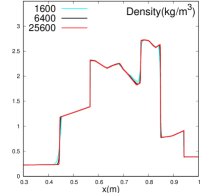
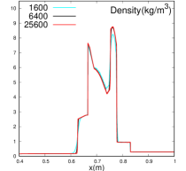
Figure 1: Density profile for the Woodward-Colella blast wave problem using the Jones-Wilkins-Lee equation of state. Left: Case 1 at $T=0.038$. Right: Case 2 at $T=$8.2\text{\times}{10}^{-4}\text{\,}$$.

The initial state for the blast wave problem is given as follows:

(5.8) $$(\rho_{0}(x),v_{0}(x),p_{0}(x))=\begin{cases}(1,0,10^{3})&\quad\text{ if }x\in[0,0.1],\\ (1,0,10^{-2})&\quad\text{ if }x\in(0.1,0.9),\\ (1,0,10^{2})&\quad\text{ if }x\in[0.9,1].\end{cases}$$

The simulations are performed on the domain $D=(0,1)$ with the TAMU code. All the tests use $\text{CFL}=0.9$ and slip boundary conditions. We show in Figure 1 the density profiles for both cases at their respective final times using three different meshes composed of $1600$, $6400$, and $25600$ elements. The results compare well with what is available in the literature; see e.g., Toro et al. [39, Fig. 2] for Case 1.

5.4.2 1D – Riemann Problem with SESAME database

We now demonstrate the method’s ability to handle tabulated data as the pressure oracle. In particular, we consider a Riemann problem modeling the impact of a right-moving aluminum slab into a stationary aluminum slab at high velocities. To simulate the material aluminum, we use the Material ID 3720 in the SESAME database [27]. We let the density of the two aluminum slabs be $\rho_{0}=$3000\text{\,}\mathrm{k}\mathrm{g}~{}\mathrm{m}^{-3}$$. The pressure at this density and at room temperature ($293\text{\,}\mathrm{K}$) is $p_{0}=$1.004\,489\text{\times}{10}^{10}\text{\,}\mathrm{P}\mathrm{a}$$ (this value is obtained from the SESAME database).

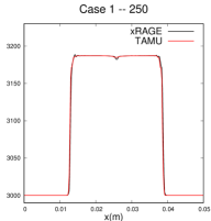
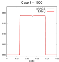
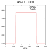
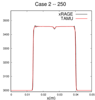
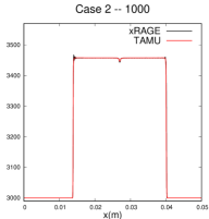
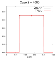
Figure 2: Density comparison for the aluminum impact problem with the TAMU and xRAGE codes using the SESAME database.

The computational domain is set to $D=(0,$0.05\text{\,}\mathrm{m}$)$ where the two aluminum slabs are separated at $x=$0.025\text{\,}\mathrm{m}$$. We consider two cases: we assume in the first case that the left slab initially moves with velocity $800\text{\,}\mathrm{m}~{}\mathrm{s}^{-1}$ (Case 1), and in the second case we assume that the velocity is $2000\text{\,}\mathrm{m}~{}\mathrm{s}^{-1}$ (Case 2). The simulations are run until final time $T=$2\text{\times}{10}^{-6}\text{\,}\mathrm{s}$$ and performed with 250, 1000 and 4000 mesh elements to show convergence. We use $\text{CFL}=0.5$ and set Dirichlet conditions on the left boundary and slip conditions on the right boundary. For verification, we run the same configuration with the xRAGE code developed at Los Alamos National Laboratory (see: [11] and [13]). In Figure 2, we show the density output comparison between the two codes.We see very good agreement between the codes. This test clearly demonstrates the method’s ability to handle tabulated data.

5.5 2D – Shock Collision with Triangular Obstacle

We now reproduce a 2D problem proposed in Toro et al. [39, Sec. 5.4] which investigates traveling shock waves colliding with a triangular obstacle. This configuration is commonly known in the literature as Schardin’s problem [36]. We refer the reader to Chang and Chang [3] where the authors experimentally reproduced Schardin’s original experiments and give a detailed description of the experiments.

This test is performed with the Van der Waals equation of state (5.2) with $\gamma=864.7/577.8,\,a=0.14,\,b=$3.258\text{\times}{10}^{-5}$$ and initialized as follows. The relative Mach speed is $M_{S}=1.3$ with the primitive state in front of the shock set to ${\bm{u}}_{R}=(1.225,0,0,101325)^{\mathsf{T}}$. Using the Rankine-Hugoniot conditions to derive the post shock state, the complete initial state is given as follows:

(5.9) $$\big{(}\rho_{0}({\bm{x}}),{\bm{v}}_{0}({\bm{x}}),p_{0}({\bm{x}})\big{)}=\begin{cases}(1.82039,148.597,0,185145),&\quad\text{ if }x\leq-0.55,\\ (1.225,0,0,101325),&\quad\text{ if }x>-0.55.\end{cases}$$

The computations are performed with the Ryuin code. The computational domain is defined as $D=(-0.65,0.5)\times(-0.5,0.5){\setminus}K$ where $K$ is the triangle formed by the vertices $(-0.2,0.0)$, $(0.1,1/6)$, and $(0.1,-1/6)$. The simulations are run until $T=$2.2\text{\times}{10}^{-3}$$ with a CFL of $0.6$. The mesh is composed of $7,347,200\text{\,}$ ${\mathbb{Q}}_{1}$-nodes. Dirichlet conditions are imposed on the left boundary, dynamic outflow conditions on the right boundary and slip conditions on the rest of the boundaries.

We show in Figure 3 the Schlieren output of the shock wave interacting with the triangular obstacle at three time snapshots $t=\{$1\text{\times}{10}^{-3}$,$1.6\text{\times}{10}^{-3}$,$2.2\text{\times}{10}^{-3}$\}$. The results match up well with the experimental photos shown in [3]. In particular, we see vortices developing along the slip layer behind the back vertices of the triangle (see: [3, Fig. 8]); these so-called vortexlets are not apparent in [39, Fig. 6] likely due to a lack of mesh resolution.

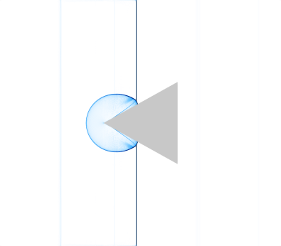
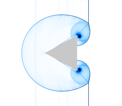
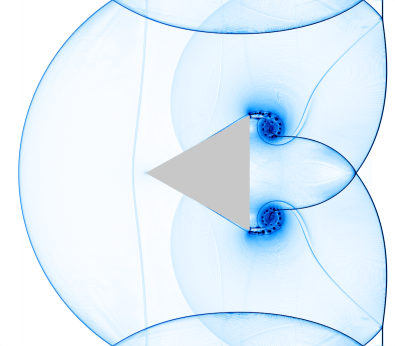
Figure 3: Shock wave interacting with triangular obstacle at $t=\{$1\text{\times}{10}^{-3}$,$1.6\text{\times}{10}^{-3}$,$2.2\text{\times}{10}^{-3}$\}$.

5.6 2D – Shock Bubble Interaction

In this section, we consider a single material shock-bubble interaction benchmark proposed in Wang and Li [40, Sec 5.2.2] using the Jones-Wilkins-Lee equation of state. For more details on shock-bubble interaction problems, we refer to Haas and Sturtevant [22] for experimental results and to Quirk and Karni [33] for the description of the simulation setup. This test demonstrates the robustness of our method by being able to reproduce the complex interactions of the shock hitting the bubble.

Let $\mathfrak{B}$ denote the bubble centered at $($0.5\text{\,}$,$0.5\text{\,}$)$ with radius $0.25\text{\,}$. The primitive states at the initial time for the ambient fluid and bubble are respectively defined as follows:

(5.10) $$(\rho_{R},{\bm{v}}_{R},p_{R}) =($1.0\text{\times}{10}^{3}\text{\,}$,$0\text{\,}$,$5.0\text{\times}{10}^{10}\text{\,}$),$$

(5.11) $$(\rho_{\mathfrak{B}},{\bm{v}}_{\mathfrak{B}},p_{\mathfrak{B}}) =($2.0\text{\times}{10}^{3}\text{\,}$,$0\text{\,}$,$5.0\text{\times}{10}^{10}\text{\,}$).$$

The pressure across the shock is prescribed to be $p_{L}=$4.369\text{\times}{10}^{11}\text{\,}$$, and the remaining state variables, $\rho_{L}$ and ${\bm{v}}_{L}$, are computed using the Rankine-Hugoniot conditions. Thus, the initial primitive state for the problem is given by

(5.12) $$(\rho_{0}({\bm{x}}),{\bm{v}}_{0}({\bm{x}}),p_{0}({\bm{x}}))=\begin{cases}(3778.85,16867.6,0,4.369\times 10^{11}),&\text{ if }x<0.05,\\ (1000,0,0,5\times 10^{10}),&\text{ if }x\geq 0.05\text{ and }{\bm{x}}\not\in\mathfrak{B},\\ (2000,0,0,5\times 10^{10}),&\text{ if }{\bm{x}}\in\mathfrak{B}.\end{cases}$$

We perform the tests with the Ryujin code. The parameters for the JWL EOS (5.4) are set to

$$A=$8.545\text{\times}{10}^{11}\text{\,}$,\,B=$2.05\text{\times}{10}^{10}\text{\,}$,\,R_{1}=4.6,\,R_{2}=1.35,\,\omega=0.25,\,\rho_{0}=$1.84\text{\times}{10}^{3}\text{\,}$.$$

The computational domain is set to $D=(0,$3\text{\,}$)\times(0,$1\text{\,}$)$ and the mesh is composed of $50,348,033\text{\,}$ ${\mathbb{Q}}_{1}$-nodes. The simulations are performed until the final time $T=$100\text{\,}\mu\mathrm{s}$$ with CFL$=0.5$. Slip boundary conditions are applied on all boundaries. In Figures 4 to 6, we show the Schlieren plots of the density at times $t=\{$40\text{\,}\mu\mathrm{s}$$, $70\text{\,}\mu\mathrm{s}$$,$100\text{\,}\mu\mathrm{s}$\}$. The results compare well with Figures 5.6 and 5.7 shown in Wang and Li [40].

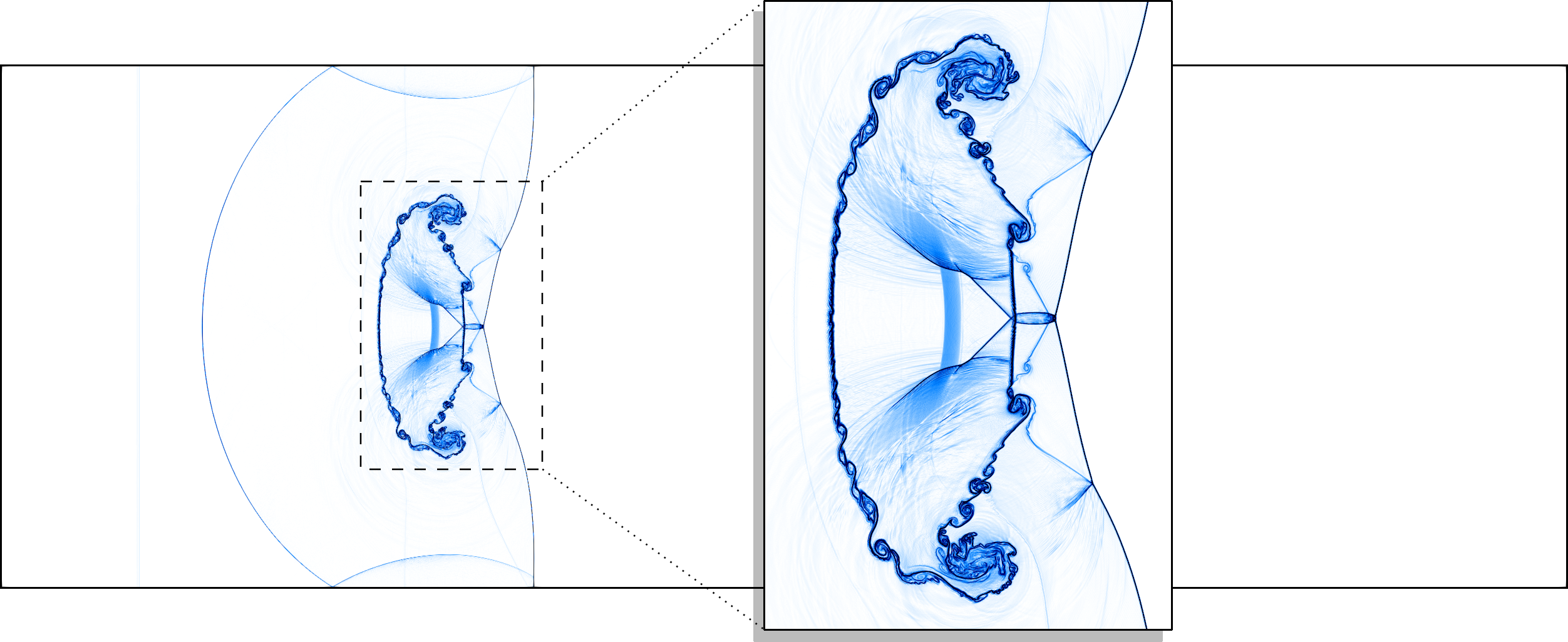
Figure 4: Schlieren plots for the shock-bubble interaction benchmark for $t=$40\text{\,}\mu\mathrm{s}$$.

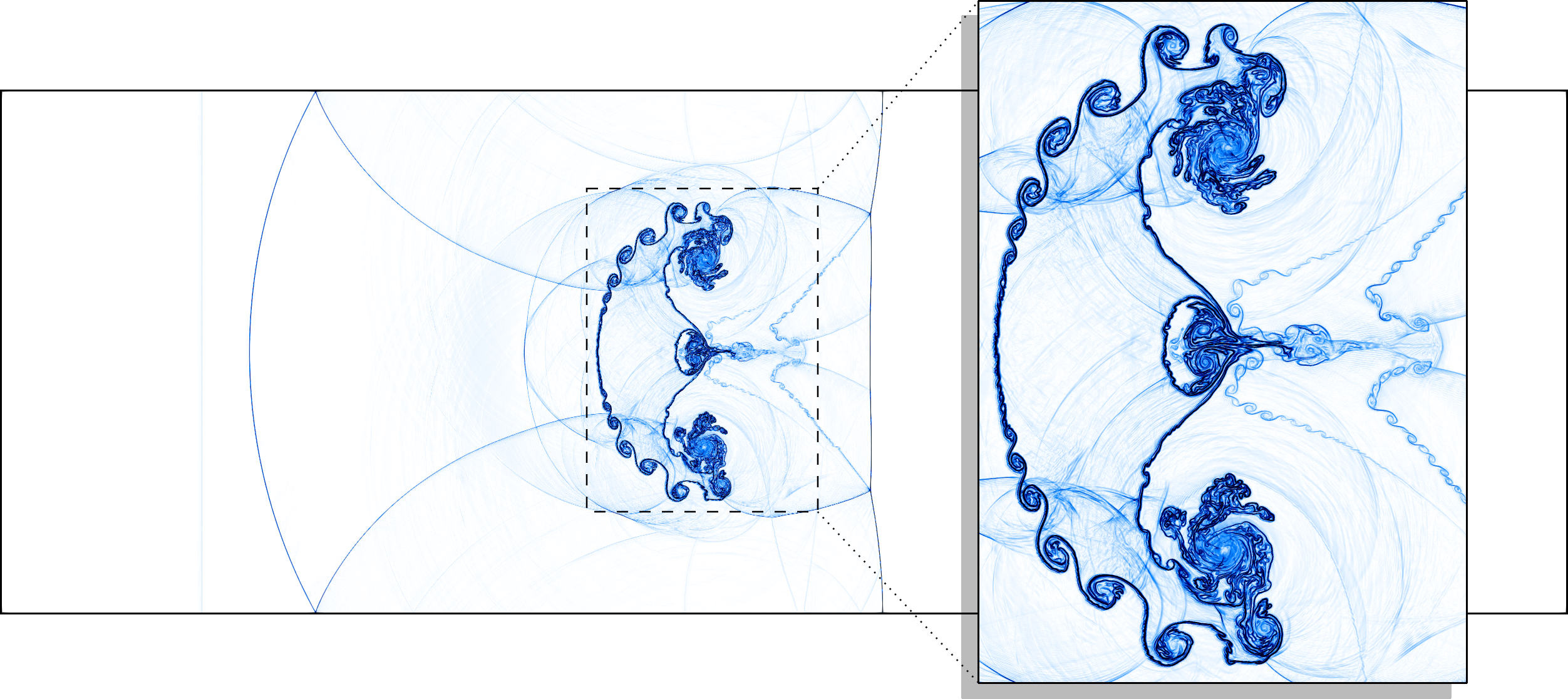
Figure 5: Schlieren plots for the shock-bubble interaction benchmark for $t=$70\text{\,}\mu\mathrm{s}$$.

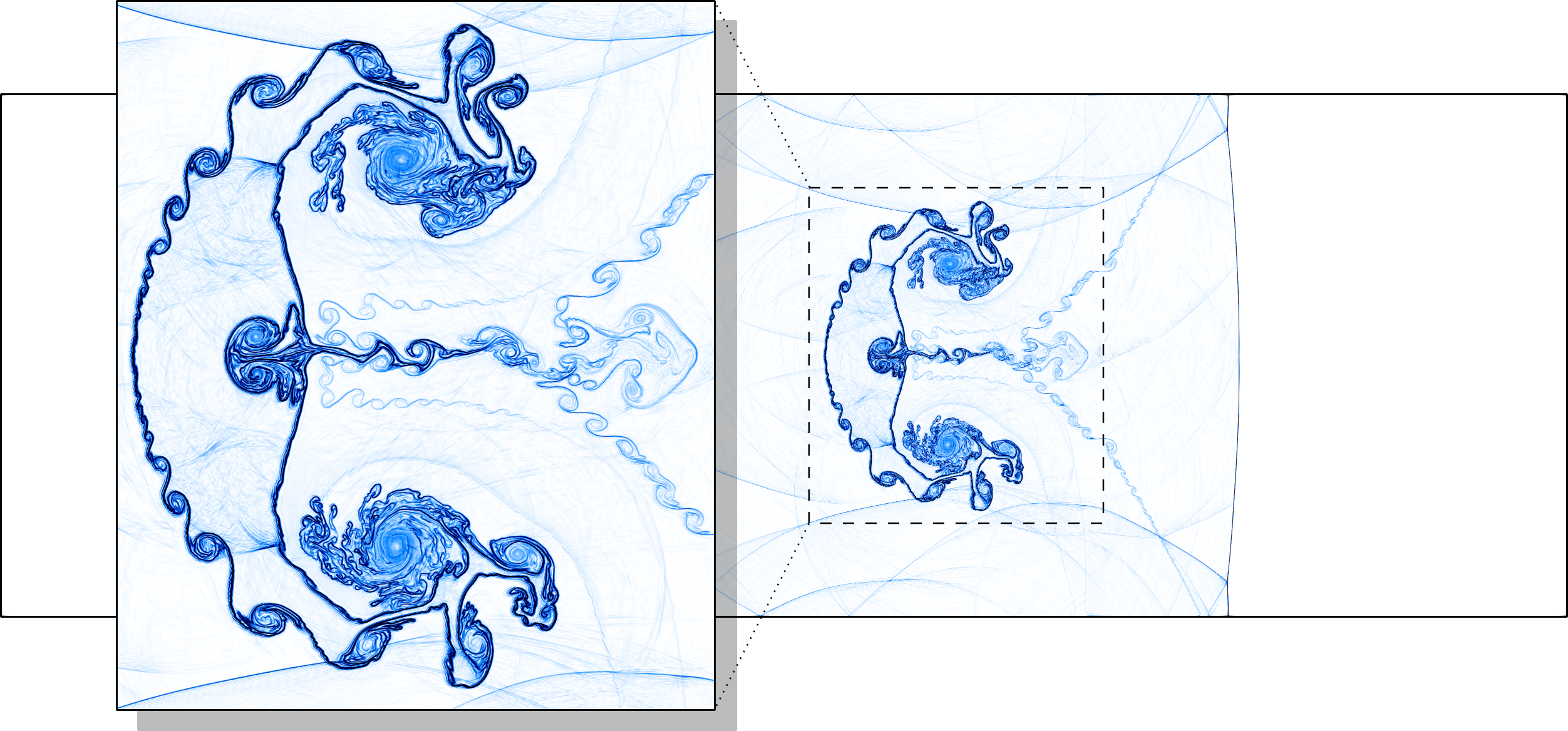
Figure 6: Schlieren plots for the shock-bubble interaction benchmark for $t=$100\text{\,}\mu\mathrm{s}$$ (bottom).

6 Conclusion

We have developed an invariant-domain preserving second-order accurate method for the Euler equations with arbitrary or tabulated equation of states. The work presented is the continuation and extension of Guermond et al. [18] and Clayton et al. [6]. We proposed a surrogate entropy functional that increases across shocks in the associated 1D Riemann problem to work around the lack of a general mathematical entropy valid for arbitrary equations of state. A convex limiting procedure was performed on this surrogate entropy functional to enforce a local minimum principle. This in turn implies a positive local lower bound on the internal energy. Numerical evidence of higher order accuracy was demonstrated with convergence tests and several computational benchmarks.

Appendix A Isentropic vortex with van der Waals equation of state

We present a derivation of the isentropic vortex solution with the van der Waals equation of state and give some necessary conditions for the existence of this solution.

Theorem A.1.

Consider the van der Waals equation of state (5.2) with $a>0$, $b:=0$, and $\gamma:=\frac{3}{2}$ or $\gamma:=2$. Let ${\bm{x}}^{0}\in{\mathbb{R}}^{2}$, $\beta>0$, $r_{0}>0$. Let $\rho_{\infty}>0$, ${\bm{v}}_{\infty}\in{\mathbb{R}}^{2}$, $p_{\infty}>0$ and assume that

(A.1) $$p_{\infty}>\tfrac{1}{3}a\rho_{\infty}^{2},\qquad a\rho_{\infty}+\frac{3p_{\infty}}{\rho_{\infty}}>\frac{\beta^{2}e^{1}}{8r_{0}^{2}\pi^{2}}$$

if $\gamma=\tfrac{3}{2}$. The following density, velocity, and pressure fields solve the compressible Euler equations (2.1a)–(2.1c) with the van der Waals equation of state:

(A.2a) $$\rho({\bm{x}},t) :=\begin{cases}\Big{(}\tfrac{3C}{4a}-\tfrac{1}{2}\sqrt{\tfrac{9C^{2}}{4a^{2}}+\tfrac{2}{a}\big{(}F+\tfrac{1}{2r_{0}^{2}}\psi(\overline{{\bm{x}}})^{2}\big{)}}\Big{)}^{2},&\;\text{ if }\gamma=\tfrac{3}{2},\\ \rho_{\infty}-\frac{\rho^{2}_{\infty}}{4p_{\infty}r_{0}^{2}}\psi(\overline{{\bm{x}}}),&\;\text{ if }\gamma=2,\end{cases}$$

(A.2b) $${\bm{v}}({\bm{x}},t) :={\bm{v}}_{\infty}+\psi(\overline{{\bm{x}}})(-\bar{x}_{2},\bar{x}_{1})^{\mathsf{T}},$$

(A.2c) $$p({\bm{x}},t) :=C\rho({\bm{x}},t)^{\gamma}-a\rho({\bm{x}},t)^{2},$$

with $\psi(\overline{{\bm{x}}}):=\tfrac{\beta}{2\pi}\exp(\tfrac{1}{2}(1-\tfrac{1}{r_{0}^{2}}\|\overline{{\bm{x}}}\|^{2}_{\ell^{2}}))$, $(\bar{x}_{1},\bar{x}_{2})=\overline{{\bm{x}}}:={\bm{x}}-{\bm{x}}^{0}-{\bm{v}}_{\infty}t$, $C=(p_{\infty}+a\rho_{\infty}^{2})/\rho_{\infty}^{3/2}$, and $F=-a\rho_{\infty}-3p_{\infty}/\rho_{\infty}$. $\square$

Proof A.2.

The derivation of the isentropic vortex begins with the additional assumption that the velocity field is divergence free. That is, $\nabla{\cdot}{\bm{v}}=0$. Under this assumption the Euler equations take the following simplified form:

(A.3) $$\partial_{t}\rho({\bm{x}},t)+{\bm{v}}({\bm{x}},t){\cdot}\nabla\rho({\bm{x}},t) =0, \quad{\bm{x}}\in\mathbb{R}^{2},\,t>0,$$

(A.4) $$\partial_{t}{\bm{v}}({\bm{x}},t)+({\bm{v}}({\bm{x}},t){\cdot}\nabla){\bm{v}}({\bm{x}},t) =-\frac{1}{\rho({\bm{x}},t)}\nabla p({\bm{x}},t), \quad{\bm{x}}\in\mathbb{R}^{2},\,t>0$$

(A.5) $$\partial_{t}e({\bm{x}},t)+{\bm{v}}({\bm{x}},t){\cdot}\nabla e({\bm{x}},t) =0, \quad{\bm{x}}\in\mathbb{R}^{2},\,t>0,$$

with ${\bm{x}}:=(x_{1},x_{2})$, boundary conditions, $(\rho_{\infty},{\bm{v}}_{\infty}{:=}(v_{1,\infty},v_{2,\infty})^{\mathsf{T}},p_{\infty})$ and yet to be determined initial conditions $(\rho_{0}({\bm{x}}),{\bm{v}}_{0}({\bm{x}}),p_{0}({\bm{x}}))$. To keep things general, we make no assumption on the equation of state for $p=p(\rho,e)$.

We write the solution as a perturbation of the far-field state; i.e., we define ${\bm{v}}:={\bm{v}}_{\infty}+\delta{\bm{v}}$ with

(A.6) $$\delta{\bm{v}}({\bm{x}},t):=\begin{pmatrix}\partial_{x_{2}}\psi({\bm{x}}-{\bm{x}}^{0}-{\bm{v}}_{\infty}t)\\ -\partial_{x_{1}}\psi({\bm{x}}-{\bm{x}}^{0}-{\bm{v}}_{\infty}t)\end{pmatrix},$$

with the stream function $\psi({\bm{x}}):=\frac{\beta}{2\pi}\exp(\tfrac{1}{2}(1-\tfrac{\|{\bm{x}}\|_{\ell^{2}}^{2}}{r_{0}^{2}}))$. Here ${\bm{x}}^{0}:=(x_{1}^{0},x_{2}^{0})\in\mathbb{R}^{2}$, $\beta$, and $r_{0}$ are free parameters. To further simplify notation, define $(\bar{x}_{1},\bar{x}_{2})=\overline{{\bm{x}}}:={\bm{x}}-{\bm{x}}^{0}-{\bm{v}}_{\infty}t$ and $r^{2}:=\|\overline{{\bm{x}}}\|_{\ell^{2}}^{2}$. Note the following identities which will be used later on:

(A.7) $$\partial_{x_{i}}\psi(\overline{{\bm{x}}}) =-\frac{\bar{x}_{i}}{r_{0}^{2}}\psi(\overline{{\bm{x}}}),$$

(A.8) $$\partial_{x_{i}x_{j}}\psi(\overline{{\bm{x}}}) =\frac{1}{r_{0}^{2}}\Big{(}-\delta_{ij}+\frac{\bar{x}_{i}\bar{x}_{j}}{r_{0}^{2}}\Big{)}\psi(\overline{{\bm{x}}}),$$

(A.9) $$\partial_{tx_{i}}\psi(\overline{{\bm{x}}}) =\frac{1}{r_{0}^{2}}\Big{(}v_{i,\infty}-\frac{\bar{x}_{i}{\bm{v}}_{\infty}\cdot\overline{{\bm{x}}}}{r_{0}^{2}}\Big{)}\psi(\overline{{\bm{x}}}),$$

where $\delta_{ij}$ is the Kronecker symbol and $i,j\in\{1,2\}$.

Using that ${\bm{v}}={\bm{v}}_{\infty}+\delta{\bm{v}}$, the left hand side of (A.4) becomes,

(A.10) $$\partial_{t}{\bm{v}}+{\bm{v}}\cdot\nabla{\bm{v}}=\partial_{t}(\delta{\bm{v}})+({\bm{v}}_{\infty}\cdot\nabla)\delta{\bm{v}}+(\delta{\bm{v}}\cdot\nabla)\delta{\bm{v}}.$$

From the definition of $\delta{\bm{v}}$ and the identities (A.7), (A.8) and (A.9), we have,

(A.11) $$(\delta{\bm{v}}\cdot\nabla)\delta{\bm{v}} =\begin{bmatrix}(\partial_{x_{2}}\psi)(\partial^{2}_{x_{1}x_{2}}\psi)-(\partial_{x_{1}}\psi)(\partial^{2}_{x_{2}}\psi)\\ -(\partial_{x_{2}}\psi)(\partial^{2}_{x_{1}}\psi)+(\partial_{x_{1}}\psi)(\partial^{2}_{x_{1}x_{2}}\psi)\end{bmatrix}=-\frac{\overline{{\bm{x}}}}{r_{0}^{4}}\psi(\overline{{\bm{x}}})^{2}$$

(A.12) $$({\bm{v}}_{\infty}\cdot\nabla)\delta{\bm{v}} =\frac{1}{r_{0}^{2}}\Big{(}-\begin{bmatrix}v_{2,\infty}\\ -v_{1,\infty}\end{bmatrix}+\frac{{\bm{v}}_{\infty}\cdot\overline{{\bm{x}}}}{r_{0}^{2}}\begin{bmatrix}\bar{x}_{2}\\ -\bar{x}_{1}\end{bmatrix}\Big{)}\psi(\overline{{\bm{x}}})$$

(A.13) $$\partial_{t}(\delta{\bm{v}}) =\frac{1}{r_{0}^{2}}\Big{(}\begin{bmatrix}v_{2,\infty}\\ -v_{1,\infty}\end{bmatrix}-\frac{{\bm{v}}_{\infty}\cdot\overline{{\bm{x}}}}{r_{0}^{2}}\begin{bmatrix}\bar{x}_{2}\\ -\bar{x}_{1}\end{bmatrix}\Big{)}\psi(\overline{{\bm{x}}})$$

Thus equation (A.4) becomes $-\frac{\overline{{\bm{x}}}}{r_{0}^{4}}\psi(\overline{{\bm{x}}})^{2}=-\frac{1}{\rho}\nabla p$. This identity is furthermore written as,

(A.14) $$-\frac{1}{2r_{0}^{2}}\nabla(\psi(\overline{{\bm{x}}})^{2})=\frac{1}{\rho(t,{\bm{x}})}\nabla p(\rho(t,{\bm{x}})).$$

Up to this point, we have not made any assumption on the equation of state. We recover the well known isentropic vortex solution if we assume the pressure is given by the ideal gas law; i.e., $p(\rho)=C\rho^{\gamma}$ for the isentropic flow where $C=p_{\infty}/\rho_{\infty}^{\gamma}$. We now proceed with the van der Waals equation of state. For isentropic flows we have

(A.15) $$p(\rho)=\frac{C\rho^{\gamma}}{(1-b\rho)^{\gamma}}-a\rho^{2},$$

where $C$ is some constant. (Note, we work with an arbitrary $b$ to keep things general in the beginning.) Following the same process as in the ideal gas case, we compute the indefinite integral, $\int\frac{1}{\rho}\partial_{x_{i}}p(\rho)\>dx_{i}$:

$$-\frac{1}{2r_{0}^{2}}\int\partial_{x_{i}}\psi(\overline{\bm{x}})^{2}\>dx_{i}=\int\frac{1}{\rho}\partial_{x_{i}}p(\rho)\>dx_{i}=\frac{p(\rho)}{\rho}+\int\frac{p(\rho)}{\rho^{2}}\partial_{x_{i}}\rho\>dx_{i}\\ =\frac{p(\rho)}{\rho}+\int\Big{(}\frac{C\rho^{\gamma-2}}{(1-b\rho)^{\gamma}}-a\Big{)}\rho_{x_{i}}dx_{i}=\frac{p(\rho)}{\rho}+\int\frac{\partial}{\partial x_{i}}\Big{[}\frac{C}{\gamma-1}\Big{(}\frac{\rho}{1-b\rho}\Big{)}^{\gamma-1}-a\rho\Big{]}\>dx_{i}\\ =\frac{C\rho^{\gamma-1}(\gamma-b\rho)}{(\gamma-1)(1-b\rho)^{\gamma}}-2a\rho+F.$$

Hence, $\rho(\overline{\bm{x}})$ can be found by solving the equation,

(A.16) $$-\frac{1}{2r_{0}^{2}}\psi(\overline{{\bm{x}}})^{2}=\frac{C\rho^{\gamma-1}(\gamma-b\rho)}{(\gamma-1)(1-b\rho)^{\gamma}}-2a\rho+F.$$

We have two immediate cases for solutions that can be found explicitly.

Case 1: $\gamma=3/2$ and $b=0$: In this case, (A.16) becomes a quadratic equation for $\sqrt{\rho}$,

(A.17) $$\rho-\frac{3C}{2a}\sqrt{\rho}-\frac{1}{2a}\Big{(}F+\frac{1}{2r_{0}^{2}}\psi(\overline{{\bm{x}}})^{2}\Big{)}=0.$$

The constants $C$ and $F$ are determined by applying the far field condition to (A.15) and (A.17):

(A.18) $$C=\frac{p_{\infty}+a\rho_{\infty}^{2}}{\rho^{3/2}_{\infty}}\quad\text{and}\quad F=-a\rho_{\infty}-\frac{3p_{\infty}}{\rho_{\infty}}.$$

However, care must be taken in the choice of $p_{\infty}$ and $\rho_{\infty}$ so that the sound speed remains real. Recall that the sound speed for the van der Waals EOS is $c(\rho,p)=\sqrt{\gamma\frac{p+a\rho^{2}}{\rho(1-b\rho)}-2a\rho}$. The hypothesis $p_{\infty}>\frac{1}{3}a\rho_{\infty}^{2}$ guarantees that $c(\rho_{\infty},p_{\infty})^{2}>0$.

The physical root for equation (A.17) is $\sqrt{\rho}=\tfrac{3C}{4a}-\tfrac{1}{2}\sqrt{\tfrac{9C^{2}}{4a^{2}}+\tfrac{2}{a}\big{(}F+\tfrac{1}{2r_{0}^{2}}\psi(\overline{{\bm{x}}})^{2}\big{)}}$. Furthermore, for the root to be real we require that $-F>\frac{1}{2r_{0}^{2}}\psi(\overline{{\bm{x}}})^{2}$ for all $\overline{{\bm{x}}}\in\mathbb{R}^{2}$. In particular,

(A.19) $$a\rho_{\infty}+\frac{3p_{\infty}}{\rho_{\infty}}>\frac{\beta^{2}e^{1}}{8r_{0}^{2}\pi^{2}}.$$

Lastly, we must justify that the system remains hyperbolic; that is, the sound speed is real for all $({\bm{x}},t)\in{\mathbb{R}}^{2}{\times}[0,\infty)$. Since the flow is isentropic, the sound speed for the van der Waals EOS (with $\gamma=3/2$ and $b=0$) is, $f(\rho):=c(p(\rho),\rho)^{2}=\frac{3}{2}C\sqrt{\rho}-2a\rho$. Note that $\lim_{\rho\to 0^{+}}f(\rho)=0$, $f^{\prime}(\rho)=\frac{3C}{4\sqrt{\rho}}-2a$, and $\lim_{\rho\to 0^{+}}f^{\prime}(\rho)=\infty$. Therefore, $f(\rho)$ has a maximum at $\rho=\big{(}\frac{3C}{8a}\big{)}^{2}$ and hence $f(\rho)>0$ for $\rho\in(0,\big{(}\frac{3C}{8a}\big{)}^{2})$. From the definition of $\rho$, (A.2a), we see that $0<\rho<\big{(}\frac{3C}{4a}\big{)}^{2}$. Thus the sound speed is always real.

Case 2: $\gamma=2$ and $b=0$: For these choices of parameters, (A.16) becomes,

(A.20) $$2(C-a)\rho+F+\frac{1}{2r_{0}^{2}}\psi(\overline{{\bm{x}}})=0.$$

Using the far field boundary conditions for (A.2c) and (A.20) we find that $C=\frac{p_{\infty}}{\rho^{2}_{\infty}}+a$ and $F=-2p_{\infty}/\rho_{\infty}$, respectively. Solving for $\rho$ in (A.20) we have,

(A.21) $$\rho=\rho_{\infty}-\frac{\rho^{2}_{\infty}}{4p_{\infty}r_{0}^{2}}\psi(\overline{{\bm{x}}}).$$

Note the sound speed is $c(p(\rho),\rho)^{2}=2(C-a)\rho=\frac{2p_{\infty}}{\rho_{\infty}}\rho>0$. $\square$

References

- Banks [2010] J. W. Banks. On exact conservation for the Euler equations with complex equations of state. Communications in Computational Physics, 8:995–1015, 2010.
- Banks et al. [2008] J. W. Banks, W. D. Henshaw, D. W. Schwendeman, and A. K. Kapila. A study of detonation propagation and diffraction with compliant confinement. Combustion Theory and Modelling, 12(4):769–808, 2008. 10.1080/13647830802123564. URL https://doi.org/10.1080/13647830802123564.
- Chang and Chang [2000] S.-M. Chang and K.-S. Chang. On the shock–vortex interaction in schardin’s problem. Shock Waves, 10(5):333–343, 2000.
- Christon et al. [2004] M. A. Christon, M. J. Martinez, and T. E. Voth. Generalized Fourier analyses of the advection-diffusion equation-part I: one-dimensional domains. International Journal for Numerical Methods in Fluids, 45(8):839–887, 2004.
- Clayton et al. [2021] B. Clayton, J.-L. Guermond, and B. Popov. Upper bound on the maximum wave speed in riemann problems for the Euler equations with tabulated equation of state, April 2021. URL https://doi.org/10.5281/zenodo.4685868.
- Clayton et al. [2022] B. Clayton, J.-L. Guermond, and B. Popov. Invariant domain-preserving approximations for the Euler equations with tabulated equation of state. SIAM Journal on Scientific Computing, 44(1):A444–A470, 2022.
- Colella and Glaz [1985] P. Colella and H. M. Glaz. Efficient solution algorithms for the Riemann problem for real gases. J. Comput. Phys., 59(2):264–289, 1985.
- Dukowicz [1985] J. K. Dukowicz. A general, noniterative Riemann solver for Godunov’s method. J. Comput. Phys., 61(1):119–137, 1985.
- Dumbser and Casulli [2016] M. Dumbser and V. Casulli. A conservative, weakly nonlinear semi-implicit finite volume scheme for the compressible Navier-Stokes equations with general equation of state. Appl. Math. Comput., 272(part 2):479–497, 2016.
- Dumbser et al. [2013] M. Dumbser, U. Iben, and C.-D. Munz. Efficient implementation of high order unstructured weno schemes for cavitating flows. Computers & Fluids, 86:141–168, 2013.
- Gittings et al. [2008] M. Gittings, R. Weaver, M. Clover, T. Betlach, N. Byrne, R. Coker, E. Dendy, R. Hueckstaedt, K. New, W. R. Oakes, D. Ranta, and R. Stefan. The RAGE radiation-hydrodynamic code. Computational Science & Discovery, 1(1):015005, Nov 2008.
- Godlewski and Raviart [1996] E. Godlewski and P.-A. Raviart. Numerical approximation of hyperbolic systems of conservation laws, volume 118 of Applied Mathematical Sciences. Springer-Verlag, New York, 1996.
- Grove [2019] J. W. Grove. The xrage hydrodynamic solver. Technical report, 2019. URL https://www.osti.gov/biblio/1532686.
- Guermond and Pasquetti [2013] J.-L. Guermond and R. Pasquetti. A correction technique for the dispersive effects of mass lumping for transport problems. Comput. Methods Appl. Mech. Engrg., 253:186–198, 2013.
- Guermond and Popov [2016a] J.-L. Guermond and B. Popov. Fast estimation from above of the maximum wave speed in the Riemann problem for the Euler equations. J. Comput. Phys., 321:908–926, 2016a.
- Guermond and Popov [2016b] J.-L. Guermond and B. Popov. Invariant domains and first-order continuous finite element approximation for hyperbolic systems. SIAM J. Numer. Anal., 54(4):2466–2489, 2016b.
- Guermond et al. [2011] J.-L. Guermond, R. Pasquetti, and B. Popov. Entropy viscosity method for nonlinear conservation laws. J. Comput. Phys., 230(11):4248–4267, 2011.
- Guermond et al. [2018] J.-L. Guermond, M. Nazarov, B. Popov, and I. Tomas. Second-order invariant domain preserving approximation of the Euler equations using convex limiting. SIAM J. Sci. Comput., 40(5):A3211–A3239, 2018.
- Guermond et al. [2019] J.-L. Guermond, B. Popov, and I. Tomas. Invariant domain preserving discretization-independent schemes and convex limiting for hyperbolic systems. Comput. Methods Appl. Mech. Engrg., 347:143–175, 2019.
- Guermond et al. [2021] J.-L. Guermond, M. Maier, B. Popov, and I. Tomas. Second-order invariant domain preserving approximation of the compressible Navier-Stokes equations. Computer Methods in Applied Mechanics and Engineering, 375(1):113608, 2021.
- Guermond et al. [2022] J.-L. Guermond, M. Kronbichler, M. Maier, B. Popov, and I. Tomas. On the implementation of a robust and efficient finite element-based parallel solver for the compressible Navier–Stokes equations. Computer Methods in Applied Mechanics and Engineering, 389:114250, 2022.
- Haas and Sturtevant [1987] J.-F. Haas and B. Sturtevant. Interaction of weak shock waves with cylindrical and spherical gas inhomogeneities. Journal of Fluid Mechanics, 181:41–76, 1987.
- Ivings et al. [1998] M. J. Ivings, D. M. Causon, and E. F. Toro. On Riemann solvers for compressible liquids. Internat. J. Numer. Methods Fluids, 28(3):395–418, 1998.
- Lax [1954] P. D. Lax. Weak solutions of nonlinear hyperbolic equations and their numerical computation. Comm. Pure Appl. Math., 7:159–193, 1954.
- Lee et al. [2013] B. J. Lee, E. F. Toro, C. E. Castro, and N. Nikiforakis. Adaptive osher-type scheme for the Euler equations with highly nonlinear equations of state. Journal of Computational Physics, 246:165–183, 2013.
- Lee et al. [1968] E. L. Lee, H. C. Hornig, and J. W. Kury. Adiabatic expansion of high explosive detonation products. Technical Report UCRL-50422, Lawrence Radiation Laboratory, University of California, Livermore, May 2 1968. URL https://www.osti.gov/biblio/4783904.
- Lyon [1992] S. P. Lyon. SESAME: The Los Alamos National Laboratory equation of state database. Los Alamos National Laboratory report LA-UR-92-3407, 1992.
- Maier and Kronbichler [2021] M. Maier and M. Kronbichler. Efficient parallel 3d computation of the compressible Euler equations with an invariant-domain preserving second-order finite-element scheme. ACM Transactions on Parallel Computing, 8(3):16:1–30, 2021.
- Menikoff [2007] R. Menikoff. Empirical Equations of State for Solids, pages 143–188. Springer Berlin Heidelberg, 2007. 10.1007/978-3-540-68408-4_4.
- Persson and Peraire [2006] P.-O. Persson and J. Peraire. Sub-cell shock capturing for discontinuous galerkin methods. In 44th AIAA Aerospace Sciences Meeting and Exhibit, number AIAA paper no. 2015-2006-112 in Aerospace Sciences Meetings, 2006.
- Pike [1993] J. Pike. Riemann solvers for perfect and near-perfect gases. AIAA Journal, 31(10):1801–1808, 1993.
- Quartapelle et al. [2003] L. Quartapelle, L. Castelletti, A. Guardone, and G. Quaranta. Solution of the Riemann problem of classical gasdynamics. J. Comput. Phys., 190(1):118–140, 2003.
- Quirk and Karni [1996] J. J. Quirk and S. Karni. On the dynamics of a shock-bubble interaction. Journal of Fluid Mechanics, 318:129–163, 1996.
- Roe and Pike [1985] P. L. Roe and J. Pike. Efficient construction and utilisation of approximate riemann solutions. In Proceedings of the Sixth International Symposium on Computing Methods in Applied Sciences and Engineering, VI, pages 499–518, Netherlands, 1985. North-Holland Publishing Co.
- Saurel et al. [2007] R. Saurel, E. Franquet, E. Daniel, and O. Le Metayer. A relaxation-projection method for compressible flows. part i: The numerical equation of state for the Euler equations. Journal of Computational Physics, 223(2):822–845, 2007.
- Schardin [1957] H. Schardin. High frequency cinematography in the shock tube. The Journal of Photographic Science, 5(2):17–19, 1957.
- Segletes [2018] S. B. Segletes. An examination of the JWL equation of state. Technical Report AD1055483, Army Research Lab Aberdeen Proving Ground, MD, United States, 2018.
- Thompson [2016] T. Thompson. A discrete commutator theory for the consistency and phase error analysis of semi-discrete finite element approximations to the linear transport equation. J. Comput. Appl. Math., 303:229–248, 2016.
- Toro et al. [2015] E. F. Toro, C. E. Castro, and B. J. Lee. A novel numerical flux for the 3D Euler equations with general equation of state. J. Comput. Phys., 303:80–94, 2015.
- Wang and Li [2021] Y. Wang and J. Li. Stiffened gas approximation and grp resolution for fluid flows of real materials. arXiv preprint, arXiv:2108.13780, 2021.
- Yee et al. [1999] H. Yee, N. Sandham, and M. Djomehri. Low-dissipative high-order shock-capturing methods using characteristic-based filters. Journal of Computational Physics, 150(1):199–238, 1999.