Large-Scale Low-Rank Gaussian Process Prediction with Support Points

Abstract

Low-rank approximation is a popular strategy to tackle the “big $n$ problem” associated with large-scale Gaussian process regressions. Basis functions for developing low-rank structures are crucial and should be carefully specified. Predictive processes simplify the problem by inducing basis functions with a covariance function and a set of knots. The existing literature suggests certain practical implementations of knot selection and covariance estimation; however, theoretical foundations explaining the influence of these two factors on predictive processes are lacking. In this paper, the asymptotic prediction performance of the predictive process and Gaussian process predictions is derived and the impacts of the selected knots and estimated covariance are studied. We suggest the use of support points as knots, which best represent data locations. Extensive simulation studies demonstrate the superiority of support points and verify our theoretical results. Real data of precipitation and ozone are used as examples, and the efficiency of our method over other widely used low-rank approximation methods is verified.

Keywords: Convergence rate; Kernel ridge regression; Kriging; Nyström approximation; Predictive process; Spatial statistics.

1 Introduction

Gaussian processes (GPs; Rasmussen and Williams, 2006) are extensively used for solving regression problems in many fields such as spatial statistics (Stein, 1999; Gelfand et al., 2010; Cressie, 2015), computer experiments (Sacks et al., 1989; Santner et al., 2003), and machine learning (Rasmussen and Williams, 2006; Liu et al., 2020). The underlying regression function is assumed to be a realization of a GP, whose mean trend and covariance function must be evaluated. Using the conditional multivariate normal distribution, a GP provides each location with a closed-form prediction as well as a confidence interval.

Assume that a dataset $D=\{(\mathbf{x}_{i},y_{i})\}_{i=1}^{n}$ satisfies the GP model, i.e.,

$$y_{i}=f(\mathbf{x}_{i})+\epsilon_{i},\quad i=1,\ldots,n,$$ (1)

where $\mathbf{x}_{i}\in\mathcal{X}\subset\mathbb{R}^{d}$ and follows a distribution $F_{\mathbf{x}}$. The $f(\mathbf{x}_{i})$’s are the realization of a Gaussian process $Z(\cdot)$ on locations $\{\mathbf{x}_{i}\}_{i=1}^{n}$, and the nugget effects $\epsilon_{i}$’s are independent and follow a $\mathcal{N}(0,\tau^{2})$ distribution. Under the GP regression, $f$ is considered as a random function and is not distinguished from $Z$. Without considering a mean trend, we assume that $Z(\cdot)\sim\mathrm{GP}(0,c)$, where $c(\cdot,\cdot)$ is a positive definite covariance function. Then, the response vector $\mathbf{y}=(y_{1},\ldots,y_{n})^{\top}$ follows a multivariate normal distribution $\mathcal{N}_{n}(\mathbf{0},\mathbf{C}+\tau^{2}\mathbf{I}_{n})$, where $\mathbf{C}=\{c(\mathbf{x}_{i},\mathbf{x}_{j})\}_{i,j=1}^{n}$. The covariance function $c$ is usually unknown in practice and is represented by a specific parametric form $c(\cdot,\cdot;\bm{\theta})$, where the parameter vector $\bm{\theta}$ can be obtained by maximizing the likelihood function with respect to $\bm{\theta}$:

$$(2\pi)^{-n/2}|\mathbf{C}(\bm{\theta})+\tau^{2}\mathbf{I}_{n}|^{-1/2}\exp\left[-\frac{1}{2}\mathbf{y}^{\top}\{\mathbf{C}(\bm{\theta})+\tau^{2}\mathbf{I}_{n}\}^{-1}\mathbf{y}\right].$$

With the conditional probability density of the multivariate normal distribution, the prediction based on $c$ at any $\mathbf{x}\in\mathcal{X}$ is

$$\hat{f}_{c}(\mathbf{x})=\mathbf{c}(\mathbf{x})^{\top}(\mathbf{C}+\tau^{2}\mathbf{I}_{n})^{-1}\mathbf{y},$$ (2)

where $\mathbf{c}(\mathbf{x})=\{c(\mathbf{x},\mathbf{x}_{1}),\ldots,c(\mathbf{x},\mathbf{x}_{n})\}^{\top}$. Fitting data of size $n$ with a GP requires $O(n^{3})$ operations and $O(n^{2})$ memory, and these requirements may easily exhaust computational resources even with a moderately large $n$.

Many methods are available to tackle the challenge of handling massive datasets with GPs. We refer the readers to Heaton et al. (2019) and Liu et al. (2020) for their comprehensive reviews. The methods of likelihood approximation include the Vecchia approximation (Vecchia, 1988; Stein et al., 2004; Katzfuss et al., 2020; Katzfuss and Guinness, 2021; Katzfuss et al., 2022), composite likelihood (Varin et al., 2011; Eidsvik et al., 2014), and hierarchical low-rank approximation (Huang and Sun, 2018). Covariance tapering multiplies the covariance function with a compactly supported one such that the tapered covariance matrix is sparse and can be solved easily (Furrer et al., 2006; Kaufman et al., 2008; Stein, 2013). Rue and Tjelmeland (2002), Rue and Held (2005), and Xu et al. (2015) discussed the methods of Markov random field approximation, which are primarily used for lattice data. Methods based on distributed computing (Paciorek et al., 2015; Deisenroth and Ng, 2015; Katzfuss and Hammerling, 2017; Abdulah et al., 2018a, b, 2019), resampling (Liang et al., 2013; Barbian and Assunção, 2017), and exact approaches using the ExaGeoStat software (Abdulah et al., 2018a) were recently proposed.

The low-rank approximation is another important approach for GPs with massive data. It approximates the original GP of mean zero with a low-rank one, which is represented by a linear combination of specified basis functions with random weights, e.g., the fixed-rank kriging (FRK, Cressie and Johannesson, 2008; Zammit-Mangion and Cressie, 2021), LatticeKrig (Nychka et al., 2015), and predictive processes (Banerjee et al., 2008; Finley et al., 2009). Combining low-rank approximations with the concept of covariance tapering can help develop multiple efficient methods (Sang and Huang, 2012; Katzfuss, 2017; Zhang et al., 2019). In this context, the choice of the basis functions is important to the performance of these methods. FRK and LatticeKrig suggest multiresolution bases to capture information at different scales. The construction of basis functions involves the delicate selections of multiple tuning parameters, such as the types of basis functions, levels of resolution, and information in the coarsest resolution (Zammit-Mangion and Cressie, 2021; Nychka et al., 2016). Tzeng and Huang (2018) proposed adaptive basis functions to avoid the manual allocation of scales.

Predictive processes simplify the aforementioned problem by developing basis functions with a covariance function and a set of specified knots. In this context, the covariance estimation and knot configuration are of particular interest. Specifically, Banerjee et al. (2008) selected a set of knots $D_{k}^{*}=\{\mathbf{x}_{i}^{*}\}_{i=1}^{k}$ well dispersed over $\mathcal{X}$, which may or may not belong to $\{\mathbf{x}_{i}\}_{i=1}^{n}$. Then, they projected the original process $Z$ onto a linear space spanned by $\mathbf{z}^{*}=\{Z(\mathbf{x}_{1}^{*}),\ldots,Z(\mathbf{x}_{k}^{*})\}^{\top}$ and induced the predictive process $\tilde{Z}(\mathbf{x})=\mathbb{E}\{Z(\mathbf{x})|\mathbf{z}^{*}\}=\mathbf{c}^{*}(\mathbf{x})^{\top}\mathbf{C}^{*-1}\mathbf{z}^{*}$, where $\mathbf{c}^{*}(\mathbf{x})=\{c(\mathbf{x},\mathbf{x}_{1}^{*}),\ldots,c(\mathbf{x},\mathbf{x}_{k}^{*})\}^{\top}$ and $\mathbf{C}^{*}=\{\mathbf{c}^{*}(\mathbf{x}_{1}^{*}),\ldots,\mathbf{c}^{*}(\mathbf{x}_{k}^{*})\}$. Correspondingly, the process $\tilde{Z}\sim\mathrm{GP}(0,\tilde{c})$, where $\tilde{c}(\mathbf{x}_{i},\mathbf{x}_{j})=\mathbf{c}^{*}(\mathbf{x}_{i})^{\top}\mathbf{C}^{*-1}\mathbf{c}^{*}(\mathbf{x}_{j})$. Replacing $c$ in (2) with $\tilde{c}$ yields the low-rank prediction

$$\tilde{f}_{c}(\mathbf{x})=\mathbf{c}^{*}(\mathbf{x})^{\top}\mathbf{C}^{*-1}\mathbf{C}_{nk}^{*\top}(\mathbf{C}_{nk}^{*}\mathbf{C}^{*-1}\mathbf{C}_{nk}^{*\top}+\tau^{2}\mathbf{I}_{n})^{-1}\mathbf{y},$$ (3)

where $\mathbf{C}_{nk}^{*}=\{\mathbf{c}^{*}(\mathbf{x}_{1}),\ldots,\mathbf{c}^{*}(\mathbf{x}_{n})\}^{\top}$. Furthermore, using the Sherman–Morrison–Woodbury formula (Henderson and Searle, 1981), we cam rewrite (3) as follows:

$$\tilde{f}_{c}(\mathbf{x})=\mathbf{c}^{*}(\mathbf{x})^{\top}\mathbf{C}^{*-1}\mathbf{C}_{nk}^{*\top}\{\tau^{-2}\mathbf{I}_{n}-\tau^{-2}\mathbf{C}_{nk}^{*}(\tau^{2}\mathbf{C}^{*}+\mathbf{C}_{nk}^{*}\mathbf{C}_{nk}^{*\top})^{-1}\mathbf{C}_{nk}^{*\top}\}\mathbf{y},$$

which includes the inversion of only a $k\times k$ matrix $\tau^{2}\mathbf{C}^{*}+\mathbf{C}_{nk}^{*}\mathbf{C}_{nk}^{*\top}$; hence, this step reduces the computational time to $O(nk^{2})$. Finally, Banerjee et al. (2008) implemented the entire procedure of parameter estimation and prediction by adopting the Bayesian approach. Finley et al. (2009) proposed a modified predictive process to debias the overestimation of $\tau^{2}$. Moreover, inspired by strategies in spatial designs, they developed an algorithm to select those knots that induce a predictive process mimicking the parent process better.

The idea of low-rank approximations is not limited to the GP model and has been applied to more problems, whereas the basis selection is still being discussed. The Nyström approximation shares some commonality with the low-rank approximation. It approximates a positive definite matrix $\mathbf{A}\in\mathbb{R}^{n\times n}$ by a low-rank one $\tilde{\mathbf{A}}=\mathbf{AS}(\mathbf{S}^{\top}\mathbf{A}\mathbf{S})^{-}\mathbf{S}^{\top}\mathbf{A}$, where the “sketching matrix” $\mathbf{S}\in\mathbb{R}^{n\times m}$, with $m<n$, sketches the desirable information from $\mathbf{A}$ and $\mathbf{K}^{-}$ is the generalized inverse of a matrix $\mathbf{K}$ (Drineas et al., 2008; Mahoney, 2011; Gittens and Mahoney, 2013). This strategy has been used in the GP (Banerjee et al., 2013) and the kernel ridge regression (KRR) models (Rudi et al., 2015; Alaoui and Mahoney, 2015). The matrix $\mathbf{A}$ is prespecified and $\mathbf{S}$ determines the performance of the approximation.

The KRR is closely linked to GPs. In particular, $\hat{f}_{c}$ is a solution of a KRR obtained by considering $f$ in (1) as a deterministic function:

$$\hat{f}_{c}=\arg\min_{\eta\in\mathcal{H}_{c}}\frac{1}{n}\sum_{i=1}^{n}\{y_{i}-\eta(\mathbf{x}_{i})\}^{2}+\frac{\tau^{2}}{2n}J_{c}(\eta),$$ (4)

where $\mathcal{H}_{c}=\{\eta=\sum_{r=1}^{\infty}\alpha_{r}c(\cdot,\mathbf{x}_{r}):\alpha_{r}\in\mathbb{R},\mathbf{x}_{r}\in\mathcal{X}\text{ such that }\|\eta\|_{\mathcal{H}_{c}}^{2}=\sum_{r,l=1}^{\infty}\alpha_{r}\alpha_{l}c(\mathbf{x}_{r},\mathbf{x}_{l})<\infty\}$ is the reproducing kernel Hilbert space induced by $c$ with norm $J_{c}(\eta)=\|\eta\|_{\mathcal{H}_{c}}^{2}$. Wahba’s representer theorem (Wahba, 1990) ensures that $\hat{f}_{c}$ lies in a finite subspace of $\mathcal{H}_{c}$ spanned by $\{c(\cdot,\mathbf{x}_{i})\}_{i=1}^{n}$, i.e., $\mathcal{H}_{n,c}$. The low-rank prediction $\tilde{f}_{c}$ is the solution of (4) over $\mathcal{H}_{k,c}^{*}=\mathrm{span}\{c(\cdot,\mathbf{x}_{i}^{*})\}_{i=1}^{k}$, induced by knots $D_{k}^{*}$. Using a prespecified kernel function $c$, the performance of the low-rank prediction $\tilde{f}_{c}$ depends on the choice of knots. Rudi et al. (2015) and Alaoui and Mahoney (2015) proposed random subsampling strategies for selecting $D_{k}^{*}$ from $\{\mathbf{x}_{i}\}_{i=1}^{n}$ such that $\tilde{f}_{c}$ has better prediction performance.

Methods for GPs (Banerjee et al., 2008; Finley et al., 2009) selected knots by borrowing ideas from spatial designs, such as space-filling. However, the performance of the predictive process with these knots was only numerically tested without theoretical justification. The influence of knots on the asymptotic properties of $\tilde{f}_{\hat{c}}$ should be investigated. Methods for KRRs (Rudi et al., 2015; Alaoui and Mahoney, 2015) chose knots that improve the prediction accuracy of $\tilde{f}_{c}$. In particular, if the random sampling strategy is used to select knots, the optimal probabilities that minimize the learning bounds were derived. However, many desirable points may be missed by random sampling because of its randomness, and the prediction performance of the predictive process will have larger uncertainty; moreover, the influence of the mis-specified covariance was not considered.

In this study, we investigate the asymptotic performance of the predictive process and the original process upon linking GP with KRR. Given the true covariance function $c$, we demonstrate that the predictive process may achieve the same convergence rate as the original GP. The convergence rate is determined by a parameter, $\gamma$, which is proposed as a measure of complexity for the process and for the covariance function. Consequently, we derive a knot-selection criterion, i.e., support points generated by the data locations, which are space-filling, and the best approximation of the locations with respect to the energy distance. Moreover, we demonstrated how the estimated covariance function, $\hat{c}$, affects the convergence rates of the two processes through the complexity parameter $\hat{\gamma}$ for $\hat{c}$. As a byproduct, the adjusted order of $\tau^{2}$ is obtained to improve the convergence rates of $\tilde{f}_{\hat{c}}$ and $\hat{f}_{\hat{c}}$. Extensive numerical studies are conducted to demonstrate the superior performance of the support points and validate our theoretical results. We claim that the convergence rate of $\tilde{f}_{\hat{c}}$ can be identical to that of $\hat{f}_{\hat{c}}$ if $D_{k}^{*}$ is close enough to $\{\mathbf{x}_{i}\}_{i=1}^{n}$. Thus, the efficiency of the low-rank approximation is validated.

The remainder of this paper is organized as follows. In Section 2, we provide our theoretical results and describe the influence of the knots and estimated covariance functions on the prediction performance of a predictive process. In Section 3, we present the results of our numerical studies to demonstrate our approach and confirm the theoretical results. In Section 4, we describe the application of various low-rank approximations to two real data examples and compare their results. In Section 5, we present the conclusions and discuss future work. The proofs of the theoretical results are provided in the Appendix, along with additional lemmas in the Supplementary Material.

2 Convergence Rates of Low-Rank Approximations with Support Points

2.1 Known covariance function

Let $D_{k}^{*}$ be a set of representative points of $\{\mathbf{x}_{i}\}_{i=1}^{n}$ used to develop a solution space for searching the low-rank approximation, hereinafter referred to as rep-points. With certain regularity conditions and a known covariance function $c$, the preferred configuration and size of $D_{k}^{*}$ for obtaining $\tilde{f}_{c}$ using the asymptotically optimal prediction performance are provided in this section.

The selection of $D_{k}^{*}$ has been estensively discussed. Banerjee et al. (2008) tested the performances of these three strategies, including the use of grids, lattice plus close pairs, and lattice plus infill design, for both parameter estimation and prediction. The latter two options were inspired from the concepts of spatial design (Diggle and Lophaven, 2006). Compared to the configuration, the size of $D_{k}^{*}$ has greater influence on the parameter estimation. Finley et al. (2009) were motivated by spatial design concepts such as the space-filling design (Nychka and Saltzman, 1998) and other optimal designs for various targets (Zhu and Stein, 2005; Xia et al., 2006). They developed an algorithm for sequentially selecting $D_{k}^{*}$ such that the predictive process can approximate the parent process better. Given a kernel (covariance) function, Rudi et al. (2015) and Alaoui and Mahoney (2015) proposed randomly selecting subsamples from the full data as per the leverage scores. Because of the randomness, their $D_{k}^{*}$ had a relatively uniform configuration. In general, rep-points that are well dispersed over the region (Heaton et al., 2019) are preferable. Theoretically, we will show herein that the distribution of $D_{k}^{*}$ should approximate $F_{\mathbf{x}}$ as closely as possible.

For any $\eta$, $\xi\in\mathcal{L}_{2}(\mathcal{X})$, where $\mathcal{L}_{2}(\mathcal{X})$ is the set of square integrable functions on $\mathcal{X}$, let $\bar{V}(\eta,\xi)=\int_{\mathcal{X}}\eta(\mathbf{x})\xi(\mathbf{x})\mathrm{d}F_{\mathbf{x}}(\mathbf{x})$. We measure the prediction performance of $\tilde{f}_{c}$ over the whole region $\mathcal{X}$ with

$$V(\tilde{f}_{c}-f)\doteq\bar{V}(\tilde{f}_{c}-f,\tilde{f}_{c}-f)=\int_{\mathcal{X}}\{\tilde{f}_{c}(\mathbf{x})-f(\mathbf{x})\}^{2}\mathbf{d}F_{\mathbf{x}}(\mathbf{x}).$$

The following four regularity conditions are then required to analyze $V(\tilde{f}_{c}-f)$:

1. $\mathcal{X}$ is a compact set with a positive Lebesgue measure and Lipschitz boundary and satisfies an interior cone condition (Kanagawa et al., 2018).

2. For any locations $\mathbf{x}_{i}$ and $\mathbf{x}_{j}$ in $\mathcal{X}$, the covariance function $c(\mathbf{x}_{i},\mathbf{x}_{j})$ has an eigen expansion:

   $$c(\mathbf{x}_{i},\mathbf{x}_{j})=\sum_{r=1}^{\infty}\rho_{r}^{-1}\phi_{r}(\mathbf{x}_{i})\phi_{r}(\mathbf{x}_{j}),$$

   where the positive eigenvalues are in the increasing order of $0<\rho_{1}\leq\rho_{2}\leq\cdots$, and the eigen functions $\phi_{r}$ satisfy $\bar{V}(\phi_{r},\phi_{s})=\delta_{rs}$ and $J_{c}(\phi_{r},\phi_{s})=\rho_{r}\delta_{rs}$ with the Kronecker $\delta$.

3. The eigenvalue sequence follows a power law increase, i.e., $\rho_{r}>\beta r^{\gamma}$ holds for certain $\gamma>1$ and $\beta>0$.

4. For any $r$ and $s$, $\mathrm{var}\{\phi_{r}(\mathbf{x})\phi_{s}(\mathbf{x})\}$ is bounded and the $(d+1)/2$-th order differential of $\phi_{r}(\mathbf{x})\phi_{s}(\mathbf{x})$ belongs to $\mathcal{L}_{2}(\mathcal{X})$.

Condition [R1] indicates that $\mathcal{X}$ is compact and has no $\prec$-shaped region on its boundary (Kanagawa et al., 2018). From [R2], any $\eta\in\mathcal{H}_{c}$ can be expanded as $\eta(\mathbf{x})=\sum_{r=1}^{\infty}\eta_{r}\phi_{r}(\mathbf{x})$ with $\eta_{r}=\bar{V}(\eta,\phi_{r})$ and the norm $J_{c}(\eta)=\sum_{r=1}^{\infty}\rho_{r}\eta_{r}^{2}<\infty$. In [R3], the parameter $\gamma$ is important to indicate the complexity of $Z$ and $c$. The smoother the process, the larger the value of $\gamma$. A more intuitive demonstration of $\gamma$ is reported in Section 3.1. The condition $\mathrm{var}\{\phi_{r}(\mathbf{x})\phi_{s}(\mathbf{x})\}<\infty$ in [R4] is mild and calls for a uniformly bounded fourth moment of $\phi_{r}(\mathbf{x})$ (Gu, 2013).

Let the empirical distribution of $D_{k}^{*}$ on $\mathcal{X}$ be denoted as $F_{k}^{*}$ and let $\mathbf{x}$, $\mathbf{x}^{\prime}\stackrel{{\scriptstyle i.i.d}}{{\sim}}F_{\mathbf{x}}$. The energy distance between $F_{k}^{*}$ and $F_{\mathbf{x}}$ is

$$E(F_{\mathbf{x}},F_{k}^{*})=\frac{2}{k}\sum_{j=1}^{k}\mathbb{E}(\|\mathbf{x}-\mathbf{x}_{j}^{*}\|_{2})-\mathbb{E}(\|\mathbf{x}-\mathbf{x}^{\prime}\|_{2})-\frac{1}{k^{2}}\sum_{i=1}^{k}\sum_{j=1}^{k}\mathbb{E}(\|\mathbf{x}_{i}^{*}-\mathbf{x}_{j}^{*}\|_{2}).$$

This distance was proposed to test the goodness-of-fit of $F_{k}^{*}$ to $F_{\mathbf{x}}$ for high-dimensional $\mathbf{x}$ (Rizzo, 2004; Székely and Rizzo, 2013; Mak and Joseph, 2018). Based on the link between GPs and KRRs, we examine the convergence rates of $\hat{f}_{c}$ and $\tilde{f}_{c}$. The following theorem indicates that $\tilde{f}_{c}$ based on rep-points can converge to $f$ at the same rate as $\hat{f}_{c}$ based on full data; this implication confirms the efficiency of low-rank approximations with rep-points. Moreover, the smoother the process, the faster is the convergence.

Theorem 1.

(Convergence rate of $\tilde{f}_{c}$) Assume that the regularity conditions [R1]–[R4] hold, $\tau^{2}$ is a constant, and $\gamma>2$. As $n\to\infty$, the prediction in (2) has a convergence rate $V(\hat{f}_{c}-f)=O_{p}\left\{n^{-(1-1/\gamma)}\right\}$. For $D_{k}^{*}\subset\{\mathbf{x}_{i}\}_{i=1}^{n}$, if $n^{2/\gamma}E(F_{\mathbf{x}},F_{k}^{*})\to 0$ as $k,n\to\infty$, the prediction $\tilde{f}_{c}$ in (3) achieves an identical convergence rate of $\hat{f}_{c}$

$$V(\tilde{f}_{c}-f)=O_{p}\left\{n^{-(1-1/\gamma)}\right\}.$$ (5)

Although Theorem 5 limits $D_{k}^{*}$ to a subset of $\{\mathbf{x}_{i}\}_{i=1}^{n}$, it guides the choice of the rep-points. The convergence of $\tilde{f}_{c}$ to $\hat{f}_{c}$ versus $k$ requires $E(F_{\mathbf{x}},F_{k}^{*})=o_{p}(n^{-2/\gamma})$. This requirement indicates that the empirical distribution of rep-points $F_{k}^{*}$ should approach $F_{\mathbf{x}}$. Moreover, the faster the decrease in $E(F_{\mathbf{x}},F_{k}^{*})$ with an increase in $k$, the earlier is the convergence of $\tilde{f}_{c}$ to $\hat{f}_{c}$ achieved. The abovementioned discussion inspired us to select $D_{k}^{*}$ that minimizes $E(F_{\mathbf{x}},F_{k}^{*})$; this choice agrees with the definition of support points (SPs; Mak and Joseph, 2018). The exact expression of $F_{\mathbf{x}}$ may be unknown in practice, and we can use the empirical distribution of $\{\mathbf{x}_{i}\}_{i=1}^{n}$, denoted as $F_{n}$, to replace $F_{\mathbf{x}}$. Using the R package support (Mak, 2021), we can easily obtain SPs. Note that SPs are generated rather than selected from $\{\mathbf{x}_{i}\}_{i=1}^{n}$, indicating that SPs may not belong to $\{\mathbf{x}_{i}\}_{i=1}^{n}$.

Figure 1 shows SPs, random subsamples (Rands), and grid points (Grids) for multiple location sets $\{\mathbf{x}_{i}\}_{i=1}^{n}$. A comparison of Fig. 1(a) with 1(b) demonstrates that for uniformly distributed $\{\mathbf{x}_{i}\}_{i=1}^{n}$, SPs are evenly spaced and cover the whole region well. A comparison of Fig. 1(c) with 1(d) demonstrates that for nonuniformly distributed $\{\mathbf{x}_{i}\}_{i=1}^{n}$, more SPs gather at the data-dense region, and sufficient SPs capture the data-sparse region as well. SPs have a space-filling property and mimic the location set of the full data efficiently, thereby maximizing the representativeness of each point (Mak and Joseph, 2018). This is another reason for terming $D_{k}^{*}$ as rep-points.

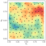
(a) SPs

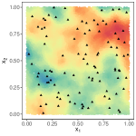
(b) Rands

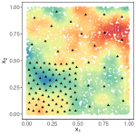
(c) SPs

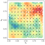
(d) Grids

Figure 1: Rep-points for spatial data with $n=20000$ and multiple location sets. In (a) and (b), the location sets $\{\mathbf{x}_{i}\}_{i=1}^{n}$ follow a uniform distribution on $[0,1]^{2}$. In (c) and (d), $75\%$ of $\{\mathbf{x}_{i}\}_{i=1}^{n}$ follow a uniform distribution on $[0,0.5]^{2}$, and $25\%$ of $\{\mathbf{x}_{i}\}_{i=1}^{n}$ are uniformly distributed over the remaining region.

Finally, we discuss the order of $k$ required for achieving the convergence of $\tilde{f}_{c}$. Mak and Joseph (2018) reported the relationship between the energy distance of SPs and $k$. For a bounded Borel set $\mathcal{X}$ with a nonempty interior, $E(F_{\mathbf{x}},F_{k}^{*})=O\{k^{-1}(\log k)^{-(1-\omega)/(2d)}\}$, where $\omega$ is in $(0,1)$. We consider $E(F_{\mathbf{x}},F_{k}^{*})=O(k^{-1})$ as $k^{-1}$ dominates $(\log k)^{-(1-\omega)/(2d)}$. Then, to satisfy the condition of convergence, i.e., $E(F_{\mathbf{x}},F_{k}^{*})=o_{p}(n^{-2/\gamma})$, we require that $k$ should have a higher order than $O(n^{2/\gamma})$. We can then see that the larger the $\gamma$, the smoother is the process, and the smaller is the order of $k$ needed to ensure the convergence of $\tilde{f}_{c}$.

2.2 Estimated covariance function

Usually, the covariance $c$ is unknown and is replaced by an estimated one, i.e., $\hat{c}$. This section examines the influence of the estimated covariance $\hat{c}$ on the convergence rate of the original process and the conditions on rep-points for the predictive process such that its convergence can achieve the same rate. Similar to the studies by Tuo and Wang (2020) and Wang and Jing (2021), we demonstrate the undersmoothed and oversmoothed cases, where $\hat{\gamma}$ is smaller and larger than $\gamma$, respectively.

Theorem 2.

(Convergence rate of $\tilde{f}_{\hat{c}}$) Assume that the regularity conditions [R1]–[R4] hold for $\hat{c}$ and $\hat{\gamma},\gamma>2$. As $n\to\infty$, $V(\hat{f}_{\hat{c}}-f)=O_{p}\left\{n^{-\{\min(\hat{\gamma},\gamma)-1\}/\hat{\gamma}}\right\}$. Furthermore, assume that $J_{\hat{c}}(f)\preceq O_{p}\{n^{-(\gamma-1-\hat{\gamma})/\hat{\gamma}}\}$ when $\hat{\gamma}>\gamma-1$. Then, for $D_{k}^{*}\subset\{\mathbf{x}_{i}\}_{i=1}^{n}$, if $n^{2/\hat{\gamma}}E(F_{\mathbf{x}},F_{k}^{*})\to 0$ as $k,n\to\infty$, the prediction $\tilde{f}_{\hat{c}}$ achieves a convergence rate identical to that achieved by $\hat{f}_{\hat{c}}$

$$V(\tilde{f}_{\hat{c}}-f)=O_{p}\left\{n^{-\frac{\min(\hat{\gamma},\gamma)-1}{\hat{\gamma}}}\right\}.$$ (6)

Theorem 6 shows the convergence rates of both $\hat{f}_{\hat{c}}$ and $\tilde{f}_{\hat{c}}$. For the undersmoothed case, i.e., $\hat{\gamma}<\gamma$, the convergence rate is $O_{p}\{n^{-(1-1/\hat{\gamma})}\}$. For the oversmoothed case, i.e., $\hat{\gamma}>\gamma$, the convergence rate becomes $O_{p}\{n^{-(\gamma-1)/\hat{\gamma}}\}$. The closer $\hat{\gamma}$ is to $\gamma$, the faster is the convergence. When $\hat{\gamma}=\gamma$, Theorem 6 becomes Theorem 5. Even in the case of an estimated covariance, the convergence rate of $\tilde{f}_{\hat{c}}$ can be identical to that of $\hat{f}_{\hat{c}}$ with sufficient rep-points. To achieve convergence, we require $E(F_{\mathbf{x}},F_{k}^{*})=o_{p}\{n^{-2/\hat{\gamma}}\}$, indicating that $\tilde{f}_{\hat{c}}$ in the undersmoothed case requires additional rep-points than $\tilde{f}_{c}$ to achieve convergence; in the oversmoothed case, $\tilde{f}_{\hat{c}}$ achieves convergence faster.

With an estimated covariance, the following theorem suggests the adjustment of $\tau^{2}$ to improve the convergence rates of $\hat{f}_{\hat{c}}$ and $\tilde{f}_{\hat{c}}$ when $k$ is given and large enough.

Theorem 3.

(Adjusted $\tau^{2}$) Assume that the regularity conditions [R1]–[R4] hold for $\hat{c}$ and $\hat{\gamma},\gamma>2$. If $\tau^{2}=O(n^{-\hat{\gamma}/\gamma+1})$, the prediction based on full data achieves the optimal convergence rate, i.e., $V(\hat{f}_{\hat{c}}-f)=O_{p}\left\{n^{-(1-1/\gamma)}\right\}$ as $n\to\infty$. Furthermore, assume that $J_{\hat{c}}(f)\preceq O_{p}\{n^{(\gamma-1-\hat{\gamma})/\gamma}\}$ when $\hat{\gamma}>\gamma-1$. Then, for $D_{k}^{*}\subset\{\mathbf{x}_{i}\}_{i=1}^{n}$, if $n^{2/\hat{\gamma}}E(F_{\mathbf{x}},F_{k}^{*})\to 0$ as $k,n\to\infty$, the prediction based on the rep-points achieves the optimal convergence rate

$$V(\hat{f}_{\hat{c}}-f)=O_{p}\left\{n^{-(1-1/\gamma)}\right\}.$$

Theorem 3 demonstrates that even with a mis-specified covariance, $\tilde{f}_{\hat{c}}$ and $\hat{f}_{\hat{c}}$ can converge with the same rate as $\tilde{f}_{c}$ and $\hat{f}_{c}$, respectively, by properly adjusting the order of $\tau^{2}$. For the undersmoothed case, the adjusted $\tau^{2}$ has a higher order than $O(1)$, and vice versa. The larger the $|\hat{\gamma}-\gamma|$, the larger is the required adjustment of $\tau^{2}$. For $\hat{\gamma}=\gamma$, we do not require to adjust $\tau^{2}$ and Theorem 3 becomes Theorem 5. Although we can never adjust $\tau^{2}$ to be of the exact order desired, Theorem 3 provides certain guidance. For the example of the undersmoothed case, we can make $\tau^{2}$ larger than the initial value to improve the prediction performance of $\tilde{f}_{\hat{c}}$ and $\hat{f}_{\hat{c}}$.

3 Simulations

This section uses simulated data to show the properties of the complexity parameter $\gamma$, demonstrate the advantages of low-rank approximation with SPs under various scenarios, and confirm our theoretical results. The computations were implemented using R software version 4.1.3 (R Core Team, 2022) with a 72-core Intel(R) Xeon(R) 3.10GHz and 192GB memory processor.

3.1 Complexity parameter $\gamma$

We use the Matérn covariance function as an example to provide an intuitive demonstration of the complexity parameter $\gamma$. Assume that the covariance $c$ is stationary and has the following form:

$$c(\mathbf{x}_{i},\mathbf{x}_{j})=\frac{\sigma^{2}}{\Gamma(\nu)2^{\nu-1}}\left(\frac{\|\mathbf{x}_{i}-\mathbf{x}_{j}\|_{2}}{\psi}\right)^{\nu}\mathcal{K}_{\nu}\left(\frac{\|\mathbf{x}_{i}-\mathbf{x}_{j}\|_{2}}{\psi}\right),$$ (7)

where $\sigma^{2}>0$ is the marginal variance such that $c(\mathbf{x},\mathbf{x})=\sigma^{2}$ for any $\mathbf{x}\in\mathcal{X}$, $\psi>0$ is called the range parameter; $\nu>0$ determines the smoothness of $f(\mathbf{x}_{i})$ (or $Z$) and is termed the smoothness parameter; $\mathcal{K}_{\nu}$ is the modified Bessel function of the second type of order $\nu$.

For obtaining an empirical estimate of $\gamma$, we calculate the eigenvalues of an $n_{0}\times n_{0}$ matrix $\mathbf{C}_{0}=\{c(\mathbf{x}_{i},\mathbf{x}_{j})\}_{i,j=1}^{n_{0}}$, i.e., $\lambda_{01},\ldots,\lambda_{0n_{0}}$, where $\{\mathbf{x}_{i}\}_{i=1}^{n_{0}}$ are uniformly distributed on $[0,1]^{2}$. As $\lambda_{0i}^{-1}=O(i^{\gamma})$, we fit $\{\log i,-\log\lambda_{0i}\}_{i=1}^{n_{0}}$ with a linear regression model and obtain the slope as an estimate of $\gamma$. Fig. 2 shows how $\gamma$ changes with the parameters in the Matérn covariance function, where $\sigma^{2}$ is fixed at $1.5$. In Fig. 2, we set $\psi$ to be $0.063$ and $0.169$ for covering the cases of weak and strong correlations, respectively. Based on other parameters, the complexity parameter $\gamma$ linearly grows with the smoothness parameter $\nu$; this result is in agreement with the discussion reported by Wang and Jing (2021) that $\gamma$ is about $2(\nu+d/2)/d$. In Fig. 2, $\gamma$ increases with $\psi$, though not linearly. Moreover, although $\psi$ varies within a large range, $\gamma$ varies within $0.5$. Compared with $\psi$, $\gamma$ is more sensitive to the value of $\nu$.

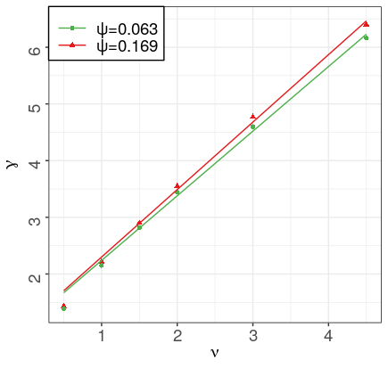
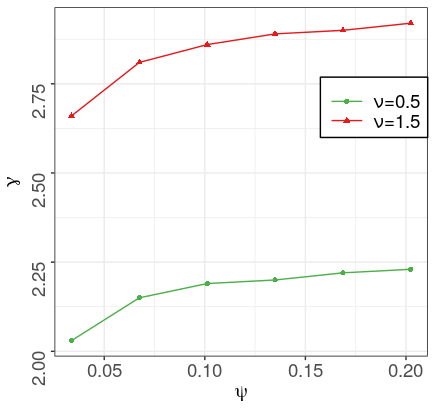
Figure 2: Values of the complex parameter $\gamma$ for the Matérn covariance function (7) under various parameter settings: (a) weak and strong correlations; (b) rough and smooth realizations.

Two Matérn covariance functions with consistent parameters $(\sigma_{1}^{2},\psi_{1},\nu)$ and $(\sigma_{2}^{2},\psi_{2},\nu)$ satisfying $\sigma_{1}^{2}/\psi_{1}^{2\nu}=\sigma_{2}^{2}/\psi_{2}^{2\nu}$ define two equivalent probability measures and thus obtain asymptotically equal predictions (Zhang, 2004). Our simulation and theoretical results taken together demonstrate that the prediction performance is determined by the value of $\gamma$, and two consistent parameter settings should have an asymptotically equal $\gamma$. Table 1 lists the average values of $\gamma$ among $100$ replicates under three consistent parameter settings. The average values get closer as $n_{0}$ increases. This result validates our claim that $\gamma$ is a crucial measure of the complexity of the covariance function.

Table 1: Values of $\gamma$ under consistent parameter settings obtained from the data of increasing size $n_{0}$ of the Matérn covariance function (7).

$(\sigma^{2},\psi,\nu)$	$n_{0}=2000$	$4000$	$6000$	$8000$
$(1.5,0.169,1.5)$	$2.8968$	$2.8982$	$2.9045$	$2.9044$
$(1.0,0.147,1.5)$	$2.8735$	$2.8836$	$2.8936$	$2.8954$
$(2.0,0.186,1.5)$	$2.9114$	$2.9073$	$2.9114$	$2.9099$

3.2 Performance of various rep-points choices

The performance of various rep-points choices under the following four scenarios were tested and compared:

1. Strong correlation: $Z\sim\mathrm{GP}(0,c_{s})$, where $c_{s}$ belongs to the Matérn class in (7) with $\bm{\theta}_{s}=(1.5,0.169,1.5)^{\top}$. The effective range of $Z$ is $0.8$. Here $F_{\mathbf{x}}$ is the uniform distribution on $[0,1]^{2}$, i.e., $U_{[0,1]^{2}}$. Three choices of rep-points (SPs, Grids and Rands) of size $k=(0.10,0.18,0.28,0.40,0.55,0.81,1.12,1.36)\times n^{2/2.9}\approx(36,64,100,144,196,$ $289,400,484)$ were obtained based on the full data. Two mis-specified covariances with $\hat{\bm{\theta}}_{s}=(1.5,0.169,1.0)\top$ and $(1.5,0.169,3.0)^{\top}$ were imposed as the undersmoothed and oversmoothed cases, respectively.

2. Weak correlation: $Z\sim\mathrm{GP}(0,c_{w})$, where $c_{w}$ belongs to the Matérn class in (7) with $\bm{\theta}_{w}=(1.5,0.063,1.5)^{\top}$. The effective range of $Z$ is $0.3$, and $F_{\mathbf{x}}=U_{[0,1]^{2}}$. SPs, Grids and Rands were used to obtain rep-points of sizes $k=(0.66,1.21,1.66,2.05,2.63,3.12,3.64,4.02)\times n^{2/2.8}\approx(289,529,729,900,1156$, $1369,1600,1764)$. Two mis-specified covariances with $\hat{\bm{\theta}}_{w}=(1.5,0.063,1.0)^{\top}$ and $(1.5,0.063,3.0)^{\top}$ were imposed as undersmoothed and oversmoothed cases, respectively.

3. Consistency: The settings are the same as those in the first scenario, although the parameters of the mis-specifed covariances are substituted as $\hat{\bm{\theta}}_{s}=(1.0,0.147,1.5)^{\top}$ and $(2.0,0.186,1.5)^{\top}$ to be consistent with the parameters of $c_{s}$ as discussed in Section 3.1.

4. Nonuniform $F_{\mathbf{x}}$: $Z\sim\mathrm{GP}(0,c_{s})$. The covariance $c_{s}$ is the same as in the first scenario. Here, we have $75\%$ of $\{\mathbf{x}_{i}\}_{i=1}^{n}$ uniformly distributed in $[0.0,0.5]^{2}$ and the other $25\%$ uniformly distributed in the remaining region of $[0,1]^{2}$, as described in Fig. 1(c) and 1(d). Four choices of rep-points were considered, i.e., Grids, Rands and SPs generated by $\{\mathbf{x}_{i}\}_{i=1}^{n}$ (SPs) and by $U_{[0,1]^{2}}$ (SPUs). The size $k$ was the same as that in the first scenario.

For each scenario, we generate $\{(\mathbf{x}_{i},f_{i})\}_{i=1}^{n+n_{t}}$, where $f_{i}=f(\mathbf{x}_{i})$’s are the realizations of the GP $Z$ and $n=n_{t}=5000$. Then, we randomly divide the data into two parts of sizes $n$ and $n_{t}$. Next, we perturb the training data with random noises from $\mathcal{N}(0,0.27)$. Finally, we evaluate $f(\mathbf{x})$ on the remaining $n_{t}$ locations $\{\mathbf{x}_{ti}\}_{i=1}^{n_{t}}$ based on the rep-points or full data. The performance of each method is evaluated in terms of the root mean squared prediction error (RMSPE), i.e., $[n_{t}^{-1}\sum_{i=1}^{n_{t}}\{\tilde{f}_{\hat{c}}(\mathbf{x}_{ti})-f(\mathbf{x}_{ti})\}^{2}]^{1/2}$. We demonstrate the average of RMSPEs over 100 replicates of the abovementioned process in Fig. 3.

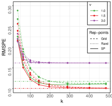
(a) Strong correlation

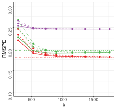
(b) Weak correlation

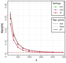
(c) Consistent

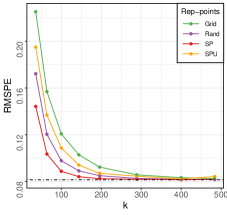
(d) Nonuniform $F_{\mathbf{x}}$

Figure 3: Comparison of various rep-points under four scenarios (a)–(d). The dashed–dotted lines represent the RMSPEs of predictions based on the full data. The legend in (b) is the same as that in (a). CP1, CP2, and TP in (c) correspond to the consistent parameters $\hat{\bm{\theta}}_{s1}$, $\hat{\bm{\theta}}_{s2}$, and true parameter $\bm{\theta}_{s}$, respectively, in the third setting.

In Figs. 3(a) and 3(b), the RMSPEs for $\tilde{f}_{c}$ and $\tilde{f}_{\hat{c}}$ decrease at first and then converge to the levels of $\hat{f}_{c}$ and $\hat{f}_{\hat{c}}$, respectively, as $k$ increases, regardless of the types of rep-points used. This result agrees with our theoretical results that $\tilde{f}_{\hat{c}}$ and $\hat{f}_{\hat{c}}$ may achieve the same convergence rate if $D_{k}^{*}$ (or rep-points) approximate $F_{\mathbf{x}}$ well enough and validates the efficiency of the rep-points. The solid lines representing SPs decline the fastest, whereas the dotted lines have the slowest drop, regardless of whether the imposed/estimated covariance is correct or not. This result indicates that SPs represent the $\{\mathbf{x}_{i}\}_{i=1}^{n}$ better than Grids. Rands exhibit the worst performance because of the lack of the space-filling property.

To understand the influence of the imposed covariance, we compare curves of the same type but shown in different colors. When $k$ is not extremely small, the predictions given by the true covariance have the lowest RMSPEs, indicating that a wrongly specified covariance can typically weaken the prediction performance. When $k$ is quite small, imposing an oversmoothed covariance function may yield a more accurate prediction. A larger value of $\hat{\gamma}$ (or $\hat{\nu}$) results in the earlier convergence of the corresponding method; this result agrees with our theoretical results, according to which the required $k$ for the convergence of $\tilde{f}_{\hat{c}}$ is of order $O(n^{2/\hat{\gamma}})$.

The predictions shown in Fig. 3(a) have smaller RMSPEs than those shown in Fig. 3(b). The second setting involves a more complex structure with a smaller $\psi$ and hence a smaller $\gamma$. Moreover, $\tilde{f}_{\hat{c}}$ and $\tilde{f}_{c}$ in Fig. 3(b) require a larger $k$ to achieve convergence, further demonstrating the influence of shortening of the range parameter $\psi$. In particular, define $K$ as the size of rep-points such that $\tilde{f}_{c}$ based on SPs achieves convergence. Remember that $K$ has a higher order than $O(n^{2/\gamma})$. Then, both $\nu$ and $\psi$ influence $K$. When $\psi$ is fixed, $K$ changes less with $\nu$. For example, $K$ for different lines (in different colors) in Fig. 3(a) are all within $500$. However, when we change the value of $\psi$, $K$ drastically varies. For example, the $K$ for the red solid line in Fig. 3(b) is much larger than that shown in Fig. 3(a).

Figure 3(c) shows the performance of predictions with consistent parameters. Curves represented in different colors but of the same type are approximately coincident. That is, by controlling the choice of rep-points, we can achieve $\tilde{f}_{\hat{c}}$ with consistent $\hat{c}$ to give an asymptotically identical prediction performance. This result is consistent with our discussion reported in Section 3.1 that consistent covariance functions have asymptotic identical values of $\hat{\gamma}$, which determine the performance of $\tilde{f}_{\hat{c}}$. Moreover, we confirmed the conclusion of Zhang (2004), i.e., an incorrect but consistent $\hat{c}$ has the same prediction performance as $c$.

Table 2: $E(F_{k}^{*},F_{n})$ for multiple rep-points with $n=5000$. Furthermore, $k$ is varied in the fourth scenario.

Rep-points	$k=36$	$64$	$100$	$144$	$196$	$289$	$400$	$484$
SPs	$0.001060$	$0.000448$	$0.000233$	$0.000155$	$0.000090$	$0.000177$	$0.000036$	$0.000424$
Rands	$0.014050$	$0.007778$	$0.004843$	$0.003462$	$0.002417$	$0.001805$	$0.001119$	$0.000865$
SPUs	$0.030280$	$0.029645$	$0.029446$	$0.029347$	$0.029260$	$0.029361$	$0.029215$	$0.029606$
Grids	$0.034860$	$0.032329$	$0.031250$	$0.030650$	$0.030270$	$0.029863$	$0.029729$	$0.029670$

Fig. 3(d) shows the performance of $\tilde{f}_{c}$ based on various rep-points when $\{\mathbf{x}_{i}\}_{i=1}^{n}$ are nonuniformly distributed over a compact region $\mathcal{X}$. $\tilde{f}_{c}$ based on SPs and Rands converge earlier than those based on SPUs and Grids. This is because SPs and Rands follow $F_{\mathbf{x}}$, whereas SPUs and Grids follow $U_{[0,1]^{2}}$. In other words, the distribution of rep-points should be as close to $F_{n}$ as possible. SPs meet this requirement by minimizing the energy distance between their empirical distribution and $F_{n}$. For an intuitive comparison, we provide $E(F_{k}^{*},F_{n})$ for the four rep-points in Table 2. All the energy distances decrease as $k$ grows. SPUs and Grids have larger $E(F_{k}^{*},F_{n})$ than SPs and Rands because they follow a distribution different from $F_{\mathbf{x}}$. Even with the same asymptotic distribution, there exist large gaps between the energy distances of SPs and Rands, particularly for small $k$. For example when $k=484$, the $E(F_{n},F_{k}^{*})$ for SPs is $51\%$ smaller than that for Rands. SPs are the most efficient in minimizing $E(F_{k}^{*},F_{n})$.

3.3 Influence of $\hat{c}$

First, we confirm Theorem 6 by exploring the orders of $V(\tilde{f}_{\hat{c}}-f)$ and $V(\tilde{f}_{c}-f)$ with respect to $n$ for a sufficiently large $k$. Let $F_{\mathbf{x}}=U_{[0,1]^{2}}$, $n=1000,1500,\ldots,7000$, and $n_{t}=5000$. For each $n$, we follow the procedure described in Section 3.2 to generate the training data and to predict on the testing location based on SPs and Rands with $k=\lfloor 1.5\times n^{2/2.9}\rfloor$. We consider $c_{w}$ as the true covariance. The values of $\sigma^{2}$ and $\psi$ in $c_{s}$ are fixed; however, $\nu$ is set to be $0.5$ and $1.0$ for undersmoothed covariances and $2.0$ and $3.0$ for oversmoothed ones. Note that we use the covariance in the first scenario such that $\tilde{f}_{\hat{c}}$ and $\tilde{f}_{c}$ converge to $\hat{f}_{\hat{c}}$ and $\hat{f}_{c}$ with a smaller $k$.

The MSPEs for $\tilde{f}_{\hat{c}}$ and $\tilde{f}_{c}$ may well approximate $V(\tilde{f}_{\hat{c}}-f)$ and $V(\tilde{f}_{c}-f)$, respectively, as per the law of large numbers and because $n_{t}$ is quite large. Let MSPE($n$) be the MSPE obtained from the training data of size $n$. Then, by Theorem 6, we have

$$\log\{\mathrm{MSPE}(n)\}\approx-\frac{\min(\gamma,\hat{\gamma})-1}{\hat{\gamma}}\log n+C_{0},$$

where $C_{0}$ is a constant. Our target is to fit the linear regressions above and analyze the slopes.

In Fig. 4, we show the average $\log\{\mathrm{MSPE}(n)\}$s of $100$ replicates (using points) and their fitted lines. For simplicity of discussion, only SPs and Rands are considered. The points for each $n$ and lines in the same color are nearly coincident in most cases, indicating that $\tilde{f}_{\hat{c}}$ and $\tilde{f}_{c}$ have converged to $\hat{f}_{\hat{c}}$ and $\hat{f}_{c}$, respectively. Red lines have the largest negative slopes (NSs) because the prediction under the true covariance has the best performance. For undersmoothed cases, the NSs for SP$(0.5)$ and Rand$(0.5)$ are smaller than those for SP$(1.0)$ and Rand$(1.0)$. For oversmoothed cases, the NSs for SP$(3.0)$ and Rand$(3.0)$ are smaller than those for SP$(2.0)$ and Rand$(2.0)$. The worse the estimate of $\hat{c}$, the larger is the $|\hat{\gamma}-\gamma|$; hence, the worse is the behavior of $\tilde{f}_{\hat{c}}$.

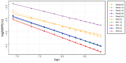
Figure 4: Prediction performance of $\tilde{f}_{\hat{c}}$ and $\tilde{f}_{c}$ with varying $n$ and a sufficiently large $k$. Rand$(0.5)$ in the legend indicates the performance of $\tilde{f}_{\hat{c}}$ with Rands and $\nu=0.5$, and so on for the rest.

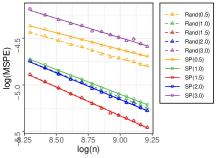
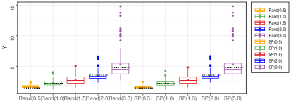
Figure S1: (a) Prediction performance of $\tilde{f}_{\hat{c}}$ and $\tilde{f}_{c}$ with varying $n$ with sufficiently large $k$. (b) Boxplots for $\hat{\gamma}$ and $\gamma$ obtained from the theoretical results. The circles in the middles of the boxes are the average values. The black dotted lines are $\hat{\gamma}$ and $\gamma$ in Section 3.1.

As per (5) and (6), we can evaluate the values of $\hat{\gamma}$ and $\gamma$ through NS. That is, $\hat{\gamma}\approx 1/(1-\mathrm{NS})$ for undersmoothed cases and $\hat{\gamma}\approx(\gamma-1)/(1-\mathrm{NS})$ for oversmoothed cases. The results from $100$ replicates are summarized in Fig. 5. For comparison, we provide the empirical estimates of $\hat{\gamma}$ and $\gamma$ obtained as described in Section 3.1. In most cases, boxes cover the respective black dotted lines well, thereby confirming our theory. For the undersmoothed covariance with $\nu=0.5$, the black dotted lines are considerably lower than their boxes because their complexity parameters are smaller than $2$. Hence our theorems do not apply in these cases. Our theory was further confirmed by setting $\sigma^{2}$ as $0.5$ while maintaining the other parameters fixed for both the true and mis-specified covariances. This verification is illustrated in Fig. S1.

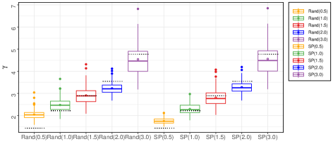
Figure 5: Boxplots for the theoretically obtained $\hat{\gamma}$ and $\gamma$. The circles in the middle of boxes are the average values. The black dotted lines are $\hat{\gamma}$ and $\gamma$, as reported in Section 3.1.

Finally, we demonstrate the improvement of $\tilde{f}_{\hat{c}}$ by adjusting $\tau^{2}$. Still using the first scenario and $\tau^{2}=0.27$, we generate $\{(\mathbf{x}_{i},y_{i})\}_{i=1}^{n}$ with $n=5000$ and $\{(\mathbf{x}_{ti},f_{ti})\}_{i=1}^{n_{t}}$ with $n_{t}=5000$ in the same way. The predictions $\tilde{f}_{c}(\mathbf{x}_{ti})$ and $\tilde{f}_{\hat{c}}(\mathbf{x}_{ti})$ are calculated using the adjusted $\tau^{2}=10^{(-3,2,1,0,0.5,1,1.5,2)}\times 0.27$. Fig. 6 summarizes the average $\log(\rm MSPE)$s over $100$ replicates versus $a_{\tau}=\log_{10}(\tau^{2}/0.27)$. When the correct covariance ($\nu=1.5$) is used, the red curve achieves the lowest MSPE when $a_{\tau}=0$, and this lowest MSPE corresponds to the true value of $\tau^{2}$. When the covariance is mis-specified ($\nu=1$ or $3$), neither of the two curves reach the minimum MSPE under the true $\tau^{2}$. However, the performance of the oversmoothed covariance (with $\nu=3$) improves when $a_{\tau}$ is reduced to $-2$; the performance of the undersmoothed covariance (with $\nu=1$) improves when $a_{\tau}$ is increased to $0.5$. Furthermore, the lowest MSPEs of $\tilde{f}_{\hat{c}}$ are comparable to those of $\tilde{f}_{c}$; this result is in agreement with Theorem 3 that $\tilde{f}_{\hat{c}}$ may have the same convergence rate as $\tilde{f}_{c}$ for an appropriate value of $\tau^{2}$.

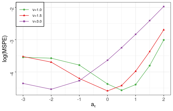
Figure 6: Prediction performance of $\tilde{f}_{\hat{c}}$ and $\tilde{f}_{c}$ with varying $\tau^{2}$.

4 Data Examples

In this section, we explain the advantages of low-rank approximations with an estimated covariance and SPs on two real datasets: annual total precipitation anomalies and total column ozone data. We compare our method with other popular methods such as FRK (Zammit-Mangion and Cressie, 2021), LatticeKrig (Nychka et al., 2016), and autoFRK (Tzeng et al., 2021).

4.1 Annual total precipitation anomalies data

In the first application, we consider the data of annual total precipitation anomalies observed at $7352$ weather stations in the United States in 1962. This dataset was discussed by Kaufman et al. (2008) and Sang and Huang (2012). As shown in Fig. 7, the locations are nonuniformly distributed over an irregular region $\mathcal{X}$. Without an obvious mean trend, nonstationarity or anisotropy (Kaufman et al., 2008), we fit the data with a stationary Gaussian process with mean zero. In particular, we randomly divide the data into training data with $n=7000$ and testing data with $n_{t}=352$. Based on the training data, we apply the Vecchia approximation to obtain an approximated covariance estimation. This approximation can be implemented by the R package GpGp (Guinness et al., 2021), where we set the covariance to be Matérn in (7). Furthermore, we use ExaGeoStat (Abdulah et al., 2018a) to calculate the exact covariance estimation as a benchmark. Using these approximated covariance and SPs of $k=210$, $500$, $750$ and $1000$, we obtain $\tilde{f}_{\hat{c}}(\mathbf{x}_{ti})$s. We calculate the $\mathrm{MSPE}=n_{t}^{-1}\sum_{i=1}^{n_{t}}\{y_{ti}-\tilde{f}_{\hat{c}}(\mathbf{x}_{ti})\}^{2}$ to measure the prediction performance of our method, where $\{y_{ti}\}_{i=1}^{n_{t}}$ are the responses of the testing data.

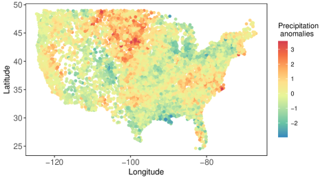
Figure 7: Annual total precipitation anomalies data for $7352$ weather stations in the United States in 1962. The locations are nonuniformly distributed over an irregular region.

Moreover, we consider the method of using the estimated covariance and full data (FULL) and three other popular low-rank approximation methods mentioned earlier, namely, FRK, LatticeKrig, and autoFRK. The FRK performs inference on basic areal units (BAUs). It develops multiresolution basis functions and calculates coefficients by using the expectation-maximization (EM) algorithm. We set two and three levels of resolutions and exponential kernel functions. LatticeKrig induces the basis functions with regular lattices of different levels and uses the Markov random field assumption to develop a sparse precision matrix for random weights. The higher the level, the finer are the grid points. This method can be implemented by the R package LatticeKrig (Nychka et al., 2016). We test the performance of LatticeKrig with smoothness parameters $\nu=0.5$ and $1$, and spatially autoregressive weights AW=$4.1$, $5.0$, and $6.0$, two levels of resolutions, and $15$ grids points at the coarsest resolution. For additional details of these parameters, we refer the readers to Nychka et al. (2015). The autoFRK develops adaptive basis functions corresponding to different scales with thin-plate splines. Based on a maximum number $B$ of basis functions, it selects $B^{*}\leq B$ bases by the Akaike’s information criterion (AIC). The method can be implemented by the R package autoFRK (Tzeng et al., 2021). Here we set $B$ as $210$, $500$, $750$ and $1000$.

We repeat the above process $100$ times and report the average performance of these methods with regard to their MSPEs, computational time (seconds) of covariance estimation and prediction, and the actual number of bases. These results are summarized in Table 3. For FULL and SP$(210)$–$(1000)$, Table 3 only lists the results of predictions using the estimated covariance calculated by GpGp. Based on the exact covariance estimation calculated by the ExaGeoStat, FULL and SP$(210)$–$(1000)$ have MSPEs $0.22096$, $0.31643$, $0.27955$, $0.26083$, and $0.25178$, respectively. For LatticeKrig, we only listed the best result among all the parameter settings, i.e., the result for $\nu=1$ and AW$=6.0$. FRK has the lowest MSPE when the #Bases is small but requires much longer time. Moreover, the decrease in its MSPE is limited when #Bases increases. Furthermore, with multiresolution bases, autoFRK behaves well when #Bases is small. However, its computational time rapidly increases and it cannot be applied when $B$ is larger than about $1000$. LatticeKrig uses more bases and consumes more time. The performance of our method is less superior when #Bases is small because SPs cannot represent the full data locations well. However, the performance is drastically improved as we increase $k$. SP$(1000)$ provides a smaller MSPE with less computational time compared to FRK$(3)$ and LatticeKrig, both of which use more bases. Thus, the superiority of our method is verified.

Table 3: Performance of various methods for the annual total precipitation data. FULL represents the prediction based on full data and estimated covariance obtained by GpGp. SP$(210)$–$(1000)$ represent low-rank approximations based on $210$–$1000$ SPs and estimated covariance obtained by GpGp. FRK$(2)$–$(3)$ represent the FRK method with two and three levels of resolutions, respectively. Furthermore, autoFRK$(210)$–$(1000)$ represent the autoFRK method with $B=210$–$1000$.

Methods	FULL	SP($210$)	SP($500$)	SP($750$)	SP($1000$)	FRK($2$)
MSPE	$0.22077$	$0.31542$	$0.27918$	$0.26183$	$0.25624$	$0.28670$
Time (s)	$213$	$57$	$82$	$101$	$105$	$305$
#Bases	$7000$	$210$	$500$	$750$	$1000$	$210$
Methods	FRK$(3)$	autoFRK($210$)	autoFRK($500$)	autoFRK($750$)	autoFRK($1000$)	LatticeKrig
MSPE	$0.27869$	$0.30461$	$0.26883$	$0.25975$	–	$0.29958$
Time (s)	$4053$	$42$	$113$	$197$	–	$159$
#Bases	$1936$	$205$	$499$	$748$	–	$1258$

4.2 Total column ozone data

In the second application, we demonstrate the feasibility of application of various methods on a large and nonstationary dataset, which includes $173,405$ observations of the level-$2$ total column ozone and their locations. The data were collected and preprocessed by NASA and were discussed by Cressie and Johannesson (2008) and Meng et al. (2020). The region of interest $\mathcal{X}$ has a regular shape. We fit the data with $Z\sim\mathrm{GP}(\mu,c)$, where $\mu$ is a constant and $c(\mathbf{x}_{i},\mathbf{x}_{j})=\sigma^{2}\Gamma(\nu)^{-1}2^{1-\nu}(\|\mathbf{L}\mathbf{x}_{i}-\mathbf{L}\mathbf{x}_{j}\|_{2})^{\nu}\mathcal{K}_{\nu}(\|\mathbf{L}\mathbf{x}_{i}-\mathbf{L}\mathbf{x}_{j}\|_{2})$; here, $\mu$, $\sigma^{2}$, $\nu$, and the $2\times 2$ symmetric matrix $\mathbf{L}$ are the parameters to be evaluated.

We divide the data into two parts: training data with $n=150,000$, and testing data with $n_{t}=23,405$. We evaluate the covariance function using the R package GpGp. The SPs of $k=189$, $500$, $1361$, and $1755$ are generated for facilitating better comparison with the other methods. We fitted the low-rank approximation based on the estimated covariance and SPs induced by the training data and performed predictions on the testing data. For the total column ozone data, only FRK and LatticeKrig are considered for comparison as autoFRK is not applicable because of the large sample size. For implementing FRK, we set two and three levels of resolutions and Matérn kernel functions with $\nu=1.5$. For LatticeKrig, we explore the parameters from the settings described in the previous subsection, and we set $\nu=0.5$, AW$=4.1$, two levels of resolutions, and $15$ grid points at the coarsest resolution. Neither FRK nor LatticeKrig allow smoothly setting the number of bases.

The average results over $100$ runs are summarized in Table 4. Similar to the first example, the MSPE of FRK slightly decreases but its computational cost dramatically increases with an increase in #Bases. LatticeKrig takes the least time. The basis functions induced by the SPs are more efficient. SP$(189)$ is comparable to FRK$(2)$ and consumes much less time. SP$(1361)$ has a lower MSPE than LatticeKrig$(3)$, which uses $3840$ bases. In our method, the main time-consuming process is the generation of the SPs. To address this issue, one can generate SPs from a random subset of the training data without affecting the space-filling property.

Table 4: Performance of various methods for the total column ozone data. LatticeKrig$(2)$ and $(3)$ mean LatticeKrig with two and three levels of resolutions, respectively.

Methods	FRK$(2)$	FRK$(3)$	SP($189$)	SP($500$)
MSPE	$111.33$	$51.17$	$119.97$	$61.38$
Time (s)	$1407$	$11769$	$941$	$1003$
#Bases	$189$	$1755$	$189$	$500$
Methods	SP($1361$)	SP$(1755)$	LatticeKrig$(2)$	LatticeKrig$(3)$
MSPE	$38.02$	$35.51$	$85.09$	$38.55$
Time (s)	$1196$	$1311$	$161$	$278$
#Bases	$1361$	$1755$	$1361$	$3840$

5 Discussion

In this study, we derived the asymptotic performance of a low-rank GP prediction $\tilde{f}_{\hat{c}}$ and investigated the influence of rep-points $D_{k}^{*}$ and estimated covariance $\hat{c}$ on the convergence rate of $\tilde{f}_{\hat{c}}$. Using the concept of energy distance, we demonstrated that the distribution of rep-points should be as close as possible to that of the full data locations. It motivates the utilization of SPs, which have space-fillingness but also can best mimic the full data. We set the order of $k$ such that the convergence rate of $\tilde{f}_{\hat{c}}$ is equal to that of $\hat{f}_{\hat{c}}$ under certain regularity conditions. With $\hat{\gamma}$ indicating the complexity of $\hat{c}$, we provided the convergence rates of $\tilde{f}_{\hat{c}}$ and $\hat{f}_{\hat{c}}$ when sufficient rep-points are given, i.e., $V(\tilde{f}_{\hat{c}}-f)=V(\hat{f}_{\hat{c}}-f)=O_{p}[n^{-\{\min(\hat{\gamma},\gamma)-1\}/\hat{\gamma}}]$. This indicates that the closer the $\hat{\gamma}$ is to $\gamma$, the faster is the convergence. Moreover, we demonstrated the performance improvement of $\tilde{f}_{\hat{c}}$ by adjusting the order of the nugget effect. We demonstrated the value of $\gamma$ and confirmed our theoretical results via extensive numerical studies. Using two examples of real data, we validated the prediction of $\tilde{f}_{\hat{c}}$ based on SPs by comparing our results with the results obtained using other existing low-rank approximation methods.

In some of the existing methods, such as FRK and LatticeKrig, multiresolution bases are desirable to capture information at different scales. In this way, they can better represent the local dependency and evaluate the covariance. In this study, we used the bases induced by SPs without multiresolution capability because we fixed the covariance and focused only on the prediction accuracy. We preferred to consider the tasks of covariance estimation and prediction separately because they require different configurations of rep-points. Literature in the field of spatial designs suggests future avenues, e.g., samples in clusters behave better for covariance estimation, whereas widely distributed samples are better for prediction (Zhu and Stein, 2005, 2006; Barbian and Assunção, 2017). Therefore, one possible extension of our work is the configuration of rep-points for covariance estimation.

Appendix A Appendix: Proofs of Theorems

First, we introduce certain necessary notations. For two positive sequences $a_{n}$ and $b_{n}$, $a_{n}\asymp b_{n}$ indicates that there are two positive constants $A$ and $B$ such that $A\leq a_{n}/b_{n}\leq B$. Furthermore, $a_{n}\preceq b_{n}$ indicates there is a $B>0$ such that $a_{n}\leq Bb_{n}$; $a_{n}\succeq b_{n}$ indicates there is an $A>0$ such that $a_{n}\geq Ab_{n}$.

A.1 Proofs of Theorems 5 and 6

Proof.

Using the triangle inequality, we have

$$V(\tilde{f}_{\hat{c}}-f)\leq V(\tilde{f}_{\hat{c}}-\hat{f}_{\hat{c}})+V(\hat{f}_{\hat{c}}-f),$$

where the first term shows the influence of rep-points and the second term shows the influence of the estimated covariance $\hat{c}$. In the following proofs, we bound the two terms.

Step 1: order of $V(\hat{f}_{\hat{c}}-f)$.

We discuss the order of $V(\hat{f}_{\hat{c}}-f)$ in two cases: $\hat{\gamma}<\gamma_{f}$ and $\hat{\gamma}>\gamma_{f}$.

For the case of $2<\hat{\gamma}<\gamma_{f}$, because $J_{c_{f}}(f)<\infty$, we have

$$J_{\hat{c}}(f)=\sum_{r=1}^{\infty}\hat{\rho}_{r}\hat{f}_{r}^{2}\asymp\sum_{r=1}^{\infty}r^{\hat{\gamma}}\hat{f}_{r}^{2}\preceq\sum_{r=1}^{\infty}r^{\gamma_{f}}\hat{f}_{r}^{2}\asymp\sum_{r=1}^{\infty}\rho_{r,f}f_{r,f}^{2}=J_{c_{f}}(f)<\infty.$$

Then, using Lemma 3 in the Supplementary Material, as $\tau^{2}/(2n)\to 0$ and $n\{\tau^{2}/(2n)\}^{2/\hat{\gamma}}\to\infty$,

$$\left(V+\frac{\tau^{2}}{2n}J_{\hat{c}}\right)(\hat{f}_{\hat{c}}-f)=O_{p}\left\{n^{-1}\left(\frac{\tau^{2}}{2n}\right)^{-1/\hat{\gamma}}+\frac{\tau^{2}}{2n}\right\}.$$ (8)

Using $\tau^{2}\asymp O(1)$, $V(\hat{f}_{\hat{c}}-f)\preceq\left(V+\frac{\tau^{2}}{2n}J_{\hat{c}}\right)(\hat{f}_{\hat{c}}-f)=O_{p}\{n^{-(1-1/\hat{\gamma})}\}$.

For the case of $\hat{\gamma}>\gamma_{f}$, when $\tau^{2}\asymp O(1)$, from Lemma 6,

$$V(\hat{f}_{\hat{c}}-f)\preceq O_{p}\left\{n^{-\gamma_{f}/\hat{\gamma}}+n^{-(1-1/\hat{\gamma})}\right\}.$$

Then, $V(\hat{f}_{\hat{c}}-f)\preceq O_{p}\left\{n^{-(1-1/\hat{\gamma})}\right\}$ if $\gamma_{f}<\hat{\gamma}\leq\gamma_{f}+1$; $V(\hat{f}_{\hat{c}}-f)\preceq O_{p}\left\{n^{-\gamma_{f}/\hat{\gamma}}\right\}$ if $\hat{\gamma}>\gamma_{f}+1$.

Combining the abovementioned results, we have

$$V(\hat{f}_{\hat{c}}-f)\preceq O_{p}\left\{n^{-(1-1/\hat{\gamma})}\right\}\quad\text{if}\quad\hat{\gamma}\leq\gamma_{f}+1,$$

$$V(\hat{f}_{\hat{c}}-f)\preceq O_{p}\left\{n^{-\gamma_{f}/\hat{\gamma}}\right\}\quad\text{if}\quad\hat{\gamma}>\gamma_{f}+1.$$

Now, we discuss the relationship of $\gamma_{f}$ with $\gamma$. Although $f$ is the realization of $Z$, $\gamma_{f}$ is lower than $\gamma$ with probability $1$ (Driscoll, 1973; Kanagawa et al., 2018; Steinwart, 2019). Assume that there exists $m>d/2$ such that for any $w\in\mathbb{R}^{d}$,

$$c_{1}(1+\|\bm{w}\|_{2}^{2})^{-m}\leq\mathcal{F}_{c}(\bm{w})\leq c_{2}(1+\|\bm{w}\|_{2}^{2})^{-m},$$

where $\mathcal{F}_{c}(\bm{w})=(2\pi)^{-d/2}\int_{\mathbb{R}^{d}}c(\mathbf{x})e^{-i\mathbf{x}^{\top}\bm{w}}\bm{\mathrm{d}}\mathbf{x}$. Then, $m$ indicates the smoothness of $c$. From Lemma F.2 of Wang and Jing (2021), $\rho_{r}^{-1}\asymp r^{-2m/d}$ with a strictly positive probability. That is, $r^{\gamma}\asymp r^{2m/d}$. If we use $m_{f}$ to indicate the smoothness of $f$, as per the work of Kanagawa et al. (2018), $m_{f}$ is about $m-d/2$. This expression indicates that

$$r^{2m_{f}/d}\asymp r^{2(m-d/2)/d}\asymp r^{2m/d-1}\asymp r^{\gamma-1}.$$

Then, $\gamma_{f}$ is around $\gamma-1$, and

$$V(\hat{f}_{\hat{c}}-f)\preceq O_{p}\left\{n^{-(1-1/\hat{\gamma})}\right\}\quad\text{if}\quad\hat{\gamma}\leq\gamma,$$

$$V(\hat{f}_{\hat{c}}-f)\preceq O_{p}\left\{n^{-(\gamma-1)/\hat{\gamma}}\right\}\quad\text{if}\quad\hat{\gamma}>\gamma.$$

Step 2: order of $V(\tilde{f}_{\hat{c}}-\hat{f}_{\hat{c}})$.

This step follows the proof of Theorem 3 in Ma et al. (2015). Let $\tilde{f}_{p}$ be the projection of $\hat{f}_{\hat{c}}$ on $\mathcal{H}_{k,\hat{c}}^{*}=\mathrm{span}\{\hat{c}(\cdot,\mathbf{x}_{i}^{*})\}_{i=1}^{k}$. Then,

$$\tilde{f}_{\hat{c}}-\hat{f}_{\hat{c}}=(\tilde{f}_{\hat{c}}-\tilde{f}_{p})+(\tilde{f}_{p}-\hat{f}_{\hat{c}}).$$ (9)

We first discuss the order of $V(\tilde{f}_{p}-\hat{f}_{\hat{c}})$. As $\hat{f}_{\hat{c}}\in\mathcal{H}_{\hat{c}}$, $J_{\hat{c}}(\tilde{f}_{p},\hat{f}_{\hat{c}}-\tilde{f}_{p})=0$. For any $\eta$ and $\xi$ in $\mathcal{H}_{\hat{c}}$, let

$$A_{\eta,\xi}(\alpha)=\frac{1}{n}\sum_{i=1}^{n}\{y_{i}-(\eta+\alpha\xi)(\mathbf{x}_{i})\}^{2}+\frac{\tau^{2}}{2n}J_{\hat{c}}(\eta+\alpha\xi).$$

Hence,

$$\frac{\partial A_{\eta,\xi}(\alpha)}{\partial\alpha}|_{\alpha=0}=-\frac{2}{n}\sum_{i=1}^{n}\{y_{i}-\eta(\mathbf{x}_{i})\}\xi(\mathbf{x}_{i})+2\frac{\tau^{2}}{2n}J_{\hat{c}}(\eta,\xi).$$

As $\hat{f}_{\hat{c}}$ is the minimizer over $\mathcal{H}_{\hat{c}}$, $A_{\eta,\xi}(\alpha=0)$ achieves the minimum at $\eta=\hat{f}_{\hat{c}}$ and $\xi=\hat{f}_{\hat{c}}-\tilde{f}_{p}$. Then,

$$\frac{\tau^{2}}{2n}J_{\hat{c}}(\hat{f}_{\hat{c}},\hat{f}_{\hat{c}}-\tilde{f}_{p})=\frac{1}{n}\sum_{i=1}^{n}\{y_{i}-\hat{f}_{\hat{c}}(\mathbf{x}_{i})\}\{\hat{f}_{\hat{c}}(\mathbf{x}_{i})-\tilde{f}_{p}(\mathbf{x}_{i})\}.$$

With the fact that $J_{\hat{c}}(\tilde{f}_{p},\hat{f}_{\hat{c}}-\tilde{f}_{p})=0$, we have

$$\frac{\tau^{2}}{2n}J_{\hat{c}}(\hat{f}_{\hat{c}}-\tilde{f}_{p}) =\frac{1}{n}\sum_{i=1}^{n}\{y_{i}-\hat{f}_{\hat{c}}(\mathbf{x}_{i})\}\{\hat{f}_{\hat{c}}(\mathbf{x}_{i})-\tilde{f}_{p}(\mathbf{x}_{i})\}$$

$$=\frac{1}{n}\sum_{i=1}^{n}\{y_{i}-f(\mathbf{x}_{i})\}\{\hat{f}_{\hat{c}}(\mathbf{x}_{i})-\tilde{f}_{p}(\mathbf{x}_{i})\}+\frac{1}{n}\sum_{i=1}^{n}\{f(\mathbf{x}_{i})-\hat{f}_{\hat{c}}(\mathbf{x}_{i})\}\{\hat{f}_{\hat{c}}(\mathbf{x}_{i})-\tilde{f}_{p}(\mathbf{x}_{i})\}$$

$$=S_{1}+S_{2}.$$

For $S_{1}$, we write the term $\hat{f}_{\hat{c}}-\tilde{f}_{p}$ as $\hat{f}_{\hat{c}}-\tilde{f}_{p}=\sum_{r=1}^{\infty}(\hat{f}_{\hat{c}}-\tilde{f}_{p})_{r}\hat{\phi}_{r}$, where $(\hat{f}_{\hat{c}}-\tilde{f}_{p})_{r}=V(\hat{f}_{\hat{c}}-\tilde{f}_{p},\hat{\phi}_{r})$ and $\hat{\phi}_{r}$s are the eigenfunctions of $\hat{c}$. Then,

$$S_{1}=\sum_{r=1}^{\infty}(\hat{f}_{\hat{c}}-\tilde{f}_{p})_{r}\left[\frac{1}{n}\sum_{i=1}^{n}\{y_{i}-f(\mathbf{x}_{i})\}\hat{\phi}_{r}(\mathbf{x}_{i})\right].$$

Using the Cauchy–Schwartz inequality,

$$S_{1}^{2} \leq\left\{\sum_{r=1}^{\infty}(\hat{f}_{\hat{c}}-\tilde{f}_{p})_{r}^{2}\left(1+\frac{\tau^{2}}{2n}\hat{\rho}_{r}\right)\right\}\cdot\sum_{r=1}^{\infty}\frac{1}{1+\hat{\rho}_{r}\tau^{2}/(2n)}\left[\frac{1}{n}\sum_{i=1}^{n}\{y_{i}-f(\mathbf{x}_{i})\}\hat{\phi}_{r}(\mathbf{x}_{i})\right]^{2}$$

$$=\left(V+\frac{\tau^{2}}{2n}J_{\hat{c}}\right)(\hat{f}_{\hat{c}}-\tilde{f}_{p})\cdot\sum_{r=1}^{\infty}\frac{1}{1+\hat{\rho}_{r}\tau^{2}/(2n)}\hat{Z}_{r}^{2},$$

where $\hat{Z}_{r}=n^{-1}\sum_{i=1}^{n}\{y_{i}-f(\mathbf{x}_{i})\}\hat{\phi}_{r}(\mathbf{x}_{i})$. Because $\mathbb{E}(\hat{Z}_{r}^{2})=\mathbb{E}[n^{-2}\sum_{i=1}^{n}\{y_{i}-f(\mathbf{x}_{i})\}^{2}\hat{\phi}_{r}(\mathbf{x}_{i})^{2}]=n^{-1}\mathbb{E}\{y_{i}-f(\mathbf{x}_{i})\}^{2}=O(n^{-1})$, we have

$$\sum_{r=1}^{\infty}\frac{1}{1+\hat{\rho}_{r}\tau^{2}/(2n)}\hat{Z}_{r}^{2}=\sum_{r=1}^{\infty}\frac{1}{1+\hat{\rho}_{r}\tau^{2}/(2n)}O_{p}(n^{-1})=O_{p}\left\{n^{-1}\left(\frac{\tau^{2}}{2n}\right)^{-1/\hat{\gamma}}\right\},$$

where the second equality is obtained from Lemma 1. Therefore,

$$S_{1}\leq\left\{\left(V+\frac{\tau^{2}}{2n}J_{\hat{c}}\right)(\hat{f}_{\hat{c}}-\tilde{f}_{p})\right\}^{1/2}O_{p}\left\{n^{-1/2}\left(\frac{\tau^{2}}{2n}\right)^{-1/(2\hat{\gamma})}\right\}.$$

Now, we examine the order of $S_{2}$. From Lemma 2, when $n\{\tau^{2}/(2n)\}^{2/\hat{\gamma}}\to\infty$, let $\eta=f-\hat{f}_{\hat{c}}$ and $\xi=\hat{f}_{\hat{c}}-\tilde{f}_{p}$,

$$S_{2} =V(f-\hat{f}_{\hat{c}},\hat{f}_{\hat{c}}-\tilde{f}_{p})+\left\{\left(V+\frac{\tau^{2}}{2n}J_{\hat{c}}\right)(f-\hat{f}_{\hat{c}})\left(V+\frac{\tau^{2}}{2n}J_{\hat{c}}\right)(\hat{f}_{\hat{c}}-\tilde{f}_{p})\right\}^{1/2}o_{p}(1)$$

$$\leq\{V(f-\hat{f}_{\hat{c}})V(\hat{f}_{\hat{c}}-\tilde{f}_{p})\}^{1/2}+\left\{\left(V+\frac{\tau^{2}}{2n}J_{\hat{c}}\right)(f-\hat{f}_{\hat{c}})\left(V+\frac{\tau^{2}}{2n}J_{\hat{c}}\right)(\hat{f}_{\hat{c}}-\tilde{f}_{p})\right\}^{1/2}o_{p}(1)$$

$$\leq\left\{\left(V+\frac{\tau^{2}}{2n}J_{\hat{c}}\right)(f-\hat{f}_{\hat{c}})\left(V+\frac{\tau^{2}}{2n}J_{\hat{c}}\right)(\hat{f}_{\hat{c}}-\tilde{f}_{p})\right\}^{1/2}\{1+o_{p}(1)\}.$$

By Lemma 4, for $\hat{f}_{\hat{c}}-\tilde{f}_{p}\in\mathcal{H}_{\hat{c}}\ominus\mathcal{H}_{k,\hat{c}}^{*}$, we have $V(\hat{f}_{\hat{c}}-\tilde{f}_{p})=o_{p}\{J_{\hat{c}}(\hat{f}_{\hat{c}}-\tilde{f}_{p})\tau^{2}/(2n)\}$. Then,

$$\left(V+\frac{\tau^{2}}{2n}J_{\hat{c}}\right)(\hat{f}_{\hat{c}}-\tilde{f}_{p}) \asymp\frac{\tau^{2}}{2n}J_{\hat{c}}(\hat{f}_{\hat{c}}-\tilde{f}_{p})$$

$$=S_{1}+S_{2}$$

$$\leq\left\{\left(V+\frac{\tau^{2}}{2n}J_{\hat{c}}\right)(\hat{f}_{\hat{c}}-\tilde{f}_{p})\right\}^{1/2}O_{p}\left\{n^{-1/2}\left(\frac{\tau^{2}}{2n}\right)^{-1/(2\hat{\gamma})}\right\}$$

$$\quad+\left\{\left(V+\frac{\tau^{2}}{2n}J_{\hat{c}}\right)(f-\hat{f}_{\hat{c}})\left(V+\frac{\tau^{2}}{2n}J_{\hat{c}}\right)(\hat{f}_{\hat{c}}-\tilde{f}_{p})\right\}^{1/2}\{1+o_{p}(1)\}.$$

By solving the above inequality, we get

$$\left(V+\frac{\tau^{2}}{2n}J_{\hat{c}}\right)(\hat{f}_{\hat{c}}-\tilde{f}_{p}) \preceq O_{p}\left\{n^{-1}\left(\frac{\tau^{2}}{2n}\right)^{-1/\hat{\gamma}}\right\}+\left(V+\frac{\tau^{2}}{2n}J_{\hat{c}}\right)(f-\hat{f}_{\hat{c}}).$$ (10)

Now, we examine the order of $V(\tilde{f}_{\hat{c}}-\tilde{f}_{p})$. Because $\hat{f}_{\hat{c}}$ is the minimizer of $n^{-1}\sum_{i=1}^{n}\{y_{i}-\eta(\mathbf{x}_{i})\}^{2}+\tau^{2}/(2n)J_{\hat{c}}(\eta)$ over $\mathcal{H}_{\hat{c}}$, $A_{\eta,\xi}(\alpha=0)$ achieves the minimum with $\eta=\hat{f}_{\hat{c}}$ and $\xi=\tilde{f}_{\hat{c}}-\tilde{f}_{p}$. Then, we have

$$\frac{\tau^{2}}{2n}J_{\hat{c}}(\hat{f}_{\hat{c}},\tilde{f}_{\hat{c}}-\tilde{f}_{p})=\frac{1}{n}\sum_{i=1}^{n}\{y_{i}-\hat{f}_{\hat{c}}(\mathbf{x}_{i})\}\{\tilde{f}_{\hat{c}}(\mathbf{x}_{i})-\tilde{f}_{p}(\mathbf{x}_{i})\}.$$ (11)

Because $\tilde{f}_{\hat{c}}$ is the minimizer of $n^{-1}\sum_{i=1}^{n}\{y_{i}-\eta(\mathbf{x}_{i})\}^{2}+\tau^{2}/(2n)J_{\hat{c}}(\eta)$ over $\mathcal{H}_{k,\hat{c}}^{*}\subset\mathcal{H}_{\hat{c}}$, $A_{\eta,\xi}(\alpha=0)$ achieves the minimum with $\eta=\tilde{f}_{\hat{c}}$ and $\xi=\tilde{f}_{\hat{c}}-\tilde{f}_{p}$. Then, we have

$$\frac{\tau^{2}}{2n}J_{\hat{c}}(\tilde{f}_{\hat{c}},\tilde{f}_{\hat{c}}-\tilde{f}_{p})=\frac{1}{n}\sum_{i=1}^{n}\{y_{i}-\tilde{f}_{\hat{c}}(\mathbf{x}_{i})\}\{\tilde{f}_{\hat{c}}(\mathbf{x}_{i})-\tilde{f}_{p}(\mathbf{x}_{i})\}$$ (12)

By combining (11) with (12), we obtain

$$\frac{\tau^{2}}{2n}J_{\hat{c}}(\tilde{f}_{\hat{c}}-\hat{f}_{\hat{c}},\tilde{f}_{\hat{c}}-\tilde{f}_{p})=\frac{1}{n}\sum_{i=1}^{n}\{\hat{f}_{\hat{c}}(\mathbf{x}_{i})-\tilde{f}_{\hat{c}}(\mathbf{x}_{i})\}\{\tilde{f}_{\hat{c}}(\mathbf{x}_{i})-\tilde{f}_{p}(\mathbf{x}_{i})\}.$$

Because $\tilde{f}_{p}$ is the projection of $\hat{f}_{\hat{c}}$ on $\mathcal{H}_{k,\hat{c}}^{*}$ and $\tilde{f}_{\hat{c}}-\tilde{f}_{p}\in\mathcal{H}_{k,\hat{c}}^{*}$, we have $J_{\hat{c}}(\hat{f}_{\hat{c}}-\tilde{f}_{p},\tilde{f}_{\hat{c}}-\tilde{f}_{p})=0$. Therefore,

$$\frac{\tau^{2}}{2n}J_{\hat{c}}(\tilde{f}_{\hat{c}}-\tilde{f}_{p})=\frac{1}{n}\sum_{i=1}^{n}\{\hat{f}_{\hat{c}}(\mathbf{x}_{i})-\tilde{f}_{\hat{c}}(\mathbf{x}_{i})\}\{\tilde{f}_{\hat{c}}(\mathbf{x}_{i})-\tilde{f}_{p}(\mathbf{x}_{i})\},$$

and

$$\frac{1}{n}\sum_{i=1}^{n}\{\tilde{f}_{\hat{c}}(\mathbf{x}_{i})-\tilde{f}_{p}(\mathbf{x}_{i})\}^{2}+\frac{\tau^{2}}{2n}J_{\hat{c}}(\tilde{f}_{\hat{c}}-\tilde{f}_{p})=\frac{1}{n}\sum_{i=1}^{n}\{\hat{f}_{\hat{c}}(\mathbf{x}_{i})-\tilde{f}_{p}(\mathbf{x}_{i})\}\{\tilde{f}_{\hat{c}}(\mathbf{x}_{i})-\tilde{f}_{p}(\mathbf{x}_{i})\}.$$ (13)

By Lemma 2, the left hand side in (13) equals

$$V(\tilde{f}_{\hat{c}}-\tilde{f}_{p})+o_{p}\left\{\left(V+\frac{\tau^{2}}{2n}J_{\hat{c}}\right)(\tilde{f}_{\hat{c}}-\tilde{f}_{p})\right\}+\frac{\tau^{2}}{2n}J_{\hat{c}}(\tilde{f}_{\hat{c}}-\tilde{f}_{p})=\left(V+\frac{\tau^{2}}{2n}J_{\hat{c}}\right)(\tilde{f}_{\hat{c}}-\tilde{f}_{p})\{1+o_{p}(1)\},$$ (14)

and the right hand side in (13) equals

$$V(\hat{f}_{\hat{c}}-\tilde{f}_{p},\tilde{f}_{\hat{c}}-\tilde{f}_{p})+o_{p}\left\{\left(V+\frac{\tau^{2}}{2n}J_{\hat{c}}\right)(\tilde{f}_{\hat{c}}-\tilde{f}_{p})\left(V+\frac{\tau^{2}}{2n}J_{\hat{c}}\right)(\hat{f}_{\hat{c}}-\tilde{f}_{p})\right\}^{1/2}$$ (15)

$$\leq \left\{\left(V+\frac{\tau^{2}}{2n}J_{\hat{c}}\right)(\tilde{f}_{\hat{c}}-\tilde{f}_{p})\left(V+\frac{\tau^{2}}{2n}J_{\hat{c}}\right)(\hat{f}_{\hat{c}}-\tilde{f}_{p})\right\}^{1/2}\{1+o_{p}(1)\}.$$

Combining (14) and (15), we have

$$\left(V+\frac{\tau^{2}}{2n}J_{\hat{c}}\right)(\tilde{f}_{\hat{c}}-\tilde{f}_{p})\{1+o_{p}(1)\}\preceq\left\{\left(V+\frac{\tau^{2}}{2n}J_{\hat{c}}\right)(\tilde{f}_{\hat{c}}-\tilde{f}_{p})\left(V+\frac{\tau^{2}}{2n}J_{\hat{c}}\right)(\hat{f}_{\hat{c}}-\tilde{f}_{p})\right\}^{1/2}\{1+o_{p}(1)\}.$$

Therefore,

$$\left(V+\frac{\tau^{2}}{2n}J_{\hat{c}}\right)(\tilde{f}_{\hat{c}}-\tilde{f}_{p})\leq\left(V+\frac{\tau^{2}}{2n}J_{\hat{c}}\right)(\hat{f}_{\hat{c}}-\tilde{f}_{p}).$$ (16)

With (9), (10) and (16), we obtain the order of the first term

$$\left(V+\frac{\tau^{2}}{2n}J_{\hat{c}}\right)(\tilde{f}_{\hat{c}}-\hat{f}_{\hat{c}})\preceq O_{p}\left\{n^{-1}\left(\frac{\tau^{2}}{2n}\right)^{-1/\hat{\gamma}}\right\}+\left(V+\frac{\tau^{2}}{2n}J_{\hat{c}}\right)(\hat{f}_{\hat{c}}-f).$$ (17)

For $2<\hat{\gamma}<\gamma_{f}$, from (8) and $\tau^{2}\asymp O(1)$, we have

$$V(\tilde{f}_{\hat{c}}-\hat{f}_{\hat{c}})\preceq O_{p}\{n^{-(1-1/\hat{\gamma})}\}.$$

For $\hat{\gamma}>\gamma_{f}$, from Lemma 6, condition $J_{\hat{c}}(f)\preceq O_{p}\{n^{-\{\gamma-1-\hat{\gamma}\}/\hat{\gamma}}\}$ and $\tau^{2}\asymp O(1)$, we have

$$\left(V+\frac{\tau^{2}}{2n}J_{\hat{c}}\right)(\tilde{f}_{\hat{c}}-\hat{f}_{\hat{c}}) \preceq V(\tilde{f}_{\hat{c}}-\hat{f}_{\hat{c}})+\frac{\tau^{2}}{2n}J_{\hat{c}}(\hat{f}_{\hat{c}})+\frac{\tau^{2}}{2n}J_{\hat{c}}(f)$$

$$\preceq O_{p}\{n^{-\gamma_{f}/\hat{\gamma}}+n^{-(1-1/\hat{\gamma})}\}.$$

On substituting the above into (17), we obtain (6). ∎

A.2 Proof of Theorem 3

Proof.

The proof of Theorem 3 follows that of Theorem 6 but takes $\tau^{2}=O(n^{-\hat{\gamma}/\gamma+1})$. ∎

Supplementary Material: Large-Scale Low-Rank Gaussian Process Prediction with Support Points

S1. Lemmas

Herein, we provide the lemmas that will be used in the proofs of the theorems. Remember that $\mathcal{H}_{c}=\{\eta:J_{c}(\eta)=\sum_{r=1}^{\infty}\rho_{r}\eta_{r}^{2}<\infty\}$ is the reproducing kernel Hilbert space (RKHS) induced by the covariance $c$, $\mathcal{H}_{n,c}=\mathrm{span}\{c(\mathbf{x}_{i},\cdot)\}_{i=1}^{n}$ and $\mathcal{H}_{k,c}^{*}=\mathrm{span}\{c(\mathbf{x}_{i}^{*},\cdot)\}_{i=1}^{k}$, where $\mathbf{x}_{i}^{*}$’s are the rep-points. Let us denote the complexity of $f$ as $\gamma_{f}=\max\{\zeta:f\in\mathcal{H}_{c_{\eta}}\text{ where }c_{\eta}\text{ has complexity }\zeta\}$. There exists a kernel function $c_{f}$ with complexity $\gamma_{f}$ such that $f\in\mathcal{H}_{c_{f}}$.

Lemma 1.

Under the regularity condition [R3], we have

$$\sum_{r=1}^{\infty}\left\{1+\rho_{r}\frac{\tau^{2}}{2n}\right\}^{-1}=O\left\{\left(\frac{\tau^{2}}{2n}\right)^{-1/\gamma}\right\}.$$

Proof.

The proof of Lemma 1 follows that of Lemma 9.1 in Gu (2013):

$$\sum_{r=1}^{\infty}\left\{1+\rho_{r}\frac{\tau^{2}}{2n}\right\}^{-1} =\sum_{r\geq\{\tau^{2}/(2n)\}^{-1/\gamma}}\left\{1+\rho_{r}\frac{\tau^{2}}{2n}\right\}^{-1}+\sum_{r<\{\tau^{2}/(2n)\}^{-1/\gamma}}\left\{1+\rho_{r}\frac{\tau^{2}}{2n}\right\}^{-1}$$

$$=O\left\{\int_{\{\tau^{2}/(2n)\}^{-1/\gamma}}^{\infty}\frac{1}{1+r^{\gamma}\tau^{2}/(2n)}\mathrm{d}r\right\}+O(1)$$

$$=O\left\{\int_{1}^{\infty}\left(\frac{\tau^{2}}{2n}\right)^{-1/\gamma}\gamma^{-1}\frac{1}{1+z}z^{1/\gamma-1}\mathrm{d}z\right\}+O(1)$$

$$=O\left\{\left(\frac{\tau^{2}}{2n}\right)^{-1/\gamma}\right\}+O(1)$$

$$=O\left\{\left(\frac{\tau^{2}}{2n}\right)^{-1/\gamma}\right\}.$$

∎

Lemma 2.

Under the regularity conditions [R1]–[R4], when $\tau^{2}/(2n)\to 0$ and $n\{\tau^{2}/(2n)\}^{2/\gamma}\to\infty$, we have

$$\frac{1}{n}\sum_{i=1}^{n}\eta(\mathbf{x}_{i})\xi(\mathbf{x}_{i})=V(\eta,\xi)+\left\{\left(V+\frac{\tau^{2}}{2n}J_{c}\right)(\eta)\left(V+\frac{\tau^{2}}{2n}J_{c}\right)(\xi)\right\}^{1/2}o_{p}(1)$$

for all $\eta$ and $\xi$ in $\mathcal{H}_{c}$.

Proof.

This is Lemma S3 in Ma et al. (2015). ∎

Lemma 3.

Assume that the regularity conditions [R1]–[R4] hold, and that $J_{\hat{c}}(f)<\infty$. Then, as $\tau^{2}/(2n)\to 0$ and $n\{\tau^{2}/(2n)\}^{2/\hat{\gamma}}\to\infty$, we have

$$\left(V+\frac{\tau^{2}}{2n}J_{\hat{c}}\right)(\hat{f}_{\hat{c}}-f)=O_{p}\left\{n^{-1}\left(\frac{\tau^{2}}{2n}\right)^{-1/\hat{\gamma}}+\frac{\tau^{2}}{2n}\right\}.$$

Proof.

This lemma can be derived from Theorem 2 of Ma et al. (2015) or Theorem 9.17 of Gu (2013). ∎

Lemma 4.

Under the regularity conditions [R1]–[R4], if $\{\tau^{2}/(2n)\}^{-1/\gamma}E(F_{\mathbf{x}},F_{k}^{*})^{1/2}\to 0$, for any $\eta\in\mathcal{H}_{c}\ominus\mathcal{H}_{k,c}^{*}$, then we have

$$V(\eta)=o_{p}\left\{\frac{\tau^{2}}{2n}J_{c}(\eta)\right\}.$$

Proof.

For any $\eta\in\mathcal{H}_{c}\ominus\mathcal{H}_{k,c}^{*}$, we have $\eta(\mathbf{x}_{i}^{*})=\langle\eta(\cdot),c(\mathbf{x}_{i}^{*},\cdot)\rangle_{\mathcal{H}_{c}}=0$. The first equality corresponds to $\eta\in\mathcal{H}_{c}$ and the second one to $\eta\notin\mathcal{H}_{k,c}^{*}$. Thus, $\sum_{i=1}^{k}\eta^{2}(\mathbf{x}_{i}^{*})=0$. Remember that $\eta=\sum_{r=1}^{\infty}\eta_{r}\phi_{r}$. Then,

$$V(\eta) =\int_{\mathcal{X}}\left\{\sum_{r=1}^{\infty}\eta_{r}\phi_{r}(\mathbf{x})\right\}^{2}\mathrm{d}F_{\mathbf{x}}(\mathbf{x})$$ (S1)

$$=\int_{\mathcal{X}}\left\{\sum_{r=1}^{\infty}\eta_{r}\phi_{r}(\mathbf{x})\right\}^{2}\mathrm{d}F_{\mathbf{x}}(\mathbf{x})-\frac{1}{k}\sum_{i=1}^{k}\eta^{2}(\mathbf{x}_{i}^{*})$$

$$=\sum_{r=1}^{\infty}\sum_{s=1}^{\infty}\eta_{r}\eta_{s}\int_{\mathcal{X}}\phi_{r}(\mathbf{x})\phi_{s}(\mathbf{x})\mathrm{d}F_{\mathbf{x}}(\mathbf{x})-\frac{1}{k}\sum_{i=1}^{k}\sum_{r=1}^{\infty}\sum_{s=1}^{\infty}\eta_{r}\eta_{s}\phi_{r}(\mathbf{x}_{i}^{*})\phi_{s}(\mathbf{x}_{i}^{*})$$

$$=\sum_{r=1}^{\infty}\sum_{s=1}^{\infty}\eta_{r}\eta_{s}\left\{\int_{\mathcal{X}}\phi_{r}(\mathbf{x})\phi_{s}(\mathbf{x})\mathrm{d}F_{\mathbf{x}}(\mathbf{x})-\frac{1}{k}\sum_{i=1}^{k}\phi_{r}(\mathbf{x}_{i}^{*})\phi_{s}(\mathbf{x}_{i}^{*})\right\}$$

$$=\sum_{r=1}^{\infty}\sum_{s=1}^{\infty}\eta_{r}\eta_{s}A_{rs}$$

$$\leq\left\{\sum_{r=1}^{\infty}\sum_{s=1}^{\infty}\frac{1}{1+\rho_{r}\tau^{2}/(2n)}\frac{1}{1+\rho_{s}\tau^{2}/(2n)}A_{rs}^{2}\right\}^{1/2}\left\{\sum_{r=1}^{\infty}\sum_{s=1}^{\infty}(1+\rho_{r}\frac{\tau^{2}}{2n})(1+\rho_{s}\frac{\tau^{2}}{2n})\eta_{r}^{2}\eta_{s}^{2}\right\}^{1/2}.$$

From the theory of SPs (Mak and Joseph, 2018), for any $\eta$ satisfying $\eta^{\lceil(d+1)/2\rceil}\in L_{2}(\mathcal{X})$,

$$\left|\int_{\mathcal{X}}\eta(\mathbf{x})\mathrm{d}(F_{\mathbf{x}}-F_{k}^{*})\right|\leq C_{\eta}E(F_{\mathbf{x}},F_{k}^{*})^{1/2},$$

where $C_{\eta}<\infty$. Therefore, for any $r$ and $s$,

$$|A_{rs}| =\left|\int_{\mathcal{X}}\phi_{r}(\mathbf{x})\phi_{s}(\mathbf{x})\mathrm{d}(F_{\mathbf{x}}-F_{k}^{*})(\mathbf{x})\right|$$

$$\leq C_{\phi_{r}\phi_{s}}E(F_{\mathbf{x}},F_{k}^{*})^{1/2}$$

$$\leq C_{1}E(F_{\mathbf{x}},F_{k}^{*})^{1/2},$$

where $C_{1}=\max_{r,s}C_{\phi_{r}\phi_{s}}$ is a positive constant; therefore, the term $\{\sum_{r=1}^{\infty}\sum_{s=1}^{\infty}\{1+\rho_{r}\tau^{2}/(2n)\}^{-1}\{1+\rho_{s}\tau^{2}/(2n)\}^{-1}A_{rs}^{2}\}^{1/2}$ in the last inequality of (S1) satisfies

$$\left\{\sum_{r}\sum_{s}\frac{1}{1+\rho_{r}\tau^{2}/(2n)}\frac{1}{1+\rho_{s}\tau^{2}/(2n)}A_{rs}^{2}\right\}^{1/2} \leq C_{1}E(F_{\mathbf{x}},F_{k}^{*})^{1/2}\sum_{r=1}^{\infty}\frac{1}{1+\rho_{r}\tau^{2}/(2n)}$$ (S2)

$$=O\left\{\left(\frac{\tau^{2}}{2n}\right)^{-1/\gamma}\right\}E(F_{\mathbf{x}},F_{k}^{*})^{1/2}.$$

The second equality is obtained from Lemma 1. The second term in (S1) satisfies

$$\left\{\sum_{r=1}^{\infty}\sum_{s=1}^{\infty}\left(1+\rho_{r}\frac{\tau^{2}}{2n}\right)\left(1+\rho_{s}\frac{\tau^{2}}{2n}\right)\eta_{r}^{2}\eta_{s}^{2}\right\}^{1/2}=\sum_{r=1}^{\infty}\left(1+\rho_{r}\frac{\tau^{2}}{2n}\right)\eta_{r}^{2}=\left(V+\frac{\tau^{2}}{2n}J_{c}\right)(\eta)$$ (S3)

By combining (S2) and (S3), we get

$$V(\eta)\leq O_{p}\left\{\left(\frac{\tau^{2}}{2n}\right)^{-1/\gamma}\right\}E(F_{\mathbf{x}},F_{k}^{*})^{1/2}\left(V+\frac{\tau^{2}}{2n}J_{c}\right)(\eta),$$

which indicates that $V(\eta)=o_{p}\{\tau^{2}/(2n)J_{c}(\eta)\}$ when $\{\tau^{2}/(2n)\}^{-1/\gamma}E(F_{\mathbf{x}},F_{k}^{*})^{1/2}\to 0$. ∎

Lemma 5.

Assume that the four regularity conditions [R1]–[R4] hold for both $c_{f}$ and $\hat{c}$ and $\hat{\gamma}>\gamma_{f}$. Let $f^{*}$ be the minimizer of $V(f-\eta)+\tau^{2}/(2n)J_{\hat{c}}(\eta)$ over $\mathcal{H}_{\hat{c}}$. Then, we have $V(f-f^{*})+\tau^{2}/(2n)J_{\hat{c}}(f^{*})\leq\{\tau^{2}/(2n)\}^{\gamma_{f}/\hat{\gamma}}J_{c_{f}}(f)$. Hence, $V(f-f^{*})=O_{p}[\{\tau^{2}/(2n)\}^{\gamma_{f}/\hat{\gamma}}]J_{c,f}(f)$ and $J_{\hat{c}}(f^{*})=O_{p}[\{\tau^{2}/(2n)\}^{\gamma_{f}/\hat{\gamma}-1}]J_{c,f}(f)$.

Proof.

This lemma is inspired by Lemma H.2 of Wang and Jing (2021). Let $\hat{\rho}_{r}$s and $\hat{\phi}_{r}$s be the eigenvalues and eigenfunctions of $\hat{c}$, respectively. There is a kernel function $c_{f}$ with complexity $\gamma_{f}$ such that $f\in\mathcal{H}_{c_{f}}$. Then, $f=\sum_{r=1}^{\infty}f_{r}\phi_{r,f}$ with $f_{r}=V(f,\phi_{r,f})$, where $\phi_{r,f}$’s are the eigenfunctions of $c_{f}$. Since $f^{*}\in\mathcal{H}_{\hat{c}}\subset\mathcal{H}_{c_{f}}$, $f^{*}=\sum_{r=1}^{\infty}f_{r}^{*}\phi_{r,f}$ with $f_{r}^{*}=V(f^{*},\phi_{r,f})$. Therefore,

$$V(f-f^{*})+\frac{\tau^{2}}{2n}J_{\hat{c}}(f^{*}) \asymp\sum_{r=1}^{\infty}(f_{r}-f_{r}^{*})^{2}+\frac{\tau^{2}}{2n}\sum_{r=1}^{\infty}\hat{\rho}_{r}f_{r}^{*2}$$ (S4)

$$=\sum_{r=1}^{\infty}\left\{(f_{r}-f_{r}^{*})^{2}+\frac{\tau^{2}}{2n}\hat{\rho}_{r}f_{r}^{*2}\right\}$$

$$\asymp\sum_{r=1}^{\infty}\frac{\tau^{2}\hat{\rho}_{r}/(2n)}{1+\tau^{2}\hat{\rho}_{r}/(2n)}f_{r}^{2}$$

$$=\sum_{r\in\Omega_{1}}\frac{\tau^{2}\hat{\rho}_{r}/(2n)}{1+\tau^{2}\hat{\rho}_{r}/(2n)}f_{r}^{2}+\sum_{r\in\Omega_{1}^{c}}\frac{\tau^{2}\hat{\rho}_{r}/(2n)}{1+\tau^{2}\hat{\rho}_{r}/(2n)}f_{r}^{2}$$

$$\leq\sum_{r\in\Omega_{1}}\frac{\tau^{2}}{2n}\hat{\rho}_{r}f_{r}^{2}+\sum_{r\in\Omega_{1}^{c}}f_{r}^{2},$$

where $\Omega_{1}=\{r:\tau^{2}\hat{\rho}_{r}/(2n)<1\}$. The second $\asymp$ in (S4) can be derived considering that $f^{*}$ is the minimizer of $V(f-\eta)+\tau^{2}/(2n)J_{\hat{c}}(\eta)$.

On the set $\Omega_{1}$, $\tau^{2}\hat{\rho}_{r}/(2n)<1$. Under the condition $\hat{\gamma}>\gamma_{f}$, we have

$$\frac{\tau^{2}}{2n}\hat{\rho}_{r}\preceq\left(\frac{\tau^{2}}{2n}\right)^{\gamma_{f}/\hat{\gamma}}(i^{\hat{\gamma}})^{\gamma_{f}/\hat{\gamma}}\preceq\left(\frac{\tau^{2}}{2n}\right)^{\gamma_{f}/\hat{\gamma}}\rho_{r,f}.$$

On the set $\Omega_{1}^{c}$, $\tau^{2}\hat{\rho}_{r}/(2n)\geq 1$. Thus,

$$1\leq\left(\frac{\tau^{2}}{2n}\right)^{\gamma/\hat{\gamma}}\rho_{r,f}.$$

By combining the above two inequalities, we obtain

$$V(f-f^{*})+\frac{\tau^{2}}{2n}J_{\hat{c}}(f^{*}) \preceq\sum_{r\in\Omega_{1}}\left(\frac{\tau^{2}}{2n}\right)^{\gamma_{f}/\hat{\gamma}}\rho_{r,f}f_{r}^{2}+\sum_{r\in\Omega_{1}^{c}}\left(\frac{\tau^{2}}{2n}\right)^{\gamma_{f}/\hat{\gamma}}\rho_{r,f}f_{r}^{2}$$

$$=\left(\frac{\tau^{2}}{2n}\right)^{\gamma_{f}/\hat{\gamma}}J_{c,f}(f).$$

∎

Lemma 6.

Assume that the regularity conditions [R1]–[R4] hold. For $\hat{\gamma}>\gamma_{f}$, as $\tau^{2}/(2n)\to 0$ and $n^{-1}\{\tau^{2}/(2n)\}^{2/\gamma_{f}}\to\infty$, we have

$$V(f-\hat{f}_{\hat{c}})\preceq O_{p}\left\{\left(\frac{\tau^{2}}{2n}\right)^{\gamma_{f}/\hat{\gamma}}\right\}J_{c,f}(f)+O_{p}\left\{n^{-1/2}\left(\frac{\tau^{2}}{2n}\right)^{(\gamma_{f}+1)/(2\hat{\gamma})}\right\}J_{c,f}(f)^{1/2}$$ (S5)

$$+O_{p}\left\{n^{-1}\left(\frac{\tau^{2}}{2n}\right)^{-1/(2\hat{\gamma})}\right\}+O_{p}\left\{n^{-1}\left(\frac{\tau^{2}}{2n}\right)^{-1/\hat{\gamma}}\right\}.$$

Proof.

Part of this proof follows that of Theorem H.1 in Wang and Jing (2021). They used the Fourier transform whereas we use the Karhunen-Loève expansion. Their complexity parameter $m$ is directly related to the smoothness parameter $\nu$ but cannot reflect the influence of $\psi$.

Let $\hat{f}_{\hat{c}}$ and $f^{*}$ be the solutions of $n^{-1}\sum_{i=1}^{n}(y_{i}-\eta_{i})^{2}+\tau^{2}/(2n)J_{\hat{c}}(\eta)$ and $V(f-\eta)+\tau^{2}/(2n)J_{\hat{c}}(\eta)$ over $\mathcal{H}_{\hat{c}}$, respectively. Then,

$$\frac{1}{n}\sum_{i=1}^{n}\{y_{i}-\hat{f}_{\hat{c}}(\mathbf{x}_{i})\}^{2}+\frac{\tau^{2}}{2n}J_{\hat{c}}(\hat{f}_{\hat{c}})\leq\frac{1}{n}\sum_{i=1}^{n}\{y_{i}-f^{*}(\mathbf{x}_{i})\}^{2}+\frac{\tau^{2}}{2n}J_{\hat{c}}(f^{*}),$$

and hence

$$\frac{1}{n}\sum_{i=1}^{n}\{f(\mathbf{x}_{i})-\hat{f}_{\hat{c}}(\mathbf{x}_{i})\}^{2}+\frac{\tau^{2}}{2n}J_{\hat{c}}(\hat{f}_{\hat{c}})\leq\frac{1}{n}\sum_{i=1}^{n}\{f(\mathbf{x}_{i})-f^{*}(\mathbf{x}_{i})\}^{2}+\frac{\tau^{2}}{2n}J_{\hat{c}}(f^{*})+\frac{2}{n}\sum_{i=1}^{n}\epsilon_{i}\{\hat{f}_{\hat{c}}(\mathbf{x}_{i})-f^{*}(\mathbf{x}_{i})\},$$ (S6)

where $\epsilon_{i}=y_{i}-f(\mathbf{x}_{i})$.

We first examine the order of $n^{-1}\sum_{i=1}^{n}\epsilon_{i}\{\hat{f}_{\hat{c}}(\mathbf{x}_{i})-f^{*}(\mathbf{x}_{i})\}$. Both $\hat{f}_{\hat{c}}$ and $f^{*}$ are in space $\mathcal{H}_{\hat{c}}$; hence, we can write $\hat{f}_{\hat{c}}(\mathbf{x}_{i})-f^{*}(\mathbf{x}_{i})=\sum_{r=1}^{\infty}(\hat{f}_{\hat{c},r}-\hat{f}_{r}^{*})\hat{\phi}_{r}(\mathbf{x}_{i})$. Then, $n^{-1}\sum_{i=1}^{n}\epsilon_{i}\{\hat{f}_{\hat{c}}(\mathbf{x}_{i})-f^{*}(\mathbf{x}_{i})\}=\sum_{r=1}^{\infty}(\hat{f}_{\hat{c},r}-\hat{f}_{r}^{*})\{n^{-1}\sum_{i=1}^{n}\epsilon_{i}\hat{\phi}_{r}(\mathbf{x}_{i})\}$. By the Cauchy–Schwartz inequality,

$$\left[\frac{1}{n}\sum_{i=1}^{n}\epsilon_{i}\{\hat{f}_{\hat{c}}(\mathbf{x}_{i})-f^{*}(\mathbf{x}_{i})\}\right]^{2} \leq\left\{\sum_{r=1}^{\infty}(\hat{f}_{\hat{c},r}-\hat{f}_{r}^{*})^{2}\left(1+\frac{\tau^{2}}{2n}\hat{\rho}_{r}\right)\right\}\cdot\sum_{r=1}^{\infty}\frac{1}{1+\frac{\tau^{2}}{2n}\hat{\rho}_{r}}\left\{\frac{1}{n}\sum_{i=1}^{n}\epsilon_{i}\hat{\phi}_{r}(\mathbf{x}_{i})\right\}^{2}$$

$$=\left(V+\frac{\tau^{2}}{2n}J_{\hat{c}}\right)(\hat{f}_{\hat{c}}-f^{*})\cdot\sum_{r=1}^{\infty}\frac{1}{1+\frac{\tau^{2}}{2n}\hat{\rho}_{r}}\mathbf{z}_{r}^{2}.$$

With the fact that $\mathbb{E}(\mathbf{z}_{r}^{2})=\mathbb{E}\{n^{-2}\sum_{i=1}^{n}\epsilon_{i}^{2}\hat{\phi}_{r}(\mathbf{x}_{i})^{2}\}=n^{-1}\mathbb{E}(\epsilon_{i}^{2})\mathbb{E}\{\hat{\phi}_{r}^{2}(\mathbf{x}_{i})\}\asymp n^{-1}$ and Lemma 1, we have

$$\mathbb{E}\left(\sum_{r=1}^{\infty}\frac{1}{1+\frac{\tau^{2}}{2n}\hat{\rho}_{r}}\mathbf{z}_{r}^{2}\right)=n^{-1}\sum_{r=1}^{\infty}\frac{1}{1+\frac{\tau^{2}}{2n}\hat{\rho}_{r}}=n^{-1}O\left\{\left(\frac{\tau^{2}}{2n}\right)^{-1/\hat{\gamma}}\right\}=n^{-1}O\left\{\left(\frac{\tau^{2}}{2n}\right)^{-1/\hat{\gamma}}\right\}.$$

Therefore, $n^{-1}\sum_{i=1}^{n}\epsilon_{i}\{\hat{f}_{\hat{c}}(\mathbf{x}_{i})-f^{*}(\mathbf{x}_{i})\}\leq\{V+\tau^{2}/(2n)J_{\hat{c}}\}^{1/2}(\hat{f}_{\hat{c}}-f^{*})O_{p}\left[n^{-1/2}\{\tau^{2}/(2n)\}^{-1/(2\hat{\gamma})}\right]$. Plug it into (S6), we have

$$\frac{1}{n}\sum_{i=1}^{n}\{f(\mathbf{x}_{i})-\hat{f}_{\hat{c}}(\mathbf{x}_{i})\}^{2}+\frac{\tau^{2}}{2n}J_{\hat{c}}(\hat{f}_{\hat{c}})$$ (S7)

$$\leq \frac{1}{n}\sum_{i=1}^{n}(f(\mathbf{x}_{i})-f^{*}(\mathbf{x}_{i}))^{2}+\frac{\tau^{2}}{2n}J_{\hat{c}}(f^{*})+\left(V+\frac{\tau^{2}}{2n}J_{\hat{c}}\right)^{1/2}(\hat{f}_{\hat{c}}-f^{*})O_{p}\left\{n^{-1/2}\left(\frac{\tau^{2}}{2n}\right)^{-1/(2\hat{\gamma})}\right\}$$

$$\leq \frac{1}{n}\sum_{i=1}^{n}\{f(\mathbf{x}_{i})-f^{*}(\mathbf{x}_{i})\}^{2}+\frac{\tau^{2}}{2n}J_{\hat{c}}(f^{*})+V(\hat{f}_{\hat{c}}-f)^{1/2}O_{p}\left\{n^{-1/2}\left(\frac{\tau^{2}}{2n}\right)^{-1/(2\hat{\gamma})}\right\}$$

$$+ V(f-f^{*})^{1/2}O_{p}\left\{n^{-1/2}\left(\frac{\tau^{2}}{2n}\right)^{-1/(2\hat{\gamma})}\right\}+\left(\frac{\tau^{2}}{2n}\right)^{1/2}J_{\hat{c}}(\hat{f}_{\hat{c}}-f^{*})^{1/2}O_{p}\left\{n^{-1/2}\left(\frac{\tau^{2}}{2n}\right)^{-1/(2\hat{\gamma})}\right\}.$$

The second inequality arises because of the triangle inequality and the inequality $(a+b)^{q}\leq a^{q}+b^{q}$ for any $a$, $b\geq 0$ and $q\in[0,1]$.

By Lemmas 2 and 5, we have

$$\frac{1}{n}\sum_{i=1}^{n}\{f(\mathbf{x}_{i})-f^{*}(\mathbf{x}_{i})\}^{2} =V(f-f^{*})+\left(V+\frac{\tau^{2}}{2n}J_{c_{f}}\right)(f-f^{*})o_{p}(1)$$ (S8)

$$\preceq O_{p}\left\{\left(\frac{\tau^{2}}{2n}\right)^{\gamma_{f}/\hat{\gamma}}\right\}J_{c,f}(f)+\frac{\tau^{2}}{2n}J_{c_{f}}(f)o_{p}(1)+\frac{\tau^{2}}{2n}J_{c,f}(f^{*})o_{p}(1)$$

$$\preceq O_{p}\left\{\left(\frac{\tau^{2}}{2n}\right)^{\gamma_{f}/\hat{\gamma}}\right\}J_{c,f}(f)+\frac{\tau^{2}}{2n}J_{c,f}(f)o_{p}(1)$$

$$\preceq O_{p}\left\{\left(\frac{\tau^{2}}{2n}\right)^{\gamma_{f}/\hat{\gamma}}\right\}J_{c,f}(f).$$

Plug (S8) into (S7) and use Lemma 5,

$$\frac{1}{n}\sum_{i=1}^{n}\{f(\mathbf{x}_{i})-\hat{f}_{\hat{c}}(\mathbf{x}_{i})\}^{2}+\frac{\tau^{2}}{2n}J_{\hat{c}}(\hat{f}_{\hat{c}})$$ (S9)

$$\preceq O_{p}\left\{\left(\frac{\tau^{2}}{2n}\right)^{\gamma_{f}/\hat{\gamma}}\right\}J_{c,f}(f)+O_{p}\left\{\left(\frac{\tau^{2}}{2n}\right)^{\gamma_{f}/\hat{\gamma}}\right\}J_{c,f}(f)+V(\hat{f}_{\hat{c}}-f)^{1/2}O_{p}\left\{n^{-1/2}\left(\frac{\tau^{2}}{2n}\right)^{-1/(2\hat{\gamma})}\right\}$$

$$+ O_{p}\left\{n^{-1/2}\left(\frac{\tau^{2}}{2n}\right)^{-(\gamma_{f}+1)/(2\hat{\gamma})}\right\}J_{c,f}(f)^{1/2}+\left(\frac{\tau^{2}}{2n}\right)^{1/2}\{J_{\hat{c}}(\hat{f}_{\hat{c}})^{1/2}+J_{\hat{c}}(f^{*})^{1/2}\}O_{p}\left\{n^{-1/2}\left(\frac{\tau^{2}}{2n}\right)^{-1/(2\hat{\gamma})}\right\}$$

$$\preceq O_{p}\left\{\left(\frac{\tau^{2}}{2n}\right)^{\gamma_{f}/\hat{\gamma}}\right\}J_{c,f}(f)+O_{p}\left\{n^{-1/2}\left(\frac{\tau^{2}}{2n}\right)^{-(\gamma_{f}+1)/(2\hat{\gamma})}\right\}J_{c,f}(f)^{1/2}+V(\hat{f}_{\hat{c}}-f)^{1/2}O_{p}\left\{n^{-1/2}\left(\frac{\tau^{2}}{2n}\right)^{-1/(2\hat{\gamma})}\right\}$$

$$+ \left(\frac{\tau^{2}}{2n}\right)^{1/2}J_{\hat{c}}(\hat{f}_{\hat{c}})^{1/2}O_{p}\left\{n^{-1/2}\left(\frac{\tau^{2}}{2n}\right)^{-1/(2\hat{\gamma})}\right\}+\left(\frac{\tau^{2}}{2n}\right)^{1/2}J_{\hat{c}}(f^{*})^{1/2}O_{p}\left\{n^{-1/2}\left(\frac{\tau^{2}}{2n}\right)^{-1/(2\hat{\gamma})}\right\}.$$

Now, we consider two cases. If $J_{\hat{c}}(\hat{f}_{\hat{c}})\leq J_{\hat{c}}(f^{*})$, then by (S9),

$$\frac{1}{n}\sum_{i=1}^{n}\{f(\mathbf{x}_{i})-\hat{f}_{\hat{c}}(\mathbf{x}_{i})\}^{2}+\frac{\tau^{2}}{2n}J_{\hat{c}}(\hat{f}_{\hat{c}})$$

$$\preceq O_{p}\left\{\left(\frac{\tau^{2}}{2n}\right)^{\gamma_{f}/\hat{\gamma}}\right\}J_{c}(f)+O_{p}\left\{n^{-1/2}\left(\frac{\tau^{2}}{2n}\right)^{(\gamma_{f}+1)/(2\hat{\gamma})}\right\}J_{c,f}(f)^{1/2}$$

$$+ V(\hat{f}_{\hat{c}}-f)^{1/2}O_{p}\left\{n^{-1/2}\left(\frac{\tau^{2}}{2n}\right)^{-1/(2\hat{\gamma})}\right\}+\left(\frac{\tau^{2}}{2n}\right)^{1/2}J_{\hat{c}}(f^{*})^{1/2}O_{p}\left\{n^{-1/2}\left(\frac{\tau^{2}}{2n}\right)^{-1/(2\hat{\gamma})}\right\}$$

$$\preceq O_{p}\left\{\left(\frac{\tau^{2}}{2n}\right)^{\gamma_{f}/\hat{\gamma}}\right\}J_{c}(f)+O_{p}\left\{n^{-1/2}\left(\frac{\tau^{2}}{2n}\right)^{(\gamma_{f}+1)/(2\hat{\gamma})}\right\}J_{c,f}(f)^{1/2}+V(\hat{f}_{\hat{c}}-f)^{1/2}O_{p}\left\{n^{-1/2}\left(\frac{\tau^{2}}{2n}\right)^{-1/(2\hat{\gamma})}\right\},$$

where the second $\preceq$ is from Lemma 5. By Lemma 2, we have

$$V(\hat{f}_{\hat{c}}-f)+\frac{\tau^{2}}{2n}J_{\hat{c}}(\hat{f}_{\hat{c}}) \preceq O_{p}\left\{\left(\frac{\tau^{2}}{2n}\right)^{\gamma_{f}/\hat{\gamma}}\right\}J_{c,f}(f)+O_{p}\left\{n^{-1/2}\left(\frac{\tau^{2}}{2n}\right)^{(\gamma_{f}+1)/(2\hat{\gamma})}\right\}J_{c,f}(f)^{1/2}$$

$$+V(\hat{f}_{\hat{c}}-f)^{1/2}O_{p}\left\{n^{-1/2}\left(\frac{\tau^{2}}{2n}\right)^{-1/(2\hat{\gamma})}\right\}.$$

Therefore, we have either

$$V(\hat{f}_{\hat{c}}-f)+\frac{\tau^{2}}{2n}J_{\hat{c}}(\hat{f}_{\hat{c}})\preceq O_{p}\left\{\left(\frac{\tau^{2}}{2n}\right)^{\gamma_{f}/\hat{\gamma}}\right\}J_{c,f}(f)+O_{p}\left\{n^{-1/2}\left(\frac{\tau^{2}}{2n}\right)^{(\gamma_{f}+1)/(2\hat{\gamma})}\right\}J_{c,f}(f)^{1/2},$$ (S10)

or

$$V(\hat{f}_{\hat{c}}-f)+\frac{\tau^{2}}{2n}J_{\hat{c}}(\hat{f}_{\hat{c}})\preceq V(\hat{f}_{\hat{c}}-f)^{1/2}O_{p}\left\{n^{-1/2}\left(\frac{\tau^{2}}{2n}\right)^{-1/(2\hat{\gamma})}\right\}.$$ (S11)

From (S11), we can calculate that

$$V(\hat{f}_{\hat{c}}-f)\preceq O_{p}\left\{n^{-1}\left(\frac{\tau^{2}}{2n}\right)^{-1/\hat{\gamma}}\right\}.$$ (S12)

If $J_{\hat{c}}(\hat{f}_{\hat{c}})>J_{\hat{c}}(f^{*})$, then by (S9),

$$V(f-\hat{f}_{\hat{c}})+\frac{\tau^{2}}{2n}J_{\hat{c}}(\hat{f}_{\hat{c}}) \preceq O_{p}\left\{\left(\frac{\tau^{2}}{2n}\right)^{\gamma_{f}/\hat{\gamma}}\right\}J_{c,f}(f)+O_{p}\left\{n^{-1/2}\left(\frac{\tau^{2}}{2n}\right)^{(\gamma_{f}+1)/(2\hat{\gamma})}\right\}J_{c,f}(f)^{1/2}$$

$$+V(\hat{f}_{\hat{c}}-f)^{1/2}O_{p}\left\{n^{-1/2}\left(\frac{\tau^{2}}{2n}\right)^{-1/(2\hat{\gamma})}\right\}+\left(\frac{\tau^{2}}{2n}\right)^{1/2}J_{\hat{c}}(\hat{f}_{\hat{c}})^{1/2}O_{p}\left\{n^{-1/2}\left(\frac{\tau^{2}}{2n}\right)^{-1/(2\hat{\gamma})}\right\}.$$

Therefore, we have either (S10), or (S12), or

$$V(f-\hat{f}_{\hat{c}})+\frac{\tau^{2}}{2n}J_{\hat{c}}(\hat{f}_{\hat{c}})\preceq\left(\frac{\tau^{2}}{2n}\right)^{1/2}J_{\hat{c}}(\hat{f}_{\hat{c}})^{1/2}O_{p}\left\{n^{-1/2}\left(\frac{\tau^{2}}{2n}\right)^{-1/(2\hat{\gamma})}\right\}.$$ (S13)

From (S13) and because $J_{\hat{c}}(\hat{f}_{\hat{c}})=O(1)$,

$$V(f-\hat{f}_{\hat{c}})\preceq O_{p}\left\{n^{-1}\left(\frac{\tau^{2}}{2n}\right)^{-1/(2\hat{\gamma})}\right\}.$$ (S14)

By combining (S10), (S12) and (S14), we obtain (S5). ∎

S2. Simulations

This section is a supplement to Section 3.3, and provides additional verification of (5) and (6). In particular, with all other parameters in both true and mis-specified covariances fixed, we let $\sigma^{2}$ be $0.5$ and follow the procedures indicated in Fig. 4 and 5. From Fig. SS1, the nearly coincident or parallel lines in the same color indicate that $\tilde{f}_{\hat{c}}$ and $\tilde{f}_{c}$ have converged to $\hat{f}_{\hat{c}}$ and $\hat{f}_{c}$, respectively. In Fig. SS1, the values of $\hat{\gamma}$ and $\gamma$ are provided for comparison, represented by black dotted lines, are as the same as those in Fig. 5. This is because that only a change in $\sigma^{2}$ will not affect the value of $\gamma$. Each box can cover their respective black dotted lines.

References

- Abdulah et al. (2018a) Abdulah, S., Ltaief, H., Sun, Y., Genton, M. G., and Keyes, D. E. (2018a), “ExaGeoStat: a high performance unified software for geostatistics on manycore systems,” IEEE Transactions on Parallel and Distributed Systems, 29, 2771–2784.
- Abdulah et al. (2018b) — (2018b), “Parallel approximation of the maximum likelihood estimation for the prediction of large-scale geostatistics simulations,” in 2018 IEEE International Conference on Cluster Computing (CLUSTER), pp. 98–108.
- Abdulah et al. (2019) — (2019), “Geostatistical modeling and prediction using mixed precision tile Cholesky factorization,” in 2019 IEEE 26th International Conference on High Performance Computing, Data, and Analytics (HiPC), pp. 152–162.
- Alaoui and Mahoney (2015) Alaoui, A. and Mahoney, M. W. (2015), “Fast randomized kernel ridge regression with statistical guarantees,” in Advances in Neural Information Processing Systems, eds. Cortes, C., Lawrence, N., Lee, D., Sugiyama, M., and Garnett, R., Curran Associates, Inc., vol. 28.
- Banerjee et al. (2013) Banerjee, A., Dunson, D. B., and Tokdar, S. T. (2013), “Efficient Gaussian process regression for large datasets,” Biometrika, 100, 75–89.
- Banerjee et al. (2008) Banerjee, S., Gelfand, A. E., Finley, A. O., and Sang, H. (2008), “Gaussian predictive process models for large spatial data sets,” Journal of the Royal Statistical Society: Series B (Statistical Methodology), 70, 825–848.
- Barbian and Assunção (2017) Barbian, M. H. and Assunção, R. M. (2017), “Spatial subsemble estimator for large geostatistical data,” Spatial Statistics, 22, 68–88.
- Cressie (2015) Cressie, N. (2015), Statistics for Spatial Data, John Wiley & Sons, Revised edition.
- Cressie and Johannesson (2008) Cressie, N. and Johannesson, G. (2008), “Fixed rank kriging for very large spatial data sets,” Journal of the Royal Statistical Society: Series B (Statistical Methodology), 70, 209–226.
- Deisenroth and Ng (2015) Deisenroth, M. and Ng, J. W. (2015), “Distributed Gaussian processes,” in Proceedings of the 32nd International Conference on Machine Learning, eds. Bach, F. and Blei, D., Lille, France: PMLR, vol. 37 of Proceedings of Machine Learning Research, pp. 1481–1490.
- Diggle and Lophaven (2006) Diggle, P. and Lophaven, S. (2006), “Bayesian geostatistical design,” Scandinavian Journal of Statistics, 33, 53–64.
- Drineas et al. (2008) Drineas, P., Mahoney, M. W., and Muthukrishnan, S. (2008), “Relative-error CUR matrix decompositions,” SIAM Journal on Matrix Analysis and Applications, 30, 844–881.
- Driscoll (1973) Driscoll, M. F. (1973), “The reproducing kernel Hilbert space structure of the sample paths of a Gaussian process,” Probability Theory and Related Fields, 26, 309–316.
- Eidsvik et al. (2014) Eidsvik, J., Shaby, B. A., Reich, B. J., Wheeler, M., and Niemi, J. (2014), “Estimation and prediction in spatial models with block composite likelihoods,” Journal of Computational and Graphical Statistics, 23, 295–315.
- Finley et al. (2009) Finley, A., Sang, H., Banerjee, S., and Gelfand, A. (2009), “Improving the performance of predictive process modeling for large datasets,” Computational Statistics & Data Analysis, 53, 2873–2884.
- Furrer et al. (2006) Furrer, R., Genton, M. G., and Nychka, D. (2006), “Covariance tapering for interpolation of large spatial datasets,” Journal of Computational and Graphical Statistics, 15, 502–523.
- Gelfand et al. (2010) Gelfand, A. E., Diggle, P., Guttorp, P., and Fuentes, M. (2010), Handbook of spatial statistics (Chapman & Hall CRC Handbooks of Modern Statistical Methods), Chapman & Hall CRC Handbooks of Modern Statistical Methods, Taylor and Francis.
- Gittens and Mahoney (2013) Gittens, A. and Mahoney, M. (2013), “Revisiting the Nyström method for improved large-scale machine learning,” in Proceedings of the 30th International Conference on Machine Learning, eds. Dasgupta, S. and McAllester, D., Atlanta, Georgia, USA: PMLR, vol. 28 of Proceedings of Machine Learning Research, pp. 567–575.
- Gu (2013) Gu, C. (2013), Smoothing Spline ANOVA Models, vol. 297, Springer Science & Business Media.
- Guinness et al. (2021) Guinness, J., Katzfuss, M., and Fahmy, Y. (2021), GpGp: fast Gaussian process computation using Vecchia’s approximation, R package version 0.4.0.
- Heaton et al. (2019) Heaton, M. J., Datta, A., Finley, A., Furrer, R., Guhaniyogi, R., Gerber, F., Gramacy, R. B., Hammerling, D., Katzfuss, M., Lindgren, F., et al. (2019), “A case study competition among methods for analyzing large spatial data,” Journal of Agricultural, Biological and Environmental Statistics, 24, 398–425.
- Henderson and Searle (1981) Henderson, H. V. and Searle, S. R. (1981), “On deriving the inverse of a sum of matrices,” SIAM Review, 23, 53–60.
- Huang and Sun (2018) Huang, H. and Sun, Y. (2018), “Hierarchical low rank approximation of likelihoods for large spatial datasets,” Journal of Computational and Graphical Statistics, 27, 110–118.
- Kanagawa et al. (2018) Kanagawa, M., Hennig, P., Sejdinovic, D., and Sriperumbudur, B. K. (2018), “Gaussian processes and kernel methods: A review on connections and equivalences,” ArXiv, abs/1807.02582.
- Katzfuss (2017) Katzfuss, M. (2017), “A multi-resolution approximation for massive spatial datasets,” Journal of the American Statistical Association, 112, 201–214.
- Katzfuss and Guinness (2021) Katzfuss, M. and Guinness, J. (2021), “A general framework for Vecchia approximations of Gaussian processes,” Statistical Science, 36, 124–141.
- Katzfuss et al. (2020) Katzfuss, M., Guinness, J., Gong, W., and Zilber, D. (2020), “Vecchia approximations of Gaussian-process predictions,” Journal of Agricultural, Biological and Environmental Statistics, 25, 383–414.
- Katzfuss et al. (2022) Katzfuss, M., Guinness, J., and Lawrence, E. (2022), “Scaled Vecchia approximation for fast computer-model emulation,” SIAM/ASA Journal on Uncertainty Quantification, accepted.
- Katzfuss and Hammerling (2017) Katzfuss, M. and Hammerling, D. (2017), “Parallel inference for massive distributed spatial data using low-rank models,” Statistics and Computing, 27, 363–375.
- Kaufman et al. (2008) Kaufman, C. G., Schervish, M. J., and Nychka, D. W. (2008), “Covariance tapering for likelihood-based estimation in large spatial data sets,” Journal of the American Statistical Association, 103, 1545–1555.
- Liang et al. (2013) Liang, F., Cheng, Y., Song, Q., Park, J., and Yang, P. (2013), “A resampling-based stochastic approximation method for analysis of large geostatistical data,” Journal of the American Statistical Association, 108, 325–339.
- Liu et al. (2020) Liu, H., Ong, Y.-S., Shen, X., and Cai, J. (2020), “When Gaussian process meets big data: a review of scalable GPs,” IEEE Transactions on Neural Networks and Learning Systems, 31, 4405–4423.
- Ma et al. (2015) Ma, P., Huang, J. Z., and Zhang, N. (2015), “Efficient computation of smoothing splines via adaptive basis sampling,” Biometrika, 102, 631–645.
- Mahoney (2011) Mahoney, M. W. (2011), “Randomized algorithms for matrices and data,” Foundations and Trends in Machine Learning, 3, 123–224.
- Mak (2021) Mak, S. (2021), support: Support Points, R package version 0.1.5.
- Mak and Joseph (2018) Mak, S. and Joseph, V. R. (2018), “Support points,” The Annals of Statistics, 46, 2562–592.
- Meng et al. (2020) Meng, C., Zhang, X., Zhang, J., Zhong, W., and Ma, P. (2020), “More efficient approximation of smoothing splines via space-filling basis selection,” Biometrika, 107, 723–735.
- Nychka et al. (2015) Nychka, D., Bandyopadhyay, S., Hammerling, D., Lindgren, F., and Sain, S. (2015), “A multiresolution Gaussian Process model for the analysis of large spatial datasets,” Journal of Computational and Graphical Statistics, 24, 579–599.
- Nychka et al. (2016) Nychka, D., Hammerling, D., Sain, S., and Lenssen, N. (2016), “LatticeKrig: multiresolution kriging based on Markov random fields,” R package version 8.4.
- Nychka and Saltzman (1998) Nychka, D. and Saltzman, N. (1998), Design of Air-Quality Monitoring Networks, New York, NY: Springer US, pp. 51–76.
- Paciorek et al. (2015) Paciorek, C. J., Lipshitz, B., Zhuo, W., Prabhat, ., Kaufman, C. G. G., and Thomas, R. C. (2015), “Parallelizing Gaussian process calculations in R,” Journal of Statistical Software, 63, 1–23.
- R Core Team (2022) R Core Team (2022), R: a language and environment for statistical computing, R Foundation for Statistical Computing, Vienna, Austria.
- Rasmussen and Williams (2006) Rasmussen, C. E. and Williams, C. K. I. (2006), Gaussian Processes for Machine Learning, The MIT Press.
- Rizzo (2004) Rizzo, M. L. (2004), “Testing for equal distributions in high dimension,” InterStat, 5, 1–6.
- Rudi et al. (2015) Rudi, A., Camoriano, R., and Rosasco, L. (2015), “Less is more: Nyström computational regularization,” in Proceedings of the 28th International Conference on Neural Information Processing Systems - Volume 1, Cambridge, MA, USA: MIT Press, NIPS’15, pp. 1657–1665.
- Rue and Held (2005) Rue, H. and Held, L. (2005), Gaussian Markov Random Fields: Theory and Applications, Chapman and Hall/CRC, 1st Edition.
- Rue and Tjelmeland (2002) Rue, H. and Tjelmeland, H. (2002), “Fitting Gaussian Markov random fields to Gaussian fields,” Scandinavian Journal of Statistics, 29, 31–49.
- Sacks et al. (1989) Sacks, J., Welch, W. J., Mitchell, T. J., and Wynn, H. P. (1989), “Design and analysis of computer experiments,” Statistical Science, 4, 409–423.
- Sang and Huang (2012) Sang, H. and Huang, J. Z. (2012), “A full scale approximation of covariance functions for large spatial data sets,” Journal of the Royal Statistical Society: Series B (Statistical Methodology), 74, 111–132.
- Santner et al. (2003) Santner, T. J., Williams, B. J., and Notz, W. I. (2003), The Design and Analysis of Computer Experiments, Spring Science & Business Media.
- Stein et al. (2004) Stein, M., Chi, Z., and Welty, L. (2004), “Approximating likelihoods for large spatial data sets,” Journal of the Royal Statistical Society. Series B: Statistical Methodology, 66, 275–296.
- Stein (1999) Stein, M. L. (1999), Interpolation of Spatial Data: Some Theory for Kriging, Springer.
- Stein (2013) — (2013), “Statistical properties of covariance tapers,” Journal of Computational and Graphical Statistics, 22, 866–885.
- Steinwart (2019) Steinwart, I. (2019), “Convergence types and rates in generic Karhunen-Love expansions with applications to sample path properties,” Potential Analysis, 51, 361–395.
- Székely and Rizzo (2013) Székely, G. J. and Rizzo, M. L. (2013), “Energy statistics: A class of statistics based on distances,” Journal of Statistical Planning and Inference, 143, 1249–1272.
- Tuo and Wang (2020) Tuo, R. and Wang, W. (2020), “Kriging prediction with isotropic Matérn correlations: robustness and experimental designs,” Journal of Machine Learning Research, 21, 1–38.
- Tzeng and Huang (2018) Tzeng, S. and Huang, H.-C. (2018), “Resolution adaptive fixed rank Kriging,” Technometrics, 60, 198–208.
- Tzeng et al. (2021) Tzeng, S., Huang, H.-C., Wang, W.-T., Nychka, D., and Gillespie, C. (2021), autoFRK: automatic fixed rank kriging, R package version 1.4.3.
- Varin et al. (2011) Varin, C., Reid, N. M., and Firth, D. (2011), “An overview of composite likelihood methods,” Statistica Sinica, 21, 5–42.
- Vecchia (1988) Vecchia, A. V. (1988), “Estimation and model identification for continuous spatial processes,” Journal of the Royal Statistical Society: Series B (Methodological), 50, 297–312.
- Wahba (1990) Wahba, G. (1990), Spline Models for Observational Data, SIAM.
- Wang and Jing (2021) Wang, W. and Jing, B.-Y. (2021), “Convergence of Gaussian process regression: Optimality, robustness, and relationship with kernel ridge regression.” arXiv: 2104.09778.
- Xia et al. (2006) Xia, G., Miranda, M., and Gelfand, A. (2006), “Approximately optimal spatial design approaches for environmental health data,” Environmetrics, 17, 363–385.
- Xu et al. (2015) Xu, G., Liang, F., and Genton, M. G. (2015), “A Bayesian spatio-temporal geostatistical model with an auxiliary lattice for large datasets,” Statistica Sinica, 25, 61–79.
- Zammit-Mangion and Cressie (2021) Zammit-Mangion, A. and Cressie, N. (2021), “FRK: An R package for spatial and spatio-temporal prediction with large datasets,” Journal of Statistical Software, 98, 1–48.
- Zhang et al. (2019) Zhang, B., Sang, H., and Huang, J. (2019), “Smoothed full-scale approximation of Gaussian process models for computation of large spatial datasets,” Statistica Sinica, 29, 1711–1737.
- Zhang (2004) Zhang, H. (2004), “Inconsistent estimation and asymptotically equal interpolations in model-based geostatistics,” Journal of the American Statistical Association, 99, 250–261.
- Zhu and Stein (2005) Zhu, Z. and Stein, M. L. (2005), “Spatial sampling design for parameter estimation of the covariance function,” Journal of Statistical Planning and Inference, 134, 583–603.
- Zhu and Stein (2006) — (2006), “Spatial sampling design for prediction with estimated parameters,” Journal of Agricultural, Biological, and Environmental Statistics, 11, 24–44.