PIXEL: Physics-Informed Cell Representations
for Fast and Accurate PDE Solvers

Abstract

With the increases in computational power and advances in machine learning, data-driven learning-based methods have gained significant attention in solving PDEs. Physics-informed neural networks (PINNs) have recently emerged and succeeded in various forward and inverse PDE problems thanks to their excellent properties, such as flexibility, mesh-free solutions, and unsupervised training. However, their slower convergence speed and relatively inaccurate solutions often limit their broader applicability in many science and engineering domains. This paper proposes a new kind of data-driven PDEs solver, physics-informed cell representations (PIXEL), elegantly combining classical numerical methods and learning-based approaches. We adopt a grid structure from the numerical methods to improve accuracy and convergence speed and overcome the spectral bias presented in PINNs. Moreover, the proposed method enjoys the same benefits in PINNs, e.g., using the same optimization frameworks to solve both forward and inverse PDE problems and readily enforcing PDE constraints with modern automatic differentiation techniques. We provide experimental results on various challenging PDEs that the original PINNs have struggled with and show that PIXEL achieves fast convergence speed and high accuracy. Project page: https://namgyukang.github.io/PIXEL/

Introduction

Partial differential equations (PDEs) have been central to studying various science and engineering domains (Evans 2010). Numerical methods (Smith 1985; Eymard, Gallouët, and Herbin 2000) have been developed to approximate the solutions over the centuries. While successful, it requires significant computational resources and domain expertise. As an alternative approach, data-driven machine learning methods have emerged thanks to recent advances in deep learning (Rudy et al. 2017; Meng et al. 2020).

Physics-informed neural networks (PINNs) have recently received significant attention as new data-driven PDE solvers for both forward and inverse problems (Raissi, Perdikaris, and Karniadakis 2019). PINNs employ neural networks and gradient-based optimization algorithms to represent and obtain the solutions, leveraging automatic differentiation (Baydin et al. 2018) to enforce the physical constraints of underlying PDEs. Although promising and successfully utilized in various forward and inverse problems thanks to its numerous benefits, such as flexibility in handling a wide range of forward and inverse problems and mesh-free solutions, PINNs suffer from slow convergence rates, and they often fall short of the desired accuracy (Krishnapriyan et al. 2021; Wang, Sankaran, and Perdikaris 2022; Wang, Teng, and Perdikaris 2021).

Training PINNs generally involves deep neural networks and iterative optimization algorithms, e.g., L-BFGS (Liu and Nocedal 1989) or Adam (Kingma and Ba 2014), which typically requires a large number of iterations to converge. While many techniques have been developed over the past decades to improve the training efficiency of deep neural networks in general (Girshick 2015; Ioffe and Szegedy 2015), high computational complexity is still a primary concern for their broader applicability.

In addition, multi-layer perceptron (MLP) architecture in low dimensional input domains, where PINNs generally operate, is known to have spectral bias, which prioritizes learning low-frequency components of the target function. Recent studies have shown that spectral bias (Rahaman et al. 2019) indeed exists in PINN models (Moseley, Markham, and Nissen-Meyer 2021; Wang, Wang, and Perdikaris 2021b) and this tendency towards smooth function approximation often leads to failure to accurately capture high-frequency components or singular behaviors in solution functions.

In this paper, we propose physics-informed cell representations (coined as PIXEL), a grid representation that is jointly trained with neural networks to improve convergence rates and accuracy. Inspired by classical numerical solvers that use grid points, we divide solution space into many subspaces and allocate trainable parameters for each cell (or grid point). Each cell is a representation that is further processed by following small neural networks to approximate solution functions. The key motivation behind the proposed method is to disentangle the trainable parameters with respect to the input coordinates. In neural network-only approaches, such as PINNs, all network parameters are affected by the entire input domain space. Therefore, parameter updates for specific input coordinates influence the outputs of other input subspaces. On the other hand, each input coordinate has dedicated trainable parameters updated only for certain input coordinates in PIXEL. This parameter separation technique has been explored in visual computing domains (Fridovich-Keil et al. 2022; Martel et al. 2021; Reiser et al. 2021; Sun, Sun, and Chen 2022; Müller et al. 2022; Chen et al. 2022) and has shown remarkable success in terms of convergence speed of the training procedure.

Furthermore, the suggested PIXEL is immune to spectral bias presented in PINNs. A root cause of the bias is the shared parameters of neural networks for the entire input space. In order to satisfy PDE constraints in all input coordinates, neural networks in PINNs primarily find global principle components of solution functions, usually low-frequency modes. In contrast, PIXEL, each cell is only responsible for a small sub-region of the input domain. Therefore, a large difference between neighboring cell values can better approximate high-frequency components or singular behaviors in PDEs.

Even though we introduce discretized grid representations given the fixed resolution similar to classical numerical methods, such as FEM (Zienkiewicz, Taylor, and Zhu 2005), our approach still enjoys the benefits of PINNs. For example, we can use the same optimization frameworks to solve both forward and inverse PDE problems. Furthermore, PIXEL uses an interpolation scheme to implement virtually infinite resolution grids, and the resulting representations are differentiable with respect to input coordinates. It allows us to enforce PDE constraints using recent autograd software libraries (Maclaurin, Duvenaud, and Adams 2015; Paszke et al. 2017). As a result, our proposed method can be easily plugged into the existing PINNs training pipeline.

In sum, we introduce a new type of PDE solver by combining the best of both worlds, classical numerical methods and automatic differentiation-based neural networks. We use grid representations to improve convergence speed and overcome spectral bias in PINNs. A differentiable interpolation scheme allows us to exploit recent advances in automatic differentiation to enforce PDE constraints. We have tested the proposed method on various PDEs. Experimental results have shown that our approach achieved faster convergence rates and better accuracy.

Related Work

Physics-informed neural network. PINN (Raissi, Perdikaris, and Karniadakis 2019) is a representative approach that employs a neural network to solve PDEs and operates with few or even without data (Yuan et al. 2022). The main characteristic of PINN is to learn to minimize the PDE residual loss by enforcing physical constraints. In order to compute PDE loss, output fields are automatically differentiated with respect to input coordinates. PINNs are now applied to various disciplines including material science (Lu et al. 2020), and biophysics (Fathi et al. 2020). Although its wide range of applicability is very promising, it shows slower convergence rates and is vulnerable to the highly nonlinear PDEs (Krishnapriyan et al. 2021; Wang, Sankaran, and Perdikaris 2022).

Grid representations. This combination of neural networks and grid representations has been explored in other domains. This structure can achieve competitive performance with shallower MLP compared to sole MLP architecture. Since shallower MLP can grant shorter training time to the architecture, novel view synthesis(Fridovich-Keil et al. 2022; Sun, Sun, and Chen 2022; Chen et al. 2022), shape representation(Park et al. 2019; Chibane, Alldieck, and Pons-Moll 2020), and image representation(Sitzmann et al. 2020; Chen, Liu, and Wang 2021; Müller et al. 2022) in computer vision literature enjoy the advantage from the such combined structure. To the best of our knowledge, PIXEL is the first attempt to simultaneously learn grid representations and MLPs to solve challenging linear and nonlinear PDEs.

Operator learning. Learning mappings from input functions to solution functions has recently gained significant attention in PDE domains. With the huge success of convolutional neural networks, finite-dimensional operator learning (Guo, Li, and Iorio 2016; Zhu and Zabaras 2018) using convolution layers has been studied. To overcome their limitation, e.g., fixed-resolution, (Lu et al. 2021; Li et al. 2020, 2021a) have proposed to obtain PDE solutions in a resolution invariant manner. Physics-informed operator learning has also been suggested to enforce PDE constraints and further improve the accuracy of solutions (Wang, Wang, and Perdikaris 2021a; Li et al. 2021b). While promising, it requires training datasets primarily obtained from expensive numerical solvers and often suffers from poor out-of-distribution generalization  (Li et al. 2020).

PIXEL

Figure 1: Overall PIXEL architecture for a PDE solver

Physics-informed neural networks

We briefly review physics-informed neural networks (PINNs). Let us begin with the initial-boundary value problems with PDEs. A general formulation can be written as follows:

$$\mathcal{N}_{x,t}[u](x,t)=f(x,t),\qquad x\in\Omega,t\in[0,T],$$ (1)

$$u(x,0)=g(x),\qquad\qquad\quad\>x\in\Omega,$$ (2)

$$\mathcal{B}_{x,t}[u](x,t)=h(x,t),\qquad\;x\in\partial\Omega,t\in[0,T],$$ (3)

where $\mathcal{N}_{x,t}[\cdot]$ is a linear or non-linear differential operator, $\mathcal{B}_{x,t}[\cdot]$ is also a differential operator for boundary conditions, and the initial conditions are denoted as $u(x,0)=g(x)$. $u(x,t)$ represents the unknown solution function and PINNs use neural networks, $u_{\theta}(x,t)$, parameterized by the trainable model parameters $\theta$, to approximate the solution. Then, neural networks are trained by minimizing the following loss function.

$$\mathcal{L(\theta)}=\lambda_{\text{res}}\mathcal{L}_{\text{res}}(\theta)+\lambda_{\text{ic}}\mathcal{L}_{\text{ic}}(\theta)+\lambda_{\text{bc}}\mathcal{L}_{\text{bc}}(\theta)+\lambda_{\text{data}}\mathcal{L}_{\text{data}}(\theta),$$ (4)

where, $\mathcal{L}_{\text{res}},\mathcal{L}_{\text{ic}},\mathcal{L}_{\text{bc}},\mathcal{L}_{\text{data}}$ are PDE residual, initial condition, boundary condition, and observational data loss functions, respectively. $\lambda$ are weighting factors for each loss term. Each loss term is usually defined as mean square loss functions over sampled points. For example, a PDE residual loss $\mathcal{L}_{\text{res}}$ over $N_{\text{res}}$ collocation points can be written as,

$$\mathcal{L}_{\text{res}}(\theta)=\frac{1}{N_{\text{res}}}\sum_{i=1}^{N_{\text{res}}}|\mathcal{N}_{x,t}[u_{\theta}](x_{i},t_{i})-f(x_{i},t_{i})|^{2}.$$ (5)

For forward problems, observational data is not generally available, hence $\lambda_{\text{data}}=0$. In contrast, observational data is accessible in inverse problems, and initial and boundary conditions may also be available depending on the cases (Raissi 2018; Raissi, Perdikaris, and Karniadakis 2019). Gradient-based optimization algorithms are used to optimize the loss function, and L-BFGS and Adam are widely used in PINNs literature. Automatic differentiation is used to compute the gradients of both differential operators w.r.t input coordinates, and the loss function w.r.t trainable neural network parameters.

Neural networks and grid representations

The proposed architecture consists of a small neural network and a feature extractor of input coordinates using grid representations. We approximate solution functions by a neural network $f$ parameterized by $\theta$,

$$u(x,t)\approx f(\phi(\hat{x},\hat{t},\mathcal{C});\theta),$$ (6)

where $\mathcal{C}$ is a grid representation and $\phi$ is a feature extractor given input coordinates and the grid representation using an interpolation scheme, which will be further explained in the next section. Note that both $\mathcal{C}$ and $\theta$ are model parameters and are updated during the training procedure. The dimension of $\mathcal{C}$ is determined by the dimension of the spatial input domain. For example, if $x\in\Omega\subset\mathbb{R}$ then $\mathcal{C}\in\mathbb{R}^{c\times H\times W}$ is a three dimensional tensor, where the channel size $c$, and $H$ and $W$ are spatial and temporal grid sizes, respectively. $\hat{x}\in[1,H]$ and $\hat{t}\in[1,W]$ are normalized input coordinates assuming input domain $\Omega\subset\mathbb{R}$ and $[0,T]$ are tightly bounded by a rectangular grid. If $x\in\Omega\subset\mathbb{R}^{2}$ then $\mathcal{C}$ is a four dimensional tensor, and if $x\in\Omega\subset\mathbb{R}^{3}$ then $\mathcal{C}$ is a five dimensional tensor .

The proposed grid representation is similar in spirit to classical numerical methods such as FDM (Smith 1985) or FEM (Zienkiewicz, Taylor, and Zhu 2005), which can increase the accuracy of solutions by extending the grid size or using more fine-grained nodal points. PIXEL inherits this advantage, and we can obtain the desired accuracy and better capture high-frequency details of solution functions by larger grid representations. Furthermore, we learn representations at each nodal point instead of directly approximating solution fields. A neural network further processes them to obtain the final solutions, which enables us to express a more complex and richer family of solution functions.

Mesh-agnostic representations through interpolation

In two dimensional grid cases, $x\in\Omega\subset\mathbb{R}$ and $\mathcal{C}\in\mathbb{R}^{c\times H\times W}$, the following is a feature extractor from the cell representations,

$$\phi(\hat{x},\hat{t},\mathcal{C}) =$$ (7)

$$\sum_{i=1}^{H}\sum_{j=1}^{W} \mathcal{C}_{ij}k(\text{max}(0,1-|\hat{x}-i|))k(\text{max}(0,1-|\hat{t}-j|)),$$

where $\mathcal{C}_{ij}\in\mathbb{R}^{c}$ denotes cell representations at ${(i,j)}$, and $k:[0,1]\rightarrow[0,1]$ represents a monotonically increasing smooth function. Given normalized coordinates $(\hat{x},\hat{t})$, it looks up neighboring points ($2^{d+1}$ points) and computes the weighted sum of the representations according to a predefined kernel function. It is differentiable w.r.t input coordinates so that we can easily compute partial derivatives for PDE differential operator $\mathcal{N}[\cdot]$ by using automatic differentiation. In the context of neural networks, it was used in a differentiable image sampling layer (Jaderberg et al. 2015), and this technique has been extensively explored in various domains (Dai et al. 2017; He et al. 2017; Pedersoli et al. 2017). Although not presented, this formulation can be easily extended to higher dimensional cases.

To support higher-order gradients, we need to use a kernel function multiple times differentiable depending on governing PDEs. We use a cosine interpolation kernel, $k(x):=\frac{1}{2}(1-\cos(\pi x))$ because it is everywhere continuous and infinitely differentiable. We empirically found that it is superior to other choices, e.g., RBF kernel, in terms of computational complexity and solution accuracy. A bilinear interpolation by $k(x):=x$ is still a valid option if PDE only contains the first order derivatives and the goal is to maximize computational efficiency.

PINNs have been widely adopted in various PDEs due to their mesh-free solutions, which enable us to deal with arbitrary input domains. Even though we introduce grid representations, our proposed method is also not limited to rectangular input domains. We use a differentiable interpolation scheme, and we can extract cell representations at any query point. In other words, we connect the discretized grid representations in a differentiable manner, and the grid resolution becomes infinity. The predetermined cell locations might affect the solution accuracy meaningfully (Mekchay and Nochetto 2005; Prato Torres, Domínguez, and Díaz 2019), and a more flexible mesh construction would be ideal. We believe this is an exciting research direction, leaving it as future work.

Multigrid representations

Since we introduce the grid representation that each grid point covers only small subregions of the input domain, the higher the resolution of the grid, the faster convergence and more accurate solutions are expected. However, a significant challenge of scaling up the method is that the number of training data points required will likely increase exponentially. Given randomly sampled collocation points, the more fine-grained grids, the less chance a grid cell would see the points during the training. It would result in highly overfitted solutions since finding a satisfactory solution in a small local region with only a few data points would easily fall into local minima e.g., PDE residual loss is very low, but generating wrong solutions. Furthermore, since we no longer rely on the neural network’s smooth prior, the proposed grid representations suffer from another spectral bias, which tends to learn high-frequency components quickly. Due to these reasons, the solution function we obtained from high-resolution grids often looks like pepper noise images while quickly minimizing the PDE loss.

Figure 2: Multigrid representations

One way to inject a smooth prior and avoid overfitting is to look up more neighboring cells for the interpolation, such as cubic interpolation or other variants, instead of the suggested scheme looking at only corner cells in squares or hypercubes. By doing so, more neighboring grid cells are used to compute representations at one collocation point, which would reduce the overfitting issues discussed above. However, it is computationally expensive, and the number of neighboring cells required to look up will vastly increase according to the grid sizes and dimensions.

Inspired by recent hierarchical grid representations (Takikawa et al. 2021; Müller et al. 2022), we suggest using multigrid representations. We stack up multiple coarse-grained grid representations and the representations at each collocation point are computed by summing up the representations from all grids. With a slight abuse of notation, a multigrid representation is defined as four dimensional tensors in two dimensional grids $\mathcal{C}\in\mathbb{R}^{M\times c\times H\times W}$. Then we can reformulate an interpolation function as,

$$\phi_{\text{multi}}(\hat{x},\hat{t},\mathcal{C})=\sum_{i=1}^{M}\phi(\hat{x}+\frac{(i-1)}{M},\hat{t}+\frac{(i-1)}{M},\mathcal{C}^{i}),$$ (8)

where $C^{i}\in\mathbb{R}^{c\times H\times W}$ denotes a grid representation in equation 8. We present a pictorial demonstration of multigrid representations in Figure 2. We have $M$ grids, and each grid is shifted in such a way that an input coordinate can be located in different locations in each grid. In this way, we can increase the effective grid size by a factor of $M$, meaning the model’s expressive power will also increase. Without shifting each grid, an input coordinate lies on identical locations in every grid, and each grid would represent similar values resulting in not increasing the expressive power. The suggested multigrid approach was very critical to overall PIXEL performance. Without this, we observed that PIXEL suffers from serious overfitting issues.

Experiments

This section compares PIXEL with the baseline model PINN on the various linear and nonlinear PDEs. First, we provide a motivating example of what a baseline PINN suffers from, where the solution functions contain high-frequency components. Then, we experimented on various linear PDEs, such as 1D Convection, Reaction-diffusion, and Helmholtz equation. We also tested PIXEL on the Allen-Cahn and Burgers equation to test our model’s capability to solve non-linear PDEs. For all experiments, we used Limited-memory BFGS (L-BFGS) second-order optimization algorithms. To compute the accuracy of the approximated solutions, we used the relative $L_{2}$ error, defined as $\frac{||u-\hat{u}||_{2}}{||u||_{2}}$, where $\hat{u}$ is a predicted solution and $u$ is a reference solution. Experimental details will be provided in supplementary materials.

	PDEs	Initial condition	Boundary condition	Inverse problem
				coefficient
Convection	$u_{t}+\beta u_{x}=0$	$u(x,0)=\sin x$	$u(0,t)=u(2\pi,t)$	$\beta$
	$x\in[0,2\pi],~{}t\in[0,T]$
Reaction	$u_{t}-\nu u_{xx}-\rho u(1-u)=0$	$u(x,0)=h(x)$	$u(0,t)=u(2\pi,t)$	$\nu$
Diffusion	$x\in[0,2\pi],t\in[0,T]$
Helmholtz	$\Delta u(x,y,z)+k^{2}u(x,y,z)=q(x,y,z)$		$u(x,y,z)=0,$
	$q(x,y,z)=k^{2}\sin{(a_{1}\pi x)}\sin{(a_{2}\pi y)}\sin{(a_{2}\pi z)}$
(3D)	$-(a_{1}\pi)^{2}\sin{(a_{1}\pi x)}\sin{(a_{2}\pi y)}\sin{(a_{2}\pi z)}$	$\cdot$	$(x,y,z)\in\partial[-1,1]^{2}$	$\cdot$
	$~{}-(a_{2}\pi)^{2}\sin{(a_{1}\pi x)}\sin{(a_{2}\pi y)}\sin{(a_{2}\pi z)}$
	$(x,y,z)\in[-1,1]^{2}$
Navier	$u_{t}+\lambda_{1}(uu_{x}+vu_{y})=-p_{x}+\lambda_{2}(u_{x}x+u_{y}y)$	$\cdot$	$\cdot$	$\lambda_{1},\lambda_{2}$
-Stokes	$v_{t}+\lambda_{1}(uv_{x}+vv_{y})=-p_{y}+\lambda_{2}(v_{x}x+v_{y}y)$
(3D)	$u_{x}+v_{y}=0$
Allen-Cahn	$u_{t}-0.0001u_{xx}+\lambda u^{3}-5u=0$	$u(x,0)=x^{2}\cos(\pi x)$	$u(t,-1)=u(t,1)$	$\lambda$
	$x\in[-1,1],t\in[0,1],\lambda=5$		$u_{x}(t,-1)=u_{x}(t,1)$
Burgers	$u_{t}+uu_{x}-\nu u_{xx}=0$	$u(0,x)=-\sin(\pi x)$	$u(t,-1)=u(t,1)=0$	$\nu$
	$x\in[-1,1],~{}t\in[0,1]$

Table 1: The formulations of various PDEs in our experiments of the forward and the inverse problem.

Implementation

We implemented the 2D, and 3D customized CUDA kernel of the triple backward grid sampler that supports cosine, linear, and smoothstep kernel (Müller et al. 2022) and third-order gradients $u_{xxc},u_{yyc}$ with second-order gradients (Wang, Bleja, and Agapito 2022). As a result, the runtime and the memory requirement were significantly reduced. You can find our customized CUDA kernel code at https://github.com/NamGyuKang/CosineSampler.

An illustrative example

We begin with a motivating example that PINNs have struggled to find an accurate solution, suggested in  (Moseley, Markham, and Nissen-Meyer 2021). It is the first-order linear PDE and has high-frequency signals in the exact solution, $\frac{\partial u}{\partial x_{1}}+\frac{\partial u}{\partial x_{2}}=\cos(\omega x_{1})+\cos(\omega x_{2}),(x_{1},x_{2})\in[2\pi,2\pi]^{2},u\in\mathbb{R}$. $\omega$ controls frequency in solutions, and to test the capability of PIXEL to capture complex high-frequency solutions, we set $\omega=15$. As the results show, our method converges very rapidly. Indeed, we could find an accurate solution in a few iterations, and we already see a clear solution image in two L-BFGS iteration (Figure 3). On the other hand, PINN could not find a satisfactory solution after many iterations even though we have tested numerous hyperparameters. We believe it validates that the proposed method converges very fast and does not have a spectral bias that neural networks commonly encounter.

PDEs description

1D convection equation. The convection equation describes the heat transfer attributed to the fluid movement. (Krishnapriyan et al. 2021) has studied this PDE in the context of PINNs and without sequential training, the original PINNs has failed to find accurate solutions. We used $\beta=30$ and the initial and boundary conditions of all PDEs used for the experiments are described in Table 1.

Reaction-diffusion equation. Reaction-diffusion equation is also a PDE that the original PINNs have worked poorly (Krishnapriyan et al. 2021). We used the same formulation in (Krishnapriyan et al. 2021), and conducted experiments with the same PDE parameters ($\rho=5$, $\nu=3$).

Helmholtz equation. Helmholtz equation describes the problems in the field of natural and engineering sciences like acoustic and elastic wave propagation. We used the same formulation in (Wang, Teng, and Perdikaris 2021).  (Wang, Teng, and Perdikaris 2021) has reported that the original PINN has struggled to find an accurate solution and proposed a learning rate annealing algorithm and a novel neural network architecture.

Allen-Cahn equation. Allen-Cahn equation is a non-linear second-order PDE that is known to be challenging to solve using conventional PINNs (Wang, Teng, and Perdikaris 2021), and a few techniques, including adaptive re-sampling (Wight and Zhao 2020) and weighting algorithms (McClenny and Braga-Neto 2020; Liu and Wang 2021; Wang, Yu, and Perdikaris 2022), have been proposed.

1D Burgers equation. Finally, we also conducted experiments on 1D Burgers equation. It is a standard benchmark in PINNs literature, which is known to have a singular behavior in the solution. We used the same PDE parameter, $\nu=0.01/\pi$ in (Raissi, Perdikaris, and Karniadakis 2019).

3D Navier-Stokes eqation The non-linear second order 3D Navier-Stokes is well known as a challenging equation to solve for fluid dynamics. (Raissi, Perdikaris, and Karniadakis 2019) shows the result of the inverse problem, which is the multivariate coefficient simultaneous prediction. We predicted the same coefficients, $\lambda_{1}=1.0,\lambda_{2}=0.01$.

Figure 3: An illustrative sinusoid example

Figure 4: For the forward problem, training loss curves and solutions of various PDEs: We run both PINN and PIXEL 5 times for each PDE experiment, and the shaded areas show $80\%$ confidence interval of 5 different runs with different random seeds (100, 200, 300, 400, 500). Each PDE parameters are followed. $\beta=30$ in convection, $\nu=3,\rho=5$ in reaction diffusion, $a_{1}=7,a_{2}=7,a_{3}=7,k=1$ in Helmholtz (3D), $a_{1}=10,a_{2}=10,k=1$ in Helmholtz (2D), and $\nu=0.01/\pi$ in Burgers equations. We showed solution images of the best performing one out of 5 different runs.

Figure 5: Experimental results of the inverse problems. PIXEL shows a faster convergence speed compared to PINN and more accurate PDE parameter predictions. The shaded areas of training curves show $95\%$ confidence interval of 5 different runs with different random seeds (100, 200, 300, 400, 500).

Methods	Helmholtz (3D)	Helmholtz (2D)	Allen-Cahn	Burgers	Convection	Reaction
	($a_{1},a_{2},a_{3}=7$)	($a_{1},a_{2}=10$)				diffusion
PINN (8-40)	N/A	N/A	N/A	5.60e-04	N/A	N/A
Sequential	N/A	N/A	N/A	N/A	2.02-e02	1.56e-02
training
Self-attention	N/A	N/A	2.10e-02	N/A	N/A	N/A
Time marching	N/A	N/A	1.68e-02	N/A	N/A	N/A
Causal training	N/A	N/A	1.43e-03	N/A	N/A	N/A
Causal training	N/A	N/A	1.39e-04	N/A	N/A	N/A
(modified MLP)
	1.00	1.00	9.08e-01	5.77e-03	3.02e-01	2.46e-01
PINN (ours)	($\pm$ 7.19e-04)	($\pm$ 1.49e-06)	($\pm$ 1.68e-02)	($\pm$ 1.74e-03)	($\pm$ 3.40e-01)	($\pm$ 2.25e-01)
	(best: 1.00)	(best : 1.00)	(best : 5.23e-01)	(best : 3.35e-03)	(best : 2.45e-02)	(best : 2.36e-02)
PIXEL	5.06e-03	3.05e-01	1.77e-02	9.98e-04	9.48e-03	1.63e-02
(16,4,16,16)	($\pm$ 2.64e-03)	($\pm$ 2.38e-01)	($\pm$ 4.67e-03)	($\pm$ 3.70e-04)	($\pm$ 1.62e-03)	($\pm$ 2.11e-03)
	(best : 6.61e-04)	(best : 7.47e-02)	(best : 9.64e-03)	(best : 4.88e-04)	(best : 6.39e-03)	(best : 1.33e-02)
PIXEL	1.95e-01	4.26e-01	1.90e-02	6.20e-04	4.69e-03	8.11e-03
(64,4,16,16)	($\pm$ 1.84e-01)	($\pm$ 3.10e-01)	($\pm$ 8.35e-03)	($\pm$ 2.09e-04)	($\pm$ 1.25e-03)	($\pm$ 8.74e-05)
	(best : 4.86e-02)	(best : 1.05e-01)	(best : 3.85e-03)	(best : 3.85e-04)	(best : 2.41e-03)	(best : 7.81e-03)
PIXEL	1.53e-01	3.11e-01	1.63e-02	7.01e-04	6.19e-03	8.26e-03
(96,4,16,16)	($\pm$ 6.81e-02)	($\pm$ 1.43e-01)	($\pm$ 3.95e-03)	($\pm$ 3.60e-04)	($\pm$ 3.36e-03)	($\pm$ 1.18e-03)
	(best : 1.34e-02)	(best : 1.70e-01)	(best : 8.86e-03)	(best : 3.20e-04)	(best : 1.84e-03)	(best : 7.12e-03)

Table 2: The comparisons to other methods ($L_{2}$ relative errors). Five different experiments were performed and averaged. The standard deviation is shown with the mean in the table. Seeds 100, 200, 300, 400, and 500 were used. we compared against PINN (Raissi, Perdikaris, and Karniadakis 2019), Sequential training (Krishnapriyan et al. 2021), Self-attention (McClenny and Braga-Neto 2020), Time marching (Mattey and Ghosh 2022), and Causal training (Wang, Sankaran, and Perdikaris 2022).

Results and discussion

As in Figure 4, our method converges faster than the PINN baseline in the number of L-BFGS training iterations. In all cases, our method obtained accurate solutions (indistinguishable from the reference solutions) in a few tens of iterations. We showed the training loss curves over 1000 iterations.

For the forward problem, In Convection equation, we observed the same phenomena in (Krishnapriyan et al. 2021). The baseline method PINN converges slowly, and the resulting solution image was not correctly updated for the later time domain, $t>0.4$. For Reaction-diffusion equation, PINN showed a constant curve shape after 285 iterations in the averaged loss curve. Whereas PIXEL showed an exponential decay shape until 10,000 iterations.

In both 2D and 3D Helmholtz, we used high-frequency parameters $a_{1}=10,a_{2}=10$ for 2D, and $a_{1}=7,a_{2}=7,a_{3}=7$ for 3D. which resulted in a very complex solution. As we expected, due to the spectral bias, PINN has failed to converge to an accurate solution. In contrast, PIXEL obtained a highly accurate solution quickly. With low-frequency parameters $a_{1}=1,a_{2}=4$ in 2D, PIXEL achieved the best performance result (8.63e-04) with 96 multigrids. However, PINN got a higher relative $L_{2}$ error (2.30e-03) than PIXEL.

For Allen-Cahn, which is known to be notoriously difficult, the previous studies have demonstrated that PINNs perform very poorly without additional training techniques, such as time marching techniques  (Mattey and Ghosh 2022) or causal training (Wang, Sankaran, and Perdikaris 2022). However, our method can obtain accurate solutions without any additional methods.

For the inverse problem, PINN showed fluctuation in the prediction curve due to the high standard deviation by the random seed. On the other hand, PIXEL showed robustness in predicting regardless of random seed in 3D as well as 2D equations within a $95\%$ confidence interval. Except for Helmholtz equation which PINN failed to train, PIXEL showed convergence in a few iterations for PDEs.

To compare recent advanced PINNs algorithms, we also provide quantitative results in Table 2. We reported the numbers from the original papers and we also provided our implementation of the baseline PINN method denoted as PINN (ours). For higher accuracy, we trained more iterations until convergence, 10k, 1k, 500k, 39k, 18k, and 10k iterations were performed for each PDE according to the sequence shown in the Table 2, respectively. Our method outperforms other methods for all PDEs, except Allen-Cahn equation. Recently proposed causal PINN (Wang, Sankaran, and Perdikaris 2022), they proposed a loss function that gives more weights to the data points that have already reached low loss values. We can also incorporate this technique into our methods. However, this paper aims to show the performance of the newly proposed architecture without any bells and whistles, and combining recent training techniques into our framework will be a promising research direction.

Conclusion, limitations, and discussion

We propose a new learning-based PDE solver, PIXEL, combining the conventional grid representations and recent neural networks-based solvers. We showed that PIXEL converges rapidly and approximates the solutions accurately on various challenging PDEs. We believe this approach bridges the gap between classical numerical methods and deep learning, especially recently popularized neural fields (Xie et al. 2022).

While promising, it would be more convincing if we provided experiments on PDEs with higher-order derivatives such as Kuramoto-Sivashinsky, and Sawada-Kotera equations. Early results showed that both PIXEL and PINNs are converging very slowly, and we hypothesize that using automatic differentiation suffers from the vanishing gradients problem. We plan to further investigate this phenomenon.

Another natural question related to spatial complexity may arise. The proposed grid-based representations would require intolerable memory footprints for higher dimensional PDEs, such as BGK-Boltzmann equations. To achieve high accuracy, we may need to increase the grid size arbitrarily large. We believe these are open and exciting questions, and combining numerical methods and machine learning techniques may come to the rescue. For example, tensor decomposition techniques (Kolda and Bader 2009; Chen et al. 2022), data compression algorithm (Le Gall 1991; Wallace 1992), or adaptive methods (Nochetto et al. 2009) are few good candidates. We believe we provide a good example that combines neural networks and grid representations for solving PDEs, and marrying existing techniques into the proposed algorithm will be an exciting research area.

Appendix A Experimental setup and details

For all experiments, we used Limited-memory BFGS (L-BFGS) second-order optimization algorithms. In many cases of training PINNs, it outperforms other first-order optimization algorithms, such as ADAM or SGD. We set the learning rate to 1.0 and used the strong-wolfe line search algorithm. In every L-BFGS iteration, we randomly sample collocation points to make the model robust to the entire input and time domains for training PIXELs. We found that PINNs often have struggled to converge in this setting, so we initially sampled the collocation points and fixed them, which has been a common practice in PINNs literature. To compute the accuracy of the approximated solutions, we used the relative $L_{2}$ error, defined as $\frac{||u-\hat{u}||_{2}}{||u||_{2}}$, where $\hat{u}$ is a predicted solution and $u$ is a reference solution. We used NVIDIA RTX3090 GPUs and A100 GPUs with 40 GB of memory. For all experiments, we used 1 hidden layers and 16 hidden dimensions for shallow MLP architecture, and a hyperbolic tangent activation function (tanh) was used. For coefficients of the loss function, we used $\lambda_{\text{ic}}=\lambda_{\text{bc}}=1,\lambda_{\text{data}}=0$.

1D convection equation. A shallow MLP of 2 layers with 16 hidden units was used. The baseline PINN model was trained with the same number of data points from PIXEL. For the PINN model, we used 3 hidden layers and 50 hidden dimensions following the architecture in (Krishnapriyan et al. 2021).

Reaction-diffusion equation. For training PINNs, we used 3 hidden layers and 50 hidden dimensions following the architecture in (Krishnapriyan et al. 2021).

Helmholtz equation. the source term is given as $q(x,y)=-(a_{1}\pi)^{2}u(x,y)-(a_{2}\pi)^{2}u(x,y)+k^{2}u(x,y)$. The analytic solution of this formulation is known as $u(x,y)=\sin{(a_{1}\pi x)}\sin{(a_{2}\pi y)}$. We tested the PDE parameters $k=1$, $a_{1}=1$ ,and $a_{2}=4$. For a more complex setting, we also tested $k=1$, $a_{1}=10$ and $a_{2}=10$. For the baseline PINN model, we used 7 hidden layers and 100 hidden dimensions following the architecture in (Wang, Teng, and Perdikaris 2021).

Allen-Cahn equation. For the baseline PINN model, we used 6 hidden layers and 128 hidden dimensions following the architecture in (Mattey and Ghosh 2022) In the case of Allen-Cahn, there was a problem that NaN occurs in PINN when the seed is 400. Unlike PIXEL, PINN excludes seed 400 only in the case of Allen-Cahn.

1D Burgers equation. For the baseline PINN model, we adopted the same architecture in (Raissi, Perdikaris, and Karniadakis 2019), using 8 hidden layers and 40 hidden dimensions.

Hyperparameter of experiments

	Convection	Reaction	Helmholtz	Allen-Cahn	Burgers
		diffusion
Grid sizes	(96, 4, 16, 16)	(96, 4, 16, 16)	(96, 4, 16, 16)	(96, 4, 16, 16)	(96, 4, 16, 16)
# collocation pts	100,000	100,000	100,000	100,000	100,000
# ic pts	100,000	100,000	N/A	100,000	100,000
# bc pts	100,000	100,000	100,000	N/A	100,000
$\lambda_{\text{res}}$	0.005	0.01	0.0001	0.1	0.01

Table 3: Experimental details of the forward problems for training PIXELs: (96, 4, 16, 16) means, 96 multigrids, channel size of 4, the spatial grid size of 16, and temporal grid size of 16. # collocation pts, # ic pts, and # bc pts denote the number of collocation, initial condition, and boundary condition points, respectively.

Table 3 and Table 4 shows the experimental details for the forward and inverse problems respectively. Note that all other hyperparameters of the forward problems and the inverse problems are same explained in main text, including the architecture of PINN, confirming that the proposed method is not sensitive to hyperparameters. For the inverse problems, The number of data points used for ground truth data points is 25,600 for convection equation, Burger equation, and Reaction-diffusion equation. The Helmholtz equation uses 490,000 and the Allen-Cahn equation uses 102,912.

	Convection	Reaction	Helmholtz	Allen-Cahn	Burgers
		diffusion	($a_{1}=1,a_{2}=4$)
Grid sizes	(192, 4, 16, 16)	(192, 4, 16, 16)	(16, 4, 16, 16)	(192, 4, 16, 16)	(192, 4, 16, 16)
# collocation pts	100,000	100,000	100,000	100,000	100,000
# ic pts	100,000	100,000	N/A	100,000	100,000
# bc pts	100,000	100,000	100,000	N/A	100,000
$\lambda_{\text{res}}$	0.005	0.005	0.00001	0.1	0.0005

Table 4: Experimental details of the inverse problems (PIXEL)

Appendix B Grid size and the number of data points

Multigrid sizes	5,000 (# pts)	10,000	20,000	50,000	100,000
(4, 4, 16, 16)	2.35e-01	2.32e-01	2.25e-01	2.23e-01	2.21e-01
(8, 4, 16, 16)	5.59e-02	4.11e-02	3.10e-02	2.95e-02	3.73e-02
(16, 4, 16, 16)	4.47e-02	2.99e-02	2.51e-02	8.01e-03	1.91e-02
(32, 4, 16, 16)	4.40e-02	2.69e-02	1.13e-02	1.13e-02	8.22e-03

Table 5: Varying the amounts of training points and the number of multigrids ($L_{2}$ relative errors)

This section studies the relationship between the amounts of training data points and the grid sizes. We introduced multigrid representations that inject a smooth prior into the whole framework, which would reduce the required data points for each training iteration. We demonstrate this with the convection equation example by varying the number of training data points (collocation and initial condition) and the number of multigrid representations. We fixed the grid size 16 and the channel size 4, and varied the number of multigrids from 4 to 64. We reported the $L_{2}$ relative errors after 500 L-BFGS iterations. As shown in Table 5, our method is robust to the amounts of training data points. Although we can achieve higher accuracy with more training points, it performs comparably with a few data regimes.

Appendix C The visualization of multigrid representations

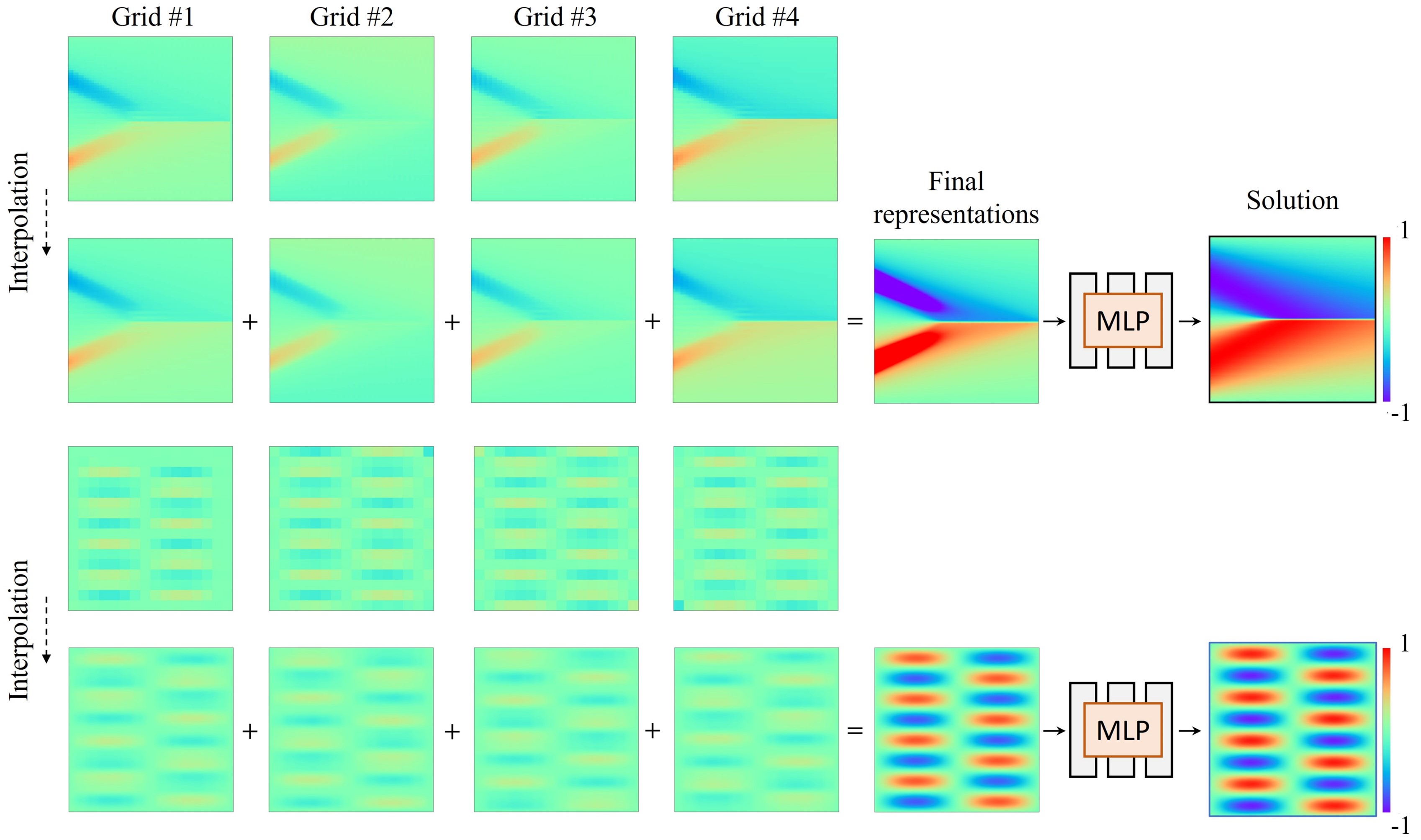
Figure 6: Visualization of multigrid representations for Burgers and Helmholtz equations (best viewed zoomed in): The first row shows image plots of each grid representation, and the second row shows the representations after the interpolation. The final representations are obtained through the sum of each interpolated cell, followed by an MLP to generate the solution. We used (4,4,64,64) and (4,4,16,16) multigrid representations for Burgers and Helmholtz, respectively.

We demonstrate the intermediate results in Figure 6. In Burgers example (the first and the second rows), we used (4,1,64,64) configuration and two layers of MLP with 16 hidden units. As we expect, each grid show foggy images since the final solution will be the sum of all multigrid representations. Also, we shifted each grid, which resulted in slightly different images from each other. The final solution is completed in the last stage by filling up the remaining contents using an MLP. Importantly, we note that the singular behavior (shock, a thin line in the middle of the solution image) is already well captured by the grid representations. The role of MLP was to represent the smooth global component in solution function. Therefore, the proposed grid representations and an MLP combine each other’s strengths to obtain better final solutions.

In Helmholtz example, we used small size grids (4,4,16,16). Thus, we can observe notable differences after cosine interpolation (grid-like pattern before the interpolation). We also note that the grid representations already represent complex patterns, and the last MLP stage also refined the solution by darkening the colors in the solution image.

Appendix D Data

We used publicly available data from (Raissi, Perdikaris, and Karniadakis 2019), which is the ground truh data for Burgers and Allen-Cahn equations.

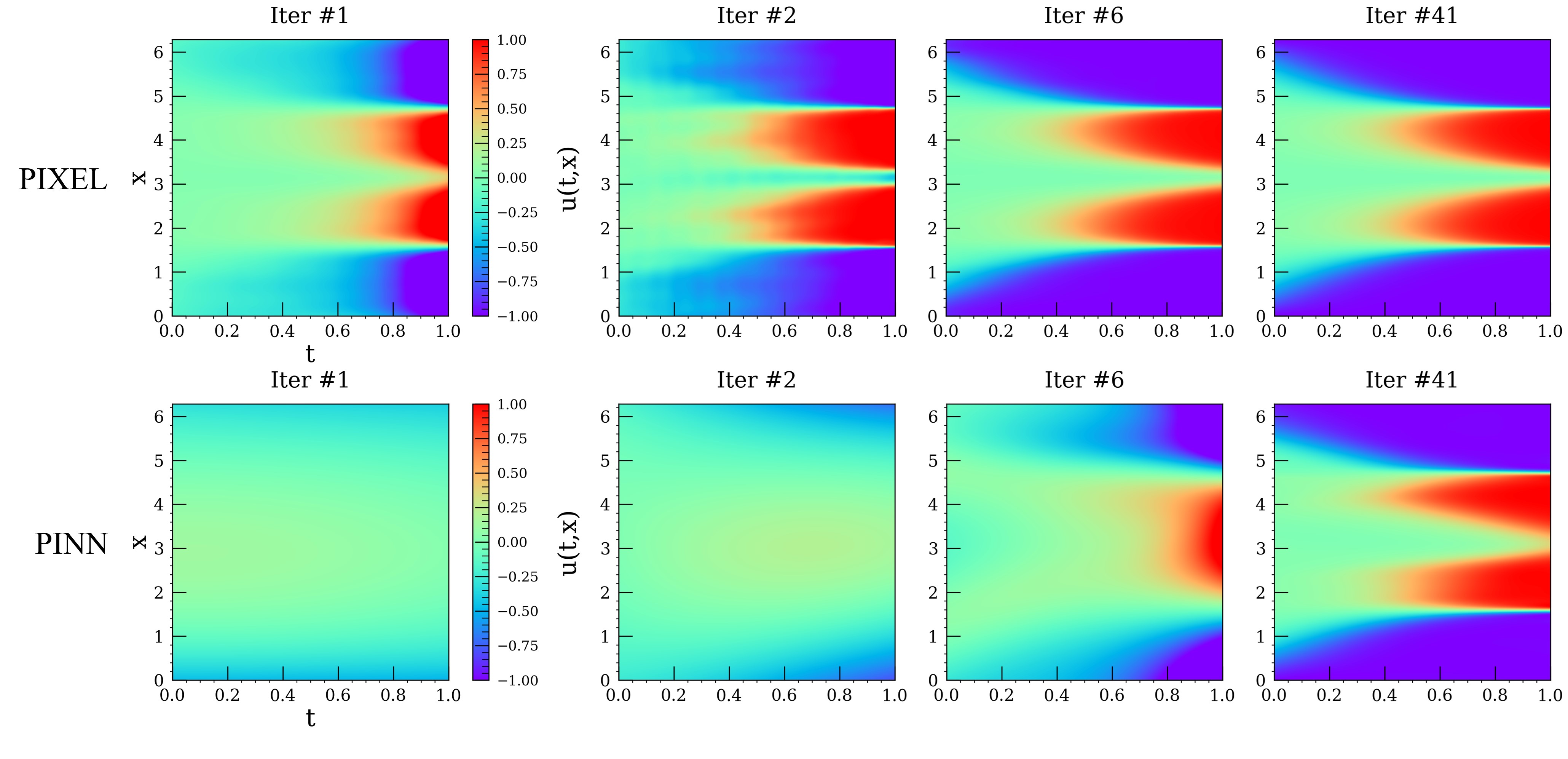
Figure 7: Inverse problem of allen-cahn equation

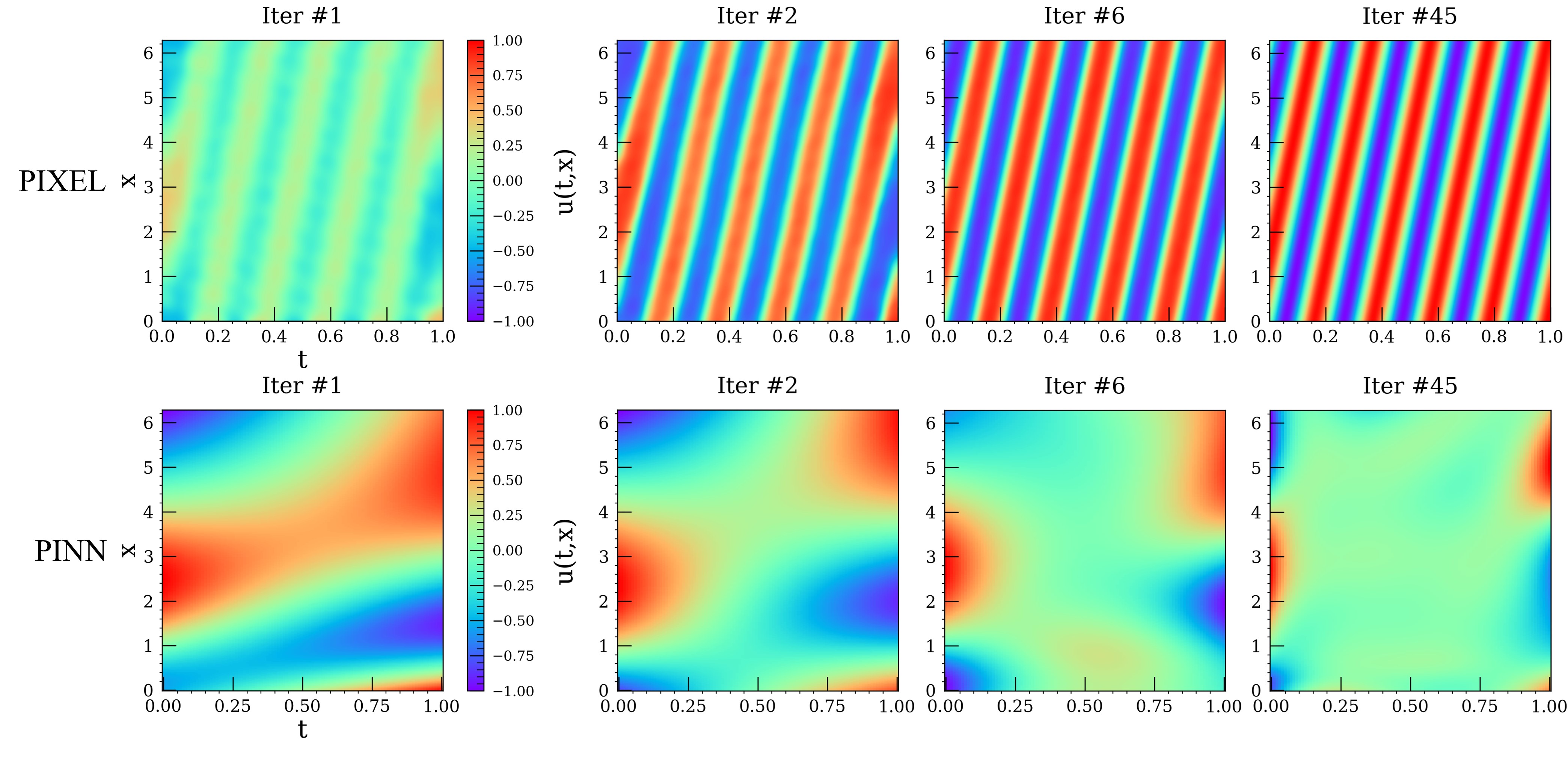
Figure 8: Inverse problem of convection equation

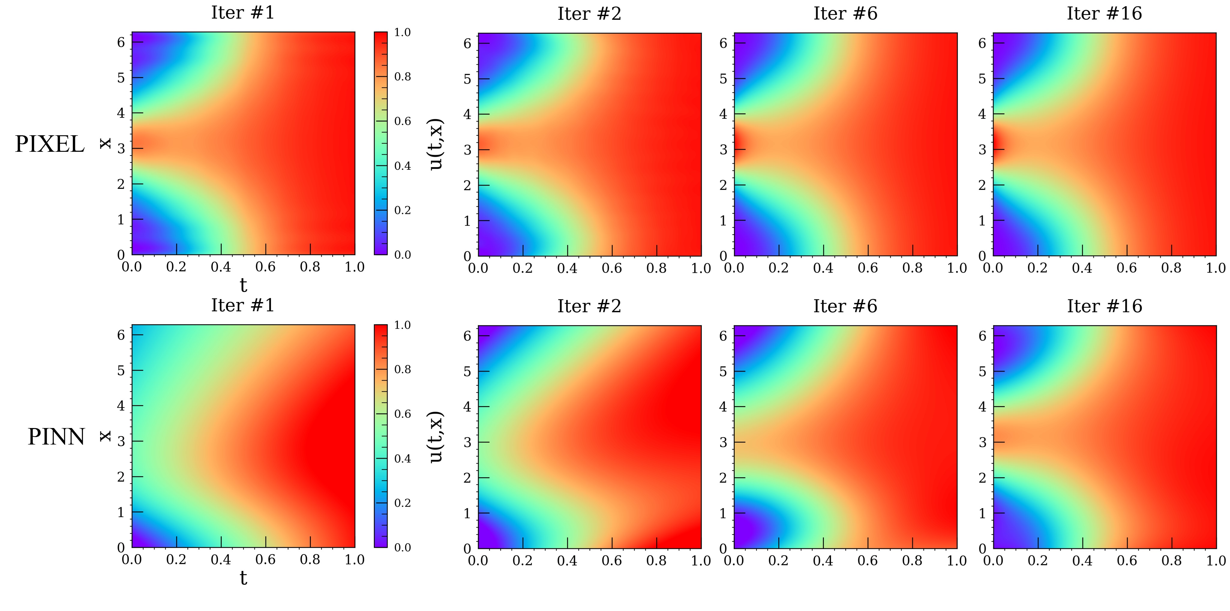
Figure 9: Inverse problem of reaction-diffusion equation

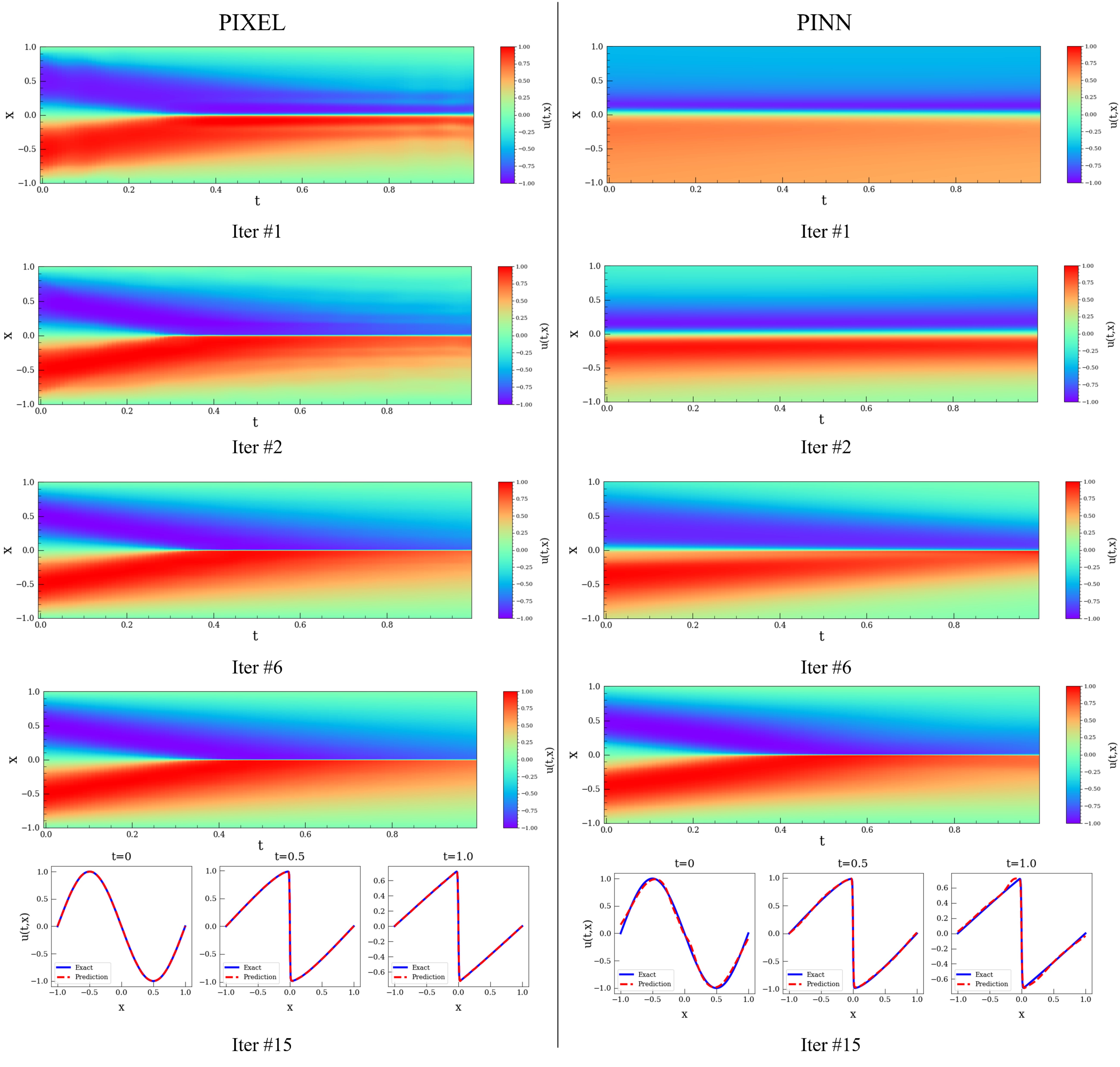
Figure 10: Inverse problem of burgers equation

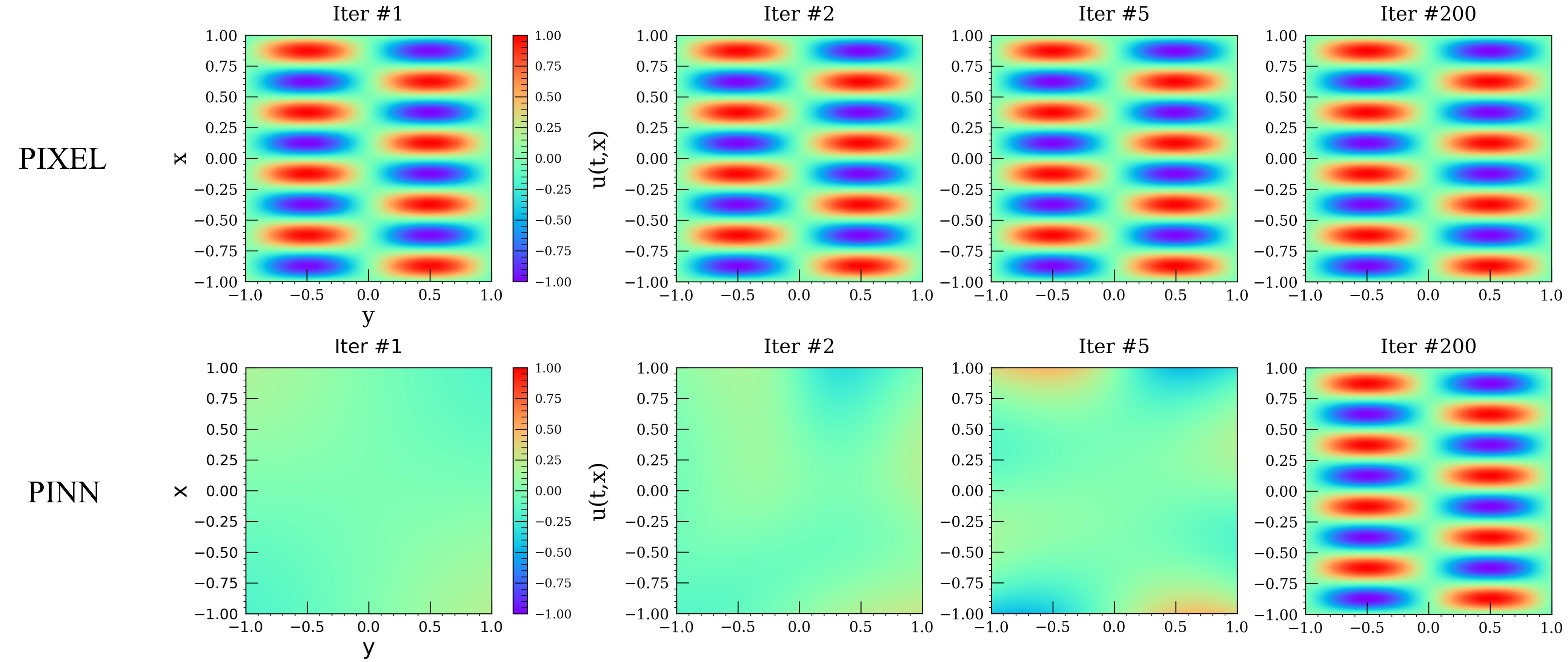
Figure 11: Inverse problem of helmholtz equation.

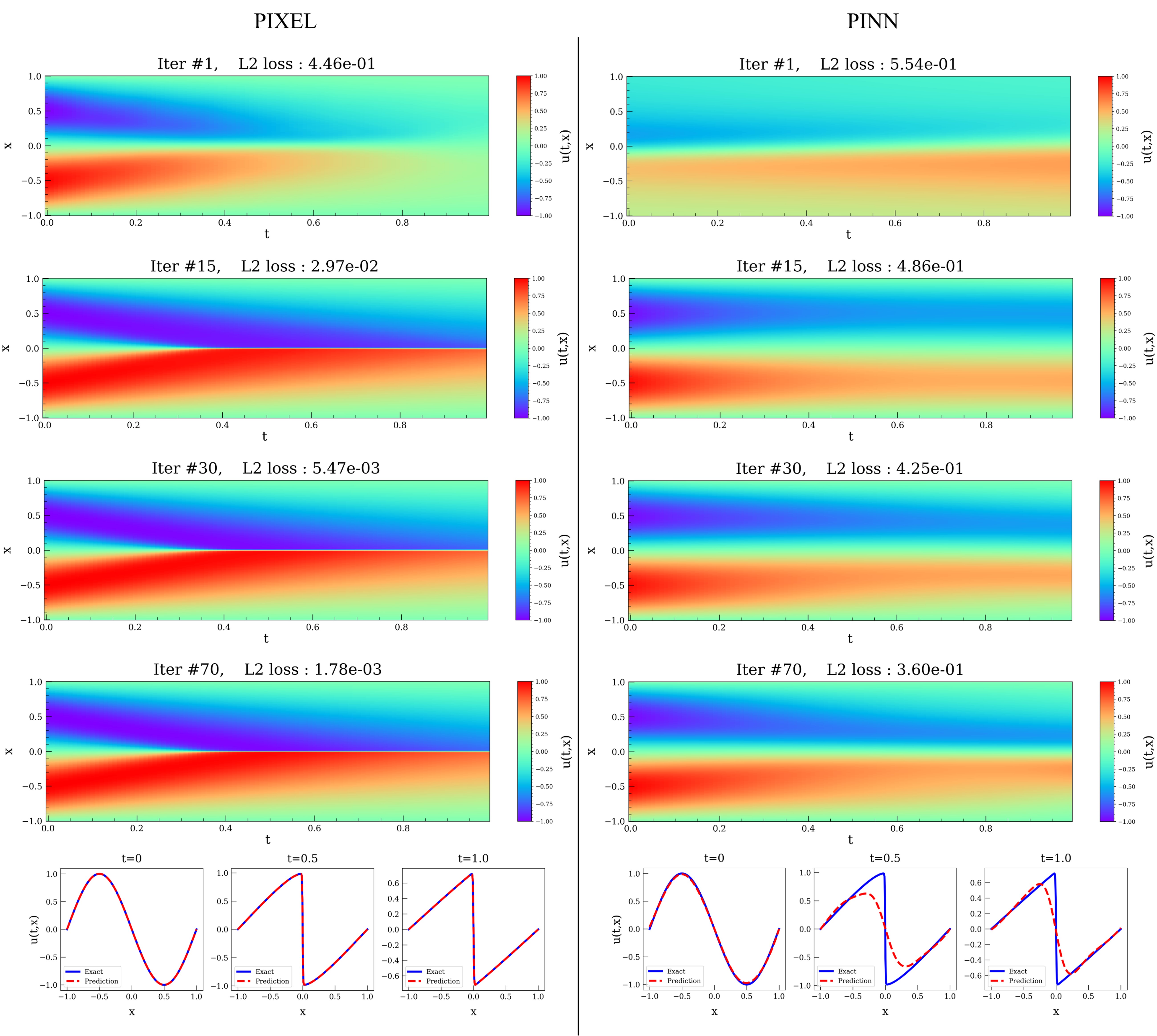
Figure 12: Forward problem of burgers equation

Figure 13: Convection equation results of PIXEL, at the 1500 iteration, the final relative $L_{2}$ error is 2.69e-03

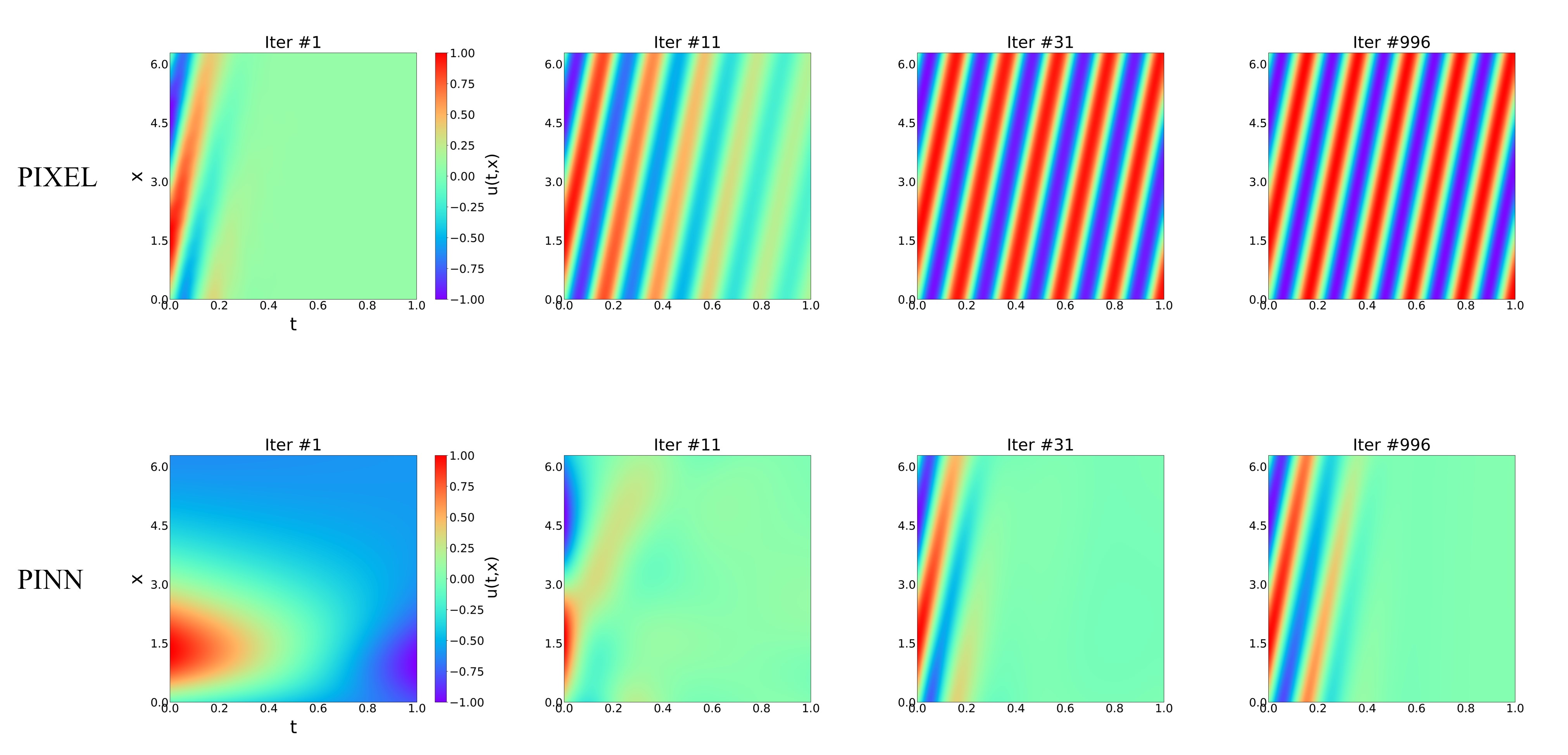
Figure 14: Forward problem of convection equation

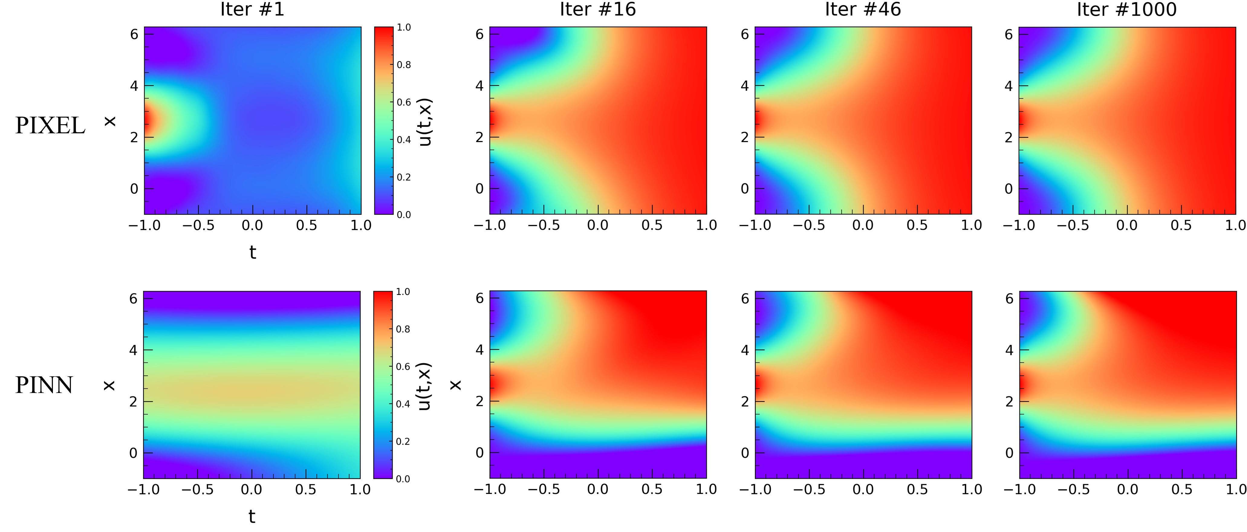
Figure 15: Forward problem of reaction-diffusion equation

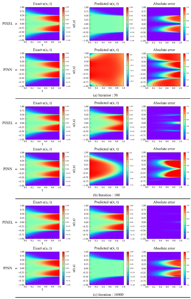
Figure 16: Forward problem of allen-cahn equation.

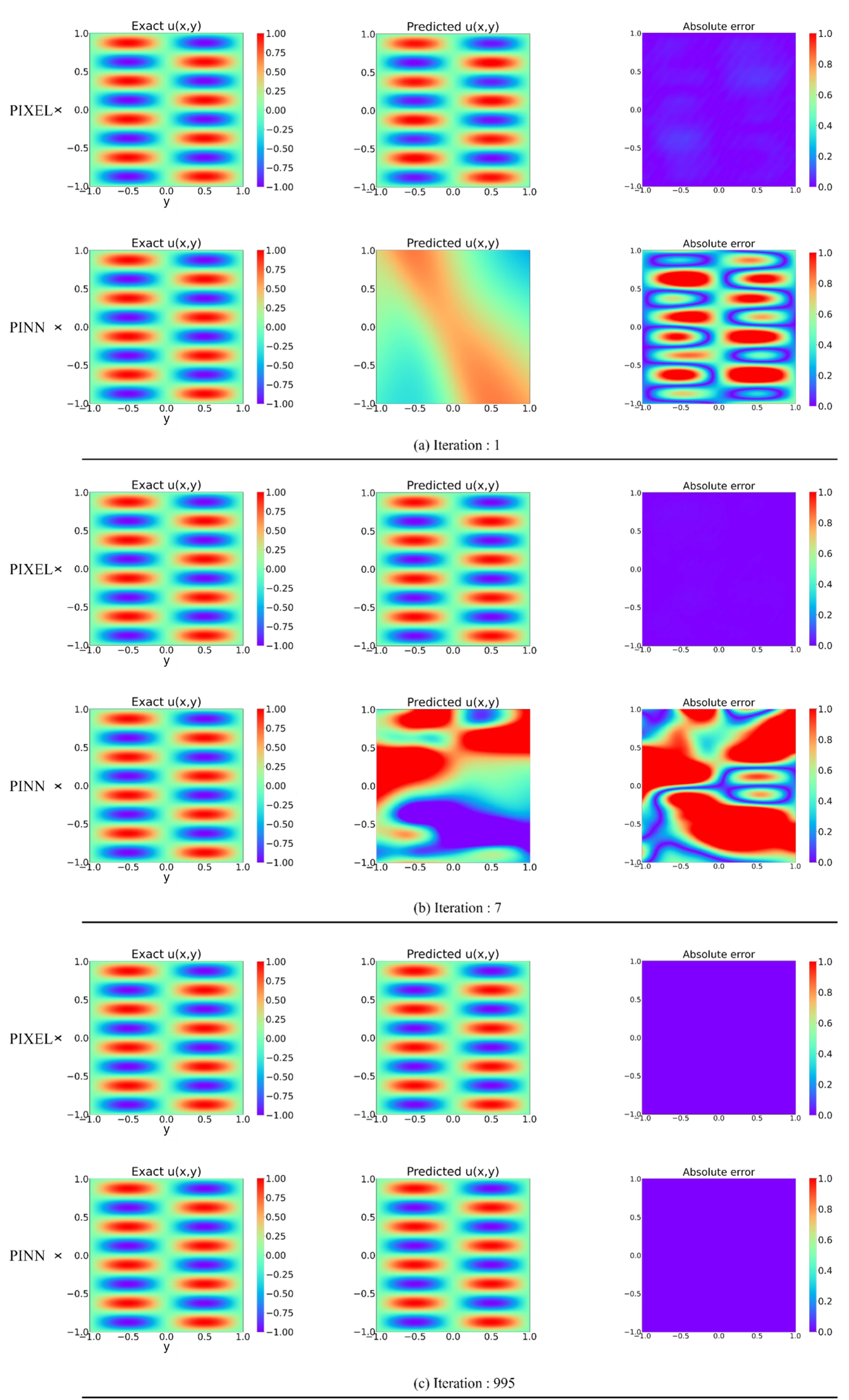
Figure 17: Forward problem of helmholtz equation

aaai23_

References

- Baydin et al. (2018) Baydin, A. G.; Pearlmutter, B. A.; Radul, A. A.; and Siskind, J. M. 2018. Automatic differentiation in machine learning: a survey. Journal of Marchine Learning Research, 18: 1–43.
- Chen et al. (2022) Chen, A.; Xu, Z.; Geiger, A.; Yu, J.; and Su, H. 2022. TensoRF: Tensorial Radiance Fields. In European Conference on Computer Vision (ECCV).
- Chen, Liu, and Wang (2021) Chen, Y.; Liu, S.; and Wang, X. 2021. Learning continuous image representation with local implicit image function. In Proceedings of the IEEE/CVF Conference on Computer Vision and Pattern Recognition, 8628–8638.
- Chibane, Alldieck, and Pons-Moll (2020) Chibane, J.; Alldieck, T.; and Pons-Moll, G. 2020. Implicit functions in feature space for 3d shape reconstruction and completion. In Proceedings of the IEEE/CVF Conference on Computer Vision and Pattern Recognition, 6970–6981.
- Dai et al. (2017) Dai, J.; Qi, H.; Xiong, Y.; Li, Y.; Zhang, G.; Hu, H.; and Wei, Y. 2017. Deformable convolutional networks. In Proceedings of the IEEE international conference on computer vision, 764–773.
- Evans (2010) Evans, L. C. 2010. Partial differential equations, volume 19. American Mathematical Soc.
- Eymard, Gallouët, and Herbin (2000) Eymard, R.; Gallouët, T.; and Herbin, R. 2000. Finite volume methods. Handbook of numerical analysis, 7: 713–1018.
- Fathi et al. (2020) Fathi, M. F.; Perez-Raya, I.; Baghaie, A.; Berg, P.; Janiga, G.; Arzani, A.; and D’Souza, R. M. 2020. Super-resolution and denoising of 4D-Flow MRI using physics-informed deep neural nets. Computer Methods and Programs in Biomedicine, 197: 105729.
- Fridovich-Keil et al. (2022) Fridovich-Keil, S.; Yu, A.; Tancik, M.; Chen, Q.; Recht, B.; and Kanazawa, A. 2022. Plenoxels: Radiance Fields Without Neural Networks. In Proceedings of the IEEE/CVF Conference on Computer Vision and Pattern Recognition (CVPR), 5501–5510.
- Girshick (2015) Girshick, R. 2015. Fast r-cnn. In Proceedings of the IEEE international conference on computer vision, 1440–1448.
- Guo, Li, and Iorio (2016) Guo, X.; Li, W.; and Iorio, F. 2016. Convolutional neural networks for steady flow approximation. In Proceedings of the 22nd ACM SIGKDD international conference on knowledge discovery and data mining, 481–490.
- He et al. (2017) He, K.; Gkioxari, G.; Dollár, P.; and Girshick, R. 2017. Mask r-cnn. In Proceedings of the IEEE international conference on computer vision, 2961–2969.
- Ioffe and Szegedy (2015) Ioffe, S.; and Szegedy, C. 2015. Batch normalization: Accelerating deep network training by reducing internal covariate shift. In International conference on machine learning, 448–456. PMLR.
- Jaderberg et al. (2015) Jaderberg, M.; Simonyan, K.; Zisserman, A.; and Kavukcuoglu, K. 2015. Spatial Transformer Networks. In Advances in Neural Information Processing Systems.
- Kingma and Ba (2014) Kingma, D. P.; and Ba, J. 2014. Adam: A Method for Stochastic Optimization. arXiv:1412.6980.
- Kolda and Bader (2009) Kolda, T. G.; and Bader, B. W. 2009. Tensor decompositions and applications. SIAM Review, 51(3): 455–500.
- Krishnapriyan et al. (2021) Krishnapriyan, A.; Gholami, A.; Zhe, S.; Kirby, R.; and Mahoney, M. W. 2021. Characterizing possible failure modes in physics-informed neural networks. Advances in Neural Information Processing Systems, 34.
- Le Gall (1991) Le Gall, D. 1991. MPEG: A video compression standard for multimedia applications. Communications of the ACM, 34(4): 46–58.
- Li et al. (2020) Li, Z.; Kovachki, N.; Azizzadenesheli, K.; Liu, B.; Bhattacharya, K.; Stuart, A.; and Anandkumar, A. 2020. Neural Operator: Graph Kernel Network for Partial Differential Equations. arXiv:2003.03485.
- Li et al. (2021a) Li, Z.; Kovachki, N. B.; Azizzadenesheli, K.; Liu, B.; Bhattacharya, K.; Stuart, A. M.; and Anandkumar, A. 2021a. Fourier Neural Operator for Parametric Partial Differential Equations. In 9th International Conference on Learning Representations, ICLR 2021, Virtual Event, Austria, May 3-7, 2021.
- Li et al. (2021b) Li, Z.; Zheng, H.; Kovachki, N.; Jin, D.; Chen, H.; Liu, B.; Azizzadenesheli, K.; and Anandkumar, A. 2021b. Physics-Informed Neural Operator for Learning Partial Differential Equations. arXiv:2111.03794.
- Liu and Wang (2021) Liu, D.; and Wang, Y. 2021. A Dual-Dimer method for training physics-constrained neural networks with minimax architecture. Neural Networks, 136: 112–125.
- Liu and Nocedal (1989) Liu, D. C.; and Nocedal, J. 1989. On the limited memory BFGS method for large scale optimization. Mathematical programming, 45(1): 503–528.
- Lu et al. (2020) Lu, L.; Dao, M.; Kumar, P.; Ramamurty, U.; Karniadakis, G. E.; and Suresh, S. 2020. Extraction of mechanical properties of materials through deep learning from instrumented indentation. Proceedings of the National Academy of Sciences, 117(13): 7052–7062.
- Lu et al. (2021) Lu, L.; Jin, P.; Pang, G.; Zhang, Z.; and Karniadakis, G. E. 2021. Learning nonlinear operators via DeepONet based on the universal approximation theorem of operators. Nature Machine Intelligence, 3(3): 218–229.
- Maclaurin, Duvenaud, and Adams (2015) Maclaurin, D.; Duvenaud, D.; and Adams, R. P. 2015. Autograd: Effortless gradients in numpy. In ICML 2015 AutoML workshop, volume 238.
- Martel et al. (2021) Martel, J. N.; Lindell, D. B.; Lin, C. Z.; Chan, E. R.; Monteiro, M.; and Wetzstein, G. 2021. Acorn: adaptive coordinate networks for neural scene representation. ACM Transactions on Graphics (TOG), 40(4): 1–13.
- Mattey and Ghosh (2022) Mattey, R.; and Ghosh, S. 2022. A novel sequential method to train physics informed neural networks for Allen Cahn and Cahn Hilliard equations. Computer Methods in Applied Mechanics and Engineering, 390: 114474.
- McClenny and Braga-Neto (2020) McClenny, L.; and Braga-Neto, U. 2020. Self-Adaptive Physics-Informed Neural Networks using a Soft Attention Mechanism. arXiv:2009.04544.
- Mekchay and Nochetto (2005) Mekchay, K.; and Nochetto, R. H. 2005. Convergence of adaptive finite element methods for general second order linear elliptic PDEs. SIAM Journal on Numerical Analysis, 43(5): 1803–1827.
- Meng et al. (2020) Meng, X.; Li, Z.; Zhang, D.; and Karniadakis, G. E. 2020. PPINN: Parareal physics-informed neural network for time-dependent PDEs. Computer Methods in Applied Mechanics and Engineering, 370: 113250.
- Moseley, Markham, and Nissen-Meyer (2021) Moseley, B.; Markham, A.; and Nissen-Meyer, T. 2021. Finite Basis Physics-Informed Neural Networks (FBPINNs): a scalable domain decomposition approach for solving differential equations. arXiv:2107.07871.
- Müller et al. (2022) Müller, T.; Evans, A.; Schied, C.; and Keller, A. 2022. Instant neural graphics primitives with a multiresolution hash encoding. ACM Transactions on Graphics, 41(4): 1–15.
- Nochetto et al. (2009) Nochetto, R. H.; Siebert, K. G.; ; and Veeser, A. 2009. Theory of adaptive finite element methods: An introduction. Multiscale, Nonlinear and Adaptive Approximation, 409–542.
- Park et al. (2019) Park, J. J.; Florence, P.; Straub, J.; Newcombe, R.; and Lovegrove, S. 2019. Deepsdf: Learning continuous signed distance functions for shape representation. In Proceedings of the IEEE/CVF Conference on Computer Vision and Pattern Recognition, 165–174.
- Paszke et al. (2017) Paszke, A.; Gross, S.; Chintala, S.; Chanan, G.; Yang, E.; DeVito, Z.; Lin, Z.; Desmaison, A.; Antiga, L.; and Lerer, A. 2017. Automatic differentiation in pytorch. Autodiff Workshop on Advances in Neural Information Processing Systems.
- Pedersoli et al. (2017) Pedersoli, M.; Lucas, T.; Schmid, C.; and Verbeek, J. 2017. Areas of attention for image captioning. In Proceedings of the IEEE international conference on computer vision, 1242–1250.
- Prato Torres, Domínguez, and Díaz (2019) Prato Torres, R.; Domínguez, C.; and Díaz, S. 2019. An adaptive finite element method for a time-dependent Stokes problem. Numerical Methods for Partial Differential Equations, 35(1): 325–348.
- Rahaman et al. (2019) Rahaman, N.; Baratin, A.; Arpit, D.; Draxler, F.; Lin, M.; Hamprecht, F.; Bengio, Y.; and Courville, A. 2019. On the spectral bias of neural networks. In International Conference on Machine Learning, 5301–5310. PMLR.
- Raissi (2018) Raissi, M. 2018. Deep hidden physics models: Deep learning of nonlinear partial differential equations. The Journal of Machine Learning Research, 19(1): 932–955.
- Raissi, Perdikaris, and Karniadakis (2019) Raissi, M.; Perdikaris, P.; and Karniadakis, G. E. 2019. Physics-informed neural networks: A deep learning framework for solving forward and inverse problems involving nonlinear partial differential equations. Journal of Computational physics, 378: 686–707.
- Reiser et al. (2021) Reiser, C.; Peng, S.; Liao, Y.; and Geiger, A. 2021. Kilonerf: Speeding up neural radiance fields with thousands of tiny mlps. In Proceedings of the IEEE/CVF International Conference on Computer Vision, 14335–14345.
- Rudy et al. (2017) Rudy, S. H.; Brunton, S. L.; Proctor, J. L.; and Kutz, J. N. 2017. Data-driven discovery of partial differential equations. Science advances, 3(4): e1602614.
- Sitzmann et al. (2020) Sitzmann, V.; Martel, J.; Bergman, A.; Lindell, D.; and Wetzstein, G. 2020. Implicit neural representations with periodic activation functions. Advances in Neural Information Processing Systems, 33: 7462–7473.
- Smith (1985) Smith, G. D. 1985. Numerical solution of partial differential equations: finite difference methods. Oxford university press.
- Sun, Sun, and Chen (2022) Sun, C.; Sun, M.; and Chen, H.-T. 2022. Direct Voxel Grid Optimization: Super-Fast Convergence for Radiance Fields Reconstruction. In Proceedings of the IEEE/CVF Conference on Computer Vision and Pattern Recognition (CVPR), 5459–5469.
- Takikawa et al. (2021) Takikawa, T.; Litalien, J.; Yin, K.; Kreis, K.; Loop, C.; Nowrouzezahrai, D.; Jacobson, A.; McGuire, M.; and Fidler, S. 2021. Neural Geometric Level of Detail: Real-time Rendering with Implicit 3D Shapes. In IEEE Conference on Computer Vision and Pattern Recognition, CVPR, 11358–11367.
- Wallace (1992) Wallace, G. 1992. The JPEG still picture compression standard. IEEE Transactions on Consumer Electronics, 38(1): xviii–xxxiv.
- Wang, Bleja, and Agapito (2022) Wang, J.; Bleja, T.; and Agapito, L. 2022. Go-surf: Neural feature grid optimization for fast, high-fidelity rgb-d surface reconstruction. arXiv preprint arXiv:2206.14735.
- Wang, Sankaran, and Perdikaris (2022) Wang, S.; Sankaran, S.; and Perdikaris, P. 2022. Respecting causality is all you need for training physics-informed neural networks. arXiv:2203.07404.
- Wang, Teng, and Perdikaris (2021) Wang, S.; Teng, Y.; and Perdikaris, P. 2021. Understanding and mitigating gradient flow pathologies in physics-informed neural networks. SIAM Journal on Scientific Computing, 43(5): A3055–A3081.
- Wang, Wang, and Perdikaris (2021a) Wang, S.; Wang, H.; and Perdikaris, P. 2021a. Learning the solution operator of parametric partial differential equations with physics-informed DeepONets. Science advances, 7(40): eabi8605.
- Wang, Wang, and Perdikaris (2021b) Wang, S.; Wang, H.; and Perdikaris, P. 2021b. On the eigenvector bias of fourier feature networks: From regression to solving multi-scale pdes with physics-informed neural networks. Computer Methods in Applied Mechanics and Engineering, 384: 113938.
- Wang, Yu, and Perdikaris (2022) Wang, S.; Yu, X.; and Perdikaris, P. 2022. When and why PINNs fail to train: A neural tangent kernel perspective. Journal of Computational Physics, 449: 110768.
- Wight and Zhao (2020) Wight, C. L.; and Zhao, J. 2020. Solving Allen-Cahn and Cahn-Hilliard Equations using the Adaptive Physics Informed Neural Networks. arXiv:2007.04542.
- Xie et al. (2022) Xie, Y.; Takikawa, T.; Saito, S.; Litany, O.; Khan, S. Y. N.; Tombari, F.; Tompkin, J.; Sitzmann, V.; and Sridhar, S. 2022. Neural Fields in Visual Computing and Beyond. STAR, 41(2).
- Yuan et al. (2022) Yuan, L.; Ni, Y.-Q.; Deng, X.-Y.; and Hao, S. 2022. A-PINN: Auxiliary physics informed neural networks for forward and inverse problems of nonlinear integro-differential equations. Journal of Computational Physics, 111260.
- Zhu and Zabaras (2018) Zhu, Y.; and Zabaras, N. 2018. Bayesian deep convolutional encoder–decoder networks for surrogate modeling and uncertainty quantification. Journal of Computational Physics, 366: 415–447.
- Zienkiewicz, Taylor, and Zhu (2005) Zienkiewicz, O. C.; Taylor, R. L.; and Zhu, J. Z. 2005. The finite element method: its basis and fundamentals. Elsevier.