New developments in relativistic magnetohydrodynamics

Abstract

Relativistic magnetohydrodynamics (RMHD) provides an extremely useful description of the low-energy long-wavelength phenomena in a variety of physical systems from quark-gluon plasma in heavy-ion collisions to matters in supernova, compact stars, and early universe. We review the recent theoretical progresses of RMHD, such as a formulation of RMHD from the perspective of magnetic flux conservation using the entropy-current analysis, the nonequilibrium statistical operator approach applied to quantum electrodynamics, and the relativistic kinetic theory. We discuss how the transport coefficients in RMHD are computed in kinetic theory and perturbative quantum field theories. We also explore the collective modes and instabilities in RMHD with a special emphasis on the role of chirality in a parity-odd plasma. We also give some future prospects of RMHD, including the interaction with spin hydrodynamics and the new kinetic framework with magnetic flux conservation.

I Introduction

Relativistic hydrodynamics provides an incredibly successful description of the macroscopic dynamics of interacting many-body systems in relativistic arena since its birth Eckart (1940); Kluitenberg et al. (1953a, b); Kluitenberg and De Groot (1954a); Landau and Lifshitz (1959). Its applicability ranges from very small systems such as the quark gluon plasma (QGP) created in high-energy heavy-ion collisions to very large systems like the expanding universe and the explosive supernovas Yagi et al. (2008); Romatschke and Romatschke (2019). From a theoretical point of view, relativistic hydrodynamics is a typical example of effective field theories which is valid at low-energy and long-wavelength limit. The dynamical variables in relativistic hydrodynamics are the coarse-grained conserved quantities stemmed from the underlying symmetries. As such, there exist a variety of ways to systematically construct relativistic hydrodynamics when an appropriate derivative expansion is employed.

Strong magnetic fields exist and play critical roles in a number of systems where the relativistic hydrodynamics can be applied. Examples range from high-energy heavy-ion collisions to supernovas, neutron stars, and the early universe. In heavy-ion collisions, the colliding nuclei induce very strong transient magnetic fields exerting on the produced quark-gluon plasma (QGP) Skokov et al. (2009); Voronyuk et al. (2011); Bzdak and Skokov (2012); Deng and Huang (2012); Bloczynski et al. (2013); Tuchin (2013a); Yan and Huang (2021); Wang et al. (2022). The peak strength of such magnetic fields can reach $10^{19}$ Gauss in Au + Au collisions at Relativistic Heavy Ion Collider (RHIC) and $10^{20}$ Gauss in Pb + Pb collisions at Large Hadron Collider (LHC). Given that the QGP is also an electromagnetic (EM) plasma, such magnetic fields can strongly influence the dynamics of QGP and induce novel transport phenomena in QGP such as the chiral magnetic effect which provides a valuable machinery to access the quantum chromodynamics (QCD) topological sector in an experimentally feasible way Kharzeev et al. (2008); Fukushima et al. (2008). (For reviews of strong magnetic-field effects in heavy-ion collisions, see Refs. Miransky and Shovkovy (2015); Huang (2016); Hattori and Huang (2017); Kharzeev et al. (2016); Kharzeev and Liao (2021).)

In compact stellar objects such as the neutron stars, the surface magnetic fields can reach the order of $10^{12}–10^{13}$ Gauss Shapiro and Teukolsky (1983), with a subclass of neutron stars (called magnetars) having surface magnetic fields of the order of $10^{14}–10^{15}$ Gauss Duncan and Thompson (1992) (Even stronger transient magnetic fields may be created in binary neutron star mergers Price and Rosswog (2006); Kiuchi et al. (2015)). The internal magnetic fields could be by orders of magnitude stronger than the surface magnetic fields. Although the origin of magnetar magnetic fields is not fully understood, one widely accepted theory is that they result from the magnetohydrodynamic dynamo processes in the interior fluids of some newly born neutron stars Thompson and Duncan (1993). Observationally, soft gamma ray repeaters (SGRs) and anomalous X-ray pulsars (AXPs) are commonly identified as magnetars. The strong magnetic fields are crucial for understanding the phenomenology of neutron stars, particularly magnetars, such as radio emission, cooling properties, equations of state, shape deformation and gravitational-wave emission, merging processes and post-merger evolution of binary neutron stars, among other things. (See Refs. Lai (2001); Harding and Lai (2006); Mereghetti et al. (2015); Turolla et al. (2015); Kaspi and Beloborodov (2017); Enoto et al. (2019); Ciolfi (2020) for reviews.)

Although a conclusive evidence for primordial magnetic fields in the early universe is still lacking, astrophysical studies of the large-scale intergalactic magnetic fields in the current universe strongly support their existence. The origin of the primordial magnetic fields has been pursued over the last three decades with possible scenarios stemming from the big-bang era Turner and Widrow (1988); Carroll et al. (1990); Garretson et al. (1992) and cosmic phase transitions like the QCD phase transition and the electroweak phase transition Hogan (1983); Quashnock et al. (1989); Vachaspati (1991); Cheng and Olinto (1994); Baym et al. (1996); Son (1999). Besides, the strong primordial magnetic fields may have played an important role in understanding the cosmological structure formation, the thermal spectrum and polarization anisotropies of the cosmic microwave background, the big-bang nucleosynthesis and baryogenesis, and so on. (For reviews of the primordial magnetic fields, see Refs. Grasso and Rubinstein (2001); Kandus et al. (2011); Subramanian (2016).)

The relativistic magnetohydrodynamics (relativistic MHD or RMHD) is often used as a standard tool to analyze the physical processes in the systems mentioned above. It provides a macroscopic framework to self-consistently describe the evolution of the matter coupled with either dynamical electromagnetic (EM) fields or in external EM fields. There is a long history of astrophysical and cosmological applications of RMHD (typically in the presence of gravity), and there are already a number of excellent reviews and textbooks (see, for example, books Lichnerowicz (1994); Anile (2005); Rezzolla and Zanotti (2013); Goedbloed et al. (2019); Kato and Fukue (2020)). Over the last decade, due to the realization of strong magnetic fields in heavy ion collisions, various aspects and applications of RMHD in the context of heavy ion collisions have been extensively investigated, including the study of evolution of magnetic fields in the QGP Tuchin (2013b); Li et al. (2016), the computation of RMHD transport coefficients in QCD matter using perturbative field theory Hattori et al. (2017a); Hattori and Satow (2016); Hattori et al. (2017b, c); Li and Yee (2018), kinetic theories Denicol et al. (2018, 2019); Dey et al. (2021a); Chen et al. (2020); Dash et al. (2020); Singh et al. (2020); Panda et al. (2021a); Ghosh and Haque (2022), and holographic models Critelli et al. (2014); Finazzo et al. (2016); Li et al. (2018); Fukushima and Okutsu (2022), the anisotropic evolution of the QGP coupled with magnetic fields Tuchin (2012); Gursoy et al. (2014); Roy et al. (2015); Pu and Yang (2016); Pu et al. (2016); Inghirami et al. (2016); Gürsoy et al. (2018); She et al. (2019); Inghirami et al. (2020); Kord et al. (2022); Emamian et al. (2020), the simulation of chiral magnetic effect and other anomalous transport phenomena Hongo et al. (2017); Yee and Yin (2014); Hirono et al. (2014); Yin and Liao (2016); Huang et al. (2016); Jiang et al. (2018); Shi et al. (2018); Guo et al. (2017); Shi et al. (2020); Siddique et al. (2019), among other things. In particular, the presence of the axial charge induced by a topological nature of the system motivated people to extend RMHD to the chiral magnetohydrodynamics (chiral MHD) Hattori et al. (2019a), which gives a potential theoretical tool to investigate the dynamical origin of the primordial large-scale magnetic field Tashiro et al. (2012); Boyarsky et al. (2015); Rogachevskii et al. (2017); Schober et al. (2018); Brandenburg et al. (2017); Boyarsky et al. (2021) (see also Refs. Joyce and Shaposhnikov (1997); Field and Carroll (2000); Giovannini (2004); Semikoz and Sokoloff (2005); Laine (2005); Boyarsky et al. (2012) for earlier approaches to this problem based on RMHD).

Instead of exploring into the details of RMHD applications in many subfields of physics, the goal of this article is to present a two-fold overview of the theoretical aspects of the special relativistic MHD: One based on the recent formulation of RMHD motivated by the generalized symmetry viewpoint, and the other with the conventional approach in which the matter components and the EM fields are separated discussed. We will present our view to relate these two formulations with each other.

As a branch of relativistic hydrodynamics, the RMHD can also be considered as an effective theory of low-energy long-wavelength modes of the system. Such modes are usually the conserved modes like the energy and momentum modes. When the EM fields are dynamical, it has been suggested recently that the Bianchi identity for EM fields can be regarded as a conservation law (associated with a one-form magnetic $U(1)$ symmetry) Grozdanov et al. (2017); Hattori et al. (2019a); Glorioso and Son (2018); Armas and Jain (2019, 2020); Hongo and Hattori (2021), allowing a formulation of RMHD based solely on symmetry argument and derivative expansions of conserved quantities (in this case, called hydrodynamic variables) . We will give detailed discussion about the construction of RMHD in this manner in Sec. II using a phenomenological method based on entropy-current analysis and in Sec. III using a nonequilibrium statistical operator method. A crucial observation of such a construction is that the magnetic field, like temperature and fluid velocity, persists at thermal equilibrium and can thus be assigned as a leading-order variable in derivative expansion. This is known as a strong magnetic field, and is the scenario that we are concerned with . As a result, the constitutive relations exhibit anisotropies at both the ideal and dissipative levels, which is a distinguished feature of RMHD (also non-relativistic MHD, in fact) Braginskii (1965); Lifschitz and Pitaevskii (1981); Huang et al. (2010, 2011); Hernandez and Kovtun (2017).

We will then examine how this new formulation is connected to the conventional approach in Sec. IV, and proceed with the evaluations of transport coefficients in kinetic theory and in perturbative quantum field theories (QED, as an example) in Sec. V and Sec. VI, respectively. More novel features can appear in RMHD when the system allows parity violation, leading to the chiral MHD. This will be explored in Sec. VII. We note that there is an significant difference between the treatments of EM fields in Secs. II,  III,  VII and that in Secs. V and  VI. In Secs. II, III, and VII, we treat the EM fields as dynamical variables following a recent formulation of RMHD. On the other hand, the EM fields in Secs. V and  VI are considered as backgrounds, and formulations are closer to the conventional approach with the EM fields treated separately from the matter components. Considering this difference, we compare the result of Secs. II-III to the conventional one to clarify these two formulations in the intermediate section IV. Finally, we discuss the future prospects of RMHD in Sec. VIII.

Here is a summary of our notations. We use the natural units, $\hbar=c=k_{B}=1$. For the electromagnetism, we use the Heaviside-Lorentz convention $\epsilon_{0}=\mu_{0}=1$ and $\alpha=e^{2}/(4\pi)$=1/137. Other notations are:

• Minkowski metric: $\eta_{\mu\nu}=\eta^{\mu\nu}={\rm diag}(1,-1,-1,-1)$. A curved-spacetime metric is denoted by $g_{\mu\nu}$.

• Levi-Civita tensor in Minkowski spacetime: $\varepsilon^{\mu\nu\rho\sigma}$ with $\varepsilon^{0123}=-\varepsilon_{0123}=1$.

• Fluid velocity four vector: $u^{\mu}=\gamma\,(1,\bm{v})^{T}$ with $\gamma=1/\sqrt{1-\bm{v}^{2}}$ and $u^{2}=1$.

• Direction of the magnetic field: $b^{\mu}=B^{\mu}/B$ with $B=\sqrt{-B_{\mu}B^{\mu}}$. Note that $b^{2}=-1$ and $b\cdot u=0$.

• Projector transverse to $u^{\mu}$: $\Delta^{\mu\nu}=\eta^{\mu\nu}-u^{\mu}u^{\nu}$.

• Projector transverse to both $u^{\mu}$ and $b^{\mu}$: $\Xi^{\mu\nu}=\Delta^{\mu\nu}+b^{\mu}b^{\nu}$.

• Cross projector: $b_{\star}^{\mu\nu}=-b_{\star}^{\nu\mu}=\varepsilon^{\mu\nu\rho\sigma}u_{\rho}b_{\sigma}$. Note that $u_{\mu}b_{\star}^{\mu\nu}=0=b_{\mu}b_{\star}^{\mu\nu}$, $b_{\star}^{\mu\lambda}b^{\nu}_{\star\lambda}=\Xi^{\mu\nu}$.

• Co-moving derivative (or material derivative or proper-time derivative) of $A$: $DA=\dot{A}=dA/d\tau=u^{\mu}\partial_{\mu}A$.

• Spatial gradient of $A$: $\nabla_{\mu}A=\Delta_{\mu\nu}\partial^{\nu}A$.

• Symmetrization, anti-symmetrization, and traceless symmetrization of a rank-two tensor $A^{\mu\nu}$: $A^{(\mu\nu)}=(A^{\mu\nu}+A^{\nu\mu})/2$, $A^{[\mu\nu]}=(A^{\mu\nu}-A^{\nu\mu})/2$, and $A^{\langle\mu\nu\rangle}=(1/2)\Delta^{\mu}_{\alpha}\Delta^{\nu}_{\beta}(A^{\alpha\beta}+A^{\alpha\beta})-(1/3)\Delta^{\mu\nu}\Delta_{\alpha\beta}A^{\alpha\beta}$.

• Decomposition of velocity gradient: $\partial_{\mu}u_{\nu}=u_{\mu}Du_{\nu}+\omega_{\mu\nu}+w_{\mu\nu}$ where $\omega_{\mu\nu}=\nabla_{[\mu}u_{\nu]}$ is the vorticity tensor and $w_{\mu\nu}=\nabla_{(\mu}u_{\nu)}=\nabla_{\langle\mu}u_{\nu\rangle}+\frac{1}{3}\Delta_{\mu\nu}\theta$ with $\nabla_{\langle\mu}u_{\nu\rangle}$ the shear tensor and $\theta=\Delta_{\alpha\beta}w^{\alpha\beta}$ the expansion rate of the fluid.

II Macroscopic approach: the entropy-current analysis

In this section, we review a phenomenological way to derive the RMHD equations based on the second law of local thermodynamics. In Sec. II.1, we first give a brief overview of how one can build relativistic hydrodynamics without coupling to the EM fields before going into the discussion of RMHD. This can help us understand some basic ingredients that are essential to the construction of RMHD. In Sec. II.2, we generalize our discussion to RMHD based on the symmetry associated with the Bianchi identity.

As mentioned in Sec. I, hydrodynamics is regarded as a low-energy effective theory that describes the dynamics of gapless modes. In other words, hydrodynamics describes the macroscopic behavior of conserved charges that do not dissipate away. Therefore, it is crucial to identify symmetries of the system and associated conservation laws that serve as the equations of motion (EOMs) in hydrodynamics. This observation allows us to derive hydrodynamics from the viewpoint of the symmetry and thermodynamics of irreversible processes Landau and Lifshitz (1959); De Groot and Mazur (1962) without going into details of the system. This macroscopic (phenomenological) approach is often called the entropy-current analysis since the constitutive relations (see definition below Eq. (3)) are derived by requiring the semi-positivity of the entropy-current divergence, or the second law of local thermodynamics.

II.1 Primer to the entropy-current analysis

For the sake of simplicity, let us consider a relativistic system that only enjoys spacetime translational symmetries, and thus, respects the energy-momentum conservation law:

$$\partial_{\mu}T^{\mu\nu}=0,$$ (1)

where $T^{\mu\nu}$ denotes the energy-momentum tensor.Throughout this paper, we always consider relativistic systems respecting the Lorentz symmetry, so that one can write down the hydrodynamic equations in a Lorentz covariant manner. One may think that the Lorentz symmetry itself leads to the angular momentum conservation law, which should give independent hydrodynamic equations as well. However, in the strict hydrodynamic limit (i.e., the long wavelength and low frequency limit), the angular momentum conservation law reduces to the constraint equation that forces the energy-momentum tensor to be symmetric under the exchange of its two Lorentz indices. We thus use the symmetric energy-momentum tensor $T^{\mu\nu}=T^{\nu\mu}$ in the following discussion . We also note that the discrete charge-conjugation (C), time reversal (T), and parity (P) symmetries also impose strong constraints on the transport phenomena. As will be seen in Sec. VII, breaking one or two of them will allow the appearance of new transport terms in the constitutive relations. In this section, however, we assume that C, P, T symmetries are not violated.

Dynamical variables of hydrodynamics are the conserved energy-momentum densities, or the corresponding thermodynamic conjugate variables given by the fluid four-velocity $u^{\mu}$ — normalized as $\eta_{\mu\nu}u^{\mu}u^{\nu}=1$ with the Minkowski metric $\eta_{\mu\nu}=\mathrm{diag}(+1,-1,-1,-1)$ — and the local inverse temperature $\beta=1/T$. In this paper, we employ the Landau-Lifshitz frame Landau and Lifshitz (1959) to define the fluid velocity by

$$T^{\mu}_{~{}\nu}u^{\nu}=\epsilon u^{\nu},$$ (2)

with the energy density $\epsilon$. The local inverse temperature is related to the energy density $\epsilon$ through the usual thermodynamic relation. We will later give a concrete definition of the inverse temperature in Eq. (8) when we start to consider the entropy density.

Then, as a long-wavelength low-frequency effective theory, one can formulate hydrodynamics based on an expansion of $T^{\mu\nu}$ with respect to the small derivatives of $u^{\mu}$ and $\beta$ as

$$T^{\mu\nu}=T^{\mu\nu}_{(0)}+T^{\mu\nu}_{(1)}+O(\partial^{2}),$$ (3)

where the subscripts $(0)$ and $(1)$ denote numbers of derivatives. This equation, which expresses $T^{\mu\nu}$ in terms of the dynamical variable $u^{\mu}$ and $\beta$ (or $\epsilon$) is called the constitutive relation. We will construct the constitutive relation on an order-by-order basis.

In the leading-order derivative expansion, one can uniquely decompose the zeroth-order term $T^{\mu\nu}_{(0)}$ as

$$T^{\mu\nu}_{(0)}=\epsilon u^{\mu}u^{\nu}-p\Delta^{\mu\nu},$$ (4)

with the projection tensor $\Delta_{\mu\nu}=\eta_{\mu\nu}-u_{\mu}u_{\nu}$ satisfying $u^{\mu}\Delta_{\mu\nu}=0$. This is because no other rank-two symmetric tensors can be constructed from algebraic combinations of available building blocks $u^{\mu},\eta^{\mu\nu}$, and Levi-Civita tensor $\varepsilon^{\mu\nu\rho\sigma}$ (normalized to be $\varepsilon^{0123}=-\varepsilon_{0123}=1$). The scalar coefficient functions $\epsilon$ and $p$ are regarded as the energy density and pressure in the fluid rest frame. This interpretation becomes manifest, $T_{(0)}^{\mu\nu}={\rm diag}(\epsilon,p,p,p)$, when we take $u^{\mu}=(1,\bm{0})$. We note that we have already imposed the matching condition for $\epsilon$, $T^{\mu\nu}u_{\mu}u_{\nu}=T_{(0)}^{\mu\nu}u_{\mu}u_{\nu}$, in Eq. (4), which enforces that $T^{\mu\nu}_{(1)}u_{\nu}=0$ following Eqs. (2). On the other hand, no such matching condition is required for $p$, and there could be $O(\partial^{1})$ correction to the physical pressure in the fluid.

At this stage, Eq. (4) is just a parameterization of $T^{\mu\nu}_{(0)}$ using the unknown function $p$. In order to organize Eq. (1) in a solvable leading-order hydrodynamic equation with $T^{\mu\nu}_{(0)}$, we have to relate the pressure $p$ to $\epsilon$. If our system is close to the local thermal equilibrium, we can expect that such a relation is provided by the equation of state (EOS), $p=p(\epsilon)$, so that $p$ is identified as the thermodynamic pressure. As we will see shortly, $p(\epsilon)$ has to satisfy a certain thermodynamic relation in order to respect the second law of thermodynamics. Then, substituting the leading-order constitutive relation (4) into the conservation law (1), one obtains the relativistic Euler equations:

$$(\epsilon+p)Du^{\mu}-\nabla^{\mu}p=0\,,$$ (5a)

$$D\epsilon+(\epsilon+p)\theta=0\,,$$ (5b)

where we defined the material (or co-moving time) derivative $D=u^{\mu}\partial_{\mu}$, the spatial gradient $\nabla_{\mu}=\Delta_{\mu\nu}\partial^{\nu}$, and the expansion rate of the fluid $\theta=\partial_{\mu}u^{\mu}$.

In the same manner, we can continue to perform the tensor decomposition of the first-order term $T^{\mu\nu}_{(1)}$. Noting that $T^{\mu\nu}_{(1)}$ satisfies $T^{\mu\nu}_{(1)}u_{\nu}=0$ enforced by the Landau-Lifshitz frame condition and the matching condition for $\epsilon$, we use $\Delta^{\mu\nu}$ to decompose the rank-two symmetric tensor $T^{\mu\nu}_{(1)}$ into the trace part $\Pi$ and symmetric traceless part $\pi^{\mu\nu}$ (or $\pi^{\mu\nu}\Delta_{\mu\nu}=0$) as

$$T^{\mu\nu}_{(1)}=-\Delta^{\mu\nu}\Pi+\pi^{\mu\nu}.$$ (6)

This equation gives the decomposition of the rank-two symmetric tensor into irreducible representations of the $\mathrm{SO}(3)$ rotation, and thus, $\Delta^{\mu\nu}\Pi$ and $\pi^{\mu\nu}$ do not mix under the $\mathrm{SO}(3)$ rotation. Here, we can regard $\Pi$ as the derivative correction to the pressure because it appears at the same place as the thermodynamic pressure $p$ does. As we will see, $\Pi$ describes a viscous correction of the pressure proportional to the expansion rate $\theta$, while $\pi^{\mu\nu}$ gives the shear viscous contribution describing a friction-like process induced by the velocity gradient. As being $O(\partial)$-order quantities, $\Pi$, and $\pi^{\mu\nu}$ should be structured linearly in the gradients of $u^{\mu}$ and $\beta$ (or equivalently, $\epsilon$).

The entropy current analysis gives an elegant way to work out such linear structures based only on the thermodynamic laws. First, we write down the entropy current in a similar manner as that for $T^{\mu\nu}$,

$$s^{\mu}=su^{\mu}+s_{(1)}^{\mu}+O(\partial^{2}),$$ (7)

where $s=s(\epsilon)$ is the thermodynamic entropy density in the fluid rest frame and $s_{(1)}^{\mu}$ is a derivative correction transverse to $u^{\mu}$. Note that the thermodynamic entropy density is a function of the energy density $\epsilon$, whose derivative with respect to $\epsilon$ gives a definition of the local inverse temperature $\beta(x)=1/T(x)$ as

$$\beta(x):=\left.\frac{\partial s(\epsilon)}{\partial\epsilon}\right|_{\epsilon=\epsilon(x)}~{}\Leftrightarrow~{}T(x)\mathrm{d}s(x)=\mathrm{d}\epsilon(x).$$ (8)

Then, using the chain rule for the material derivative of the entropy density, and the contracted equation of motion $u_{\nu}\partial_{\mu}T^{\mu\nu}=0$ with Eqs. (4) and (6), we find the divergence of the entropy current to be

$$\partial_{\mu}s^{\mu}=\beta(Ts-\epsilon-p)\theta-\beta\Pi\theta+\beta\partial_{\langle\mu}u_{\nu\rangle}\pi^{\mu\nu}+\partial_{\mu}s_{(1)}^{\mu}+O(\partial^{3}),$$ (9)

where we introduced the symmetric traceless projection of the velocity gradient $\partial_{\langle\mu}u_{\nu\rangle}$ (called shear tensor) as

$$\partial^{\langle\mu}u^{\nu\rangle}=\nabla^{\langle\mu}u^{\nu\rangle}=\frac{1}{2}\left(\nabla^{\mu}u^{\nu}+\nabla^{\nu}u^{\mu}\right)-\frac{1}{3}\Delta^{\mu\nu}\theta.$$ (10)

Since the divergence of the entropy current gives a local entropy production rate, the second law of local thermodynamics requires $\partial_{\mu}s^{\mu}\geq 0$ for any configuration of the hydrodynamic variables $\beta$ and $u^{\mu}$. This is achieved by identifying the first-order entropy current as $s_{(1)}^{\mu}=0$ and the following conditions:

$$Ts = \epsilon+p,$$ (11a)

$$\Pi = -\zeta\,\theta,$$ (11b)

$$\pi^{\mu\nu} = 2\eta\,\partial^{\langle\mu}u^{\nu\rangle}.$$ (11c)

Here, Eq. (11a) gives the thermodynamic relation, which restricts $p(\epsilon)$ appearing in the leading-order constitutive relation to be the thermodynamic pressure. Equations (11b)-(11c) complete the first-order constitutive relations with the phenomenological parameters $\zeta,\eta$ identified as the transport coefficients called bulk viscosity and shear viscosity, respectively. The second law of local thermodynamics $\partial_{\mu}s^{\mu}\geq 0$ requires the semi-positivity of those transport coefficients.

With the identification of $\Pi$ and $\pi^{\mu\nu}$ given in Eqs. (11b)-(11c), we obtain the hydrodynamic equations up to $O(\partial^{2})$ by substituting the derived constitutive relations into the conservation law (1). By projecting the obtained equation into the spatial and temporal directions, we have

$$(\epsilon+p-\zeta\theta)Du^{\mu}-\nabla^{\mu}(p-\zeta\theta)+2\Delta^{\mu}_{\nu}\partial_{\rho}(\eta\partial^{\langle\nu}u^{\rho\rangle})=0\,,$$ (12a)

$$D\epsilon+(\epsilon+p-\zeta\theta)\theta-2\eta\partial_{\langle\mu}u_{\nu\rangle}\partial^{\langle\mu}u^{\nu\rangle}=0\,.$$ (12b)

These are the relativistic Navier-Stokes equations.

One can continue the above procedure to higher orders in derivative expansion. The resultant constitutive relations and the hydrodynamic equations become complicated, and we do not report these higher order results here. The readers who are interested in such results can find excellent discussions in, e.g., Refs. Israel and Stewart (1979a); Baier et al. (2008); Romatschke and Romatschke (2019).

II.2 Relativistic MHD from the magnetic flux conservation

We now proceed to the discussion of RMHD. Here, what is different from the usual relativistic hydrodynamics is the existence of the $\mathrm{U}(1)$ gauge field, or dynamical electric and magnetic fields. We thus first need to examine whether or not those fields deserve to be qualified as hydrodynamic variables that persist in the low-energy long-wavelength limit without being damped out in a fluid.

Firstly, one finds that the electric field is not a hydrodynamic variable. To see this, notice that electric fields are subject to the Debye screening, which is a static screening effect in the long spacetime limit Kapusta and Gale (2011); Bellac (2011). Namely, an electric-charge density is redistributed so that the Coulomb field offsets the electric field in an equilibrium state. Therefore, an electric field is a gapped excitation due to the Debye screening mass, and does not deserve a hydrodynamic variable. One also finds the same conclusion from the Maxwell equation $\partial_{\mu}F^{\mu\nu}=J^{\nu}$, where $F_{\mu\nu}:=\partial_{\mu}A_{\nu}-\partial_{\nu}A_{\nu}$ is the field strength tensor and $J^{\mu}$ is the electric current. The Maxwell equation indicates that the electric flux is not conserved due to the presence of the electric current. With a given constitutive relation for $J^{\mu}$ describing the Ohmic current, as shown in Appendix A, the electric field behaves like a decay mode in neutral plasma.

In contrast, there is no static screening effect on a magnetic field, meaning that magnetic field enjoys its intrinsic dynamics in the macroscopic scale even in a medium. This qualitative difference from the electric fields stems from the absence of a magnetic monopole. Namely, there is no “magnetic charge” distribution that can screen magnetic fields. This is a consequence of the Bianchi identity $\partial_{\mu}\widetilde{F}^{\mu\nu}=0$, where we defined the Hodge dual of $F_{\mu\nu}$ by $\widetilde{F}^{\mu\nu}=\frac{1}{2}\varepsilon^{\mu\nu\rho\sigma}F_{\rho\sigma}$.

The novel formulation of RMHD reviewed in Secs. II and III of this paper is based on this simple observation that the magnetic flux is a conserved quantity Schubring (2015); Grozdanov et al. (2017); Hattori et al. (2019a); Glorioso and Son (2018); Armas and Jain (2019, 2020); Hongo and Hattori (2021) due to the Bianchi identity. This observation allows us to straightforwardly derive RMHD according to the philosophy of hydrodynamics that motivates us to keep only the conserved quantities resulting from the associate symmetries . In this section, we formulate RMHD by plugging the magnetic-flux conservation law into the entropy-current analysis. In Sec. III, we identify the symmetry for the magnetic-flux conservation inherent in QED and provide the derivation of RMHD on the basis of the nonequilibrium statistical method.

Before diving into the entropy-current analysis, it is useful to pay our attention to a basic difference with the conventional formulation of MHD Landau et al. (1984); Kluitenberg and De Groot (1954b, c); Lichnerowicz (1967); Israel (1978); Gedalin (1991). In the conventional formulation of MHD, the starting point is to couple the Navier-Stokes (or Euler) equation with the Maxwell equation and Bianchi identity. This means that we also keep the electric field as a dynamical variable, which shows a non-hydrodynamic relaxational behavior according to our identification. Thus, the conventional MHD describes the transient dynamics including the electric field. On the other hand, the new formulation only keeps conserved quantities as the dynamical variable, and gives a low-energy effective theory in a strict hydrodynamic limit.

II.2.1 Entropy production rate with magnetic flux

Let us perform the entropy-current analysis to derive the RMHD equation. This is carried out as a direct extension of the simple analysis in Sec. II.1 by additionally considering the magnetic-flux conservation law.

First of all, the energy-momentum and magnetic-flux conservation laws are given as

$$\partial_{\mu}T^{\mu\nu}=0\,,\quad\partial_{\mu}\tilde{F}^{\mu\nu}=0\,.$$ (13)

Here, we note that $T^{\mu\nu}$ is the total energy-momentum tensor of the system that includes not only the matter part but also the contribution from the EM fields. The second equation, or the Bianchi identity, indicates the conservation of magnetic flux, which corresponds to the Gauss’s law for the magnetic flux in the absence of a magnetic monopole. Following the philosophy of hydrodynamics discussed above, we do not include another Maxwell equation into the set of hydrodynamic equations because it describes the time evolution of the gapped electric fields.

We then introduce the dynamical variables of RMHD. Associated with the conserved energy-momentum density, we again employ the Landau-Lifshitz frame to define the energy density $\epsilon$ and the normalized fluid four-velocity $u^{\mu}$ by Eq. (2). Besides, we define a magnetic flux density by $B^{\mu}=\tilde{F}^{\mu\nu}u_{\nu}$ in a covariant manner. This four vector reduces to $B^{\mu}=(0,{\bm{B}})$ in the local rest frame with $u^{\mu}=(1,0,0,0)$. Thus, the number of components of it is not four but three, which is manifest by noting that $B^{\mu}$ is transverse to the fluid velocity, i.e., $u_{\mu}B^{\mu}=0$.

Let us next introduce the conjugate variables based on the first law of local thermodynamics. Relying on the thermodynamic entropy density $s(\epsilon,B^{\mu})$ in the rest frame, which is a function of the energy density $\epsilon$ and magnetic flux density $B^{\mu}$, we define the local inverse temperature $\beta$ and (in-medium) magnetic field  $H_{\mu}$ as

$$\beta:=\frac{\partial s(\epsilon,B^{\mu})}{\partial\epsilon},\quad\beta H_{\mu}:=-\frac{\partial s(\epsilon,B^{\mu})}{\partial B^{\mu}}~{}\Leftrightarrow~{}T\mathrm{d}s=\mathrm{d}\epsilon-H_{\mu}\mathrm{d}B^{\mu}\,.$$ (14)

With the help of these variables, we will derive the constitutive relations for $T^{\mu\nu}$ and $\widetilde{F}^{\mu\nu}$.

To perform the entropy-current analysis with Eqs. (13) and (14), it is useful to decompose $T^{\mu\nu}$ and $\widetilde{F}^{\mu\nu}$ into possible tensor structures. In the present setup, we have the magnetic flux vector $B^{\mu}$ in addition to the flow vector $u^{\mu}$ as available zeroth-order vectors. It is then convenient to introduce a normalized vector $b^{\mu}=B^{\mu}/B$ with $B=\sqrt{-B_{\mu}B^{\mu}}$ such that $\eta_{\mu\nu}b^{\mu}b^{\nu}=-1$ and $u_{\mu}b^{\mu}=0$. With this vector, we also introduce a projector $\Xi^{\mu\nu}=\Delta^{\mu\nu}+b^{\mu}b^{\nu}$ transverse to both $u^{\mu}$ and $b^{\mu}$ ($\Xi^{\mu\nu}u_{\mu}=0=\Xi^{\mu\nu}b_{\mu}$). By the use of those tensors, we parameterize the constitutive relations as

$$T^{\mu\nu} = \epsilon u^{\mu}u^{\nu}-p_{\perp}\Xi^{\mu\nu}+p_{\parallel}b^{\mu}b^{\nu}+T^{\mu\nu}_{(1)}\,,$$ (15a)

$$\tilde{F}^{\mu\nu} = B^{\mu}u^{\nu}-B^{\nu}u^{\mu}+\tilde{F}^{\mu\nu}_{(1)}\,.$$ (15b)

Here, we assume that $p_{\perp},\,p_{\parallel}$ are zeroth-order in derivatives. The first-order corrections are collectively denoted as $T^{\mu\nu}_{(1)}$ and $\tilde{F}_{(1)}^{\mu\nu}$. Considering a charge-neutral and parity-even plasma, we assume the charge-conjugation symmetry and require the energy-momentum tensor $T^{\mu\nu}$ not to have a charge-conjugation odd term proportional to $u^{(\mu}b^{\nu)}$ at the zeroth-order in derivatives. Likewise, $\tilde{F}^{\mu\nu}$ could not have a term $\varepsilon^{\mu\nu\alpha\beta}u_{\alpha}b_{\beta}$ at the zeroth-order because the resulting scalar coefficient for such a term is parity odd. Plugging those expressions into the equations of motion (13) and contracting those with $\beta u_{\nu}$ and $H_{\nu}$, we obtain

$$0 =u_{\nu}\partial_{\mu}T^{\mu\nu}=D\epsilon+(\epsilon+p_{\perp})\theta+(p_{\perp}-p_{\parallel})b_{\nu}b^{\mu}\partial_{\mu}u^{\nu}+u_{\nu}\partial_{\mu}T_{(1)}^{\mu\nu}\,,$$ (16a)

$$0 =H_{\nu}\partial_{\mu}\tilde{F}^{\mu\nu}=-H_{\mu}DB^{\mu}-B^{\mu}H_{\mu}\theta+B^{\mu}H_{\nu}\partial_{\mu}u^{\nu}+H_{\nu}\partial_{\mu}\tilde{F}_{(1)}^{\mu\nu}\,.$$ (16b)

Here, we note that our definitions of $\epsilon$, $u^{\mu}$, and $B^{\mu}$ lead to the matching conditions $u_{\nu}T_{(1)}^{\mu\nu}=0=u_{\nu}\tilde{F}_{(1)}^{\mu\nu}$ (see Appendix B).

Now, let us compute the divergence of the entropy current $s^{\mu}=su^{\mu}+s^{\mu}_{(1)}$. As in the previous section, we use the chain rule and the equations of motion (16) to eliminate $D\epsilon$ and $-H_{\mu}DB^{\mu}$. Then, we obtain

$$\partial_{\mu}s^{\mu} = s\theta+Ds+\partial_{\mu}s_{(1)}^{\mu}$$ (17)

$$= s\theta+\beta D\epsilon-\beta H_{\mu}DB^{\mu}+\partial_{\mu}s_{(1)}^{\mu}$$

$$= \beta(Ts-\epsilon-p_{\perp}+B^{\mu}H_{\mu})\theta-\beta b^{\mu}[(p_{\perp}-p_{\parallel})b^{\nu}+H^{\nu}]\partial_{\mu}u_{\nu}$$

$$+T_{(1)}^{\mu\nu}\partial_{\mu}(\beta u_{\nu})+\tilde{F}_{(1)}^{\mu\nu}\partial_{\mu}(\beta H_{\nu})+\partial_{\mu}(s_{(1)}^{\mu}-\beta u_{\nu}T_{(1)}^{\mu\nu}-\beta H_{\nu}\tilde{F}_{(1)}^{\mu\nu})\,.$$

Applying the second law of local thermodynamics $\partial_{\mu}s^{\mu}\geq 0$ to Eq. (17), we will derive the RMHD equation in the leading and next-to-leading orders in derivatives.

II.2.2 Zeroth-order in derivatives: Nondissipative RMHD

At the leading order in derivatives, we find a set of constraints by requiring the absence of entropy production. For this requirement to be satisfied in any hydrodynamic configuration, all the leading-order terms should vanish independently because they are proportional to the irreducible tensor decomposition of $\partial_{\mu}u_{\nu}$ and a non-derivative form of $u_{\nu}$ in Eq. (17). We thus find the following four constraints

$$Ts+B^{\mu}H_{\mu}=\epsilon+p_{\perp}\,,$$ (18a)

$$(p_{\perp}-p_{\parallel})b^{\nu}+BH^{\nu}=0\,.$$ (18b)

The first constraint serves as an extension of the thermodynamic relation with the magnetic flux. The second constraint indicates that there is a pressure anisotropy $p_{\perp}-p_{\parallel}=B^{\mu}H_{\mu}(>0)$ induced by the finite magnetic flux (cf. Fig. 1). Besides, noting that the magnetic field $H^{\mu}$ is parallel to $B^{\mu}$ and recalling that the (in-medium) magnetic field is parameterized by $H^{\mu}=-\mu_{m}^{-1}B^{\mu}$ with the magnetic permeability $\mu_{m}$, one identifies that the pressure difference gives the magnetic permeability, $\mu_{m}^{-1}=(p_{\perp}-p_{\parallel})/|B|^{2}$.

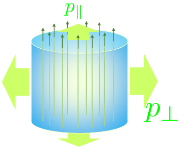
Figure 1: Anisotropic pressure induced by the magnetic field and the magnetization.

We conclude that the leading-order analysis leads to the following constitutive relations

$$T^{\mu\nu}_{(0)} = \epsilon u^{\mu}u^{\nu}-p_{\perp}\Xi^{\mu\nu}+(p_{\perp}-B^{\alpha}H_{\alpha})b^{\mu}b^{\nu}\,,$$ (19a)

$$\tilde{F}^{\mu\nu}_{(0)} = B^{\mu}u^{\nu}-B^{\nu}u^{\mu}\,.$$ (19b)

Note that the derived constitutive relation for $\tilde{F}^{\mu\nu}_{(0)}$ indicates that the electric field is absent at the leading order because it is given by $E^{\mu}_{(0)}:=-\frac{1}{2}\epsilon^{\mu\nu\alpha\beta}u_{\nu}\tilde{F}_{{(0)}\alpha\beta}=0$. This result is consistent with our starting point treating the electric field as a non-hydrodynamic gapped variable. We will find that an electric field (and corresponding electric current) appears as a first-order derivative correction. This will clearly show that they are slaved to the true hydrodynamic variables in the strict hydrodynamic limit as shown below in the form of the first-order constitutive relation.

II.2.3 First-order derivative corrections: Dissipative RMHD

We proceed to the derivation of the first-order corrections $T_{(1)}^{\mu\nu},\,\tilde{F}_{(1)}^{\mu\nu}$. Being equipped with the identified constraints (18), we can simplify the entropy production rate (17) as

$$\partial_{\mu}s^{\mu} = \beta T_{(1)}^{\mu\nu}\partial_{\mu}u_{\nu}+\tilde{F}_{(1)}^{\mu\nu}\partial_{\mu}(\beta H_{\nu})+\partial_{\mu}\big{(}s_{(1)}^{\mu}-\beta u_{\nu}T_{(1)}^{\mu\nu}-\beta H_{\nu}\tilde{F}_{(1)}^{\mu\nu}\big{)}\,,$$ (20)

where we used $T_{(1)}^{\mu\nu}u_{\nu}=0$. Noting that $u_{\nu}$ and $\beta H_{\nu}$ are independent variables, one can ensure the semi-positive entropy production, or the local second law $\partial_{\mu}s^{\mu}\geq 0$, in any hydrodynamic configuration by requiring that

$${\mathcal{R}}_{u} :=\beta T_{(1)}^{\mu\nu}\partial_{\mu}u_{\nu}\geq 0\,,$$ (21a)

$${\mathcal{R}}_{E} :=\tilde{F}_{(1)}^{\mu\nu}\partial_{\mu}(\beta H_{\nu})\geq 0\,,$$ (21b)

$$s_{(1)}^{\mu} =\beta u_{\nu}T_{(1)}^{\mu\nu}+\beta H_{\nu}\tilde{F}_{(1)}^{\mu\nu}\,.$$ (21c)

As we will see, the first two conditions are satisfied by requiring each term to be a semi-positive bilinear form, which determines the first-order constitutive relations. With the resulting constitutive relations, we can also find the derivative corrections to the entropy current from Eq. (21c). Below, we will separately analyze the constitutive relations for $T_{(1)}^{\mu\nu}$ and $\tilde{F}_{(1)}^{\mu\nu}$.

Electric field and resistivities:

Let us first derive the constitutive relation for $\tilde{F}_{(1)}^{\mu\nu}$, focusing on Eq. (21b). To make ${\mathcal{R}}_{E}$ a semi-positive bilinear, we can express $\tilde{F}_{(1)}^{\mu\nu}$ as

$$\tilde{F}_{(1)}^{\mu\nu}=T\rho^{\mu\nu\rho\sigma}\partial_{[\rho}(\beta H_{\sigma]}).$$ (22)

Here, we introduced a rank-four tensor $\rho^{\mu\nu\rho\sigma}$, which will be identified as a resistivity tensor. As we will see, the semi-positivity of ${\mathcal{R}}_{E}$ and the anti-symmetric property in the Lorentz indices restrict possible structures of the resistivity tensor $\rho^{\mu\nu\rho\sigma}$.

To identify the tensor structure of $\rho^{\mu\nu\rho\sigma}$, we first recall that $\tilde{F}_{(1)}^{\mu\nu}$ is transverse to $u^{\nu}$, $\tilde{F}_{(1)}^{\mu\nu}u_{\nu}=0$. Thus, we can use $b^{\mu}$ and $\Xi^{\mu\nu}$ to perform the tensor decomposition of $\rho^{\mu\nu\rho\sigma}$. Moreover, we note that it is anti-symmetric with respect to the exchange of its Lorentz indices $\mu\leftrightarrow\nu$ and $\rho\leftrightarrow\sigma$. Taking into account these properties, we can write down the most general form for $\rho^{\mu\nu\rho\sigma}$ in a neutral plasma as

$$\rho^{\mu\nu\rho\sigma}=2\rho_{\perp}\left(b^{\mu}\Xi^{\nu[\rho}b^{\sigma]}-b^{\nu}\Xi^{\mu[\rho}b^{\sigma]}\right)+2\rho_{\parallel}\Xi^{\mu[\rho}\Xi^{\sigma]\nu}.$$ (23)

The two coefficients $\rho_{\perp,\parallel}$ will be identified with two components of the electric resistivity (see Sec. IV.2). Those tensor structures project out the gradient of the magnetic field in parallel and perpendicular to $b^{\mu}$ as opposed to what the subscripts of $\rho_{\perp,\parallel}$ denote. This is because the electric field is defined with $\widetilde{F}^{\mu\nu}_{(1)}$ and the antisymmetric tensor that swaps the directions (see Eq. (25) below). Note that $\rho^{\mu\nu\rho\sigma}$ cannot have a tensor structure including $b_{\star}^{\mu\nu}:=\varepsilon^{\mu\nu\alpha\beta}u_{\alpha}b_{\beta}$ because any such term would violate the charge-conjugation symmetry. To respect the second law of local thermodynamics, we require semi-positivity of the two resistivities, $\rho_{\parallel}\geq 0$ and $\rho_{\perp}\geq 0$. In fact, substituting Eqs. (22) and (23) into Eq. (21b), we find

$${\mathcal{R}}_{E}=8T\rho_{\perp}\left(b^{[\nu}\Xi^{\mu]\rho}b^{\sigma}\partial_{[\rho}\big{(}\beta H_{\sigma]}\big{)}\right)^{2}+2T\rho_{\parallel}\left(\Xi^{\mu[\rho}\Xi^{\sigma]\nu}\partial_{[\rho}\big{(}\beta H_{\sigma]}\big{)}\right)^{2},$$ (24)

which is positive semi-definite. Equations (22) and (23) complete the constitutive relation for $\tilde{F}_{(1)}^{\mu\nu}$. The first-order corrections to $\tilde{F}_{(1)}^{\mu\nu}$ gives rise to an induced electric field

$$E_{(1)}^{\mu}:=-\frac{1}{2}\varepsilon^{\mu\nu\alpha\beta}u_{\nu}\tilde{F}_{{(1)}\alpha\beta}=(\rho_{\parallel}b^{\mu}b^{\nu}-\rho_{\perp}\Xi^{\mu\nu})T\varepsilon_{\nu\lambda\alpha\beta}u^{\lambda}\partial^{\alpha}(\beta H^{\beta})\,,$$ (25)

where we used an identity $2b_{\star}^{\mu[\alpha}b^{\beta]}=\Xi^{\mu}_{\rho}\epsilon^{\rho\nu\alpha\beta}u_{\nu}$ obtained from the Schouten identity.

Stress tensor and viscosities:

One can derive the first-order corrections to the energy-momentum tensor $T^{\mu\nu}_{(1)}$ in the same manner. To ensure the semi-positivity of (21a), the left-hand side should also be a positive semi-definite bilinear. Introducing the rank-four viscous tensor $\eta^{\mu\nu\rho\sigma}$, we now express $T_{(1)}^{\mu\nu}$ as

$$T_{(1)}^{\mu\nu}=\eta^{\mu\nu\rho\sigma}\partial_{\rho}u_{\sigma},$$ (26)

and identify the tensor structure of $\eta^{\mu\nu\rho\sigma}$.

We first recall that we employ the Landau-Lifshitz frame (see Appendix B for a detailed discussion on the frame choice), in which $T_{(1)}^{\mu\nu}$ is transverse to $u^{\nu}$ as $T_{(1)}^{\mu\nu}u^{\nu}=0$. Thus, we can only use $b^{\mu}$ and $\Xi^{\mu\nu}$ as a possible vector and tensor to decompose the viscous tensor $\eta^{\mu\nu\rho\sigma}$. Note that $b_{\star}^{\mu\nu}$ cannot be used to decompose $\eta^{\mu\nu\rho\sigma}$ because of charge-conjugation symmetry. Moreover, recalling that $T^{\mu\nu}$ is the symmetric energy-momentum tensor, one finds that the viscous tensor should be symmetric with respect to the exchanges between its Lorentz indices $\mu\leftrightarrow\nu$ and $\rho\leftrightarrow\sigma$. These properties allow us to perform the tensor decomposition as

$$\eta^{\mu\nu\rho\sigma}= \zeta_{\parallel}b^{\mu}b^{\nu}b^{\rho}b^{\sigma}+\zeta_{\perp}\Xi^{\mu\nu}\Xi^{\rho\sigma}-\zeta_{\times}(b^{\mu}b^{\nu}\Xi^{\rho\sigma}+\Xi^{\mu\nu}b^{\rho}b^{\sigma})$$

$$-4\eta_{\parallel}b^{(\mu}\Xi^{\nu)(\rho}b^{\sigma)}+\eta_{\perp}\left(\Xi^{\mu\alpha}\Xi^{\nu\beta}+\Xi^{\nu\alpha}\Xi^{\mu\beta}-\Xi^{\mu\nu}\Xi^{\alpha\beta}\right),$$ (27)

where we introduced five viscosities — three bulk viscosities $\zeta_{\parallel},\zeta_{\perp},\zeta_{\times}$ and two shear viscosities $\eta_{\parallel},\eta_{\perp}$. As we will specify, these viscosities must satisfy a semi-positivity constraint to ensure the second law of local thermodynamics.

To get a physical intuition of the dissipative processes and find the semi-positivity constraint attached to each viscosity, it is useful to decompose the velocity gradient as

$$\partial_{(\mu}u_{\nu)}=-\theta_{\parallel}b_{\mu}b_{\nu}+\frac{1}{2}\theta_{\perp}\Xi_{\mu\nu}-2b_{\alpha}b_{(\mu}\Xi_{\nu)\beta}\partial^{(\alpha}u^{\beta)}+\partial_{\{\mu}u_{\nu\}},$$ (28)

where we defined $\theta_{\parallel}:=(-b^{\mu}b^{\nu})\partial_{\mu}u_{\nu}$, $\theta_{\perp}:=\Xi^{\mu\nu}\partial_{\mu}u_{\nu}$, and

$$\partial_{\{\mu}u_{\nu\}}:=\frac{1}{2}\left(\Xi_{\alpha\mu}\Xi_{\nu\beta}+\Xi_{\alpha\nu}\Xi_{\mu\beta}-\Xi_{\mu\nu}\Xi_{\alpha\beta}\right)\partial^{\alpha}u^{\beta}.$$ (29)

Using this decomposition, we find the first-order derivative corrections to the constitutive relation (26) to be

$$T_{(1)}^{\mu\nu}= -(\zeta_{\parallel}\theta_{\parallel}+\zeta_{\times}\theta_{\perp})b^{\mu}b^{\nu}+(\zeta_{\perp}\theta_{\perp}+\zeta_{\times}\theta_{\parallel})\Xi^{\mu\nu}-4\eta_{\parallel}b^{(\mu}\Xi^{\nu)(\rho}b^{\sigma)}\partial_{\rho}u_{\sigma}+2\eta_{\perp}\partial^{\{\mu}u^{\nu\}}.$$ (30)

Equation (30) allows us to get a physical intuition on the dissipative process attached to each viscosity. Without the magnetic flux, an expansion/compression rate is given as $\theta=\nabla_{\mu}u^{\mu}$. In the presence of the magnetic flux,the expansion/compression in the parallel and perpendicular directions should be distinguished from each other, and thus, we have $\theta_{\parallel}$ and $\theta_{\perp}$. Two viscosities $\zeta_{\parallel}$ and $\zeta_{\perp}$ describes a resistance to such two expansion/compression, respectively. Similarly, the flow gradient for the shear deformation is projected into the parallel and perpendicular directions, which leads to the two friction-like processes described by $\eta_{\parallel}$ and $\eta_{\perp}$ (cf. Figs. 2 and 3). Based on these observations, we identify two coefficients $\zeta_{\parallel}$ and $\zeta_{\perp}$ with bulk viscosities and another two coefficients $\eta_{\parallel}$ and $\eta_{\perp}$ with shear viscosities. Besides, there is an off-diagonal cross response proportional to $\zeta_{\times}$. We also identify $\zeta_{\times}$ as one of the bulk viscosities since the associated term describes the cross response of the anisotropic pressures to the two expansion/compression rates (cf. Fig. 4). These processes are reciprocal to one another, and the associated transport coefficients should be the same according to the Onsager’s reciprocal relation Onsager (1931); Hooyman et al. (1954); De Groot and Mazur (1962); Grozdanov et al. (2017). Putting $\zeta_{\parallel}=\zeta_{\perp}=\zeta_{\times}$ and $\eta_{\parallel}=\eta_{\perp}$, one can confirm that the anisotropic viscous corrections in Eq. (30) reduce to the isotropic form (6) by the use of $\theta=\theta_{\parallel}+\theta_{\perp}$ and the identity (28).

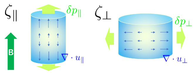
Figure 2: Longitudinal and transverse bulk viscosities that are the off-equilibrium responses of the pressure (green arrows) in the direction of the expansion/compression (blue arrows) of the system.

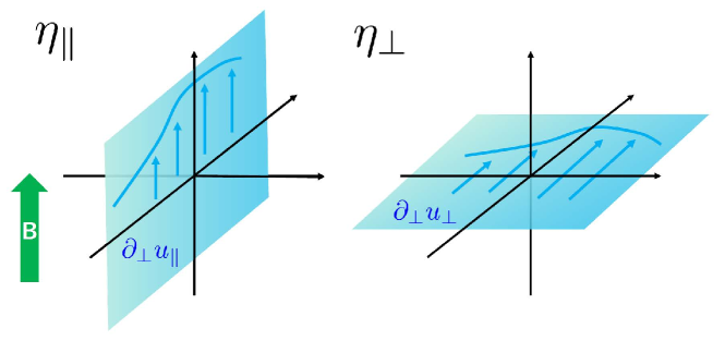
Figure 3: Shear deformations in and out of planes with respect to the magnetic field direction.

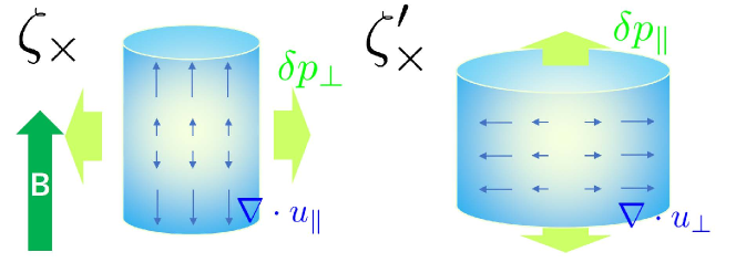
Figure 4: Cross bulk viscosities that are the response of the pressure (green arrows) in the orthogonal direction to the expansion/compression (blue arrows) of the system. Those two cases are reciprocal processes to each other. Compare those two with Fig. 2.

We next investigate the positivity constraint required for the viscosities. Substituting the decomposition (28) into Eq. (21a), we obtain

$${\mathcal{R}}_{u} =\beta\eta^{\mu\nu\rho\sigma}\partial_{\mu}u_{\nu}\partial_{\rho}u_{\sigma}$$

$$=\beta\begin{pmatrix}\theta_{\parallel}&\theta_{\perp}\end{pmatrix}\begin{pmatrix}\zeta_{\parallel}&\zeta_{\times}\\ \zeta_{\times}&\zeta_{\perp}\end{pmatrix}\begin{pmatrix}\theta_{\parallel}\\ \theta_{\perp}\end{pmatrix}+2\beta\eta_{\parallel}\big{(}2b_{(\mu}\Xi_{\nu)\rho}b_{\sigma}\partial^{\rho}u^{\sigma}\big{)}^{2}+2\beta\eta_{\perp}\big{(}\partial_{\{\mu}u_{\nu\}}\big{)}^{2}\,.$$ (31)

Firstly, the last two terms are positive semi-definite by requiring $\eta_{\parallel}\geq 0$ and $\eta_{\perp}\geq 0$. On the other hand, for the first term to respect the local second law, the matrix composed of the bulk viscosities should be positive semi-definite. This means that the eigenvalue of that matrix needs to be non-negative: $\zeta_{\parallel}+\zeta_{\perp}\geq\pm\sqrt{(\zeta_{\parallel}-\zeta_{\perp})^{2}+4\zeta_{\times}^{2}}$. Notice also that the semi-positivity should be separately ensured in a parallel expansion/compression ($\theta_{\parallel}\not=0,\ \theta_{\perp}=0$) and in a perpendicular one ($\theta_{\perp}\not=0,\ \theta_{\parallel}=0$) as necessary conditions, requiring that $\zeta_{\parallel}\geq 0$ and $\zeta_{\perp}\geq 0$. Then, we find an inequality, $\zeta_{\parallel}\zeta_{\perp}-\zeta_{\times}^{2}\geq 0$, from the above eigenvalues. Summarizing, we found five inequalities

$$\eta_{\parallel}\geq 0\,,\ \ \ \eta_{\perp}\geq 0\,,\ \ \ \zeta_{\parallel}\geq 0\,,\ \ \ \zeta_{\perp}\geq 0\,,\ \ \ \zeta_{\parallel}\zeta_{\perp}-\zeta_{\times}^{2}\geq 0\,.$$ (32)

Since the third and fifth (fourth and fifth) inequalities imply the fourth (third) inequality, one can get rid of either third or fourth inequality. See Appendix D for more discussions and comparisons to the results in the literature. We also note that the second law of local thermodynamics does not require the sign of $\zeta_{\times}$ to be semi-positive, but requires an inequality among $\zeta_{\times}$ and $\zeta_{\parallel,\perp}$.

III Nonequilibrium statistical operator method for relativistic MHD

From the underlying quantum field theory, one can also derive RMHD equations by generalizing the nonequilibrium statistical operator method which was initiated by some Japanese physicists in 1950s Nakajima (1957); Mori (1958), further developed in 1960-1970s McLennan (1960, 1988); Kawasaki and Gunton (1973); Zubarev et al. (1979, 1996, 1997), and sophisticated quite recently Sasa (2014); Becattini et al. (2015); Hayata et al. (2015); Hongo (2017, 2019); Becattini et al. (2019); Hongo and Hidaka (2019); Hongo and Hattori (2021). We here review such an approach for deriving RMHD (see Ref. Hongo and Hattori (2021) for more details).

III.1 Optimized perturbation with local Gibbs distribution

The vital point in the nonequilibrium statistical operator method is to correctly identify the appropriate form of the density operator. As we already discussed, the dynamical variables in RMHD are the energy-momentum density $T^{0}_{~{}\mu}$ and the magnetic flux density $\widetilde{F}^{0\mu}$ in a given coordinate system. Let us first identify these operators by considering QED as an underlying quantum theory. The QED Lagrangian is given by

$$\mathcal{L}_{\mathrm{QED}}=\mathrm{i}{\bar{\psi}}\gamma^{\mu}D_{\mu}\psi-m{\bar{\psi}}\psi-\frac{1}{4}\eta^{\mu\nu}\eta^{\alpha\beta}F_{\mu\alpha}F_{\nu\beta},$$ (33)

where we introduced the Dirac field $\psi$ with electric charge $q$, its Dirac conjugate ${\bar{\psi}}=\psi^{\dagger}\gamma^{0}$, and the $\mathrm{U}(1)$ gauge field $A_{\mu}$. We also defined the covariant derivative $D_{\mu}\psi:=\partial_{\mu}\psi-\mathrm{i}qA_{\mu}\psi$ and the field strength tensor $F_{\mu\nu}:=\partial_{\mu}A_{\nu}-\partial_{\nu}A_{\mu}$. The Poincaré symmetry and the Bianchi identity enables us to find that the operators ,

$$\hat{T}^{\mu}_{~{}\nu}=\mathrm{i}{\bar{\psi}}\gamma^{\mu}D_{\nu}\psi+F^{\mu\rho}F_{\nu\rho}-\delta^{\mu}_{\nu}\mathcal{L}_{\mathrm{QED}},\quad\widetilde{F}^{\mu\nu}=\frac{1}{2}\varepsilon^{\mu\nu\rho\sigma}F_{\rho\sigma},$$ (34)

satisfy the following Ward-Takahashi identities:

$$\partial_{\mu}\hat{T}^{\mu}_{~{}\nu}(t,{\bm{x}})=0,\quad\partial_{\mu}\widetilde{F}^{\mu\nu}(t,{\bm{x}})=0.$$ (35)

One may wonder how the Bianchi identity is related to the symmetry of QED. In fact, it is not so obvious how the QED Lagrangian is equipped with the corresponding symmetry — the magnetic $\mathrm{U}(1)$ one-form symmetry — since it does not act on the local operator sitting in Eq. (33). Rather, it acts on the line operator $\displaystyle{\exp\left(\mathrm{i}\int_{C}\mathrm{d}x^{\mu}\widetilde{A}_{\mu}\right)}$, called the t’ Hooft line operator composed of a dual gauge field $\widetilde{A}_{\mu}$ defined by $\widetilde{F}_{\mu\nu}=\partial_{\mu}\widetilde{A}_{\nu}-\partial_{\nu}\widetilde{A}_{\mu}$. The insertion of the t’Hooft line is regarded as putting the test particle with the magnetic charge and is analogous to the insertion of the Wilson line Gaiotto et al. (2015). Thus, considering Eq. (35) as the equations of motion is on the canonical line to set the starting point in constructing a symmetry-based effective theory.

We then identify $T^{\mu\nu}$ and $\widetilde{F}^{\mu\nu}$ in the previous section with expectation values of the above quantum operators $\hat{T}^{\mu\nu}$ and $\widetilde{F}^{\mu\nu}$. This identification motivates us to specify the appropriate density operator as the one describing fixed expectation values of our dynamical variables $\langle\hat{T}^{0}_{~{}\nu}(t,{\bm{x}})\rangle$ and $\langle\widetilde{F}^{0\mu}(t,{\bm{x}})\rangle$. The so-called local Gibbs (LG) distribution $\hat{\rho}_{\mathrm{LG}}[\lambda_{t};t]$ realizes such an density operator, which is parameterized by a set of the Lagrange multipliers $\lambda_{t}:=\{\beta^{\mu}(t,{\bm{x}}),\mathcal{H}_{\nu}(t,{\bm{x}})\}$ as

$$\hat{\rho}_{\mathrm{LG}}[\lambda_{t};t]:=\exp(-\hat{S}[\lambda_{t};t]),$$ (36)

where we introduced the entropy functional operator

$$\hat{S}[\lambda_{t};t]:=-\int\mathrm{d}^{3}x\left[\hat{T}^{0}_{~{}\nu}(t,{\bm{x}})\beta^{\nu}(t,{\bm{x}})+\widetilde{F}^{0\nu}(t,{\bm{x}})\mathcal{H}_{\nu}(t,{\bm{x}})\right]+\Psi[\lambda_{t}].$$ (37)

Here, the first argument $\lambda_{t}$ in $\hat{\rho}_{\mathrm{LG}}[\lambda_{t};t]$ and $\hat{S}[\lambda_{t};t]$ describes their functional dependence on the Lagrange multipliers, $\lambda_{t}:=\{\beta^{\mu}(t,{\bm{x}}),\mathcal{H}_{\nu}(t,{\bm{x}})\}$, while the second one $t$ represents the time argument for a set of the conserved charge-density operators $\hat{c}_{t}:=\{\hat{T}^{0}_{~{}\nu}(t,{\bm{x}}),\widetilde{F}^{0\mu}(t,{\bm{x}})\}$. One finds that these Lagrange multipliers can be decomposed as $\beta^{\mu}(t,{\bm{x}})=\beta(t,{\bm{x}})u^{\mu}(t,{\bm{x}})$ and $\mathcal{H}_{\mu}(t,{\bm{x}})=\beta(t,{\bm{x}})H_{\mu}(t,{\bm{x}})$ with the local inverse temperature $\beta(t,{\bm{x}})$, the fluid four-velocity $u^{\mu}(t,{\bm{x}})$, and the magnetic field $H_{\mu}(t,{\bm{x}})$. In the following, we express the average of a quantum operator $\hat{\mathcal{O}}$ over the LG distribution as

$$\langle\hat{\mathcal{O}}\rangle^{\text{LG}}_{\lambda_{t}}:={\rm Tr}(\hat{\rho}_{\mathrm{LG}}[\lambda_{t};t]\hat{\mathcal{O}}).$$ (38)

In Eq. (37), we also defined the local thermodynamic functional $\Psi[\lambda_{t}]$, called the Massieu-Planck functional, as a normalization factor of the LG distribution

$$\Psi[\lambda_{t}]:=\log{\rm Tr}\exp\left(\int\mathrm{d}^{3}x\left[\hat{T}^{0}_{~{}\mu}(t,{\bm{x}})\beta^{\mu}(t,{\bm{x}})+\widetilde{F}^{0\mu}(t,{\bm{x}})\mathcal{H}_{\mu}(t,{\bm{x}})\right]\right).$$ (39)

This functional is used to extract the average charge densities

$$\langle\hat{T}^{0}_{~{}\mu}(t,{\bm{x}})\rangle^{\text{LG}}=\frac{\delta\Psi[\lambda_{t}]}{\delta\beta^{\mu}(t,{\bm{x}})},\quad\langle\widetilde{F}^{0\mu}(t,{\bm{x}})\rangle^{\text{LG}}=\frac{\delta\Psi[\lambda_{t}]}{\delta\mathcal{H}_{\mu}(t,{\bm{x}})}.$$ (40)

Besides, we define the entropy functional $S[c_{t}]$ by taking the average of Eq. (37) over $\hat{\rho}_{\mathrm{LG}}[\lambda_{t};t]$ as

$$S[c_{t}]:=-\int\mathrm{d}^{3}x\left[\langle\hat{T}^{0}_{~{}\nu}(t,{\bm{x}})\rangle^{\text{LG}}_{\lambda_{t}}\beta^{\nu}(t,{\bm{x}})+\langle\widetilde{F}^{0\nu}(t,{\bm{x}})\rangle^{\text{LG}}_{\lambda_{t}}\mathcal{H}_{\nu}(t,{\bm{x}})\right]+\Psi[\lambda_{t}].$$ (41)

In other words, the entropy functional $S[c_{t}]$ is defined by the Legendre transform of the Massieu-Planck functional $\Psi[\lambda_{t}]$, and thus, its argument is the averaged charge densities $c_{t}=\{\langle\hat{T}^{0}_{~{}\nu}(t,{\bm{x}})\rangle^{\text{LG}}_{\lambda_{t}},\langle\widetilde{F}^{0\mu}(t,{\bm{x}})\rangle^{\text{LG}}_{\lambda_{t}}\}$. One then finds that the Lagrange multipliers, or local thermodynamic variables conjugate to the conserved charge densities, as

$$\beta^{\mu}(t,{\bm{x}})=-\frac{\delta S[c_{t}]}{\delta T^{0}_{~{}\mu}(t,{\bm{x}})},\quad\mathcal{H}_{\mu}(t,{\bm{x}})=-\frac{\delta S[c_{t}]}{\delta\widetilde{F}^{0\mu}(t,{\bm{x}})},$$ (42)

which are consistent with Eq. (14) in the previous section.

To describe the dissipative transport phenomena with the nonequilibrium statistical operator method, we require a crucial assumption that the density operator $\hat{\rho}_{0}$ at the initial time $t_{0}$ be given by the LG distribution $\hat{\rho}_{0}=\hat{\rho}_{\mathrm{LG}}[\lambda_{t_{0}};t_{0}]$ Zubarev et al. (1979, 1996, 1997); Sasa (2014); Hayata et al. (2015); Hongo and Hattori (2021). Using the Heisenberg picture, we define the expectation value of an arbitrary Heisenberg operator $\hat{\mathcal{O}}(t)$ at time $t(\geq t_{0})$ as

$$\langle\hat{\mathcal{O}}(t)\rangle:={\rm Tr}[\hat{\rho}_{0}\hat{\mathcal{O}}(t)]=\langle\hat{\mathcal{O}}(t)\rangle^{\text{LG}}_{\lambda_{t_{0}}},$$ (43)

where we expressed the rightmost side using the above assumption and Eq. (38). Then, according to our identification, the averaged Ward-Takahashi identities,

$$\partial_{\mu}\langle\hat{T}^{\mu}_{~{}\nu}(t,{\bm{x}})\rangle=0,\quad\partial_{\mu}\langle\widetilde{F}^{\mu\nu}(t,{\bm{x}})\rangle=0,$$ (44)

should provide the RMHD equations after an appropriate derivative expansion is employed.

From this microscopic point of view, we have already fixed the definition of expectation values $\langle\hat{T}^{\mu}_{~{}\nu}(t,{\bm{x}})\rangle$ and $\langle\widetilde{F}^{\mu\nu}(t,{\bm{x}})\rangle$ by Eq. (43). Thus, the remaining problem is to derive the constitutive relations for Eq. (43) based on our density operator $\hat{\rho}_{0}=\hat{\rho}_{\mathrm{LG}}[\lambda_{t_{0}};t_{0}]$. However, recalling the result in the previous section, one realizes that this is a tough problem; We expect that the resulting constitutive relations should be expressed by the conjugate variables $\lambda_{t}$ at time $t$, whereas our density operator $\hat{\rho}_{0}=\hat{\rho}_{\mathrm{LG}}[\lambda_{t_{0}};t_{0}]$ only contains those $\lambda_{t_{0}}$ at the initial time $t_{0}$. In fact, the expectation value at time $t\,(>t_{0})$ in the present setup is always defined by taking average over the initial density operator $\hat{\rho}_{0}=\hat{\rho}_{\mathrm{LG}}[\lambda_{t_{0}};t_{0}]$, which only contains conjugate variables at the initial time. Thus, it sounds impossible to express $\langle\hat{T}^{\mu}_{~{}\nu}(t,{\bm{x}})\rangle$ and $\langle\widetilde{F}^{\mu\nu}(t,{\bm{x}})\rangle$ in terms of $\lambda_{t}$ at time $t$ as we did in the previous section.

The above observation implies that the initial density operator $\hat{\rho}_{0}=\hat{\rho}_{\mathrm{LG}}[\lambda_{t_{0}};t_{0}]$ does not give a useful starting point to evaluate the expectation value at later time $t(>t_{0})$. Instead, one immediately finds that the better starting point is the local Gibbs distribution at time $t$. The question is how we can shift into such a different distribution when we do not even have conjugate variables other than those at initial time $t_{0}$.

We can resolve this problem by invoking the optimized (or renormalized) perturbation theory (see, e.g., Refs. Stevenson (1981); Kleinert (2009); Jakovác and Patkós (2015)). Suppose that we know the configuration of the conserved charge densities at time $t$. With the help of the entropy functional $S[c_{t}]$, we first define the conjugate variable $\lambda_{t}$ by Eq. (42). One can show that this definition is equivalent to requiring the following matching conditions

$$\langle T^{0}_{~{}\nu}\rangle=\langle T^{0}_{~{}\nu}\rangle^{\text{LG}}_{\lambda_{t}},\quad\langle\widetilde{F}^{0\nu}\rangle=\langle\widetilde{F}^{0\nu}\rangle^{\text{LG}}_{\lambda_{t}}.$$ (45)

Using the defined conjugate variables $\lambda_{t}$, we rearrange our density operator as

$$\hat{\rho}_{0}=\mathrm{e}^{-\hat{S}[\lambda_{t};t]+\hat{\Sigma}[t,t_{0};\lambda]}=\mathrm{e}^{-\hat{S}[\lambda_{t};t]}\mathrm{T}_{\tau}\exp\left(\int_{0}^{1}\mathrm{d}\tau\mathrm{e}^{\tau\hat{S}[\lambda_{t};t]}\hat{\Sigma}[t,t_{0};\lambda]\mathrm{e}^{-\tau\hat{S}[\lambda_{t};t]}\right),$$ (46)

where we just added and subtracted the entropy operator $\hat{S}[t;\lambda_{t}]$ at time $t$ and defined the entropy production operator $\hat{\Sigma}[t,t_{0};\lambda]$ as

$$\hat{\Sigma}[t,t_{0};\lambda]:=\hat{S}[\lambda_{t};t]-\hat{S}[\lambda_{t_{0}};t_{0}].$$ (47)

The rightmost side of Eq. (46) gives a useful formula for the derivative expansion since the entropy production operator $\hat{\Sigma}[t,t_{0};\lambda]$ will be shown to be $O(\partial^{1})$. Thus, we can regard $\hat{\Sigma}[t,t_{0};\lambda]$ as a derivative correction, and Eq. (46) gives a familiar perturbative expansion formula in the interacting picture, which we learn in the elementary course of quantum mechanics. As a result, we see that the nonequilibrium statistical operator method gives one useful expansion scheme relying on the new optimized (or renormalized) parameter $\lambda_{t}$.

Expanding the rightmost side of Eq. (46) at the first-order in $\hat{\Sigma}[t,t_{0};\lambda]$, we obtain

$$\begin{split}\langle\hat{T}^{\mu\nu}(t,{\bm{x}})\rangle&=\langle\hat{T}^{\mu\nu}(t,{\bm{x}})\rangle^{\text{LG}}_{\lambda_{t}}+\bm{(}{\hat{T}^{\mu\nu}(t,{\bm{x}}),\hat{\Sigma}[t,t_{0};\lambda]}\bm{)}_{t}+O(\hat{\Sigma}^{2}),\\ \langle\widetilde{F}^{\mu\nu}(t,{\bm{x}})\rangle&=\langle\widetilde{F}^{\mu\nu}(t,{\bm{x}})\rangle^{\text{LG}}_{\lambda_{t}}+\bm{(}{\widetilde{F}^{\mu\nu}(t,{\bm{x}}),\hat{\Sigma}[t,t_{0};\lambda]}\bm{)}_{t}+O(\hat{\Sigma}^{2}),\end{split}$$ (48)

where we introduced the Kubo-Mori-Bogoliubov inner product:

$$\bm{(}{\hat{A},\hat{B}}\bm{)}_{t}:=\int_{0}^{1}\mathrm{d}\tau\langle\mathrm{e}^{\tau\hat{S}[\lambda_{t};t]}\hat{A}\mathrm{e}^{-\tau\hat{S}[\lambda_{t};t]}\hat{B}^{{\dagger}}\rangle^{\text{LG}}_{\lambda_{t}}.$$ (49)

Equation (48) indicates that we have separated the problem into two parts: The first one is to evaluate the expectation value of currents with the LG distribution describing the local thermal equilibrium

$$T^{\mu\nu}_{(0)}=\langle\hat{T}^{\mu\nu}(t,{\bm{x}})\rangle^{\text{LG}}_{\lambda_{t}},\quad\widetilde{F}^{\mu\nu}_{(0)}=\langle\widetilde{F}^{\mu\nu}(t,{\bm{x}})\rangle^{\text{LG}}_{\lambda_{t}},$$ (50)

which will be shown to contain the leading-order terms in derivative. The second one is to find the dissipative corrections

$$T^{\mu\nu}_{(1)}=\bm{(}{\hat{T}^{\mu\nu}(t,{\bm{x}}),\hat{\Sigma}[t,t_{0};\lambda]}\bm{)}_{t},\quad\widetilde{F}^{\mu\nu}_{(1)}=\bm{(}{\widetilde{F}^{\mu\nu}(t,{\bm{x}}),\hat{\Sigma}[t,t_{0};\lambda]}\bm{)}_{t},$$ (51)

by computing the entropy production.

III.2 Evaluating the Local Gibbs averages

Let us first investigate the LG-averaged currents given in Eq. (50). In evaluating these expectation values, it is useful to put our system in the curved spacetime described by the vierbein $e_{\mu}^{~{}a}$ and introduce a background two-form gauge field $b_{\mu\nu}$ that couples to $\widetilde{F}^{\mu\nu}$. In the presence of these background fields, one can show the following variational formulas Hongo and Hattori (2021)

$$\begin{split}\langle\hat{T}^{\mu\nu}(t,{\bm{x}})\rangle^{\text{LG}}_{\lambda_{t}}&=\frac{1}{\beta^{0}\sqrt{\gamma}}\frac{\delta\Psi[\lambda_{t}]}{\delta e_{\mu}^{~{}a}(t,{\bm{x}})}e^{\nu}_{~{}a},\\ \langle\widetilde{F}^{\mu\nu}(t,{\bm{x}})\rangle^{\text{LG}}_{\lambda_{t}}&=\frac{2}{\beta^{0}\sqrt{\gamma}}\left(\beta^{[\mu}\delta^{\nu]}_{\rho}\frac{\delta\Psi[\lambda_{t}]}{\delta\mathcal{H}_{\rho}(t,{\bm{x}})}+\frac{\delta\Psi[\lambda_{t}]}{\delta b_{\mu\nu}(t,{\bm{x}})}\right),\end{split}$$ (52)

where $e^{\nu}_{~{}a}$ is the inverse of vierbein and $\beta^{0}$ denotes the zeroth-component of the four vector $\beta^{\mu}$. Here, we also used $\gamma:=\det g_{ij}$ with a spatial part of the metric $g_{ij}=e_{i}^{~{}a}e_{j}^{~{}b}\eta_{ab}$. Thus, we can derive the LG expectation values $\langle\hat{T}^{\mu\nu}(t,{\bm{x}})\rangle^{\text{LG}}_{\lambda_{t}}$ and $\langle\widetilde{F}^{\mu\nu}(t,{\bm{x}})\rangle^{\text{LG}}_{\lambda_{t}}$ once we get the form of the local thermodynamic functional $\Psi[\lambda_{t}]$ under the background fields.

To specify the form of the Massieu-Planck functional $\Psi[\lambda_{t}]$, we can rely on the path-integral formula Hongo (2017); Hongo and Hattori (2021). Substituting Eq. (34) into the definition (39) of $\Psi[\lambda_{t}]$ and following the usual procedure of deriving the path-integral representation for the partition function, we obtain

$$\Psi[\lambda_{t}]=\log\int\mathcal{D}\psi\mathcal{D}{\bar{\psi}}\mathcal{D}A_{\mu}\delta(F)\det(\partial F/\partial\alpha)\exp\left(\int_{0}^{\beta_{\mathrm{ref}}}\mathrm{d}\tau\mathrm{d}^{3}x\sqrt{-\tilde{g}}\widetilde{\mathcal{L}}_{\mathrm{QED}}\right),$$ (53)

where $\beta_{\mathrm{ref}}$ is an arbitrary constant reference inverse temperature and $F$ denotes a gauge fixing condition $F=0$ with a gauge parameter $\alpha$. Due to the inhomogeneity of the local thermodynamic variables $\lambda_{t}$, we need to perform the path-integral not in the flat Euclidean spacetime but in the emergent curved spacetime with the two-form gauge field. In fact, we find the Lagrangian density in Eq. (53) to be

$$\widetilde{\mathcal{L}}_{\mathrm{QED}}=\mathrm{i}{\bar{\psi}}\gamma^{a}\tilde{e}_{a}^{~{}\mu}\widetilde{D}_{\mu}\psi-m{\bar{\psi}}\psi-\frac{1}{4}\tilde{g}^{\mu\nu}\tilde{g}^{\alpha\beta}F_{\mu\alpha}F_{\nu\beta}+\frac{1}{2}\tilde{b}_{\mu\nu}\widetilde{F}^{\mu\nu},$$ (54)

and the background fields — the thermal vierbein $\tilde{e}_{\mu}^{~{}a}$ and thermal two-form gauge field $\tilde{b}_{\mu\nu}$ — are given by

$$\tilde{e}_{0}^{~{}a}:=\mathrm{e}^{\sigma}u^{a},\quad\tilde{e}_{i}^{~{}a}:=e_{i}^{~{}a},\quad\tilde{b}_{0i}:=\mathrm{e}^{\sigma}H_{i},\quad\tilde{b}_{ij}:=b_{ij},$$ (55)

where we defined $\mathrm{e}^{\sigma(x)}=\beta(x)/\beta_{\mathrm{ref}}$. We also defined the thermal metric $\tilde{g}_{\mu\nu}:=\tilde{e}_{\mu}^{~{}a}\tilde{e}_{\nu}^{~{}b}\eta_{ab}$ with $\tilde{g}:=\det\tilde{g}_{\mu\nu}$, and the covariant derivative

$$\widetilde{D}_{\mu}\psi:=\tilde{\partial}_{\mu}\psi-\mathrm{i}qA_{\mu}\psi-\frac{\mathrm{i}}{2}\widetilde{\omega}_{\mu}^{~{}ab}\Sigma_{ab}\psi,$$ (56)

with the representation matrix of the Dirac spinor under the Lorentz transformation $\Sigma_{ab}:=\mathrm{i}[\gamma_{a},\gamma_{b}]/4$. The derivative in the thermal space is given as $\tilde{\partial}_{\mu}=(\mathrm{i}\partial_{\tau},\partial_{i})$ and the spin connection $\widetilde{\omega}_{\mu}^{~{}ab}$ is determined by the thermal vierbein $\tilde{e}_{\mu}^{~{}a}$ as Hongo (2017)

$$\widetilde{\omega}_{\mu}^{~{}ab}=\frac{1}{2}\tilde{e}^{a\nu}\tilde{e}^{b\rho}(\widetilde{C}_{\nu\rho\mu}-\widetilde{C}_{\rho\nu\mu}-\widetilde{C}_{\mu\nu\rho})\quad{\rm with}\quad\widetilde{C}_{\mu\nu\rho}:=\tilde{e}_{\mu}^{~{}c}\big{(}\tilde{\partial}_{\nu}\tilde{e}_{\rho c}-\tilde{\partial}_{\rho}\tilde{e}_{\nu c}\big{)}.$$ (57)

In short, the Massieu-Planck functional is described by performing the path integral for QED in the presence of the curved and two-form backgrounds. This result is a generalization of the background field method to the locally thermalized system. We can read off the symmetry properties of the Massieu-Planck functional as follows. To see this, note that the line element $\mathrm{d}\tilde{s}^{2}$ and two-form gauge connection $\tilde{b}$,

$$\mathrm{d}\tilde{s}^{2} :=\tilde{g}_{\mu\nu}\mathrm{d}\tilde{x}^{\mu}\otimes\mathrm{d}\tilde{x}^{\nu}=-\mathrm{e}^{2\sigma}(\mathrm{d}\tilde{t}+a_{i}\mathrm{d}x^{i})^{2}+g^{\prime}_{ij}\mathrm{d}x^{i}\otimes\mathrm{d}x^{j},$$ (58)

$$\tilde{b} :=\frac{1}{2}\tilde{b}_{\mu\nu}\mathrm{d}\tilde{x}^{\mu}\wedge\mathrm{d}\tilde{x}^{\nu}=\tilde{b}_{0i}(\mathrm{d}\tilde{t}+a_{j}\mathrm{d}x^{j})\wedge\mathrm{d}x^{i}+\frac{1}{2}\tilde{b}_{ij}^{\prime}\mathrm{d}x^{i}\wedge\mathrm{d}x^{j},$$ (59)

describe the backgrounds. Here, we defined $(\mathrm{d}\tilde{t},\mathrm{d}\widetilde{\bm{x}})=(-\mathrm{i}\mathrm{d}\tau,\mathrm{d}{\bm{x}})$ and expressed $\mathrm{d}\tilde{s}^{2}$ and $\tilde{b}$ using the Kaluza-Klein parameterization

$$a_{i}:=-\mathrm{e}^{-\sigma}u_{i},\quad g^{\prime}_{ij}:=g_{ij}+u_{i}u_{j},\quad\tilde{b}_{ij}^{\prime}:=b_{ij}-\tilde{b}_{0j}a_{i}-\tilde{b}_{i0}a_{j}.$$ (60)

The apparently complicated Kaluza-Klein parameterization is, indeed, useful because the Massieu-Planck functional is invariant under the Kaluza-Klein gauge transformation

$$\begin{split}\tilde{t}&\to\tilde{t}^{\prime}=\tilde{t}+\chi({\bm{x}}),\\ {\bm{x}}&\to{\bm{x}}^{\prime}={\bm{x}},\\ a_{i}({\bm{x}})&\to a_{i}^{\prime}({\bm{x}})=a_{i}({\bm{x}})-\partial_{i}\chi({\bm{x}}),\end{split}$$ (61)

and $\mathrm{e}^{\sigma}$, $\gamma_{ij}^{\prime}$ and $\tilde{b}_{0i}$ and $\tilde{b}_{ij}^{\prime}$ are all invariant under the Kaluza-Klein gauge transformation. Besides, the Massieu-Planck functional is invariant under the spatial diffeomorphism and gauge transformation acting on $b_{ij}$,

$$x^{i} \to x^{i\prime}=f^{i}({\bm{x}}),$$ (62)

$$\tilde{b}_{ij} \to\tilde{b}_{ij}+\partial_{i}\theta_{j}-\partial_{j}\theta_{i}.$$ (63)

The crucial point here is that the Massieu-Planck functional has to respect the symmetries under the transformations (61)-(63). Using this symmetry property and relying on the derivative expansion, one can write down the most general form of the Massieu-Planck functional in an order-by-order basis in derivative. In the leading-order expansion, we have two zeroth-order invariant scalars $\mathrm{e}^{\sigma(x)}=\beta(x)/\beta_{\mathrm{ref}}$ and $\sqrt{\big{(}\tilde{b}_{0i}(x)\big{)}^{2}}=\mathrm{e}^{\sigma(x)}H(x)=\mathcal{H}(x)/\beta_{\mathrm{ref}}$, where we decomposed the magnetic field as $H_{\mu}=-Hb_{\mu}$ and $\mathcal{H}_{\mu}=-\mathcal{H}b_{\mu}$ with the normalized spatial vector $b^{\mu}$. Moreover, there is no invariant scalar at $O(\partial^{1})$, and thus, the most general form of $\Psi[\lambda]$ in the leading-order expansion is given by

$$\begin{split}\Psi[\lambda]&=\int_{0}^{\beta_{\mathrm{ref}}}\mathrm{d}\tau\mathrm{d}^{3}x\sqrt{-\tilde{g}}p(\beta,\mathcal{H})+O(\partial^{2})=\int\mathrm{d}^{3}x\sqrt{\gamma}\beta^{0}p(\beta,\mathcal{H})+O(\partial^{2}).\end{split}$$ (64)

Recalling the variational formula (52), we find that the functional derivative of Eq. (64) leads to

$$\begin{split}\langle\hat{T}^{\mu\nu}(t,{\bm{x}})\rangle^{\text{LG}}_{\lambda_{t}}&=\epsilon u^{\mu}u^{\nu}-p_{\perp}(\eta^{\mu\nu}-u^{\mu}u^{\nu}+b^{\mu}b^{\nu})+p_{\parallel}b^{\mu}b^{\nu},\\ \langle\widetilde{F}^{\mu\nu}(t,{\bm{x}})\rangle^{\text{LG}}_{\lambda_{t}}&=B(b^{\mu}u^{\nu}-b^{\nu}u^{\mu}),\end{split}$$ (65)

where we have taken the flat background limit and introduced a set of the scalar functions

$$\epsilon=-\frac{\partial(\beta p)}{\partial\beta},\quad p_{\perp}=p,\quad p_{\parallel}=p-\beta^{-1}\mathcal{H}B,\quad B=\beta\frac{\partial p}{\partial\mathcal{H}}.$$ (66)

All of them can be extracted from the single function $p(\beta,\mathcal{H})$. Equations (65)-(66) give the leading-order constitutive relations of RMHD, which agree with Eq. (19) in the previous section (recall $\beta^{-1}\mathcal{H}B=H^{\mu}B_{\mu}$). In contrast to the entropy-current analysis, we now have the microscopic path-integral formula for $p(\beta,\mathcal{H})$. One can thus, in principle, compute all coefficient functions in Eq. (66), or the equations of state, from the underlying microscopic theory, i.e., QED.

III.3 Evaluating the dissipative corrections

We next evaluate the dissipative corrections given in Eq. (51). For this purpose, we first rewrite the entropy production operator by using the Ward-Takahshi identity (35) and performing integration by parts. The resultant expression reads

$$\hat{\Sigma}[t,t_{0};\lambda] :=\hat{S}[\lambda_{t};t]-\hat{S}[\lambda_{t_{0}};t_{0}]=\int_{t_{0}}^{t}\mathrm{d}t^{\prime}\partial_{t^{\prime}}\hat{S}[\lambda_{t^{\prime}};t^{\prime}]$$

$$=-\int_{t_{0}}^{t}\mathrm{d}t^{\prime}\partial_{t^{\prime}}\left[\int\mathrm{d}^{3}x^{\prime}\left(\beta^{\nu}(t^{\prime},{\bm{x}}^{\prime})\hat{T}^{0}_{~{}\nu}(t^{\prime},{\bm{x}}^{\prime})+\mathcal{H}_{\nu}(t^{\prime},{\bm{x}}^{\prime})\widetilde{F}^{0\nu}(t^{\prime},{\bm{x}}^{\prime})\right)+\Psi[\lambda_{t^{\prime}}]\right]$$

$$=-\int_{t_{0}}^{t}\mathrm{d}t^{\prime}\mathrm{d}^{3}x^{\prime}\left[\delta\hat{T}^{\mu\nu}(t^{\prime},{\bm{x}}^{\prime})\partial_{\mu}\beta_{\nu}(t^{\prime},{\bm{x}}^{\prime})+\delta\widetilde{F}^{\mu\nu}(t^{\prime},{\bm{x}}^{\prime})\partial_{\mu}\mathcal{H}_{\nu}(t^{\prime},{\bm{x}}^{\prime})\right],$$ (67)

where we defined a deviation $\delta\hat{\mathcal{O}}(t):=\hat{\mathcal{O}}(t)-\langle\hat{\mathcal{O}}(t)\rangle^{\text{LG}}_{\lambda_{t}}$. To obtain the third line, we also used the following identity:

$$\begin{split}\partial_{t}\Psi[\lambda_{t}]&=-\Big{\langle}\partial_{t}\int\mathrm{d}^{3}x\left(\beta^{\nu}\hat{T}^{0}_{~{}\nu}+\mathcal{H}_{\nu}\widetilde{F}^{0\nu}\right)\Big{\rangle}^{\mathrm{LG}}_{\lambda_{t}}\\ &=\int\mathrm{d}^{3}x\left(\langle\hat{T}^{\mu\nu}\rangle^{\text{LG}}_{\lambda_{t}}\partial_{\mu}\beta_{\nu}+\langle\widetilde{F}^{\mu\nu}\rangle^{\text{LG}}_{\lambda_{t}}\partial_{\mu}\mathcal{H}_{\nu}\right).\end{split}$$ (68)

Note that the entropy production operator $\hat{\Sigma}[t,t_{0};\lambda]$ in Eq. (67) contains the time derivative of the parameters $\lambda_{t^{\prime}}$. This can be explicitly seen by using the projection tensor, $\delta^{\mu}_{\nu}=u^{\mu}u_{\nu}+\Delta^{\mu}_{\nu}$, that decomposes a derivative as

$$\partial_{\mu}=u_{\mu}D+\nabla_{\mu}\quad{\rm with}\quad D:=u^{\mu}\partial_{\mu},\quad\nabla_{\mu}:=\Delta^{\nu}_{\mu}\partial_{\nu}.$$ (69)

Substituting this decomposition together with $\beta^{\mu}=\beta u^{\mu}$ and $\mathcal{H}_{\nu}=-\mathcal{H}b_{\nu}$, we obtain the following expression for the entropy production operator

$$\begin{split}\hat{\Sigma}[t,t_{0};\lambda]=-\int_{t_{0}}^{t}\mathrm{d}t^{\prime}\mathrm{d}^{3}x^{\prime}&\Big{[}u_{\mu}u_{\nu}\delta\hat{T}^{\mu\nu}D\beta+u_{\mu}\delta\hat{T}^{\mu\nu}\beta Du_{\nu}-u_{\mu}b_{\nu}\delta\widetilde{F}^{\mu\nu}D\mathcal{H}-\mathcal{H}u_{\mu}\delta\widetilde{F}^{\mu\nu}Db_{\nu}\\ &+\beta\delta\hat{T}^{\mu\nu}\nabla_{\mu}u_{\nu}+u_{\nu}\delta\hat{T}^{\mu\nu}\nabla_{\mu}\beta+\mathcal{H}\delta\widetilde{F}^{\mu\nu}b^{\rho}u_{\nu}\nabla_{\mu}u_{\rho}+\delta\widetilde{F}^{\mu\nu}\Delta_{\nu}^{\rho}\nabla_{\mu}\mathcal{H}_{\rho}\Big{]}.\end{split}$$ (70)

Here, it is important to eliminate time-derivative terms in the first line. Otherwise, the resulting Green-Kubo formulas pick up contributions from gapless linear hydrodynamic modes, which prevents us from obtaining convergent time integrals for the transport coefficients. In Ref. Hongo and Hattori (2021), we accomplish such a procedure by a formal manipulation. To complement that formal manipulation, we will here explicitly demonstrate this procedure.

To eliminate the time-derivative terms, we solve the leading-order RMHD equations following the leading-order constitutive relations (65). Using Eq. (65), we find the leading-order equations of motion

$$0 =\partial_{\mu}T^{\mu\nu}_{(0)}=\partial_{\mu}\big{[}\epsilon u^{\mu}u^{\nu}-p_{\perp}(\eta^{\mu\nu}-u^{\mu}u^{\nu})+B^{\mu}H^{\nu}\big{]},$$ (71a)

$$0 =\partial_{\mu}\widetilde{F}^{\mu\nu}_{(0)}=\partial_{\mu}[B^{\mu}u^{\nu}-B^{\nu}u^{\mu}],$$ (71b)

where we used $p_{\parallel}=p_{\perp}-HB$ to express $p_{\parallel}$ in terms of $B^{\mu}=Bb^{\nu}$ and $H^{\nu}=-Hb^{\nu}$. After contracting these ideal RMHD equations with appropriate tensors such as $b_{\mu}$, we obtain the following set of equations:

$$D\epsilon =-(\epsilon+p_{\perp})\theta+HB\theta_{\parallel},$$ (72a)

$$(\epsilon+p_{\perp})Du_{\nu} =\nabla_{\nu}p_{\perp}-H_{\nu}\partial_{\mu}B^{\mu}-\Delta_{\nu\rho}B^{\mu}\partial_{\mu}H^{\rho},$$ (72b)

$$DB =-B\theta_{\perp},$$ (72c)

$$Db^{\nu} =\Xi^{\nu\rho}b^{\mu}\partial_{\mu}u_{\rho}+B^{-1}u^{\nu}\partial_{\mu}B^{\mu},$$ (72d)

where we used $\theta=\theta_{\parallel}+\theta_{\perp}$ with $\theta_{\parallel}=-b^{\mu}b^{\nu}\partial_{\mu}u_{\nu}$ and $\theta_{\perp}=\Xi^{\mu\nu}\partial_{\mu}u_{\nu}$. Combining these equations with thermodynamic relations, we can further simplify $Du_{\nu}$ and also find the time derivatives of conjugate variables $D\beta$ and $D\mathcal{H}$ as (see Appendix C for a derivation)

$$D\beta =\beta\left(\frac{\partial p_{\perp}}{\partial\epsilon}-B\frac{\partial H}{\partial\epsilon}\right)\theta_{\parallel}+\beta\frac{\partial p_{\perp}}{\partial\epsilon}\theta_{\perp},$$ (73a)

$$D\mathcal{H} =-\beta\frac{\partial p_{\perp}}{\partial B}\theta_{\perp}-\beta\left(\frac{\partial p_{\perp}}{\partial B}-B\frac{\partial H}{\partial B}\right)\theta_{\parallel},$$ (73b)

$$Du_{\nu} =-\beta^{-1}\nabla_{\nu}\beta-\frac{1}{\epsilon+p_{\perp}}\left[2\beta^{-1}Bb^{\mu}\nabla_{[\mu}\mathcal{H}_{\nu]}+\theta_{\parallel}HBu_{\nu}\right],$$ (73c)

$$Db_{\nu} =\Xi_{\nu}^{~{}\rho}b^{\mu}\nabla_{\mu}u_{\rho}+B^{-1}u_{\nu}\partial_{\mu}B^{\mu}.$$ (73d)

These leading-order equations of motion for thermodynamic parameters enable us to eliminate the time-derivative terms in the entropy production operator. Substituting them into Eq. (70) and rearranging terms, we eventually obtain the entropy production operator

$$\begin{split}\hat{\Sigma}[t,t_{0};\lambda]=-\int_{t_{0}}^{t}\mathrm{d}t^{\prime}\mathrm{d}^{3}x&\Big{[}\tilde{\delta}\hat{p}_{\parallel}\beta\theta_{\parallel}+\tilde{\delta}\hat{p}_{\perp}\beta\theta_{\perp}+2\tilde{\delta}\hat{\pi}^{(\mu}b^{\nu)}\beta\nabla_{\mu}u_{\nu}+\tilde{\delta}\hat{\tau}^{\mu\nu}\beta\nabla_{\mu}u_{\nu}\\ &+2\tilde{\delta}\hat{E}^{[\mu}b^{\nu]}\nabla_{\mu}\mathcal{H}_{\nu}+\tilde{\delta}\hat{D}^{\mu\nu}\nabla_{\mu}\mathcal{H}_{\nu}+O(\nabla^{2})\Big{]},\end{split}$$ (74)

where we defined the projected components of the operators $\tilde{\delta}\hat{T}^{\mu\nu}$ and $\tilde{\delta}\widetilde{F}^{\rho\sigma}$ as

$$\tilde{\delta}\hat{p}_{\parallel} =-b_{\mu}b_{\nu}\delta\hat{T}^{\mu\nu}+u_{\mu}u_{\nu}\delta\hat{T}^{\mu\nu}\left(\frac{\partial p_{\perp}}{\partial\epsilon}-B\frac{\partial H}{\partial\epsilon}-\frac{HB}{\epsilon+p_{\perp}}+u_{\mu}b_{\nu}\delta\widetilde{F}^{\mu\nu}\frac{\partial p_{\parallel}}{\partial B}\right),$$ (75a)

$$\tilde{\delta}\hat{p}_{\perp} =\frac{1}{2}\delta\hat{T}^{\mu\nu}\Xi_{\mu\nu}+u_{\mu}u_{\nu}\delta\hat{T}^{\mu\nu}\frac{\partial p_{\perp}}{\partial\epsilon}+u_{\mu}b_{\nu}\delta\widetilde{F}^{\mu\nu}\frac{\partial p_{\perp}}{\partial B},$$ (75b)

$$\tilde{\delta}\hat{\pi}^{\mu} =\left(-b_{\sigma}\delta\hat{T}^{\rho\sigma}+H\delta\widetilde{F}^{\rho\sigma}u_{\sigma}\right)\Xi^{~{}\mu}_{\rho},$$ (75c)

$$\tilde{\delta}\hat{\tau}^{\mu\nu} =\Big{(}\Xi^{\mu}_{~{}\rho}\Xi^{\nu}_{~{}\sigma}-\frac{1}{2}\Xi^{\mu\nu}\Xi_{\rho\sigma}\Big{)}\delta\hat{T}^{\rho\sigma},$$ (75d)

$$\tilde{\delta}\hat{E}^{\mu} =b_{\rho}\delta\widetilde{F}^{\rho\sigma}\Xi_{\sigma}^{~{}\mu}+\frac{2B}{\epsilon+p_{\perp}}u_{\rho}\delta\hat{T}^{\rho\mu},$$ (75e)

$$\tilde{\delta}\hat{D}^{\mu\nu} =\Xi^{\mu}_{~{}\rho}\Xi^{\nu}_{~{}\sigma}\delta\widetilde{F}^{\rho\sigma}.$$ (75f)

We then substitute the obtained entropy production operator into Eq. (51). Assuming that the correlation of projected operators $\tilde{\delta}\hat{T}^{\mu\nu}$ and $\tilde{\delta}\widetilde{F}^{\mu\nu}$ decays with the microscopic scales, we perform the Markovian approximation for the integration kernel. As we emphasized, this approximation does not work if we do not solve the ideal RMHD equations to obtain the projected operator (75). After this procedure, we eventually obtain the dissipative corrections to the constitutive relations

$$T^{\mu\nu}_{(1)}= -(\zeta_{\parallel}\theta_{\parallel}+\zeta_{\times}\theta_{\perp})b^{\mu}b^{\nu}+(\zeta_{\perp}\theta_{\perp}+\zeta_{\times}^{\prime}\theta_{\parallel})\Xi^{\mu\nu}$$

$$-2\eta_{\parallel}\left(b^{\mu}\Xi^{\nu(\rho}b^{\sigma)}+b^{\nu}\Xi^{\mu(\rho}b^{\sigma)}\right)\nabla_{\rho}u_{\sigma}+2\eta_{\perp}\nabla^{\{\mu}u^{\nu\}},$$ (76a)

$$\widetilde{F}^{\mu\nu}_{(1)}= 2\rho_{\perp}T\left(b^{\mu}\Xi^{\nu[\rho}b^{\sigma]}-b^{\nu}\Xi^{\mu[\rho}b^{\sigma]}\right)\nabla_{\rho}\mathcal{H}_{\sigma}+2\rho_{\parallel}T\Xi^{\mu[\rho}\Xi^{\sigma]\nu}\nabla_{\rho}\mathcal{H}_{\sigma}.$$ (76b)

Those tensor structures are the same as those in Eqs. (23) and (30). We defined a set of transport coefficients which are expressed in the form of the spacetime integral of the Kubo-Mori-Bogoliubov inner product:

$$\begin{split}\zeta_{\parallel}&=\beta(t,{\bm{x}})\int_{-\infty}^{t}\mathrm{d}t^{\prime}\mathrm{d}^{3}x^{\prime}\bm{(}{\tilde{\delta}\hat{p}_{\parallel}(t,{\bm{x}}),\tilde{\delta}\hat{p}_{\parallel}(t^{\prime},{\bm{x}}^{\prime})}\bm{)}_{t},\\ \zeta_{\perp}&=\beta(t,{\bm{x}})\int_{-\infty}^{t}\mathrm{d}t^{\prime}\mathrm{d}^{3}x^{\prime}\bm{(}{\tilde{\delta}\hat{p}_{\perp}(t,{\bm{x}}),\tilde{\delta}\hat{p}_{\perp}(t^{\prime},{\bm{x}}^{\prime})}\bm{)}_{t},\\ \zeta_{\times}&=\beta(t,{\bm{x}})\int_{-\infty}^{t}\mathrm{d}t^{\prime}\mathrm{d}^{3}x^{\prime}\bm{(}{\tilde{\delta}\hat{p}_{\parallel}(t,{\bm{x}}),\tilde{\delta}\hat{p}_{\perp}(t^{\prime},{\bm{x}}^{\prime})}\bm{)}_{t},\\ \zeta_{\times}^{\prime}&=\beta(t,{\bm{x}})\int_{-\infty}^{t}\mathrm{d}t^{\prime}\mathrm{d}^{3}x^{\prime}\bm{(}{\tilde{\delta}\hat{p}_{\perp}(t,{\bm{x}}),\tilde{\delta}\hat{p}_{\parallel}(t^{\prime},{\bm{x}}^{\prime})}\bm{)}_{t},\\ \eta_{\parallel}&=\frac{\beta(t,{\bm{x}})}{2}\int_{-\infty}^{t}\mathrm{d}t^{\prime}\mathrm{d}^{3}x^{\prime}\bm{(}{\tilde{\delta}\hat{\pi}^{\mu}(t,{\bm{x}}),\tilde{\delta}\hat{\pi}^{\nu}(t^{\prime},{\bm{x}}^{\prime})}\bm{)}_{t}\Xi_{\mu\nu},\\ \eta_{\perp}&=\frac{\beta(t,{\bm{x}})}{4}\int_{-\infty}^{t}\mathrm{d}t^{\prime}\mathrm{d}^{3}x^{\prime}\bm{(}{\tilde{\delta}\hat{\tau}^{\mu\nu}(t,{\bm{x}}),\tilde{\delta}\hat{\tau}^{\rho\sigma}(t^{\prime},{\bm{x}}^{\prime})}\bm{)}_{t}\Xi_{\mu\rho}\Xi_{\nu\sigma},\\ \rho_{\perp}&=\frac{\beta(t,{\bm{x}})}{2}\int_{-\infty}^{t}\mathrm{d}t^{\prime}\mathrm{d}^{3}x^{\prime}\bm{(}{\tilde{\delta}\hat{E}^{\mu}(t,{\bm{x}}),\tilde{\delta}\hat{E}^{\nu}(t^{\prime},{\bm{x}}^{\prime})}\bm{)}_{t}\Xi_{\mu\nu},\\ \rho_{\parallel}&=\frac{\beta(t,{\bm{x}})}{2}\int_{-\infty}^{t}\mathrm{d}t^{\prime}\mathrm{d}^{3}x^{\prime}\bm{(}{\tilde{\delta}\hat{D}^{\mu\nu}(t,{\bm{x}}),\tilde{\delta}\hat{D}^{\rho\sigma}(t^{\prime},{\bm{x}}^{\prime})}\bm{)}_{t}\Xi_{\mu\rho}\Xi_{\nu\sigma}.\end{split}$$ (77)

They are the Green-Kubo formulas Green (1954); Nakano (1956); Kubo (1957) for the seven transport coefficients — three bulk viscosities ($\zeta_{\parallel},\zeta_{\perp},\zeta_{\times}$), two shear viscosities ($\eta_{\parallel},\eta_{\perp})$, and two electric resistivities ($\rho_{\parallel},\rho_{\perp}$) in RMHD (see Sec. IV.2).

Two remarks are in order. In the previous section, we do not count $\zeta_{\times}^{\prime}$ as an independent transport coefficient. This is because the corresponding Green-Kubo formula in (77) respects Onsager’s reciprocal relation Onsager (1931): $\zeta_{\times}^{\prime}=\zeta_{\times}$. This can be shown by performing an expansion around the global equilibrium and using the charge-conjugation and time-reversal symmetries applied to the above Green-Kubo formula for $\zeta_{\times}^{\prime}$. We also note that the Green-Kubo formulas (77) automatically provide a set of the simi-positivity constraints given by Eq. (32) specified in the previous section. This stems from the property of the Kubo-Mori-Bogoliubov inner product. Here, it is worth emphasizing that the semi-positivity constraints (and Onsager’s reciprocal relation) are not required but derived in the nonequilibrium statistical operator method.

While the expressions in Eq. (77) are given in terms of the Kubo-Mori-Bogoliubov inner product, one can derive a set of more familiar Green-Kubo formulas in terms of the retarded Green’s functions. For this purpose, we again expand Eq. (77) on top of the global equilibrium. By inserting the convergence factor $\mathrm{e}^{\epsilon(t^{\prime}-t)}$ which will be eventually turned off by taking $\epsilon\to 0$ after the whole calculation, we generally obtain

$$\begin{split}\int_{-\infty}^{t}\mathrm{d}t^{\prime}\mathrm{e}^{\epsilon(t^{\prime}-t)}\bm{(}{\hat{A}(t),\hat{B}(t^{\prime})}\bm{)}_{\mathrm{eq}}=-\frac{1}{\beta}\int\frac{\mathrm{d}\omega}{2\pi}\mathcal{P}\left(\frac{1}{\omega}\right)\frac{\partial}{\partial\omega}G_{R}^{A,B}(\omega)-\frac{\mathrm{i}}{2\beta}\lim_{\omega\to 0}\frac{\partial}{\partial\omega}G_{R}^{A,B}(\omega),\end{split}$$ (78)

where $\mathcal{P}$ stands for the principal value, $\bm{(}{\hat{A}(t),\hat{B}(t^{\prime})}\bm{)}_{\mathrm{eq}}$ is the global equilibrium limit of the inner product $\bm{(}{\hat{A}(t),\hat{B}(t^{\prime})}\bm{)}_{t}$, and $G_{R}^{A,B}$ is the retarded Green’s function, $G_{R}^{A,B}(t-t^{\prime})=-i\theta(t-t^{\prime})\langle[\hat{A}(t),\hat{B}(t^{\prime})]\rangle_{\rm eq}$. With the help of this identity, we can replace the inner products in Eq. (77) with the retarded Green’s functions $G_{R}^{A,B}$.

IV Interlude: Connection to the conventional MHD

In previous sections, we have reviewed the recent formulation of the RMHD with only the energy-momentum conservation law and the Bianchi identity as relevant equations of motion from the very beginning. On the other hand, the RMHD can also be formulated in a conventional approach in which the Maxwell equation and electric charge conservation law enter as additional dynamical equations. In the following two sections V and VI, we will review hydrodynamics under the strong background magnetic field that is closer to the latter formulation though the magnetic field is non-dynamical. Thus, in this intermediate section, we discuss the relation between the two formulations, focusing on the anisotropic pressure and the first-order constitutive relations. The second topic also serves as a basis for the following two sections.

IV.1 Anisotropic pressure

We start with the correspondence of the zeroth-order terms, especially the anisotropic pressure, between the conventional formulation and the formulation we discussed in Sec. II and Sec. III. In the conventional formulation, one needs to separate the matter and EM components in the system, and connect the two components via the Maxwell equation $\partial_{\mu}F^{\mu\nu}=J^{\nu}$ and energy-momentum non-conservation equation $\partial_{\mu}T^{\mu\nu}_{\rm matt}=F^{\nu\mu}J_{\mu}$, where $J^{\mu}$ is the electric current and $T^{\mu\nu}_{\rm matt}$ is the matter energy-momentum tensor. To make a connection with our formulation in Sec. II and Sec. III, let us decompose the total energy density and pressure presented in Sec. II into the matter and magnetic components as $\epsilon\sim\epsilon_{\rm matt}+|{\bm{B}}|^{2}/2-{\bm{M}}\cdot{\bm{B}}$ and $p\sim p_{\rm matt}+|{\bm{B}}|^{2}/2-{\bm{M}}\cdot{\bm{B}}$, respectively . Then, inserting those expressions into Eq. (19), we have

$$T^{\mu\nu}_{(0)} \simeq (\epsilon_{\rm matt}+\frac{1}{2}|{\bm{B}}|^{2}-{\bm{M}}\cdot{\bm{B}})u^{\mu}u^{\nu}$$ (79)

$$-(p_{\rm matt}+\frac{1}{2}|{\bm{B}}|^{2}-{\bm{M}}\cdot{\bm{B}})\Xi^{\mu\nu}+(p_{\rm matt}-\frac{1}{2}|{\bm{B}}|^{2})b^{\mu}b^{\nu}\,.$$

The above expression agrees with those in Eqs. (14) and (15) of Ref. Huang et al. (2011) (see also Refs. Kluitenberg and De Groot (1954b, c); Lichnerowicz (1967); Israel (1978); Gedalin (1991) for classic works): the terms with $|\bm{B}|^{2}$ are combined into the Maxwell energy-momentum tensor (see below) and the rest terms give $T^{\mu\nu}_{{\rm matt}(0)}$. In this way, the conventional “ideal MHD limit” is reproduced from the leading-order result in the new formulation that generalizes the conventional formulation in the following points.

• The right-hand side of the energy-momentum non-conservation law, $\partial_{\mu}T^{\mu\nu}_{\rm matt}=F^{\nu\mu}J_{\mu}$, describes the Joule heat and Lorentz force which provide the source and/or dissipation of the energy and momentum, respectively. Similarly, the electric current in the Maxwell equation $\partial_{\mu}F^{\mu\nu}=J^{\nu}$ provides a source of EM fields. This latter equation constrain the electric field as a gapped mode excited by the source term. The new formulation does not contain such a redundancy and can work in the strict hydrodynamic limit.

• The pressures $p_{\perp}$ and $p_{\parallel}$ in Eq. (19) satisfy $p_{\perp}-p_{\parallel}=B^{\mu}H_{\mu}(>0)$. Subtracting the magnetic pressures $p_{B\perp}=|\bm{B}|^{2}/2$ and $p_{B\parallel}=-|\bm{B}|^{2}/2$, we obtain the anisotropic matter pressures as $p_{{\rm matt}\parallel}=p_{\rm matt}$ and $p_{{\rm matt}\perp}=p_{\rm matt}-{\bm{M}}\cdot{\bm{B}}$, respectively. One thus finds that $p_{{\rm matt}\perp}-p_{{\rm matt}\parallel}=-\bm{M}\cdot\bm{B}$ in the rest frame of the fluid. This leads to $p_{{\rm matt}\perp}<p_{{\rm matt}\parallel}$ since the magnetic susceptibility is usually positive.

• These non-conservation equations can be combined together into the form $\partial_{\mu}(T^{\mu\nu}_{\rm matt}+T^{\mu\nu}_{\rm Maxwell})=0$, where $T^{\mu\nu}_{\rm Maxwell}$ is the Maxwell tensor . Therefore, this equation can be reduced from the first equation in Eq. (13) if one assumes a clear separation between the matter and electromagnetic contributions to the energy-momentum tensor as in Eq. (79). However, it would not be possible to separate those contributions in a strongly coupled system where excitations are composed of mixture of matter and electromagnetic fields. Moreover, hydrodynamic framework itself should not care such microscopic details of the system, and the translational symmetry of the system only tells us the conservation of the total energy-momentum. Those facts should be respected in the formulation.

• Excluding an electric field from the set of hydrodynamic variables, one does not need to assume an “infinite electric conductivity” as in the conventional formulation (see, e.g., Refs. Lichnerowicz (1967); Davidson (2002)). Note that the electric conductivity is a dimensionful quantity and is, moreover, not defined a priori in the formulation of hydrodynamics. If it implies an infinitesimally short relaxation time, there would be also a conceptual conflict when one tries to include (finite) dissipative effects such as a viscosity in the derivative corrections. The formulation in Sec. II and Sec. III is free of such a dilemma.

IV.2 First-order constitutive relations including Hall transports

We next discuss the correspondence between the two formulations at the first-order in derivatives and show how the electric field and current arises in the new formulation. We also include the charge-conjugation odd terms in $T_{(1)}^{\mu\nu}$ and $\tilde{F}_{(1)}^{\mu\nu}$ to identify how the Hall components could appear when a finite charge density is allowed in a finite time scale. When charge-conjugation odd terms are allowed in the tensor decomposition (23), we have an additional term as

$$\rho^{\mu\nu\rho\sigma}=2\rho_{\perp}\left(b^{\mu}\Xi^{\nu[\rho}b^{\sigma]}-b^{\nu}\Xi^{\mu[\rho}b^{\sigma]}\right)+2\rho_{\parallel}\Xi^{\mu[\rho}\Xi^{\sigma]\nu}+2\rho_{H}\left(b^{\mu}b_{\star}^{\nu[\rho}b^{\sigma]}-b^{\nu}b_{\star}^{\mu[\rho}b^{\sigma]}\right),$$ (80)

where $b^{\mu\nu}_{\star}=\varepsilon^{\mu\nu\alpha\beta}u_{\alpha}b_{\beta}$. The charge-conjugation odd term does not create entropy in Eq. (21b). Thus, the additional coefficient $\rho_{H}$ can be both positive and negative values, while $\rho_{\parallel,\perp}$ should be positive semi-definite as we have seen. The first-order correction $\tilde{F}_{(1)}^{\mu\nu}$ provides the constitutive relation of the electric field

$$E_{(1)}^{\mu} = -[\rho_{\parallel}(-b^{\mu}b^{\rho})+\rho_{\perp}\Xi^{\mu\rho}+\rho_{H}b_{\star}^{\mu\rho}]T\epsilon_{\rho\nu\alpha\beta}u^{\nu}\partial^{\alpha}(\beta H^{\beta})\,,$$ (81)

where we used identities $b_{\star}^{\mu\lambda}b^{\nu}_{\star\lambda}=\Xi^{\mu\nu}$, $2b_{\star}^{\mu[\alpha}b^{\beta]}=\Xi^{\mu\rho}\epsilon_{\rho\nu\alpha\beta}u^{\nu}$, and $2\Xi^{\mu[\alpha}b^{\beta]}=-b_{\star}^{\mu\rho}\epsilon_{\rho\nu\alpha\beta}u^{\nu}$. This is an extension of Eq. (25) with the Hall term. On the other hand, the in-medium Maxwell equation provides the relation between the zeroth-order field strength tensor and the free electric current (also called conduction current) as 

$$J^{\mu}_{f{(1)}} = \frac{1}{2}\varepsilon^{\nu\mu\alpha\beta}\partial_{\nu}(H_{\alpha}u_{\beta}-H_{\beta}u_{\alpha})$$ (82)

$$= -T\varepsilon^{\mu\nu\alpha\beta}u_{\nu}\nabla_{\alpha}(\beta H_{\beta})+\varepsilon^{\mu\nu\alpha\beta}H_{\nu}\nabla_{\alpha}u_{\beta}-\varepsilon^{\mu\nu\alpha\beta}u_{\nu}H_{\alpha}(Du_{\beta}-\nabla_{\beta}\ln T)\,.$$

The first term is generated by a nonzero curl of the magnetic field. The second term is along $u^{\mu}$ direction and thus generates a non-zero charge density in the rest frame of the fluid, $u_{\mu}J_{f{(1)}}^{\mu}=\varepsilon^{\mu\nu\alpha\beta}u_{\mu}H_{\nu}\nabla_{\alpha}u_{\beta}=-2\omega_{\mu}H^{\mu}$ with the vorticity vector $\omega^{\mu}:=(1/2)\varepsilon^{\mu\nu\alpha\beta}u_{\nu}\nabla_{\alpha}u_{\beta}$. The rest of terms are Hall-like currents that are driven by the acceleration and the temperature gradient, which, upon using Eq. (73c), can be re-written as

$$-\varepsilon^{\mu\nu\alpha\beta}u_{\nu}H_{\alpha}(Du_{\beta}-\nabla_{\beta}\ln T) = \frac{2T}{\epsilon+p_{\perp}}\varepsilon^{\mu\nu\alpha\beta}u_{\nu}H_{\alpha}B^{\lambda}\nabla_{[\lambda}(\beta H_{\beta]})$$ (83)

$$= \frac{TBH}{\epsilon+p_{\perp}}\Xi^{\mu}_{\lambda}\varepsilon^{\lambda\nu\alpha\beta}u_{\nu}\nabla_{\alpha}(\beta H_{\beta}).$$

Therefore, we have

$$-T\varepsilon^{\mu\nu\alpha\beta}u_{\nu}\nabla_{\alpha}(\beta H_{\beta})=\frac{\epsilon+p_{\perp}}{\epsilon+p_{\perp}-BH}\Xi^{\mu}_{\lambda}J^{\lambda}_{f{(1)}}-b^{\mu}b_{\lambda}J^{\lambda}_{f{(1)}}.$$ (84)

Plugging those expressions, one can rewrite the entropy production rate (21b) as

$${\mathcal{R}}_{E}=-\beta E_{(1)}^{\mu}\left[\frac{\epsilon+p_{\perp}}{\epsilon+p_{\perp}-BH}\Xi_{\mu\lambda}J^{\lambda}_{f{(1)}}-b_{\mu}b_{\lambda}J^{\lambda}_{f{(1)}}\right]+{O}(\partial^{3})\,.$$ (85)

The origin of the entropy production ${\mathcal{R}}_{E}$ is identified with the Joule heat due to the induced electric field and current.

To get a direct relation between the electric field and current, we eliminate the magnetic fields in Eq. (81) using Eq. (82) to find 

$$E^{\mu}_{(1)} = [-\tilde{\rho}_{\parallel}b^{\mu}b^{\nu}+\tilde{\rho}_{\perp}\Xi^{\mu\nu}+\tilde{\rho}_{H}b_{\star}^{\mu\nu}]J_{f{(1)}\nu}\,,$$ (86)

where $\tilde{\rho}_{\parallel}:=\rho_{\parallel},\tilde{\rho}_{\perp}:=\rho_{\perp}(\epsilon+p_{\perp})/(\epsilon+p_{\perp}-BH)$, and $\tilde{\rho}_{H}:=\rho_{H}(\epsilon+p_{\perp})/(\epsilon+p_{\perp}-BH)$. Note that, same as $\rho_{\parallel}$ and $\rho_{\perp}$, $\tilde{\rho}_{\parallel}$ and $\tilde{\rho}_{\perp}$ are positive semi-definite as well. It is more convenient to express the free electric current in terms of the electric fields and we obtain

$$J^{\mu}_{f{(1)}} = -2\omega\cdot Hu^{\mu}+[-\sigma_{\parallel}b^{\mu}b^{\nu}+\sigma_{\perp}\Xi^{\mu\nu}+\sigma_{H}b_{\star}^{\mu\nu}]E_{{(1)}\nu}\,.$$ (87)

The three coefficients are given by the coefficients $\tilde{\rho}_{\perp,\parallel,H}$ as

$$\sigma_{\parallel}=\frac{1}{\tilde{\rho}_{\parallel}},\quad\sigma_{\perp}=\frac{\tilde{\rho}_{\perp}}{\tilde{\rho}_{\perp}^{2}+\tilde{\rho}_{H}^{2}},\quad\sigma_{H}=\frac{\tilde{\rho}_{H}}{\tilde{\rho}_{\perp}^{2}+\tilde{\rho}_{H}^{2}}\,.$$ (88)

The Hall term $\propto\sigma_{H}$ identically vanishes in Eq. (85) and does not create entropy. The other coefficients $\sigma_{\parallel}$ and $\sigma_{\perp}$ are the parallel and perpendicular components of the Ohmic conductivity with respect to the direction of the magnetic flux. The Ohmic conductivities should be positive semi-definite $\sigma_{\parallel,\perp}\geq 0$, while the Hall conductivity $\sigma_{H}$ can be both positive and negative values.

Next, we discuss the Hall components in the viscous tensor. One can divide the energy-momentum tensor into the dissipative and nondissipative components as

$$T_{(1)}^{\mu\nu}=T_{(1){\rm dis}}^{\mu\nu}+T_{(1)\star}^{\mu\nu}.$$ (89)

In the preceding sections, we have already discussed the dissipative component $T_{(1){\rm dis}}^{\mu\nu}$ that creates an entropy. Here, we focus on the nondissipative component $T_{(1)\star}^{\mu\nu}$ that can be further decomposed as

$$T_{(1)\star}^{\mu\nu}=\big{[}\,2\eta_{H\parallel}(-b^{\alpha}b^{(\mu})b_{\star}^{\nu)\beta}+2\eta_{H\perp}\Xi^{\alpha(\mu}b_{\star}^{\nu)\beta}\,\big{]}w_{\alpha\beta}\,,$$ (90)

where $w_{\alpha\beta}=\nabla_{(a}u_{\beta)}$. This term does not create entropy , and the Hall viscous coefficients $\eta_{H_{\parallel},\perp}$ can take both positive and negative values. The presence of the antisymmetric tensor $b_{\star}^{\mu\nu}$ implies that the direction of the stress is orthogonal to both the flow velocity and the magnetic field.

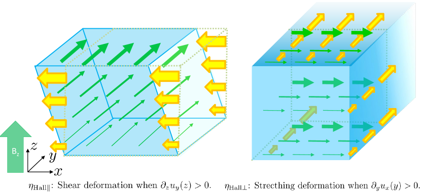
Figure 5: Hall viscosities induced by the Lorentz force exerting on charged fluid cells. The flow velocity and the Lorentz force are shown with green and orange arrows, respectively. The length and thickness of the arrows denote the magnitudes of the vectors. The direction of a magnetic field is taken along the $z$ direction.

We briefly demonstrate the mechanisms that generate the Hall viscosities in magnetic fields (assuming that there is a possible electric-charge density). In Fig. 5, the direction of a magnetic field is taken along the $z$ direction, and the flow velocity and the Lorentz force are shown with green and orange arrows, respectively. When there is a gradient of the transverse flow along the magnetic field $\partial_{z}u_{x}(z)>0$, the Lorentz force exerting on the fluid volume is oriented in the $y$ direction and has a gradient along the magnetic field (see the left panel). This configuration corresponds to the term proportional to $\eta_{H\parallel}$. The gradient of the Lorentz force gives rise to a shear stress in the plane orthogonal to the flow-velocity and magnetic fields. On the other hand, when there is a flow gradient in the transverse plane $\partial_{y}u_{x}(y)>0$, the Lorentz force is oriented in the $y$ direction and has a gradient in the same direction (see the right panel). Therefore, the fluid volume is stretched in this direction according to the term proportional to $\eta_{H\perp}$. This term also induces a shear deformation in the $x$-$y$ plane in response to an expansion/compression in the $x$ direction, $\partial_{x}u_{x}(x)\not=0$. This effect can be understood in a similar manner.

In the nonrelativistic theory, it has been known for some time that there are seven viscous coefficients Hooyman et al. (1954); Lifschitz and Pitaevskii (1981) (see also Ref. De Groot and Mazur (1962)). In this paper, we have obtained the breakdown of the seven viscous coefficients in the relativistic extension. Including the five dissipative viscosities discussed in the previous sections, we identified three bulk, two shear, and two Hall composnents. The relativistic extension was also carried out earlier in Refs. Huang et al. (2011); Hernandez and Kovtun (2017); Grozdanov et al. (2017); Hongo and Hattori (2021). However, those authors use different tensor bases. For readers’ convenience, we provide an explicit comparison among those tensor bases in Appendix D.

V Towards relativistic MHD from kinetic equations

In addition to hydrodynamics, kinetic theory is also often used for the studies of many-body systems (See Refs. Lifschitz and Pitaevskii (1981); de Groot et al. (1980) for the standard textbooks of kinetic theory). It is valid in the regime where the system permits well-defined particles (or quasi-particles) and when the densities of these particles are low enough. More precisely, let the typical microscopic scales be set by the interaction range $r_{c}\sim\sqrt{\sigma}$ with $\sigma$ the scattering cross section, the inter-particle distance $r_{d}\sim n^{-1/3}$ with $n$ the number density, and the mean-free path $\lambda_{\rm mfp}\sim 1/(n\sigma)$. The applicability of kinetic theory requires $\lambda_{\rm mfp}\gg r_{d}\gg r_{c}$ (dilute condition). The scatterings of the particles drive the system to evolve towards global thermal equilibrium, a process called kinetic thermalization. This process is usually associated with the arising of a new, macroscopic scale, $L$, over which the macroscopic properties of the system vary. In the late stage of the thermalization, the scale $L$ will be clearly separated from the microscopic scales. This gives a characteristic parameter ${\rm Kn}=\lambda_{\rm mfp}/L$ (the Knudsen number). When ${\rm Kn}\ll 1$ or equivalently when the derivative $\partial$ is much smaller than $1/\lambda_{\rm mfp}$, the macroscopic properties become insensitive to the microscopic details of the system and the hydrodynamic description is expected to arise. Therefore, when the kinetic theory is applied to the regime where ${\rm Kn}\ll 1$, its solution is expected to be expressed by the local hydrodynamic variables and their derivatives. This gives a systematical way to derive the hydrodynamic constitutive relations (including expressing the transport coefficients in terms of kinetic-theory parameters) and EOMs by expanding the kinetic equation and the distribution functions in ${\rm Kn}$ or $\partial$. This is the essential idea of the Chapman-Enskog method Chapman and Cowling (1970) which we will now discuss. Another frequently utilized approach to hydrodynamics from kinetic theory is the Grad’s method of moments Grad (1949) which we will explore in Sec. V.2.

V.1 Chapman-Enskog method

Before studying RMHD using kinetic theory, in order to demonstrate the methodology, let us consider a simpler case in which the EM fields are absent. The starting point is the relativistic Boltzmann equation for on-shell particles:

$$k^{\mu}\partial_{\mu}f_{{\bm{k}}}=C[f],$$ (91)

where $k^{\mu}=(k^{0}=\sqrt{{\bm{k}}^{2}+m^{2}},{\bm{k}})$ with $m$ being the mass of the particles, $f_{\bm{k}}(x)$ is the distribution function, and all external forces are omitted. For the sake of simplicity, we consider only one species of particles. We assume that the collisional process conserves the energy-momentum and also the particle numbers, so that the collision kernel satisfies

$$\int dKC[f]=\int dKk^{\mu}C[f]=0,$$ (92)

where $dK=gd^{3}{\bm{k}}/[(2\pi)^{3}k^{0}]$ is the invariant momentum-space measure with $g=2S+1$ the spin degenerate factor with $S$ spin of the particles. By using Eq. (91), Eq. (92) leads to the conservation of particle-number current $N^{\mu}$ and energy-momentum tensor $T^{\mu\nu}$,

$$\partial_{\mu}N^{\mu} = 0,$$ (93a)

$$\partial_{\mu}T^{\mu\nu} = 0,$$ (93b)

where $N^{\mu}$ and $T^{\mu\nu}$ are expressed by

$$N^{\mu} = \langle k^{\mu}\rangle=nu^{\mu}+\nu^{\mu},$$ (94a)

$$T^{\mu\nu} = \langle k^{\mu}k^{\nu}\rangle=\epsilon u^{\mu}u^{\nu}-\Delta^{\mu\nu}(p+\Pi)+h^{\mu}u^{\nu}+h^{\nu}u^{\mu}+\pi^{\mu\nu},$$ (94b)

with $\langle\cdots\rangle=\int dK(\cdots)f_{\bm{k}}$. Here, we introduced a timelike unit vector field $u^{\mu}$ which will be identified as the fluid velocity. Using $u^{\mu}$, the momentum can be decomposed into two parts (following the notations of Ref. Denicol et al. (2012a)): $k^{\mu}=E_{\bm{k}}u^{\mu}+k^{\langle\mu\rangle}$, with $E_{\bm{k}}=u\cdot k$ and $k^{\langle\mu\rangle}=\Delta^{\mu\nu}k_{\nu}$. We have also introduced the number density $n$, the number diffusion current $\nu^{\mu}$, the energy density $\epsilon$, the thermodynamic pressure $p$, the viscous pressure $\Pi$, the shear viscous tensor $\pi^{\mu\nu}$, and the heat flux $h^{\mu}$,

$$n=\langle E_{\bm{k}}\rangle,\;\nu^{\mu}=\langle k^{\langle\mu\rangle}\rangle,\;\epsilon=\langle E_{\bm{k}}^{2}\rangle,\;p+\Pi=-\frac{1}{3}\Delta^{\mu\nu}\langle k_{\mu}k_{\nu}\rangle,\;\pi^{\mu\nu}=\langle k^{\langle\mu}k^{\nu\rangle}\rangle,\;h^{\mu}=\langle E_{\bm{k}}k^{\langle\mu\rangle}\rangle,$$

where $A^{\langle\mu\nu\rangle}=(1/2)\Delta^{\mu}_{\alpha}\Delta^{\nu}_{\beta}(A^{\alpha\beta}+A^{\beta\alpha})-(1/3)\Delta^{\mu\nu}\Delta_{\alpha\beta}A^{\alpha\beta}$ is the spatial traceless symmetrization of $A^{\mu\nu}$. The expression for $p$ itself will be determined later. To specify the rest frame of the fluid, we use the Landau-Lifshitz choice so that $T^{\mu\nu}u_{\nu}=\epsilon u^{\mu}$. This imposes the constraint

$$h^{\mu}=\langle E_{\bm{k}}k^{\langle\mu\rangle}\rangle=0.$$ (96)

To proceed, one takes the Chapman-Enskog expansion of the distribution function, $f_{\bm{k}}=f^{(0)}_{{\bm{k}}}+f_{{\bm{k}}}^{(1)}+\cdots$, and of the Boltzmann equation (91) order by order in ${\rm Kn}$ or equivalently in derivatives. At zeroth order in the derivative expansion, Eq. (91) reads

$$0=C[f^{(0)}].$$ (97)

Its solution is called the local-equilibrium distribution $f^{(0)}_{\bm{k}}=f_{0{\bm{k}}}$ because it saturates the local detailed balance. We assume that $f_{0{\bm{k}}}=1/[\exp(\beta E_{\bm{k}}-\alpha)+a]$ with $a=1,0$ and $-1$ for fermions, classical Boltzmann particles, and bosons. Here, $\beta$ and $\alpha=\beta\mu$ are the local inverse temperature and the ratio of the chemical potential to temperature. Their values are fixed by matching conditions Stewart (1971); de Groot et al. (1980):

$$\epsilon=\langle E_{\bm{k}}^{2}\rangle=\langle E_{\bm{k}}^{2}\rangle_{0},\;\;n=\langle E_{\bm{k}}\rangle=\langle E_{\bm{k}}\rangle_{0},$$ (98)

where $\langle\cdots\rangle_{0}=\int dK(\cdots)f_{0{\bm{k}}}$. Substituting $f_{0{\bm{k}}}$ into Eqs. (94a) and (94b), one obtains the zeroth-order $N^{\mu}$ and $T^{\mu\nu}$:

$$N_{(0)}^{\mu} = nu^{\mu},$$ (99a)

$$T_{(0)}^{\mu\nu} = \epsilon u^{\mu}u^{\nu}-p\Delta^{\mu\nu},$$ (99b)

where $p=-\frac{1}{3}\Delta^{\mu\nu}\langle k_{\mu}k_{\nu}\rangle_{0}$, and Eqs. (93a) and (93b) become the ideal hydrodynamic equations.

At first order in derivative expansion, the collision kernel becomes a linear integral operator acting on $f_{\bm{k}}^{(1)}$, $C^{(1)}[f]=\hat{L}f_{\bm{k}}^{(1)}$. The Boltzmann equation (91) at $O({\rm Kn})$ thus reads

$$k^{\mu}\partial_{\mu}f_{0{\bm{k}}}=\hat{L}f_{\bm{k}}^{(1)}.$$ (100)

Once $f_{\bm{k}}^{(1)}$ is solved out from this equation, the first-order constitutive relations are then obtained:

$$\nu^{\mu}=\langle k^{\langle\mu\rangle}\rangle_{1},\;\Pi=-\frac{1}{3}\Delta^{\mu\nu}\langle k_{\mu}k_{\nu}\rangle_{1},\;\pi^{\mu\nu}=\langle k^{\langle\mu}k^{\nu\rangle}\rangle_{1},$$ (101)

with $\langle\cdots\rangle_{1}=\int dK(\cdots)f^{(1)}_{{\bm{k}}}$. To see how this procedure works in practice, let us consider a collision kernel in relaxation-time approximation (RTA) ,

$$C[f]=-E_{\bm{k}}\frac{f_{\bm{k}}-f_{0{\bm{k}}}}{\tau_{R}}.$$ (102)

Writing $f^{(1)}_{\bm{k}}$ as $f^{(1)}_{\bm{k}}=f_{0{\bm{k}}}\tilde{f}_{0{\bm{k}}}\phi_{\bm{k}}$ with $\phi_{\bm{k}}$ at $O({\rm Kn})$ and $\tilde{f}_{\bm{k}}=1-af_{\bm{k}}$, one obtains ${\hat{L}}f^{(1)}_{\bm{k}}=-\tau_{R}^{-1}E_{\bm{k}}f_{0{\bm{k}}}\tilde{f}_{0{\bm{k}}}\phi_{\bm{k}}$. From Eq. (100), one finds

$$\phi_{\bm{k}}=\frac{\beta\tau_{R}}{E_{\bm{k}}}\bigg{[}\left(\frac{1}{3}\Delta_{\mu\nu}k^{\mu}k^{\nu}+E^{2}_{\bm{k}}\frac{\partial p}{\partial\epsilon}\Big{|}_{n}+E_{\bm{k}}\frac{\partial p}{\partial n}\Big{|}_{\epsilon}\right)\theta+T\left(\frac{nE_{\bm{k}}}{\epsilon+p}-1\right)k^{\mu}\nabla_{\mu}\alpha+k^{\langle\mu}k^{\nu\rangle}\xi_{\mu\nu}\bigg{]},$$

where we defined $\xi_{\mu\nu}:=w_{\langle\mu\nu\rangle}$ which is the shear tensor , and the terms are organized in such a way that they are mutually orthogonal under integral $\int dK(\cdots)F(E_{\bm{k}})$ with $F(E_{\bm{k}})$ an arbitrary converging function of $E_{\bm{k}}$. Substituting $\phi_{\bm{k}}$ into Eq. (101), one finds

$$\nu^{\mu} = \kappa\,\nabla^{\mu}\alpha,\quad{\rm with}\quad\kappa=\tau_{R}T\left(\frac{2}{3}\frac{\epsilon-3p}{m^{2}}-\frac{n^{2}}{\epsilon+p}+\frac{m^{2}}{3}\left\langle\frac{1}{E_{\bm{k}}^{2}}\right\rangle_{0}\right),\,$$ (104a)

$$\Pi = -\zeta\,\theta,\quad{\rm with}\quad\zeta=\tau_{R}\left[\left(\frac{1}{3}-c_{s}^{2}\right)(\epsilon+p)-\frac{2}{9}(\epsilon-3p)-\frac{m^{4}}{9}\left\langle\frac{1}{E_{\bm{k}}^{2}}\right\rangle_{0}\right],\,$$ (104b)

$$\pi^{\mu\nu} = 2\eta\,\xi^{\mu\nu},\quad{\rm with}\quad\eta=\tau_{R}\left[\frac{4}{5}p+\frac{1}{15}(\epsilon-3p)-\frac{m^{4}}{15}\left\langle\frac{1}{E_{\bm{k}}^{2}}\right\rangle_{0}\right],\,$$ (104c)

where $c_{s}^{2}=\partial p/\partial\epsilon|_{s/n}=\partial p/\partial\epsilon|_{n}+(\epsilon+p)^{-1}n\,\partial p/\partial n|_{\epsilon}$ is the sound velocity squared, $\kappa,\zeta,\eta$ are conductivity of number diffusion current, bulk viscosity, and shear viscosity. Note that when $m=0$, the bulk viscosity vanishes because $\epsilon=3p$ and $c_{s}^{2}=1/3$ in massless limit. Thus, at $O({\rm Kn})$, we recover the relativistic Navier-Stokes hydrodynamics.

With the above preparation, let us now consider RMHD in the Chapman-Enskog method. In this case, the Boltzmann equation contains the EM force term:

$$k^{\mu}\partial_{\mu}f_{{\bm{k}}}+qF^{\mu\nu}k_{\nu}\partial_{k^{\mu}}f_{\bm{k}}=C[f],$$ (105)

where $q$ is the charge of the particles (we consider only one species of particles and assume $q>0$). We assume that the particles are under binary elastic collisions and the colliding processes are not interfered by the external EM field $F^{\mu\nu}$. Hence the collision kernel preserves the particle number (and the electric charges as well) and energy-momentum, i.e., Eq. (92) still holds which implies

$$\partial_{\mu}N^{\mu} = \partial_{\mu}\int dKk^{\mu}f_{\bm{k}}=0,$$ (106)

$$\partial_{\mu}T^{\mu\nu} = \partial_{\mu}\int dKk^{\mu}k^{\lambda}f_{\bm{k}}=qF^{\nu\lambda}N_{\lambda}=F^{\nu\lambda}J_{\lambda},$$ (107)

where $J^{\mu}=qN^{\mu}$ is the charge current. We emphasize that the EM fields appear in our kinetic approach as external fields which is very different from Sec. II and Sec. III in which the dynamics of the EM fields plays important role. This leads to different leading-order constitutive relations, but they share the same structures of the dissipative constitutive relations for the fluid (namely, the viscous and conductivity tensors).

Let us clarify a significant distinction between how the EM fields are treated in this section and how they are treated in Sec. II and Sec. III. In Sec. II and Sec. III, the EM fields are dynamical and the energy-momentum tensor includes contributions from the EM fields as well, resulting in a conserved energy-momentum tensor. The RMHD derived in Sec. II and Sec. III is therefore a strict hydrodynamic theory. This is not the case with this section, where the EM fields are external fields (as clearly seen in Eq. (105)), hence $N^{\mu}$ and $T^{\mu\nu}$ obtained from the kinetic theory only include contributions from the matter. As shown in the right-hand side of Eq. (107), matter exchanges energy and momentum with EM fields, causing the $T^{\mu\nu}$ to be non-strictly conserved. For this reason, the pressure and energy density include only the matter contributions.

The presence of the EM fields introduces new scales into the kinetic equation (and also the hydrodynamic equations). So let us clarify the range of scales that we will focus in this case. The typical microscopic scales are still set by the interaction range $r_{c}$, inter-particle distance $r_{d}$, and the mean-free path $\lambda_{\rm mfp}$. In terms of ${\rm Kn}$ or the gradient $\partial$ of the conserved densities, the electric field in the rest frame of the fluid, $E^{\mu}=F^{\mu\nu}u_{\nu}$, is considered as $O(\partial)$, while the magnetic field in the rest frame of the fluid, $B^{\mu}=\varepsilon^{\mu\nu\alpha\beta}u_{\nu}F_{\alpha\beta}/2$, can be an $O(1)$ quantity, as we already emphasized in Sec. II. This amounts to the fact that the electric field is screened by the gradient of charge distribution in a plasma, while magnetic field is not. The magnetic field makes the motion of charged particles curvilinear with radius $R_{L}=k_{\perp}/(qB)$ (the Larmor radius) with $k_{\perp}$ being the momentum of the particles transverse to the magnetic field. For hot relativistic plasma, $k_{\perp}\sim T$; so $R_{T}=T/(qB)$ sets the magnetic cyclotron scale. We will always assume that the thermal wavelength $\beta=1/T$ of the particles and the interaction range $r_{c}$ are much smaller than $R_{T}$, $\beta\ll R_{T}$ and $r_{c}\ll R_{T}$. The first inequality means that the Landau quantization effect is not significant and we can safely use a classical treatment. The second inequality means that in the collision process the magnetic field can be neglected so we can use a magnetic-field independent collision operator C (but the distribution function $f_{\bm{k}}$ can certainly depend on $B^{\mu}$). The situation with an even stronger magnetic field, $R_{T}\ll\beta$, that can make the Landau quantization effect significant, will be discussed in Sec. VI.

We will always use the Landau-Lifshitz frame for the fluid and use the matching conditions for $\epsilon$ and $n$. The zeroth-order distribution function is still chosen as $f^{(0)}_{\bm{k}}=f_{0{\bm{k}}}=1/[\exp(\beta E_{\bm{k}}-\alpha)+a]$ with $a=1,0$ and $-1$ for fermions, classical Boltzmann particles, and bosons. Choosing such an equilibrium distribution amounts to assume that the magnetization pressure $-MB$ is much smaller than thermodynamic pressure $p$ and thus is omitted. This also implies that the magnetization current is vanishing and we thus do not distinguish the free electric current and the total electric current in this section. Therefore, the ideal-fluid constitutive relations are still given by Eqs. (99a) and (99b). To obtain $f^{(1)}_{\bm{k}}$, let us again take the RTA for the collision kernel,

$$C[f]=-E_{\bm{k}}\frac{f_{\bm{k}}-f_{0{\bm{k}}}}{\tau_{R}}.$$ (108)

First, we consider a situation in which both $E^{\mu}$ and $B^{\mu}$ in Eq. (105) are of order $O(\partial)$, namely, when both the electric and magnetic fields are very weak. This is not in the MHD region but let us make a case study first. Writing $f^{(1)}_{\bm{k}}$ as $f^{(1)}_{\bm{k}}=f_{0{\bm{k}}}\tilde{f}_{0{\bm{k}}}\phi_{\bm{k}}$ with $\phi_{\bm{k}}$ at $O({\partial})$ and $\tilde{f}_{\bm{k}}=1-af_{\bm{k}}$, one obtains from Eq. (105),

$$\phi_{\bm{k}} = -\frac{\tau_{R}}{E_{\bm{k}}}(f_{0{\bm{k}}}\tilde{f}_{0{\bm{k}}})^{-1}\left(k^{\mu}\partial_{\mu}f_{0{\bm{k}}}+qF^{\mu\nu}k_{\nu}\partial_{k^{\mu}}f_{0{\bm{k}}}\right)$$ (109)

$$= \frac{\beta\tau_{R}}{E_{\bm{k}}}\bigg{[}T\left(\frac{nE_{\bm{k}}}{\epsilon+p}-1\right)k^{\mu}\left(\nabla_{\mu}\alpha+\beta qE_{\mu}\right)$$

$$+\left(\frac{1}{3}\Delta_{\mu\nu}k^{\mu}k^{\nu}+E^{2}_{\bm{k}}\frac{\partial p}{\partial\epsilon}\Big{|}_{n}+E_{\bm{k}}\frac{\partial p}{\partial n}\Big{|}_{\epsilon}\right)\theta+k_{\perp}^{\langle\mu}k_{\perp}^{\nu\rangle}\xi_{\mu\nu}\bigg{]}.$$

Compared with Eq. (V.1), the only new term is the electric-field term which is always accompanied with $\nabla_{\mu}\alpha$ and the magnetic field drops out. To obtain $\phi_{\bm{k}}$, we have used the EOMs at $O(1)$ order (ideal hydrodynamic equations):

$$Du^{\mu} = \frac{1}{\epsilon+p}\left(\nabla^{\mu}p+nqE^{\mu}\right),$$ (110)

$$D\alpha = -\beta\frac{\partial p}{\partial n}\Big{|}_{\epsilon}\theta,$$ (111)

$$D\beta = \beta\frac{\partial p}{\partial\epsilon}\Big{|}_{n}\theta.$$ (112)

Substituting $f^{(1)}_{\bm{k}}$ into Eqs. (101), we find that the $\Pi$ and $\pi^{\mu\nu}$ are still given by Eqs. (104b) and (104c) but $\nu^{\mu}$ is given by $\nu^{\mu}=\kappa\left(\nabla^{\mu}\alpha+\beta qE^{\mu}\right)$ with the number diffusion constant $\kappa$ given in Eq. (104a). The charge diffusion current $j^{\mu}=q\langle k^{\langle\mu\rangle}\rangle_{1}$ is

$$j^{\mu}=q\nu^{\mu}=q\kappa\left(\nabla^{\mu}\alpha+\beta qE^{\mu}\right).$$ (113)

This relation gives that the electric conductivity (the coefficient in front of $E^{\mu}$) is determined by number diffusion conductivity, $\sigma=\beta q^{2}\kappa$, a relation representing the Wiedemann–Franz law.

The above situation with $B^{\mu}\sim O(\partial)$ is not in the MHD region. Let us now consider the MHD region in which $E^{\mu}$ is at $O(\partial)$ but $B^{\mu}$ is at $O(1)$. The Boltzmann equation at $O(\partial)$ reads

$$k^{\mu}\partial_{\mu}f_{0{\bm{k}}}-qE^{\nu}k_{\nu}u^{\mu}\partial_{k^{\mu}}f_{0{\bm{k}}}=-qBb_{\star}^{\mu\nu}k_{\nu}\partial_{k^{\mu}}f^{(1)}_{\bm{k}}-\frac{E_{\bm{k}}}{\tau_{R}}f^{(1)}_{\bm{k}},$$ (114)

where $B=\sqrt{-B^{\mu}B_{\mu}}$ is the strength of the magnetic field and $b_{\star}^{\mu\nu}=\varepsilon^{\mu\nu\alpha\beta}u_{\alpha}b_{\beta}$ is the cross projector. The solution for $f^{(1)}_{\bm{k}}$ is $f^{(1)}_{\bm{k}}=f_{0{\bm{k}}}\tilde{f}_{0{\bm{k}}}\phi_{\bm{k}}$ with

$$\phi_{\bm{k}} = \phi_{\parallel}+\frac{\tau_{R}}{E_{\bm{k}}}\frac{\beta}{1+\xi_{\bm{k}}^{2}}\left(V^{\mu}+\xi_{\bm{k}}b_{\star}^{\mu\nu}V_{\nu}\right)k^{\perp}_{\mu}+\frac{\tau_{R}}{E_{\bm{k}}}\frac{\beta}{1+4\xi_{\bm{k}}^{2}}\left(w_{\perp}^{\mu\nu}+2\xi_{\bm{k}}b_{\star}^{\mu\lambda}w^{\nu}_{\perp\lambda}\right)k^{\perp}_{\{\mu}k^{\perp}_{\nu\}},$$ (115)

$$\phi_{\parallel} = \frac{\beta\tau_{R}}{E_{\bm{k}}}\bigg{[}\left(\frac{1}{2}\Xi_{\alpha\beta}k^{\alpha}k^{\beta}+E^{2}_{\bm{k}}\frac{\partial p}{\partial\epsilon}\Big{|}_{n}+E_{\bm{k}}\frac{\partial p}{\partial n}\Big{|}_{\epsilon}\right)\theta_{\perp}+\left(-k_{\parallel}^{2}+E^{2}_{\bm{k}}\frac{\partial p}{\partial\epsilon}\Big{|}_{n}+E_{\bm{k}}\frac{\partial p}{\partial n}\Big{|}_{\epsilon}\right)\theta_{\parallel}$$ (116)

$$-Tk_{\parallel}\left(\frac{nE_{\bm{k}}}{\epsilon+p}-1\right)b^{\mu}\left(\nabla_{\mu}\alpha+\beta qE_{\mu}\right)\bigg{]},$$

$$V^{\mu} = \left[T\left(\frac{nE_{\bm{k}}}{\epsilon+p}-1\right)\Xi^{\mu\lambda}\left(\nabla_{\lambda}\alpha+\beta qE_{\lambda}\right)-2k_{\parallel}\Xi^{\mu\lambda}w_{\lambda\rho}b^{\rho}+\frac{qB}{\epsilon+p}E_{\bm{k}}b_{\star}^{\mu\lambda}\nu_{\lambda}\right],$$ (117)

where $\xi_{\bm{k}}:=qB\tau_{R}/E_{\bm{k}}$ and we have introduced

$$\begin{split}&k_{\parallel}=b\cdot k,\;\;\Xi^{\mu\nu}=\Delta^{\mu\nu}+b^{\mu}b^{\nu},\;\;k_{\perp}^{\mu}=\Xi^{\mu\nu}k_{\nu},\;\;k_{\perp}^{\{\mu}k_{\perp}^{\nu\}}=k_{\perp}^{\mu}k_{\perp}^{\nu}-\frac{1}{2}\Xi^{\mu\nu}\Xi_{\alpha\beta}k^{\alpha}k^{\beta},&\;\\ &w_{\mu\nu}=\frac{1}{2}(\nabla_{\mu}u_{\nu}+\nabla_{\nu}u_{\mu}),\;\;\theta_{\perp}=\Xi_{\alpha\beta}w^{\alpha\beta},\;\;\theta_{\parallel}=-b_{\mu}b_{\nu}w^{\mu\nu},\;\;w_{\perp}^{\mu\nu}=\left(\Xi^{\mu\alpha}\Xi^{\nu\beta}-\frac{1}{2}\Xi^{\mu\nu}\Xi^{\alpha\beta}\right)w_{\alpha\beta}.&\end{split}$$ (118)

Note that to derive Eq. (115) we use again Eqs. (110)-(112) but Eq. (110) is replaced by

$$Du^{\mu} = \frac{1}{\epsilon+p}\left(\nabla^{\mu}p+nqE^{\mu}+qBb_{\star}^{\mu\lambda}\nu_{\lambda}\right),$$ (119)

because now $B^{\mu}\sim O(1)$ and is kept in the ideal EOMs.

We can check explicitly that the matching conditions $\langle E_{\bm{k}}\rangle_{1}=0,\langle E_{\bm{k}}^{2}\rangle_{1}=0$ are satisfied with $f^{(1)}_{\bm{k}}$. The Landau-Lifshitz frame-fixing condition $\langle E_{\bm{k}}k^{\langle\mu\rangle}\rangle_{1}=0$ is, however, not satisfied. In fact, because $f^{(1)}_{\bm{k}}$ depends on $\nu^{\mu}$ explicitly, the Landau-Lifshitz condition must be coupled with the defining condition for $\nu^{\mu}$ to determine $u^{\mu}$ and $\nu^{\mu}$. A simpler way to solve out $\nu^{\mu}$ from these complicated coupled equations is by considering the frame-independent vector (See Appendix B for the discussion of the transformation among different choices of the fluid velocity)

$$l^{\mu}=\langle k^{\langle\mu\rangle}\rangle_{1}-\frac{n}{\epsilon+p}\langle E_{\bm{k}}k^{\langle\mu\rangle}\rangle_{1},$$ (120)

which depends on $\nu^{\mu}$ and should equal to $\nu^{\mu}$ once the Landau-Lifshitz condition is fulfilled. Therefore, $\nu^{\mu}$ in the Landau-Lifshitz frame should be determined by

$$\nu^{\mu}=\langle k^{\langle\mu\rangle}\rangle_{1}-\frac{n}{\epsilon+p}\langle E_{\bm{k}}k^{\langle\mu\rangle}\rangle_{1}.$$ (121)

This is a linear equation for $\nu^{\mu}$ and can be directly solved. To demonstrate this and for simplicity of the discussion, we assume that the magnetic cyclotron frequency $\omega_{B}=1/R_{T}=qB/T$ is much larger than the collision rate $\omega_{\rm col}=1/\tau_{R}$ (or equivalently, $\xi=\lambda_{\rm mfp}/R_{T}\gg 1$). In this case, $\xi_{\bm{k}}\sim\xi\gg 1$ and we can expand $f^{(1)}_{\bm{k}}$ in $1/\xi_{\bm{k}}$. Solving Eq. (121) order by order in $1/\xi$, we obtain

$$\nu^{\mu} = \kappa^{\mu\nu}\left(\partial_{\nu}\alpha+\beta qE_{\nu}\right),$$ (122)

$$\kappa^{\mu\nu} = \kappa_{\perp}\Xi^{\mu\nu}-\kappa_{\parallel}b^{\mu}b^{\nu}+\kappa_{H}b_{\star}^{\mu\nu},$$ (123)

where the conductivities read

$$\kappa_{\perp} = \frac{1}{\tau_{R}(qB)^{2}}\frac{\epsilon+p}{\beta}\left(\frac{J_{31}J_{51}}{J_{41}^{2}}-1\right)+O(\xi^{-4})=\frac{1}{\tau_{R}(qB)^{2}}\frac{J_{31}D_{41}}{J^{2}_{41}}+O(\xi^{-4}),$$ (124a)

$$\kappa_{\parallel} = \tau_{R}\left(J_{11}-\frac{n}{\epsilon+p}J_{21}\right)=\tau_{R}\frac{D_{21}}{J_{31}},$$ (124b)

$$\kappa_{H} = \frac{1}{qB}\left(\frac{n}{\beta}-\frac{J_{31}^{2}}{J_{41}}\right)+O(\xi^{-3})=\frac{1}{qB}\frac{D_{31}}{J_{41}}+O(\xi^{-3}).$$ (124c)

We have introduced the thermodynamic functions $J_{nq}$ and $D_{nq}$ to simplify the expressions. For the later use, we also introduce another two thermodynamic functions $I_{nq}$ and $G_{nm}$. They are defined by Denicol et al. (2012a)

$$I_{nq} = \frac{(-1)^{q}}{(2q+1)!!}\int dKE_{\bm{k}}^{n-2q}(\Delta_{\alpha\beta}k^{\alpha}k^{\beta})^{q}f_{0{\bm{k}}},$$ (125a)

$$J_{nq} = \frac{(-1)^{q}}{(2q+1)!!}\int dKE_{\bm{k}}^{n-2q}(\Delta_{\alpha\beta}k^{\alpha}k^{\beta})^{q}f_{0{\bm{k}}}\tilde{f}_{0{\bm{k}}},$$ (125b)

$$D_{nq} = J_{n+1,q}J_{n-1,q}-J_{nq}^{2},$$ (125c)

$$G_{nm} = J_{n0}J_{m0}-J_{n-1,0}J_{m+1,0},$$ (125d)

where $J_{nq}$ and $I_{nq}$ are related by $\beta J_{nq}=I_{n-1,q-1}+(n-2q)I_{n-1,q}$. Note that $\kappa_{\parallel}=\kappa$ in Eq. (104a) (which can be directly shown using Eq. (125b)), meaning that the charge diffusion along the magnetic field is unaffected by the magnetic field. Note that the leading-order Hall conductivity $\kappa_{H}$ is independent of the relaxation time $\tau_{R}$; it is purely due to the Lorentz force. The first term in $\kappa_{H}$ gives the classical Hall conductivity for a stationary material while the second term is due to the fluid flow and thus depends on how we approximate the dynamic kinetic and hydrodynamic equations.

Substituting $f^{(1)}_{\bm{k}}$ into $\tau^{\mu\nu}:=\langle k^{\langle\mu\rangle}k^{\langle\nu\rangle}\rangle_{1}=\pi^{\mu\nu}-\Delta^{\mu\nu}\Pi$, we obtain the viscous stress tensor $\tau^{\mu\nu}$ as

$$\tau^{\mu\nu} = \sum_{i=1}^{7}\eta_{i}\eta^{\mu\nu\rho\sigma}_{i}w_{\rho\sigma},$$ (126)

where the tensor forms of $\eta^{\mu\nu\rho\sigma}_{i}$ are already defined in Eq. (II.2.3) and Eq. (90) but listed here for convenience

$$\eta^{\mu\nu\rho\sigma}_{1} = b^{\mu}b^{\nu}b^{\rho}b^{\sigma},$$ (127a)

$$\eta^{\mu\nu\rho\sigma}_{2} = \Xi^{\mu\nu}\Xi^{\rho\sigma},$$ (127b)

$$\eta^{\mu\nu\rho\sigma}_{3} = -\Xi^{\mu\nu}b^{\rho}b^{\sigma}-\Xi^{\rho\sigma}b^{\mu}b^{\nu},$$ (127c)

$$\eta^{\mu\nu\rho\sigma}_{4} = -2\left[b^{(\mu}\Xi^{\nu)\rho}b^{\sigma}+b^{(\mu}\Xi^{\nu)\sigma}b^{\rho}\right],$$ (127d)

$$\eta^{\mu\nu\rho\sigma}_{5} = 2\,\Xi^{\rho(\mu}\Xi^{\nu)\sigma}-\Xi^{\mu\nu}\Xi^{\rho\sigma},$$ (127e)

$$\eta^{\mu\nu\rho\sigma}_{6} = -b^{(\mu}b_{\star}^{\nu)\rho}b^{\sigma}-b^{(\mu}b_{\star}^{\nu)\sigma}b^{\rho},$$ (127f)

$$\eta^{\mu\nu\rho\sigma}_{7} = \Xi^{\rho(\mu}b_{\star}^{\nu)\sigma}+\Xi^{\sigma(\mu}b_{\star}^{\nu)\rho},$$ (127g)

and the viscosities are given by

$$\eta_{1} := \zeta_{\parallel}=\beta\tau_{R}\left(3J_{32}-J_{31}\frac{\partial p}{\partial\epsilon}\Big{|}_{n}-J_{21}\frac{\partial p}{\partial n}\Big{|}_{\epsilon}\right),$$ (128a)

$$\eta_{2} := \zeta_{\perp}=\beta\tau_{R}\left(2J_{32}-J_{31}\frac{\partial p}{\partial\epsilon}\Big{|}_{n}-J_{21}\frac{\partial p}{\partial n}\Big{|}_{\epsilon}\right),$$ (128b)

$$\eta_{3} := \zeta_{\times}=\beta\tau_{R}\left(J_{32}-J_{31}\frac{\partial p}{\partial\epsilon}\Big{|}_{n}-J_{21}\frac{\partial p}{\partial n}\Big{|}_{\epsilon}\right),$$ (128c)

$$\eta_{4} := \eta_{\parallel}=\frac{\beta}{\tau_{R}(qB)^{2}}J_{52}+O(\xi^{-4}),$$ (128d)

$$\eta_{5} := \eta_{\perp}=\frac{\beta}{4\tau_{R}(qB)^{2}}J_{52}+O(\xi^{-4}),$$ (128e)

$$\eta_{6} := \eta_{H\parallel}=\frac{2\beta}{qB}J_{42}+O(\xi^{-3}),$$ (128f)

$$\eta_{7} := \eta_{H\perp}=\frac{\beta}{2qB}J_{42}+O(\xi^{-3}),$$ (128g)

where $\zeta$’s and $\eta$’s are bulk and shear viscosities whose physical meaning has been discussed in Sec. II.2. The above result automatically satisfies the Onsager relation for $\zeta_{\times}$ that was assumed in Sec. II.2. Note that $\eta_{H\parallel}$ and $\eta_{H\perp}$ do not depend on $\tau_{R}$ at the leading order in $1/\xi$; they arise due to the Lorentz force and are thus called Hall viscosities; see more discussions in Sec. IV.2.

For massless Boltzmann gas, using $J_{nq}=(n+1)!\beta^{2-n}p/[2(2q+1)!!]$ Denicol et al. (2018) and $\tau_{R}=9\lambda_{\rm mfp}/4$, the transport coefficients become

$$\begin{split}&\kappa_{\parallel}=\frac{3}{16}\lambda_{\rm mfp}n,\;\;\kappa_{\perp}=\frac{16}{45}\frac{\lambda_{\rm mfp}n}{\xi^{2}},\;\;\kappa_{H}=\frac{1}{5}\frac{n}{\beta qB},\;\;\zeta_{\parallel}=\frac{12}{5}\lambda_{\rm mfp}p,\;\;\zeta_{\perp}=\frac{3}{5}\lambda_{\rm mfp}p,&\\ &\zeta_{\times}=-\frac{6}{5}\lambda_{\rm mfp}p,\;\;\eta_{\parallel}=\frac{32}{3}\frac{\lambda_{\rm mfp}p}{\xi^{2}},\;\;\eta_{\perp}=\frac{8}{3}\frac{\lambda_{\rm mfp}p}{\xi^{2}},\;\;\eta_{H\parallel}=\frac{8p}{\beta qB},\;\;\eta_{H\perp}=\frac{2p}{\beta qB}.&\end{split}$$ (129)

Note that $\zeta_{\parallel}\zeta_{\perp}-\zeta_{\times}^{2}=0$ due to the conformal invariance in 3-dimensional space in the massless limit.

Recently, there have been intensive use of the Chapman-Enskog method to study the constitutive relations and transport coefficients in RMHD; see Refs. Mohanty et al. (2019); Das et al. (2020); Dey et al. (2021b); Das et al. (2019); Chen et al. (2020); Dash et al. (2020); Rath and Patra (2021); Panda et al. (2021a, b); Rath and Dash (2021, 2022) (also, e.g. Refs. Satapathy et al. (2021); Ghosh and Ghosh (2021) for related Kubo-formula calculations). Our discussions here serve as a simple overview and summary of how the Chapman-Enskog method is used to derive the constitutive relations of the first-order RMHD. For more information, the reader is referred to the list of references for recent works.

The above iterative procedure of solving Boltzmann equation can continue to the higher orders in gradient, but the calculations become much more involved. For example, at the second order, one obtains the Burnett-type equations Burnett (1935, 1936). However, the relativistic EOMs from the Chapman-Enskog expansion are in general unstable Hiscock and Lindblom (1983, 1985, 1987); Denicol et al. (2008); Pu et al. (2010); Biswas et al. (2020) (though there could exist special rest frames where the first-order relativistic dissipative hydrodynamics can be stable; see Refs. Bemfica et al. (2018, 2019); Kovtun (2019); Bemfica et al. (2022); Hoult and Kovtun (2020); Armas and Camilloni (2022)). For the Burnett equations, even at the non-relativistic limit, they suffer from the so-called Bobylev instability Bobylev (1982). For this reason, instead, the method of moments are widely used in recent years because it can avoid this problem Betz et al. (2009); Denicol et al. (2010, 2012b, 2012a, 2012c).

V.2 Grad’s method of moments

This approach was first established by Grad for non-relativistic systems Grad (1949) that can be viewed as an expansion of the distribution function in terms of momenta $k^{\nu}$ and was then generalized to relativistic systems by Israel and Stewart Stewart (1971); Israel and Stewart (1976, 1979a, 1979b) among others. Recently, a variant of this method was developed and widely adopted to derive the causal second-order hydrodynamics Betz et al. (2009); Denicol et al. (2010, 2012b, 2012a, 2012c); Jaiswal (2013); Bazow et al. (2014); Denicol et al. (2014); Molnar et al. (2016); Molnár et al. (2016); Denicol et al. (2018, 2019); Tinti et al. (2019); Most et al. (2021); Wagner et al. (2022). The following discussions closely follow Refs. Denicol et al. (2012a, c, 2018, 2019). We first discuss the simpler situation without EM fields and then consider the effect of EM fields.

The ideal hydrodynamics is still generated by the local equilibrium distribution $f_{0{\bm{k}}}$. Write the dissipative part of the distribution function as ${\delta}f_{\bm{k}}=f_{\bm{k}}-f_{0{\bm{k}}}=f_{0{\bm{k}}}\tilde{f}_{0{\bm{k}}}\phi_{\bm{k}}$. In the method of moments, $\phi_{\bm{k}}$ is expanded as a series of the irreducible tensors $1,k^{\langle\mu\rangle},k^{\langle\mu}k^{\nu\rangle},k^{\langle\mu}k^{\nu}k^{\lambda\rangle},\cdots$, $\phi_{\bm{k}}=\sum_{l=0}^{M}\lambda^{\langle\mu_{1}\cdots\mu_{l}\rangle}(E_{\bm{k}})k_{\langle\mu_{1}}\cdots k_{\mu_{l}\rangle}$. These irreducible tensors are defined by $k^{\langle\mu_{1}}\cdots k^{\mu_{l}\rangle}=\Delta^{\mu_{1}\cdots\mu_{l}\nu_{1}\cdots\nu_{l}}k_{\nu_{1}}\cdots k_{\nu_{l}}$ and form a complete and orthogonal set in the spatial momentum space, satisfying Denicol et al. (2012a)

$$\int dKF(E_{\bm{k}})k^{\langle\mu_{1}}\cdots k^{\mu_{m}\rangle}k^{\langle\nu_{1}}\cdots k^{\nu_{n}\rangle}=\frac{m!{\delta}_{nm}}{(2m+1)!!}\Delta^{\mu_{1}\cdots\mu_{m}\nu_{1}\cdots\nu_{m}}\int dKF(E_{\bm{k}})(\Delta_{\alpha\beta}k^{\alpha}k^{\beta})^{m},\quad\quad\quad$$ (130)

where $(2m+1)!!$ is the double factorial, $F$ is an arbitrary converging scalar function, and $\Delta^{\mu_{1}\cdots\mu_{m}\nu_{1}\cdots\nu_{m}}$ is the projection $\Delta^{\mu\nu}$ when $m=1$ and the symmetrized spatial traceless projection when $m\geq 2$, e.g., $\Delta^{\mu\nu\alpha\beta}=\frac{1}{2}(\Delta^{\mu\alpha}\Delta^{\nu\beta}+\Delta^{\mu\beta}\Delta^{\nu\alpha})-\frac{1}{3}\Delta^{\mu\nu}\Delta^{\alpha\beta}$. The coefficients $\lambda^{\langle\mu_{1}\cdots\mu_{l}\rangle}(E_{\bm{k}})$ may be further expanded in $E_{\bm{k}}$, conveniently with an orthogonal basis of polynomials $P_{n}^{(l)}(E_{\bm{k}})$, $\lambda^{\langle\mu_{1}\cdots\mu_{l}\rangle}(E_{\bm{k}})=\sum_{n=0}^{N_{l}}c_{n}^{\langle\mu_{1}\cdots\mu_{l}\rangle}P_{n}^{(l)}(E_{\bm{k}})$ . The functions $P_{n}^{(l)}(E_{\bm{k}})$ are $n$-th order polynomials in $E_{\bm{k}}$, $P_{n}^{(l)}(E_{\bm{k}})=\sum_{r=0}^{n}a_{nr}^{(l)}E_{\bm{k}}^{r}$, where the coefficients $a_{nr}^{(l)}$ can be determined order by order using the orthonormality condition

$$\frac{{\mathcal{N}}^{(l)}}{(2l+1)!!}\int dK(\Delta_{\alpha\beta}k^{\alpha}k^{\beta})^{l}f_{0{\bm{k}}}\tilde{f}_{0{\bm{k}}}P_{n}^{(l)}(E_{\bm{k}})P_{m}^{(l)}(E_{\bm{k}})={\delta}_{nm},$$

where ${\mathcal{N}}^{(l)}=(2l+1)!!\left[\int dK(\Delta_{\alpha\beta}k^{\alpha}k^{\beta})^{l}f_{0{\bm{k}}}\tilde{f}_{0{\bm{k}}}\right]^{-1}$ are the normalization factors . The remaining coefficients $c_{n}^{\langle\mu_{1}\cdots\mu_{l}\rangle}$ can be more conveniently re-expressed using the irreducible moments,

$$\rho_{r}^{\mu_{1}\cdots\mu_{l}}:=\langle E_{\bm{k}}^{r}k^{\langle\mu_{1}}\cdots k^{\mu_{l}\rangle}\rangle_{\delta}=\int dKE_{\bm{k}}^{r}k^{\langle\mu_{1}}\cdots k^{\mu_{l}\rangle}{\delta}f_{\bm{k}},$$ (131)

as $c_{n}^{\langle\mu_{1}\cdots\mu_{l}\rangle}=\frac{{\mathcal{N}}^{(l)}}{l!}\sum_{r=0}^{n}\rho_{r}^{\mu_{1}\cdots\mu_{l}}a_{nr}^{(l)}$. Finally, the distribution function is expressed as

$$f_{\bm{k}}=f_{0{\bm{k}}}\left(1+\tilde{f}_{0{\bm{k}}}\sum_{l=0}^{M}\sum_{n=0}^{N_{l}}\sum_{r=0}^{n}\frac{{\mathcal{N}}^{(l)}}{l!}a_{nr}^{(l)}P_{n}^{(l)}(E_{\bm{k}})\rho_{r}^{\mu_{1}\cdots\mu_{l}}k_{\langle\mu_{1}}\cdots k_{\mu_{l}\rangle}\right).$$ (132)

In principle, $M$ and $N_{l}$ should be infinite; but in practice, they are chosen to be finite in order to truncate the expansion. Thus, the distribution function is solely determined by the moments $\rho_{r}^{\mu_{1}\cdots\mu_{l}}$ and, after substituting it into the Boltzmann equation, the Boltzmann equation is turned into a set of coupled EOMs for the moments. For our purpose, we focus on the three leading-order moments, $\rho_{0}$, $\rho_{0}^{\mu}$, and $\rho_{0}^{\mu\nu}$, because they are related to the dissipative currents,

$$\rho_{0}=-\frac{3}{m^{2}}\Pi,\;\;\rho_{0}^{\mu}=\nu^{\mu},\;\;\rho_{0}^{\mu\nu}=\pi^{\mu\nu}.$$ (133)

To get the first relation to $\Pi$, we used the matching condition for $\epsilon$. Together with the matching condition for $n$ and the Landau-Lifshitz frame condition, we find that

$$\rho_{1}=\rho_{2}=0,\;\;\rho_{1}^{\mu}=0.$$ (134)

To derive the EOMs for $\rho_{0}$, $\rho_{0}^{\mu}$, and $\rho_{0}^{\mu\nu}$ or, equivalently, for $\Pi$, $\nu^{\mu}$, and $\pi^{\mu\nu}$, we re-write the Boltzmann equation (91) as

$${\delta}\dot{f}_{\bm{k}}=-\dot{f}_{0{\bm{k}}}-\frac{1}{E_{\bm{k}}}k^{\mu}\nabla_{\mu}f_{{\bm{k}}}+\frac{1}{E_{\bm{k}}}C[f],$$ (135)

where $\dot{A}:=dA/d\tau:=DA$. Substituting this expression into Eq. (V.1), one obtains a set of exact dynamical equations for $\Pi,\nu^{\mu}$, and $\pi^{\mu\nu}$:

$$\dot{\Pi} := -\frac{1}{3}\frac{d}{d\tau}\int dK\Delta_{\mu\nu}k^{\mu}k^{\nu}{\delta}f_{\bm{k}}=-\frac{m^{2}}{3}\int dK{\delta}\dot{f}_{{\bm{k}}}$$ (136a)

$$= -\frac{m^{2}}{3}C-\beta_{\Pi}\theta-\zeta_{\Pi\Pi}\Pi\theta+\zeta_{\Pi\pi}\pi^{\mu\nu}\xi_{\mu\nu}-\zeta_{\Pi\nu}\partial_{\mu}\nu^{\mu}+\frac{m^{4}}{9}\rho_{-2}\theta+\frac{m^{2}}{3}\nabla_{\mu}\rho_{-1}^{\mu}+\frac{m^{2}}{3}\rho_{-2}^{\mu\nu}\xi_{\mu\nu},\qquad\qquad$$

$$\dot{\nu}^{\langle\mu\rangle} := \Delta^{\mu}_{\rho}\dot{\nu}^{\rho}=\int dKk^{\langle\mu\rangle}{\delta}\dot{f}_{\bm{k}}$$ (136b)

$$= C^{\mu}+\beta_{\nu}\nabla^{\mu}\alpha-\nu^{\mu}\theta-\nu_{\lambda}\left(\omega^{\lambda\mu}+\frac{3}{5}\xi^{\lambda\mu}\right)+\frac{1}{h}\left(\Pi\dot{u}^{\mu}-\nabla^{\mu}\Pi+\Delta^{\mu}_{\rho}\partial_{\lambda}\pi^{\lambda\rho}\right)$$

$$-\frac{m^{2}}{3}\left(\nabla^{\mu}\rho_{-1}+\rho_{-2}^{\mu}\theta+\frac{6}{5}\rho_{-2}^{\lambda}\xi^{\mu}_{~{}\lambda}\right)-\Delta^{\mu}_{\rho}\nabla_{\lambda}\rho_{-1}^{\rho\lambda}-\rho_{-2}^{\mu\rho\lambda}\xi_{\rho\lambda},$$

$$\dot{\pi}^{\langle\mu\nu\rangle} := \Delta^{\mu\nu}_{~{}~{}\;\alpha\beta}\frac{d}{d\tau}\int dKk^{\langle\alpha}k^{\beta\rangle}{\delta}f_{\bm{k}}=\int dKk^{\langle\mu}k^{\nu\rangle}{\delta}\dot{f}_{\bm{k}}$$ (136c)

$$= C^{\mu\nu}+2\beta_{\pi}\xi^{\mu\nu}-\frac{4}{3}\pi^{\mu\nu}\theta-\frac{10}{7}\pi^{\rho\langle\mu}\xi^{\nu\rangle}_{~{}~{}\rho}+2\pi^{\langle\mu}_{\rho}\omega^{\nu\rangle\rho}+\frac{6}{5}\Pi\xi^{\mu\nu}-\frac{2m^{4}}{15}\rho_{-2}\xi^{\mu\nu}-\frac{2m^{2}}{5}\nabla^{\langle\mu}\rho_{-1}^{\nu\rangle}$$

$$-\frac{m^{2}}{3}\rho_{-2}^{\mu\nu}\theta-\frac{4m^{2}}{7}\rho_{-2}^{\lambda\langle\mu}\xi^{\nu\rangle}_{~{}~{}\lambda}-\Delta^{\mu\nu}_{~{}~{}\;\alpha\beta}\nabla_{\lambda}\rho_{-1}^{\alpha\beta\lambda}-\rho_{-2}^{\mu\nu\alpha\beta}\xi_{\alpha\beta},$$

where $\omega^{\mu\nu}=(\nabla^{\mu}u^{\nu}-\nabla^{\nu}u^{\mu})/2$ is the vorticity. We have adapted the Landau-Lifshitz frame (96) and the matching conditions (98) and defined the collision terms

$$C^{\mu_{1}\cdots\mu_{l}}=\int dK\frac{1}{E_{\bm{k}}}k^{\langle\mu_{1}}\cdots k^{\mu_{l}\rangle}C[f].$$ (137)

To derive Eqs. (136a)-(136c), the exact EOMs (93a)-(93b) are used to eliminate the time derivative of $\alpha,\beta$, and $u^{\mu}$:

$$\dot{\alpha} = \frac{1}{D_{20}}\left[-J_{30}(n\theta+\partial_{\mu}\nu^{\mu})+J_{20}(\epsilon+p+\Pi)\theta-J_{20}\pi^{\mu\nu}\xi_{\mu\nu}\right],$$ (138a)

$$\dot{\beta} = \frac{1}{D_{20}}\left[-J_{20}(n\theta+\partial_{\mu}\nu^{\mu})+J_{10}(\epsilon+p+\Pi)\theta-J_{10}\pi^{\mu\nu}\xi_{\mu\nu}\right],$$ (138b)

$$\dot{u}^{\mu} = \frac{1}{\beta}\left(\frac{1}{h}\nabla^{\mu}\alpha-\nabla^{\mu}\beta\right)-\frac{1}{\epsilon+p}\left(\Pi\dot{u}^{\mu}-\nabla^{\mu}\Pi+\Delta^{\mu}_{\nu}\partial_{\lambda}\pi^{\nu\lambda}\right),$$ (138c)

where $h=(\epsilon+p)/n$ is the enthapy per particle. The coefficients in Eqs. (136a)-(136c) are all thermodynamic quantities given by Denicol et al. (2010, 2012a, 2012c)

$$\beta_{\Pi} = \frac{m^{2}}{3}\left[I_{01}-I_{00}-\frac{n}{D_{20}}(hG_{20}-G_{30})\right]=\left[\left(\frac{1}{3}-c_{s}^{2}\right)(\epsilon+p)-\frac{2}{9}(\epsilon-3p)-\frac{m^{4}}{9}\left\langle\frac{1}{E_{\bm{k}}^{2}}\right\rangle_{0}\right],$$

$$\zeta_{\Pi\Pi} = \frac{2}{3}-\frac{m^{2}}{3}\frac{G_{20}}{D_{20}}=1-\left(\frac{\partial p}{\partial\epsilon}\right)_{n},$$ (139b)

$$\zeta_{\Pi\pi} = -\frac{m^{2}}{3}\frac{G_{20}}{D_{20}}=\frac{1}{3}-\left(\frac{\partial p}{\partial\epsilon}\right)_{n},$$ (139c)

$$\zeta_{\Pi\nu} = \frac{m^{2}}{3}\frac{G_{30}}{D_{20}}=-\left(\frac{\partial p}{\partial n}\right)_{\epsilon},$$ (139d)

$$\beta_{\nu} = J_{11}-\frac{1}{h}J_{21}=T\left(\frac{2}{3}\frac{\epsilon-3p}{m^{2}}-\frac{n^{2}}{\epsilon+p}+\frac{m^{2}}{3}\left\langle\frac{1}{E_{\bm{k}}^{2}}\right\rangle_{0}\right),$$ (139e)

$$\beta_{\pi} = I_{21}-I_{22}=\frac{4}{5}p+\frac{1}{15}(\epsilon-3p)-\frac{m^{4}}{15}\left\langle\frac{1}{E_{\bm{k}}^{2}}\right\rangle_{0}.$$ (139f)

Note that $\beta_{\Pi},\beta_{\nu},\beta_{\pi}$ agree with the bulk viscosity, conductivity, and shear viscosity given in Eq. (104a)-(104c) obtained from the Chapman-Enskog method up to the overall factor of $\tau_{R}$. This is not surprising because they have the same origin: they both are from the gradient of $f_{0{\bm{k}}}$ in the Boltzmann equation.

The EOMs (136a)-(136c) are not closed because they contain the moments other than $\Pi,\nu^{\mu},\pi^{\mu\nu}$. To close them, we have to truncate the expansion (132) for ${\delta}f_{0{\bm{k}}}$ so that it is expressed by the dissipative currents $\Pi,\nu^{\mu},\pi^{\mu\nu}$. The minimal truncation scheme adjusts $M=2$, $N_{0}=2,N_{1}=1$, and $N_{2}=0$, so that the distribution function is expanded in terms of 14 moments which are $\rho_{0}=-3\Pi/m^{2},\rho_{0}^{\mu}=\nu^{\mu},\rho_{0}^{\mu\nu}=\pi^{\mu\nu},\rho_{1}=0,\rho_{2}=0,\rho_{1}^{\mu}=0$ (The last two scalar and one vector moments vanish due to the matching condition and Landau-Lifshitz frame choice). This scheme is called the 14-moment approximation, introduced first by Israel and Stewart. Generalization to include other moments are possible, but it does not guarantee a better performance of the method. Now, using Eq. (131) and Eq. (137), all the moments and the collision terms are expressed by $\Pi,\nu^{\mu},\pi^{\mu\nu}$ (In particular, $\rho_{r}^{\mu_{1}\cdots\mu_{l}}$ with $l\geq 3$ are vanishing), and thus Eq. (136a)-(136c) are closed.

To see how the 14-moment approximation works in practice. Let us consider a massless Boltzmann gas (i.e., $a=0$ for $f_{0{\bm{k}}}$) and consider the RTA for the collision kernel, i.e., Eq. (102). In this case, $I_{nq}=J_{nq}=\frac{(n+1)!}{(2q+1)!!}\beta^{2-n}p/2$ and analytical expressions can be obtained for all the transport coefficients. In the massless limit, the bulk viscous pressure vanishes and each term in Eq. (136a) vanishes as well. The dissipative part of the distribution function reads ,

$${\delta}f_{\bm{k}} = f_{0{\bm{k}}}\tilde{f}_{0{\bm{k}}}\left[-\frac{1}{p}\left(1-2P_{1}^{(1)}(E_{\bm{k}})\right)\nu^{\mu}k_{\mu}+\frac{\beta^{2}}{8p}\pi^{\mu\nu}k_{\langle\mu}k_{\nu\rangle}\right],$$ (140)

where $P_{1}^{(1)}(E_{\bm{k}})=\beta E_{\bm{k}}/2-2$. The collision terms are thus given by

$$C^{\mu}=-\frac{\nu^{\mu}}{\tau_{R}},\;\;\;C^{\mu\nu}=-\frac{\pi^{\mu\nu}}{\tau_{R}}.$$ (141)

Similarly, all the moments appearing in Eqs. (136b)-(136c) are easily obtained. The final results are Denicol et al. (2010, 2012a, 2012c)

$$\tau_{R}\dot{\nu}^{\langle\mu\rangle}+\nu^{\mu} = \kappa\nabla^{\mu}\alpha-\tau_{R}\nu_{\lambda}\omega^{\lambda\mu}-{\delta}_{\nu\nu}\nu^{\mu}\theta-\lambda_{\nu\nu}\nu_{\lambda}\xi^{\lambda\mu}+l_{\nu\pi}\Delta^{\mu}_{\rho}\nabla_{\lambda}\pi^{\lambda\rho}$$ (142a)

$$+\tau_{\nu\pi}\pi^{\mu\lambda}\dot{u}_{\lambda}-\lambda_{\nu\pi}\pi^{\mu\nu}\nabla_{\nu}\alpha,\qquad\;\;$$

$$\tau_{R}\dot{\pi}^{\langle\mu\nu\rangle}+\pi^{\mu\nu} = 2\eta\xi^{\mu\nu}+2\tau_{R}\pi^{\langle\mu}_{\rho}\omega^{\nu\rangle\rho}-{\delta}_{\pi\pi}\pi^{\mu\nu}\theta-\tau_{\pi\pi}\pi^{\langle\mu}_{\rho}\xi^{\nu\rangle\rho},$$ (142b)

where the transport coefficients are

$$\begin{split}&\kappa=\tau_{R}\beta_{\nu}=\frac{\tau_{R}}{12}n,\;\;{\delta}_{\nu\nu}=\tau_{R},\;\;\lambda_{\nu\nu}=\frac{3}{5}\tau_{R},\;\;l_{\nu\pi}=\lambda_{\nu\pi}=\frac{\tau_{R}}{20}\beta,\;\;\tau_{\nu\pi}=\frac{\tau_{R}}{5}\beta,&\;\\ &\eta=\tau_{R}\beta_{\pi}=\frac{4\tau_{R}}{5}p,\;\;{\delta}_{\pi\pi}=\frac{4\tau_{R}}{3},\;\;\tau_{\pi\pi}=\frac{10\tau_{R}}{7}.&\end{split}$$ (143)

Here, $\kappa$ and $\eta$ are the conductivity and the shear viscosity, respectively; they are the first-order transport coefficients. All the other ones on the right-hand sides are the second-order transport coefficients. The Navier-Stokes limit is reached when $t\gg\tau_{R}$, i.e., $\nu^{\mu}$ and $\pi^{\mu\nu}$ relax to their Navier-Stokes values at the late time. Such relaxation dynamics is very important for practical applications of relativistic dissipative hydrodynamics, because it cures the numerical instability stemming from the instantaneous responses represented in the usual first-order Navier-Stokes constitutive relations.

With the above preparation, we now turn to the Grad’s method of moments for RMHD. The basic logic is the same as above, so that we will skip some of the intermediate steps. We will always use the Landau-Lifshitz choice for the rest frame of the fluid. First, the EM fields induce the Joule heat/Lorentz force term in Eq. (107), and the exact EOMs of $\alpha,\beta$, and $u^{\mu}$, Eqs. (138a)-(138c), are replaced as

$$\dot{\alpha} = \frac{1}{D_{20}}\left[-J_{30}(n\theta+\partial_{\mu}\nu^{\mu})+J_{20}(\epsilon+p+\Pi)\theta-J_{20}\pi^{\mu\nu}\xi_{\mu\nu}+J_{20}qE^{\mu}\nu_{\mu}\right],$$ (144a)

$$\dot{\beta} = \frac{1}{D_{20}}\left[-J_{20}(n\theta+\partial_{\mu}\nu^{\mu})+J_{10}(\epsilon+p+\Pi)\theta-J_{10}\pi^{\mu\nu}\xi_{\mu\nu}+J_{10}qE^{\mu}\nu_{\mu}\right],$$ (144b)

$$\dot{u}^{\mu} = \frac{1}{\beta}\left(\frac{1}{h}\nabla^{\mu}\alpha-\nabla^{\mu}\beta\right)-\frac{1}{\epsilon+p}\left(\Pi\dot{u}^{\mu}-\nabla^{\mu}\Pi+\Delta^{\mu}_{\nu}\partial_{\lambda}\pi^{\nu\lambda}-nqE^{\mu}-qBb_{\star}^{\mu\nu}\nu_{\nu}\right).\;\;$$ (144c)

These equations contain unknown dynamical variables $\Pi,\nu^{\mu},\pi^{\mu\nu}$ and are thus not closed. The EOMs of $\Pi,\nu^{\mu},\pi^{\mu\nu}$ can be derived in the same manner as in the case without EM fields. They can be conveniently expressed as the irreducible moments of rank 0, 1, and 2, which are $\rho_{0},\rho_{0}^{\mu},\rho_{0}^{\mu\nu}$. These exact EOMs read Denicol et al. (2018, 2019)

$$\dot{\Pi} = \frac{m^{2}}{3}\frac{G_{20}}{D_{20}}qE_{\mu}\nu^{\mu}-\frac{m^{2}}{3}qE_{\mu}\rho_{-2}^{\mu}$$

$$+\Big{[}-\frac{m^{2}}{3}C-\beta_{\Pi}\theta-\zeta_{\Pi\Pi}\Pi\theta+\zeta_{\Pi\pi}\pi^{\mu\nu}\xi_{\mu\nu}-\zeta_{\Pi\nu}\partial_{\mu}\nu^{\mu}+\frac{m^{4}}{9}\rho_{-2}\theta+\frac{m^{2}}{3}\nabla_{\mu}\rho_{-1}^{\mu}+\frac{m^{2}}{3}\rho_{-2}^{\mu\nu}\xi_{\mu\nu}\Big{]},$$

$$\dot{\nu}^{\langle\mu\rangle} = \beta_{\nu}\beta qE^{\mu}+qBb_{\star\;\nu}^{\mu}\left(-\frac{1}{h}\nu^{\nu}+\rho_{-1}^{\nu}\right)+\left(\frac{2}{3}\rho_{0}+\frac{m^{2}}{3}\rho_{-2}\right)qE^{\mu}+\rho^{\mu\nu}_{-2}qE_{\nu}$$

$$+\Big{[}C^{\mu}+\beta_{\nu}\nabla^{\mu}\alpha-\nu^{\mu}\theta-\nu_{\lambda}\left(\omega^{\lambda\mu}+\frac{3}{5}\xi^{\lambda\mu}\right)+\frac{1}{h}\left(\Pi\dot{u}^{\mu}-\nabla^{\mu}\Pi+\Delta^{\mu}_{\rho}\partial_{\lambda}\pi^{\lambda\rho}\right)$$

$$-\frac{m^{2}}{3}\left(\nabla^{\mu}\rho_{-1}+\rho_{-2}^{\mu}\theta+\frac{6}{5}\rho_{-2}^{\lambda}\xi^{\mu}_{~{}\lambda}\right)-\Delta^{\mu}_{\rho}\nabla_{\lambda}\rho_{-1}^{\rho\lambda}-\rho_{-2}^{\mu\rho\lambda}\xi_{\rho\lambda}\Big{]},$$

$$\dot{\pi}^{\langle\mu\nu\rangle} = 2qB\rho_{-1}^{\lambda(\mu}b_{\star\ \lambda}^{\nu)}+qE_{\alpha}\rho_{-2}^{\alpha\mu\nu}+\frac{2}{5}m^{2}qE^{\langle\mu}\rho_{-2}^{\nu\rangle}+\frac{8}{5}qE^{\langle\mu}\nu^{\nu\rangle}$$

$$+\Big{[}C^{\mu\nu}+2\beta_{\pi}\xi^{\mu\nu}-\frac{4}{3}\pi^{\mu\nu}\theta-\frac{10}{7}\pi^{\langle\mu}_{\rho}\xi^{\nu\rangle\rho}+2\pi^{\langle\mu}_{\rho}\omega^{\nu\rangle\rho}+\frac{6}{5}\Pi\xi^{\mu\nu}-\frac{2m^{4}}{15}\rho_{-2}w^{\langle\mu\nu\rangle}-\frac{2m^{2}}{5}\partial^{\langle\mu}_{\perp}\rho_{-1}^{\nu\rangle}$$

$$-\frac{m^{2}}{3}\rho_{-2}^{\mu\nu}\theta-\frac{4m^{2}}{7}\rho_{-2}^{\lambda\langle\mu}\xi^{\nu\rangle}_{\lambda}-\Delta^{\mu\nu}_{~{}~{}\;\alpha\beta}\nabla_{\lambda}\rho_{-1}^{\alpha\beta\lambda}-\rho_{-2}^{\mu\nu\alpha\beta}\xi_{\alpha\beta}\Big{]}.$$

Note that only the EM related terms differ from Eqs. (136a)-(136c), and the other terms between the square brackets are the same. Within the RTA, the collision terms are given in very simple forms:

$$C=\frac{3}{\tau_{R}m^{2}}\Pi,\quad C^{\mu}=-\frac{\nu^{\mu}}{\tau_{R}},\quad C^{\mu\nu}=-\frac{\pi^{\mu\nu}}{\tau_{R}}.$$ (146)

The above equations, together with Eqs. (144a)-(144c), are still not closed because they involve the moments other than $\rho_{0},\rho^{\mu}_{0},\rho^{\mu\nu}_{0}$. To close them, we again take the 14-moment approximation in which the moment expansion of ${\delta}f_{\bm{k}}$ is truncated by choosing the first 14 moments (i.e., by taking $M=2$, $N_{0}=2,N_{1}=1$, and $N_{2}=0$). In this scheme, the independent moments are $\rho_{0}=-3\Pi/m^{2},\rho_{0}^{\mu}=\nu^{\mu},\rho_{0}^{\mu\nu}=\pi^{\mu\nu},\rho_{1}=0,\rho_{2}=0,\rho_{1}^{\mu}=0$ (The last two scalar and one vector moments vanish due to the matching conditions for $n$ and $\epsilon$ and Landau-Lifshitz frame choice). The other moments can thus be expressed in terms of the first 14 moments:

$$\rho_{-r} = -\frac{3}{m^{2}}\gamma_{r}^{(0)}\Pi,$$ (147a)

$$\rho^{\mu}_{-r} = \gamma_{r}^{(1)}\nu^{\mu},$$ (147b)

$$\rho^{\mu\nu}_{-r} = \gamma_{r}^{(2)}\pi^{\mu\nu},$$ (147c)

and the moments of rank higher than 2 are all vanishing. The coefficients $\gamma_{r}^{(l)}$ are thermodynamic functions given by Denicol et al. (2012a)

$$\gamma_{r}^{(l)}=\frac{(-1)^{l}}{(2l+1)!!}\frac{1}{J_{2l,l}}\sum_{n=0}^{N_{l}}a_{n0}^{(l)}\int dKf_{0{\bm{k}}}\tilde{f}_{0{\bm{k}}}E_{\bm{k}}^{-r}P_{n}^{(l)}(E_{\bm{k}})(\Delta_{\alpha\beta}k^{\alpha}k^{\beta})^{l}.$$ (148)

With Eqs. (147a) -(147c), Eqs. (145)-(145) and Eqs. (144a)-(144c) are closed with given EM fields.

The peculiar feature of Eqs. (145)-(145) is that they show the relaxation behaviors of $\Pi,\nu^{\mu},\pi^{\mu\nu}$ towards the hydrodynamic constitutive relations at time scales much larger that $\tau_{R}$. In order to make a comparison with the results from the Chapman-Enskog method, we take the Navier-Stokes limit for Eqs. (145)-(145). In this limit, we regard the dissipative fluxes $\Pi\sim\nu^{\mu}\sim\pi^{\mu\nu}\sim O(\partial)$ as well as $E^{\mu}\sim O(\partial),B^{\mu}\sim O(1)$ and discard all second-order terms in Eqs. (145)-(145). This leads to

$$\Pi = -\tau_{R}\beta_{\Pi}\theta,$$ (149a)

$$\nu^{\mu} = \tau_{R}\beta_{\nu}(\nabla^{\mu}\alpha+\beta qE^{\mu})+qB\tau_{R}b_{\star}^{\mu\nu}\left(\gamma_{1}^{(1)}-\frac{1}{h}\right)\nu_{\nu},$$ (149b)

$$\pi^{\mu\nu} = 2\tau_{R}\beta_{\pi}\xi^{\mu\nu}+qB\tau_{R}\gamma_{1}^{(2)}(b_{\star}^{\mu\lambda}\pi^{\nu}_{~{}\lambda}+b_{\star}^{\nu\lambda}\pi^{\mu}_{~{}\lambda}).$$ (149c)

After solving Eqs. (149b)-(149c) for $\nu^{\mu}$ and $\pi^{\mu\nu}$ and combining $\pi^{\mu\nu}$ and $\Pi$ into $\tau^{\mu\nu}=\pi^{\mu\nu}-\Pi\Delta^{\mu\nu}$, we obtain the following constitutive relations at $O(\partial)$:

$$\nu^{\mu} = \kappa^{\mu\nu}\left(\partial_{\nu}\alpha+\beta qE_{\nu}\right),$$ (150a)

$$\tau^{\mu\nu} = \sum_{i=1}^{7}\eta_{i}\eta^{\mu\nu\rho\sigma}_{i}w_{\rho\sigma},$$ (150b)

with $\kappa^{\mu\nu}$ and $\eta^{\mu\nu\rho\sigma}_{i}$ given in Eq. (123) and Eq. (127) and the transport coefficients given by

$$\kappa_{\perp} = \frac{\tau_{R}\beta_{\nu}}{1+(qB\tau_{R})^{2}(\gamma_{1}^{(1)}-1/h)^{2}}=\frac{1}{(qB)^{2}\tau_{R}}\frac{J_{31}D^{2}_{31}}{J_{41}^{2}D_{21}}+O(\xi^{-4}),$$ (151a)

$$\kappa_{\parallel} = \tau_{R}\beta_{\nu}=\tau_{R}\frac{D_{21}}{J_{31}},$$ (151b)

$$\kappa_{\times} = \frac{qB\tau^{2}_{R}\beta_{\nu}(\gamma_{1}^{(1)}-1/h)}{1+(qB\tau_{R})^{2}(\gamma_{1}^{(1)}-1/h)^{2}}=\frac{1}{qB}\frac{D_{31}}{J_{41}}+O(\xi^{-3}),$$ (151c)

$$\eta_{1} := \zeta_{\parallel}=\tau_{R}\left(\beta_{\Pi}+\frac{4}{3}\beta_{\pi}\right),$$ (151d)

$$\eta_{2} := \zeta_{\perp}=\tau_{R}\left(\beta_{\Pi}+\frac{1}{3}\beta_{\pi}\right),$$ (151e)

$$\eta_{3} := \zeta_{\times}=\tau_{R}\left(\beta_{\Pi}-\frac{2}{3}\beta_{\pi}\right),$$ (151f)

$$\eta_{4} := \eta_{\parallel}=\frac{\tau_{R}\beta_{\pi}}{1+(\gamma_{1}^{(2)}qB\tau_{R})^{2}}=\frac{\beta}{(qB)^{2}\tau_{R}}\frac{J_{42}^{2}}{J_{32}}+O(\xi^{-4}),$$ (151g)

$$\eta_{5} := \eta_{\perp}=\frac{\tau_{R}\beta_{\pi}}{1+4(\gamma_{1}^{(2)}qB\tau_{R})^{2}}=\frac{\beta}{4(qB)^{2}\tau_{R}}\frac{J_{42}^{2}}{J_{32}}+O(\xi^{-4}),$$ (151h)

$$\eta_{6} := \eta_{H\parallel}=\frac{2qB\tau^{2}_{R}\beta_{\pi}\gamma_{1}^{(2)}}{1+(\gamma_{1}^{(2)}qB\tau_{R})^{2}}=\frac{2\beta}{qB}J_{42}+O(\xi^{-3}),$$ (151i)

$$\eta_{7} := \eta_{H\perp}=\frac{2qB\tau^{2}_{R}\beta_{\pi}\gamma_{1}^{(2)}}{1+4(\gamma_{1}^{(2)}qB\tau_{R})^{2}}=\frac{\beta}{2qB}J_{42}+O(\xi^{-3}),$$ (151j)

where we have used the relations $\gamma_{1}^{(1)}=(J_{11}J_{41}-J_{21}J_{31})/D_{31},\gamma_{1}^{(2)}=J_{32}/J_{42}$ which can be directly calculated from Eq. (148) and $\beta_{\pi}=I_{21}-I_{22}=\beta J_{32}$. Compared with Eqs. (124) and (128), we find that the results from the method of moments in the Navier-Stokes limit coincide with the results from Chapman-Enskog method at the leading-order in $1/\xi$ except for $\kappa_{\perp},\eta_{\parallel}$ and $\eta_{\perp}$. For Boltzmann gas in the massless limit, they are given by

$$\begin{split}\kappa_{\perp}=\frac{16}{75}\frac{\lambda_{\rm mfp}n}{\xi^{2}},\;\;\eta_{\parallel}=\frac{80}{9}\frac{\lambda_{\rm mfp}p}{\xi^{2}},\;\;\eta_{\perp}=\frac{20}{9}\frac{\lambda_{\rm mfp}p}{\xi^{2}},\end{split}$$ (152)

and all the other transport coefficients are the same as those given in Eq. (LABEL:chap:massless). We note that the results of method of moments here are in complete consistence with Refs. Denicol et al. (2018, 2019), but one should be careful when making the detailed comparison because Refs. Denicol et al. (2018, 2019) did not use the RTA which makes the relaxation time $\tau_{\pi}$ for the shear viscous tensor different from ours.

In this section, we construct the RMHD constitutive relations at $O(\partial)$ and gives explicit expressions for the anisotropic transport coefficients using the RTA. In the next section, we discuss a more rigorous calculation of these transport coefficients in QED or QCD going beyond the RTA. To end this section, we note that for practical calculations using kinetic equations in, e.g., astrophysics, one may use the particle-in-cell method to perform the full kinetic calculations going beyond the RTA; see, e.g., Refs. Marcowith et al. (2020); Pohl et al. (2020); Baumgarte and Shapiro (2010, 2021).

VI Perturbative evaluation of transport coefficients

In the previous section, we discussed the kinetic theory with the relaxation-time approximation (RTA). This simple model provides us with an insight into how the balance between the driving forces and the collision term is realized. However, this model has a few drawbacks that should be improved so that one can push forward the kinetic theory. For example, the RTA does not automatically satisfy the conservation laws of energy, momentum, particle number, etc, since symmetries of the system are not implemented in the collision term. In addition, the RTA collision kernel completely ignores the potential effects of the magnetic fields on the scattering processes.

In case of weak-coupling theories, one can achieve more realistic evaluation of the transport coefficients with the perturbation theories that respect the symmetries and can take into account effects of the magnetic fields on the scattering processes Hattori et al. (2017a); Hattori and Satow (2016); Hattori et al. (2017c); Li and Yee (2018); Fukushima and Hidaka (2018, 2020) (see also Refs. Critelli et al. (2014); Li et al. (2018) for the strong-coupling methods). In this section, we demonstrate the perturbative evaluation of the transport coefficients in the strong magnetic fields where the energy eigenstates of the scattering particles are subject to the Landau quantization. One finds that the chiral symmetry constrains the scattering amplitudes among the particles in the ground states called the lowest Landau level (LLL). This serves as a prominent example of the aspects that are not captured in the RTA treatment in last section.

VI.1 Transport coefficients in strong magnetic fields

We provide a concise description of perturbative evaluation of the transport coefficients in the strong magnetic field limit. We focus on the contributions from a single fermion with an electric charge $e$ and mass $m$ for simplicity. Notice that the cyclotron radius is inversely proportional to the magnetic-field strength. Therefore, it is expected that the charged fermions can only serve as transport carriers for the currents along the magnetic field in the strong field limit (cf. Fig. 6). Indeed, one can show that the fermions in the LLL can only contribute to the longitudinal electric current $J_{z}$ and the longitudinal pressure $\delta p_{\parallel}$ Hattori and Satow (2016); Hattori et al. (2017a, c). Therefore, only the longitudinal conductivity $\sigma_{\parallel}$ and bulk viscosity $\zeta_{\parallel}$ take nonzero values in the strong-field limit, while the other transport coefficients vanish in the strong-field limit.

To see the induced currents, we apply an electric field ${\bm{E}}=(0,0,E_{z})$ and a flow perturbation with an expansion/compression along the magnetic field, ${\bm{u}}\sim(0,0,u_{z}(z))$. In the linear-response regime where the induced currents are linear in those driving forces, the longitudinal transport coefficients $\sigma_{\parallel}$ and $\zeta_{\parallel}$ are given by 

$$\sigma_{\parallel}=\frac{J_{z}}{E_{z}}=e\frac{eB}{2\pi}\cdot 2\int_{-\infty}^{\infty}\frac{dk_{z}}{2\pi}\frac{k_{z}}{\epsilon_{k}}\left[\frac{\delta f(k_{z})}{E_{z}}\right]\,,$$ (153a)

$$\zeta_{\parallel}=-\frac{\tilde{p}_{\parallel}}{\partial_{z}u_{z}}=-\frac{eB}{2\pi}\cdot 2\int_{-\infty}^{\infty}\frac{dk_{z}}{2\pi}\frac{p_{k}^{2}-\Theta_{\beta}\epsilon_{k}^{2}}{\epsilon_{k}}\left[\frac{\delta f(k_{z})}{\partial_{z}u_{z}}\right]\,,$$ (153b)

where $\Theta_{\beta}=(\partial p_{\parallel}/\partial\epsilon)_{B}$  and $\epsilon_{k}$ is the one-particle energy in the LLL (see Eq. (155) for an explicit form). We have assumed without loosing generality that a homogeneous magnetic field is oriented in the $z$ direction with $eB>0$. The two-dimensional transverse phase space is degenerate with the Landau degeneracy factor $eB/(2\pi)$ since the energy eigenvalue does not depend on the position of the cyclotron motion in a homogeneous magnetic field. The momentum integrals come from standard definitions of the currents with the one-particle distribution functions $f(k_{z})$ where $\delta f(k_{z}):=f(k_{z})-f_{\rm eq}(k_{z})$ denotes the displacement from the equilibrium distribution function caused by the driving force. In neutral plasmas, particles and antiparticles provide the same contributions, which results in the factor of $2$ in front of the integrals. There is no spin degeneracy factor because the LLL is the unique ground state with respect to the spin direction.

Figure 6: Induced currents in a strong magnetic field. Fermion carriers live in the (1+1) dimensions (blue tubes), while photon scatterers in the (3+1) dimensions.

To extract the off-equilibrium component of the pressure $\tilde{p}_{\parallel}$, one needs to subtract the equilibrium component because the pressure varies even in an adiabatic expansion/compression Arnold et al. (2006). In the operator form, the off-equilibrium component of the pressure is $\tilde{p}_{\parallel}=T^{\mu\nu}b_{\mu}b_{\nu}-\Theta_{\beta}T^{\mu\nu}u_{\mu}u_{\nu}=T^{33}-\Theta_{\beta}T^{00}$. In the massless limit, the adiabatic expansion rate is given by $\Theta_{\beta}=1$ that agrees with an inverse of the number of spatial dimensions $(=1)$ in the presence of the effective dimensional reduction Hattori et al. (2017c). The bulk viscosity vanishes in the massless limit due to the absence of a characteristic scale of the dimensionally reduced system, where the scale invariance preserves the equilibrium state at any step of the expansion/compression. Therefore, the bulk viscosity is sensitive to the fermion mass that breaks the scale invariance. In the massive case, one finds a deviation as $\Theta_{\beta}=1-3m^{2}/(\pi^{2}T^{2})$ Hattori et al. (2017c).

The crucial part of the computation is evaluation of the off-equilibrium components of the distribution functions $\delta f(k_{z})$ that will be obtained as solutions of the kinetic equations. In the presence of the electric field $E_{z}$ and the expansion/compression flow $u_{z}(z)$, the explicit forms of the kinetic equations are, respectively, given as

$$eE_{z}\frac{\partial f(k_{z})}{\partial_{k_{z}}}=C[f]\,,$$ (154a)

$$(\partial_{t}+v_{z}\partial_{z})f(k_{z};t,z)=C[f]\,,$$ (154b)

where $v_{z}:=k_{z}/\epsilon_{k}$ is the carrier velocity in the direction of magnetic field. We have taken the steady and homogeneous limits in Eq. (154a). The equilibrium distribution functions are given by $f_{\text{eq}}(k_{z})=[\exp(\beta\epsilon_{k})+1]^{-1}$ in the absence of the flow and by $f_{\text{eq}}(k_{z},t,z)=[\exp\{\beta(t)\gamma_{u}(\epsilon_{k}-k_{z}u_{z})\}+1]^{-1}$ in the presence of the flow $u_{z}$ with the gamma factor $\gamma_{u}=(1-u_{z}^{2})^{-1/2}$. Note that one should take into account the time dependence of temperature in Eq. (154b) since the energy density decreases during the adiabatic expansion/compression of the system Arnold et al. (2006).

VI.2 Roles of the chiral symmetry

The electric and momentum currents reach steady states when the external driving force and the collisional effects are balanced with each other. The transport coefficients in the zero frequency and momentum limits characterize such steady-state currents in response to the external forces. Therefore, the collision term $C[f]$ plays a crucial role in determining what steady state the system reaches. The collision term provides a bridge between microscopic interaction properties and macroscopic hydrodynamic frameworks.

We consider the scattering processes among fermions and photons according to the QED Lagrangian. To compute the collision term $C[f]$, we use perturbation theory with respect to the coupling constant $e$. As one can imagine from the familiar cyclotron radiation, the leading-order contributions stem from 1-to-2 (2-to-1) scattering processes. This contrasts to the ordinary perturbative expansion in the absence of an external magnetic field that starts from the 2-to-2 processes (see, e.g., Ref. Arnold et al. (2000)). A simple reason for the absence of the 1-to-2 processes is the kinematics; The invariant masses in the initial and final states do not match each other.

Figure 7: The 1-to-2 processes in a strong magnetic field. Time goes from bottom to top. All these processes can be interpreted as a transition on the diagonal dispersion relation (rightmost). The chirality conservation at the vertices gives crucial constraints on the relaxation dynamics.

The kinematics in the presence of a magnetic field can be understood from the dispersion relation in the Landau quantization. The quantized energy levels are obtained from the Dirac equation in a constant magnetic field as

$$\epsilon_{k}=\sqrt{k_{z}^{2}+m^{2}+(2n+1\pm 1)eB}\,,$$ (155)

with $n$ and $k_{z}$ being the principal quantum number and the kinetic momentum along the magnetic field. The Zeeman energy shifts for spin-$1/2$ particles are included with the alternative signs. This dispersion relation has a (1+1)-dimensional form. On the other hand, photons have the normal (3+1)-dimensional dispersion relations without being subject to the Landau-level discretization. Because of this mismatch in the dimensions (cf. Fig. 6), the photons transverse momentum $|{\bm{q}}_{\perp}|^{2}=q_{0}^{2}-q_{z}^{2}$ can be regarded as an “effective mass” in the (1+1)-dimensional kinematics. One may be then convinced that the kinematics of the 1-to-2 processes with a “massive gauge boson” can be satisfied Hattori et al. (2017a); Hattori and Satow (2016). This is a general property in a magnetic field that is valid not only in the LLL but also in the higher Landau levels (hLLs).

However, one needs to look into the kinematics more closely in case of the LLL. Actually, we recognize prohibition of those 1-to-2 processes when the massless LLL fermions have the (1+1)-dimensional linear dispersion relations $k^{0}=\pm k_{z}$ . To understand the kinematics, we start with a particle scattering process in the leftmost diagram of Fig. 7 which is obviously understood as a transition from one filled particle state to one of vacant states on the dispersion relation (see the rightmost panel). One may regard an antiparticle as a hole of a negative-energy particle state, and include both positive and negative particle states on the same footing. Then, all the 1-to-2 and 2-to-1 processes in Fig. 7, including the pair creation/annihilation channels, can be also interpreted just as a transition from one to another particle state (with either a positive or negative energy). In the presence of the chiral symmetry, this transition has to occur on one diagonal line due to the absence of the chirality mixing. The origin of energy is not shown since it is not relevant here.

Now, notice that this diagonal transition does not change quantum numbers other than the energy and momentum since the initial and final particle states carry the same quantum numbers, especially the same chirality and spin. This means that an emitted photon can only take away the energy and momentum with the same amount, i.e., $q_{0}^{2}-q_{z}^{2}=\{\pm(q_{z}-q_{z}^{\prime})\}^{2}-(q_{z}-q_{z}^{\prime})^{2}=0$, and is not allowed to carry a nonzero spin along the magnetic field. This kinematical constraint readily implies that a transverse photon cannot satisfy the kinematics of the 1-to-2 or 2-to-1 processes. Indeed, the kinematics is only satisfied in the collinear limit $(q\parallel k\parallel k^{\prime})$ with $|{\bm{q}}_{\perp}|=0$, where the coupling between a physical transverse photon and fermions vanishes. In other words, the angular momentum along the magnetic field is not conserved with the transverse photons .

Following the above discussions, we conclude that the collision term vanishes in the massless limit as a consequence of the chirality conservation and the linear dispersion relation in the LLL. This is a expected from the fact that there is no transverse photon in a purely (1+1)-dimensional system. On the other hand, a finite fermion mass allows for chirality mixing at interaction vertices. Then, the kinematics is no longer limited to the collinear configuration, and we find a finite collision term which is proportional to the squared fermion mass $m^{2}$. It is worth mentioning that a similar mass dependence in the charged-pion decay rate is known as the helicity suppression Donoghue et al. (2014); Zyla et al. (2020); This is the essential reason why the muonic channel dominates over the electronic channel in spite of the smaller phase-space volume of the heavier particle. Technical details of the collisional effects are given in Refs. Hattori et al. (2017a); Hattori and Satow (2016).

We obtain the induced currents by inserting the solutions of Eqs. (154a) and (154b) into Eqs. (153a) and (153b), respectively. Finally, the electric conductivity and the bulk viscosity in the LLL and at the leading-log accuracy with respect to the coupling constant are obtained as Hattori et al. (2017a); Hattori and Satow (2016); Hattori et al. (2017c)

$$\sigma_{\parallel}=e^{2}\frac{eB}{2\pi}\frac{4T}{e^{2}m^{2}\ln(T/M)}\,,$$ (156a)

$$\zeta_{\parallel}=3\frac{eB}{2\pi}\frac{4m^{2}}{e^{2}\ln(T/M)}\left[\frac{1}{\pi^{2}}-\frac{14}{3}\times(0.0304\cdots)\right]\,.$$ (156b)

The logarithmic factor originates from the collision integral with the ultraviolet and infrared cutoff scales at $T$ and $M^{2}={\rm min}[m^{2},e^{2}/(2\pi)eB/(2\pi)]$, respectively. The latter is the Debye screening mass from the fermion loop. In addition to the above contributions from the fermion carriers, there is a finite contribution from photon carriers to the bulk viscosity. The latter contribution is, however, suppressed by a factor of $1/(eB)$ because the photon carriers are scattered by the abundant fermions of which the phase space volume is enhanced by the Landau degeneracy factor. Moreover, the phase space volume of the photon carriers is $\sim T^{3}$ instead of $\sim TeB$, so that there is no enhancement by the factor of $eB$ as compared to the fermion contribution included in the above result. Therefore, the photon contribution is subleading to the fermion contribution in the strong-field limit.

We have discussed the fermion-mass suppression of the collision term and have understood it as a consequence of the chirality conservation in the dimensionally reduced system. This suppression is reflected in Eqs. (156a) and (156b) as an enhancement by a factor of $1/m^{2}$ when the fermion mass is small $m^{2}\lesssim eB$. Note that the bulk viscosity is suppressed by $m^{4}$ when $eB=0$ Arnold et al. (2006) as a consequence of the conformal symmetry (or, more restrictively, the scale invariance) as mentioned below Eq. (153b). The power dependence on the fermion mass is now reduced to $m^{2}$ as a consequence of the competition between the scale invariance and the chirality conservation, both of which govern the behaviors in the massless limit. It is remarkable that the dependences on the fermion mass are important even in the high temperature limit $T\gg m$ as long as $eB\gg T^{2}$.

VI.3 Contributions of higher Landau levels

As we decrease the ratio $eB/T^{2}$, contributions of the higher Landau levels become significant. The fermion mass is less important for the kinematics in the higher Landau levels because their dispersion relations are parabolic even for massless fermions. In Refs. Fukushima and Hidaka (2018, 2020), the authors have elaborated dependences of the electric conductivity on the fermion mass and magnetic field strength, and found a milder mass dependence after including the higher Landau levels . Especially, a smooth massless limit was observed. This result on the mass dependence implies that the LLL fermion carriers acquire new scattering channels that open via transitions to the hLL and are at work even in the massless limit. Indeed, thanks to the parabolic dispersion relation of the hLL, the kinematics of the transition from the LLL to a hLL is satisfied with a finite photon transverse momentum $|{\bm{q}}_{\perp}|>0$ even in the massless limit, and the hLL with a finite energy gap $\sim|eB|$ has a smaller velocity than the LLL . The transition to the hLL occurs only when assisted by absorption of thermal photons, so that existence of the thermal photons, as well as of the hLL, are crucial for this relaxation dynamics. As for scattering processes among the hLLs, one of the important scattering channels may be back scatterings which are allowed again thanks to the parabolic dispersion relations in the hLL, but are prohibited for the massless fermions in the LLL.

In this subsection, we have discussed the perturbative computation of electric conductivities and viscosities. In the strong field limit, they have a significant anisotropy and their magnitudes depend on the magnetic field strength. In addition, a special kinematics in the LLL gives rise to an interesting fermion mass dependence. The hLL contributions become important in the weak to intermediate magnetic field strength. Evaluation of the viscosities with the hLL contributions remains a challenging issue. Potential applications include relativistic heavy-ion collisions, Dirac/Weyl semimetals, and neutron star physics.

VII Chiral magnetohydrodynamics

The system composed of massless chiral fermions also supports the conserved axial charge density when there is no electromagnetic fields. However, in the presence of the electromagnetic field, a conservation law of the axial charge is broken by the source term proportional to $E_{\mu}B^{\mu}$, which induces the coupling between the electromagnetism and dynamics of the axial charge Fukuda and Miyamoto (1949); Adler (1969); Bell and Jackiw (1969). This anomalous violation of the axial charge conservation is a famous consequence of the chiral anomaly (see, e.g., Bertlmann (2000); Fujikawa et al. (2004) for a review). When one treats the electromagnetic field as non-dynamical backgrounds, the effect of the chiral anomaly should be also present in the low-energy effective theory due to the ’t Hooft anomaly matching condition ’t Hooft (1980); Frishman et al. (1981).

In the last decade, there is a significant progress on understanding macroscopic manifestation of the underlying quantum anomaly in the hydrodynamic regime. It has been clarified that the consistency to the chiral anomaly requires the novel transport phenomena, called the anomaly-induced transport (or anomalous transport), whose example includes the chiral magnetic effect (CME) Vilenkin (1980); Nielsen and Ninomiya (1983); Alekseev et al. (1998); Kharzeev et al. (2008); Fukushima et al. (2008). In Ref. Son and Surowka (2009), Son and Surowka provides an elegant derivation of the anomaly-induced transport on the basis of the second law of local thermodynamics, which has been further investigated along this line Neiman and Oz (2011); Sadofyev and Isachenkov (2011); Kharzeev and Yee (2011); Furusawa and Hongo (2021). On the other hand, there also appear the fruitful applications of the anomaly matching to the hydrodynamic effective action or thermodynamic functional Lin (2012); Banerjee et al. (2012); Jensen et al. (2012); Jensen (2012); Jensen et al. (2013a, b, 2014a, 2014b); Haehl et al. (2014); Golkar and Sethi (2016); Chowdhury and David (2016); Glorioso et al. (2019); Mañes et al. (2018, 2019) (see also, e.g., Refs. Liao (2015); Kharzeev et al. (2016); Huang (2016); Miransky and Shovkovy (2015); Skokov et al. (2017); Hattori and Huang (2017); Landsteiner (2016); Armitage et al. (2018); Hongo and Hidaka (2019); Chernodub et al. (2021) for reviews).

In this section, we generalize those frameworks to include dynamical magnetic fields. This can be also regarded as an extension of RMHD discussed in earlier sections with the chirality imbalance. This extension provides a hydrodynamic framework called the chiral magnetohydrodynamics (chiral MHD). In Sec. VII.1, we formulate the chiral MHD and derive the CME on the basis of the entropy-current analysis Hattori et al. (2019a). Then, after briefly reviewing the linear waves in RMHD in Sec. VII.2, we demonstrate the helical instability in the chiral MHD in Sec. VII.3.

VII.1 Entropy-current analysis with chiral anomaly

Let us generalize the entropy-current analysis to derive the chiral MHD equations. Having the massless Dirac fermions as microscopic constituents in mind, we consider the anomalous Ward-Takahashi identity for the axial current:

$$\partial_{\mu}J^{\mu}_{A}=-C_{A}E^{\mu}B_{\mu}\,,$$ (157)

where $J^{\mu}_{A}$ and $C_{A}=e^{2}/(2\pi^{2})$ denote the axial current and an anomaly coefficient for a single (colorless) Dirac fermion, respectively. This equation together with those in Eq. (13) serves as the equation of motions.

It should be emphasized that the anomalous Ward-Takahashi identity (157) gives a non-conservation law for the axial current due to the non-vanishing right-hand side. Thus, Eq. (157) implies that the axial charge density is, in general, not a hydrodynamic variable, showing a transient dynamics towards the true hydrodynamic equilibrium. Note, however, that the chiral anomaly is a quantum effect arising from the one-loop diagram, which is suppressed by the Planck constant. Motivated by this observation, we assume that the relaxation time of the axial charge density is longer than time scales of other non-hydrodynamic modes and treat it as a quasi-hydrodynamic quantity. Based on this assumption and the second law of local thermodynamics, we formulate the chiral MHD as an effective model describing the transient coupled dynamics of strictly conserved quantities and non-conserved axial charge density. We keep track of the chiral anomaly effect with $C_{A}$ regarded as a small parameter.

Having identified the equations of motion, we then generalize the thermodynamic relation Eq. (14) by including the axial charge $n_{A}:=u_{\mu}J^{\mu}_{A}$. Introducing the axial chemical potential $\mu_{A}$ as the thermodynamic conjugate of $n_{A}$, we generalize the thermodynamic relation as

$$\mathrm{d}\epsilon=T\mathrm{d}s+H_{\mu}\mathrm{d}B^{\mu}+\mu_{A}\mathrm{d}n_{A}\,.$$ (158)

In this section, we assume a neutrality in electric-charge density as before. We parameterize the constitutive relation for the axial current as

$$J_{A}^{\mu}=n_{A}u^{\mu}+J_{A{(1)}}^{\mu}\,,$$ (159)

which enables us to rewrite Eq. (157) as

$$-C_{A}E^{\mu}B_{\mu}=\partial_{\mu}J_{A}^{\mu}=n_{A}\theta+Dn_{A}+\partial_{\mu}J_{A{(1)}}^{\mu}\,.$$ (160)

Including the axial charge contribution, we compute the entropy production rate. As a result, the divergence of the entropy current (17) for RMHD is extend as

$$\partial_{\mu}s^{\mu} = \beta(Ts-\epsilon-p_{\perp}+B^{\mu}H_{\mu}+\mu_{A}n_{A})\theta-\beta[(p_{\perp}-p_{\parallel})b^{\mu}b^{\nu}+B^{\mu}H^{\nu}]\partial_{\mu}u_{\nu}$$

$$+T_{(1)}^{\mu\nu}\partial_{\mu}(\beta u_{\nu})+\tilde{F}_{(1)}^{\mu\nu}\partial_{\mu}(\beta H_{\nu})-J_{A{(1)}}^{\mu}\partial_{\mu}(\beta\mu_{A})+\mu_{A}C_{A}E_{(1)}^{\mu}B_{\mu}$$

$$+\partial_{\mu}(\delta s^{\mu}-\beta u_{\nu}T_{(1)}^{\mu\nu}-\beta H_{\nu}\tilde{F}_{(1)}^{\mu\nu}+\beta\mu_{A}J_{A{(1)}}^{\mu})\,.$$

Note that the induced electric field is at most the first order in derivative; see Eq. (25). We now require that the above expression satisfy the second law of thermodynamics. At the leading-order in derivative and $C_{A}$, we find the constraints as in Eq. (18) but with the replacement of the thermodynamic relation by

$$Ts=\epsilon+p_{\perp}-B^{\mu}H_{\mu}-\mu_{A}n_{A}\,.$$ (161)

This is an extension with the contribution of the axial-charge density. The other constraints, the relation between $p_{\perp}$ and $,p_{\perp}$ and the absence of the zeroth-order electric field $E^{\mu}_{(0)}=0$, are intact.

In the correction terms, we focus on the regime where $\partial\sim C_{A}$. Then, the semi-positive entropy production requires that Hattori et al. (2019a)

$$s^{\mu}_{(1)}=\beta u_{\nu}T_{(1)}^{\mu\nu}+\beta H_{\nu}\tilde{F}_{(1)}^{\mu\nu}-\beta\mu_{A}J_{A{(1)}}^{\mu}\,,$$ (162a)

$$\tilde{\mathcal{R}}_{E}:=-E_{(1)}^{\mu}(-\mu_{A}C_{A}B_{\mu}+J_{{(1)}\mu})\geq 0\,,$$ (162b)

$${\mathcal{R}}_{A}:=J_{A(1)}^{\mu}\partial_{\mu}(-\beta\mu_{A})\geq 0\,.$$ (162c)

The corrections to the energy-momentum tensor are the same as in Eq. (21a), and there is no modification of the energy-momentum tensor by either $C_{A}$ or $\mu_{A}$ in the Landau frame. This is, however, a frame-dependent statement, and the the energy-momentum tensor in general can acquire anomalous contributions due to a redefinition of the flow vector (see, e.g., Ref. Landsteiner (2016)).

Let us focus on the chiral anomaly effect appearing in $\tilde{\mathcal{R}}_{E}$. Compared with the parity-even case (85), the electric current is shifted by the anomaly-induced term. The electric current is, therefore, given as

$$J^{\mu}_{(1)}=C_{A}\mu_{A}B^{\mu}+[-\sigma_{\parallel}b^{\mu}b^{\nu}+\sigma_{\perp}\Xi^{\mu\nu}+\sigma_{H}b_{\star}^{\mu\nu}]E_{{(1)}\nu}\,.$$ (163)

The second term in the square brackets is the same as in Eq. (87). What is new and remarkable is the first term that reproduces the CME Kharzeev et al. (2008); Fukushima et al. (2008). This term does not depend on an undetermined coefficient like the Ohmic terms. The laws of thermodynamics uniquely determines the relation between the CME and the anomalous term in the equation of motion (157). Notice that the anomalous term in $\tilde{\mathcal{R}}_{E}$ can take an arbitrary value in general hydrodynamic configurations. Therefore, unless this term is cancelled by the CME in Eq. (163), the entropy production is not necessarily positive semi-definite. As first pointed out in Ref. Son and Surowka (2009), the existence of the CME is demanded to ensure the semi-positive entropy production, and is more than allowed in the hydrodynamic frameworks. We have seen that the same logic works for the dynamical magnetic fields.

As for the axial current, one can make a bilinear form

$${\mathcal{R}}_{A}=-J_{A(1)}^{\mu}\rho^{A}_{\mu\nu}J_{A(1)}^{\nu}\,,$$ (164)

with all the possible tensor structures

$$\rho^{A}_{\mu\nu}=\rho^{A}_{\parallel}(-b_{\mu}b_{\nu})+\rho^{A}_{\perp}\Xi_{\mu\nu}-\rho^{A}_{H}b_{\star}^{\mu\nu}\,.$$ (165)

The first two coefficients should be semi-positive quantities $\rho_{\parallel,\perp}^{A}\geq 0$. Similar to the Hall terms, the third term does not contribute to the entropy production, so that $\rho^{A}_{H}$ can take both positive and negative signs. The constitutive relation of the axial current is obtained as

$$J^{\mu}_{A{(1)}}=(\rho_{A}^{-1})^{\mu\nu}\partial_{\nu}(\beta\mu_{A})=\kappa^{A}_{\parallel}\alpha^{\mu}_{\parallel}+\kappa^{A}_{\perp}\alpha^{\mu}_{\perp}+\kappa^{A}_{H}\alpha_{\star}^{\mu}\,,$$ (166)

where we defined $\alpha_{\parallel}^{\mu}=-b^{\mu}b^{\nu}\partial_{\nu}(\beta\mu_{A})$, $\alpha_{\perp}^{\mu}=\Xi^{\mu\nu}\partial_{\nu}(\beta\mu_{A})$, and $\alpha_{\star}^{\mu}=b_{\star}^{\mu\nu}\alpha_{\perp\nu}$. The longitudinal components are simply related with each other as $\kappa^{A}_{\parallel}=1/\rho^{A}_{\parallel}$, while the transverse components are mixed with the Hall-like component, $\kappa^{A}_{\perp}=\rho^{A}_{\perp}/[(\rho_{\perp}^{A})^{2}+(\rho_{H}^{A})^{2}]$ and $\kappa^{A}_{H}=\rho^{A}_{H}/[(\rho_{\perp}^{A})^{2}+(\rho_{H}^{A})^{2}]$. Three diffusion constants $\kappa^{A}$ may take different values in a magnetic field. According to the sign constraints (165), two of the diffusion constants should take semi-positive values, $\kappa^{A}_{\perp,\parallel}\geq 0$.

VII.2 Linear waves in relativistic MHD

Figure 8: Transverse Alfvén wave propagating along the magnetic field. A resorting force is provided by the tension of the disturbed magnetic lines.

In general, it is far from a simple task to find solutions of hydrodynamic equations. Nevertheless, one could find a solution near a stationary hydrodynamic configuration and study a linear wave describing propagation of a weak disturbance on top of the stationary state. Here, before investigating the linear wave in the chiral MHD, we briefly describe the linear wave in RMHD. Starting from the stationary state $\epsilon_{0}$, $p_{0}$, $u^{\mu}=(1,{\bm{0}})$, and $B^{\mu}=(0,{\bm{B}}_{0})$ with a constant ${\bm{B}}_{0}$, we apply perturbations, $\delta\epsilon$, $\delta p$, $\delta u^{\mu}$, and $\delta B^{\mu}$. Maintaining the linear terms with respect to those perturbations in the MHD equations (13) and (15), we obtain the simple linearized wave equations. The resulting linearized equation describe six modes, called the Alfvén wave and the fast and slow magnetosonic waves, which are three pairs of the waves propagating in opposite directions. The number of modes coincide with that of the dynamical degrees of freedom counted. Those waves have been well-known in the non-relativistic theory Biskamp (1997); Davidson (2002) (see below and also Ref. Gedalin (1993) for relativistic cases).

One finds a simple physical mechanism that induces the Alfvén wave as follows. If one applies perturbations to the flow velocity and the magnetic field in perpendicular to the static field ${\bm{B}}_{0}$, the tension of the magnetic lines acts as a restoring force that tends to bring the fluid volume back to the original stationary position (cf. Fig. 8). However, the energy density (or mass density in the non-relativistic case) provides an inertia which prevents the fluid volume from stopping at the original position. Consequently, the fluid volume and the penetrating magnetic lines start oscillating just like a string. The Alfvén wave is, thus, a transverse wave. Let us denote the perturbations $\delta{\bm{u}}_{\perp}(t,z)$ and $\delta{\bm{B}}_{\perp}(t,z)$ which are perpendicular to ${\bm{B}}_{0}$ and depend on time and the spatial coordinate along ${\bm{B}}_{0}=(0,0,B_{0})$. Then, the linearized MHD equations read

$$B_{0}\partial_{z}\delta{\bm{u}}_{\perp}-\partial_{t}\delta{\bm{B}}_{\perp} = 0\,,$$ (167a)

$$(\epsilon+p)\partial_{t}\delta{\bm{u}}_{\perp}-B_{0}\partial_{z}\delta{\bm{B}}_{\perp} = 0\,,$$ (167b)

where $B_{0}=|{\bm{B}}_{0}|$ and we assumed that $\mu_{m}=1$ for simplicity. Eliminating $\delta B_{\perp}$, we indeed find a wave equation

$$\partial_{t}^{2}\delta{\bm{u}}_{\perp}=\frac{B_{0}^{2}}{\epsilon+p}\partial_{z}^{2}\delta{\bm{u}}_{\perp}\,.$$ (168)

This equation simply means that two transverse waves are propagating in opposite directions along ${\bm{B}}_{0}$ with a velocity $v_{A}^{2}=B_{0}^{2}/(\epsilon+p)$ called the Alfvén velocity. This form is anticipated since the tension is proportional to the magnetic field strength. Remember that $\epsilon$ and $p$ are the total energy density and pressure including the magnetic-field contributions. When the magnetic field is so strong that its contribution dominates in the energy density and pressure, the Alfvén velocity approaches the speed of light from below. Thus, the propagation of the Alfvén wave respects the causality. Eliminating $\delta{\bm{u}}_{\perp}$ in Eq. (167), one gets the same wave equation for $\delta{\bm{B}}_{\perp}$. This means that the magnetic field lines are “frozen-in” to the fluid volume. and their disturbances propagate together (cf. Fig. 8).

The disturbance of the magnetic field lines also induces the compression of the energy density $\delta\epsilon\sim\delta\epsilon_{\rm matt}+{\bm{B}}_{0}\cdot\delta{\bm{B}}$ and the pressure fluctuation $\delta p\sim\delta p_{\rm matt}+{\bm{B}}_{0}\cdot\delta{\bm{B}}$. Therefore, the velocities of sound modes are modified in RMHD. When the compression of the magnetic field lines is in-phase (out-of-phase) to that of the fluid volume, the restoring force becomes larger (smaller) as compared to the case without a magnetic field. Consequently, the wave velocities are enhanced or reduced depending on the relative phases, so that the sound modes split into the fast and slow magnetosonic waves (see, e.g., Ref. Biskamp (1997) for more discussions). Their dispersion relations can be also obtained from the linearized MHD equations in the same manner. The full linearlized equation will be a $6\times 6$ matrix equation, determining all of the six dispersion relations after the diagonalization. The secular equation will be a cubic equation for the squared frequency $\omega^{2}$ for the three pairs of the waves.

VII.3 Helical instabilities in the chiral MHD

Figure 9: “Phase diagram” of the collective excitations in the chiral MHD with respect to the axial chemical potential $\mu_{A}$ and the angle $\theta$ between the directions of the propagation and the magnetic field (with $\sigma$ and $u_{A}$ being the Ohmic conductivity and the Alfvén velocity) Hattori et al. (2019a).

We found the six stable waves in RMHD in the above. It is interesting to see how the CME affects those propagating modes. Each mode in RMHD is paired with another mode propagating in the opposite direction with the same velocity. This degeneracy is, however, resolved in the chiral MHD since the parity symmetry is broken by the axial chemical potential. As a result, the dispersion relations could acquire different dispersion relations depending on the propagation directions. The dispersion relations can be obtained by diagonalizing the linearized equations in the same manner as above.

The “phase diagram” of the linear modes are drawn in Fig. 9 with respect to the propagation direction $\theta$ and the axial chemical potential $\mu_{A}$ (with $\sigma$ and $u_{A}$ being the Ohmic conductivity and the Alfvén velocity). The phases are classified with respect to the imaginary parts of the dispersion relations that appears at the linear order in the momentum. As we increase $\mu_{A}$ in the Phase IIA and IIB, one of the paired waves exponentially grows in time, while the other is damped out. The exponentially growing mode indicates a hydrodynamic instability induced by the CME current. Moreover, the growing and damping modes are found to be helicity eigenstates and carry opposite helicities Hattori et al. (2019a). Remarkably, this means that a particular helicity mode is selectively excited in the chiral MHD. As expected, the roles of the growing and damping helical modes are interchanged if we flip the sign of the axial chemical potential. Namely, the excess of the R (L) fermionic chirality induces the exponential grows of the R (L) helical waves as the mixture of the disturbances in the magnetic field and the fluid velocity.

This instability reminds us of the chiral plasma instability (CPI) that is an exponential amplification of the magnetic field in the presence of the CME current Akamatsu and Yamamoto (2013, 2014) (see also Refs. Carroll et al. (1990); Garretson et al. (1992, 1992); Joyce and Shaposhnikov (1997); Field and Carroll (2000); Semikoz and Sokoloff (2005); Laine (2005)). Here, the chiral anomaly is coupled to the fluid dynamics as well as the magnetic field, so that the total helicity conversion can be extended with the inclusion of the “fluid helicity” Yamamoto (2016). As in the CPI, one may expect the conversion of the fermionic helicity to the fluid and magnetic helicities as the topological origin of the instability. Recently, the instability was also found in Ref. Kojima and Miura (2019) . This new hydrodynamic instability deserve further studies beyond the linear-mode analysis.

VIII Summary and future prospects

We have reviewed the progresses in the theory of RMHD over the last decade. We do not go into details on the applications of RMHD; Instead, we provide the literature pertinent to the applications of RMHD to relativistic heavy-ion collisions, astrophysics, cosmology, and so on, so that the reader can follow the trails. We have structured the discussions in a pedagogical manner so that this review could benefit the readers who are not familiar with hydrodynamics. To derive the constitutive relations of RMHD up to the first order in derivative expansion, we first employ a phenomenological approach based on the entropy-current analysis (Sec. II). In this construction, the Bianchi identity is regarded as a conservation law for the magnetic flux, and the magnetic field is treated as a leading-order quantity in the derivative expansion. At both the ideal and dissipative levels, we show how the presence of such a leading-order magnetic field gives rise to anisotropic constitutive relations. Then, we discussed the nonequilibrium statistical operator technique (Sec. III) that verifies the constitutive relations from the microscopic theory. In this method, the phenomenological parameters (transport coefficients introduced in the entropy-current analysis) are expressed as the low-energy limit of certain correlation functions, the Green-Kubo formulas, that connect the underlying quantum theories (or QED) to macroscopic RMHD. In Sec. IV, we have discussed how this recent formulations presented in Sec. II and Sec. III are related to the conventional formulation of RMHD in the literature. Based on this conventional view, we then used the kinetic theory to re-derive the constitutive relations at the first order of derivatives by treating the EM fields as external fields and evaluate the transport coefficients in a relaxation time approximation (Sec. V). By going beyond the relaxation time approximation, we also demonstrate how one can use the perturbative QCD or QED to compute these transport coefficients (Sec. VI). Finally, we considered the situation in which the parity is allowed to be violated (Sec. VII). This brings new, non-dissipative, transport terms, such as the chiral magnetic effect, into the constitutive relations, and leads to new types of wave modes and instabilities.

Certainly, the theory of RMHD has progressed significantly in the previous decade. Yet, there are many challenges to be addressed in the future works. Here are a couple of them that, in our opinion, require further investigation.

(1) Spin hydrodynamics. One profound effect of the magnetic field is to polarize spin. This naturally addresses the question that in the situation where the spin can be a quasi-hydrodynamic mode, how the formulation of RMHD is modified by the spin degree of freedom. Quite recently, relativistic spin hydrodynamics has attracted intensive discussions. It is theoretically very interesting and potentially applicable to the study of spin transport phenomena in QGP or supernova matter. In fact, one of the main motivations that drive the study of relativistic spin hydrodynamics is the recent experimental breakthrough of the observation of the spin polarization in the vortical QGP produced in heavy-ion collisions (see Refs. Liu and Huang (2020); Gao et al. (2020); Huang (2021); Becattini and Lisa (2020); Becattini (2022) and references therein).

In the absence of EM fields, the basic symmetries underlying spin hydrodynamics are the translational and Lorentz symmetries, which give the conservation laws of energy-momentum and angular momentum

$$\partial_{\mu}T^{\mu\nu} =0,$$ (169)

$$\partial_{\mu}{\mathcal{J}}^{\mu\rho\sigma} =\partial_{\mu}(\Sigma^{\mu\rho\sigma}+x^{\rho}T^{\mu\sigma}-x^{\sigma}T^{\mu\rho})=0.$$ (170)

where ${\mathcal{J}}^{\mu\rho\sigma}$ is the angular momentum tensor and $\Sigma^{\mu\rho\sigma}$ is the spin current. Re-arranging Eq. (170) into the form

$$\partial_{\mu}\Sigma^{\mu\rho\sigma}=-2T^{[\rho\sigma]},$$ (171)

shows that the spin current is not conserved but is sourced by the anti-symmetric part of the energy-momentum tensor, representing the conversion of angular momentum between spin and orbital components. The non-conservation of spin current renders spin density not a strict hydrodynamic variable. However, when the spin-orbit coupling is weak (see Ref. Hongo et al. (2022) for a concrete analysis showing how the spin-orbit coupling can be parametrically weak), the spin relaxation time can be parametically large, making spin density a quasi-hydrodynamic mode Hongo et al. (2021). The spin hydrodynamics is thus well formulated in this regime as a quasi-hydrodynamics Grozdanov et al. (2019) or Hydro+ Stephanov and Yin (2018). A striking consequence of the spin-orbit coupling is the pseudo-gauge ambiguity in defining the spin current, namely, a finite shift of $\Sigma^{\mu\rho\sigma}$

$$\Sigma^{\mu\rho\sigma}\rightarrow\Sigma^{\mu\rho\sigma}-\Phi^{\mu\rho\sigma},$$ (172)

is compensated by a corresponding change in $T^{\mu\nu}$

$$T^{\mu\nu}\rightarrow T^{\mu\nu}+\frac{1}{2}\partial_{\lambda}(\Phi^{\lambda\mu\nu}-\Phi^{\mu\lambda\nu}-\Phi^{\nu\lambda\mu}),$$ (173)

leaving the conservation laws (169) and (171) preserved. Noticeably, choosing $\Phi^{\mu\rho\sigma}=\Sigma^{\mu\rho\sigma}$ eliminates the spin current and results in a symmetric energy-momentum tensor, called Belinfante-Rosenfeld improved energy-momentum tensor Belinfante (1939, 1940); Rosenfeld (1940).

Such pseudo-gauge ambiguity brings freedom of choosing different structures for the spin current and energy-momentum tensor in constructing the spin hydrodynamics. Then, in a similar manner as we present in this article, one can construct the spin hydrodynamics in an order-by-order analysis in the derivative expansion (see, e.g., Refs. Montenegro et al. (2017); Florkowski et al. (2018, 2019); Montenegro and Torrieri (2019); Hattori et al. (2019b); Fukushima and Pu (2021); Bhadury et al. (2021); Li et al. (2021); She et al. (2021); Gallegos et al. (2021); Peng et al. (2021); Hongo et al. (2021); Hu (2022); Daher et al. (2022); Gallegos et al. (2022); Weickgenannt et al. (2022); Cao et al. (2022)). Especially, anisotropic constitutive relations arise as in RMHD when there is a zeroth-order vector provided by a strong spin polarization Cao et al. (2022). When dynamical EM fields are present, it is worth looking into how we can unify the frameworks of spin hydrodynamics and RMHD and clarify the resulting new phenomena in such a unified formulation (see recent attempts in Refs. Singh et al. (2022); Bhadury et al. (2022) and also in Ref. Koide (2013) and references therein for non-relativistic cases). In this case, we need to choose a pseudo-gauge (e.g., a totally antisymmetric spin current) and couple Eqs. (169)-(171) with the magnetic flux conservation

$$\partial_{\mu}\tilde{F}^{\mu\nu}=0,$$ (174)

and work out a derivative expansion with an appropriate power counting scheme, as we outlined in Sec. II and III.

(2) Kinetic theory and transport coefficient with the new formulation. As we demonstrated in Secs. II and III, the formulation based on magnetic flux conservation provides a new view on RMHD based on the symmetries of the system. Noting that the hydrodynamics provides a universal description of low-energy behaviors of the system, we expect that this formulation of RMHD should be also derived based on the kinetic theory. Since the kinetic theory reviewed in Sec. V is based on the conventional approach with background magnetic fields, it is an interesting problem to reconstruct the kinetic description along the line of the recent formulation of RMHD with dynamical magnetic fields.

In establishing such a kinetic theory, it is again crucial to consider the Bianchi identity (174) as an additional equation of motion together with the energy-momentum conservation law. Thus, the reformulated kinetic theory should be equipped with the distribution function of photons as well as matters, and we need to clarify how we can extract information of $\widetilde{F}^{\mu\nu}$ based on the distribution functions. Expanding the off-equilibrium part of the distribution function by generalizing the approaches in Sec. V, one may obtain the dissipative corrections to the constitutive relations. Once this is established, one can extract values of all the transport coefficients by the use of the resulting kinetic theory.

As for the computation of transport coefficients, we have already presented the Green-Kubo formulas in terms of the correlation functions in the recent formulation of RMHD. Thus, one can also compute the Green-Kubo formulas (77) with field theoretical techniques. In Ref. Grozdanov and Poovuttikul (2019), such a calculation at a certain strong-coupling regime is performed based on the holographic principle, but there is little discussion about the perturbative evaluation at the weak-coupling regime in Ref. Grozdanov et al. (2017). It is worth working out the perturbative evaluation of the Green-Kubo formulas (77) and clarifying their relations to those obtained from the conventional approach partly reviewed in Sec. VI.

Acknowledgments — We thank G. Denicol, K. Fukushima, Y. Hirono, M. Huang, T. Koide, S. Li, E. Molnar, G. M. Monteiro, H. Niemi, J. Noronha, D. Rischke, A. Sedrakian, D. Satow, Q. Wang, H.-U. Yee, Y. Yin for collaborations on topics in this article and Y. Hidaka, J. Liao, S. Lin, P. Kovtun, D. Kharzeev, S. Pu, M. Stephanov, H. Taya, N. Yamamoto, D.-L. Yang for useful discussions. X.G.H. is supported by NSFC under Grant No. 12075061 and Shanghai NSF under Grant No. 20ZR1404100. This work is supported in part by JSPS KAKENHI under grant Nos. 20K03948 and 22H02316 and RIKEN iTHEMS Program (in particular iTHEMS Non-Equilibrium Working group and iTHEMS Mathematical Physics Working group).

Appendix A Electric charges in MHD

In neutral plasmas, the electric field ${\bm{E}}$ in the fluid rest frame and the electric charge-density fluctuation $\delta J^{0}$ are damped out in a finite time scale and are therefore not qualified as hydrodynamic variables Hattori et al. (2019a). This can be shown in the following way. An electric field ${\bm{E}}$, induced by the charge-density fluctuation, obeys the Gauss’s law $\nabla\cdot{\bm{E}}=\delta J^{0}/\epsilon_{e}$ with $\epsilon_{e}$ being a dielectric constant. Charges will be redistributed via an Ohmic current ${\bm{J}}=\sigma{\bm{E}}$. Plugging the Gauss’s law into the current conservation $\partial_{\mu}J^{\mu}=0$, we find

$$\frac{\partial\delta J^{0}(t,{\bm{x}})}{\partial t}=-\nabla\cdot{\bm{J}}(t,{\bm{x}})=-\frac{\sigma}{\epsilon_{e}}\delta J^{0}(t,{\bm{x}})\,.$$ (175)

Thus, the charge-density fluctuation is damped out in time as

$$\delta J^{0}(t,{\bm{x}})=\delta J^{0}(0,{\bm{x}})\exp\left(-\frac{\sigma}{\epsilon_{e}}t\right)\,.$$ (176)

Plugging this solution back to the Gauss’s law, we find that the electric field is also damped out in the same time scale.

Therefore, neither of them are qualified to be included in a set of hydrodynamic variables in the formulation of RMHD. Nevertheless, they can be induced in the dynamics,and should be expressed as functionals of hydrodynamic variables, i.e., constitutive relations. On the other hand, the magnetic field persists in a plasma. This difference arises from the presence of the current term in the Maxwell equation, which breaks the duality between electric and magnetic fields.

Appendix B Matching and frame conditions in relativistic MHD

For the systems invariant under the charge-conjugation and parity transformations, the most general tensor structures of the first-order dissipative corrections $T_{(1)}^{\mu\nu}$ and $\tilde{F}^{\mu\nu}_{(1)}$ can be written as

$$T_{(1)}^{\mu\nu}=\delta\epsilon u^{\mu}u^{\nu}-\delta p_{\perp}\Xi^{\mu\nu}+\delta p_{\parallel}b^{\mu}b^{\nu}+2h^{(\mu}u^{\nu)}+2f^{(\mu}b^{\nu)}+\pi_{\perp}^{\mu\nu}\,,$$ (177)

$$\tilde{F}^{\mu\nu}_{(1)}=2\delta Bb^{[\mu}u^{\nu]}+2g^{[\mu}u^{\nu]}+2b^{[\mu}\ell^{\nu]}+m^{\mu\nu}\,.$$ (178)

We denote the derivative corrections as $\{\delta\epsilon,\delta p_{\parallel},\delta p_{\perp},h^{\mu},f^{\mu},\pi_{\perp}^{\mu\nu},\delta B,g^{\mu},\ell^{\mu},m^{\mu\nu}\}\sim{O}(\partial^{1})$. The off-equilibrium pressure correction, which is written as $\delta p\Delta^{\mu\nu}$ in the absence of a magnetic field, is split into two terms due to the preferred orientation in a magnetic field. The fourth term in $T_{(1)}^{\mu\nu}$ is proportional to the familiar heat current $h^{\mu}$. The second-rank tensors are symmetric $\pi_{\perp}^{\mu\nu}=\pi_{\perp}^{\nu\mu}$ and antisymmetric $m^{\mu\nu}=-m^{\nu\mu}$ in their Lorentz indices. Those tensors are all transverse to both $u^{\mu}$ and $b^{\mu}$, i.e., $u_{\mu}h^{\mu}=0=b_{\mu}h^{\mu}$, $u_{\mu}f^{\mu}=0=b_{\mu}f^{\mu}$, $u_{\mu}\pi_{\perp}^{\mu\nu}=0=b_{\mu}\pi_{\perp}^{\mu\nu}$, $u_{\mu}g^{\mu}=0=b_{\mu}g^{\mu}$, $u_{\mu}\ell^{\mu}=0=b_{\mu}\ell^{\mu}$, and $u_{\mu}m^{\mu\nu}=0=b_{\mu}m^{\mu\nu}$. If some of them, e.g., the heat current $h$, has longitudinal components, we can always decompose it into the longitudinal and transverse parts as $h^{\mu}=(\Xi^{\mu\alpha}+u^{\mu}u^{\alpha}-b^{\mu}b^{\alpha})h_{\alpha}=\Xi^{\mu\alpha}h_{\alpha}+\{\,(u^{\alpha}h_{\alpha})u^{\mu}+(b^{\alpha}h_{\alpha})b^{\mu}\,\}$. Only the first term provides an independent structure to the energy-momentum tensor, and the other terms between the braces can be absorbed by the terms existing in Eq. (177).

In an off-equilibrium state, the local thermodynamic quantities as well as the flow velocity and the magnetic field are not uniquely defined, but are subject to ambiguities of the order of derivative Landau and Lifshitz (1959); Hiscock and Lindblom (1985); Bhattacharya et al. (2014); Kovtun (2012); Minami and Hidaka (2013); Jensen et al. (2012); Hernandez and Kovtun (2017). The derivative corrections vanish as the system approaches an equilibrium state, and those quantities reduce to the same equilibrium values which may be defined unambiguously by the expectation values of the microscopic current operators in equilibrium statistical mechanics. We shall, therefore, express the coefficients as

$$\epsilon+\delta\epsilon=u_{\alpha}u_{\beta}T^{\alpha\beta},\quad p_{\perp}+\delta p_{\perp}=-\frac{1}{2}\Xi_{\alpha\beta}T^{\alpha\beta},\quad p_{\parallel}+\delta p_{\parallel}=+b_{\alpha}b_{\beta}T^{\alpha\beta},$$

$$h^{\mu}=u_{(\alpha}\Xi^{\mu}_{\beta)}T^{\alpha\beta},\quad f^{\mu}=-b_{(\alpha}\Xi^{\mu}_{\beta)}T^{\alpha\beta},\quad\pi_{\perp}^{\mu\nu}=(\Xi^{(\mu}_{\alpha}\Xi^{\nu)}_{\beta}-\frac{1}{2}\Xi^{\mu\nu}\Xi_{\alpha\beta})T^{\alpha\beta},$$ (179)

$$B+\delta B=-b_{\mu}u_{\nu}\tilde{F}^{\mu\nu},\quad g^{\nu}=-\Xi^{\nu}_{\alpha}u_{\mu}\tilde{F}^{\mu\alpha},\quad\ell^{\nu}=-\Xi^{\nu}_{\alpha}b_{\mu}\tilde{F}^{\mu\alpha},\quad m^{\mu\nu}=2\Xi^{\mu[\alpha}\Xi^{\beta]\nu}\tilde{F}_{\alpha\beta}.$$

The conserved currents may be parametrized by either set of variables before and after the redefinition $T\to T^{\prime}=T+\delta T$, $u^{\mu}\to u^{\prime\mu}=u^{\mu}+\delta u^{\mu}$, $H\to H^{\prime}=H+\delta H$, and $b^{\mu}\to b^{\prime\mu}=b^{\mu}+\delta b^{\mu}$ with $\delta T,\,\delta u^{\mu},\,\delta H,\,\delta b^{\mu}\sim O(\partial^{1})$, where $H=\sqrt{-H_{\mu}H^{\mu}}$. We examine how those shifts change the constitutive relations. Under the redefinition of $T$, the scalar quantities are transformed as, e.g., $\epsilon(T)\to\epsilon(T^{\prime})\sim\epsilon(T)+(\partial\epsilon/\partial T)\delta T$ and so on, while their derivative corrections as $\delta\epsilon(T)\to\delta\epsilon(T^{\prime})\sim\delta\epsilon(T)+{O}(\partial^{2})$. A similar transformation holds under the redefinition of $H$. Therefore, up to the first order in derivatives, the redefinition induces a set of the shifts

$$\epsilon+\delta\epsilon\to\epsilon^{\prime}:=\epsilon+\frac{\partial\epsilon}{\partial T}\delta T+\frac{\partial\epsilon}{\partial H}\delta H+\delta\epsilon+{O}(\partial^{2}),$$ (180a)

$$p_{\parallel}+\delta p_{\parallel}\to p_{\parallel}^{\prime}:=p_{\parallel}+\frac{\partial p_{\parallel}}{\partial T}\delta T+\frac{\partial p_{\parallel}}{\partial H}\delta H+\delta p_{\parallel}+{O}(\partial^{2}),$$ (180b)

$$p_{\perp}+\delta p_{\perp}\to p_{\perp}^{\prime}:=p_{\perp}+\frac{\partial p_{\perp}}{\partial T}\delta T+\frac{\partial p_{\perp}}{\partial H}\delta H+\delta p_{\perp}+{O}(\partial^{2}),$$ (180c)

$$B+\delta B\to B^{\prime}:=B+\frac{\partial B}{\partial T}\delta T+\frac{\partial B}{\partial H}\delta H+\delta B+{O}(\partial^{2}).$$ (180d)

We will neglect the second-order terms which are beyond the current working accuracy. By using the transforms of the scalar quantities (180), one can eliminate the off-equilibrium quantities $\delta\epsilon$, $\delta p_{\parallel}$, or $\delta p_{\perp}$ in $T^{\mu\nu}_{(1)}$ and $\delta B$ in $\tilde{F}_{(1)}^{\mu\nu}$. It is customary to eliminate the off-equilibrium energy density and magnetic field so that the equilibrium energy density $\epsilon$ and $B$ are maintained in the derivative expansion. Those demands can be achieved by adjusting $\delta T$ and $\delta H$ so that $\epsilon=\epsilon^{\prime}$ and $B=B^{\prime}$ up to the second-order corrections, while the pressure components remain to have the off-equilibrium contributions that correspond to the bulk viscosities. These are the matching conditions for $\epsilon$ and $B$.

One can generalize this redefinition process to the case with multiple conserved charges. If there are $n$ conserved scalar quantities, one can maintain their equilibrium quantities by the redefinitions of the $n$ thermodynamic conjugate parameters, leaving the components of pressures subject to off-equilibrium corrections.

Similarly, one can eliminate some of the dissipative currents by the redefinition of zeroth-order vectors, $u^{\mu}\to u^{\prime\mu}=u^{\mu}+\delta u^{\mu}$ and $b^{\mu}\to b^{\prime\mu}=b^{\mu}+\delta b^{\mu}$ with $\delta u^{\mu},\,\delta b^{\mu}\sim{O}(\partial^{1})$. These shifts in the ideal constitutive relations (15) induce shifts of the first-order derivative terms

$$h^{\mu}\to h^{\prime\mu}=h^{\mu}+(\epsilon+p_{\perp})\delta u^{\mu}+{O}(\partial^{2}),$$ (181a)

$$f^{\mu}\to f^{\prime\mu}=f^{\mu}-(p_{\perp}-p_{\parallel})\delta b^{\mu}+{O}(\partial^{2}),$$ (181b)

$$g^{\mu}\to g^{\,\prime\mu}=g^{\mu}+B\delta b^{\mu},$$ (181c)

$$\ell^{\mu}\to\ell^{\,\prime\mu}=\ell^{\mu}+B\delta u^{\mu}.$$ (181d)

Making a choice of $\delta u^{\mu}$ is simultaneously reflected in $h^{\mu}$ and $\ell^{\mu}$, and so is making a choice of $\delta b^{\mu}$ in $f^{\mu}$ and $g^{\mu}$. One traditional choice is the Landau-Lifshitz frame Landau and Lifshitz (1959); Minami and Hidaka (2013) with $\delta u^{\mu}=-h^{\mu}/(\epsilon+p_{\perp})$, eliminating the heat current $h^{\prime\mu}$. In addition, we choose $\delta b^{\mu}=-g^{\mu}/B$ to eliminate $g^{\prime\mu}$. This is the frame used in Sec. II.2.3:

$$T_{(1)}^{\mu\nu} = -\delta p^{\prime}_{\perp}\Xi^{\mu\nu}+\delta p^{\prime}_{\parallel}b^{\mu}b^{\nu}+2f^{\prime(\mu}b^{\nu)}+\pi_{\perp}^{\mu\nu}\,,$$ (182a)

$$\tilde{F}^{\mu\nu}_{(1)} = 2b^{[\mu}\ell^{\,\prime\nu]}+m^{\mu\nu}\,.$$ (182b)

One can make another possible choice with $\delta u^{\mu}=-\ell^{\mu}/B$. This is an analogue of the Eckart frame Eckart (1940), leading to

$$T_{(1)}^{\mu\nu} = -\delta p^{\prime}_{\perp}\Xi^{\mu\nu}+\delta p^{\prime}_{\parallel}b^{\mu}b^{\nu}+2h^{\prime(\mu}u^{\nu)}+2f^{\prime(\mu}b^{\nu)}+\pi_{\perp}^{\mu\nu}\,,$$ (183a)

$$\tilde{F}^{\mu\nu}_{(1)} = m^{\mu\nu}\,,$$ (183b)

where we chose the same $\delta b^{\mu}$ as above. In this frame, the components of the first-order electric field in perpendicular to $b^{\mu}$ has been eliminated from $\tilde{F}^{\mu\nu}_{(1)}$ at the price of the presence of the heat current in $T_{(1)}^{\mu\nu}$. It is also possible to eliminate $f^{\prime\mu}$ by choosing $\delta b=f^{\mu}/(p_{\perp}-p_{\parallel})$. However, $f^{\mu}$ appears in $g^{\prime\mu}=g^{\mu}+Bf^{\mu}/(p_{\perp}-p_{\parallel})$ in $\tilde{F}_{(1)}^{\mu\nu}$.

In case there is also a conserved number current $N^{\mu}=nu^{\mu}+\nu^{\mu}$ in the absence of dynamical electromagnetic fields, the shift in $u^{\mu}$ leads to a shift in $\nu^{\mu}$ by

$$\nu^{\mu}\to\nu^{\mu}+n\delta u^{\mu}+{O}(\partial^{2}).$$ (184)

One can choose $\delta u^{\mu}=-\nu^{\mu}/n$ to eliminate $\nu^{\mu}$. Such a choice is called the Eckart frame Eckart (1940). It is worth noting that the following combination is frame-choice independent:

$$\nu^{\mu}-\frac{n}{\epsilon+p}h^{\mu}\to\nu^{\mu}-\frac{n}{\epsilon+p}h^{\mu}+{O}(\partial^{2}).$$ (185)

See more discussions in Refs. Bhattacharya et al. (2014); Kovtun (2012); Jensen et al. (2012); Hernandez and Kovtun (2017) for other possible frame choices.

Appendix C Derivation of Eqs. (73a)-(73c)

We here present a derivation of Eq. (73) by rewriting the ideal RMHD equation (72). For that purpose, we first call our attention to the thermodynamic relation $\beta p_{\perp}=s-\beta\epsilon+\mathcal{H}B$. By using the definition of the conjugate variables, this relation enables us to find the differential thermodynamic relation as

$$\begin{split}\beta\mathrm{d}p_{\perp}&=-(\epsilon+p_{\perp})\mathrm{d}\beta+B\mathrm{d}\mathcal{H},\end{split}$$ (186)

from which we find a set of relations as

$$\epsilon+p_{\perp}=-\beta\frac{\partial p_{\perp}}{\partial\beta},\quad B=\beta\frac{\partial p_{\perp}}{\partial\mathcal{H}}\quad\mathrm{and}\quad\nabla_{\mu}p_{\perp}=\beta^{-1}\big{[}-(\epsilon+p_{\perp})\nabla_{\mu}\beta+B\nabla_{\mu}\mathcal{H}\big{]}.$$ (187)

In addition, another thermodynamic relation $\mathrm{d}s=\beta\mathrm{d}\epsilon-\mathcal{H}\mathrm{d}B$ enables us to find the following Maxwell relation

$$\frac{\partial\beta}{\partial B}=-\frac{\partial\mathcal{H}}{\partial\epsilon}.$$ (188)

Combining Eqs. (72) and (186), we also find the divergence of the magnetic flux as

$$\partial_{\mu}B^{\mu}=\beta^{-1}B^{\nu}\nabla_{\nu}\beta.$$ (189)

Thanks to these equations, we can simplify the leading-order equations of motion for the thermodynamic parameters. For instance, the time-derivaitve of the local inverse temperature $\beta$ reads

$$\begin{split}D\beta&=\frac{\partial\beta}{\partial\epsilon}D\epsilon+\frac{\partial\beta}{\partial B}DB\\ &=\frac{\partial\beta}{\partial\epsilon}\big{[}-(\epsilon+p_{\perp})\theta+HB\theta_{\parallel}\big{]}-\frac{\partial\mathcal{H}}{\partial\epsilon}(-B\theta_{\perp})\\ &=\frac{\partial\beta}{\partial\epsilon}\left(\beta\frac{\partial p_{\perp}}{\partial\beta}\theta+\beta H\frac{\partial p_{\perp}}{\partial\mathcal{H}}\theta_{\parallel}\right)+\beta\frac{\partial\mathcal{H}}{\partial\epsilon}\frac{\partial p_{\perp}}{\partial\mathcal{H}}\theta_{\perp}\\ &=\beta\left(\frac{\partial p_{\perp}}{\partial\epsilon}-B\frac{\partial H}{\partial\epsilon}\right)\theta_{\parallel}+\beta\frac{\partial p_{\perp}}{\partial\epsilon}\theta_{\perp},\end{split}$$ (190)

where we used Eqs. (72), (187) and (188), and simplified the result by using the chain rule. This is Eq. (73a) given in the main text. Likewise, we can compute $D\mathcal{H}$ to derive Eq. (73b) as

$$\begin{split}D\mathcal{H}&=\frac{\partial\mathcal{H}}{\partial\epsilon}D\epsilon+\frac{\partial\mathcal{H}}{\partial B}DB\\ &=\frac{\partial\mathcal{H}}{\partial\epsilon}\big{[}-(\epsilon+p_{\perp})\theta+HB\theta_{\parallel}\big{]}+\frac{\partial\mathcal{H}}{\partial B}(-B\theta_{\perp})\\ &=\frac{\partial\mathcal{H}}{\partial\epsilon}\left(\beta\frac{\partial p_{\perp}}{\partial\beta}\theta+\beta H\frac{\partial p_{\perp}}{\partial\mathcal{H}}\theta_{\parallel}\right)-\beta\frac{\partial\mathcal{H}}{\partial B}\frac{\partial p_{\perp}}{\partial\mathcal{H}}\theta_{\perp}\\ &=-\beta\frac{\partial p_{\perp}}{\partial B}\theta_{\perp}-\beta\left(\frac{\partial p_{\perp}}{\partial B}-B\frac{\partial H}{\partial B}\right)\theta_{\parallel}.\end{split}$$ (191)

Furthermore, relying on the differential thermodynamic relation and Eq. (189), we can also simplify the time-derivative of the fluid velocity as

$$\begin{split}Du_{\nu}&=\frac{1}{\epsilon+p_{\perp}}\left[-\frac{\epsilon+p_{\perp}}{\beta}\nabla_{\nu}\beta+\frac{1}{\beta}B^{\mu}\nabla_{\nu}\mathcal{H}_{\mu}\right]-\frac{1}{\epsilon+p_{\perp}}(\beta^{-1}H_{\nu}B^{\mu}\nabla_{\mu}\beta+\Delta_{\nu}^{\rho}B^{\mu}\partial_{\mu}H_{\rho})\\ &=-\beta^{-1}\nabla_{\nu}\beta+\frac{1}{\epsilon+p_{\perp}}\left[\beta^{-1}B^{\mu}\nabla_{\nu}\mathcal{H}_{\mu}-H_{\nu}\beta^{-1}B^{\mu}\nabla_{\mu}\beta-\Delta_{\nu}^{\rho}B^{\mu}\partial_{\mu}H_{\rho}\right]\\ &=-\beta^{-1}\nabla_{\nu}\beta-\frac{1}{\epsilon+p_{\perp}}\left[2\beta^{-1}Bb^{\mu}\nabla_{[\mu}\mathcal{H}_{\nu]}+\theta_{\parallel}HBu_{\nu}\right].\end{split}$$ (192)

This gives Eq. (73c).

Appendix D Viscous coefficients and inequalities

The viscous tensor in magnetic fields has been investigated in classic works Hooyman et al. (1954); Lifschitz and Pitaevskii (1981), and recently in Refs. Huang et al. (2011); Critelli et al. (2014); Hernandez and Kovtun (2017); Grozdanov et al. (2017); Hongo and Hattori (2021) for relativistic systems. Those authors obtained the same number of independent viscous coefficients, so that their viscous tensors are expected to be equivalent. Here, we compare the viscous tensors in the literature and clarify discrepancies in the inequalities that should be satisfied by the viscous coefficients.

The construction of the independent tensor structures are elaborated by Huang, Sedrakian, and Rischke (HSR) in Sec. 2.2 of Ref. Huang et al. (2011), providing useful building blocks and a relativistic extension of the nonrelativistic theory in a classic textbook Lifschitz and Pitaevskii (1981). Therefore, the result by HSR serves as a good starting point for comparisons to other works. Since the technical machinery has been already detailed there, we shall start with the result given in Eq. (39) of Ref. Huang et al. (2011):

$$T_{(1)}^{\mu\nu} = 2\eta_{0}^{\rm HSR}\left(w^{\mu\nu}-\frac{1}{3}\Delta^{\mu\nu}\theta\right)-\eta_{1}^{\rm HSR}\left(b^{\mu}b^{\nu}+\frac{1}{2}\Xi^{\mu\nu}\right)\left(\theta_{\parallel}-\frac{1}{2}\theta_{\perp}\right)$$ (193)

$$-4\Big{(}\,\eta_{2}^{\rm HSR}b^{\alpha}b^{(\mu}\Xi^{\nu)\beta}-\eta_{3}^{\rm HSR}\Xi^{\alpha(\mu}b_{\star}^{\nu)\beta}+\eta_{4}^{\rm HSR}b^{\alpha}b^{(\mu}b_{\star}^{\nu)\beta}\,\Bigr{)}w_{\alpha\beta}$$

$$-3\zeta_{\parallel}^{\rm HSR}b^{\mu}b^{\nu}\theta_{\parallel}+\frac{3}{2}\zeta_{\perp}^{\rm HSR}\Xi^{\mu\nu}\theta_{\perp}\,.$$

Here, we used our notations introduced in Sec. II.2. Especially, note that $\theta=\theta_{\perp}+\theta_{\parallel}$. Nevertheless, the above expression and definitions of the viscous coefficients are exact duplicates of the result by HSR.

The tensors in the last two terms have nonvanishing traces in Eq. (193), while the others are traceless. Therefore, the two $\zeta^{\rm HSR}$’s and the five $\eta^{\rm HSR}$’s are called the bulk and shear viscosities in HSR Huang et al. (2011), respectively (see also Ref. Lifschitz and Pitaevskii (1981)). The term with $\eta_{1}^{\rm HSR}$ is proportional to the expansion/compression rates $\theta_{\parallel,\perp}$. However, this term is a traceless part of the viscous tensor, so that the fluid volume does not change as the expansion in the parallel/perpendicular direction to the magnetic field is compensated by the compression in the perpendicular/parallel direction. In this sense, this term was not regarded as a bulk viscosity in HSR Huang et al. (2011). We will see that this term generates the cross viscosity $\zeta_{\times}$ discussed in Sec. II.2.

Now, by using the identity (28), one can arrange Eq. (193) into the form expressed with the tensor basis introduced in Eqs. (30) and (90). One can identify the correspondences between the viscous coefficients introduced in Sec. II.2 and in HSR Huang et al. (2011) as

$$\eta_{\perp}=\eta_{0}^{\rm HSR},\quad\eta_{\parallel}=2(\eta_{0}^{\rm HSR}+\eta_{2}^{\rm HSR}),\quad\eta_{H\parallel}=2\eta_{4}^{\rm HSR},\quad\eta_{H\perp}=2\eta_{3}^{\rm HSR},$$ (194)

$$\zeta_{\parallel}=3\zeta_{\parallel}^{\rm HSR}+\left(\frac{4}{3}\eta_{0}^{\rm HSR}+\eta_{1}^{\rm HSR}\right),\quad\zeta_{\perp}=\frac{3}{2}\zeta_{\perp}^{\rm HSR}+\frac{1}{4}\left(\frac{4}{3}\eta_{0}^{\rm HSR}+\eta_{1}^{\rm HSR}\right),$$

$$\zeta_{\times}=-\frac{1}{2}\left(\frac{4}{3}\eta_{0}^{\rm HSR}+\eta_{1}^{\rm HSR}\right).$$

It is now clear that the cross viscosity $\zeta_{\times}$ was generated from the traceless terms proportional to $\eta_{0}$ and $\eta_{1}$ in Eq. (193). The correspondences between the viscous coefficients in HSR Huang et al. (2011) and Hernandez and Kovtun (HK) Hernandez and Kovtun (2017) are available in Eq. (B.1) of HK Hernandez and Kovtun (2017). Putting Eq. (194) together, the list of correspondences is expanded as

$$\eta_{\perp}^{\rm HK}=\eta_{0}^{\rm HSR}=\eta_{\perp}\,,$$

$$\tilde{\eta}_{\perp}^{\rm HK}=-2\eta_{3}^{\rm HSR}=-\eta_{H\perp}\,,$$

$$\eta_{\parallel}^{\rm HK}=\eta_{0}^{\rm HSR}+\eta_{2}^{\rm HSR}=\frac{1}{2}\eta_{\parallel}\,,$$

$$\tilde{\eta}_{\parallel}^{\rm HK}=-\eta_{4}^{\rm HSR}=-\frac{1}{2}\eta_{H\parallel}\,,$$

$$\eta_{1}^{\rm HK}=-\frac{1}{2}\eta_{0}^{\rm HSR}-\frac{3}{8}\eta_{1}^{\rm HSR}-\frac{3}{4}\zeta_{\perp}^{\rm HSR}=-\frac{1}{2}(\zeta_{\perp}-\zeta_{\times})\,,$$ (195)

$$\eta_{2}^{\rm HK}=\frac{3}{2}\eta_{0}^{\rm HSR}+\frac{9}{8}\eta_{1}^{\rm HSR}+\frac{3}{4}\zeta_{\perp}^{\rm HSR}+\frac{3}{2}\zeta_{\parallel}^{\rm HSR}=\frac{1}{2}(\zeta_{\parallel}-2\zeta_{\times}+\zeta_{\perp})\,,$$

$$\zeta_{1}^{\rm HK}=\zeta_{\perp}^{\rm HSR}=\frac{1}{3}(2\zeta_{\perp}+\zeta_{\times})\,,$$

$$\zeta_{2}^{\rm HK}=\zeta_{\parallel}^{\rm HSR}-\zeta_{\perp}^{\rm HSR}=\frac{1}{3}(\zeta_{\parallel}+\ \zeta_{\times}-2\zeta_{\perp})\,.$$

We note that the viscous coefficients in the current paper agree with those in Eqs. (3.9), (3.10), (3.13), and (3.14) of Grozdanov, Hofman, and Iqbal (GHI) Grozdanov et al. (2017) up to conventions in the signs and factors. Further correspondences to the conventions in Ref Critelli et al. (2014) are discussed in the appendix of HK Hernandez and Kovtun (2017). The viscosities were compute in an external weak magnetic fields by Li and Yee (LY) Li and Yee (2018). Compared with Eq. (A5) therein, one finds the correspondences

$$\eta^{\rm LY}=\eta_{0}^{\rm HSR}+\eta_{2}^{\rm HSR}=\eta_{\parallel},\quad\zeta^{\rm LY}=3\zeta_{\parallel}^{\rm HSR}+\frac{4}{3}\eta_{0}^{\rm HSR}+\eta_{1}^{\rm HSR}=\zeta_{\parallel},$$ (196)

$$\zeta^{\prime\,{\rm LY}}=-\frac{2}{3}\eta_{0}^{\rm HSR}-\frac{1}{2}\eta_{1}^{\rm HSR}=\zeta_{\times}.$$

All three coefficients quantify the responses along the external magnetic field.

By the use of the above identifications, the somewhat involved inequalities in Eq. (B.2) of HK Hernandez and Kovtun (2017) can be simplified as

$$\eta_{\perp}\geq 0\,,\ \ \ \eta_{\parallel}\geq 0\,,\ \ \ \zeta_{\perp}\geq 0\,,\ \ \ \zeta_{\parallel}+\zeta_{\perp}+2\zeta_{\times}\geq 0\,,\ \ \ \zeta_{\parallel}\zeta_{\perp}-\zeta_{\times}^{2}\geq 0\,.$$ (197)

As mentioned below Eq. (32), one may remove one inequality $\zeta_{\parallel}\geq 0$ from the list (32), or putting it differently, one can show that $\zeta_{\parallel}\geq 0$ when the two inequalities $\zeta_{\perp}\geq 0$ and $\zeta_{\parallel}\zeta_{\perp}-\zeta_{\times}^{2}\geq 0$ are satisfied. Therefore, an essential difference from Eq. (32) is only the existence of the second-last inequality, $\zeta_{\parallel}+\zeta_{\perp}+2\zeta_{\times}\geq 0$. This inequality can be, however, deduced from the others in Eq. (197), as follows. We can immediately show that $(\zeta_{\parallel}+\zeta_{\perp})^{2}-(2\zeta_{\times})^{2}=(\zeta_{\parallel}-\zeta_{\perp})^{2}+4(\zeta_{\parallel}\zeta_{\perp}-\zeta_{\times}^{2})\geq 0$. Since we have $\zeta_{\parallel,\perp}\geq 0$, we find that $\zeta_{\parallel}+\zeta_{\perp}+2\zeta_{\times}\geq 0$, regardless of the sign of $\zeta_{\times}$. This proof suggests that the fourth inequality in Eq. (197), and thus in Eq. (B.2) of HK Hernandez and Kovtun (2017), is redundant. The minimal list of the inequalities is given by

$$\eta_{\perp}\geq 0\,,\ \ \ \eta_{\parallel}\geq 0\,,\ \ \ \zeta_{\perp}\geq 0\,,\ \ \ \zeta_{\parallel}\zeta_{\perp}-\zeta_{\times}^{2}\geq 0\,.$$ (198)

The inequality $\zeta_{\perp}\geq 0$ can be alternatively replaced by the other one, $\zeta_{\parallel}\geq 0$.

References

- Eckart (1940) Carl Eckart, “The Thermodynamics of irreversible processes. 3.. Relativistic theory of the simple fluid,” Phys. Rev. 58, 919–924 (1940).
- Kluitenberg et al. (1953a) GA Kluitenberg, SR De Groot, and P Mazur, “Relativistic thermodynamics of irreversible processes i: Heat conduction, diffusion, viscous flow and chemical reactions; formal part,” Physica 19, 689–704 (1953a).
- Kluitenberg et al. (1953b) GA Kluitenberg, SR De Groot, and P Mazur, “Relativistic thermodynamics of irreversible processes. ii: Heat conduction and diffusion; physical part,” Physica 19, 1079–1094 (1953b).
- Kluitenberg and De Groot (1954a) GA Kluitenberg and SR De Groot, “Relativistic thermodynamics of irreversible processes. iii: Systems without polarization and magnetization in an electromagnetic field,” Physica 20, 199–209 (1954a).
- Landau and Lifshitz (1959) LD Landau and EM Lifshitz, Course of theoretical physics. vol. 6: Fluid mechanics (Pergamon Press, 1959).
- Yagi et al. (2008) K. Yagi, T. Hatsuda, and Y. Miake, Quark-gluon plasma: From big bang to little bang, Cambridge Monographs on Particle Physics, Nuclear Physics and Cosmology (Cambridge University Press, 2008).
- Romatschke and Romatschke (2019) Paul Romatschke and Ulrike Romatschke, Relativistic Fluid Dynamics In and Out of Equilibrium, Cambridge Monographs on Mathematical Physics (Cambridge University Press, 2019) arXiv:1712.05815 [nucl-th] .
- Skokov et al. (2009) V. Skokov, A. Yu. Illarionov, and V. Toneev, “Estimate of the magnetic field strength in heavy-ion collisions,” Int. J. Mod. Phys. A 24, 5925–5932 (2009), arXiv:0907.1396 [nucl-th] .
- Voronyuk et al. (2011) V. Voronyuk, V. D. Toneev, W. Cassing, E. L. Bratkovskaya, V. P. Konchakovski, and S. A. Voloshin, “(Electro-)Magnetic field evolution in relativistic heavy-ion collisions,” Phys. Rev. C 83, 054911 (2011), arXiv:1103.4239 [nucl-th] .
- Bzdak and Skokov (2012) Adam Bzdak and Vladimir Skokov, “Event-by-event fluctuations of magnetic and electric fields in heavy ion collisions,” Phys. Lett. B 710, 171–174 (2012), arXiv:1111.1949 [hep-ph] .
- Deng and Huang (2012) Wei-Tian Deng and Xu-Guang Huang, “Event-by-event generation of electromagnetic fields in heavy-ion collisions,” Phys. Rev. C 85, 044907 (2012), arXiv:1201.5108 [nucl-th] .
- Bloczynski et al. (2013) John Bloczynski, Xu-Guang Huang, Xilin Zhang, and Jinfeng Liao, “Azimuthally fluctuating magnetic field and its impacts on observables in heavy-ion collisions,” Phys. Lett. B 718, 1529–1535 (2013), arXiv:1209.6594 [nucl-th] .
- Tuchin (2013a) Kirill Tuchin, “Time and space dependence of the electromagnetic field in relativistic heavy-ion collisions,” Phys. Rev. C 88, 024911 (2013a), arXiv:1305.5806 [hep-ph] .
- Yan and Huang (2021) Li Yan and Xu-Guang Huang, “Dynamical evolution of magnetic field in the pre-equilibrium quark-gluon plasma,” (2021), arXiv:2104.00831 [nucl-th] .
- Wang et al. (2022) Zeyan Wang, Jiaxing Zhao, Carsten Greiner, Zhe Xu, and Pengfei Zhuang, “Incomplete electromagnetic response of hot QCD matter,” Phys. Rev. C 105, L041901 (2022), arXiv:2110.14302 [hep-ph] .
- Kharzeev et al. (2008) Dmitri E. Kharzeev, Larry D. McLerran, and Harmen J. Warringa, “The Effects of topological charge change in heavy ion collisions: ’Event by event P and CP violation’,” Nucl. Phys. A 803, 227–253 (2008), arXiv:0711.0950 [hep-ph] .
- Fukushima et al. (2008) Kenji Fukushima, Dmitri E. Kharzeev, and Harmen J. Warringa, “The Chiral Magnetic Effect,” Phys. Rev. D 78, 074033 (2008), arXiv:0808.3382 [hep-ph] .
- Miransky and Shovkovy (2015) Vladimir A. Miransky and Igor A. Shovkovy, “Quantum field theory in a magnetic field: From quantum chromodynamics to graphene and Dirac semimetals,” Phys. Rept. 576, 1–209 (2015), arXiv:1503.00732 [hep-ph] .
- Huang (2016) Xu-Guang Huang, “Electromagnetic fields and anomalous transports in heavy-ion collisions — A pedagogical review,” Rept. Prog. Phys. 79, 076302 (2016), arXiv:1509.04073 [nucl-th] .
- Hattori and Huang (2017) Koichi Hattori and Xu-Guang Huang, “Novel quantum phenomena induced by strong magnetic fields in heavy-ion collisions,” Nucl. Sci. Tech. 28, 26 (2017), arXiv:1609.00747 [nucl-th] .
- Kharzeev et al. (2016) D. E. Kharzeev, J. Liao, S. A. Voloshin, and G. Wang, “Chiral magnetic and vortical effects in high-energy nuclear collisions—A status report,” Prog. Part. Nucl. Phys. 88, 1–28 (2016), arXiv:1511.04050 [hep-ph] .
- Kharzeev and Liao (2021) Dmitri E. Kharzeev and Jinfeng Liao, “Chiral magnetic effect reveals the topology of gauge fields in heavy-ion collisions,” Nature Rev. Phys. 3, 55–63 (2021), arXiv:2102.06623 [hep-ph] .
- Shapiro and Teukolsky (1983) S. L. Shapiro and S. A. Teukolsky, Black holes, white dwarfs, and neutron stars: The physics of compact objects (1983).
- Duncan and Thompson (1992) Robert C. Duncan and Christopher Thompson, “Formation of very strongly magnetized neutron stars - implications for gamma-ray bursts,” Astrophys. J. Lett. 392, L9 (1992).
- Price and Rosswog (2006) Daniel Price and Stephan Rosswog, “Producing ultra-strong magnetic fields in neutron star mergers,” Science 312, 719 (2006), arXiv:astro-ph/0603845 .
- Kiuchi et al. (2015) Kenta Kiuchi, Pablo Cerdá-Durán, Koutarou Kyutoku, Yuichiro Sekiguchi, and Masaru Shibata, “Efficient magnetic-field amplification due to the Kelvin-Helmholtz instability in binary neutron star mergers,” Phys. Rev. D 92, 124034 (2015), arXiv:1509.09205 [astro-ph.HE] .
- Thompson and Duncan (1993) Christopher Thompson and Robert C. Duncan, “Neutron star dynamos and the origins of pulsar magnetism,” Astrophys. J. 408, 194 (1993).
- Lai (2001) Dong Lai, “Matter in strong magnetic fields,” Rev. Mod. Phys. 73, 629–662 (2001), arXiv:astro-ph/0009333 .
- Harding and Lai (2006) Alice K. Harding and Dong Lai, “Physics of Strongly Magnetized Neutron Stars,” Rept. Prog. Phys. 69, 2631 (2006), arXiv:astro-ph/0606674 .
- Mereghetti et al. (2015) Sandro Mereghetti, Jose’ Pons, and Andrew Melatos, “Magnetars: Properties, Origin and Evolution,” Space Sci. Rev. 191, 315–338 (2015), arXiv:1503.06313 [astro-ph.HE] .
- Turolla et al. (2015) Roberto Turolla, Silvia Zane, and Anna Watts, “Magnetars: the physics behind observations. A review,” Rept. Prog. Phys. 78, 116901 (2015), arXiv:1507.02924 [astro-ph.HE] .
- Kaspi and Beloborodov (2017) Victoria M. Kaspi and Andrei Beloborodov, “Magnetars,” Ann. Rev. Astron. Astrophys. 55, 261–301 (2017), arXiv:1703.00068 [astro-ph.HE] .
- Enoto et al. (2019) Teruaki Enoto, Shota Kisaka, and Shinpei Shibata, “Observational diversity of magnetized neutron stars,” Rept. Prog. Phys. 82, 106901 (2019).
- Ciolfi (2020) Riccardo Ciolfi, “The key role of magnetic fields in binary neutron star mergers,” Gen. Rel. Grav. 52, 59 (2020), arXiv:2003.07572 [astro-ph.HE] .
- Turner and Widrow (1988) Michael S. Turner and Lawrence M. Widrow, “Inflation Produced, Large Scale Magnetic Fields,” Phys. Rev. D 37, 2743 (1988).
- Carroll et al. (1990) Sean M. Carroll, George B. Field, and Roman Jackiw, “Limits on a Lorentz and Parity Violating Modification of Electrodynamics,” Phys. Rev. D 41, 1231 (1990).
- Garretson et al. (1992) W. Daniel Garretson, George B. Field, and Sean M. Carroll, “Primordial magnetic fields from pseudoGoldstone bosons,” Phys. Rev. D 46, 5346–5351 (1992), arXiv:hep-ph/9209238 .
- Hogan (1983) Craig J. Hogan, “Magnetohydrodynamic Effects of a First-Order Cosmological Phase Transition,” Phys. Rev. Lett. 51, 1488–1491 (1983).
- Quashnock et al. (1989) Jean M. Quashnock, Abraham Loeb, and David N. Spergel, “Magnetic Field Generation During the Cosmological QCD Phase Transition,” Astrophys. J. Lett. 344, L49–L51 (1989).
- Vachaspati (1991) T. Vachaspati, “Magnetic fields from cosmological phase transitions,” Phys. Lett. B 265, 258–261 (1991).
- Cheng and Olinto (1994) Bao-lian Cheng and Angela V. Olinto, “Primordial magnetic fields generated in the quark - hadron transition,” Phys. Rev. D 50, 2421–2424 (1994).
- Baym et al. (1996) Gordon Baym, Dietrich Bodeker, and Larry D. McLerran, “Magnetic fields produced by phase transition bubbles in the electroweak phase transition,” Phys. Rev. D 53, 662–667 (1996), arXiv:hep-ph/9507429 .
- Son (1999) D. T. Son, “Magnetohydrodynamics of the early universe and the evolution of primordial magnetic fields,” Phys. Rev. D 59, 063008 (1999), arXiv:hep-ph/9803412 .
- Grasso and Rubinstein (2001) Dario Grasso and Hector R. Rubinstein, “Magnetic fields in the early universe,” Phys. Rept. 348, 163–266 (2001), arXiv:astro-ph/0009061 .
- Kandus et al. (2011) Alejandra Kandus, Kerstin E. Kunze, and Christos G. Tsagas, “Primordial magnetogenesis,” Phys. Rept. 505, 1–58 (2011), arXiv:1007.3891 [astro-ph.CO] .
- Subramanian (2016) Kandaswamy Subramanian, “The origin, evolution and signatures of primordial magnetic fields,” Rept. Prog. Phys. 79, 076901 (2016), arXiv:1504.02311 [astro-ph.CO] .
- Lichnerowicz (1994) Andre Lichnerowicz, Magnetohydrodynamics: waves and shock waves in curved space-time (Kluwer Academic, 1994).
- Anile (2005) A. M. Anile, Relativistic Fluids and Magneto-fluids: With Applications in Astrophysics and Plasma Physics (Cambridge University Press, 2005).
- Rezzolla and Zanotti (2013) Luciano Rezzolla and Olindo Zanotti, Relativistic Hydrodynamics (Oxford University Press, 2013).
- Goedbloed et al. (2019) Hans Goedbloed, Rony Keppens, and Stefaan Poedts, Magnetohydrodynamics of laboratory and astrophysical plasmas (Cambridge University Press, 2019).
- Kato and Fukue (2020) Shoji Kato and Jun Fukue, Fundamentals of Astrophysical Fluid Dynamics: Hydrodynamics, Magnetohydrodynamics, and Radiation Hydrodynamics (Springer, 2020).
- Tuchin (2013b) Kirill Tuchin, “Particle production in strong electromagnetic fields in relativistic heavy-ion collisions,” Adv. High Energy Phys. 2013, 490495 (2013b), arXiv:1301.0099 [hep-ph] .
- Li et al. (2016) Hui Li, Xin-li Sheng, and Qun Wang, “Electromagnetic fields with electric and chiral magnetic conductivities in heavy ion collisions,” Phys. Rev. C 94, 044903 (2016), arXiv:1602.02223 [nucl-th] .
- Hattori et al. (2017a) Koichi Hattori, Shiyong Li, Daisuke Satow, and Ho-Ung Yee, “Longitudinal Conductivity in Strong Magnetic Field in Perturbative QCD: Complete Leading Order,” Phys. Rev. D 95, 076008 (2017a), arXiv:1610.06839 [hep-ph] .
- Hattori and Satow (2016) Koichi Hattori and Daisuke Satow, “Electrical Conductivity of Quark-Gluon Plasma in Strong Magnetic Fields,” Phys. Rev. D 94, 114032 (2016), arXiv:1610.06818 [hep-ph] .
- Hattori et al. (2017b) Koichi Hattori, Kenji Fukushima, Ho-Ung Yee, and Yi Yin, “Heavy-Quark Diffusion Dynamics in Quark–Gluon Plasma under Strong Magnetic Fields,” Nucl. Part. Phys. Proc. 289-290, 273–276 (2017b), arXiv:1611.00500 [hep-ph] .
- Hattori et al. (2017c) Koichi Hattori, Xu-Guang Huang, Dirk H. Rischke, and Daisuke Satow, “Bulk Viscosity of Quark-Gluon Plasma in Strong Magnetic Fields,” Phys. Rev. D 96, 094009 (2017c), arXiv:1708.00515 [hep-ph] .
- Li and Yee (2018) Shiyong Li and Ho-Ung Yee, “Shear viscosity of the quark-gluon plasma in a weak magnetic field in perturbative QCD: Leading log,” Phys. Rev. D 97, 056024 (2018), arXiv:1707.00795 [hep-ph] .
- Denicol et al. (2018) Gabriel S. Denicol, Xu-Guang Huang, Etele Molnár, Gustavo M. Monteiro, Harri Niemi, Jorge Noronha, Dirk H. Rischke, and Qun Wang, “Nonresistive dissipative magnetohydrodynamics from the Boltzmann equation in the 14-moment approximation,” Phys. Rev. D 98, 076009 (2018), arXiv:1804.05210 [nucl-th] .
- Denicol et al. (2019) Gabriel S. Denicol, Etele Molnár, Harri Niemi, and Dirk H. Rischke, “Resistive dissipative magnetohydrodynamics from the Boltzmann-Vlasov equation,” Phys. Rev. D 99, 056017 (2019), arXiv:1902.01699 [nucl-th] .
- Dey et al. (2021a) Jayanta Dey, Sarthak Satapathy, Ankita Mishra, Souvik Paul, and Sabyasachi Ghosh, “From noninteracting to interacting picture of quark–gluon plasma in the presence of a magnetic field and its fluid property,” Int. J. Mod. Phys. E 30, 2150044 (2021a), arXiv:1908.04335 [hep-ph] .
- Chen et al. (2020) Zhengyu Chen, Carsten Greiner, Anping Huang, and Zhe Xu, “Calculation of anisotropic transport coefficients for an ultrarelativistic Boltzmann gas in a magnetic field within a kinetic approach,” Phys. Rev. D 101, 056020 (2020), arXiv:1910.13721 [hep-ph] .
- Dash et al. (2020) Ashutosh Dash, Subhasis Samanta, Jayanta Dey, Utsab Gangopadhyaya, Sabyasachi Ghosh, and Victor Roy, “Anisotropic transport properties of a hadron resonance gas in a magnetic field,” Phys. Rev. D 102, 016016 (2020), arXiv:2002.08781 [nucl-th] .
- Singh et al. (2020) Balbeer Singh, Manu Kurian, Surasree Mazumder, Hiranmaya Mishra, Vinod Chandra, and Santosh K. Das, “Momentum broadening of heavy quark in a magnetized thermal QCD medium,” (2020), arXiv:2004.11092 [hep-ph] .
- Panda et al. (2021a) Ankit Kumar Panda, Ashutosh Dash, Rajesh Biswas, and Victor Roy, “Relativistic non-resistive viscous magnetohydrodynamics from the kinetic theory: a relaxation time approach,” JHEP 03, 216 (2021a), arXiv:2011.01606 [nucl-th] .
- Ghosh and Haque (2022) Ritesh Ghosh and Najmul Haque, “Shear Viscosity of hadronic matter at finite temperature and magnetic field,” (2022), arXiv:2204.01639 [hep-ph] .
- Critelli et al. (2014) R. Critelli, S. I. Finazzo, M. Zaniboni, and J. Noronha, “Anisotropic shear viscosity of a strongly coupled non-Abelian plasma from magnetic branes,” Phys. Rev. D 90, 066006 (2014), arXiv:1406.6019 [hep-th] .
- Finazzo et al. (2016) Stefano Ivo Finazzo, Renato Critelli, Romulo Rougemont, and Jorge Noronha, “Momentum transport in strongly coupled anisotropic plasmas in the presence of strong magnetic fields,” Phys. Rev. D 94, 054020 (2016), [Erratum: Phys.Rev.D 96, 019903 (2017)], arXiv:1605.06061 [hep-ph] .
- Li et al. (2018) Wei Li, Shu Lin, and Jiajie Mei, “Conductivities of magnetic quark-gluon plasma at strong coupling,” Phys. Rev. D 98, 114014 (2018), arXiv:1809.02178 [hep-th] .
- Fukushima and Okutsu (2022) Kenji Fukushima and Akitoshi Okutsu, “Electric conductivity with the magnetic field and the chiral anomaly in a holographic QCD model,” Phys. Rev. D 105, 054016 (2022), arXiv:2106.07968 [hep-ph] .
- Tuchin (2012) Kirill Tuchin, “On viscous flow and azimuthal anisotropy of quark-gluon plasma in strong magnetic field,” J. Phys. G 39, 025010 (2012), arXiv:1108.4394 [nucl-th] .
- Gursoy et al. (2014) Umut Gursoy, Dmitri Kharzeev, and Krishna Rajagopal, “Magnetohydrodynamics, charged currents and directed flow in heavy ion collisions,” Phys. Rev. C 89, 054905 (2014), arXiv:1401.3805 [hep-ph] .
- Roy et al. (2015) Victor Roy, Shi Pu, Luciano Rezzolla, and Dirk Rischke, “Analytic Bjorken flow in one-dimensional relativistic magnetohydrodynamics,” Phys. Lett. B 750, 45–52 (2015), arXiv:1506.06620 [nucl-th] .
- Pu and Yang (2016) Shi Pu and Di-Lun Yang, “Transverse flow induced by inhomogeneous magnetic fields in the Bjorken expansion,” Phys. Rev. D 93, 054042 (2016), arXiv:1602.04954 [nucl-th] .
- Pu et al. (2016) Shi Pu, Victor Roy, Luciano Rezzolla, and Dirk H. Rischke, “Bjorken flow in one-dimensional relativistic magnetohydrodynamics with magnetization,” Phys. Rev. D 93, 074022 (2016), arXiv:1602.04953 [nucl-th] .
- Inghirami et al. (2016) Gabriele Inghirami, Luca Del Zanna, Andrea Beraudo, Mohsen Haddadi Moghaddam, Francesco Becattini, and Marcus Bleicher, “Numerical magneto-hydrodynamics for relativistic nuclear collisions,” Eur. Phys. J. C 76, 659 (2016), arXiv:1609.03042 [hep-ph] .
- Gürsoy et al. (2018) Umut Gürsoy, Dmitri Kharzeev, Eric Marcus, Krishna Rajagopal, and Chun Shen, “Charge-dependent Flow Induced by Magnetic and Electric Fields in Heavy Ion Collisions,” Phys. Rev. C 98, 055201 (2018), arXiv:1806.05288 [hep-ph] .
- She et al. (2019) Duan She, Ze Fang Jiang, Defu Hou, and C. B. Yang, “1+1 dimensional relativistic magnetohydrodynamics with longitudinal acceleration,” Phys. Rev. D 100, 116014 (2019), arXiv:1907.01250 [hep-ph] .
- Inghirami et al. (2020) Gabriele Inghirami, Mark Mace, Yuji Hirono, Luca Del Zanna, Dmitri E. Kharzeev, and Marcus Bleicher, “Magnetic fields in heavy ion collisions: flow and charge transport,” Eur. Phys. J. C 80, 293 (2020), arXiv:1908.07605 [hep-ph] .
- Kord et al. (2022) A. F. Kord, A. Ghaani, and M. Haddadi Moghaddam, “Analytical solution of magneto-hydrodynamics with acceleration effects of Bjorken expansion in heavy-ion collisions,” Eur. Phys. J. Plus 137, 53 (2022), arXiv:1911.05455 [nucl-th] .
- Emamian et al. (2020) R. Emamian, A. F. Kord, A. Ghaani, and B. Azadegan, “Transverse expansion of (1 + 2) dimensional magneto-hydrodynamics flow with longitudinal boost invariance,” (2020), arXiv:2012.03829 [nucl-th] .
- Hongo et al. (2017) Masaru Hongo, Yuji Hirono, and Tetsufumi Hirano, “Anomalous-hydrodynamic analysis of charge-dependent elliptic flow in heavy-ion collisions,” Phys. Lett. B 775, 266–270 (2017), arXiv:1309.2823 [nucl-th] .
- Yee and Yin (2014) Ho-Ung Yee and Yi Yin, “Realistic Implementation of Chiral Magnetic Wave in Heavy Ion Collisions,” Phys. Rev. C 89, 044909 (2014), arXiv:1311.2574 [nucl-th] .
- Hirono et al. (2014) Yuji Hirono, Tetsufumi Hirano, and Dmitri E. Kharzeev, “The chiral magnetic effect in heavy-ion collisions from event-by-event anomalous hydrodynamics,” (2014), arXiv:1412.0311 [hep-ph] .
- Yin and Liao (2016) Yi Yin and Jinfeng Liao, “Hydrodynamics with chiral anomaly and charge separation in relativistic heavy ion collisions,” Phys. Lett. B 756, 42–46 (2016), arXiv:1504.06906 [nucl-th] .
- Huang et al. (2016) Xu-Guang Huang, Yi Yin, and Jinfeng Liao, “In search of chiral magnetic effect: separating flow-driven background effects and quantifying anomaly-induced charge separations,” Nucl. Phys. A 956, 661–664 (2016), arXiv:1512.06602 [nucl-th] .
- Jiang et al. (2018) Yin Jiang, Shuzhe Shi, Yi Yin, and Jinfeng Liao, “Quantifying the chiral magnetic effect from anomalous-viscous fluid dynamics,” Chin. Phys. C 42, 011001 (2018), arXiv:1611.04586 [nucl-th] .
- Shi et al. (2018) Shuzhe Shi, Yin Jiang, Elias Lilleskov, and Jinfeng Liao, “Anomalous Chiral Transport in Heavy Ion Collisions from Anomalous-Viscous Fluid Dynamics,” Annals Phys. 394, 50–72 (2018), arXiv:1711.02496 [nucl-th] .
- Guo et al. (2017) Xingyu Guo, Dmitri E. Kharzeev, Xu-Guang Huang, Wei-Tian Deng, and Yuji Hirono, “Chiral Vortical and Magnetic Effects in Anomalous Hydrodynamics,” Nucl. Phys. A 967, 776–779 (2017), arXiv:1704.05375 [nucl-th] .
- Shi et al. (2020) Shuzhe Shi, Hui Zhang, Defu Hou, and Jinfeng Liao, “Signatures of Chiral Magnetic Effect in the Collisions of Isobars,” Phys. Rev. Lett. 125, 242301 (2020), arXiv:1910.14010 [nucl-th] .
- Siddique et al. (2019) Irfan Siddique, Ren-jie Wang, Shi Pu, and Qun Wang, “Anomalous magnetohydrodynamics with longitudinal boost invariance and chiral magnetic effect,” Phys. Rev. D 99, 114029 (2019), arXiv:1904.01807 [hep-ph] .
- Hattori et al. (2019a) Koichi Hattori, Yuji Hirono, Ho-Ung Yee, and Yi Yin, “MagnetoHydrodynamics with chiral anomaly: phases of collective excitations and instabilities,” Phys. Rev. D 100, 065023 (2019a), arXiv:1711.08450 [hep-th] .
- Tashiro et al. (2012) Hiroyuki Tashiro, Tanmay Vachaspati, and Alexander Vilenkin, “Chiral Effects and Cosmic Magnetic Fields,” Phys. Rev. D 86, 105033 (2012), arXiv:1206.5549 [astro-ph.CO] .
- Boyarsky et al. (2015) Alexey Boyarsky, Jurg Frohlich, and Oleg Ruchayskiy, “Magnetohydrodynamics of Chiral Relativistic Fluids,” Phys. Rev. D 92, 043004 (2015), arXiv:1504.04854 [hep-ph] .
- Rogachevskii et al. (2017) Igor Rogachevskii, Oleg Ruchayskiy, Alexey Boyarsky, Jürg Fröhlich, Nathan Kleeorin, Axel Brandenburg, and Jennifer Schober, “Laminar and turbulent dynamos in chiral magnetohydrodynamics-I: Theory,” Astrophys. J. 846, 153 (2017), arXiv:1705.00378 [physics.plasm-ph] .
- Schober et al. (2018) Jennifer Schober, Igor Rogachevskii, Axel Brandenburg, Alexey Boyarsky, Jürg Fröhlich, Oleg Ruchayskiy, and Nathan Kleeorin, “Laminar and turbulent dynamos in chiral magnetohydrodynamics. II. Simulations,” Astrophys. J. 858, 124 (2018), arXiv:1711.09733 [physics.flu-dyn] .
- Brandenburg et al. (2017) Axel Brandenburg, Jennifer Schober, Igor Rogachevskii, Tina Kahniashvili, Alexey Boyarsky, Jurg Frohlich, Oleg Ruchayskiy, and Nathan Kleeorin, “The turbulent chiral-magnetic cascade in the early universe,” Astrophys. J. Lett. 845, L21 (2017), arXiv:1707.03385 [astro-ph.CO] .
- Boyarsky et al. (2021) A. Boyarsky, V. Cheianov, O. Ruchayskiy, and O. Sobol, “Evolution of the Primordial Axial Charge across Cosmic Times,” Phys. Rev. Lett. 126, 021801 (2021), arXiv:2007.13691 [hep-ph] .
- Joyce and Shaposhnikov (1997) M. Joyce and Mikhail E. Shaposhnikov, “Primordial magnetic fields, right-handed electrons, and the Abelian anomaly,” Phys. Rev. Lett. 79, 1193–1196 (1997), arXiv:astro-ph/9703005 .
- Field and Carroll (2000) George B. Field and Sean M. Carroll, “Cosmological magnetic fields from primordial helicity,” Phys. Rev. D 62, 103008 (2000), arXiv:astro-ph/9811206 .
- Giovannini (2004) Massimo Giovannini, “The Magnetized universe,” Int. J. Mod. Phys. D 13, 391–502 (2004), arXiv:astro-ph/0312614 .
- Semikoz and Sokoloff (2005) Victor B. Semikoz and D. D. Sokoloff, “Magnetic helicity and cosmological magnetic field,” Astron. Astrophys. 433, L53 (2005), arXiv:astro-ph/0411496 .
- Laine (2005) M. Laine, “Real-time Chern-Simons term for hypermagnetic fields,” JHEP 10, 056 (2005), arXiv:hep-ph/0508195 .
- Boyarsky et al. (2012) Alexey Boyarsky, Jurg Frohlich, and Oleg Ruchayskiy, “Self-consistent evolution of magnetic fields and chiral asymmetry in the early Universe,” Phys. Rev. Lett. 108, 031301 (2012), arXiv:1109.3350 [astro-ph.CO] .
- Grozdanov et al. (2017) Sašo Grozdanov, Diego M. Hofman, and Nabil Iqbal, “Generalized global symmetries and dissipative magnetohydrodynamics,” Phys. Rev. D 95, 096003 (2017), arXiv:1610.07392 [hep-th] .
- Glorioso and Son (2018) Paolo Glorioso and Dam Thanh Son, “Effective field theory of magnetohydrodynamics from generalized global symmetries,” (2018), arXiv:1811.04879 [hep-th] .
- Armas and Jain (2019) Jay Armas and Akash Jain, “Magnetohydrodynamics as superfluidity,” Phys. Rev. Lett. 122, 141603 (2019), arXiv:1808.01939 [hep-th] .
- Armas and Jain (2020) Jay Armas and Akash Jain, “One-form superfluids & magnetohydrodynamics,” JHEP 01, 041 (2020), arXiv:1811.04913 [hep-th] .
- Hongo and Hattori (2021) Masaru Hongo and Koichi Hattori, “Revisiting relativistic magnetohydrodynamics from quantum electrodynamics,” JHEP 02, 011 (2021), arXiv:2005.10239 [hep-th] .
- Grozdanov and Poovuttikul (2018) Sašo Grozdanov and Napat Poovuttikul, “Generalized global symmetries in states with dynamical defects: The case of the transverse sound in field theory and holography,” Phys. Rev. D 97, 106005 (2018), arXiv:1801.03199 [hep-th] .
- Armas et al. (2018) Jay Armas, Jakob Gath, Akash Jain, and Andreas Vigand Pedersen, “Dissipative hydrodynamics with higher-form symmetry,” JHEP 05, 192 (2018), arXiv:1803.00991 [hep-th] .
- Gralla and Iqbal (2019) Samuel E. Gralla and Nabil Iqbal, “Effective Field Theory of Force-Free Electrodynamics,” Phys. Rev. D 99, 105004 (2019), arXiv:1811.07438 [hep-th] .
- Delacrétaz et al. (2020) Luca V. Delacrétaz, Diego M. Hofman, and Grégoire Mathys, “Superfluids as Higher-form Anomalies,” SciPost Phys. 8, 047 (2020), arXiv:1908.06977 [hep-th] .
- Iqbal and Poovuttikul (2020) Nabil Iqbal and Napat Poovuttikul, “2-group global symmetries, hydrodynamics and holography,” (2020), arXiv:2010.00320 [hep-th] .
- Landry (2021) Michael J. Landry, “Higher-form and (non-)Stückelberg symmetries in non-equilibrium systems,” (2021), arXiv:2101.02210 [hep-th] .
- Braginskii (1965) S. I. Braginskii, “Transport processes in a plasma,” Rev. Plasma Phy. 1, 205–311 (1965).
- Lifschitz and Pitaevskii (1981) E. M. Lifschitz and L. P. Pitaevskii, Physical Kinetics (Pergamon, 1981).
- Huang et al. (2010) Xu-Guang Huang, Mei Huang, Dirk H. Rischke, and Armen Sedrakian, “Anisotropic Hydrodynamics, Bulk Viscosities and R-Modes of Strange Quark Stars with Strong Magnetic Fields,” Phys. Rev. D 81, 045015 (2010), arXiv:0910.3633 [astro-ph.HE] .
- Huang et al. (2011) Xu-Guang Huang, Armen Sedrakian, and Dirk H. Rischke, “Kubo formulae for relativistic fluids in strong magnetic fields,” Annals Phys. 326, 3075–3094 (2011), arXiv:1108.0602 [astro-ph.HE] .
- Hernandez and Kovtun (2017) Juan Hernandez and Pavel Kovtun, “Relativistic magnetohydrodynamics,” JHEP 05, 001 (2017), arXiv:1703.08757 [hep-th] .
- De Groot and Mazur (1962) Sybren Ruurds De Groot and Peter Mazur, Non-equilibrium thermodynamics (North-Holland Publishing Company, 1962).
- Hongo et al. (2021) Masaru Hongo, Xu-Guang Huang, Matthias Kaminski, Mikhail Stephanov, and Ho-Ung Yee, “Relativistic spin hydrodynamics with torsion and linear response theory for spin relaxation,” JHEP 11, 150 (2021), arXiv:2107.14231 [hep-th] .
- Hongo et al. (2022) Masaru Hongo, Xu-Guang Huang, Matthias Kaminski, Mikhail Stephanov, and Ho-Ung Yee, “Spin relaxation rate for heavy quarks in weakly coupled QCD plasma,” (2022), arXiv:2201.12390 [hep-th] .
- Cao et al. (2022) Zheng Cao, Koichi Hattori, Masaru Hongo, Xu-Guang Huang, and Hidetoshi Taya, “Gyrohydrodynamics: Relativistic spinful fluid with strong vorticity,” (2022), arXiv:2205.08051 [hep-th] .
- Israel and Stewart (1979a) W. Israel and J. M. Stewart, “Transient relativistic thermodynamics and kinetic theory,” Annals Phys. 118, 341–372 (1979a).
- Baier et al. (2008) Rudolf Baier, Paul Romatschke, Dam Thanh Son, Andrei O. Starinets, and Mikhail A. Stephanov, “Relativistic viscous hydrodynamics, conformal invariance, and holography,” JHEP 04, 100 (2008), arXiv:0712.2451 [hep-th] .
- Kapusta and Gale (2011) J. I. Kapusta and Charles Gale, Finite-temperature field theory: Principles and applications, Cambridge Monographs on Mathematical Physics (Cambridge University Press, 2011).
- Bellac (2011) Michel Le Bellac, Thermal Field Theory, Cambridge Monographs on Mathematical Physics (Cambridge University Press, 2011).
- Schubring (2015) Daniel Schubring, “Dissipative String Fluids,” Phys. Rev. D91, 043518 (2015), arXiv:1412.3135 [hep-th] .
- Gaiotto et al. (2015) Davide Gaiotto, Anton Kapustin, Nathan Seiberg, and Brian Willett, “Generalized Global Symmetries,” JHEP 02, 172 (2015), arXiv:1412.5148 [hep-th] .
- Landau et al. (1984) Lev Davidovich Landau, Evgeníj Míkhaílovítsj Lífshíts, and LP Pitaevskii, Electrodynamics of continuous media, Vol. 8 (Pergamon Press, 1984).
- Kluitenberg and De Groot (1954b) Gerrit Alfred Kluitenberg and SR De Groot, “Relativistic thermodynamics of irreversible processes. iv: Systems with polarization and magnetization in an electromagnetic field,” Physica 21, 148–168 (1954b).
- Kluitenberg and De Groot (1954c) Gerrit Alfred Kluitenberg and SR De Groot, “Relativistic thermodynamics of irreversible processes. v: The energy-momentum tensor of the macroscopic electromagnetic field, the macroscopic forces acting on the matter and the first and second laws of thermodynamics,” Physica 21, 169–192 (1954c).
- Lichnerowicz (1967) Andre Lichnerowicz, Relativistic hydrodynamics and magnetohydrodynamics. Lectures on the Existence of Solutions (WA Benjamin, Inc., New York, 1967).
- Israel (1978) W. Israel, “The Dynamics of Polarization,” Gen. Rel. Grav. 9, 451–468 (1978).
- Gedalin (1991) M Gedalin, “Relativistic hydrodynamics and thermodynamics of anisotropic plasmas,” Physics of Fluids B: Plasma Physics 3, 1871–1875 (1991).
- Onsager (1931) Lars Onsager, “Reciprocal relations in irreversible processes. i.” Phys. Rev. 37, 405–426 (1931).
- Hooyman et al. (1954) GJ Hooyman, P Mazur, and SR De Groot, “Coefficients of viscosity for a fluid in a magnetic field or in a rotating system,” Physica 21, 355–359 (1954).
- Nakajima (1957) Sadao Nakajima, “Thermal irreversible processes (in Japanese),” Busseironkenkyu 2, 197–208 (1957).
- Mori (1958) Hazime Mori, “Statistical-mechanical theory of transport in fluids,” Phys. Rev. 112, 1829–1842 (1958).
- McLennan (1960) James A. McLennan, “Statistical mechanics of transport in fluids,” Physics of Fluids 3, 493–502 (1960).
- McLennan (1988) James A. McLennan, Introduction to Non Equilibrium Statistical Mechanics (Prentice Hall Advanced Reference Series) (Prentice Hall, 1988).
- Kawasaki and Gunton (1973) K. Kawasaki and J. D. Gunton, “Theory of nonlinear transport processes: Nonlinear shear viscosity and normal stress effects,” Phys. Rev. A 8, 2048–2064 (1973).
- Zubarev et al. (1979) D. N. Zubarev, A. V. Prozorkevich, and S. A. Smolyanskii, “Derivation of nonlinear generalized equations of quantum relativistic hydrodynamics,” Theor. Math. Phys. 40, 821–831 (1979).
- Zubarev et al. (1996) Dmitrii N. Zubarev, Vladimir Morozov, and Gerd Ropke, Statistical Mechanics of Nonequilibrium Processes, Volume 1: Basic Concepts, Kinetic Theory, 1st ed. (Wiley-VCH, 1996).
- Zubarev et al. (1997) Dmitrii N. Zubarev, Vladimir Morozov, and Gerd Ropke, Statistical Mechanics of Nonequilibrium Processes, Volume 2: Relaxation and Hydrodynamic Processes (Wiley-VCH, 1997).
- Sasa (2014) Shin-ichi Sasa, “Derivation of hydrodynamics from the hamiltonian description of particle systems,” Phys. Rev. Lett. 112, 100602 (2014).
- Becattini et al. (2015) F. Becattini, L. Bucciantini, E. Grossi, and L. Tinti, “Local thermodynamical equilibrium and the beta frame for a quantum relativistic fluid,” Eur. Phys. J. C 75, 191 (2015), arXiv:1403.6265 [hep-th] .
- Hayata et al. (2015) Tomoya Hayata, Yoshimasa Hidaka, Toshifumi Noumi, and Masaru Hongo, “Relativistic hydrodynamics from quantum field theory on the basis of the generalized Gibbs ensemble method,” Phys. Rev. D 92, 065008 (2015), arXiv:1503.04535 [hep-ph] .
- Hongo (2017) Masaru Hongo, “Path-integral formula for local thermal equilibrium,” Annals Phys. 383, 1–32 (2017), arXiv:1611.07074 [hep-th] .
- Hongo (2019) Masaru Hongo, “Nonrelativistic hydrodynamics from quantum field theory: (I) Normal fluid composed of spinless Schrödinger fields,” J. Statist. Phys. 174, 1038 (2019), arXiv:1801.06520 [cond-mat.stat-mech] .
- Becattini et al. (2019) F. Becattini, M. Buzzegoli, and E. Grossi, “Reworking the Zubarev’s approach to non-equilibrium quantum statistical mechanics,” Particles 2, 197–207 (2019), arXiv:1902.01089 [cond-mat.stat-mech] .
- Hongo and Hidaka (2019) Masaru Hongo and Yoshimasa Hidaka, “Anomaly-Induced Transport Phenomena from Imaginary-Time Formalism,” Particles 2, 261–280 (2019), arXiv:1902.09166 [hep-th] .
- Stevenson (1981) Paul M. Stevenson, “Optimized Perturbation Theory,” Phys. Rev. D 23, 2916 (1981).
- Kleinert (2009) H. Kleinert, Path Integrals in Quantum Mechanics, Statistics, Polymer Physics, and Financial Markets, EBL-Schweitzer (World Scientific, 2009).
- Jakovác and Patkós (2015) A. Jakovác and A. Patkós, Resummation and Renormalization in Effective Theories of Particle Physics, Lecture Notes in Physics (Springer International Publishing, 2015).
- Green (1954) Melville S. Green, “Markoff random processes and the statistical mechanics of time-dependent phenomena. ii. irreversible processes in fluids,” The Journal of Chemical Physics 22, 398–413 (1954).
- Nakano (1956) Huzio Nakano, “A method of calculation of electrical conductivity,” Prog. Theor. Phys. 15, 77–79 (1956).
- Kubo (1957) Ryogo Kubo, “Statistical-mechanical theory of irreversible processes. i. general theory and simple applications to magnetic and conduction problems,” Journal of the Physical Society of Japan 12, 570–586 (1957), http://dx.doi.org/10.1143/JPSJ.12.570 .
- Davidson (2002) Peter Alan Davidson, An introduction to magnetohydrodynamics (AAPT, 2002).
- Vardhan et al. (2022) Shreya Vardhan, Sašo Grozdanov, Samuel Leutheusser, and Hong Liu, “A new formulation of strong-field magnetohydrodynamics for neutron stars,” (2022), arXiv:2207.01636 [astro-ph.HE] .
- de Groot et al. (1980) S. R. de Groot, W. A. van Leeuwen, and Ch. G. van Weert, Relativistic kinetic theory: principles and applications (North-Holland Publishing, 1980).
- Chapman and Cowling (1970) S. Chapman and T. G. Cowling, The mathematical theory of non-uniform gases: an account of the kinetic theory of viscosity, thermal conduction, and diffusion in gases, 3rd ed. (Cambridge University Press, 1970).
- Grad (1949) H. Grad, “On the kinetic theory of rarefied gases,” Pure Appl. Math. 2, 331 (1949).
- Denicol et al. (2012a) G. S. Denicol, H. Niemi, E. Molnar, and D. H. Rischke, “Derivation of transient relativistic fluid dynamics from the Boltzmann equation,” Phys. Rev. D 85, 114047 (2012a), [Erratum: Phys.Rev.D 91, 039902 (2015)], arXiv:1202.4551 [nucl-th] .
- Stewart (1971) John M. Stewart, Non-equilibrium relativistic kinetic theory (Springer Berlin Heidelberg, 1971).
- Mohanty et al. (2019) Payal Mohanty, Ashutosh Dash, and Victor Roy, “One particle distribution function and shear viscosity in magnetic field: a relaxation time approach,” Eur. Phys. J. A 55, 35 (2019), arXiv:1804.01788 [nucl-th] .
- Das et al. (2020) Arpan Das, Hiranmaya Mishra, and Ranjita K. Mohapatra, “Electrical conductivity and Hall conductivity of a hot and dense quark gluon plasma in a magnetic field: A quasiparticle approach,” Phys. Rev. D 101, 034027 (2020), arXiv:1907.05298 [hep-ph] .
- Dey et al. (2021b) Jayanta Dey, Sarthak Satapathy, Prasanta Murmu, and Sabyasachi Ghosh, “Shear viscosity and electrical conductivity of the relativistic fluid in the presence of a magnetic field: A massless case,” Pramana 95, 125 (2021b), arXiv:1907.11164 [hep-ph] .
- Das et al. (2019) Arpan Das, Hiranmaya Mishra, and Ranjita K. Mohapatra, “Transport coefficients of hot and dense hadron gas in a magnetic field: a relaxation time approach,” Phys. Rev. D 100, 114004 (2019), arXiv:1909.06202 [hep-ph] .
- Rath and Patra (2021) Shubhalaxmi Rath and Binoy Krishna Patra, “Viscous properties of hot and dense QCD matter in the presence of a magnetic field,” Eur. Phys. J. C 81, 139 (2021), arXiv:2010.02886 [hep-ph] .
- Panda et al. (2021b) Ankit Kumar Panda, Ashutosh Dash, Rajesh Biswas, and Victor Roy, “Relativistic resistive dissipative magnetohydrodynamics from the relaxation time approximation,” Phys. Rev. D 104, 054004 (2021b), arXiv:2104.12179 [nucl-th] .
- Rath and Dash (2021) Shubhalaxmi Rath and Sadhana Dash, “Effects of weak magnetic field and finite chemical potential on the transport of charge and heat in hot QCD matter,” (2021), arXiv:2112.11802 [hep-ph] .
- Rath and Dash (2022) Shubhalaxmi Rath and Sadhana Dash, “Momentum transport properties of a hot and dense QCD matter in a weak magnetic field,” (2022), arXiv:2203.16199 [hep-ph] .
- Satapathy et al. (2021) Sarthak Satapathy, Snigdha Ghosh, and Sabyasachi Ghosh, “Kubo estimation of the electrical conductivity for a hot relativistic fluid in the presence of a magnetic field,” Phys. Rev. D 104, 056030 (2021), arXiv:2104.03917 [hep-ph] .
- Ghosh and Ghosh (2021) Snigdha Ghosh and Sabyasachi Ghosh, “One-loop Kubo estimations of the shear and bulk viscous coefficients for hot and magnetized Bosonic and Fermionic systems,” Phys. Rev. D 103, 096015 (2021), arXiv:2011.04261 [hep-ph] .
- Burnett (1935) D. Burnett, “The Distribution of Velocities in a Slightly Non-Uniform Gas,” Proc. Lond. Math. Soc. 39, 385 (1935).
- Burnett (1936) D. Burnett, “The Distribution of Molecular Velocities and the Mean Motion in a Non-Uniform Gas,” Proc. Lond. Math. Soc. 40, 382 (1936).
- Hiscock and Lindblom (1983) W. A. Hiscock and L. Lindblom, “Stability and causality in dissipative relativistic fluids,” Annals Phys. 151, 466–496 (1983).
- Hiscock and Lindblom (1985) William A. Hiscock and Lee Lindblom, “Generic instabilities in first-order dissipative relativistic fluid theories,” Phys. Rev. D 31, 725–733 (1985).
- Hiscock and Lindblom (1987) William A. Hiscock and Lee Lindblom, “Linear plane waves in dissipative relativistic fluids,” Phys. Rev. D 35, 3723–3732 (1987).
- Denicol et al. (2008) G. S. Denicol, T. Kodama, T. Koide, and Ph. Mota, “Stability and Causality in relativistic dissipative hydrodynamics,” J. Phys. G 35, 115102 (2008), arXiv:0807.3120 [hep-ph] .
- Pu et al. (2010) Shi Pu, Tomoi Koide, and Dirk H. Rischke, “Does stability of relativistic dissipative fluid dynamics imply causality?” Phys. Rev. D 81, 114039 (2010), arXiv:0907.3906 [hep-ph] .
- Biswas et al. (2020) Rajesh Biswas, Ashutosh Dash, Najmul Haque, Shi Pu, and Victor Roy, “Causality and stability in relativistic viscous non-resistive magneto-fluid dynamics,” JHEP 10, 171 (2020), arXiv:2007.05431 [nucl-th] .
- Bemfica et al. (2018) Fábio S. Bemfica, Marcelo M. Disconzi, and Jorge Noronha, “Causality and existence of solutions of relativistic viscous fluid dynamics with gravity,” Phys. Rev. D 98, 104064 (2018), arXiv:1708.06255 [gr-qc] .
- Bemfica et al. (2019) Fábio S. Bemfica, Fábio S. Bemfica, Marcelo M. Disconzi, Marcelo M. Disconzi, Jorge Noronha, and Jorge Noronha, “Nonlinear Causality of General First-Order Relativistic Viscous Hydrodynamics,” Phys. Rev. D 100, 104020 (2019), [Erratum: Phys.Rev.D 105, 069902 (2022)], arXiv:1907.12695 [gr-qc] .
- Kovtun (2019) Pavel Kovtun, “First-order relativistic hydrodynamics is stable,” JHEP 10, 034 (2019), arXiv:1907.08191 [hep-th] .
- Bemfica et al. (2022) Fabio S. Bemfica, Marcelo M. Disconzi, and Jorge Noronha, “First-Order General-Relativistic Viscous Fluid Dynamics,” Phys. Rev. X 12, 021044 (2022), arXiv:2009.11388 [gr-qc] .
- Hoult and Kovtun (2020) Raphael E. Hoult and Pavel Kovtun, “Stable and causal relativistic Navier-Stokes equations,” JHEP 06, 067 (2020), arXiv:2004.04102 [hep-th] .
- Armas and Camilloni (2022) Jay Armas and Filippo Camilloni, “A stable and causal model of magnetohydrodynamics,” (2022), arXiv:2201.06847 [hep-th] .
- Bobylev (1982) A. V. Bobylev, “The Chapman–Enskog and Grad methods for solving the Boltzmann equation,” Sov. Phys. Dokl. 27, 29 (1982).
- Betz et al. (2009) B. Betz, D. Henkel, and D. H. Rischke, “Complete second-order dissipative fluid dynamics,” J. Phys. G 36, 064029 (2009).
- Denicol et al. (2010) G. S. Denicol, T. Koide, and D. H. Rischke, “Dissipative relativistic fluid dynamics: a new way to derive the equations of motion from kinetic theory,” Phys. Rev. Lett. 105, 162501 (2010), arXiv:1004.5013 [nucl-th] .
- Denicol et al. (2012b) Gabriel S. Denicol, Xu-Guang Huang, Tomoi Koide, and Dirk H. Rischke, “Consistency of Field-Theoretical and Kinetic Calculations of Viscous Transport Coefficients for a Relativistic Fluid,” Phys. Lett. B 708, 174–178 (2012b), arXiv:1003.0780 [hep-th] .
- Denicol et al. (2012c) G. S. Denicol, E. Molnár, H. Niemi, and D. H. Rischke, “Derivation of fluid dynamics from kinetic theory with the 14-moment approximation,” Eur. Phys. J. A 48, 170 (2012c), arXiv:1206.1554 [nucl-th] .
- Israel and Stewart (1976) W. Israel and J. M. Stewart, “Thermodynamics of nonstationary and transient effects in a relativistic gas,” Phys. Lett. A 58, 213–215 (1976).
- Israel and Stewart (1979b) W. Israel and J. M. Stewart, “On transient relativistic thermodynamics and kinetic theory.II,” Proc. R. Soc. Lond. A 365, 43–52 (1979b).
- Jaiswal (2013) Amaresh Jaiswal, “Relativistic dissipative hydrodynamics from kinetic theory with relaxation time approximation,” Phys. Rev. C 87, 051901 (2013), arXiv:1302.6311 [nucl-th] .
- Bazow et al. (2014) Dennis Bazow, Ulrich W. Heinz, and Michael Strickland, “Second-order (2+1)-dimensional anisotropic hydrodynamics,” Phys. Rev. C 90, 054910 (2014), arXiv:1311.6720 [nucl-th] .
- Denicol et al. (2014) G. S. Denicol, S. Jeon, and C. Gale, “Transport Coefficients of Bulk Viscous Pressure in the 14-moment approximation,” Phys. Rev. C 90, 024912 (2014), arXiv:1403.0962 [nucl-th] .
- Molnar et al. (2016) E. Molnar, H. Niemi, and D. H. Rischke, “Derivation of anisotropic dissipative fluid dynamics from the Boltzmann equation,” Phys. Rev. D 93, 114025 (2016), arXiv:1602.00573 [nucl-th] .
- Molnár et al. (2016) Etele Molnár, Harri Niemi, and Dirk H. Rischke, “Closing the equations of motion of anisotropic fluid dynamics by a judicious choice of a moment of the Boltzmann equation,” Phys. Rev. D 94, 125003 (2016), arXiv:1606.09019 [nucl-th] .
- Tinti et al. (2019) L. Tinti, G. Vujanovic, J. Noronha, and U. Heinz, “Resummed hydrodynamic expansion for a plasma of particles interacting with fields,” Phys. Rev. D 99, 016009 (2019), arXiv:1808.06436 [nucl-th] .
- Most et al. (2021) Elias R. Most, Jorge Noronha, and Alexander A. Philippov, “Modeling general-relativistic plasmas with collisionless moments and dissipative two-fluid magnetohydrodynamics,” (2021), arXiv:2111.05752 [astro-ph.HE] .
- Wagner et al. (2022) David Wagner, Andrea Palermo, and Victor E. Ambruş, “Inverse Reynolds-dominance approach to transient fluid dynamics,” (2022), arXiv:2203.12608 [nucl-th] .
- Marcowith et al. (2020) A. Marcowith, G. Ferrand, M. Grech, Z. Meliani, I. Plotnikov, and R. Walder, “Multi-scale simulations of particle acceleration in astrophysical systems,” Liv. Rev. Comput. Astrophys. 6, 1 (2020), arXiv:2002.09411 [astro-ph.HE] .
- Pohl et al. (2020) Martin Pohl, Masahiro Hoshino, and Jacek Niemiec, “PIC Simulation Methods for Cosmic Radiation and Plasma Instabilities,” Prog. Part. Nucl. Phys. 111, 103751 (2020), arXiv:1912.02673 [astro-ph.HE] .
- Baumgarte and Shapiro (2010) Thomas W. Baumgarte and Stuart L. Shapiro, Numerical Relativity: Solving Einstein’s Equations on the Computer (Cambridge University Press, 2010).
- Baumgarte and Shapiro (2021) Thomas W. Baumgarte and Stuart L. Shapiro, Numerical Relativity: Starting from Scratch (Cambridge University Press, 2021).
- Fukushima and Hidaka (2018) Kenji Fukushima and Yoshimasa Hidaka, “Electric conductivity of hot and dense quark matter in a magnetic field with Landau level resummation via kinetic equations,” Phys. Rev. Lett. 120, 162301 (2018), arXiv:1711.01472 [hep-ph] .
- Fukushima and Hidaka (2020) Kenji Fukushima and Yoshimasa Hidaka, “Resummation for the Field-theoretical Derivation of the Negative Magnetoresistance,” JHEP 04, 162 (2020), arXiv:1906.02683 [hep-ph] .
- Arnold et al. (2006) Peter Brockway Arnold, Caglar Dogan, and Guy D. Moore, “The Bulk Viscosity of High-Temperature QCD,” Phys. Rev. D 74, 085021 (2006), arXiv:hep-ph/0608012 .
- Arnold et al. (2000) Peter Brockway Arnold, Guy D. Moore, and Laurence G. Yaffe, “Transport coefficients in high temperature gauge theories. 1. Leading log results,” JHEP 11, 001 (2000), arXiv:hep-ph/0010177 .
- Donoghue et al. (2014) J. F. Donoghue, E. Golowich, and Barry R. Holstein, Dynamics of the standard model, Vol. 2 (CUP, 2014).
- Zyla et al. (2020) P. A. Zyla et al. (Particle Data Group), “Review of Particle Physics,” PTEP 2020, 083C01 (2020).
- Fukuda and Miyamoto (1949) Hiroshi Fukuda and Yoneji Miyamoto, “On the -Decay of Neutral Meson,” Progress of Theoretical Physics 4, 347–357 (1949), http://oup.prod.sis.lan/ptp/article-pdf/4/3/347/5335979/4-3-347.pdf .
- Adler (1969) Stephen L. Adler, “Axial vector vertex in spinor electrodynamics,” Phys. Rev. 177, 2426–2438 (1969).
- Bell and Jackiw (1969) J. S. Bell and R. Jackiw, “A PCAC puzzle: in the model,” Nuovo Cim. A 60, 47–61 (1969).
- Bertlmann (2000) Reinhold A Bertlmann, Anomalies in quantum field theory, Vol. 91 (Oxford University Press, 2000).
- Fujikawa et al. (2004) Kazuo Fujikawa, K Fujikawa, Hiroshi Suzuki, et al., Path integrals and quantum anomalies, Vol. 122 (Oxford University Press, 2004).
- ’t Hooft (1980) Gerard ’t Hooft, “Naturalness, chiral symmetry, and spontaneous chiral symmetry breaking,” in Recent Developments in Gauge Theories. Proceedings, Nato Advanced Study Institute, Cargese, France, August 26 - September 8, 1979, Vol. 59 (1980) pp. 135–157.
- Frishman et al. (1981) Y. Frishman, A. Schwimmer, Tom Banks, and S. Yankielowicz, “The Axial Anomaly and the Bound State Spectrum in Confining Theories,” Nucl. Phys. B177, 157–171 (1981).
- Vilenkin (1980) A. Vilenkin, “Equilibrium parity violating current in a magnetic field,” Phys. Rev. D22, 3080–3084 (1980).
- Nielsen and Ninomiya (1983) Holger Bech Nielsen and Masao Ninomiya, “The Adler-Bell-Jackiw anomaly and Weyl fermions in a crystal,” Phys. Lett. 130B, 389–396 (1983).
- Alekseev et al. (1998) Anton Yu. Alekseev, Vadim V. Cheianov, and Jurg Frohlich, “Universality of transport properties in equilibrium, Goldstone theorem and chiral anomaly,” Phys. Rev. Lett. 81, 3503–3506 (1998), arXiv:cond-mat/9803346 [cond-mat] .
- Son and Surowka (2009) Dam T. Son and Piotr Surowka, “Hydrodynamics with Triangle Anomalies,” Phys. Rev. Lett. 103, 191601 (2009), arXiv:0906.5044 [hep-th] .
- Neiman and Oz (2011) Yasha Neiman and Yaron Oz, “Relativistic Hydrodynamics with General Anomalous Charges,” JHEP 03, 023 (2011), arXiv:1011.5107 [hep-th] .
- Sadofyev and Isachenkov (2011) A. V. Sadofyev and M. V. Isachenkov, “The Chiral magnetic effect in hydrodynamical approach,” Phys. Lett. B 697, 404–406 (2011), arXiv:1010.1550 [hep-th] .
- Kharzeev and Yee (2011) Dmitri E. Kharzeev and Ho-Ung Yee, “Anomalies and time reversal invariance in relativistic hydrodynamics: the second order and higher dimensional formulations,” Phys. Rev. D 84, 045025 (2011), arXiv:1105.6360 [hep-th] .
- Furusawa and Hongo (2021) Takuya Furusawa and Masaru Hongo, “Anomaly-induced edge currents in hydrodynamics with parity anomaly,” Phys. Rev. D 104, 125021 (2021), arXiv:2108.12192 [hep-th] .
- Lin (2012) Shu Lin, “An anomalous hydrodynamics for chiral superfluid,” Phys. Rev. D 85, 045015 (2012), arXiv:1112.3215 [hep-ph] .
- Banerjee et al. (2012) Nabamita Banerjee, Jyotirmoy Bhattacharya, Sayantani Bhattacharyya, Sachin Jain, Shiraz Minwalla, and Tarun Sharma, “Constraints on Fluid Dynamics from Equilibrium Partition Functions,” JHEP 09, 046 (2012), arXiv:1203.3544 [hep-th] .
- Jensen et al. (2012) Kristan Jensen, Matthias Kaminski, Pavel Kovtun, Rene Meyer, Adam Ritz, and Amos Yarom, “Towards hydrodynamics without an entropy current,” Phys. Rev. Lett. 109, 101601 (2012), arXiv:1203.3556 [hep-th] .
- Jensen (2012) Kristan Jensen, “Triangle Anomalies, Thermodynamics, and Hydrodynamics,” Phys. Rev. D 85, 125017 (2012), arXiv:1203.3599 [hep-th] .
- Jensen et al. (2013a) Kristan Jensen, R. Loganayagam, and Amos Yarom, “Thermodynamics, gravitational anomalies and cones,” JHEP 02, 088 (2013a), arXiv:1207.5824 [hep-th] .
- Jensen et al. (2013b) Kristan Jensen, Pavel Kovtun, and Adam Ritz, “Chiral conductivities and effective field theory,” JHEP 10, 186 (2013b), arXiv:1307.3234 [hep-th] .
- Jensen et al. (2014a) Kristan Jensen, R. Loganayagam, and Amos Yarom, “Anomaly inflow and thermal equilibrium,” JHEP 05, 134 (2014a), arXiv:1310.7024 [hep-th] .
- Jensen et al. (2014b) Kristan Jensen, R. Loganayagam, and Amos Yarom, “Chern-Simons terms from thermal circles and anomalies,” JHEP 05, 110 (2014b), arXiv:1311.2935 [hep-th] .
- Haehl et al. (2014) Felix M. Haehl, R. Loganayagam, and Mukund Rangamani, “Effective actions for anomalous hydrodynamics,” JHEP 03, 034 (2014), arXiv:1312.0610 [hep-th] .
- Golkar and Sethi (2016) Siavash Golkar and Savdeep Sethi, “Global Anomalies and Effective Field Theory,” JHEP 05, 105 (2016), arXiv:1512.02607 [hep-th] .
- Chowdhury and David (2016) Subham Dutta Chowdhury and Justin R. David, “Global gravitational anomalies and transport,” JHEP 12, 116 (2016), arXiv:1604.05003 [hep-th] .
- Glorioso et al. (2019) Paolo Glorioso, Hong Liu, and Srivatsan Rajagopal, “Global Anomalies, Discrete Symmetries, and Hydrodynamic Effective Actions,” JHEP 01, 043 (2019), arXiv:1710.03768 [hep-th] .
- Mañes et al. (2018) Juan L. Mañes, Eugenio Megías, Manuel Valle, and Miguel A. Vazquez-Mozo, “Non-Abelian Anomalous (Super)Fluids in Thermal Equilibrium from Differential Geometry,” JHEP 11, 076 (2018), arXiv:1806.07647 [hep-th] .
- Mañes et al. (2019) Juan L. Mañes, Eugenio Megías, Manuel Valle, and Miguel Á. Vázquez-Mozo, “Anomalous Currents and Constitutive Relations of a Chiral Hadronic Superfluid,” JHEP 12, 018 (2019), arXiv:1910.04013 [hep-th] .
- Liao (2015) Jinfeng Liao, “Anomalous transport effects and possible environmental symmetry violation in heavy-ion collisions,” Pramana 84, 901–926 (2015), arXiv:1401.2500 [hep-ph] .
- Skokov et al. (2017) Vladimir Skokov, Paul Sorensen, Volker Koch, Soeren Schlichting, Jim Thomas, Sergei Voloshin, Gang Wang, and Ho-Ung Yee, “Chiral Magnetic Effect Task Force Report,” Chin. Phys. C41, 072001 (2017), arXiv:1608.00982 [nucl-th] .
- Landsteiner (2016) Karl Landsteiner, “Notes on Anomaly Induced Transport,” Proceedings, 56th Cracow School of Theoretical Physics : A Panorama of Holography: Zakopane, Poland, May 24-June 1, 2016, Acta Phys. Polon. B47, 2617 (2016), arXiv:1610.04413 [hep-th] .
- Armitage et al. (2018) N. P. Armitage, E. J. Mele, and Ashvin Vishwanath, “Weyl and Dirac Semimetals in Three Dimensional Solids,” Rev. Mod. Phys. 90, 015001 (2018), arXiv:1705.01111 [cond-mat.str-el] .
- Chernodub et al. (2021) Maxim N. Chernodub, Yago Ferreiros, Adolfo G. Grushin, Karl Landsteiner, and María A. H. Vozmediano, “Thermal transport, geometry, and anomalies,” (2021), arXiv:2110.05471 [cond-mat.mes-hall] .
- Biskamp (1997) Dieter Biskamp, Nonlinear magnetohydrodynamics, Vol. 1 (Cambridge University Press, 1997).
- Gedalin (1993) M. Gedalin, “Linear waves in relativistic anisotropic magnetohydrodynamics,” Phys. Rev. E 47, 4354–4357 (1993).
- Akamatsu and Yamamoto (2013) Yukinao Akamatsu and Naoki Yamamoto, “Chiral Plasma Instabilities,” Phys. Rev. Lett. 111, 052002 (2013), arXiv:1302.2125 [nucl-th] .
- Akamatsu and Yamamoto (2014) Yukinao Akamatsu and Naoki Yamamoto, “Chiral Langevin theory for non-Abelian plasmas,” Phys. Rev. D 90, 125031 (2014), arXiv:1402.4174 [hep-th] .
- Yamamoto (2016) Naoki Yamamoto, “Chiral transport of neutrinos in supernovae: Neutrino-induced fluid helicity and helical plasma instability,” Phys. Rev. D 93, 065017 (2016), arXiv:1511.00933 [astro-ph.HE] .
- Kojima and Miura (2019) Yasufumi Kojima and Yuri Miura, “The growth of chiral magnetic instability in a large-scale magnetic field,” PTEP 2019, 043E01 (2019), arXiv:1902.10888 [astro-ph.HE] .
- Liu and Huang (2020) Yu-Chen Liu and Xu-Guang Huang, “Anomalous chiral transports and spin polarization in heavy-ion collisions,” Nucl. Sci. Tech. 31, 56 (2020), arXiv:2003.12482 [nucl-th] .
- Gao et al. (2020) Jian-Hua Gao, Guo-Liang Ma, Shi Pu, and Qun Wang, “Recent developments in chiral and spin polarization effects in heavy-ion collisions,” Nucl. Sci. Tech. 31, 90 (2020), arXiv:2005.10432 [hep-ph] .
- Huang (2021) Xu-Guang Huang, “Vorticity and Spin Polarization — A Theoretical Perspective,” Nucl. Phys. A 1005, 121752 (2021), arXiv:2002.07549 [nucl-th] .
- Becattini and Lisa (2020) Francesco Becattini and Michael A. Lisa, “Polarization and Vorticity in the Quark–Gluon Plasma,” Ann. Rev. Nucl. Part. Sci. 70, 395–423 (2020), arXiv:2003.03640 [nucl-ex] .
- Becattini (2022) Francesco Becattini, “Spin and polarization: a new direction in relativistic heavy ion physics,” (2022), arXiv:2204.01144 [nucl-th] .
- Grozdanov et al. (2019) Sašo Grozdanov, Andrew Lucas, and Napat Poovuttikul, “Holography and hydrodynamics with weakly broken symmetries,” Phys. Rev. D 99, 086012 (2019), arXiv:1810.10016 [hep-th] .
- Stephanov and Yin (2018) M. Stephanov and Y. Yin, “Hydrodynamics with parametric slowing down and fluctuations near the critical point,” Phys. Rev. D 98, 036006 (2018), arXiv:1712.10305 [nucl-th] .
- Belinfante (1939) F.J. Belinfante, “On the spin angular momentum of mesons,” Physica 6, 887 – 898 (1939).
- Belinfante (1940) F.J. Belinfante, “On the current and the density of the electric charge, the energy, the linear momentum and the angular momentum of arbitrary fields,” Physica 7, 449 – 474 (1940).
- Rosenfeld (1940) Léon Rosenfeld, “On the current and the density of the electric charge, the energy, the linear momentum and the angular momentum of arbitrary fields,” Mem. Acad. Roy. Belg. Cl. Sc. 18, 1 – 30 (1940).
- Montenegro et al. (2017) David Montenegro, Leonardo Tinti, and Giorgio Torrieri, “Ideal relativistic fluid limit for a medium with polarization,” Phys. Rev. D 96, 056012 (2017), [Addendum: Phys.Rev.D 96, 079901 (2017)], arXiv:1701.08263 [hep-th] .
- Florkowski et al. (2018) Wojciech Florkowski, Bengt Friman, Amaresh Jaiswal, and Enrico Speranza, “Relativistic fluid dynamics with spin,” Phys. Rev. C 97, 041901 (2018), arXiv:1705.00587 [nucl-th] .
- Florkowski et al. (2019) Wojciech Florkowski, Avdhesh Kumar, and Radoslaw Ryblewski, “Relativistic hydrodynamics for spin-polarized fluids,” Prog. Part. Nucl. Phys. 108, 103709 (2019), arXiv:1811.04409 [nucl-th] .
- Montenegro and Torrieri (2019) David Montenegro and Giorgio Torrieri, “Causality and dissipation in relativistic polarizable fluids,” Phys. Rev. D 100, 056011 (2019), arXiv:1807.02796 [hep-th] .
- Hattori et al. (2019b) Koichi Hattori, Masaru Hongo, Xu-Guang Huang, Mamoru Matsuo, and Hidetoshi Taya, “Fate of spin polarization in a relativistic fluid: An entropy-current analysis,” Phys. Lett. B 795, 100–106 (2019b), arXiv:1901.06615 [hep-th] .
- Fukushima and Pu (2021) Kenji Fukushima and Shi Pu, “Spin hydrodynamics and symmetric energy-momentum tensors – A current induced by the spin vorticity –,” Phys. Lett. B 817, 136346 (2021), arXiv:2010.01608 [hep-th] .
- Bhadury et al. (2021) Samapan Bhadury, Wojciech Florkowski, Amaresh Jaiswal, Avdhesh Kumar, and Radoslaw Ryblewski, “Relativistic dissipative spin dynamics in the relaxation time approximation,” Phys. Lett. B 814, 136096 (2021), arXiv:2002.03937 [hep-ph] .
- Li et al. (2021) Shiyong Li, Mikhail A. Stephanov, and Ho-Ung Yee, “Nondissipative Second-Order Transport, Spin, and Pseudogauge Transformations in Hydrodynamics,” Phys. Rev. Lett. 127, 082302 (2021), arXiv:2011.12318 [hep-th] .
- She et al. (2021) Duan She, Anping Huang, Defu Hou, and Jinfeng Liao, “Relativistic Viscous Hydrodynamics with Angular Momentum,” (2021), arXiv:2105.04060 [nucl-th] .
- Gallegos et al. (2021) A. D. Gallegos, U. Gürsoy, and A. Yarom, “Hydrodynamics of spin currents,” SciPost Phys. 11, 041 (2021), arXiv:2101.04759 [hep-th] .
- Peng et al. (2021) Hao-Hao Peng, Jun-Jie Zhang, Xin-Li Sheng, and Qun Wang, “Ideal Spin Hydrodynamics from the Wigner Function Approach,” Chin. Phys. Lett. 38, 116701 (2021), arXiv:2107.00448 [hep-th] .
- Hu (2022) Jin Hu, “Relativistic first-order spin hydrodynamics via the Chapman-Enskog expansion,” Phys. Rev. D 105, 076009 (2022), arXiv:2111.03571 [hep-ph] .
- Daher et al. (2022) Asaad Daher, Arpan Das, Wojciech Florkowski, and Radoslaw Ryblewski, “Equivalence of canonical and phenomenological formulations of spin hydrodynamics,” (2022), arXiv:2202.12609 [nucl-th] .
- Gallegos et al. (2022) A. D. Gallegos, U. Gursoy, and A. Yarom, “Hydrodynamics, spin currents and torsion,” (2022), arXiv:2203.05044 [hep-th] .
- Weickgenannt et al. (2022) Nora Weickgenannt, David Wagner, Enrico Speranza, and Dirk Rischke, “Relativistic second-order dissipative spin hydrodynamics from the method of moments,” (2022), arXiv:2203.04766 [nucl-th] .
- Singh et al. (2022) Rajeev Singh, Masoud Shokri, and S. M. A. Tabatabaee Mehr, “Relativistic magnetohydrodynamics with spin,” (2022), arXiv:2202.11504 [hep-ph] .
- Bhadury et al. (2022) Samapan Bhadury, Wojciech Florkowski, Amaresh Jaiswal, Avdhesh Kumar, and Radoslaw Ryblewski, “Relativistic spin-magnetohydrodynamics,” (2022), arXiv:2204.01357 [nucl-th] .
- Koide (2013) T. Koide, “Spin-electromagnetic hydrodynamics and magnetization induced by spin-magnetic interaction,” Phys. Rev. C 87, 034902 (2013), arXiv:1206.1976 [physics.flu-dyn] .
- Grozdanov and Poovuttikul (2019) Sašo Grozdanov and Napat Poovuttikul, “Generalised global symmetries in holography: magnetohydrodynamic waves in a strongly interacting plasma,” JHEP 04, 141 (2019), arXiv:1707.04182 [hep-th] .
- Bhattacharya et al. (2014) Jyotirmoy Bhattacharya, Sayantani Bhattacharyya, Shiraz Minwalla, and Amos Yarom, “A Theory of first order dissipative superfluid dynamics,” JHEP 05, 147 (2014), arXiv:1105.3733 [hep-th] .
- Kovtun (2012) Pavel Kovtun, “Lectures on hydrodynamic fluctuations in relativistic theories,” J. Phys. A 45, 473001 (2012), arXiv:1205.5040 [hep-th] .
- Minami and Hidaka (2013) Yuki Minami and Yoshimasa Hidaka, “Relativistic hydrodynamics from the projection operator method,” Phys. Rev. E 87, 023007 (2013), arXiv:1210.1313 [hep-ph] .