Solar Energetic Particle Ground-Level Enhancements and the Solar Cycle

1 Introduction

sec:intro

Severe space weather, in the form of both extreme geomagnetic storms (Gosling, 1993; Richardson, Cane, and Cliver, 2002; Richardson and Cane, 2010) and severe solar energetic particle (SEP) events (Reames, 2013; Desai and Giacalone, 2016), is associated with solar eruptive phenomena such as coronal mass ejections (CMEs). Determining how the occurrence and magnitude of these rapid, localised solar eruptions varies with the global solar activity cycle is central to both long-lead time space-weather forecasting and understanding of the processes by which the solar atmosphere reconfigures and sheds excess magnetic flux and helicity (Low, 2001; Owens and Crooker, 2006; Lynch et al., 2005).

While direct measurements of the solar wind are limited to the last 60 years or so (Cliver, 1994), ground-based magnetometer records measure the subsequent disturbance to the terrestrial system and extend back around 170 years (Svalgaard and Cliver, 2005; Lockwood et al., 2013; Owens et al., 2016a). Less direct proxies for historic solar activity also exist. Four centuries of telescopic sunspot observations (Clette and Lefèvre, 2016) allow long-term trends in global solar magnetism to be inferred, though do not record individual space-weather events. Relating solar activity on short time scales (i.e. space weather) to that on much longer time scales (i.e. space climate, such as the solar cycle and grand minima and maxima, see Mursula, Usoskin, and Maris (2007)) would be practically advantageous, as there is predictability on decadal timescales. While advanced predictions of the amplitude of Solar Cycles 24 and 25 spanned a large range of values (Pesnell, 2020; Nandy, 2021), the fact that the solar cycle is nominally between 10 and 12 years in length (e.g. van Driel-Gesztelyi and Owens, 2020) means that the time of solar maximum can be predicted to within a year or two with reasonable confidence. Thus useful information for long-term planning can be gained if the occurrence of hazardous space weather events follows the phase of the solar cycle, at least in a statistical sense (e.g. Kilpua et al., 2015; Vennerstrom et al., 2016; Chapman et al., 2020). Recently, probabilistic models were used to show that the occurrence of extreme geomagnetic storms does follow the solar cycle, at least up to largest magnitudes that can reasonably be tested, around 1-in-20 year level events (Owens et al., 2021).

On longer time scales, cosmogenic radionuclides, particularly ¹⁴C and ¹⁰Be in tree trunks and ice cores, provide information about long-term trends in global solar magnetic field strength (Usoskin, 2017). The flux of galactic cosmic rays (GCRs) reaching Earth is modulated by the strength of the heliospheric magnetic field (HMF). Thus the production rate of radionuclides, such as ¹⁴C and ¹⁰Be resulting from GCR-induced spallation of atmospheric constituents, can be used to infer the HMF (e.g. Caballero-Lopez et al., 2004). As the deposition and sequestration times for cosmogenic radionuclides from the atmosphere to trees and ice is a multi-year process, they are typically used to infer long-term variations, such as grand minima and maxima of solar activity (e.g. Solanki et al., 2004; Steinhilber et al., 2012; Usoskin, 2017; Owens et al., 2016b) and, more recently, the timing and amplitude of individual solar cycles (Usoskin et al., 2021; Brehm et al., 2021).

Within the last decade, more rapid, short-term large-amplitude variations in ¹⁴C, ¹⁰Be and ³⁶Cl production rates have also been identified (Miyake et al., 2012; Miyake, Masuda, and Nakamura, 2013), often referred to as ‘Miyake events’. The fact that such a sharp rise in ¹⁴C production is seen globally is taken as evidence that the driver is external to the terrestrial system, with astrophysical gamma-ray bursts (Hambaryan and Neuhäuser, 2013), supernova (Dee et al., 2017), magnetars (Wang et al., 2019), and atmospheric deposition by comets (Liu et al., 2014) all proposed and disputed (Usoskin and Kovaltsov, 2015). But the now generally-accepted interpretation is that Miyake events are produced by the Sun (e.g. Melott and Thomas, 2012; Usoskin et al., 2013; Cliver et al., 2014) and result from extreme SEP events. However, there are a number of points that do need to be addressed with this interpretation. Modelling suggests that the SEP events must be one–two orders of magnitude larger than any directly observed during the space age (Hudson, 2021; Cliver et al., 2020, 2022). Observations of superflares on other stars suggests this may be possible (Okamoto et al., 2021), even for slowly-rotating stars like the Sun (Notsu et al., 2019). One of the Miyake events, ca.660 BC, also seem to require multi-year ¹⁴C production (Sakurai et al., 2020). This would require temporal clustering on timescales of around a year for the most extreme (and therefore rare) SEP events, which will be investigated in this study. Further evidence of a common physical origin would be if both extreme SEPs (historically referred to as solar cosmic rays) and Miyake events show similar patterns of occurrence with respect to the solar cycle. However, we note that determining the phase of the solar cycle at which Miyake events occur is difficult, not least as the large SEP-driven perturbation to the ¹⁴C record obscures the underlying solar cycle trend (Usoskin et al., 2021).

In order to better understand both the physical origin of Miyake events and extreme space weather in general, it is instructive to determine the degree to which extreme SEP occurrence follows the solar cycle. Space-based observations of near-Earth SEPs are available back to 1967, though with a range of different instrument sensitivities and some data outages, particularly in the early 2000s (Barnard and Lockwood, 2011). A longer and more contiguous record of the SEPs specifically relevant to Miyake events (i.e. producing effects detectable in the troposphere) can be obtained from the database of ground-level enhancements (GLEs). GLEs are SEP events with sufficiently hard spectra and large enough fluence to produce signatures detected by ground-level ionization chambers and neutron monitors (Forbush, 1946; Usoskin et al., 2020). GLEs are of particular space-weather interest for the potential radiation effects on aviation (e.g. Miroshnichenko, 2018). Neutron monitors allow both the timing and magnitude of GLEs to be estimated. There are 68 known events in the continuous neutron monitor record since 1956 (see the International GLE database https://gle.oulu.fi). By eye, they do appear to approximately follow the solar cycle (Shea and Smart, 1990; Barnard et al., 2018), but due to the low number of events, it is not clear whether this is by chance or due to an underlying tendency. Furthermore, many of the GLEs are very small increases above the background level and it is of particular interest whether the few strongest GLEs follow the solar cycle.

Here we apply statistical methods to determine the correspondence between extreme GLE occurrence and the solar cycle. Section sec:data describes the datasets used and where they may be obtained, as well as the association (or lack thereof) between extreme geomagnetic storms and GLEs. Section sec:models outlines the probability models that are used to test the significance of GLE occurrence trends. Section sec:results describes the results for each aspect of the solar cycle trends in GLEs and the clustering of GLEs in time. Finally, Section sec:discussion discusses the implications of the results for space weather and interpretation of Miyake events.

2 Data

sec:data

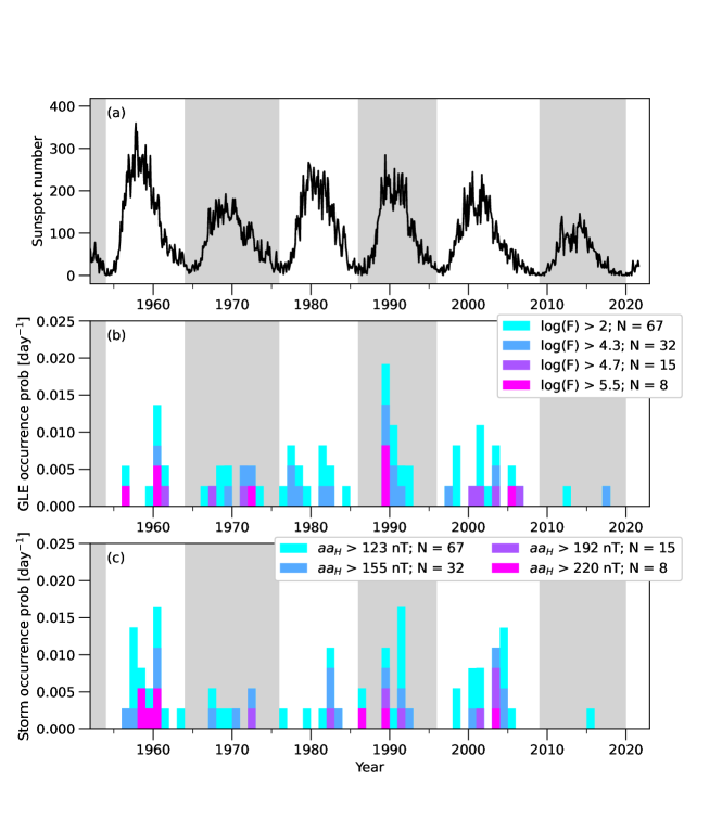
Figure 1.: Time series of (a) sunspot number, (b) GLE occurrence and (c) geomagnetic storm occurrence, as determined from the aa_H dataset. White/grey shaded regions show odd/even solar cycles, respectively.fig:timeseries

The first four recorded GLEs were measured using ionisation chambers (Forbush, 1946) and, as such, there are no estimates of event magnitude. The timing of GLEs during the neutron monitor era, from the 1950s onwards (Stoker, 2009), is provided by the GLE database https://gle.oulu.fi/) see Asvestari et al. (2017) for more detail. This database covers period from 1956 to early 2022 and includes 68 events. A number of smaller, ‘sub-GLE’, events have been identified in the more recent data (Miroshnichenko, Li, and Yanke, 2020), but these are not included in the present study so as to maintain a consistent event threshold throughout the 66-year interval considered. In order to estimate the GLE magnitude, we use the inferred spectral parameters to produce estimates of integrated fluence, $F$, above some rigidity threshold, $R$, using Equation 5 of Usoskin et al. (2020):

$$F(>R)=F_{0}\left(\frac{R}{1\,\textrm{GV}}\right)^{\gamma}\exp\left(\frac{-R}{R_{0}}\right)$$ (1)

where $F_{0}$ is a normalisation coefficient, $\gamma$ is the spectral index, and $R_{0}$ is the roll-off rigidity. Taking $R$ = 1 GV, and substituting for $J_{0}=4\pi F_{0}$, where $J_{0}$ is the integral intensity, this simplifies to:

$$F(>1\,\textrm{GV})=\frac{J_{0}}{4\pi}\exp\left(\frac{-1}{R_{0}}\right)$$ (2)

The spectral parameters $J_{0}$ and $R_{0}$ are provided by Usoskin et al. (2020) for 53 of the neutron-monitor era GLEs, giving $F(>1\,\textrm{GV})$ values in the range $2\times 10^{3}$ to $6\times 10^{6}$ cm^-2. For the remainder of the study, $F(>1\,\textrm{GV})$ [cm^-2] is simply referred to as $F$. The remaining 14 GLEs were deemed to be too small to enable reliable estimation of the spectrum. Here we use nominal values of $J_{0}=10^{4}$ and $R_{0}=\infty$, which results in $F=8\times 10^{2}$ cm^-2, to enable the timing of these small events – which is accurately known – to be included in the study. These data are provided as part of the supplementary material to this paper.

From this dataset, we produce a GLE-day time series for a range of $F$ thresholds. Including all the events (i.e. $\log(F)>2$) gives the full 67 events (one event is excluded, as described below). A threshold of $\log(F)>4.3$ approximately halves the number of events (32), while $\log(F)>4.7$ and $\log(F)>5.5$ give 15 and 8 events, respectively. The results presented here are not particularly sensitive to the choice of these thresholds, as can be verified using the provided code and data.

To compare GLEs with geomganetic storms, we use the aa_H index of geomagnetic activity (Lockwood et al., 2018b, a), averaged to 1 day. The aa_H index is based on the same data as the classical aa index but has been corrected to allow for secular change in the geomagnetic field and its effect on station response to space weather activity. In addition, calibrations between stations that allow for time-of-day and time-of-year have been employed which generates a much more homogeneous and accurate time series. Thresholds of aa_H are applied to select the days associated with the largest storms. Using daily aa_H thresholds of 123, 155, 192, and 220 nT gives 67, 32, 15, and 8 events, respectively, viz. the same statistics as for the GLEs. This enables direct comparison with the GLEs.

The monthly sunspot number, available from www.sidc.be/silso/datafiles, is used to determined the solar cycle phase and magnitude. The start and end of solar cycles are identified using the discontinuous change in the average latitude of the sunspots, as outlined in Owens et al. (2011). We further assume that Solar Cycle 25 began at the end of 2020. Using these solar-minimum times, the solar-cycle phase is computed as zero at the start of the cycle and increasing linearly to unity at the end. Thus not knowing the length of Cycle 25, we cannot compute the phase for the GLE 2021-10-28 and exclude it from the main study.

Figure fig:timeseries summarises these datasets. Panel a shows the monthly sunspot number, with the grey-shaded panels showing even-numbered solar cycles. Panel b shows the annual average occurrence probability of GLEs for the four $F$ thresholds. As all years contain complete data coverage, this is the number of events per year divided by the number of days in the year (i.e. 0.027 indicates one event in that year). Panel c shows the occurrence probability for geomagnetic storms, using aa_H thresholds chosen to give 67, 32, 15, and 8 events (i.e. the same number of total events as for GLEs at the four thresholds). From the time series alone, it is difficult to assess the degree to which GLEs follow the solar cycle or which GLE days correspond to geomagnetic storm days.

2.1 GLE Association with Extreme Geomagnetic Storms

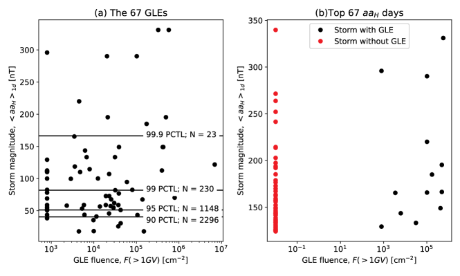
Figure 2.: The association between GLEs and geomagnetic storms (as measured by daily aa_H index). (a) The maximum aa_H within four days of each of the 67 GLEs as a function of GLE intensity. The black horizontal lines show percentile of aa_H over the whole 1956-2020 period. 32 of the 68 GLEs are associated with storms above the 99th percentile (which produces 230 storm days). (b) Black: The 13 of the top 67 aa_H days in the 1956-2020 period for which a GLE was present within four days. Red: The 54 of the top 67 storms for which no GLE was present. An intensity of 0.01 was assigned for plotting purposes.fig:aaH

Figure fig:aaHa shows the largest aa_H value within four days of the each GLE. There is no obvious correlation between GLE magnitude, as measured by $F$, and storm magnitude. More importantly, fewer than half the GLEs (32 of the 67) are associated with storms defined by the 99th percentile of aa_H, which produces 230 events in the period of study. The converse is shown in Figure fig:aaHb: The top 67 geomagnetic storm days as a function of GLE fluence within 4 days. For 54 of these top 67 storms, there was no GLE. Thus there is little event-by-event correlation between storms and GLEs (e.g. Nitta et al., 2012), and therefore we should not assume that the solar cycle trends found for geomagnetic storms apply to GLEs.

2.2 GLE occurrence over the solar cycle

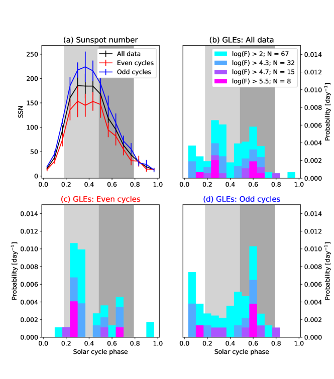
Figure 3.: Superposed epoch plots by solar cycle phase of (a) sunspot number and (b) GLE occurrence. Panels b and d show the GLE occurrence further divided in odd- and even-numbered solar cycles. Grey-shaded regions show the active phase of the solar cycle, identified with geomagnetic storms in Owens et al. (2021). Light and dark grey further divide the active phases into early and late active phases.fig:SPE

The time series shown in Figure fig:timeseries hint at GLE occurrence following the solar cycle and there does appear to be some evidence for larger cycles producing more GLEs, with the two smaller sunspot cycles peaking in 1970 and 2015 containing fewer GLEs than the four larger cycles. This is investigated statistically in Section sec:amp.

In order to better visualise the ordering (or otherwise) of GLEs as a function of the solar cycle, Figure fig:SPE shows a superposed epoch plot of GLE occurrence ordered by solar cycle phase. This normalises for variability in cycle length. For reference, grey-shaded panels show the active period identified for geomagnetic storms by Owens et al. (2021): The active phase starts at a phase of 0.18 and ends at a phase of 0.79. The light- and dark-grey shading bisects the early and late active period. It can be seen that GLEs of all magnitudes appear to be more common in the active period than the quiet period. The statistical significance of this result will be tested in Section sec:phase.

Figures fig:SPEc and d show the same analysis limited to even- and odd-numbered solar cycles, respectively. There is a prevalence of GLEs early in even-numbered cycles and late in odd-numbered cycles. Despite these GLEs being largely distinct events from extreme geomagnetic storms, they do appear to follow the same occurrence patterns: This same trend was reported for extreme geomagnetic storms (Owens et al., 2021) and has been seen in more quiescent geomagnetic activity (Cliver, Boriakoff, and Bounar, 1996) and solar wind conditions (Thomas, Owens, and Lockwood, 2013). Of course, by bisecting the dataset into odd and even cycles, the number of GLEs considered in each category is reduced by around a half. Thus it cannot be ruled out that this apparent ordering is purely by chance, rather than due to an underlying physical trend. This is investigated in Section sec:parity.

3 Probability Models

sec:models

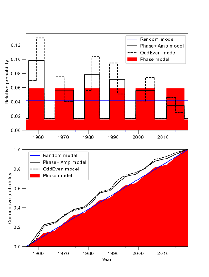
Figure 4.: Top: Models of GLE occurrence probability used to make inferences about the observations. Bottom: Cumulative distribution functions of the model probability, from which events are drawn. The Random model (blue) has a constant probability of a GLE at all times. The Phase model (red) has a factor four higher GLE probability during the active phase that the quiet phase. The Phase+Amp model further weights the active phase by the solar cycle amplitude (taken to be the cycle-average sunspot number). Finally, the OddEven model further adjusts the GLE occurrence probability up or down by a factor 0.3 during the early and late active phases based on the solar cycle parity (i.e. odd or even numbered).fig:models

Following the same approach as Owens et al. (2021), we test the apparent trends in GLE occurrence by comparing the observed occurrence with a number of different probability models. These are shown in the top panel of Figure fig:models. Details are discussed below, but briefly, the models are:

• Random model, shown by the solid blue line. In this model, the probability of GLE occurrence is equal at all times.

• Phase model, shown by the red shaded area. In this model, the probability of a GLE is a factor four higher during the active phase of the solar cycle (phase between 0.18 and 0.79) than during the quiet phase (all other times).

• Phase+Amp model, shown by the solid black line. This is the same as the Phase model, but the probability in the active phase of solar cycle $N$ is linearly related to the cycle amplitude, taken to be the average sunspot number over the cycle, $\langle SSN\rangle_{N}$.

• OddEven model, shown by the black dashed line. This is the Phase+Amp model, with a reduction in probability by a factor $(1+d)$ early in the active phase of odd cycles and late in even cycles, and an increase in probability by a factor $(1-d)$ in the late active phases of odd cycles and early in even cycles. We use $d=0.3$.

The coefficients in the Phase, Phase+Amp and OddEven models are chosen to approximately match the average values seen in Figure fig:SPE, though we do not attempt a ‘best fit’ of these values: the aim of the models is only to establish whether trends present in the data can or cannot be attributed to sampling issues. For the Phase+Amp and OddEven models, the probability in the active phase is further multiplied by a factor $\langle SSN\rangle_{N}/\langle SSN\rangle$, where $\langle SSN\rangle$ is the average SSN over the whole 1956 – 2021 interval, of 94.5.

From each probability model we construct the cumulative distribution functions, shown in the bottom panel of Figure fig:modelsb. From these, random events are drawn to produce time series of event occurrence consistent with the probability models.

4 Results

sec:results

4.1 Solar Cycle Phase

sec:phase

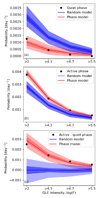
Figure 5.: GLE occurrence probability with increasing intensity threshold (a) in the quiet phase, (b) in the active phase, and (c) the difference between the active and quiet phases. Black circles show the observations. The blue lines, dark shaded and light-shaded areas show the median, one-sigma (i.e. 68%) and two-sigma (i.e. 95%) of 5000 Monte Carlo samplings of the Random model, wherein GLEs are assumed to have equal occurrence probability at all times. The red lines and shaded areas show the same for the Phase model, wherein GLEs are a factor four more probable in the active phase than in the quiet phase. fig:phase

We first test the significance of the apparent solar cycle phase trend in GLE occurrence. Specifically, we test the degree to which the observed difference in GLE occurrence probability in the quiet and active phases of the solar cycle can be explained purely by the random occurrence of a small number of events. Thus the Random model is our null hypothesis, as it assumes there is no underlying solar cycle trend. The Phase model, in which there is an underlying trend in the occurrence of GLEs with solar cycle phase, is the proposed hypothesis.

For each GLE intensity threshold (i.e. $\log(F)>2,4.3,4.7,5.5$ cm^-2), we produce a random time series of GLE occurrence consistent with the Random and Phase models, and containing the appropriate number of events (i.e. 67, 32, 15, and 8, respectively). For each model time series, we compute the average GLE occurrence probability in the quiet and active phase of the solar cycle. This is done 5,000 times to produce a Monte Carlo sampling of the average GLE occurrence probabilities in the quiet and active phases of the solar cycle.

Figure fig:phase shows the median, 1- and 2-sigma ranges (i.e. containing 68 and 95% of the samples) of the Monte Carlo samples of the model values. In the quiet phase (Figure fig:phasea), the Random model overestimates the observed occurrence probability for all GLE thresholds, while the Phase model is largely in agreement with the observations. Similarly, in the active phase (Figure fig:phaseb), the Random model underestimates the occurrence probability. These two trends are combined in Figure fig:phasec, which shows the difference between the active and quiet phase occurrence probability. The Random model is centred on zero, as expected. The observed values are well outside of 95% of the Random model values. Thus we can say that the Random model, in which there is no underlying solar cycle phase trend in GLE occurrence, is only consistent with the observations at a probability $p<0.05$. Conversely, the Phase model describes the observations well.

4.2 Solar Cycle Amplitude

sec:amp

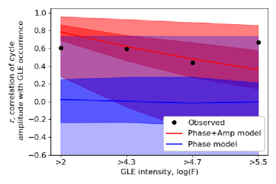
Figure 6.: The linear correlation, $r_{L}$, between solar cycle amplitude (as measured by the cycle-average sunspot number) and average GLE occurrence probability. Observations are shown by black circles. The blue lines, dark- and light-blue shaded areas show the median, one-sigma (i.e. 68%) and two-sigma (i.e. 95%) of 5000 Monte Carlo samplings of the Phase model, wherein GLEs are assumed to have equal occurrence probability in all cycles. The red lines and shaded areas show the same for the Phase+Amp model, wherein GLE occurrence probability increases linearly with cycle amplitude.fig:cyclemagnitude

The next test is to determine whether larger cycles produce more GLEs. For each GLE threshold, we compute the linear (or Pearson) correlation coefficient, $r_{L}$, between the cycle amplitude – as characterised by $SSN_{N}$ – and the average GLE occurrence probability over the cycle, $<p_{GLE}>_{N}$. For all thresholds, this correlation is based on only six data points (the six solar cycles in the dataset). However, if there is an underlying relation between $SSN_{N}$ and $<p_{GLE}>_{N}$, we might expect the correlation to drop with GLE threshold as $<p_{GLE}>_{N}$ becomes more poorly defined, being based on fewer events per cycle.

Figure fig:cyclemagnitude shows the observed correlation between $SSN_{N}$ and $<p_{GLE}>_{N}$ as a function of GLE intensity. The correlation remains reasonably constant at around $r_{L}=0.6$. At each threshold, $N=6$, thus using a Student t-test there is a reasonable probability ($p=0.2$) that the underlying correlation is zero and that this observed value occurred merely by chance. The Monte Carlo tests using the probability models reach a similar conclusion; while the observations agree more closely with the Phase+Amp model than the null hypothesis of the Phase model (wherein there is no relation between solar cycle amplitude and GLE occurrence), the null hypothesis still has a large probability ($p>0.05$) of describing the data.

4.3 Solar Cycle Parity

sec:parity

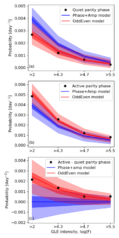
Figure 7.: GLE occurrence probability with increasing intensity threshold (a) in the quiet parity phases, i.e. early in even cycles, late in odd cycles, (b) in the active parity phases, i.e. late in even cycles, early in odd cycles, and (c) the difference between the active and quiet parity phases. Observations are shown in black. The blue line, dark shaded and light-shaded areas show the median, one-sigma (i.e. 68%) and two-sigma (i.e. 95%) of 5000 Monte Carlo samplings of the Phase+Amp model, wherein GLEs are assumed to have equal occurrence probability in the early and late active period. The red lines and shaded areas show the same for the OddEven model, wherein GLEs are a factor more probable in the early active phase in even cycles and in the late active phase in odd cycles. fig:oddeven

Next we test the apparent difference in GLE occurrence during solar cycles of different parity (i.e. even- and odd-numbered solar cycles). The Phase+Amp model serves as the null hypothesis, as it contains no difference between odd and even cycles. The proposed hypothesis – that there is an underlying preference for activity occurs earlier in even cycles and later in odd cycles – is tested using the OddEven model.

Figure fig:oddevena shows the average GLE occurrence probability in the combined quiet parity phases, i.e. late in the active phase of even cycles and early in the active phase of odd cycles. Figure fig:oddevena shows the same for the active parity phases (early in even cycles, later in odd cycles). The null hypothesis of no difference between odd and even cycles significantly overestimates GLE occurrence in the quiet parity phase at all GLE magnitudes, and systemically underestimates occurrence in the active phase (though cannot be ruled out at the 95% confidence level). The Phase+Amp model, on the other hand, is in general agreement. Figure fig:oddevenc shows the difference between these active and quiet parity phases. For the Phase+Amp model, the median value of the difference is zero, as expected, as there is no difference between odd and even cycles. It is clear that the observations are more consistent with the OddEven model. For three of the four GLE intensity thresholds considered, the observations are consistent with the null hypothesis with $p<0.05$.

4.4 GLE Waiting Times

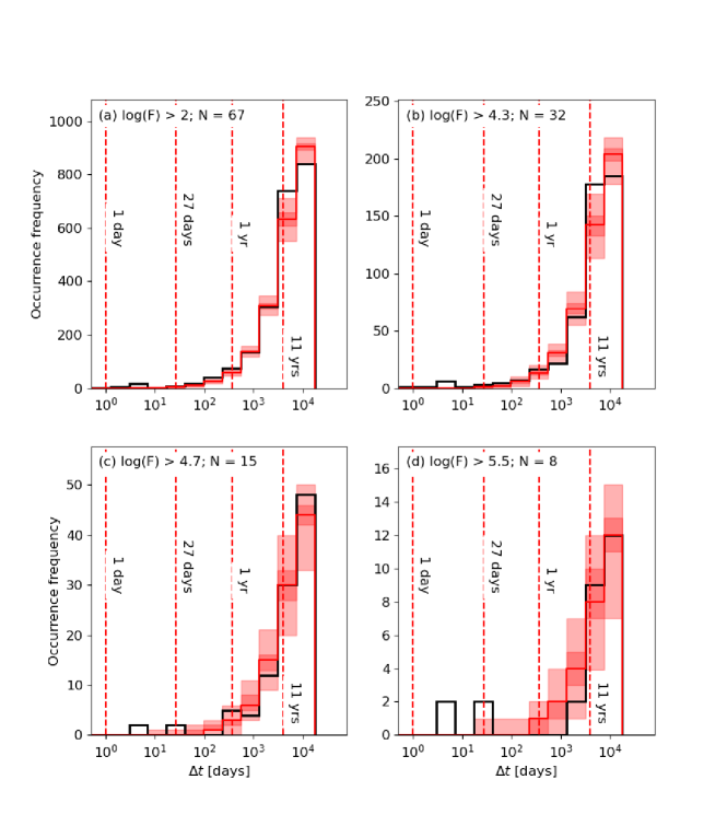
Figure 8.: Histograms of GLE waiting times for events defined by four different intensity thresholds. Note that the bins are equally spaced in log space. Red dashed vertical lines show a number of times of interest, for reference. Observations are shown in black. The red line, dark shaded and light-shaded areas show the median, one-sigma (i.e. 68%) and two-sigma (i.e. 95%) of Monte Carlo samples of the Random model. fig:waitingtimes

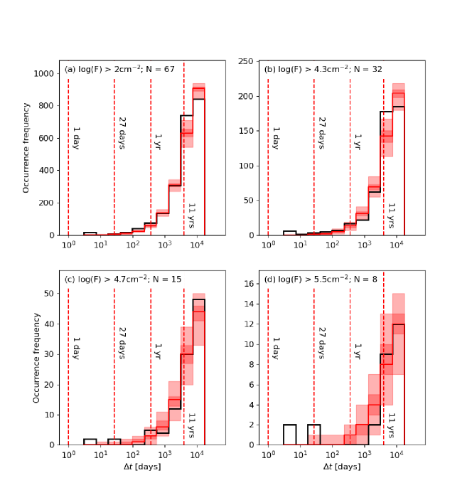
Figure 9.: Histograms of the separation times, $\Delta t$, between all possible GLE pairs for events defined by four different intensity thresholds. Note that the bins are equally spaced in log space. Red dashed vertical lines show a number of times of interest, for reference. Observations are shown in black. The red line, dark shaded and light-shaded areas show the median, one-sigma (i.e. 68%) and two-sigma (i.e. 95%) of Monte Carlo samples of the Random model. fig:dt

Some of the proposed Miyake events can require enhanced ¹⁴C production over multiple consecutive years (Sakurai et al., 2020). Given SEPs typically occur on the timescale of hours to days, multi-year ¹⁴C production requires clustering of extreme SEPs over a period of several months to years. Quasi-periodicities on these time scales have been reported for GLEs (Pérez-Peraza and Juárez-Zuñiga, 2015; Márquez-Adame, Pérez-Peraza, and Velasco-Herrera, 2019), though the statistics are dominated by the smaller magnitude events. We here examine the GLE record to assess the likelihood of such clustering of the most extreme events.

Figure fig:waitingtimes shows the waiting time between consecutive GLEs for different GLE amplitudes. The red shaded areas show the 1- and 2-sigma ranges of 5000 Monte Carlo samples of the Random model, i.e. containing 68 and 95% of the samples, respectively. Other models (Phase, Phase+Amp and OddEven) are not shown as they do not differ significantly from the Random model in that the events occur without correlation. At the lowest threshold shown in Figure fig:waitingtimesa, there are 16 events that occur within 10 days of a previous GLE. The clustering of these events are inconsistent with the random occurrence of events, and none of the other models considered in this study would produce such short-term clustering. This effect is likely multiple GLEs produced by a single, long-lived active region. Memory on these short time scales has been reported for lower intensity SEPs observed in near-Earth space (Jiggens and Gabriel, 2009), though CME and flare waiting times appear to follow a time-dependant Poisson process (Wheatland, 2003).

There is a large peak in events approximately 1 year after the previous GLE, but this is consistent with random occurrence of 67 events through the 60 year interval. This expected peak at approximately 1-year waiting time between consecutive GLEs persists out to $\log F>4.7$ cm^-2. For the higher thresholds there is not strong evidence for clustering at the 1-2 year timescale, but only 8 events are available for analysis. As GLE magnitude increases, the 11-year peak becomes more prominent, with GLEs being separated by a whole solar cycle, though the statistical significance is low.

Next, we look at the separation time between each possible GLE pair, $\Delta t$, shown in Figure fig:dt. In this dataset, $\Delta t$ can vary between the resolution of the data, at one day, and the length of the time series, approximately 60 years. As shown by comparison with the Monte Carlo sampling of the Random model, there is more clustering observed at very short times (less than a month) than would be expected. The solar cycle ordering of GLEs can be seen at lower event thresholds as a slight enhancement around $\Delta t=11$ yrs.

For both waiting time and $\Delta t$, we note some suggestion of a small peak around 27 days at all thresholds, suggesting some recurrent activity (though it could be associated with CMEs originating from the same active region, rather than necessarily from recurrent activity driven by corotating interaction regions).

5 Discussion

sec:discussion

In order to both better understand extreme space weather and to aid in the interpretation of ‘Miyake events’ in the cosmogenic-isotope records, this study has investigated solar cycle trends in the solar energetic particle (SEP) ground-level enhancement (GLE) record during the neutron monitor era. As there are only 67 events since 1956 (68 including the recent Solar Cycle 25 event), spanning only 6 solar cycles, it is necessary to carefully evaluate the probability that any apparent trends in GLE occurrence are not merely the result of random variations with a small sample size.

While such solar cycle trends were recently investigated for extreme geomagnetic storms, we show here that the one-to-one event association between GLEs and extreme geomagnetic storms is weak; most GLEs are not associated with a major geomagnetic storm and most major geomagnetic storms are not associated with a GLE. Thus solar cycle behaviour of storms should not be assumed a priori to apply to GLEs. The lack of a one-to-one event association is not surprising, as extreme storms require Earth-directed CMEs, whereas highest SEP fluence and hardest SEP spectra result from eruptions and shocks along the Earth-connected heliospheric magnetic flux tube (e.g. Reames, 1995). Owing to the Parker spiral configuration of the heliospheric magnetic field (Parker, 1958), this is nominally between 30 and 60 degrees West of Earth for coronal shocks. As the most SEP-productive shocks are fast and wide (Gopalswamy et al., 2008), the same shock and CME can be both directed along the Earth-connected HMF in the corona and encountered at Earth. However, for the most extreme storms it is likely the ‘nose’ of the shock (and thus typically the centre of the CME) that arrives at Earth. Similarly, for the most extreme SEPs, the nose of the shock likely threads the Earth-connected Parker spiral. Thus, the CMEs producing the highest SEP fluences at Earth are not Earth directed, and the most geoeffective CMEs are not directed along the Parker spiral-connected West limb of the Sun.

Despite the lack of association between events driving extreme storms and GLEs, the statistical behaviour of storm and GLE occurrence is remarkably similar. Thus GLEs act as independent sources of evidence of underlying solar-cycle trends in extreme solar activity reported by Owens et al. (2021). As with extreme geomagnetic storms, there is a clear solar cycle trend in GLE occurrence, with around a factor four increase in occurrence probability in an active period centred on solar maximum, compared with a quiet period centred on solar minimum. This trend is weaker in amplitude than reported for geomagnetic storms (Owens et al., 2021). Perhaps more surprisingly, GLEs also exhibit the 22-year trend for preferential occurrence earlier in even-numbered solar cycles and later in odd-numbered cycles. The most likely explanation for this trend is differing energetic particle drift patterns during opposing solar magnetic field polarities, which have long been known to affect GCR propagation through the heliosphere (Usoskin, 2017) and have recently been shown to have a significant effect on SEPs and GLEs (Waterfall et al., 2022). The relation between solar cycle amplitude and GLE occurrence cannot be conclusively measured, possibly owing to the few (six) solar cycles available for study. However, while the null hypothesis – of no relation – cannot be discounted, we note that: (a) the Phase+Amp model does describe the data better than the null hypothesis, and (b) extreme geomagnetic storm occurrence does exhibit a solar cycle amplitude trend (Owens et al., 2021), and GLEs follow the other two solar cycle trends in the same way as storms. Thus on balance, it seem more likely than not that larger solar cycles produce more GLEs.

There are a number of implications of these results for Miyake events (i.e., the spikes in the cosmogenic-isotope records). If Miyake events are more extreme GLEs, which are themselves extreme SEPs, then we might expect the same underlying patterns of occurrence. To assess if Miyake event follow the solar cycle phase trend requires multiple events, as it is inherently a statistical relation, and the probability difference between active and quiet phases is only around a factor four. It would also require precise determination of both the timing of the cosmogenic-isotope production enhancement and of the associated phase of the solar cycle. This would need to be within around 0.2 solar cycle phase, which is approximately 2 years. This may be difficult owing to the low signal-to-noise of the solar cycle in the ¹⁴C record, which often necessitates additional smoothing to identify (Brehm et al., 2021). On the other hand, ¹⁰Be in ice cores may have dating uncertainties of several years (e.g., Sukhodolov et al., 2017). The presence of a Miyake event further disturbs the underlying solar cycle signal, meaning phase must often be extrapolated from previous and subsequent cycles (Usoskin et al., 2021), adding uncertainty to the estimate. Even more difficult to assess from the ¹⁴C data is the change of behaviour between odd- and even-numbered solar cycles. The parity of the solar cycle cannot simply be tracked back from modern times due to breaks in cycle numbering through grand minima like the Maunder minimum. However, it has been shown that solar cycle parity can be reconstructed from the shape of the variation in ¹⁰Be data (Owens et al., 2015). Using similar measures it may be possible to infer cycle parity from ¹⁴C data and determine if the early/late behaviour is present for Miyake events.

Extreme SEPs are – by definition – rare. Therefore a physical explanation of ¹⁴C spikes that requires multiple extreme SEPs in a relatively short space of time becomes less probable, unless the occurrence of such events is expected to preferentially cluster in time over similar time scales. At lower GLE thresholds, a significant fraction of GLEs do occur within 1 year of previous events, though only at a rate consistent with random occurrence. As higher event thresholds are considered, times between GLEs shift to a more bimodal distribution of a few days, owing to multiple events produced by a single active region, and around 11 years, owing to the solar-cycle ordering of occurrence. These preferential time scales are too short and too long, respectively, to provide the required extended ¹⁴C production spike. Thus such Miyake events that can require multiple years of enhanced ¹⁴C production (e.g. circa 660 BCE; Sakurai et al., 2020) are less easy to explain in terms of solar-generated energetic particle events, if we think of them as the extreme event tail of the distribution to which the observed GLE events belong.

Acknowledgements

We have also benefited from sunspot data provided by Royal Observatory of Belgium SILSO and GLE data by the GLE database.

Funding

This work was part-funded by Science and Technology Facilities Council (STFC) grant numbers ST/R000921/1 and ST/V000497/1, and Natural Environment Research Council (NERC) grant numbers NE/S010033/1 and NE/P016928/1. I.U. acknowledges the Academy of Finland (projects ESPERA No. 321882). E.A. acknowledges support from the Academy of Finland (Postdoctoral Researcher Grant 322455), and the Finnish Centre of Excellence in Research of Sustainable Space (Academy of Finland grant number 312390).

Data Availability

Sunspot data are provided by the Royal Observatory of Belgium SILSO and available from www.sidc.be/silso/DATA/SN˙m˙tot˙V2.0.csv. The GLE database can be accessed here: https://gle.oulu.fi/. The aa_H-geomagnetic index data are available from www.swsc-journal.org/articles/swsc/olm/2018/01/swsc180022/swsc180022-2-olm.txt.

All analysis and visualisation code is packaged with all required OMNI data here: https://github.com/University-of-Reading-Space-Science/ExtremeEvents.

Declarations

Disclosure of Potential Conflict of Interest: We declare we have no conflicts of interest.

References

- Asvestari et al. (2017) Asvestari, E., Willamo, T., Gil, A., Usoskin, I.G., Kovaltsov, G.A., Mikhailov, V.V., Mayorov, A.: 2017, Analysis of Ground Level Enhancements (GLE): Extreme solar energetic particle events have hard spectra. Adv. Space Res. 60, 781. DOI.
- Barnard and Lockwood (2011) Barnard, L., Lockwood, M.: 2011, A survey of gradual solar energetic particle events. J. Geophys. Res. 116, A05103. DOI.
- Barnard et al. (2018) Barnard, L., McCracken, K.G., Owens, M.J., Lockwood, M.: 2018, What can the annual 10Be solar activity reconstructions tell us about historic space weather? J. Space Weather and Space Climate 8, A23. DOI.
- Brehm et al. (2021) Brehm, N., Bayliss, A., Christl, M., Synal, H.-A., Adolphi, F., Beer, J., Kromer, B., Muscheler, R., Solanki, S.K., Usoskin, I., Bleicher, N., Bollhalder, S., Tyers, C., Wacker, L.: 2021, Eleven-year solar cycles over the last millennium revealed by radiocarbon in tree rings. Nat. Geosci. 14, 10. DOI.
- Caballero-Lopez et al. (2004) Caballero-Lopez, R.A., Moraal, H., McCracken, K.G., McDonald, F.B.: 2004, The heliospheric magnetic field from 850 to 2000 AD inferred from 10Be records. J. Geophys. Res. 109, 12102. DOI.
- Chapman et al. (2020) Chapman, S.C., McIntosh, S.W., Leamon, R.J., Watkins, N.W.: 2020, Quantifying the Solar Cycle Modulation of Extreme Space Weather. Geophys. Res. Lett. 47, e2020GL087795. DOI.
- Clette and Lefèvre (2016) Clette, F., Lefèvre, L.: 2016, The new sunspot number: assembling all corrections. Solar Phys. 291, 2629. DOI.
- Cliver (1994) Cliver, E.W.: 1994, Solar activity and geomagnetic storms: The first 40 years. EOS Transactions 75, 569.
- Cliver, Boriakoff, and Bounar (1996) Cliver, E.W., Boriakoff, V., Bounar, K.H.: 1996, The 22‐year cycle of geomagnetic and solar wind activity. J. Geophys. Res. 101, 27091.
- Cliver et al. (2014) Cliver, E.W., Tylka, A.J., Dietrich, W.F., Ling, A.G.: 2014, On a Solar Origin for the Cosmogenic Nuclide Eevent of 775 A.D. Astrophys. J. 781, 32. DOI.
- Cliver et al. (2020) Cliver, E.W., Hayakawa, H., Love, J.J., Neidig, D.F.: 2020, On the Size of the Flare Associated with the Solar Proton Event in 774 AD. Astrophys. J. 903, 41. DOI.
- Cliver et al. (2022) Cliver, E.W., Schrijver, C.J., Shibata, K., Usoskin, I.G.: 2022, Extreme solar events. Living Rev. Sol. Phys. 19, 2. DOI.
- Dee et al. (2017) Dee, M., Pope, B., Miles, D., Manning, S., Miyake, F.: 2017, Supernovae and Single-Year Anomalies in the Atmospheric Radiocarbon Record. Radiocarbon 59, 293. DOI.
- Desai and Giacalone (2016) Desai, M., Giacalone, J.: 2016, Large gradual solar energetic particle events. Living Rev. Sol. Phys. 13, 3. DOI.
- Forbush (1946) Forbush, S.E.: 1946, Three Unusual Cosmic-Ray Increases Possibly Due to Charged Particles from the Sun. Phys. Rev. 70, 771. Publisher: American Physical Society. DOI.
- Gopalswamy et al. (2008) Gopalswamy, N., Yashiro, S., Akiyama, S., Mäkelä, P., Xie, H., Kaiser, M.L., Howard, R.A., Bougeret, J.L.: 2008, Coronal mass ejections, type II radio bursts, and solar energetic particle events in the SOHO era. Ann. Geophys. 26, 3033. DOI.
- Gosling (1993) Gosling, J.T.: 1993, The solar flare myth. J. Geophys. Res. 98, 18937. DOI.
- Hambaryan and Neuhäuser (2013) Hambaryan, V.V., Neuhäuser, R.: 2013, A Galactic short gamma-ray burst as cause for the 14C peak in AD 774/5. Mon. Not. Roy. Astron. Soc. 430, 32. DOI.
- Hudson (2021) Hudson, H.S.: 2021, Carrington Events. Annu. Rev. Astron. Astrophys. 59, 445. DOI.
- Jiggens and Gabriel (2009) Jiggens, P.T.A., Gabriel, S.B.: 2009, Time distributions of solar energetic particle events: Are SEPEs really random? J. Geophys. Res. 114. DOI.
- Kilpua et al. (2015) Kilpua, E.K.J., Olspert, N., Grigorievskiy, A., Käpylä, M.J., Tanskanen, E.I., Miyahara, H., Kataoka, R., Pelt, J., Liu, Y.D.: 2015, Statistical Study of Strong and Extreme Geomagnetic Disturbances and Solar Cycle Characteristics. Astrophys. J. 806, 272. DOI.
- Liu et al. (2014) Liu, Y., Zhang, Z.-f., Peng, Z.-c., Ling, M.-x., Shen, C.-C., Liu, W.-g., Sun, X.-c., Shen, C.-d., Liu, K.-x., Sun, W.: 2014, Mysterious abrupt carbon-14 increase in coral contributed by a comet. Scientific Reports 4, 3728. DOI.
- Lockwood et al. (2013) Lockwood, M., Barnard, L., Nevanlinna, H., Owens, M.J., Harrison, R.G., Rouillard, A.P., Davis, C.J.: 2013, Reconstruction of geomagnetic activity and near-Earth interplanetary conditions over the past 167 yr - Part 1: A new geomagnetic data composite. Ann. Geophys. 31, 1957. DOI.
- Lockwood et al. (2018a) Lockwood, M., Chambodut, A., Barnard, L.A., Owens, M.J., Clarke, E., Mendel, V.: 2018a, A homogeneous aa index: 1. Secular variation. J. Space Weather Space Clim. 8, A53. DOI.
- Lockwood et al. (2018b) Lockwood, M., Finch, I.D., Chambodut, A., Barnard, L.A., Owens, M.J., Clarke, E.: 2018b, A homogeneous aa index: 2. Hemispheric asymmetries and the equinoctial variation. J. Space Weather Space Clim. 8, A58. DOI.
- Low (2001) Low, B.C.: 2001, Coronal mass ejections, magnetic flux ropes, and solar magnetism. J. Geophys. Res. 106, 25141. DOI.
- Lynch et al. (2005) Lynch, B.J., Gruesbeck, J.R., Zurbuchen, T.H., Antiochos, S.K.: 2005, Solar cycle dependent helicity transport by magnetic clouds. J. Geophys. Res. 110, A08107. DOI.
- Melott and Thomas (2012) Melott, A.L., Thomas, B.C.: 2012, Causes of an AD 774–775 14C increase. Nature 491, E1. DOI.
- Miroshnichenko (2018) Miroshnichenko, L.I.: 2018, Retrospective analysis of GLEs and estimates of radiation risks. J. Space Weather and Space Climate 8, A52. DOI.
- Miroshnichenko, Li, and Yanke (2020) Miroshnichenko, L.I., Li, C., Yanke, V.G.: 2020, Small Size Ground Level Enhancements During Solar Cycle 24. Solar Phys. 295, 102. DOI.
- Miyake, Masuda, and Nakamura (2013) Miyake, F., Masuda, K., Nakamura, T.: 2013, Another rapid event in the carbon-14 content of tree rings. Nat. Commun. 4, 1748. DOI.
- Miyake et al. (2012) Miyake, F., Nagaya, K., Masuda, K., Nakamura, T.: 2012, A signature of cosmic-ray increase in AD 774–775 from tree rings in Japan. Nature 486, 240. DOI.
- Mursula, Usoskin, and Maris (2007) Mursula, K., Usoskin, I.G., Maris, G.: 2007, Introduction to Space Climate. Adv. Space Res. 40, 885. DOI.
- Márquez-Adame, Pérez-Peraza, and Velasco-Herrera (2019) Márquez-Adame, J.C., Pérez-Peraza, J., Velasco-Herrera, V.: 2019, Determination of GLE of Solar Energetic Particles by Means of Spectral Analysis. Astrophys. J. 878, 154. DOI.
- Nandy (2021) Nandy, D.: 2021, Progress in Solar Cycle Predictions: Sunspot Cycles 24–25 in Perspective. Solar Phys. 296, 54. DOI.
- Nitta et al. (2012) Nitta, N.V., Liu, Y., DeRosa, M.L., Nightingale, R.W.: 2012, What Are Special About Ground-Level Events? Space Sci. Rev. 171, 61. DOI.
- Notsu et al. (2019) Notsu, Y., Maehara, H., Honda, S., Hawley, S.L., Davenport, J.R.A., Namekata, K., Notsu, S., Ikuta, K., Nogami, D., Shibata, K.: 2019, Do Kepler Superflare Stars Really Include Slowly Rotating Sun-like Stars? - Results Using APO 3.5 m Telescope Spectroscopic Observations and Gaia-DR2 Data. Astrophys. J. 876, 58. DOI.
- Okamoto et al. (2021) Okamoto, S., Notsu, Y., Maehara, H., Namekata, K., Honda, S., Ikuta, K., Nogami, D., Shibata, K.: 2021, Statistical Properties of Superflares on Solar-type Stars: Results Using All of the Kepler Primary Mission Data. Astrophys. J. 906, 72. DOI.
- Owens and Crooker (2006) Owens, M.J., Crooker, N.U.: 2006, Coronal mass ejections and magnetic flux buildup in the heliosphere. J. Geophys. Res. 111, A10104. DOI.
- Owens et al. (2011) Owens, M.J., Lockwood, M., Barnard, L., Davis, C.J.: 2011, Solar cycle 24: implications for energetic particles and long-term space climate change. Geophys. Res. Lett. 38, 1. DOI.
- Owens et al. (2015) Owens, M.J., McCracken, K.G., Lockwood, M., Barnard, L.: 2015, The heliospheric Hale cycle over the last 300 years and its implications for a “lost” late 18th century solar cycle. J. Space Weather and Space Clim. 5, A30. DOI.
- Owens et al. (2016a) Owens, M.J., Cliver, E.W., McCracken, K.G., Beer, J., Balogh, A., Barnard, L., Lockwood, M., Rouillard, A.P., Wang, Y.-M., Passos, S., Riley, P., Usoskin, I.: 2016a, Near-Earth Heliospheric Magnetic Field Intensity Since 1750. Part 1: Sunspot and Geomagnetic Reconstructions. J. Geophys. Res. 121, 6048. DOI.
- Owens et al. (2016b) Owens, M.J., Cliver, E.W., McCracken, K.G., Beer, J., Balogh, A., Barnard, L., Lockwood, M., Rouillard, A.P., Wang, Y.-M., Passos, S., Riley, P., Usoskin, I.: 2016b, Near-Earth Heliospheric Magnetic Field Intensity Since 1750. Part 2: Cosmogenic Radionuclide Reconstructions. J. Geophys. Res. 121, 6064. DOI.
- Owens et al. (2021) Owens, M.J., Lockwood, M., Barnard, L.A., Scott, C.J., Haines, C., Macneil, A.: 2021, Extreme Space-Weather Events and the Solar Cycle. Solar Phys. 296, 82. DOI.
- Parker (1958) Parker, E.N.: 1958, Dynamics of the interplanetary gas and magnetic fields. Astrophys. J. 128, 664. DOI.
- Pesnell (2020) Pesnell, W.D.: 2020, Lessons learned from predictions of Solar Cycle 24. J. Space Weather Space Clim. 10, 60. DOI.
- Pérez-Peraza and Juárez-Zuñiga (2015) Pérez-Peraza, J., Juárez-Zuñiga, A.: 2015, Prognosis of GLEs of Relativistic Solar Protons. Astrophys. J. 803, 27. DOI.
- Reames (1995) Reames, D.V.: 1995, Solar energetic particles: A paradigm shift. Rev. Geophys. 33, 585.
- Reames (2013) Reames, D.V.: 2013, The Two Sources of Solar Energetic Particles. Space Sci. Rev. 175, 53. DOI.
- Richardson and Cane (2010) Richardson, I.G., Cane, H.V.: 2010, Near-Earth Interplanetary Coronal Mass Ejections During Solar Cycle 23 (1996 – 2009): Catalog and Summary of Properties. Solar Phys. 264, 189. DOI.
- Richardson, Cane, and Cliver (2002) Richardson, I.G., Cane, H.V., Cliver, E.W.: 2002, Sources of geomagnetic activity during nearly three solar cycles (1972-2000). J. Geophys. Res. 107. DOI.
- Sakurai et al. (2020) Sakurai, H., Tokanai, F., Miyake, F., Horiuchi, K., Masuda, K., Miyahara, H., Ohyama, M., Sakamoto, M., Mitsutani, T., Moriya, T.: 2020, Prolonged production of 14C during the ~660 BCE solar proton event from Japanese tree rings. Scientific Reports 10, 660. DOI.
- Shea and Smart (1990) Shea, M.A., Smart, D.F.: 1990, A summary of major solar proton events. Solar Phys. 127, 297. DOI.
- Solanki et al. (2004) Solanki, S.K., Usoskin, I.G., Kromer, B., Schüssler, M., Beer, J.: 2004, Unusual activity of the Sun during recent decades compared to the previous 11,000 years. Nature 431, 1084. DOI.
- Steinhilber et al. (2012) Steinhilber, F., Abreu, J.A., Beer, J., Brunner, I., Christl, M., Fischer, H., Heikkila, U., Kubik, P.W., Mann, M., McCracken, K.G., Miller, H., Miyahara, H., Oerter, H., Wilhelms, F.: 2012, 9,400 years of cosmic radiation and solar activity from ice cores and tree rings. Proc. Natl. Acad. Sci. 109, 5967. DOI.
- Stoker (2009) Stoker, P.H.: 2009, The IGY and beyond: A brief history of ground-based cosmic-ray detectors. Adv. Space Res. 44, 1081. DOI.
- Sukhodolov et al. (2017) Sukhodolov, T., Usoskin, I., Rozanov, E., Asvestari, E., Ball, W.T., Curran, M.A.J., Fischer, H., Kovaltsov, G., Miyake, F., Peter, T., Plummer, C., Schmutz, W., Severi, M., Traversi, R.: 2017, Atmospheric impacts of the strongest known solar particle storm of 775 AD. Scientific Reports 7, 45257. DOI.
- Svalgaard and Cliver (2005) Svalgaard, L., Cliver, E.W.: 2005, The IDV index: Its derivation and use in inferring long-term variations of the interplanetary magnetic field strength. J. Geophys. Res. 110, 12103. DOI.
- Thomas, Owens, and Lockwood (2013) Thomas, S.R., Owens, M.J., Lockwood, M.: 2013, The 22-Year Hale Cycle in Cosmic Ray Flux - Evidence for Direct Heliospheric Modulation. Solar Phys. 289, 407. DOI.
- Usoskin (2017) Usoskin, I.G.: 2017, A History of Solar Activity over Millennia. Liv. Rev. Sol. Phys. 14. DOI.
- Usoskin and Kovaltsov (2015) Usoskin, I.G., Kovaltsov, G.A.: 2015, The carbon-14 spike in the 8th century was not caused by a cometary impact on Earth. Icarus 260, 475. DOI.
- Usoskin et al. (2013) Usoskin, I.G., Kromer, B., Ludlow, F., Beer, J., Friedrich, M., Kovaltsov, G.A., Solanki, S.K., Wacker, L.: 2013, The AD775 cosmic event revisited: the Sun is to blame. Astron. Astrophys. 552, L3. DOI.
- Usoskin et al. (2021) Usoskin, I.G., Solanki, S.K., Krivova, N.A., Hofer, B., Kovaltsov, G.A., Wacker, L., Brehm, N., Kromer, B.: 2021, Solar cyclic activity over the last millennium reconstructed from annual 14C data. Astron. Astrophys. 649, A141. DOI.
- Usoskin et al. (2020) Usoskin, I., Koldobskiy, S., Kovaltsov, G.A., Gil, A., Usoskina, I., Willamo, T., Ibragimov, A.: 2020, Revised GLE database: Fluences of solar energetic particles as measured by the neutron-monitor network since 1956. Astron. Astrophys. 640, A17. DOI.
- van Driel-Gesztelyi and Owens (2020) van Driel-Gesztelyi, L., Owens, M.J.: 2020, Solar Cycle, Oxford University Press, Oxford, UK. DOI.
- Vennerstrom et al. (2016) Vennerstrom, S., Lefevre, L., Dumbovic, M., Crosby, N., Malandraki, O., Patsou, I., Clette, F., Veronig, A., Vrsnak, B., Leer, K., Moretto, T.: 2016, Extreme Geomagnetic Storms - 1868 - 2010. Solar Phys. 291, 1447 . DOI.
- Wang et al. (2019) Wang, F.Y., Li, X., Chernyshov, D.O., Hui, C.Y., Zhang, G.Q., Cheng, K.S.: 2019, Consequences of Energetic Magnetar-like Outbursts of Nearby Neutron Stars: 14C Events and the Cosmic Electron Spectrum. Astrophys. J. 887, 202. DOI.
- Waterfall et al. (2022) Waterfall, C.O.G., Dalla, S., Laitinen, T., Hutchinson, A., Marsh, M.: 2022, Modelling the transport of relativistic solar protons along a heliospheric current sheet during historic GLE events. Astrophys. J. in press. arXiv:2206.11650 [astro-ph, physics:physics]. DOI.
- Wheatland (2003) Wheatland, M.S.: 2003, The Coronal Mass Ejection Waiting-Time Distribution. Solar Phys. 214, 361. DOI.