The K2-3 system revisited: testing photoevaporation and core-powered mass loss with three small planets spanning the radius valley

Abstract

Multi-planet systems orbiting M dwarfs provide valuable tests of theories of small planet formation and evolution. K2-3 is an early M dwarf hosting three small exoplanets (1.5–2.0 R_⊕) at distances of 0.07–0.20 AU. We measure the high-energy spectrum of K2-3 with HST/COS and XMM-Newton, and use empirically-driven estimates of Ly-$\alpha$ and extreme ultraviolet flux. We use EXOFASTv2 to jointly fit radial velocity, transit, and SED data. This constrains the K2-3 planet radii to 4% uncertainty and the masses of K2-3b and c to 13% and 30%, respectively; K2-3d is not detected in RV measurements. K2-3b and c are consistent with rocky cores surrounded by solar composition envelopes (mass fractions of $0.36^{+0.14}_{-0.11}\%$ and $0.07^{+0.09}_{-0.05}\%$), H₂O envelopes ($55^{+14}_{-12}\%$ and $16^{+17}_{-10}\%$), or a mixture of both. However, based on the high-energy output and estimated age of K2-3, it is unlikely that K2-3b and c retain solar composition atmospheres. We pass the planet parameters and high-energy stellar spectrum to atmospheric models. Dialing the high-energy spectrum up and down by a factor of 10 produces significant changes in trace molecule abundances, but not at a level detectable with transmission spectroscopy. Though the K2-3 planets span the small planet radius valley, the observed system architecture cannot be readily explained by photoevaporation or core-powered mass loss. We instead propose 1) the K2-3 planets are all volatile-rich, with K2-3d having a lower density than typical of super-Earths, and/or 2) the K2-3 planet architecture results from more stochastic processes such as planet formation, planet migration, and impact erosion.

1 Introduction

Small exoplanets are currently divided into two broad categories: those smaller than about 1.7 R_⊕ are dubbed super-Earths and are considered to be terrestrial in nature, with iron-silicate ratios similar to those of Earth and Venus, while those with radii between 1.7 and about 4 R_⊕ have bulk densities consistent with degenerate amounts of iron, rock, ice and volatiles. The exoplanets in the second category are referred to as sub-Neptunes or gas dwarfs, given that their compositions must include some amount of low mean molecular weight material (hydrogen and helium) in order to explain their bulk densities. An extended hydrogen/helium atmosphere can make up only a few percent of a sub-Neptune’s mass but contribute half of its observed radius (Owen et al., 2020). Though we can measure the radii and masses of super-Earths and sub-Neptunes, these values can only provide a bulk density; we do not know the compositions of these worlds a priori. There is a well-measured valley in the radius distribution that separates the super-Earths and sub-Neptunes (Fulton et al., 2017; Fulton & Petigura, 2018; Van Eylen et al., 2018; Martinez et al., 2019), but the nature of the valley is not consistent across stellar types.

For FGK stars there is a slope in the radius valley that trends towards larger planet radii with increasing instellation (or decreasing orbital period; Fulton et al., 2017; Van Eylen et al., 2018; Martinez et al., 2019). This change in location of the radius valley as a function of instellation gives rise to the narrative that small planets start out with hydrogen/helium envelopes but experience subsequent atmosphere sculpting. This can be explained by photoevaporation driven by the host star (Owen & Wu, 2013; Lopez & Fortney, 2013) and/or core-powered mass loss driven by energy left over from planetary formation (Ginzburg et al., 2016, 2018; Gupta & Schlichting, 2019).

On the other hand, low-mass stellar systems with $T_{\mathrm{eff}}<4700$ K observed by the Kepler and K2 missions show a tentative shallow trend in the radius valley towards larger planet radii with decreasing instellation (increasing orbital period; Cloutier & Menou, 2020). This trend might be better explained by different formation timescales for sub-Neptunes and super-Earths: sub-Neptune worlds form rapidly ($<10$ Myr) and are able to accrete hydrogen and helium from the proto-planetary gas disc, while super-Earths take longer ($>10$ Myr) to form and do not have time to accrete gas from the disc before it dissipates (Lopez & Rice, 2018). However, gas remaining in the outer disc while the inner disc is depleted can seep into the inner disc while the terrestrial cores are forming (gas-poor formation), in which case the trend in the radius valley again resembles what is observed generally for FGK stars (Lee & Connors, 2021). It should be noted that with a temperature cut-off of 4700 K, the low-mass stellar sample includes both M and K dwarfs, and that the sample of planets is an order of magnitude smaller than that of FGK planets, so the planet radius valley for low-mass stars and its trend towards decreasing instellation is not definitive (Cloutier & Menou, 2020).

Multi-planet systems allow for comparative planetology in the presence of a common star. The high-energy radiation from the stellar host can be factored out of the equation, so the different atmospheric outcomes of the planets are dependent only on their orbital distance. This is particularly powerful when we are unsure of the high-energy history of the stellar host, as is the case for most M dwarfs. M dwarfs are known to exhibit longer periods of activity in the pre-main sequence phase when compared to Sun-like stars and it is difficult to determine their ages, which would help to constrain the total amount of high-energy radiation an M dwarf planet experiences in its lifetime so far. In light of the difficulties presented by M dwarfs as small planet hosts, assessing the system architectures and planetary atmospheres of multi-planet M dwarf systems can provide evidence for the various theories of planet formation and evolution in the presence of these low-mass stars.

Here we take a deep dive into the K2-3 system. K2-3 is an early M dwarf ($M=0.55\mathrm{M}_{\odot}$, $T_{\mathrm{eff}}=3844\mathrm{K}$, $K_{s}=8.561$) hosting three small exoplanets (Crossfield et al., 2015). An early find by the K2 mission (Howell et al., 2014), this system is the subject of several follow-up observations to constrain the radii and masses of K2-3b, c, and d. Transit observations from K2 (Crossfield et al., 2015) and Spitzer (GO Program 11026, PI Werner; GO Program 12081, PI Benneke; Kosiarek et al., 2019) constrain the radii of the K2-3 worlds, while radial velocity measurements from ESO La Silla/HARPS (Almenara et al., 2015), Magellan II/PFS (Dai et al., 2016), TNG/HARPS-N (Damasso et al., 2018), and Keck I/HIRES (Kosiarek et al., 2019) constrain their masses. K2-3b, the inner-most planet, has a radius and mass consistent with a sub-Neptune world. K2-3c, the middle planet, has a composition closer to terrestrial but has a slightly lower mass that points to the presence of extra volatiles. K2-3d, the outer-most world is not detected in the RVs but its radius of 1.5 R_⊕ is consistent with what is expected for a terrestrial type world (e.g., Rogers, 2015; Chen & Kipping, 2017; Kanodia et al., 2019). K2-3d also happens to orbit at the inner edge of the system’s habitable zone (Kopparapu et al., 2014).

In this work we present the high-energy spectrum of the host star K2-3 and refine the planet parameters using a joint fit between transit, radial velocity, and SED measurements. We do not have measurements of the K2-3 planetary atmospheres so instead we test a range of atmospheres for each planet in the presence of the high-energy stellar spectrum in order to determine a possible range of atmospheric outcomes for these worlds. We include the effects of disequilibrium chemistry in these models, which is appropriate for worlds smaller and cooler than hot Jupiters, which can generally be assumed to be in thermal equilibrium.

In Section 2 we describe the observations, analysis, and resulting data products of the high energy spectrum of the star K2-3. In Section 3 we discuss the global fit that results in the planetary parameters used in this work. In Section 4 we combine our knowledge of the stellar spectrum with interior and atmospheric models of the K2-3 planets. We present a discussion of this work and its implications for the observed K2-3 system architecture in Section 5. Concluding remarks can be found in Section 6.

The panchromatic spectrum of K2-3 in various forms can be found as a MAST high level science product at doi: 10.17909/t9-fqky-7k61 (catalog 10.17909/t9-fqky-7k61) (details in Section 2).

Table 1: Observations of K2-3 with HST/COS

Visit	Orbit	Grating	Central Wavelength	Wavelength Range	Resolution Rangea	Exposure Time	FP-POSb
			(Å)	(Å)	($\times 10^{3}$)	(s)
	1	G230L	2950	1677–3215	2.1–3.9	4 $\times$ 60	1,2,3,4
	1					706	3
	2	G130M	1291	1132–1430	12–16	2915	4
1	3					1682	3
	3					996	1
	4	G160M	1589	1395–1766	13–20	2915	2
	5					2915	3
	6					2915	4

Note. — At the time these data were taken (14 November 2017) the G130M and G160M gratings were placed at lifetime position four (LP4) on the FUV detector to mitigate gain sag and extend the detector lifetime.

^a Resolving power $R=\lambda/\mathrm{FWHM}$ from Table 5.1 of the COS Instrument Handbook v13

^b Changing the fixed-pattern position (FP-POS) shifts the spectrum slightly in the dispersion direction such that spectral features fall on different detector pixels. This is done to overcome limitations in S/N achievable with each grating due to fixed-pattern noise in the COS detectors.

2 Panchromatic Spectrum of K2-3

To construct the panchromatic spectrum of K2-3 we must combine information from multiple sources, including observations, estimates, and models. In this section we break down each piece of the spectrum and explain how we arrived at the flux density before putting it all together in a spectrum that spans 1–10⁵ Å.

2.1 Ultraviolet

We observed K2-3 in both the far-UV (FUV=912–1700Å) and near-UV (NUV=1700-3200Å) with the Cosmic Origins Spectrograph on board the Hubble Space Telescope (HST/COS). We observed for six orbits in a single visit on 14 November 2017 to obtain these data (GO Program 15110, PI L. Kreidberg). Details of the observations, including the grating, wavelength range, and exposure times can be found in Table 1. The HST/COS pipeline combines observations taken with the same grating and provides wavelength-calibrated 1D spectra for each grating. A resolution element of the COS FUV detector spans $6\times 10$ pixels and for the COS NUV detector $3\times 3$ pixels (COS Instrument Handbook v13 Chapter 3.2). We bin the 1D spectra in each grating by 4 pixels per bin for gratings G130M and G160M and by 3 pixels for G230L. We then combine the spectra from the three gratings and Doppler shift the spectrum in wavelength space according to the systemic radial velocity of K2-3 (30.76 km/s; Gaia Collaboration et al., 2018).

2.1.1 Ly-$\alpha$

As part of the design philosophy for COS to achieve high throughput of point sources in the FUV, COS is effectively a slitless spectrograph with a large entrance aperture (2.5^′′ diameter) (Green et al., 2012). As a result, COS spectra suffer from significant geocoronal contamination originating in Earth’s atmosphere at the N i (1200Å) Ly$\alpha$ (1214Å), and O i (1302, 1305, 1306Å) lines. We assume that measured N i and O i flux is entirely contaminated and we set the flux density in the narrow ranges around these lines (1198–1202Å, 1301–1308Å, and 1354–1357Å) to 0 erg cm^-2 s^-1 Å^-1. The Ly$\alpha$ flux makes up 85% of M dwarf FUV flux (France et al., 2016) so it cannot be zeroed out without significantly affecting our understanding of the UV spectrum. In the case of some M dwarf observations in the UV it is possible to observe the red and blue wings of the Ly$\alpha$ line using HST/STIS, which has a narrower slit and therefore experiences less geocoronal contamination (France et al., 2016). However, the Ly$\alpha$ line core is still inaccessible due to absorption by neutral hydrogen in the interstellar medium. The Ly$\alpha$ line wing observations by HST/STIS allow for a reconstruction of the Ly$\alpha$ line (Youngblood et al., 2016), but such observations become prohibitively expensive for inactive mid-M dwarfs beyond $\sim$15 pc. For K2-3 we instead use the UV lines that we do measure in the FUV and NUV along with known UV-UV flux correlations (Youngblood et al., 2017) to estimate K2-3’s Ly$\alpha$ line flux.

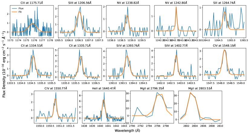
Figure 1: Measured transition region lines (blue) listed in Table 2, with subplots for each transition. The transition lines are fitted with Gaussian functions convolved with COS LSFs (orange).

Similar to the procedure laid out in Diamond-Lowe et al. (2021), we fit the observed UV lines with Gaussian profiles convolved with the appropriate COS line spread function (Figure 1) and then integrate under the resulting curve to determine the line flux. We scale these apparent fluxes by the distance and radius of K2-3 to get their surface fluxes (Table 2). To estimate the surface flux of Ly$\alpha$ we use the measured surface fluxes along with the UV-UV correlation equations which take the form

$$\mathrm{log}_{10}(F_{\mathrm{Surf},\mathrm{UV_{1}}})=m\times\mathrm{log}_{10}(F_{\mathrm{Surf},\mathrm{UV_{2}}})+b$$ (1)

where $F_{\mathrm{Surf},\mathrm{UV_{1}}}$ is the Ly$\alpha$ surface flux we want to estimate, $F_{\mathrm{Surf},\mathrm{UV_{2}}}$ is the surface flux of one of the measured transition region lines, $m$ is the fitted slope of the correlation between line 1 and line 2, and $b$ is the fitted $y$-intercept of the correlation. The variables $m$ and $b$ are provided in Table 9 of Youngblood et al. (2017) for the transition lines listed in Table 2. Our resulting estimates for K2-3’s Ly$\alpha$ flux from each measured line are provided in Table 3.

To determine the uncertainties in the Ly$\alpha$ estimate from each measured emission line we account for both the uncertainty in fitting profiles to the measured emission lines and the rms scatter in the UV-UV correlations. For each Ly$\alpha$ estimate from a measured emission line we compare the maximum (and minimum) Ly$\alpha$ values we would get from the propagating the flux density plus (or minus) its 1$\sigma$ uncertainty through equation 1. We compare the result of the propagating the uncertainty to the rms scatter in the UV-UV correlation (also provided in Table 9 of Youngblood et al., 2017). Whichever value is bigger becomes the uncertainty in the Ly$\alpha$ estimate for that line. We then take the mean of the Ly$\alpha$ estimates and the mean of the Ly$\alpha$ estimate uncertainties as our final Ly$\alpha$ estimate and uncertainty. As can be seen in Figure 2, the Ly$\alpha$ estimates from the measured emission lines agree well.

We compare our Ly$\alpha$ estimate from the UV-UV correlations to a rough Ly$\alpha$ estimate from correlations with optical activity indicators (Melbourne et al., 2020). Starting from the H$\alpha$ equivalent width (EW) of $0.38\pm 0.06$Å reported by Crossfield et al. (2015), we follow the procedures laid out in Melbourne et al. (2020) to translate this value into an estimate of the Ly$\alpha$ flux. We first determine the relative the H-$\alpha$ EW using Equations 2 and 3 of Newton et al. (2017). We translate the relative H$\alpha$ EW into a luminosity relative to the bolometric luminosity $L_{\mathrm{H\alpha}}/L_{\mathrm{bol}}$ by multiplying by a factor $\chi$, which relates the continuum flux level for the H$\alpha$ line to the apparent bolometric flux of the star. We use a $\chi$ value of $6.533\times 10^{-5}$ (Table 8 of Douglas et al., 2014). We then calculate $\mathrm{log}_{10}(L_{\mathrm{Ly\alpha}}/L_{\mathrm{bol}})$ from $\mathrm{log}_{10}(L_{\mathrm{H\alpha}}/L_{\mathrm{bol}})$ according to the linear correlation provided in Table 4 of Melbourne et al. (2020), and determine a value of $\mathrm{log}_{10}(L_{\mathrm{Ly\alpha}}/L_{\mathrm{bol}})=-4.67\pm 0.32$, where we simply take the rms in the correlation as the uncertainty. Turning this value into a log₁₀(Ly$\alpha$ surface flux) we get $5.68\pm 0.32$, which agrees with our UV-UV correlation results (Table 3 and Figure 2).

When constructing the panchromatic spectrum we make a Ly$\alpha$ line profile based on the Ly$\alpha$ reconstruction model of Youngblood et al. (2016), which is made from the combination of two Gaussian profiles. The first is a narrow Gaussian profile with FWHM = 138 km s^-1 and an amplitude of 90% of the Ly$\alpha$ estimate, and the second is a broad Gaussian profile with FWHM = 413 km s^-1 and an amplitude of 10% of the Ly$\alpha$ estimate. The sum of the two Gaussian profiles integrates to the estimated Ly$\alpha$ flux density. We splice this profile into K2-3’s spectrum at the rest wavelength of Ly$\alpha$ (1215.67Å) and spanning the wavelength range that shows contamination by geocoronal emission (1210–1221Å).

Table 2: Measured Emission Lines from K2-3 with HST/COS

	Grating	Total Exposure Time	Line	Line Centersa	log10(Surface Flux)	log10($T$)a
		(s)		(Å)	(erg cm-2 s-1)
FUV	G130M	5303	C iii	1175.711b	$3.18\pm 0.36$	4.8
			Si iii	1206.555	3.01±0.16	4.7
			N v	1238.821, 1242.804	2.69±0.15	5.2
			Si ii	1264.738	2.30±0.36	4.5
			C ii	1334.532, 1335.707	3.35±0.15	4.5
			Si iv	1393.755, 1402.772	3.29±0.14	4.9
	G160M	9741	C iv	1548.187, 1550.775	3.22±0.14	5.0
			He ii	1640.474	3.57±0.06	4.9
NUV	G230L	240	Mg ii	2796.352, 2803.531	5.43 ± 0.84	4.5

Note. — Surface fluxes (erg cm^-2 s^-1) are calculated by scaling the observed flux by the distance $d$ and stellar radius $R_{\mathrm{s}}$ of K2-3: $F_{\mathrm{Surf}}=F_{\mathrm{Obs}}\times\ (d/R_{\mathrm{s}})^{2}$. We use $d=44.13\pm 0.11$ pc (Gaia Collaboration et al., 2018) and $R_{\mathrm{s}}=0.546\pm 0.017\ \mathrm{R}_{\odot}$ (this work). For double lines, we report the combined surface flux.

^a Values from CHIANTI v7.0 (Landi et al., 2012)

^b There are six unresolved C iii transition region lines here; we fit them as a single broad line

Table 3: Ly$\alpha$ Surface Flux Estimates from Measured UV Lines

Emission	log10($F_{\mathrm{Surf},\mathrm{Ly}\alpha}$)
Line	erg cm-2 s-1
Si iii	$5.47\pm 0.23$
N v	$5.09\pm 0.20$
Si ii	$5.28\pm 0.31$
C ii	$5.63\pm 0.40$
Si iv	$5.59\pm 0.38$
C iv	$5.11\pm 0.32$
He ii	$5.67\pm 0.32$
Mg ii	$5.88\pm 0.61$
Mean	$5.46\pm 0.35$

Note. — C iii is not included in the UV–UV scaling relations (Youngblood et al., 2017).

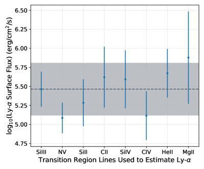
Figure 2: Ly$\alpha$ estimates with 1$\sigma$ uncertainties (blue data points) calculated from each of the measured transition region lines in Table 3 using Equation 1. We take the weighted average as the Ly$\alpha$ flux and 1$\sigma$ uncertainty for K2-3 (grey dashed line and shaded grey area).

2.1.2 Data gap and negative flux

There is a gap in the COS data from 2127–2767Å due to the configuration of the G230L grating. In this case we also do not zero out the flux since it is apparent that there is a non-zero average flux on either side of the data gap, likely representing a small detection of the stellar continuum. We draw a sloped line from the average of the flux on one side of the gap to the average of the flux on the other side. Integrating across this slope will return an average flux value from both sides of the data gap.

We find this an acceptable treatment of the data gap when compared to broadband UV coverage by the XMM-Newton and Swift observatories (further discussed in Section 2.2). The UV photometry from these observations spans parts of the data gap, and the measured fluxes are less than one order of magnitude greater than our estimate for the flux in the gap. The UV photometry should be considered an upper limit, though, since it includes prominent lines on either side of the data gap, including the He ii and Mg ii lines. Any lines in the data gap are relatively weak and would likely not have been visible above the COS noise floor for this target.

At many wavelengths the COS pipeline returns negative flux values, meaning that we are not able to detect any continuum flux from the star. However these negative values can be problematic for photochemical models that do not expect non-physical negative flux. Following the treatment of the MUSCLES spectra v2.2, we “adaptively bin” the data such that negative flux values are balanced by the positive flux in nearby wavelength bins (France et al., 2016; Loyd et al., 2016). This method conserves the overall flux across broad regions of the spectrum.

2.2 X-ray

K2-3 was observed with XMM-Newton for a total 19 ks (Observation ID 0862060401, PI S. Joyce). The X-ray observations with the European Photon Imaging Camera pn CCD (EPIC-pn) resulted in a non-detection, but the star was clearly detected in the simultaneous UV observations with the XMM Optical Monitor. Swift observations of K2-3 in June 2020 also resulted in a non-detection in the X-ray range, as would be expected given the lower sensitivity. From the XMM-Newton X-ray observations we place an upper limit on K2-3’s X-ray flux. We calculate this upper limit by extracting a background subtracted count rate from the source region, using an extraction circle of 30^′′ radius which includes 90% of the EPIC-pn point-spread function. The background count rate is measured from a larger region of 60^′′ to reduce error and is then scaled to match the size of the source region. Although no point source was detected, the count rate in the selected source region can still vary over time due to variations in the background flux. This was checked by plotting the lightcurve from both the source region and background measurement region. The pn exposure is 15.7 ks long and the region lightcurves are binned to 100 s time bins.

It is clear from the background region lightcurve that the second half of the observation was affected by a systematically high background count rate. Because the background region lightcurve is subtracted from the source region lightcurve, the corrected source lightcurve shows high variability during the time when the background region count rate was high. A second issue is that the background subtraction appears to overcompensate, leading to some unphysical negative count rates in the corrected source region lightcurve. Because we do not make a detection of K2-3 in the observations and are instead providing an upper limit on its X-ray emission, this overcompensation by the background subtraction would result in a lower value for the K2-3 X-ray flux upper limit than we can actually determine from the observations. To mitigate this issue, we add 0.013 to the final background subtracted count rate in each bin to ensure that the resulting upper-limit is not unrealistically low. The corrected upper-limit on K2-3’s X-ray flux is thus conservative.

The resulting count rate is then passed to PIMMs to calculate the flux. The model parameters used in PIMMs are:

• Detector/grating/filter: XMM pn, none, medium

• Input energy: Set to default based on the energy range used for the XMM pn extraction

• Model: plasma/APEC

• Galactic neutral hydrogen column density: $5\times 10^{18}$ cm^-2 (total column density); the column density per cm³ is $\sim$0.1 cm^-2 (Redfield & Linsky, 2000).

• Abundance: 1 (Solar)

• kT temperature: 6.1 (log($T$) Mega-Kelvin) / 0.1 (keV)

Since the plasma temperature parameter is unknown, we use a range of values for the Astrophysical Plasma Emission Code (APEC; Smith et al., 2001) temperature (0.1085–0.3058 KeV) appropriate for an inactive M-dwarf to produce a range of flux estimates. The upper end of the APEC temperature range provides the highest upper limit value, and we take this as K2-3’s X-ray flux: $1.68\times 10^{-14}$ erg cm^-2 s^-1 across the range 1.24–62Å, using an upper limit count rate of 0.059 counts per second. When incorporating this value into the panchromatic spectrum we divide it across the wavelength range in order to convert the flux to a flux density in  erg cm^-2 s^-1 Å^-1. Integrating the panchromatic spectrum across the X-ray wavelength range returns the flux upper limit.

2.3 Extreme ultraviolet

There are currently no operating observatories that can observe K2-3 in the extreme ultraviolet (EUV=100–912Å). We instead use a tool borrowed from the stellar astrophysics community (e.g., Sanz-Forcada et al., 2003) that uses flux measured in the UV and X-ray to estimate the EUV. This approach is described in full detail in Duvvuri et al. (2021). Briefly, it involves constructing the functional form of K2-3’s differential emission measure (DEM), which describes the line-of-sight relative abundances of ions in the optically thin chromosphere, transition region, and corona under the assumption of collisional ionization equilibrium.

We calculate the DEM for each ion corresponding to measured transition region lines as well as the X-ray upper limit. To do this we calculate the intensity of each measurement and find the associated emissivity contribution function in the CHIANTI atomic database v10.0 using ChiantiPy (Dere et al., 1997; Del Zanna et al., 2021). The X-ray upper limit corresponds to a broad wavelength range so in this case we combine the emissivity functions of all ions in that range. Following previous works (Louden et al., 2017; Duvvuri et al., 2021) we then fit a 5^th-order Chebyshev polynomial to the measured DEMs, using the open source dynamic nested sampler dynesty (Speagle, 2020) to explore the parameter space. We use the same parameters and bounds as Duvvuri et al. (2021). The best fit of that polynomial becomes the DEM function we use to estimate the unmeasured flux in the EUV. In Figure 3 we show the DEMs of the measured flux with uncertainties propagated from the line fitting described in Section 2.1 at their peak formation temperatures, as well as the best fit polynomial function with 1$\sigma$ uncertainty.

Figure 3: Calculated differential emission measures with 1$\sigma$ uncertainties for observed transition region lines in the UV and broadband X-ray flux (blue bars). The best-fit DEM function is shown as an orange line with the shaded orange 1$\sigma$ region.

When incorporating the EUV flux into the panchromatic spectrum of K2-3 we divide the EUV region into broadband chunks of about 25Å each from 62–912Å, and 22Å each from 912–1132Å, after which point the HST/COS data come in. We make this divide at 912Å because this is where the peak of Ly$\alpha$ continuum emission occurs, and is a natural place to divide the spectrum when integrating the EUV versus the FUV, for example. The different bin sizes are chosen to end in round numbers, which can help avoid small numerical differences when integrating different regions of the spectrum. Similar to what we do for the broadband X-ray data, we take the flux in each bin and divide it by the bin size in order to get the flux density for the panchromatic spectrum.

2.4 Optical and infrared

To fill out the spectrum of K2-3, we append to the high-energy portion a BT-Settl model spanning the optical to mid-infrared (Allard, 2014), which extends to 10$\mu$m. From a grid of BT-Settl models we interpolate to the effective temperature and surface gravity of K2-3.

2.5 Putting it all together

We combine all of the pieces of K2-3’s spectrum and provide four versions of the resulting panchromatic spectrum as high level science products, all available at doi 10.17909/t9-fqky-7k61 (catalog 10.17909/t9-fqky-7k61):

• Variable resolution

• Constant resolution at 1Å

• Variable resolution, adaptively binned to remove negative flux

• Constant resolution at 1Å, adaptively binned to remove negative flux

These data products are designed to match those of the MUSCLES program (France et al., 2016); studies using the MUSCLES spectra should therefore be able to easily incorporate the spectrum of K2-3. We also provide the data from the COS G130M, G160M, and G230L gratings after we have binned the output data from the COS pipeline. The spectrum at constant resolution is shown in Figure 4.

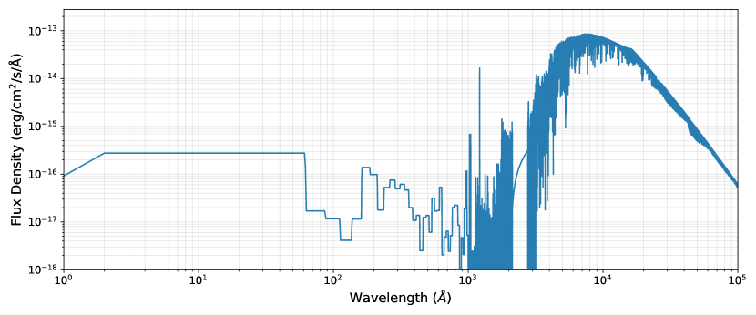
Figure 4: Panchromatic spectrum of K2-3 from 1–10⁵Å and binned to 1Å bins. A high level science product containing this spectrum can be found at doi: 10.17909/t9-fqky-7k61 (catalog 10.17909/t9-fqky-7k61)

.

2.6 Comparison to other M stars

We provide some benchmark properties of K2-3’s high-energy spectrum in Table 4. K2-3 fits with the high-energy trends for M dwarfs established by the MUSCLES survey (France et al., 2016), though no star in the MUSCLES sample is directly analogous to K2-3, an inactive early M star. For instance, K2-3 falls closely in line with the trend in FUV/NUV flux ratio that decreases towards higher effective temperatures. With an effective temperature of $3844^{+61}_{-63}$ K, K2-3 fills in a gap in the MUSCLES sample between early- to mid-M dwarfs and late K dwarfs (see Figure 7 of France et al., 2016). Finally, we calculate the energy-limited hydrodynamic mass loss rate for each of the K2-3 planets as

$$\dot{M}=\frac{3\beta^{2}\eta F_{\mathrm{XUV,p}}}{4KG\rho_{\mathrm{p}}}$$ (2)

where $\eta=\eta_{\mathrm{eva}}$, $\beta$ relates the planet radius to the radius at which XUV flux (= 1–912Å) can be absorbed, $F_{\mathrm{XUV,p}}$ is the XUV flux at the planet, $K$ is a correction factor that accounts for mass only needing to reach the Hill radius to escape, and $\rho_{\mathrm{p}}$ is the planet density (Erkaev et al., 2007; Salz et al., 2016). In this calculation we use the XUV flux each planet currently receives from the host star (Erkaev et al., 2007), and we use prescriptions for the atmospheric expansion $\beta$ and escape efficiency $\eta_{\mathrm{eva}}$ from Salz et al. (2016). We provide these values for each of the K2-3 planet in Table 4. They will come into play later when we discuss the range of atmospheric cases we test for each planet in Section 4.1.

Table 4: Derived Values from the Spectrum of K2-3

	Wavelength (Å)	Value
$\mathrm{log_{10}}(L_{\mathrm{Bol}})$	1–105	$32.35$
$f$(XUV)	1–912	$-4.39$
$f$(FUV)	912–1700	$-4.35$
$f$(NUV)	1700–3200	$-3.33$
FUV/NUV	—	$0.10$
Ly$\alpha$/FUV	—	$0.53\pm 0.42$
		b	c	d
FXUVa	1–912	$5.77\times 10^{2}$	$1.75\times 10^{2}$	$0.79\times 10^{2}$
$\beta$b	—	1.67	1.75	1.76
$\eta_{\mathrm{eva}}$b	—	0.26	0.31	0.32
$\dot{M}$c	—	$16.56\times 10^{8}$	$5.20\times 10^{8}$	$2.36\times 10^{8}$

Note. — Following France et al. (2016), $f\mathrm{(band)}=\mathrm{log}_{10}(L_{\mathrm{band}}/L_{\mathrm{Bol}})$; $F_{\mathrm{Bol}}=9.68\times 10^{-10}$ in all cases.

^a The XUV flux (erg cm^-2 s^-1) at K2-3b, c, d is calculated using median values from a global computed with EXOFASTv2 (Section 3, Table 6).

^b Values for atmospheric expansion $\beta$ and escape efficiency $\eta_{\mathrm{eva}}$ calculated according to Salz et al. (2016).

^c The hydrodynamic mass loss rate (g s^-1), also computed with median values from the global EXOFASTv2 fit. In the case of K2-3d, which does not have a measured mass, we use the 3$\sigma$ observational upper limit of $2.2\mathrm{M}_{\oplus}$. A higher mass for K2-3d would increase its surface gravity and decrease its hydrodynamic mass loss rate, thereby lengthening the timescale for mass loss.

3 K2-3 System Parameters

K2-3 was observed during the K2 mission, which took place after the initial Kepler mission ended due to failure of two out of four reaction wheels (Howell et al., 2014). The K2 phase of the Kepler mission did not point at the same patch of sky that Kepler stared at for four years, but rather moved around the ecliptic in multiple campaigns lasting roughly 80 days each. K2-3 was identified in K2 Campaign 1 (Crossfield et al., 2015). The K2-3 planets have been the subject of numerous follow-up observations (Kosiarek et al., 2019). Because our goal is to model some possible atmospheres around these worlds we wish to measure the parameters of the K2-3 system, and in particular the radii and masses of the planets, to as high a precision as possible given all of the available data. We update the K2-3 system parameters using EXOFASTv2 (Eastman et al., 2019). All of the data that go into this fit, along with the original publications, can be found in Table 5. We process the K2 light curves using keplersplinev2 in order to remove instrument systematics and outliers. We mask out the transits when fitting the variation in the K2 light curve. Spitzer light curves and RV data are provided by Kosiarek et al. (2019).

Much of the data in Table 5 has already been published (Kosiarek et al., 2019), however the EXOFASTv2 fit we present here incorporates two important updates: 1) we simultaneously fit the RV, transit, and stellar SED data in order to achieve our best-fit values, and 2) we include the updated distance from the Gaia Mission (Gaia Collaboration et al., 2016, 2018). Fitting the planetary and stellar parameters simultaneously is important because these values are related to each other. For instance, the planet transits help to constrain their orbital inclinations, which in turn constrain the planetary masses from the radial velocity data. Transit and radial velocity information works together to constrain planet eccentricities. Including the high precision Gaia DR2 parallaxes to constrain the distance to K2-3 affects the stellar luminosity and therefore significantly decreases the uncertainty in the stellar radius, since the luminosity is related to both the stellar distance and radius and is constrained by fitting the star’s SED. Since transiting planet radii are measured in relation to the host star radius, decreasing the uncertainty in the stellar radius decreases the uncertainty in the planet radius. We also do not assume a zero eccentricity for the planetary orbits. Results of the EXOFASTv2 fit can be found in Table 6.

The EXOFASTv2 code is a powerful and highly flexible tool for fitting exoplanet data sets. Based on the data provided and an initial set of priors, EXOFASTv2 returns a set of posterior distributions for stellar and planetary values as well as jitter and offset terms that allow for simultaneous fitting over multiple data sets from multiple instruments. EXOFASTv2 has been widely used and described in other work (Eastman et al., 2019, and references therein), so we just highlight some of the specific settings we use:

• We use the /noclaret flag in the .pro file (this is the main run script). The /noclaret flag turns off the limb-darkening interpolation, which is incomplete for M dwarfs. Without the interpolation we start from an initial guess at the limb-darkening parameters (Claret & Bloemen, 2011; Eastman et al., 2013) and add a wide uniform prior of $\pm 0.15$.

• EXOFASTv2 can use a stellar evolution model to inform the fit to the stellar parameters. In our fit we use the PAdova and TRieste Stellar Evolution Code (PARSEC; Bressan et al., 2012) by setting the /nomist and /parsec flags in the .pro file. We opt for PARSEC over the MESA Isochrones and Stellar Tracks (MIST; Dotter, 2016) because the PARSEC models have been empirically corrected to match the observed radii of low-mass stars like K2-3 Chen et al. (2014).

• In a recent paper, Tayar et al. (2022) point out a persistent underestimation of uncertainties in reported stellar parameters, particularly in the wake of the high-precision parallaxes and photometric measurements from Gaia, which propagate through to computations of the stellar radius, SED, and effective temperature, and eventually trickle down to the planetary parameters we are trying to constrain. In an upcoming paper, we demonstrate how EXOFASTv2 can indeed reach smaller uncertainties when performing a global fit that allows for a quasi-independent constraint on the stellar density from transit data (J. Eastman, in prep). We place reasonable error floors on parameters set by the SED fit: 2.4% on $T_{\mathrm{eff}}$, 2% on $F_{\mathrm{Bol}}$, and 8% on Fe/H by setting teffsed=0.024d0, fehsed=0.080d0, and fbolsed=0.020d0 in the .pro file. We also manually set a conservative limit on the stellar evolution model error of 5% in the massradius_parsec.pro file (percenterror=0.050d0 in line 260 of commit 78cc86e), which results in an acceptable uncertainty on the stellar mass of 5%. This inflation of the various error floors results in uncertainties in the final stellar parameters that agree with systematic error floors recommended by Tayar et al. (2022), while still allowing EXOFASTv2 to use available information to best constrain the free parameters.

• EXOFASTv2 returns a negative value for the median mass of K2-3d, which is not physical. The Chen & Kipping (2017) mass prediction for K2-3d’s radius is $3.00^{+2.15}_{-1.02}$ M_⊕, which would produce a signal of $K\sim 80$ cm s^-1, within the known systematics of the precision radial velocity instruments used in this study. We note however that the Chen & Kipping (2017) radius-mass relation has a number of detection biases. In cases where we wish to use an estimated value for K2-3d’s mass we follow non-parametric approach to compute masses from radii (Ning et al., 2018), applied to an M-dwarf sample Kanodia et al. (2019), which returns an estimate of $1.89^{+3.36}_{-0.91}M_{\oplus}$. This more conservative mass estimate for K2-3d lies even farther below the systematic noise floor of the radial velocity data.

As a check for the results of the EXOFASTv2 fit we calculate the mass of the star K2-3 using the mass-luminosity-metallicity relation for low-mass stars derived by Mann et al. (2019) using nearby binaries. By providing a star’s K-band magnitude, distance, and metallicity, the associated code will provide a stellar mass to 2-3% uncertainty. Providing these values for K2-3 we get a result of $0.551\pm 0.014$ R_⊙ from the Mann et al. (2019) relation, which is in excellent agreement with the stellar mass we find from the EXOFASTv2 fit (Table 6).

Our final results are consistent with those of Kosiarek et al. (2019), with some improvement on precision (Table 6). The increased precision on the stellar radius decreased the fractional uncertainty in the derived planetary radii from 10% to 4%, and increased precision on the stellar mass decreased the fractional uncertainty in the masses of K2-3b and c from 15% to 13% and from 50% to 30%, respectively. This increased precision on the K2-3 planetary radii and masses is important to narrow the range of atmospheric models we test for each planet. The derived planetary parameters in Kosiarek et al. (2019) use stellar parameters from K2-3 that were constrained using medium-resolution ($R\sim 2000$) spectra (Crossfield et al., 2015). We use the Crossfield et al. (2015) values of $T_{\mathrm{eff}}$ and [Fe/H] as priors in our global EXOFASTv2 fit. Despite these priors, we find that K2-3 has a lower effective temperature and a higher metallicity than was found by Crossfield et al. (2015). We use the values we derive for the planetary masses and radii to place the K2-3 planets in the context of other small planets with measured radii and masses (Figure 5).

Table 5: Input data to EXOFASTv2 for the K2-3 system

Observatory/Instrument	Number of Observations
Transits
	b	c	d
K21	8	4	2
Spitzer/IRAC2,3,4,5 4.5$\mu$m	6	5	4
Radial velocities
HARPS6	132
Magellan II/PFS7	31
HARPS-N6,8	197
Keck I/HIRES5	74

Note. — (1) Crossfield et al. (2015); (2) Beichman et al. (2016); (3) Spitzer GO Program 11026 (PI Werner); (4) Spitzer GO Program 12081 (PI Benneke); (5) Kosiarek et al. (2019); (6) Almenara et al. (2015); (7) Dai et al. (2016); (8) Damasso et al. (2018)

Table 6: K2-3 system parameters

Parameter	Units	Values
Priors
$T_{\mathrm{eff}}$	Effective Temperature (K)	$\cal{N}$(3896, 189)
$[$Fe/H$]$	Metallicity (dex)	$\cal{N}$(-0.32, 0.13)
$\varpi$	Parallax (mas)	$\cal{N}$(22.691, 0.063)
$A_{\mathrm{V}}$	V-band extinction (mag)	$\cal{U}$(0.0, 0.09672 )
Stellar parameters
RAa	HH:MM:SS	11:29:20.49
Dec.a	DD:MM:SS	$-$01:27:18.53
$M_{\mathrm{s}}$	Mass (M⊙)	$0.549^{+0.029}_{-0.027}$
$R_{\mathrm{s}}$	Radius (R⊙)	$0.546^{+0.018}_{-0.016}$
$L_{\mathrm{s}}$	Luminosity (L⊙)	$0.0587^{+0.0018}_{-0.0019}$
$F_{\mathrm{Bol}}$	Bolometric Flux ($\times 10^{-10}$ erg cm-2 s-1)	$9.68^{+0.29}_{-0.31}$
$\rho_{\mathrm{s}}$	Density (g cm-3)	$4.78^{+0.37}_{-0.40}$
log10($g_{\mathrm{s}}$)	Surface gravity (cm s2)	$4.704^{+0.023}_{-0.026}$
$T_{\mathrm{eff}}$	Effective Temperature (K)	$3844^{+61}_{-63}$
$[$Fe/H$]$	Metallicity (dex)	$-0.157^{+0.075}_{-0.080}$
Age	Age (Gyr)	$6.9\pm 4.7$
$A_{\mathrm{V}}$	V-band extinction (mag)	$0.042^{+0.036}_{-0.030}$
$\varpi$	Parallax (mas)	$22.689\pm 0.063$
$d$	Distance (pc)	$44.07\pm 0.12$
Planetary parameters
		b	c	d
$P$	Period (days)	$10.0546535^{+0.0000088}_{-0.0000091}$	$24.646729^{+0.000044}_{-0.000042}$	$44.55603^{0.00013}_{-0.00012}$
$R_{\mathrm{p}}$	Radius (R⊕)	$2.078^{+0.076}_{-0.067}$	$1.582^{+0.057}_{-0.051}$	$1.458^{+0.056}_{-0.051}$
$M_{\mathrm{p}}$	Mass (M⊕)b	$5.11^{+0.65}_{-0.64}$	$2.68\pm 0.85$	$-1.1\pm 1.1$
$T_{0}$	Time of conjunction (BJDTDB)	$2457165.32947\pm 0.00025$	$2457329.85688^{+0.00055}_{-0.00056}$	$2457271.78796\pm 0.00076$
$a$	Semi-major axis (AU)	$0.0747^{+0.0013}_{-0.0012}$	$0.1357^{+0.0023}_{-0.0022}$	$0.2014^{+0.0034}_{-0.0033}$
$i$	Inclination (deg)	$89.40^{+0.34}_{-0.22}$	$89.84^{+0.11}_{-0.14}$	$89.82^{+0.12}_{-0.11}$
$e$	Eccentricity	$0.107^{+0.057}_{-0.059}$	$0.048^{+0.073}_{-0.035}$	$0.091^{+0.120}_{-0.064}$
$\omega$	Argument of periastron (deg)	$188^{+32}_{-34}$	$-180^{+100}_{-110}$	$0^{+140}_{-150}$
$K$	RV semi-amplitude (m s-1)	$2.27\pm 0.28$	$0.88\pm 0.28$	$-0.30^{+0.29}_{-0.30}$
$T_{\mathrm{eq}}$	Equilibrium temperature (K)c	$501.3^{+5.1}_{-5.2}$	$371.8^{+3.8}_{-3.9}$	$305.2^{+3.1}_{-3.2}$
$S$	Instellation (S⊕)c	$10.5\pm 1.0$	$3.17\pm 0.30$	$1.44\pm 0.14$
$R_{\mathrm{p}}/R_{\mathrm{s}}$	Planet-to-star radius ratio	$0.03490^{+0.00041}_{-0.00036}$	$0.02658\pm 0.00032$	$0.02449^{+0.00041}_{-0.00040}$
$a/R_{\mathrm{s}}$	Scaled semi-major axis	$29.44^{+0.74}_{-0.84}$	$53.5^{+1.3}_{-1.5}$	$79.4^{+2.0}_{-2.3}$
$b$	Transit impact parameter	$0.31^{+0.13}_{-0.18}$	$0.14^{+0.13}_{-0.10}$	$0.24\pm 0.16$
$\rho_{\mathrm{p}}$	Density (g cm-3)	$3.11^{+0.49}_{-0.46}$	$3.7\pm 1.2$	$-1.9^{+1.9}_{-2.0}$
log10($g_{\mathrm{p}}$)	Surface gravity (cm s-2)	$3.062^{+0.057}_{-0.063}$	$3.02^{+0.12}_{-0.17}$	$2.31^{+0.37}_{-0.57}$
$e\mathrm{cos}\omega$		$-0.094^{+0.061}_{-0.053}$	$-0.010^{+0.041}_{-0.085}$	$0.00^{+0.13}_{-0.12}$
$e\mathrm{sin}\omega$		$-0.012^{+0.041}_{-0.061}$	$0.001\pm 0.029$	$0.003^{+0.039}_{-0.051}$

Note. — Median values and 68% confidence intervals from a global fit using EXOFASTv2, GitHub commit 78cc86e (Eastman et al., 2019); see Section 3 for details.

^aFrom Gaia DR2 (Gaia Collaboration et al., 2016, 2018); J2000, epoch=2015.5.

^bIn the case of K2-3d, EXOFASTv2 returns a mass value of $-1.1\pm 1.1$ $\mathrm{M_{\oplus}}$, since K2-3d is not detected in the RV data. This gives a 3$\sigma$ upper limit on the mass of K2-3d of 2.2 M_⊕. Based on the measured radius for K2-3d, Kanodia et al. (2019) predict a mass of $1.89^{+3.36}_{-0.91}$ M_⊕ when comparing K2-3d to other planets in their M dwarf sample.

^cThe equilibrium temperature of the planet is calculated according to Equation 1 of Hansen & Barman (2007): $T_{\rm eq}=T_{\rm eff}\sqrt{\frac{R_{\mathrm{s}}}{2a}}$, which assumes no albedo and perfect energy redistribution. The quoted statistical error is likely severely underestimated relative to the systematic error inherent in this assumption.

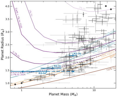
Figure 5: Mass-radius diagram of small planets with measured radii and masses. Black circles are Solar System planets. Radii and masses of the K2-3 planets are from Table 6. K2-3d does not have a measured mass; we plot K2-3d’s measured radius at the position of the 3$\sigma$ upper mass limit ($2.2$ M_⊕). With a dashed line and arrows we also mark the estimate of K2-3d’s mass from a non-parametric fit to a sample of M dwarfs (Kanodia et al., 2019). Composition curves from Zeng et al. (2019). The solid purple composition curves are for an Earth-like core surrounded by an H₂ envelope of various fractional masses at 500 K H₂, which is approximately the equilibrium temperature of K2-3b. We provide one example of a similar composition curve for a 0.1% H₂ atmosphere at 300 K, the approximate equilibrium temperature of K2-3d.

4 Stellar Influence on Planetary atmospheres

4.1 Atmospheric test cases

We combine the high energy information from K2-3 with the revised planetary parameters of K2-3b, c, and d in order to test a range of atmospheric cases for these worlds. We determine the possible H/He envelope mass fraction and maximum water mass fraction for K2-3b and c, using planet interior structure models adapted from Rogers & Seager (2010a, b); Rogers et al. (2011). Because there is no measured mass for K2-3d, we assume a terrestrial composition based on its measured radius. Assuming an Earth-composition core surrounded by a solar composition envelope, the H/He-dominated envelope around K2-3b would comprise $0.36^{+0.14}_{-0.11}\%$ of the planetary mass. For K2-3c this value is $0.07^{+0.09}_{-0.05}\%$. Based on these mass fractions and the energy-limited mass loss rate calculated in Table 4, K2-3b would lose its primordial envelope on a timescale of $2.0^{+0.8}_{-0.6}$ Gyr, while K2-3c would lose its envelope on a timescale of $0.6^{+0.5}_{-0.4}$ Gyr with a 95% upper limit of 1.5 Gyr. Both of these timescales are shorter than the estimated age of the system (Table 6), however see Section 5.1 for more details about potential explanations for the observed K2-3 system architecture.

Both K2-3b and c are also consistent with the end-member case of a 100% H₂O envelope. For the case of a pure water envelope surrounding an Earth-composition core, an H₂O envelope would comprise $55^{+14}_{-12}\%$ of K2-3b’s mass and $16^{+17}_{-10}\%$ of K2-3c’s mass. These water mass fractions could be even higher if mixing between water and an early magma ocean is considered (Dorn & Lichtenberg, 2021). Since we do not have a measured mass for K2-3d therefore do not have any real constraints on its atmosphere, we take this opportunity to showcase the impact of K2-3’s irradiation of K2-3d’s atmospheric composition for several scenarios motivated by Solar System planets: we assume a terrestrial composition for K2-3d and focus on how the high-energy flux from K2-3 would impact Earth- and Venus-like atmospheres around this world.

Based on the compositional constraints of the K2-3 planets, we investigate the following atmospheric scenarios:

• K2-3b: Solar-like envelope; H₂O envelope

• K2-3c: Solar-like envelope; H₂O envelope

• K2-3d: early Venus; modern Venus; modern Earth

4.2 Photochemical modeling of the K2-3 planets

To investigate the impact of the observed stellar spectrum on the atmospheres of each of the planets in the K2-3 system, we use a 1-D photochemical model, Atmos (see Arney et al., 2017, for a full description of the model), in combination with pressure-temperature profiles simulated by HELIOS (Malik et al., 2017). Table 7 lists the major atmospheric constituents for each scenario. Atmos has a long heritage in simulating the atmospheres of rocky planets (e.g., Kasting & Pollack, 1983; Zahnle et al., 2008) which we use in studying the atmosphere of planet d as both a Venus- and Earth-like world. Both modern Venus and modern Earth compositions are taken from observations, while the early Venus scenario is based on simulations by Way & Del Genio (2020) that specify 400 ppm of CO₂ in an N₂-dominated atmosphere. For both early Venus and modern Earth, the tropospheric water abundance is determined from the temperature profile and an assumed relative humidity of $\sim$80%. This underestimates the water vapor feedback but is still broadly consistent with atmospheres that have not yet entered a runaway greenhouse (e.g., Kasting, 1988). Additionally, the higher temperatures reduce ozone abundances in the modern Earth configuration, in line with prior work (Pidhorodetska et al., 2021).

Table 7: Compositions by Atmospheric Type

Type	Composition
Type	Composition
Solar	85.3% H2, 14.6% He, 810 ppm H2O, 400 ppm CH4, 16 ppm CO
Water	99.8% H2O, 0.1% H2, 996 ppm He
Early Venus	98.9% N2, 17.7% H2O, 400 ppm CO2
Modern Venus	96.5% CO2, 2.5% N2, 20 ppm H2O
Modern Earth	21% O2, 15.6% H2O, 360 ppm CO2, 1.8 ppm CH4, 63.4% N2

Atmos has also been modified to handle more diverse planetary scenarios, including warm super-Earths and sub-Neptunes (Harman et al., 2022), which covers the scenarios for planets b and c. These modifications include using higher pressure and temperature thermochemical reactions appropriate for a hydrogen-dominated atmosphere at modest instellation, as well as photolysis of key species, based on the C-H-O chemical scheme from Tsai et al. (2017, 2021). The “surface” is set to the 10-bar pressure level. We assume a vertical eddy diffusion parameter $K_{zz}=10^{9}$ cm² s^-1, noting that different values of $K_{zz}$ (within a few orders of magnitude) have small effects on the atmospheric composition (Harman et al., 2022).

The results of the photochemical simulations are passed to the Planetary Spectrum Generator (PSG; Villanueva et al., 2018) to produce model transmission spectra. With 50 hours of in-transit observing time with JWST/NIRSpec we would achieve a typical uncertainty of 2.7 ppm at a resolution of 25 (Figure 6. The solar composition and H₂O-dominated cases for K2-3b and c are readily differentiated from one another with these simulated observations. For the K2-3d atmospheric cases the 2.7 ppm uncertainty is larger than the total spectral variation (Figure 6; features on the order of 1 ppm). In other words, 50 hours of in-transit observations of K2-3d with JWST/NIRSpec could not distinguish between the three atmospheric cases we explore for this planet. We use the 3$\sigma$ observational upper limit for the mass of K2-3d (2.2 M_⊕) when generating the atmospheric models. We do not include the behavior of aerosols (clouds or hazes) in the model transmission spectra.

To test the influence of the high-energy stellar spectrum on the planetary atmospheres, we run the models again with the input stellar spectrum increased and decreased by a factor of 10. An order of magnitude is about the spread in emission features between similar M dwarfs (France et al., 2016), so with this simple experiment we attempt to address the impact of using a measured high-energy stellar spectrum versus a proxy star. We outline the results for each of the planetary atmospheres:

• For K2-3b there is no change in the volume mixing ratio of prominent molecules like water in either the solar composition or H₂O-dominated cases. This is because at an equilibrium temperature of about 500 K, it is the thermochemistry that dominates the reaction rates in the upper atmosphere.

• For K2-3c, at an equilibrium temperature of about 370 K, the reactions driven by photolysis are on par with those driven by thermochemistry, allowing us to see differences in trace species volume mixing ratios in the solar composition case. In the pure H₂O atmosphere case we do not see any change.

• For K2-3d we test a more complex set of atmospheres and indeed we see a more complicated set of results. Elemental sulfur (S₈), for example, decreases by orders of magnitude as the UV flux increases, implying that for warm to temperate terrestrial planets, a magnitude of uncertainty in the UV will play a significant role in the chemistry of the atmosphere. Molecular oxygen (O₂) also changes, with volume mixing ratio increasing by orders of magnitude in the 10$\times$ more UV flux case compared to the 10$\times$ less UV flux. This demonstrates that under certain UV or T/P conditions on terrestrial worlds, O₂ can arise as an abiotic false positive.

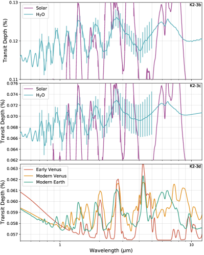
Figure 6: Model transmission spectra for K2-3b, c, and d (top, middle, and bottom panels, respectively) from 0.5 to 12 $\mu$m. Error bars illustrate the typical uncertainty in measuring such atmospheres for K2-3b and c with 50 hr of in-transit observations at a resolution of 25 using JWST/NIRSpec-PRISM. Error bars are not shown for the model atmosphere cases on K2-3d since the uncertainties of 2.7 ppm are much larger than the model atmosphere features. Note the different y-axis scales across the three panels.

5 Discussion

5.1 Explaining the K2-3 system architecture

The K2-3 system is an early-M star orbited by, in increasing orbital distance, a sub-Neptune, a super-Earth enriched in volatiles, and a likely terrestrial super-Earth. It should be noted here that multi-planet systems consisting of small planets are less likely to have a mixture of sub-Neptunes and super-Earths than just one type or the other (Millholland & Winn, 2021). We place the K2-3 planets in the context of the small planet radius valley, extended to a second dimension of planetary instellation (or, similarly, orbital period). When looking at the radius valley for FGK stars (e.g., Figure 10 in Fulton et al., 2017), there is a trend in the location of the radius valley towards increasing planet radius with increasing instellation. When reproducing this figure for stars with $T_{\mathrm{eff}}<4700$ K (spectral type K3.5V and later), the trend in the location of the radius valley appears to flip, and increases in planet radius with decreasing instellation (e.g., Figure 11 of Cloutier & Menou, 2020).

As can be seen in Figure 7, the K2-3 planets appear to fit the bi-modal small planet distribution, with K2-3b falling in the sub-Neptune category and K2-3c and d falling into the super-Earth category, however we should look more closely at these planets together as members of the same multi-planet system to further test theories of planetary formation and evolution. The lines in Figure 7 demonstrate how different planetary formation and evolutionary theories produce trends in the small planet radius valley with planetary instellation that separate the populations of sub-Neptunes from the super-Earths, though the current planet population around low mass stars is not yet large enough to definitively favor one mechanism over the other (Cloutier & Menou, 2020). Focusing on the K2-3 planets together we ask: can planetary formation and evolution models produce the K2-3 system architecture? To answer this question we address each theory below.

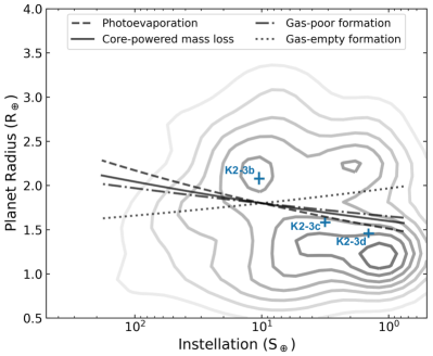
Figure 7: Small planet occurrence rate for planets orbiting cool stars ($T_{\mathrm{eff}}<4700$ K) in radius-instellation space. Occurrence contours are from Cloutier & Menou (2020). Curves represent trends in the radius valley gap as a function of instellation. The trends in $d\ \mathrm{log}\ R_{\mathrm{p}}/d\ \mathrm{log}\ S$ and their sources are as follows: Photoevaporation (0.11; Lopez & Rice, 2018), core-powered mass loss (0.08; Gupta & Schlichting, 2019), gas-poor formation (0.06; Lee & Connors, 2021), gas-empty formation (-0.08; Lopez & Rice, 2018). The K2-3 planets are labeled in blue.

Photoevaporation: We use the publicly available photoevaporation code EvapMass (Owen & Campos Estrada, 2020) to test whether pairs of sub-Neptune and super-Earth planets in the K2-3 system are consistent with photoevaporation, a process by which high-energy stellar flux drives atmospheric mass loss. This process is most effective during the first 100 Myr of a planet’s lifetime when the star is most active. Photoevaporation rates depend on the amount of high-energy XUV stellar flux a planet receives. Because the K2-3 planets orbit the same star, we can take this value out of the equation when comparing the K2-3 planets to each other. We start with the K2-3b and d pair, since K2-3b is a sub-Neptune and K2-3d is potentially a terrestrial world given its radius (Chen & Kipping, 2017; Kanodia et al., 2019). Using stellar and planetary parameters from Table 6, EvapMass calculates the minimum mass of the sub-Neptune K2-3b that would be consistent with photoevaporation if this method were responsible for shaping both K2-3b and K2-3d.

EvapMass cannot find a minimum mass for the sub-Neptune K2-3b assuming that the super-Earth K2-3d has just lost a primordial atmosphere. Put simply, the K2-3d–K2-3b pair are not consistent with photoevaporation. If photoevaporation were solely responsible for the K2-3 system architecture, it would require some combination of K2-3b having a much larger or denser core, or K2-3d orbiting much closer to the star, neither of which is the case. This may not be surprising since the sub-Neptune K2-3b currently receives 7 times more XUV flux than K2-3d (Table 4). EvapMass also does not return a valid result for the K2-3b and c pair, here assuming that K2-3c is the terrestrial world. (This is not a great assumption since K2-3c falls right in the valley between the super-Earth and sub-Neptune distributions, and it’s mass and radius point to volatile enrichment above what is expected for rocky planets.) Owen & Campos Estrada (2020) explored 73 multi-planet Kepler systems with EvapMass and find only two to be inconsistent with photoevaporation. In both cases the system architecture has a sub-Neptune on an orbit between an inner and outer terrestrial planet. In the K2-3 system architecture the sub-Neptune is the inner-most of three planets. It should be noted that there are cases in the Kepler system where a sub-Neptune orbits interior to a super-Earth and the system is still consistent with photoevaporation. We note some assumptions that go into EvapMass in more generally into photoevaporation theory. One is that the planetary cores are all Earth-like surrounded by a $\gtrsim$1% H/He envelope accreted from the protoplanetary disc. As discussed in Section 4.1, the solar composition envelopes for K2-3b and c are disfavored. If instead their atmospheres contain some amount of H₂O they could be more resilient to photoevaporation.

We compare the result from EvapMass to similar calculations aimed at reconciling multi-planet systems with photoevaporation. In Appendix A of Cloutier et al. (2020) the authors lay out a set of inequalities to determine the minimum mass of a gaseous sub-Neptune (or maximum mass of a rocky super-Earth) to satisfy the photoevaporation model. Because inequalities depend on both masses and radii, we test a grid of models that encompasses the range of possible masses and radii for K2-3d (we use the range of masses predicted by Kanodia et al. (2019)). We keep the mass and radius of K2-3b, along with semi-major axes of both planets, fixed to the median values from Table 6. We find that when taking into account the uncertainty in the radius and mass of K2-3d, K2-3b–K2-3d pairings in which K2-3d has a bulk density less than about 3.5 g cm^-3 are consistent with photoevaporation. This would mean that K2-3d would have to have some volatile enrichment above what is expected for terrestrial worlds of with similar radii. However we note that, unlike the EvapMass code, the Cloutier et al. (2020) inequalities do not take into account contraction of the primordial envelope over time as material is lost.

Core-powered mass loss: In principle, core-powered mass loss, by which a light H/He envelope can be driven off by energy originating in the planetary core, might explain the K2-3 system architecture. Since the driving energy is left over from planetary formation, a stochastic process, it is possible that K2-3c and d lost most or all of their H/He envelopes while K2-3b was able to maintain one. However, the mechanism of core-powered mass loss relies on energy from the core reaching the outer isothermal layer of a light atmosphere (an atmosphere weighing less than 5% of the planet’s core mass; Ginzburg et al., 2016), but the rate at which this happens depends on the atmospheric sound speed $c_{s}$, which is itself a function of the planet’s equilibrium temperature (Gupta & Schlichting, 2019). In this way, core-powered mass loss takes into account the distance of the planet from the star. Thus, if we make the assumption that the K2-3 planets were born with identical H/He envelopes, the core-powered mass loss mechanism also disfavors the observed system architecture.

Cloutier et al. (2020) also provide an inequality that must be satisfied for a multi-planet system to be a viable outcome of core-powered mass loss (appendix B of that paper). Based on equations laid out in Ginzburg et al. (2018); Gupta & Schlichting (2019), it is necessary for the cooling timescale of a sub-Neptune planet (like K2-3b) to be greater than the cooling timescale of a super-Earth (like K2-3d) in the same system. As with the photoevaporation case, we test a grid of inequalities corresponding to the range of possible masses and radii for K2-3d. Given the dependence of the cooling timescales on equilibrium temperature, we again find that if K2-3b and d both formed with H/He envelopes, their current architecture cannot be easily explained solely by core-powered mass loss. K2-3b and K2-3d pairings that satisfy the core-powered mass loss inequality would give K2-3d a lower bulk density than expected for a terrestrial world.

Gas-poor formation: Another explanation of the small planet radius valley is that this distribution is baked in at formation. In this picture, the inner region of a protoplanetary disk becomes depleted in gas towards the end of the disk lifetime. At this point protoplanetary cores in the inner disk can cross orbits, collide, and grow. Small amounts of gas escape from the gas-rich outer disk to feed the gas-poor inner disk, which can be acquired by the growing cores (Lee & Chiang, 2016). In this way sub-Neptunes and super-Earths can form in situ. Late-time gas accretion alone can reproduce the small planet radius valley for FGK stars, with super-Earths favored closer to their stars (Lee & Connors, 2021). Post-processing by photoevaporation and/or core-powered mass loss can further turn some of the sub-Neptune population into super-Earths, improving even more the fit to the small planet radius valley for FGK stars. So, while gas-poor formation can reproduce the small planet radius valley, it does not inherently allow for the picture of a sub-Neptune orbiting interior to super-Earths in the same system. It it not certain how this picture would change for planetary formation in M dwarf discs. Recent planetary formation work demonstrates that super-Earth-sized planets can indeed be formed at periods $>$30 d (K2-3b has a period of 44 d), where the influence of photoevaporation and core-powered mass loss is diminished (Lee et al., 2022). However this still does not easily explain the sub-Neptune K2-3b orbiting well interior to K2-3d.

A more extreme formation scenario would be gas-empty formation, in which there is truly no access of late-forming rocky cores to gas from the disc (Lopez & Rice, 2018). Though this can be considered more of a toy model, it does more accurately fit the tentative trend in the small planet radius valley for low-mass stars (Figure 7). However, this model would still have difficulty explaining the K2-3 system architecture because of the model dependency on incident stellar flux, which is a function of the planet orbital distance.

Impact erosion: Finally, we can also consider impact erosion, whereby the collision of material (e.g., asteroids, comets, planetessimals) with a planet surface can cause its atmosphere to either grow or deplete. Whether the impacted planet’s atmosphere grows or depletes is the result of a balance of factors, including the speed, size, impact angle, and volatile content of the impactor, as well as the mass of the impacted planet’s atmosphere and escape velocity. However, when calculating the effects of impact erosion on terrestrial planets, Wyatt et al. (2020) include a dependence on the planet’s orbital location: the erosional efficiency of an impact includes assumptions about the atmospheric scale height, which in turn depends on the planet’s semi-major axis. This results in the conclusion that, all else being equal, terrestrial planets closer to their stars are more likely to lose their atmospheres after an impact than those farther away. Wyatt et al. (2020) do not consider planets with thick H/He envelopes, but the general conclusion does not line up with the observed K2-3 system architecture.

An extreme variation on impact erosion is a late-stage giant impact, whereby the impact can lead to atmospheric loss not only at the site of the impact but also globally due to shocks propagating through the planet (Schlichting et al., 2015). Though close-in planets are again more susceptible to giant impacts because the extent of their isothermal outer envelopes depends on their equilibrium temperatures (Biersteker & Schlichting, 2019), the stochasticity of the giant impact process makes for a tempting, though somewhat fine-tuned, explanation for the K2-3 system: perhaps K2-3c and d started out more like sub-Neptune worlds, only to suffer late-stage giant impacts in which most of their low mean molecular weight envelopes were removed. This might leave K2-3c and d mostly rocky but enhanced with volatile material, as observed.

Finally, we address the fact that the EUV estimate of K2-3 and the resulting mass loss rates depend on our assumptions about the X-ray emission from K2-3, for which we only have an upper limit. As a rough check, we estimate the X-ray flux from K2-3 by translating its rotation period (40 d; Kosiarek et al., 2019) into an X-ray luminosity using the relations from Wright et al. (2018). The result is an estimated X-ray flux of $2.35\times 10^{-15}$ erg cm^-2 s^-1, almost an entire order of magnitude less than our assumed upper limit. Propagating this value through to the estimated EUV flux of K2-3, and further onto the mass loss rates of the planets K2-3b and c, we find that these worlds would lose their H/He envelopes in approximately 5.6 and 1.8 Gyr, respectively. While this would mean that K2-3b may indeed be in the process of losing its primordial atmosphere and will eventually turn into a stripped core, the 1.8 Gyr timescale of hydrodynamic mass loss for K2-3c is at the lowest end of the estimated age of K2-3, making it unlikely that K2-3c is still in the process of losing a primordial atmosphere. We are therefore skeptical that photoevaporation or core powered mass loss can explain the overall architecture of the K2-3 system.

5.2 Prospects for habitable conditions on K2-3d

The outer-most (known) planet of the K2-3 system has a terrestrial-like radius but no measured mass, and sits at the inner edge of K2-3’s habitable zone (Kopparapu et al., 2014). If K2-3d is relatively water-poor, it may have clement surface conditions and liquid water near the poles (e.g., Abe et al., 2011). Alternatively, as a synchronously rotating planet, K2-3d could feature a thick sub-stellar cloud deck that would extend the inner edge of the habitable zone to higher instellation (e.g., Yang et al., 2013; Kopparapu et al., 2017). However, since K2-3d receives roughly 1.4 times Earth’s insolation, it could be in the moist greenhouse regime (Kopparapu et al., 2017), although the threshold for this regime varies based on a number of planetary parameters, including whether or not there is a surface ocean to efficiently distribute heat around the planet (Yang et al., 2019).

K2-3d may be further enriched in volatiles, and in particular water, than the compositions of Zeng et al. (2019) imply (Figure 5). For instance, if K2-3d did manage to accrete H/He from the protoplanetary nebula, surface pressures would be high enough to support a surface magma ocean into which water would readily mix. This would lead to an increase in the estimated water mass fraction given the observed planet radius, compared to the simpler picture of a silicate rock surrounded by a layer of volatiles (Dorn & Lichtenberg, 2021). This presents an intriguing picture for habitability for K2-3d, which could have water locked up in its mantle. Having lost its H/He envelope, or never having had one in the first place, we speculate that this could lead K2-3d to possess a water-rich secondary atmosphere. However, such an atmosphere would likely transition into a runaway greenhouse state due to the high instellation, increasing the apparent volatile abundance over its actual inventory (e.g., Turbet et al., 2019). If, for example, K2-3d has an Earth-like water inventory, the higher XUV fluxes from K2-3 would drive rapid atmospheric escape and evolve the planet towards a modern Venus-like state (Figure 6).

6 Conclusion

In this work we investigate the K2-3 system using a blend of observations and theory. Because the K2-3 planets span the radius-mass space of small exoplanets we can use these worlds as testing grounds for atmospheric and planet evolution models over a range of instellations and compositional cases.

We measure the high-energy spectrum of K2-3 directly using HST/COS in the UV and XMM-Newton in the X-ray. We use this information to estimate regions of K2-3’s high energy spectrum that we cannot measure directly, such as the Ly$\alpha$ line and the EUV, via the differential emission measure method (Duvvuri et al., 2021). We combine the high-energy measurements and estimates with a BT-Settl stellar atmosphere model (Allard, 2014) in order to construct a panchromatic spectrum of K2-3 that can be passed to atmospheric models.

We use all available radial velocity and transit data of the K2-3 planets along with precise parallaxes from Gaia in order to perform a joint fit using the EXOFASTv2 package. The result yields precise radius measurements of the K2-3 planets down to 4% precision. The masses remain more uncertain. The masses of K2-3b and c are constrained to 13% and 30%, respectively, while the outermost world K2-3d is not detected in the radial velocity measurements so we estimate its mass using empirical radius-mass correlations from Chen & Kipping (2017). These radius and mass measurements allow us to constrain the maximum and minimum water/hydrogen envelope mass fractions for K2-3b and c, which both show evidence of volatile-enhanced compositions relative to a terrestrial Earth-like composition (Figure 5).

We model several potential atmospheric compositions for all three of the known planets in the K2-3 system, focusing on solar composition and pure-water atmospheres for the two innermost planets, b and c, and exploring three rocky planet atmosphere scenarios for planet d—early Venus, modern Venus, and modern Earth. K2-3d is located on the cusp of the inner edge of the habitable zone, and could possess an atmosphere that is water-rich or water-poor, depending on how the planet and host star evolved. If K2-3d did accrete an H/He envelope from the protoplanetary nebula before losing it, it may have locked up a substantial amount of water in its mantle during a prolonged magma ocean phase, which could lead to a Venus-like atmosphere today.

Finally, while the K2-3 planets as individual worlds fit nicely into the bi-modal distribution of small planet radii, when scrutinized as a whole system the K2-3 planet properties present challenges to current theories of planet formation and evolution. We find that while K2-3b can maintain a H/He envelope in the presence of host star K2-3, the overall system architecture does not easily fit with the photoevaporation and core-powered mass loss mechanisms to explain the super-Earth–sub-Neptune radius valley. Given that we do not have a measured mass for K2-3d, and because K2-3c has a terrestrial-like radius but is enhanced in volatiles, it is possible that this system is exhibiting the outcomes of the more stochastic processes of planet formation and evolution. We posit that the three K2-3 planets are enhanced in volatiles as an outcome of the planet formation process, subsequent planet migration, post-formation delivery of volatile material, or impact erosion.

We thank Ryan Cloutier, Beatriz Campos Estrada, João Mendonça, Victoria Antoci, René Tronsgaard Rasmussen, Evgenya Shkolnik, Amber Medina, and Zoe Oliver-Grey for helpful discussions during the preparation of this manuscript. This work is based on observations made with the NASA/ESA Hubble Space Telescope, obtained at the Space Telescope Science Institute. Support for program #15110 was provided by NASA through a grant from the Space Telescope Science Institute, which is operated by the Association of Universities for Research in Astronomy, Inc., under NASA contract NAS5-26555. This work has made use of data from the European Space Agency (ESA) mission Gaia (https://www.cosmos.esa.int/gaia), processed by the Gaia Data Processing and Analysis Consortium (DPAC, https://www.cosmos.esa.int/web/gaia/dpac/consortium). Funding for the DPAC has been provided by national institutions, in particular the institutions participating in the Gaia Multilateral Agreement. This work makes use of the CHIANTI atomic database. CHIANTI is a collaborative project involving George Mason University, the University of Michigan (USA), University of Cambridge (UK) and NASA Goddard Space Flight Center (USA). This research has made use of the NASA Exoplanet Archive, which is operated by the California Institute of Technology, under contract with the National Aeronautics and Space Administration under the Exoplanet Exploration Program.

Data products are available as HLSPs at MAST: 10.17909/t9-fqky-7k61 (catalog 10.17909/t9-fqky-7k61).

References

- Abe et al. (2011) Abe, Y., Abe-Ouchi, A., Sleep, N. H., & Zahnle, K. J. 2011, Astrobio., 11, 443, doi: 10.1089/ast.2010.0545
- Allard (2014) Allard, F. 2014, in Exploring the Formation and Evolution of Planetary Systems, ed. M. Booth, B. C. Matthews, & J. R. Graham, Vol. 299, 271–272, doi: 10.1017/S1743921313008545
- Almenara et al. (2015) Almenara, J. M., Astudillo-Defru, N., Bonfils, X., et al. 2015, A&A, 581, L7, doi: 10.1051/0004-6361/201525918
- Arney et al. (2017) Arney, G. N., Meadows, V. S., Domagal-Goldman, S. D., et al. 2017, ApJ, 836, 49, doi: 10.3847/1538-4357/836/1/49
- Beichman et al. (2016) Beichman, C., Livingston, J., Werner, M., et al. 2016, ApJ, 822, 39, doi: 10.3847/0004-637X/822/1/39
- Biersteker & Schlichting (2019) Biersteker, J. B., & Schlichting, H. E. 2019, MNRAS, 485, 4454, doi: 10.1093/mnras/stz738
- Bressan et al. (2012) Bressan, A., Marigo, P., Girardi, L., et al. 2012, MNRAS, 427, 127, doi: 10.1111/j.1365-2966.2012.21948.x
- Chen & Kipping (2017) Chen, J., & Kipping, D. 2017, ApJ, 834, 17, doi: 10.3847/1538-4357/834/1/17
- Chen et al. (2014) Chen, Y., Girardi, L., Bressan, A., et al. 2014, MNRAS, 444, 2525, doi: 10.1093/mnras/stu1605
- Claret & Bloemen (2011) Claret, A., & Bloemen, S. 2011, A&A, 529, A75, doi: 10.1051/0004-6361/201116451
- Cloutier & Menou (2020) Cloutier, R., & Menou, K. 2020, AJ, 159, 211, doi: 10.3847/1538-3881/ab8237
- Cloutier et al. (2020) Cloutier, R., Eastman, J. D., Rodriguez, J. E., et al. 2020, AJ, 160, 3, doi: 10.3847/1538-3881/ab91c2
- Crossfield et al. (2015) Crossfield, I. J. M., Petigura, E., Schlieder, J. E., et al. 2015, ApJ, 804, 10, doi: 10.1088/0004-637X/804/1/10
- Dai et al. (2016) Dai, F., Winn, J. N., Albrecht, S., et al. 2016, ApJ, 823, 115, doi: 10.3847/0004-637X/823/2/115
- Damasso et al. (2018) Damasso, M., Bonomo, A. S., Astudillo-Defru, N., et al. 2018, A&A, 615, A69, doi: 10.1051/0004-6361/201732459
- Del Zanna et al. (2021) Del Zanna, G., Dere, K. P., Young, P. R., & Landi, E. 2021, ApJ, 909, 38, doi: 10.3847/1538-4357/abd8ce
- Dere et al. (1997) Dere, K. P., Landi, E., Mason, H. E., Monsignori Fossi, B. C., & Young, P. R. 1997, A&AS, 125, 149, doi: 10.1051/aas:1997368
- Diamond-Lowe et al. (2021) Diamond-Lowe, H., Youngblood, A., Charbonneau, D., et al. 2021, The Astronomical Journal, 162, 10, doi: 10.3847/1538-3881/abfa1c
- Dorn & Lichtenberg (2021) Dorn, C., & Lichtenberg, T. 2021, ApJ, 922, L4, doi: 10.3847/2041-8213/ac33af
- Dotter (2016) Dotter, A. 2016, ApJS, 222, 8, doi: 10.3847/0067-0049/222/1/8
- Douglas et al. (2014) Douglas, S. T., Agüeros, M. A., Covey, K. R., et al. 2014, ApJ, 795, 161, doi: 10.1088/0004-637X/795/2/161
- Duvvuri et al. (2021) Duvvuri, G. M., Sebastian Pineda, J., Berta-Thompson, Z. K., et al. 2021, ApJ, 913, 40, doi: 10.3847/1538-4357/abeaaf
- Eastman (2017) Eastman, J. 2017, EXOFASTv2: Generalized publication-quality exoplanet modeling code. http://ascl.net/1710.003
- Eastman et al. (2013) Eastman, J., Gaudi, B. S., & Agol, E. 2013, PASP, 125, 83, doi: 10.1086/669497
- Eastman et al. (2019) Eastman, J. D., Rodriguez, J. E., Agol, E., et al. 2019, arXiv e-prints, arXiv:1907.09480. https://arxiv.org/abs/1907.09480
- Erkaev et al. (2007) Erkaev, N. V., Kulikov, Y. N., Lammer, H., et al. 2007, A&A, 472, 329, doi: 10.1051/0004-6361:20066929
- France et al. (2016) France, K., Loyd, R. O. P., Youngblood, A., et al. 2016, ApJ, 820, 89, doi: 10.3847/0004-637X/820/2/89
- Fulton & Petigura (2018) Fulton, B. J., & Petigura, E. A. 2018, AJ, 156, 264, doi: 10.3847/1538-3881/aae828
- Fulton et al. (2017) Fulton, B. J., Petigura, E. A., Howard, A. W., et al. 2017, AJ, 154, 109, doi: 10.3847/1538-3881/aa80eb
- Gaia Collaboration et al. (2016) Gaia Collaboration, Prusti, T., de Bruijne, J. H. J., et al. 2016, A&A, 595, A1, doi: 10.1051/0004-6361/201629272
- Gaia Collaboration et al. (2018) Gaia Collaboration, Brown, A. G. A., Vallenari, A., et al. 2018, A&A, 616, A1, doi: 10.1051/0004-6361/201833051
- Ginzburg et al. (2016) Ginzburg, S., Schlichting, H. E., & Sari, R. 2016, ApJ, 825, 29, doi: 10.3847/0004-637X/825/1/29
- Ginzburg et al. (2018) —. 2018, MNRAS, 476, 759, doi: 10.1093/mnras/sty290
- Green et al. (2012) Green, J. C., Froning, C. S., Osterman, S., et al. 2012, ApJ, 744, 60, doi: 10.1088/0004-637X/744/1/60
- Gupta & Schlichting (2019) Gupta, A., & Schlichting, H. E. 2019, MNRAS, 487, 24, doi: 10.1093/mnras/stz1230
- Hansen & Barman (2007) Hansen, B. M. S., & Barman, T. 2007, ApJ, 671, 861, doi: 10.1086/523038
- Harman et al. (2022) Harman, C. E., Kopparapu, R. K., Stefánsson, G., et al. 2022, \psj, 3, 45, doi: 10.3847/psj/ac38ac
- Howell et al. (2014) Howell, S. B., Sobeck, C., Haas, M., et al. 2014, PASP, 126, 398, doi: 10.1086/676406
- Kanodia et al. (2019) Kanodia, S., Wolfgang, A., Stefansson, G. K., Ning, B., & Mahadevan, S. 2019, ApJ, 882, 38, doi: 10.3847/1538-4357/ab334c
- Kasting (1988) Kasting, J. F. 1988, Icarus, 74, 472, doi: 10.1016/0019-1035(88)90116-9
- Kasting & Pollack (1983) Kasting, J. F., & Pollack, J. B. 1983, Icarus, 53, 479, doi: 10.1016/0019-1035(83)90212-9
- Kopparapu et al. (2014) Kopparapu, R. K., Ramirez, R. M., SchottelKotte, J., et al. 2014, ApJ, 787, L29, doi: 10.1088/2041-8205/787/2/L29
- Kopparapu et al. (2017) Kopparapu, R. K., Wolf, E. T., Arney, G., et al. 2017, ApJ, 845, 5, doi: 10.3847/1538-4357/aa7cf9
- Kosiarek et al. (2019) Kosiarek, M. R., Crossfield, I. J. M., Hardegree-Ullman, K. K., et al. 2019, AJ, 157, 97, doi: 10.3847/1538-3881/aaf79c
- Landi et al. (2012) Landi, E., Del Zanna, G., Young, P. R., Dere, K. P., & Mason, H. E. 2012, ApJ, 744, 99, doi: 10.1088/0004-637X/744/2/99
- Lee & Chiang (2016) Lee, E. J., & Chiang, E. 2016, ApJ, 817, 90, doi: 10.3847/0004-637X/817/2/90
- Lee & Connors (2021) Lee, E. J., & Connors, N. J. 2021, ApJ, 908, 32, doi: 10.3847/1538-4357/abd6c7
- Lee et al. (2022) Lee, E. J., Karalis, A., & Thorngren, D. P. 2022, arXiv e-prints, arXiv:2201.09898. https://arxiv.org/abs/2201.09898
- Lopez & Fortney (2013) Lopez, E. D., & Fortney, J. J. 2013, ApJ, 776, 2, doi: 10.1088/0004-637X/776/1/2
- Lopez & Rice (2018) Lopez, E. D., & Rice, K. 2018, MNRAS, 479, 5303, doi: 10.1093/mnras/sty1707
- Louden et al. (2017) Louden, T., Wheatley, P. J., & Briggs, K. 2017, MNRAS, 464, 2396, doi: 10.1093/mnras/stw2421
- Loyd et al. (2016) Loyd, R. O. P., France, K., Youngblood, A., et al. 2016, ApJ, 824, 102, doi: 10.3847/0004-637X/824/2/102
- Malik et al. (2017) Malik, M., Grosheintz, L., Mendonça, J. M., et al. 2017, AJ, 153, 56, doi: 10.3847/1538-3881/153/2/56
- Mann et al. (2019) Mann, A. W., Dupuy, T., Kraus, A. L., et al. 2019, ApJ, 871, 63, doi: 10.3847/1538-4357/aaf3bc
- Martinez et al. (2019) Martinez, C. F., Cunha, K., Ghezzi, L., & Smith, V. V. 2019, ApJ, 875, 29, doi: 10.3847/1538-4357/ab0d93
- Melbourne et al. (2020) Melbourne, K., Youngblood, A., France, K., et al. 2020, AJ, 160, 269, doi: 10.3847/1538-3881/abbf5c
- Millholland & Winn (2021) Millholland, S. C., & Winn, J. N. 2021, ApJ, 920, L34, doi: 10.3847/2041-8213/ac2c77
- Newton et al. (2017) Newton, E. R., Irwin, J., Charbonneau, D., et al. 2017, ApJ, 834, 85, doi: 10.3847/1538-4357/834/1/85
- Ning et al. (2018) Ning, B., Wolfgang, A., & Ghosh, S. 2018, ApJ, 869, 5, doi: 10.3847/1538-4357/aaeb31
- Owen & Campos Estrada (2020) Owen, J. E., & Campos Estrada, B. 2020, MNRAS, 491, 5287, doi: 10.1093/mnras/stz3435
- Owen et al. (2020) Owen, J. E., Shaikhislamov, I. F., Lammer, H., Fossati, L., & Khodachenko, M. L. 2020, Space Sci. Rev., 216, 129, doi: 10.1007/s11214-020-00756-w
- Owen & Wu (2013) Owen, J. E., & Wu, Y. 2013, ApJ, 775, 105, doi: 10.1088/0004-637X/775/2/105
- Pidhorodetska et al. (2021) Pidhorodetska, D., Moran, S. E., Schwieterman, E. W., et al. 2021, AJ, 162, 169, doi: 10.3847/1538-3881/ac1171
- Redfield & Linsky (2000) Redfield, S., & Linsky, J. L. 2000, ApJ, 534, 825, doi: 10.1086/308769
- Rogers (2015) Rogers, L. A. 2015, ApJ, 801, 41, doi: 10.1088/0004-637X/801/1/41
- Rogers et al. (2011) Rogers, L. A., Bodenheimer, P., Lissauer, J. J., & Seager, S. 2011, ApJ, 738, 59, doi: 10.1088/0004-637X/738/1/59
- Rogers & Seager (2010a) Rogers, L. A., & Seager, S. 2010a, ApJ, 712, 974
- Rogers & Seager (2010b) —. 2010b, ApJ, 716, 1208, doi: 10.1088/0004-637X/716/2/1208
- Salz et al. (2016) Salz, M., Schneider, P. C., Czesla, S., & Schmitt, J. H. M. M. 2016, A&A, 585, L2, doi: 10.1051/0004-6361/201527042
- Sanz-Forcada et al. (2003) Sanz-Forcada, J., Brickhouse, N. S., & Dupree, A. K. 2003, ApJS, 145, 147, doi: 10.1086/345815
- Schlichting et al. (2015) Schlichting, H. E., Sari, R., & Yalinewich, A. 2015, Icarus, 247, 81, doi: 10.1016/j.icarus.2014.09.053
- Smith et al. (2001) Smith, R. K., Brickhouse, N. S., Liedahl, D. A., & Raymond, J. C. 2001, ApJ, 556, L91, doi: 10.1086/322992
- Speagle (2020) Speagle, J. S. 2020, MNRAS, 493, 3132, doi: 10.1093/mnras/staa278
- Tayar et al. (2022) Tayar, J., Claytor, Z. R., Huber, D., & van Saders, J. 2022, ApJ, 927, 31, doi: 10.3847/1538-4357/ac4bbc
- Tsai et al. (2017) Tsai, S.-M., Lyons, J. R., Grosheintz, L., et al. 2017, ApJS, 228, 20, doi: 10.3847/1538-4365/228/2/20
- Tsai et al. (2021) Tsai, S.-M., Malik, M., Kitzmann, D., et al. 2021, ApJ, 923, 264, doi: 10.3847/1538-4357/ac29bc
- Turbet et al. (2019) Turbet, M., Ehrenreich, D., Lovis, C., Bolmont, E., & Fauchez, T. 2019, A&A, 628, A12, doi: 10.1051/0004-6361/201935585
- Van Eylen et al. (2018) Van Eylen, V., Agentoft, C., Lundkvist, M. S., et al. 2018, MNRAS, 479, 4786, doi: 10.1093/mnras/sty1783
- Villanueva et al. (2018) Villanueva, G. L., Smith, M. D., Protopapa, S., Faggi, S., & Mandell, A. M. 2018, Journal of Quantitative Spectroscopy and Radiative Transfer, 217, 86, doi: 10.1016/j.jqsrt.2018.05.023
- Way & Del Genio (2020) Way, M. J., & Del Genio, A. D. 2020, Journal of Geophysical Research: Planets, 125, e2019JE006276, doi: 10.1029/2019JE006276
- Wright et al. (2018) Wright, N. J., Newton, E. R., Williams, P. K. G., Drake, J. J., & Yadav, R. K. 2018, MNRAS, 479, 2351, doi: 10.1093/mnras/sty1670
- Wyatt et al. (2020) Wyatt, M. C., Kral, Q., & Sinclair, C. A. 2020, MNRAS, 491, 782, doi: 10.1093/mnras/stz3052
- Yang et al. (2019) Yang, J., Abbot, D. S., Koll, D. D., Hu, Y., & Showman, A. P. 2019, ApJ, 871, 29, doi: 10.3847/1538-4357/aaf1a8
- Yang et al. (2013) Yang, J., Cowan, N. B., & Abbot, D. S. 2013, ApJ, 771, L45, doi: 10.1088/2041-8205/771/2/L45
- Youngblood et al. (2016) Youngblood, A., France, K., Loyd, R. O. P., et al. 2016, ApJ, 824, 101, doi: 10.3847/0004-637X/824/2/101
- Youngblood et al. (2017) —. 2017, ApJ, 843, 31, doi: 10.3847/1538-4357/aa76dd
- Zahnle et al. (2008) Zahnle, K., Haberle, R. M., Catling, D. C., & Kasting, J. F. 2008, JGR:P, 113, doi: 10.1029/2008JE003160
- Zeng et al. (2019) Zeng, L., Jacobsen, S. B., Sasselov, D. D., et al. 2019, Proceedings of the National Academy of Science, 116, 9723, doi: 10.1073/pnas.1812905116