Extended planetary chaotic zones

Abstract

We consider the chaotic motion of low-mass bodies in two-body high-order mean-motion resonances with planets in model planetary systems, and analytically estimate the Lyapunov and diffusion timescales of the motion in multiplets of interacting subresonances corresponding to the mean-motion resonances. We show that the densely distributed (though not overlapping) high-order mean-motion resonances, when certain conditions on the planetary system parameters are satisfied, may produce extended planetary chaotic zones — “zones of weak chaotization,” — much broader than the well-known planetary connected chaotic zone, the Wisdom gap. This extended planetary chaotic zone covers the orbital range between the 2/1 and 1/1 resonances with the planet. On the other hand, the orbital space inner (closer to the host star) with respect to the 2/1 resonance location is essentially long-term stable. This difference arises because the adiabaticity parameter of subresonance multiplets specifically depends on the particle’s orbit size. The revealed effect may control the structure of planetesimal disks in planetary systems: the orbital zone between the 2/1 and 1/1 resonances with a planet should be normally free from low-mass material (only that occasionally captured in the first-order 3/2 or 4/3 resonances may survive); whereas any low-mass population inner to the 2/1 resonance location should be normally long-lived (if not perturbed by secular resonances, which we do not consider in this study).

Keywords: celestial mechanics: resonances – planetary systems: dynamical evolution and stability: individual: Solar system, HR 8799

1 Introduction

The orbital architectures of planetary systems are established as results of complex cosmogonical and dynamical processes, which include planetary formation, close encounters, scattering, migration in gas-dust disks. On the other hand, selection effects favor discoveries of long-term stable systems. That is why applications of stability criteria are necessary for explaining the observed multitude of architectures of exoplanetary systems.

In this article, we reveal the existence of a weakly unstable multi-resonant zone of dominant perturbative planetary influence, which we call the extended planetary chaotic zone (EPCZ). It covers the orbital range between the 2/1 and 1/1 mean-motion resonances with the planet. Though weak, it is by far more unstable (in a number of senses) than the orbital zone with smaller orbital periods, inner to the 2/1 resonance. We argue that observed structural patterns of planetesimal disks, such as the 2/1 resonance cut-off, may arise due to this effect.

The article is organized as follows. In Section 2, we briefly review relevant theoretical issues on chaotic resonance multiplets (including the standard map theory) in Hamiltonian dynamics, concentrating on how the Lyapunov exponents and diffusion rates in resonance multiplets can be estimated analytically. In Section 3, we apply the theory to characterize the chaotic mean-motion resonances in planetary systems. In Sections 4, 5, and 6, we characterize the resonances massively, building the Farey trees of resonances in model planetary systems. In Section 7, we compute covering factors of dynamical chaos, as a function of test particles’ orbit size, in the same model systems. Section 8 is devoted to general discussions and conclusions.

2 Lyapunov and diffusion timescales in resonance multiplets

We adopt a model of perturbed nonlinear resonance given by the paradigmatic Hamiltonian

$$H={{{\cal G}p^{2}}\over 2}-{\cal F}\cos\phi+a\cos(\phi-\tau)+b\cos(\phi+\tau)$$ (1)

(Shevchenko, 1999, 2000), where the first two terms in equation (1) represent the Hamiltonian $H_{0}$ of the unperturbed pendulum, and periodic perturbations are represented by the last two terms; $\phi$ is the pendulum angle (the resonance phase angle), $p$ is the momentum, $\tau$ is the phase angle of perturbation, $\tau=\Omega t+\tau_{0}$, and $\Omega$ is the perturbation frequency, $\tau_{0}$ is the initial phase of the perturbation; ${\cal F}$, ${\cal G}$, $a$, $b$ are constants.

Many resonant systems in physics and astronomy can be canonically transformed to the perturbed pendulum model, which is thus considered in some sense as a “universal” or “first fundamental” model of nonlinear resonance; see Chirikov (1979); Shevchenko (2020) for details. In a generalized form, the perturbed pendulum model of nonlinear resonance is given by Hamiltonian (1). In the next section, we will see that this model perfectly corresponds to a Hamiltonian description of high-order mean-motion resonances, considered henceforth in this work.

In equation (1), the phase $\phi$ represents a linear resonant combination of the angles of any original system; in the next section, examples of such representation are given. The momentum $p$ is proportional to the time derivative of $\phi$. The momentum $p$ and phase $\phi$ form a pair of conjugated canonical variables of the system defined by the Hamiltonian (1). The system in non-autonomous, as the Hamiltonian explicitly depends on time; thus, the system has one and a half degrees of freedom.

The small-amplitude libration frequency of the system on the resonance modelled by the pendulum is $\omega_{0}=({\cal FG})^{1/2}$. The “adiabaticity parameter”, characterizing the relative frequency of perturbation, is defined as

$$\lambda={\Omega\over\omega_{0}}$$ (2)

(Shevchenko, 2020).

The unperturbed resonance full width is defined as the maximum distance (in momentum $p$) between its separatrices; it is equal to $4({\cal F}/{\cal G})^{1/2}$. Therefore, the adiabaticity parameter $\lambda$ characterizes the distance (in momentum $p$) between the guiding and perturbing resonances in units of one quarter of the full resonance width.

The rate of divergence of close trajectories (in the phase space and in the logarithmic scale of distances) is characterized by the maximum Lyapunov exponent. If the maximum Lyapunov exponent is greater than zero, then the motion is chaotic (Chirikov, 1979; Lichtenberg & Lieberman, 1992). The inverse of this quantity, $T_{\rm L}\equiv L^{-1}$, is the Lyapunov time. It represents the characteristic time of predictable dynamics.

On the other hand, knowledge of diffusion timescales allows one to judge on the possibility for effective transport in action-like variables in the phase space of motion.

The Hamiltonian (1) includes three trigonometric terms, corresponding to three interacting resonances, forming a resonance triplet. Let the number of resonances in a resonance multiplet be greater than three. In the case of non-adiabatic chaos ($\lambda\gtrsim 1/2$) one may still apply, as an approximation, the theory developed in Shevchenko (2014) for the triplet case, because the influence of the “far-away” resonances is exponentially small with $\lambda$. However, if chaos is adiabatic ($\lambda\lesssim 1/2$), the triplet approximation is no more valid for the multiplet comprising more than three resonances. Therefore, let us consider a limit case, namely, the case of infinitely many interacting equal-sized and equally spaced resonances. The standard map

$$y_{i+1} = y_{i}+K\sin x_{i}\ \ \ (\mbox{mod }2\pi),$$

$$x_{i+1} = x_{i}+y_{i+1}\ \ \ (\mbox{mod }2\pi),$$ (3)

describes the motion in just this case, as it is clear from its Hamiltonian:

$$H=\frac{y^{2}}{2}+k\sum_{n=-M}^{M}\cos(x-nt)$$ (4)

(Chirikov, 1979), where $M=\infty$, $k=K/(2\pi)^{2}$. The variables $x_{i}$, $y_{i}$ of the map (3) correspond to the variables $x(t_{i})$, $y(t_{i})$ of the continuous system (4) taken stroboscopically at time moduli $2\pi$ (see, e. g., Chirikov 1979). Alongside with $\lambda$, the standard map stochasticity parameter $K$ can be as well regarded as a measure of resonance overlap, because the adiabaticity parameter for the standard map is $\lambda\equiv\Omega/\omega_{0}=2\pi K^{-1/2}$ (Shevchenko, 2020).

A formula for the maximum Lyapunov exponent of the standard map at $K$ much greater than the critical value $K_{\mathrm{G}}=0.9716...$, i.e., at $K\gg 1$, was derived by Chirikov (1979):

$$L_{\mathrm{st}}\approx\ln\frac{K}{2}.$$ (5)

Already at $K=6$ the difference between the theoretical and numerical-experimental values of $L$ becomes less than $\approx 2\%$ (Chirikov, 1979).

The mapping period $T_{\mathrm{map}}$ of the map (3) can be expressed in original time units of the system (4). Therefore, for the maximum Lyapunov exponent of system (4), at $K\gg 1$ (or, at $\lambda\ll 1$), one has

$$L\approx\frac{L_{\mathrm{st}}}{T_{\mathrm{map}}},$$ (6)

where time is expressed in original time units. For the whole interval of definition of $K$, we use the approximate numerical and theoretical $L(K)$ functions obtained in Shevchenko (2004a, b) for the main chaotic domain of the standard map phase space at any $K$:

$$L(K)=\frac{1}{T_{\mathrm{map}}}\cdot\begin{cases}0.1333K,&\text{if $K<1.1$},\\ 0.469(K-1.037)^{1/2},&\text{if $1.1\leq K<4.4$},\\ \ln\frac{K}{2}+\frac{1}{K^{2}},&\text{if $K\geq 4.4$},\end{cases}$$ (7)

where

$$K=(2\pi/\lambda)^{2},$$ (8)

and $T_{\mathrm{map}}$ is the perturbation period.

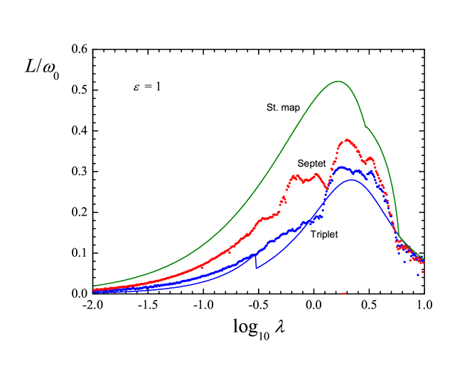
Figure 1: The $\lambda$ dependences of the maximum Lyapunov exponent (normalized by $\omega_{0}$) in resonance multiplets. Dots: numerical-experimental data of Shevchenko (2014). Green (upper) solid curve: the standard map theory (given by equations (7)) for the “infinitet”. Blue (lower) curve: the separatrix map theory for the equally-spaced equally-sized triplet, as described in Shevchenko (2014). Adapted from (Shevchenko, 2014, Fig. 7).

The $\lambda$ dependences, both numerical and theoretical, of the maximum Lyapunov exponent (normalized by $\omega_{0}$) in multiplets of equal-sized and equally spaced resonances are shown in Fig. 1. Note that the normalization by $\omega_{0}$ means that the given normalized maximum Lyapunov exponent is adimensional.

In Fig. 1, the curve for the septet occupies an intermediate position between the curve for the triplet and the curve for the “infinitet”, i. e., for the standard map. Notwithstanding the large perturbation amplitude (resonances are equal in size: in particular, for the triplet given by equation (1) one has $\varepsilon\equiv a/{\cal F}=b/{\cal F}=1$), the numerical data for the triplet agrees well with the separatrix map theory presented in Shevchenko (2014); in Fig. 1, this theory provides the lower solid curve.

The subresonances in the infinitet (the standard map case) start to overlap, on decreasing $\lambda$, at $K_{\mathrm{G}}=0.9716\ldots$ (Chirikov, 1979; Meiss, 1992), i.e., at $\lambda=2\pi K_{\mathrm{G}}^{-1/2}\approx 6.37$. Therefore, the range in $\lambda$ in Fig. 1 almost totally corresponds to the overlap conditions, except at $\log_{10}\lambda\gtrsim 0.8$.

The diffusion coefficient $D$ is defined as the mean-square spread in a selected variable per time unit (Chirikov, 1979; Meiss, 1992); in the standard map model, the selected variable is $y$. If $y$ is not taken moduli $2\pi$, then its variation is unbounded if $K>K_{\mathrm{G}}$. At $K\gg 1$, the Lyapunov time $\approx\ln\frac{K}{2}$ (Equation (5)), and even adjacent iterated values of the phase variables can be regarded as practically independent. Then, the normal diffusion in $y$ at $K\gg 1$ has the rate

$$D=\frac{\langle(\Delta y)^{2}\rangle}{t}=\frac{1}{2}K^{2}$$ (9)

(Chirikov, 1979).

According to Chirikov (1979), in the whole range $1<K<\infty$, the diffusion time, characterizing the mean time of transition between neighbouring integer resonances, $T_{\mathrm{d}}\propto 1/D$, is given by

$$T_{\mathrm{d}}^{\mathrm{map}}\simeq\begin{cases}100\,(K-1)^{-3},&\text{if $1<K\lesssim 4$},\\ 8\pi^{2}K^{-2},&\text{if $K\gtrsim 4$},\end{cases}$$ (10)

which at $K\gg 1$ corresponds to the quasilinear diffusion law (9). Generally, the standard map theory for the diffusion rate is expected to be adequate if the number of resonances in a considered resonance multiplet is large.

3 Chaotic mean-motion resonances

In the vicinities of high-order mean-motion two-body and three-body resonances, the equations of motion are approximately reducible to those of pendulum with periodic perturbations, given by the Hamiltonian (1); see Shevchenko (2020). This reduction provides an opportunity to analytically estimate the Lyapunov and diffusion timescales of the motion, as described in the previous Section.

Let us consider the restricted elliptical planar three-body problem, with a passively gravitating test particle orbiting around a primary mass $m_{1}$ and perturbed by the secondary mass $m_{2}<m_{1}$. In the vicinity of a mean-motion resonance $(k+q)/k$ (where $k\geq 1$ and $q\geq 1$ are integers) with the gravitating binary, the Hamiltonian of the particle’s barycentric motion can be approximately represented as

$$H={1\over 2}\beta\Lambda^{2}-\sum_{p=0}^{q}\varphi_{k+q,k+p,k}\cos(\psi+p\varpi)\approx{1\over 2}\beta\Lambda^{2}-\sum_{p=0}^{q}\varphi_{k+q,k+p,k}\cos(\psi-p\Omega t)$$ (11)

(Holman & Murray, 1996; Murray & Holman, 1997), where $\beta={3k^{2}}/a^{2}$, $\Lambda=\Psi-\Psi_{\mathrm{res}}$, $\Psi=\left[(1-\mu)a\right]^{1/2}/k$, $\Psi_{\mathrm{res}}=\left[(1-\mu)^{2}/(k^{2}(k+q)n_{\mathrm{b}})\right]^{1/3}$, $\mu=m_{2}/(m_{1}+m_{2})$; $\varpi$ is the longitude of the tertiary’s (particle’s) pericentre; $a$ and $e$ are the tertiary’s semimajor axis and eccentricity; $t$ is time, and the frequency $\Omega$ is defined below in equation (15). The angle $\psi\equiv kl-(k+q)l_{\mathrm{b}}$, where $l$ and $l_{\mathrm{b}}$ are the mean longitudes of the tertiary and the primary binary.

The units are chosen in such a way that the total mass ($m_{1}+m_{2}$) of the primary binary, the gravitational constant, the primary binary’s semimajor axis $a_{\mathrm{b}}$ are all equal to one. The binary’s mean longitude $l_{\mathrm{b}}=n_{\mathrm{b}}t$, and its mean motion $n_{\mathrm{b}}=1$, i. e., the time unit equals the ${1\over 2\pi}$th part of the binary’s orbital period. The binary’s period $P_{\mathrm{b}}$ is set to $2\pi$; its mean motion $n_{\mathrm{b}}=1$ and semimajor axis $a_{\mathrm{b}}=1$.

The momentum $\Lambda$ and phase $\psi$ form a pair of conjugated canonical variables of the system defined by the Hamiltonian (11); they can be put in correspondence to the momentum $p$ and phase $\phi$ of the “first fundamental” model Hamiltonian (1). We see that the model (1) can be put in correspondence to the Hamiltonian description (11) of high-order mean-motion resonances, considered henceforth.

The system (11) concerns the case of the outer (with respect to the particle) perturber: the tertiary (the test particle) orbits inside the secondary’s (the perturber’s) orbit around the primary.

Note that the d’Alembert rule concerning the zero sum of integer coefficients in the resonant angles is of course satisfied, but indirectly, because the secondary’s constant longitude of pericentre is set equal to zero (on the d’Alembert rules see Morbidelli 2002).

The integer non-negative numbers $k$ and $q$ define the resonance: the ratio $(k+q)/k$ equals the ratio of the mean motions of the tertiary (the particle) and the secondary (the perturber) in exact resonance.

As described by equation (11), if the perturber’s orbit is eccentric ($e_{\mathrm{b}}>0$), then the resonance $(k+q)/k$ splits into a cluster of $q+1$ subresonances $p=0,1,\ldots,q$, whose resonant arguments are given by the formula

$$\phi=\psi+p\varpi=kl-(q+k)l_{\mathrm{b}}+p\varpi.$$ (12)

The coefficients of the resonant terms, derived in Holman & Murray (1996), are given by

$$|\varphi_{k+q,k+p,k}|\approx{\mu\over{2^{q}q\pi a_{\mathrm{b}}}}{q\choose p}\epsilon^{p}\epsilon_{\mathrm{b}}^{q-p},$$ (13)

where $\epsilon={{ea_{\mathrm{b}}}/{|a-a_{\mathrm{b}}|}}$, $\epsilon_{\mathrm{b}}={{e_{\mathrm{b}}a_{\mathrm{b}}}/{|a-a_{\mathrm{b}}|}}$, and ${i\choose j}$ is the binomial coefficient. The approximation (13) is applicable, if $\epsilon q<1$ (Holman & Murray, 1996). Besides, model (11) is restricted to the resonances with $q\geq 2$.

The signs of the coefficients $\varphi_{k+q,k+p,k}$ alternate when $p$ is incremented. Therefore, the coefficients with indices $p$ and $p+2$ always have the same sign. This means that at any choice of the guiding resonance, its closest neighbours in the multiplet have coefficients with equal signs.

In the model (11), the coefficients $\varphi_{k+q,k+p,k}$ are treated as constants. According to Holman & Murray (1996) and Murray & Holman (1997), the frequencies $\omega_{0}$ of small-amplitude librations on subresonances are given by

$$\omega_{0}=(\beta|\varphi_{k+q,k+p,k}|)^{1/2}\approx\frac{n_{\mathrm{b}}}{1-\alpha}\left[(1-\mu)\mu{{2^{2-q}q}\over{3\pi}}{q\choose p}\alpha\epsilon^{p}\epsilon_{\mathrm{b}}^{q-p}\right]^{1/2},$$ (14)

and the perturbation frequency is

$$\Omega\equiv-\dot{\varpi}\approx\frac{\alpha b^{(1)}_{3/2}(\alpha)}{8\left[(1-\mu)a_{\mathrm{b}}\right]^{1/2}}\approx\frac{(1-\mu)\mu}{2\pi}n_{\mathrm{b}}\frac{\alpha^{1/2}}{(1-\alpha)^{2}},$$ (15)

where $b^{(1)}_{3/2}(\alpha)$ is a Laplace coefficient, and

$$\alpha\equiv a/a_{\mathrm{b}}=\left[k/(k+q)\right]^{2/3}.$$ (16)

Following Murray & Holman (1997), for the effective stochasticity parameter $K$ in the subresonance multiplet we take

$$K_{\mathrm{eff}}=\beta\psi_{\mathrm{mid,0}}\left(\frac{\pi}{\mu A}\right)^{2},$$ (17)

where

$$\beta=\frac{3k^{2}}{{a_{\mathrm{b}}}^{2}}\simeq\frac{4q^{2}}{3\epsilon^{2}},$$ (18)

and

$$A=\frac{\alpha b^{(1)}_{3/2}(\alpha)}{8((1-\mu)a_{\mathrm{b}})^{1/2}}\simeq\frac{1}{4\pi}\frac{\alpha^{1/2}}{\epsilon^{2}}.$$ (19)

Further on, for evaluating $\beta$ and $A$, we use the non-approximated expressions, i.e., the first ones in equations (18) and (19). The stochasticity parameter $K$ of the standard map theory (Chirikov, 1979) is the same, in its dynamical sense, as the given $K_{\mathrm{eff}}$; otherwise, in the standard map case, the resonance multiplet is infinite.

For the guiding subresonance we take the strongest one, that in the middle of the multiplet. As soon as $p=0,1,2,3,...,q$, the “middle” value of $p$ is $p_{\mathrm{mid}}=(q+1)/2-1$; and, if $q=1$, then we take $p_{\mathrm{mid}}=1$.

Let us calculate the width of the chaotic multiplet (that with overlapping subresonances, $K>K_{\mathrm{G}}$). First of all, we define technical quantities. For the first subresonance ($p=0$), such quantity is

$$\psi_{0}=\frac{\mu}{\pi q}{q\choose 0}\left(\frac{\epsilon_{\mathrm{b}}}{2}\right)^{q}=\frac{\mu}{\pi q}\left(\frac{\epsilon_{\mathrm{b}}}{2}\right)^{q},$$ (20)

whereas, for the last one ($p=q$),

$$\psi_{q}=\frac{\mu}{\pi q}{q\choose q}\left(\frac{\epsilon_{0}}{2}\right)^{q}=\frac{\mu}{\pi q}\left(\frac{\epsilon_{0}}{2}\right)^{q},$$ (21)

and, for the middle one,

$$\psi_{\mathrm{mid,0}}=\frac{\mu}{2^{q}\pi q}{q\choose p_{0}}\epsilon_{0}^{p_{0}}\epsilon_{\mathrm{b}}^{q-p_{0}}$$ (22)

at $\epsilon=\epsilon_{0}$, and

$$\psi_{\mathrm{mid,max}}=\frac{\mu}{2^{q}\pi q}{q\choose p_{0}}\epsilon_{\mathrm{max}}^{p_{0}}\epsilon_{\mathrm{b}}^{q-p_{0}}$$ (23)

at $\epsilon=\epsilon_{\mathrm{max}}$.

The distance, in the canonical momentum variable, between the subresonances is

$$\delta\Lambda=2\mu A/\beta;$$ (24)

see (Murray & Holman, 1997, equation (28)). For the first and last subresonances in the multiplet, the half-widths are given by

$$\Delta\Lambda_{0}=2(\psi_{0}/\beta)^{1/2},\quad\Delta\Lambda_{q}=2(\psi_{q}/\beta)^{1/2},$$ (25)

and, summing, for the total width $\Delta a_{\mathrm{ch}}$ of the subresonance multiplet one has

$$\Delta a_{\mathrm{ch}}=\frac{2ka_{\mathrm{b}}^{1/2}}{(1-\mu)^{1/2}}\left(q\delta\Lambda+\Delta\Lambda_{0}+\Delta\Lambda_{q}\right).$$ (26)

If $\Delta a_{\mathrm{ch}}<2\Delta\Lambda_{0}$, we take $\Delta a_{\mathrm{ch}}=2\Delta a_{0}$, and if $\Delta a_{\mathrm{ch}}<2\Delta\Lambda_{q}$, we take $\Delta a_{\mathrm{ch}}=2\Delta a_{q}$.

Note that the total width of the chaotic multiplet is calculated here taking into account the half-widths of the boundary subresonances, as bounded by their unperturbed separatrices. The widths of the perturbed (splitted) separatrices can also be calculated (see Shevchenko 2008, 2020), but we ignore them in view of the dominating widths of the considered multiplets themselves.

To apply in the next sections, let us write down also an expression for the half-width $\Delta a_{\mathrm{cr}}$ of the Wisdom gap (the planetary connected chaotic zone). In units of the perturber’s semimajor axis $a_{\mathrm{b}}$, it is given by

$$\Delta a_{\mathrm{cr}}/a_{\mathrm{b}}\approx 1.6\mu^{2/7}$$ (27)

(Duncan, Quinn, & Tremaine, 1989; Murray & Dermott, 1999); concerning the accuracy of the numerical coefficient, see discussion in Shevchenko (2020).

Consider now the diffusion rates. As follows from equation (9), the diffusion coefficients are given by

$$D(I_{0})=\frac{\pi p_{0}^{2}\psi_{\mathrm{mid,0}}^{2}}{2\mu A},$$ (28)

$$D(I_{\mathrm{max}})=\frac{\pi p_{0}^{2}\psi_{\mathrm{mid,max}}^{2}}{2\mu A},$$ (29)

where $I_{0}=e_{0}^{2}/2$, $I_{\mathrm{max}}=e_{\mathrm{max}}^{2}/2$. To compute the removal time, we set $e_{\mathrm{max}}=0.4$, as this eccentricity value is normally sufficient for reaching typical secular resonances in the inner Solar system (see, e.g., Morbidelli 2002).

We do not take the particle’s initial eccentricity equal to a particular constant value (as was adopted in Holman & Murray 1996; Murray & Holman 1997), but take it equal to the forced eccentricity. In the perturber’s vicinity, according to (Hénon & Petit, 1986, equation (33)), the latter is given by

$$e_{\mathrm{f,HP}}=\frac{2.24\,\mu}{(1-\alpha)^{2}},$$ (30)

and, far from the perturber, according to (Heppenheimer, 1978, equation (4)), it is given by

$$e_{\mathrm{f,H}}=\frac{2}{\pi}\cdot\frac{2.5\,\alpha e_{\mathrm{b}}}{(1-{e_{\mathrm{b}}}^{2})}=\frac{5}{\pi}\cdot\frac{\alpha e_{\mathrm{b}}}{(1-{e_{\mathrm{b}}}^{2})}.$$ (31)

This is the time-averaged quantity, hence the coefficient $2/\pi$. At a given value of $a$, if $e_{\mathrm{f,HP}}>e_{\mathrm{f,H}}$, then we take $e_{0}=e_{\mathrm{f,HP}}$, else we take $e_{0}=e_{\mathrm{f,H}}$.

In accord with equations (28) and (29), the diffusion time is therefore given by

$$T_{\mathrm{d}}=\begin{cases}\displaystyle{\frac{p_{I_{0}}p_{I_{\mathrm{max}}}}{\left[D(I_{0})D(I_{\mathrm{max}})\right]^{1/2}},}&\text{if $q>2$},\\ \qquad\displaystyle{\frac{I_{\mathrm{max}}^{2}}{D(I_{0})},}&\text{if $q\leq 2$}.\end{cases}$$ (32)

To use the standard map theory, we set $K=K_{\mathrm{eff}}$.

In the standard map theory, the Lyapunov exponent $L$ is given by formula (7). Therefore, the Lyapunov time for Hamiltonian (11), in the perturber’s orbital periods, can be written down as

$$T_{\mathrm{L}}=\frac{1}{2\mu AL}.$$ (33)

The diffusion time $T_{\mathrm{d}}$ is given by formula (32); therefore, in the perturber’s orbital periods, the removal time is

$$T_{\mathrm{r}}=\frac{1}{2\pi}T_{\mathrm{d}}.$$ (34)

4 The Farey tree of mean-motion resonances

The Farey tree technique is used in the number theory to organize rational numbers (Hardy & Wright, 1979). Here we use it to organize mean-motion resonances in a clear and straightforward way.

The Farey tree is built as follows. Consider some rational numbers $m^{\prime}/n^{\prime}$ and $m^{\prime\prime}/n^{\prime\prime}$ that are “neighbouring”, i.e., $m^{\prime}n^{\prime\prime}-m^{\prime\prime}n^{\prime}=1$. Let them form the first level of the tree. Then, the second level of the tree is formed by a “mediant,” given by the formula $m^{\prime\prime\prime}/n^{\prime\prime\prime}=(m^{\prime}+m^{\prime\prime})/(n^{\prime}+n^{\prime\prime})$. Each next level is formed by taking mediants of the numbers obtained at all preceding levels. Thus, the third level comprises two mediants ($(m^{\prime}+m^{\prime\prime\prime})/(n^{\prime}+n^{\prime\prime\prime})$ and $(m^{\prime\prime\prime}+m^{\prime\prime})/(n^{\prime\prime\prime}+n^{\prime\prime})$) of three numbers at two lower levels, the fourth level comprises four mediants of five numbers at three lower levels, and so on. If, at the first level, one takes $m^{\prime}/n^{\prime}=0$ and $m^{\prime\prime}/n^{\prime\prime}=1$, then the Farey tree, generated up to infinity, will comprise all rational numbers in the [0, 1] closed interval. For details, see (Meiss, 1992, pp. 814–815); a graphical scheme of the Farey tree construction is given in fig. 26 in Meiss (1992).

Concerning the motion inner to the perturber in our planetary problem, the ratio of orbital frequencies (mean motions) of the particle and the perturber is greater than one; therefore, representing mean-motion resonances by rational numbers, we define the resonances as reciprocals of the rational numbers in the Farey tree generated in the [0, 1] segment.

Recall that the order of a mean-motion resonance is given by the difference between the numerator and the denominator in its rational-number representation. It is important that, at each consequent level of the Farey tree, the order of any generated mean-motion resonance may only rise or stay constant; indeed, for the rational-number mediant $m^{\prime\prime\prime}/n^{\prime\prime\prime}=(m^{\prime}+m^{\prime\prime})/(n^{\prime}+n^{\prime\prime})$ the order of the corresponding resonance is $q^{\prime\prime\prime}=n^{\prime}+n^{\prime\prime}-m^{\prime}-m^{\prime\prime}$, i.e., it is equal to $q^{\prime}+q^{\prime\prime}$, the sum of the orders of two lower-level generating resonances. As soon as the orders are non-negative, the generated resonance order cannot decrease. It is also important to note that the Farey tree covers and organizes the full set of rational numbers (Hardy & Wright, 1979; Meiss, 1992); accordingly, it covers and organizes the entire set of mean-motion resonances.

For two generating integer resonances $p/1$ and $(p+1)/1$, the mediant will be $(2p+1)/2$. Therefore, the half-integer resonances are the mediants for the integer ones, and so on. The number of all resonances up to level $k$ is $N_{\mathrm{res}}=2^{k-1}+1$.

For the first and second generating rational numbers at the first level of the Farey tree, we take, respectively, 0/1 and 1/1. They correspond to the mean-motion resonances 1/0 and 1/1 of the particle with the perturber (in its turn, these two resonances correspond to the test particle’s semimajor axis $a=0$ and $a=1$, in units of the perturber’s semimajor axis). Then, following the outlined above algorithm, we obtain the resonances 2/1 (at the second level of the tree); 3/1 and 3/2 (at the third level); 4/1, 5/2, 5/3, 4/3 (at the fourth level); and so on.

5 The “Sun – Jupiter – minor body” model system

Let us consider our Solar system with Jupiter regarded as a unique perturber, i.e., we ignore all other planets. Therefore, in the formulas of Section 3, we set the mass parameter $\mu=1/1047$, the secondary’s eccentricity $e_{\mathrm{b}}=0.048$ and its orbital period $P_{\mathrm{b}}=11.86$ yr.

Using the algorithm described in Section 4, we generate mean-motion resonances in the inner Solar system up to level 10 of the Farey tree, and compute the Lyapunov times, removal times, and widths of the chaotic resonance multiplets, using formulas given in Section 3.

In Fig. 2, we illustrate the mean-motion resonances in the inner Solar system. In the left panel of this Figure, the stochasticity parameter $K$ (blue dots) of the resonances is shown as a function of the tertiary’s semimajor axis $a$. The vertical green line marks the location of the 2/1 resonance with Jupiter. The horizontal magenta and blue dotted lines correspond to $K=K_{\mathrm{G}}$ and $K=4$, respectively. One may see that in the orbital range between the 2/1 and 1/1 resonances the values of $K$ are orders of magnitude greater than those in the range between the 0/1 and 2/1 resonances. In the right panel, the same set of resonances is displayed, but for the product $q\epsilon$ (blue dots). The horizontal red line marks the $q\epsilon=1$ limit. We see that for the most of the high-order resonances, the product $q\epsilon>1$; this means that the adopted theory can be used solely as an extrapolation.

At smaller values of $\mu$ and $e_{\mathrm{b}}$, one may use the theory without any extrapolation, as we demonstrate in the next Section.

In Fig. 3, left panel, the Lyapunov time $T_{\mathrm{L}}$ (olive dots) is shown as a function of the tertiary’s semimajor axis $a$. The vertical green line marks the location of the 2/1 resonance with Jupiter. The vertical red line marks the inner border of the Wisdom gap (the planetary connected chaotic zone) of Jupiter, and the double vertical black, light magenta, blue, and magenta lines mark the borders of the Wisdom gaps of Mercury, Venus, Earth, and Mars, respectively. The Wisdom gap borders’ locations are given by equation (27).

In the right panel, the removal times $T_{\mathrm{r}}$ (olive dots) are shown for the resonances with $K>K_{\mathrm{G}}$. The two panels certify that, in the orbital range between the 2/1 and 1/1 resonances, the $T_{\mathrm{L}}$ and $T_{\mathrm{r}}$ values are orders of magnitude less than those in the range between the 0/1 and 2/1 resonances.

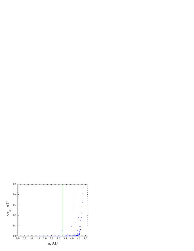
Figure 4: The widths of subresonance multiplets of resonances, in the same model as in Figs 2 and 3. Blue dots: the widths $\Delta a_{\mathrm{ch}}$ of subresonance multiplets. For the resonances with $K<K_{\mathrm{G}}$ the widths are set to zero. Green vertical line: the 2/1 resonance with Jupiter. Red vertical line: the inner border of the Wisdom gap of Jupiter.

In Fig. 4, the widths $\Delta a_{\mathrm{ch}}$ (in tertiary’s semimajor axis) of the subresonance multiplets of mean-motion resonances are displayed (the blue dots). For the resonances with $K<K_{\mathrm{G}}$, the widths are set to zero. The vertical green line marks the location of the 2/1 resonance with Jupiter. The vertical red line marks the inner border of the Wisdom gap of Jupiter. We see that the total width of the chaotic resonances to the left of the 2/1 resonance is just zero, in contrast to the situation to the right of the 2/1 resonance, where a lot of chaotic resonances of significant measure are present.

6 The “star – super-Earth – minor body” model system

Now let us consider a system with a much smaller value of the mass parameter $\mu$: a “Solar-like star – super-Earth” system. Mass of the model super-Earth is set equal to three Earth masses, i.e., $\mu=10^{-5}$; and the super-Earth’s orbit eccentricity $e_{\mathrm{b}}=0.005$. As in the previous Section, we generate the mean-motion resonances in the inner model system up to level 10 of the Farey tree, and calculate the Lyapunov and removal times and the widths of the chaotic subresonance multiplets of the mean-motion resonances.

In Fig. 5, we illustrate the mean-motion resonances in our model exoplanet system. In the left panel of this Figure, the stochasticity parameter $K$ of the chaotic subresonance multiplets of the mean-motion resonances is shown as a function of the tertiary’s semimajor axis $a$ (blue dots). The semimajor axis of the super-Earth orbit is set to one. The vertical green line marks the location of the 2/1 resonance with the super-Earth. The horizontal magenta and blue dotted lines correspond to $K=K_{\mathrm{G}}$ and $K=4$, respectively. As in Section 5 above, one may see that in the range between the 2/1 and 1/1 resonances the values of $K$ are typically orders of magnitude greater than in the range between the 0/1 and 2/1 resonances. Also we display (in the right panel) the same resonances, but for the product $q\epsilon$ (blue dots). The horizontal red line marks the $q\epsilon=1$ limit. We see that for all resonances, the product $q\epsilon<1$; this means that the adopted theory is everywhere valid.

In Fig. 6, left panel, the Lyapunov time $T_{\mathrm{L}}$ (olive dots) is shown is shown as a function of the tertiary’s semimajor axis $a$. The vertical green line marks the location of the 2/1 resonance with the super-Earth. The vertical red line marks the inner border of the super-Earth’s Wisdom gap. In the right panel, the removal times $T_{\mathrm{r}}$ (olive dots) are shown for the resonances with $K>K_{\mathrm{G}}$. As in Section 5 above, the panels of Fig. 6 make it clear that, in the range between the 2/1 and 1/1 resonances, the $T_{\mathrm{L}}$ and $T_{\mathrm{r}}$ values are orders of magnitude smaller than those in the range between the 0/1 and 2/1 resonances.

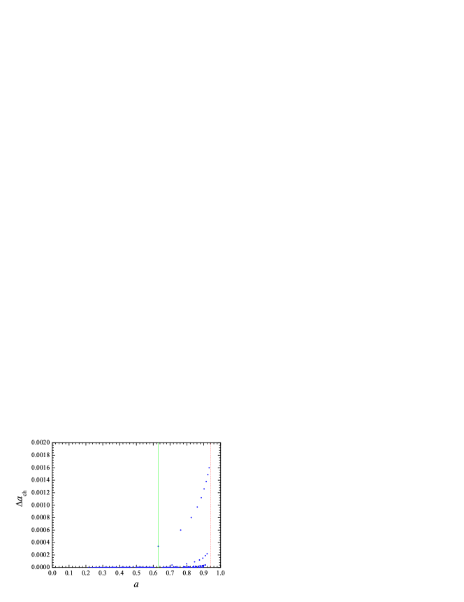
Figure 7: The widths of subresonance multiplets of resonances, in the same model as in Figs 5 and 6. Blue dots: the widths $\Delta a_{\mathrm{ch}}$ of subresonance multiplets. For the resonances with $K<K_{\mathrm{G}}$ the widths are set to zero. Green vertical line: the 2/1 resonance with the super-Earth. Red vertical line: the inner border of the super-Earth’s Wisdom gap.

In Fig. 7, the widths $\Delta a_{\mathrm{ch}}$ (blue dots) of the subresonance multiplets of mean-motion resonances are displayed. For the subresonance multiplets with $K<K_{\mathrm{G}}$, the widths are set to zero. The vertical green line marks the location of the 2/1 resonance with the super-Earth. The vertical red line marks the inner border of the super-Earth’s Wisdom gap. As in Section 5, we see that the total width of chaotic resonances to the left of the 2/1 line is zero, whereas to the right of the 2/1 line there is a lot of broad chaotic resonances.

7 Covering factors of dynamical chaos

Let us define the covering factor of chaos as the sum of the widths of the mean-motion resonances with $K>K_{\mathrm{G}}$ in a particular range of the initial orbital radii of the test minor body. This notion may seem similar to “optical depths,” used in Quillen (2011) and Hadden & Lithwick (2018) to characterize resonance ensembles, but there exists a qualitative difference: the covering factor, as introduced here, concerns chaotic resonances (those with overlapping subresonances), whereas the “optical depths” take into account the widths of all resonances.

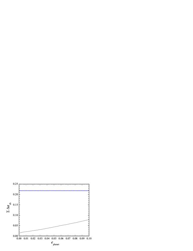
Figure 8: The chaos covering factor in the inner Solar system (the sum of the widths of the mean-motion resonances with $K>K_{\mathrm{G}}$, up to the Farey tree level 10, as a function of Jupiter’s eccentricity $e_{\mathrm{planet}}$ (black solid curve). The widths are in units of Jupiter’s orbital radius. Blue dotted horizontal line: the covering factor (the radial half-width) of the Wisdom gap of Jupiter.

In the model Solar system, defined in Section 5, the sole perturber is Jupiter and, therefore, the mass parameter $\mu=10^{-3}$. The covering factor of chaos in the inner Solar system (apart from the Wisdom gap of Jupiter), for the resonance ensemble up to the Farey tree level 10, is shown, as a function of Jupiter’s eccentricity $e_{\mathrm{planet}}=e_{\mathrm{b}}$, in Fig. 8. The horizontal blue dotted line represents the covering factor (the radial half-width) of the Wisdom gap of Jupiter. We see that the covering factor of the chaotic resonances inner (in orbital radius) to the Wisdom gap is always much less than the covering factor (the relative radial size) of the Wisdom gap itself.

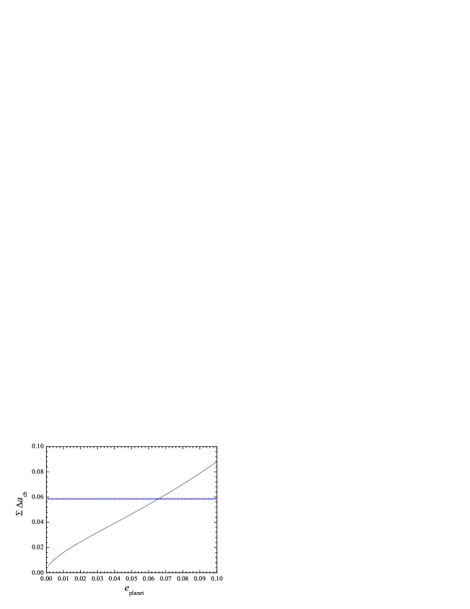
Figure 9: The chaos covering factor in the inner model “Sun-like star – super-Earth – minor body” system (the sum of the widths of the mean-motion resonances with $K>K_{\mathrm{G}}$, up to the Farey tree level 10), as a function of the super-Earth’s eccentricity $e_{\mathrm{planet}}$ (black solid curve). The widths are in units of the super-Earth’s orbital radius. Blue dotted horizontal line: the covering factor (the radial half-width) of the super-Earth’s Wisdom gap.

In the model exoplanet system, as defined in Section 6, the mass parameter $\mu=10^{-5}$. The covering factor of the mean-motion resonances with $K>K_{\mathrm{G}}$ in the inner system up to the Farey tree level 10 is shown, as a function of the planet’s eccentricity $e_{\mathrm{planet}}$, in Fig. 9. The horizontal blue dotted line represents the covering factor (the radial half-width) of the super-Earth’s Wisdom gap. We see that, with increasing the perturber’s eccentricity, the covering factor of the chaotic resonances inner (in orbital radius) to the perturber’s Wisdom gap starts to dominate over the covering factor of the Wisdom gap rather rapidly.

8 Discussion and conclusions

As shown above in Sections 5 and 6, the densely distributed (though not overlapping) high-order resonances, when certain conditions for the planetary system parameters are satisfied, may produce an extended planetary chaotic zone (EPCZ) — the weak instability zone, disconnectedly but densely extending, in orbital radius, the planetary chaotic zone down to the 2/1 resonance with the planet. Therefore, the extended planetary chaotic zone covers the orbital range between the 2/1 and 1/1 resonances with the planet. On the other hand, the orbital space inner to the 2/1 resonance can be essentially long-term stable.

What is the cause of this difference? Let us demonstrate that it can be qualitatively explained as due to a specific behavior of the dependence of the adiabaticity parameter of subresonance multiplets on the value of the particle orbit’s semimajor axis. The adiabaticity parameter is given by equation (2): $\lambda=\Omega/\omega_{0}$. Using equations (14) and (15) for the frequencies $\omega_{0}$ and $\Omega$, one arrives at

$$\lambda={\Omega\over\omega_{0}}=C\cdot(1-\alpha)^{\frac{q}{2}-1},$$ (35)

where $\alpha=a/a_{\mathrm{b}}$, as defined above, and the coefficient $C=C(\mu,q,e,e_{\mathrm{b}})$ does not depend on $\alpha$. One may see that, at $q>2$, $\lambda$ tends to zero, if $\alpha\to 1$, and it tends to $C$, if $\alpha\to 0$.

Equation (35) is valid if the particle’s proper eccentricity is large enough, namely, if it is much greater than the forced eccentricity: $e_{\mathrm{proper}}\gg e_{\mathrm{forced}}$. As mentioned above, the forced eccentricity in immediate vicinities of the perturber is given, according to Hénon & Petit (1986), by equation (30), and, far from the perturber it is given, according to Heppenheimer (1978), by equation (31).

If $e_{\mathrm{proper}}\ll e_{\mathrm{forced}}$, one should substitute $e=e_{\mathrm{forced}}$ in the expression for $\omega_{0}$, equation (14). Then, for the adiabaticity parameter, at locations close to the perturber, one has

$$\lambda=C^{\prime}\cdot(1-\alpha)^{q-1}$$ (36)

with the coefficient $C^{\prime}=C^{\prime}(\mu,q,e_{\mathrm{b}})$. At locations far from the perturber, one has

$$\lambda=C^{\prime\prime}\cdot(1-\alpha)^{\frac{q}{2}-1}\cdot\alpha^{-\frac{q}{4}}$$ (37)

with $C^{\prime\prime}=C^{\prime\prime}(\mu,q,e_{\mathrm{b}})$. Equations (36) and (37) demonstrate that in the whole range $0<\alpha<1$, at $q>1$, the adiabaticity parameter $\lambda$ increases if $\alpha$ is decreased. In other words, $\lambda$ becomes larger for orbits more distant from the perturber and more closer to the host star.

Thus, for high-order mean-motion resonances, either at $e_{\mathrm{proper}}\gg e_{\mathrm{forced}}$ or at $e_{\mathrm{proper}}\ll e_{\mathrm{forced}}$, the adiabaticity parameter $\lambda$ increases if $\alpha$ is decreased from 1 down to 0.

Recall that the chaotic layers, if $\lambda$ is increased, exponentially shrink in width (Chirikov, 1979; Shevchenko, 2008). On the other hand, as it is clear from Figs 2–3 and 5–6, the Farey tree of mean-motion resonances forms two distinct major “nests”, distinctly separated from each other by the 2/1 resonance location at $\alpha=\alpha_{1/2}=2^{-2/3}=0.630...$. The increase of $\lambda$ with decreasing $\alpha$ radically (exponentially with $\alpha\to 0$) suppresses chaos in the nest on the left of $\alpha_{1/2}$ (in the panels of Figs 2–7), in contrast to that on the right of $\alpha_{1/2}$, because the nests are far from each other. In this way, the interplay of the rise of $\lambda$ with decreasing $\alpha$ and the resonance nests’ broad separation explains the rather sharp EPCZ appearance.

The EPCZ phenomenon can be more or less active in determining the architectures of planetary systems: the orbital zone between the 2/1 and 1/1 resonances with a planet can be expected to be normally free from low-mass material and, perhaps, also from less massive (than the perturber) planets. Only the material occasionally captured in the first-order 3/2 or 4/3 resonance may survive, as in the Kepler-223 system.

On the other hand, no restrictions apply to populate the zone inner (in orbital radius) to the 2/1 resonance. In this respect, the sharp difference in the global stability between the 0/1–2/1 and 2/1–1/1 orbital zones seems to agree with available data on the known architectures of planetary systems.

This first of all concerns the observed structure of planetesimal disks, such as the 2/1 resonance cut-off, in observed planetary systems, including our Solar one. The main asteroid belt in the Solar system is cut-off from above at its radial exterior by the 2/1 mean-motion resonance with Jupiter; therefore, if any material have been ever substantially present in the 2/1–1/1 orbital zone (corresponding to the radial space between the 2/1 and 1/1 mean-motion resonances with Jupiter), it has been exhausted, whatever the reason for this removal could have been. Only some small amount of material captured in the first-order 3/2 and 4/3 resonances could have survived. Note that the formation of individual matter-free gaps at the 2/1 resonance is directly observed in numerical experiments, already on relatively short timescales (Demidova & Shevchenko, 2016).

Among observed exoplanet systems, a prominent example of the 2/1-resonance inner cut-off of a circumstellar disk is exhibited in the HR 8799 system. This system is remarkable, being a “young” structural analogue of the Solar system. Indeed, its architecture is similar to that of ours: the orbits of its observed four giant planets are surrounded by a warm dust belt analogous to the asteroid belt in our system, and from outside they are surrounded by a cold belt analogous to the Kuiper belt (Faramaz et al., 2021). The inner part of the system (bounded in radius from above by the “asteroid belt”) contains a zone of potential habitability. According to Faramaz et al. (2021), “simply put, the system of HR 8799 is a younger, broader, and more massive version of the Solar System”. Its “asteroid belt,” in its turn, is cut-off from above by the 2/1 resonance with the giant planet that is innermost in this system, similar to the situation in the Solar system.

What could be the mechanism responsible for any rapid-enough removal of material from the weakly unstable zone? In our Solar system, the Yarkovsky effect and the impact destruction (giving birth to asteroid families) of bodies in the main asteroid belt continuously supply material into numerous chaotic resonant bands present inside the belt. This process monotonously, though slowly, exhausts the belt: in the chaotic bands, the eccentricity is slowly pumped up until the particles enter secular resonances, and the latter drive the material away, mostly up to falling onto the Sun (see, e.g., Morbidelli 2002). Note that the Yarkovsky drift in the semimajor axis, $\mathrm{d}a/\mathrm{d}t$, can be estimated using equations (4)–(5) in Bottke et al. (2006). As illustrated in Fig. 2 in Bottke et al. (2006), it may provide, depending on a number of physical parameters, the rapid-enough permanent radial transport of asteroidal material.

The same removal process is by all means active, to a more or less degree, in planetesimal disks of any exoplanet system. Therefore, it may more or less (depending on the system parameters) rapidly exhaust the EPCZ. For this to occur, the “clearing” (those providing the rapid-enough eccentricity pumping) chaotic resonant bands should have a sufficient covering factor (as defined in Section 7) in orbital radius.

In this article, we have considered the EPCZ formed interior to the planet’s orbit. Any global stability properties of the outer resonance zones require a separate analysis, as they broadly extend to infinity; it would be accomplished elsewhere. In particular, this analysis could shed light on possible resonant/chaotic structure of circumstellar external planetesimal disks, similar to the Solar system’s Kuiper belt, whose resonant structure is mostly controlled by Neptune.

As follows from comparing the numerical results presented in Sections 5 and 6, the dynamical importance of the EPCZ in presence of smaller-$\mu$ perturbers tends to be much greater than in presence of larger-$\mu$ perturbers: indeed, the results indicate that, for the Earths and super-Earths orbiting the Solar-like stars, the removal of material from their EPCZs is expected to be much more pronounced than for the giant planets of similar host stars.

Acknowledgments. The author is most thankful to the referee for comments and remarks. This work was supported in part by the Russian Science Foundation, project 22-22-00046.

Data availability. The data underlying this article will be shared on reasonable request to the corresponding author.

Figure 2: The mean-motion resonances in the inner Solar system up to the Farey tree level 10. Left panel: the stochasticity parameter $K$ (blue dots) as a function of the tertiary’s semimajor axis $a$. Vertical green line: the 2/1 resonance with Jupiter. Magenta and blue dotted horizontal lines: the $K=K_{\mathrm{G}}$ and $K=4$ limits, respectively. Right panel: the product $q\epsilon$ (blue dots) as a function of $a$; red horizontal line: the $q\epsilon=1$ limit.

Figure 3: The Lyapunov and removal times, in the same model as in Fig. 2. Left panel: the Lyapunov time $T_{\mathrm{L}}$ (olive dots) as a function of the tertiary’s semimajor axis $a$. Vertical green line: the 2/1 resonance with Jupiter. Red vertical line: the inner border of the Wisdom gap of Jupiter. Double vertical black, light magenta, blue, and magenta lines: the borders of the Wisdom gaps of Mercury, Venus, Earth, and Mars, respectively. Right panel: the removal time $T_{\mathrm{r}}$ (olive dots) as a function of semimajor axis $a$. Solely the resonances with $K>K_{\mathrm{G}}$ are presented.

Figure 5: The mean-motion resonances in the model “Sun-like star – super-Earth – minor body” system up to the Farey tree level 10. Left panel: the stochasticity parameter $K$ (blue dots) as a function of the tertiary’s semimajor axis $a$. The semimajor axis of the super-Earth is set to one. Green vertical line: the 2/1 resonance with the super-Earth. Magenta and blue dotted horizontal lines: the $K=K_{\mathrm{G}}$ and $K=4$ limits, respectively. Right panel: the product $q\epsilon$ (blue dots) as a function of $a$; red horizontal line: the $q\epsilon=1$ limit.

Figure 6: The Lyapunov and removal times, in the same model as in Fig. 5. Left panel: the Lyapunov time $T_{\mathrm{L}}$ (olive dots) as a function of the tertiary’s semimajor axis $a$. Vertical green line: the location of the 2/1 resonance with the super-Earth. Vertical red line: the inner border of the super-Earth’s Wisdom gap. Right panel: the removal time $T_{\mathrm{r}}$ (olive dots) as a function of semimajor axis $a$. Solely the resonances with $K>K_{\mathrm{G}}$ are presented.

References

- Bottke et al. (2006) Bottke Jr. W.F., et al., 2006, Annu. Rev. Earth Planet. Sci., 34, 157
- Chirikov (1959) Chirikov B.V., 1959, Atomnaya Energiya, 6, 630 (in Russian) [1960, J. Nucl. Energy Part C: Plasma Phys., 1, 253]
- Chirikov (1979) Chirikov B.V., 1979, Phys. Rep., 52, 263
- Demidova & Shevchenko (2016) Demidova T.V., Shevchenko I.I., 2016, MNRAS, 463, L22