Law of large numbers and central limit theorem for wide two-layer neural networks: the mini-batch and noisy case

Abstract

In this work, we consider a wide two-layer neural network and study the behavior of its empirical weights under a dynamics set by a stochastic gradient descent along the quadratic loss with mini-batches and noise. Our goal is to prove a trajectorial law of large number as well as a central limit theorem for their evolution. When the noise is scaling as $1/N^{\beta}$ and $1/2<\beta\leq\infty$, we rigorously derive and generalize the LLN obtained for example in [CRBVE20, MMM19, SS20b]. When $3/4<\beta\leq\infty$, we also generalize the CLT (see also [SS20a]) and further exhibit the effect of mini-batching on the asymptotic variance which leads the fluctuations. The case $\beta=3/4$ is trickier and we give an example showing the divergence with time of the variance thus establishing the instability of the predictions of the neural network in this case. It is illustrated by simple numerical examples.

Keywords. Machine learning, neural networks, law of large numbers, central limit theorem, empirical measures, particle systems, mean field.
AMS classification (2020). 68T07, 60F05, 60F15, 35Q70.

Setting and main results

Introduction

Setting and purpose of this work. Thanks to their impressive results, deep learning techniques have nowadays become standard supervised learning methods in various fields of engineering or research [GBC16]. A robust understanding of their behavior and efficiency is however still lacking and a large effort is put towards achieving mathematical foundations of empirical observations. Among this effort, the case of wide two-layer single network, and its connection with mean-field network, has particularly been fruitful, as considered for example in [RVE18, MMN18, SS20b, SS20a]. In such setting, a convergence towards a limit PDE system can be established when the neuron numbers goes to infinity. The behavior in long time of this limit PDE may then give an easier framework to establish the convergence towards minimizers of the loss function of the neural network. Partial results can be found in this direction [MMN18, CB18] but as underlined in [E20], a lot still remains to be understood and proved mathematically rigorously. In this context, our work is two-fold. First, we will concern ourselves with the mathematical justification of the law of large numbers and central limit theorems of the trajectory of the empirical measure of the weights, under the optimization by a stochastic gradient descent (SGD), with mini-batching and in the presence of noise with a range of scalings. Mini-batch SGD [BCN18] is widely used in machine learning since it allows for shorter training times thanks to parallelisation, while reducing the variance in SGD estimates. How to choose the optimal mini-batch size, and furthermore with theoretical guarantees, remains an active research line [KMN⁺17, SL18, GLQ⁺19]. Introducing noise in SGD, as considered in [MMN18], can lead to better generalisation perfomance thanks to an improved ability to escape saddle points, as shown in [JNG⁺21]. Note that this differs from the analysis approach consisting in directly modelizing the noise of SGD as for instance done in [WHX⁺20, SGN⁺19]. Second we will do so by providing a rigorous framework which could be generalized to study overparametrized limit of other neural networks (e.g. deep ensemble, bayesian neural networks, …). Thus, the benefit of the overparametrized limit and its convexification of the loss landscape through a non-linear PDE could lead in these different architectures to derivations of theoretical guarantees of convergence, while it remains hard to analyse these landscapes directly in the case of a finite number of neurons, even large.

Let us now precise the framework for this paper. Let $(\Omega,\mathcal{F},\mathbf{P})$ be a probability space, and $\mathcal{X}$ and $\mathcal{Y}$ be subsets of $\mathbf{R}^{n}$ ($n\geq 1$) and $\mathbf{R}$ respectively. In this work, we consider the following two-layer neural network

$$g_{W}^{N}(x):=\frac{1}{N}\sum_{i=1}^{N}\sigma_{*}(W^{i},x),$$ (1.1)

where $x\in\mathcal{X}$ denotes the input data, $g_{W}^{N}(x)\in\mathbf{R}$ the output returned by the neural network, $\sigma_{*}:\mathbf{R}^{d}\times\mathcal{X}\rightarrow\mathbf{R}$ the activation function, $N\geq 1$ the number of neurons on the hidden layer, and $W=(W^{1},\dots,W^{N})\in(\mathbf{R}^{d})^{N}$ are the weights to optimize ($d\geq 1$). In the supervised learning setting, a data point $(x,y)\in\mathcal{X}\times\mathcal{Y}$ is distributed according to $\pi\in\mathcal{P}(\mathcal{X}\times\mathcal{Y})$, where $\mathcal{P}(\mathcal{X}\times\mathcal{Y})$ denotes the set of probability measures on $\mathcal{X}\times\mathcal{Y}$. Ideally, one chooses the weights $W=(W^{1},\dots,W^{N})$ as a global minimizer of the risk $\textbf{E}_{\pi}[\mathsf{L}(g_{W}^{N}(x),y)]$, where $\mathsf{L}:\mathbf{R}\times\mathbf{R}\rightarrow\mathbf{R}$ is the so-called loss function ($\textbf{E}_{\pi}$ stands for the expectation when $(x,y)\sim\pi$). In this work, we consider the square loss function out of simplicity, but other loss function or classification problem could be considered, namely:

$$\mathsf{L}(g_{W}^{N}(x),y)=\frac{1}{2}\big{|}g_{W}^{N}(x)-y\big{|}^{2}.$$

Since the risk can not be computed (because $\pi$ is unknown), the parameters are usually learned by stochastic gradient descent. In this work, we consider the mini-batch setting with weak noise, which is defined as follows. First, for $k\geq 0$, consider $((x_{k}^{n},y_{k}^{n}))_{n\geq 1}$ a sequence of random elements on $\mathcal{X}\times\mathcal{Y}$ (each $(x_{k}^{n},y_{k}^{n})$ being distributed according to $\pi$), and $N_{k}$ a random element with values in $\mathbf{N}^{*}=\{1,2,3,\ldots\}$. Then, the mini-batch $B_{k}$ is defined by:

$$B_{k}=\{(x^{1}_{k},y_{k}^{1}),\ldots,(x^{N_{k}}_{k},y^{N_{k}}_{k})\},\text{ in particular $|B_{k}|=N_{k}$, where $|B_{k}|$ denotes the cardinality of $B_{k}$}.$$

In addition, at each iteration of SGD, we add a Gaussian noise term, whose variance is scaled according to $N^{-2\beta}$, with $\beta>\frac{1}{2}$, hence qualified weak. Note that the case of Gaussian noise with $\beta=1/2$ is addressed in [MMN18] and could also be considered here in our setting, but with additional assumptions to integrate the noise in the limit process.

Thus, the SGD algorithm we consider is the following : for $k\geq 0$ and $i\in\{1,\dots,N\}$,

$$\begin{cases}W_{k+1}^{i}=W_{k}^{i}+\displaystyle\frac{\alpha}{N|B_{k}|}\sum_{(x,y)\in B_{k}}(y-g_{W_{k}}^{N}(x))\nabla_{W}\sigma_{*}(W_{k}^{i},x)+\frac{\varepsilon_{k}^{i}}{N^{\beta}},\\ W_{0}^{i}\sim\mu_{0},\end{cases}$$ (1.2)

where $\varepsilon_{k}^{i}\sim\mathcal{N}(0,I_{d})$ and $\mu_{0}\in\mathcal{P}(\mathbf{R}^{d})$. The evolution of the weights is tracked through their empirical distribution $\nu_{k}^{N}$ (for $k\geq 0$) and its scaled version $\mu_{t}^{N}$ (for $t\in\mathbf{R}_{+}$), which are defined as follows:

$$\nu_{k}^{N}:=\frac{1}{N}\sum_{i=1}^{N}\delta_{W_{k}^{i}}\ \text{ and }\ \mu_{t}^{N}:=\nu_{\lfloor Nt\rfloor}^{N}.$$

For an element $\mu\in\mathcal{M}_{b}(\mathbf{R}^{d})$ (the space of bounded countably additive measures on $\mathbf{R}^{d}$), we use the notation

$$\langle f,\mu\rangle_{\mathrm{m}}=\int_{\mathbf{R}^{d}}f(w)\mu(\mathrm{d}w),$$

for any $f:\mathbf{R}^{d}\to\mathbf{R}$ such that $\int_{\mathbf{R}^{d}}f(w)\mu(\mathrm{d}w)$ exists. If no confusion is possible, we simply denote $\langle f,\mu\rangle_{\mathrm{m}}$ by $\langle f,\mu\rangle$. For instance, considering the neural network (1.1), we have, for any $x\in\mathcal{X}$,

$$g_{W_{k}}^{N}(x)=\frac{1}{N}\sum_{i=1}^{N}\sigma_{*}(W^{i}_{k},x)=\langle\sigma_{*}(\cdot,x),\nu_{k}^{N}\rangle,\ \ k\geq 0.$$

In this work, we prove that the the whole trajectory of the scaled empirical measures of the weights defined by (1.2) (namely $\{t\mapsto\mu_{t}^{N},t\in\mathbf{R}_{+}\}_{N\geq 1}$) satisfies a law of large numbers and a central limit theorem, see respectively Theorem 1 and Theorem 2. We also exhibit a particular fluctuation behavior depending on the value of the parameter $\beta$ ruling the weakness of the added noise.

Related works. Law of large numbers and central limits theorems have been obtained for several kinds of mean-field interacting particle systems in the mathematical literature, see for instance [Szn91, HM86, FM97, JM98, DLR19, DMG99, KX04] and references therein. When considering particle systems arising from the SGD-minimization problem in a two-layer neural network, we refer to [MMN18] for a law of large numbers on the empirical measure at fixed times, see also [MMM19]. We also refer to [RVE18] where conditions for global convergence of the GD on the ideal loss and of the SGD with mini-batches increasing in size with $N$, as well as the scaling of the error with the size of the network, are established from formal asymptotic arguments. Doing so, they also observe with increasing mini-batch size in the SGD the reduction of the variance of the process leading the fluctuations of the empirical measure of the weights (see [RVE18, Arxiv-V2. Sec 3.3]), until the mini-batches are large enough to recover the situation of the idealized gradient descent (similar to an infinite batch), which leads to other order of fluctuations (see [RVE18, Arxiv-V2. Prop 2.3]). We also refer to [CRBVE20] for a similar line of work on the GD on the empirical loss. A law of large numbers and a central limit theorem on the whole trajectory of the empirical measure are also obtained in [SS20b, SS20a] for a standard SGD scheme. We also mention the work done in [DBDFS20] on propagation of chaos for SGD with different step-size schemes. In this work, and compared to the existing literature dealing with the SGD minimization problem in two-layer neural networks, we provide a rigorous proof with precise justifications of all steps of the existence of the limit PDE (in particular, uniqueness and relative compactness) in the law of large numbers as well as the limit process for the central limit theorem on the trajectory of the empirical measure. This will be the basis for future works on deep ensembles or overparameterized bayesian neural networks. We furthermore do so in a more general variant of SGD with mini-batching of any size and weak noise (see (1.2)). A noisy SGD was also considered in [MMN18], corresponding to $\beta=1/2$ in our setting, for which they obtain for the LLN a different limit PDE than in the non-noisy case (presence of an additionnal regularizing Laplacian term in the limit equation). While we could recover in a straightforward manner a trajectorial version of [MMN18], we consider here out of concision the range $\beta>1/2$, showing a single limit PDE for the LLN, and obtain a similar result for $\beta>3/4$ for the CLT, while showing analytically for $\beta=3/4$ and numerically for $\beta\leq 3/4$ a particular fluctuation behavior. Furthermore, we analytically show the expected reduction, with the mini-batch size, of the variance of the process leading the fluctuations of the weight empirical measure and numerically display the reduction of the global variance.

Main results

The sequence $\{t\mapsto\mu_{t}^{N},t\in\mathbf{R}_{+}\}_{N\geq 1}$ is studied as a sequence of processes with values in the dual of some (weighted) Hilbert space on $\mathbf{R}^{d}$. These Hilbert spaces are introduced in the next section.

Notation and assumptions

Weighted Sobolev spaces. Following [AF03, Chapter 3], we consider, for a function $g\in\mathcal{C}_{c}^{\infty}(\mathbf{R}^{d})$ (the space of functions $g:\mathbf{R}^{d}\rightarrow\mathbf{R}$ of class $\mathcal{C}^{\infty}$ with compact support), the following norm, defined for $J\in\textbf{N}$ and $b\geq 0$ :

$$\|g\|_{\mathcal{H}^{J,b}}:=\Big{(}\sum_{|k|\leq J}\int_{\mathbf{R}^{d}}\frac{|D^{k}g(x)|^{2}}{1+|x|^{2b}}\mathrm{d}x\Big{)}^{1/2}.$$

Let $\mathcal{H}^{J,b}(\mathbf{R}^{d})$ be the closure of the set $\mathcal{C}_{c}^{\infty}(\mathbf{R}^{d})$ for this norm. The space $\mathcal{H}^{J,b}(\mathbf{R}^{d})$ is a Hilbert space when endowed with the norm $\|\cdot\|_{\mathcal{H}^{J,b}}$. The associated scalar product on $\mathcal{H}^{J,b}(\mathbf{R}^{d})$ will be denoted by $\langle\cdot,\cdot\rangle_{\mathcal{H}^{J,b}}$. We denote by $\mathcal{H}^{-J,b}(\mathbf{R}^{d})$ its dual space. For an element $\Phi\in\mathcal{H}^{-J,b}(\mathbf{R}^{d})$, we use the notation

$$\langle f,\Phi\rangle_{J,b}=\Phi[f],\ f\in\mathcal{H}^{J,b}(\mathbf{R}^{d}).$$

For ease of notation, and if no confusion is possible, we simply denote $\langle f,\Phi\rangle_{J,b}$ by $\langle f,\Phi\rangle$. Let us now define $\mathcal{C}^{J,b}(\mathbf{R}^{d})$ as the space of functions $g:\mathbf{R}^{d}\rightarrow\mathbf{R}$ with continuous partial derivatives up to order $J\in\textbf{N}$ such that

$$\text{for all}\ |k|\leq J,\ \lim_{|x|\rightarrow\infty}\frac{|D^{k}g(x)|}{1+|x|^{b}}=0.$$

This space is endowed with the norm

$$\|g\|_{\mathcal{C}^{J,b}}:=\sum_{|k|\leq J}\ \sup_{x\in\mathbf{R}^{d}}\frac{|D^{k}g(x)|}{1+|x|^{b}}.$$

We also introduce $\mathcal{C}_{b}(\mathbf{R}^{d})$, the space of bounded continuous functions $g:\mathbf{R}^{d}\rightarrow\mathbf{R}$, endowed with the supremum norm. We also denote by $\mathcal{C}^{\infty}_{b}(\mathbf{R}^{d})$ the space of smooth functions over $\mathbf{R}^{d}$ whose derivatives of all order are bounded. We have $\mathcal{C}^{\infty}_{b}(\mathbf{R}^{d})\subset\mathcal{H}^{J,b}(\mathbf{R}^{d})$ as soon as $b>d/2$ (more generally $x\in\mathbf{R}^{d}\mapsto(1-\chi(x))|x|^{a}\in\mathcal{H}^{J,b}(\mathbf{R}^{d})$ if $b-a>d/2$, where $\chi\in\mathcal{C}_{c}^{\infty}(\mathbf{R}^{d},[0,1])$ equals $1$ near $0$).

Weighted Sobolev embeddings. We recall that from [FM97, Section 2],

$$\mathcal{H}^{\ell+j,a}(\mathbf{R}^{d})\hookrightarrow_{\text{H.S.}}\mathcal{H}^{j,a+b}(\mathbf{R}^{d}) \ell>d/2 b>d/2 a,j\geq 0$$ when , , and (1.3)

where $\hookrightarrow_{\text{H.S.}}$ means that the embedding is of Hilbert-Schmidt type, and

$$\text{$\mathcal{H}^{\ell+j,a}(\mathbf{R}^{d})\hookrightarrow\mathcal{C}^{j,a}(\mathbf{R}^{d})$ when $\ell>d/2$, and $a,j\geq 0$}.$$ (1.4)

We set

$$L=\lceil\frac{d}{2}\rceil+3,\ \gamma=4\lceil\frac{d}{2}\rceil+5,\text{ and }\gamma_{*}:=\gamma+1.$$ (1.5)

According to (1.4) and since $\gamma_{*}>\gamma$, it holds:

$$\mathcal{H}^{L,\gamma}(\mathbf{R}^{d})\hookrightarrow\mathcal{C}^{2,\gamma}(\mathbf{R}^{d})\hookrightarrow\mathcal{C}^{2,\gamma_{*}}(\mathbf{R}^{d}).$$ (1.6)

We set throughout this work, for all $N\geq 1$:

$$\mu^{N}:=\{t\mapsto\mu_{t}^{N},t\in\mathbf{R}_{+}\}.$$

When $E$ is a metric space, we denote by $E^{\prime}$ its dual and by $\mathcal{D}(\textbf{R}_{+},E)$ the set of càdlàg functions from $\mathbf{R}_{+}$ to $E$. For $b\geq 0$ and for all $N\geq 1$, $\mu^{N}$ is a random element of $\mathcal{D}(\textbf{R}_{+},\mathcal{C}^{0,b}(\textbf{R}^{d})^{\prime})$, and thus also of $\mathcal{D}(\textbf{R}_{+},\mathcal{H}^{-J,b}(\textbf{R}^{d}))$, as soon as $J>d/2$ (by (1.4)).

Let for $k\geq 1$,

$$\mathcal{P}_{k}(\mathbf{R}^{d}):=\big{\{}\mu\in\mathcal{P}(\mathbf{R}^{d}),\ \int_{\mathbf{R}^{d}}|w|^{k}\mu(\mathrm{d}w)<+\infty\big{\}},$$ (1.7)

which is endowed with the Wasserstein distance

$$\mathsf{W}_{k}(\mu,\nu)=\big{[}\inf\{\textbf{E}[|X-Y|^{k}|],\,\textbf{P}_{X}=\mu\text{ and }\textbf{P}_{Y}=\nu\}\big{]}^{1/k}.$$

We refer for instance to [San15, Chapter 5] for more about these spaces. We recall that $\mathsf{W}_{1}(\mu,\nu)\leq\mathsf{W}_{k}(\mu,\nu)$ ($k\geq 1$) and the dual formula for $\mathsf{W}_{1}(\mu,\nu)$:

$$\mathsf{W}_{1}(\mu,\nu)=\sup\Big{\{}\big{|}\int_{\mathbf{R}^{d}}f(w)\mathrm{d}\mu(w)-\int_{\mathbf{R}^{d}}f(w)\nu(\mathrm{d}w)\big{|},\ \|f\|_{\text{Lip}}\leq 1\Big{\}}.$$ (1.8)

Note also that for all $N\geq 1$, $\mu^{N}$ is a random element of $\mathcal{D}(\textbf{R}_{+},\mathcal{P}_{q}(\mathbf{R}^{d}))$, for all $q\geq 0$.

Assumptions. For $N\geq 1$, we introduce the $\bm{\sigma}$-algebras,

$$\mathcal{F}_{0}^{N}=\bm{\sigma}\{\{W_{0}^{i}\}_{i=1}^{N}\big{\}}\text{ and, for $k\geq 1$, }\mathcal{F}_{k}^{N}=\bm{\sigma}\big{\{}W_{0}^{i},\{B_{j}\}_{j=0}^{k-1},\{\varepsilon_{j}^{i}\}_{j=0}^{k-1},\,i\in\{1,\dots,N\}\big{\}}.$$ (1.9)

The main assumptions of this work are the following:

1. For all $k,q\in\textbf{N}$, $|B_{q}|\perp\!\!\!\perp((x_{k}^{n},y_{k}^{n}))_{n\geq 1}$. In addition, for all $k\in\textbf{N}$, $\big{(}|B_{k}|,((x_{k}^{n},y_{k}^{n}))_{n\geq 1}\big{)}\perp\!\!\!\perp\mathcal{F}_{k}^{N}$.

2. The activation function $\sigma_{*}:\mathbf{R}^{d}\times\mathcal{X}\rightarrow\mathbf{R}$ belongs to $\mathcal{C}^{\infty}_{b}(\mathbf{R}^{d}\times\mathcal{X})$.

3. For all $\ell\neq k\in\textbf{N}$, $((x^{n}_{\ell},y^{n}_{\ell}))_{n\geq 1}\perp\!\!\!\perp((x_{k}^{n},y_{k}^{n}))_{n\geq 1}$. In addition, for all $k\in\textbf{N}$, $((x_{k}^{n},y_{k}^{n}))_{n\geq 1}$ is a sequence of i.i.d random variables from $\pi\in\mathcal{P}(\mathcal{X}\times\mathcal{Y})$, and $\mathbf{E}[|y|^{16\gamma_{*}}]$ is finite.

4. The randomly initialized parameters $\{W_{0}^{i}\}_{i=1}^{N}$ are i.i.d. with a distribution $\mu_{0}\in\mathcal{P}(\mathbf{R}^{d})$ such that $\mathbf{E}[|W_{0}^{1}|^{8\gamma_{*}}]<+\infty$.

5. For all $k\in\textbf{N}$ and $i\in\{1,\dots,N\}$, $\varepsilon_{k}^{i}\sim\mathcal{N}(0,I_{d})$ and $\varepsilon_{k}^{i}\perp\!\!\!\perp\mathcal{F}_{k}^{N}$. In addition, for all $k,l\in\textbf{N}$ and $i,j\in\{1,\dots,N\}$ such that $(i,k)\neq(j,l)$, $\varepsilon_{k}^{i}\perp\!\!\!\perp\varepsilon_{l}^{j}$.

Law of large numbers for the empirical measure

Statement of the law of large numbers. The first main result of this work is a law of large numbers for the trajectory of the scaled empirical measures.

Theorem 1.

Let $\beta>1/2$ and assume A1-A5. Then, the sequence $(\mu^{N})_{N\geq 1}$ converges in probability to a deterministic element $\bar{\mu}$ in $\mathcal{D}(\mathbf{R}_{+},\mathcal{P}_{\gamma}(\mathbf{R}^{d}))$. In addition, $\bar{\mu}\in\mathcal{C}(\mathbf{R}_{+},\mathcal{P}_{1}(\mathbf{R}^{d}))$ and it is the unique solution in $\mathcal{C}(\mathbf{R}_{+},\mathcal{P}_{1}(\mathbf{R}^{d})$ of the following measure-valued equation:

$$\forall f\in\mathcal{C}_{b}^{\infty}(\mathbf{R}^{d}),t\in\mathbf{R}_{+},$$

$$\langle f,\bar{\mu}_{t}\rangle=\langle f,\mu_{0}\rangle+\int_{0}^{t}\int_{\mathcal{X}\times\mathcal{Y}}\alpha(y-\langle\sigma_{*}(\cdot,x),\bar{\mu}_{s}\rangle)\langle\nabla f\cdot\nabla\sigma_{*}(\cdot,x),\bar{\mu}_{s}\rangle\,\pi(\mathrm{d}x,\mathrm{d}y)\,\mathrm{d}s.$$ (1.10)

Corollary 1.1.

Assume A1-A5. Then, $\bar{\mu}\in\mathcal{C}(\mathbf{R}_{+},\mathcal{H}^{-L,\gamma}(\mathbf{R}^{d}))$. In addition, $\bar{\mu}$ satisfies also (1.10) for test functions $f\in\mathcal{H}^{L,\gamma}(\mathbf{R}^{d})$.

Proof of Corollary 1.1.

Note first that by A4, $\mu_{0}\in\mathcal{C}^{0,\gamma}(\mathbf{R}^{d})^{\prime}\hookrightarrow\mathcal{H}^{-L,\gamma}(\mathbf{R}^{d})$ according to (1.6). By (1.10), A2, and A3, it holds for all $f\in\mathcal{C}_{c}^{\infty}(\mathbf{R}^{d})$ and $0\leq s\leq t\leq T$,

$$|\langle f,\bar{\mu}_{t}\rangle-\langle f,\bar{\mu}_{s}\rangle|\leq C|t-s|\|f\|_{\mathcal{C}^{1,\gamma}}\sup_{u\in[0,T]}|\langle 1+|\cdot|^{\gamma},\bar{\mu}_{u}\rangle|.$$

Note that $\sup_{u\in[0,T]}|\langle 1+|\cdot|^{\gamma},\bar{\mu}_{u}\rangle|<+\infty$ since $t\geq 0\mapsto\langle 1+|\cdot|^{\gamma},\bar{\mu}_{u}\rangle\in\mathcal{D}(\mathbf{R}_{+},\mathbf{R})$ (indeed this follows from the fact that $\bar{\mu}\in\mathcal{D}(\mathbf{R}_{+},\mathcal{P}_{\gamma}(\mathbf{R}^{d}))$ and [Vil09, Theorem 6.9]). Thus, using (1.6), it holds $\bar{\mu}_{t}\in\mathcal{H}^{-L,\gamma}(\mathbf{R}^{d})$ and $|\langle f,\bar{\mu}_{t}\rangle-\langle f,\bar{\mu}_{s}\rangle|\leq C|t-s|\|f\|_{\mathcal{H}^{L,\gamma}}$, proving the first claim in Corollary 1.1. The second claim in Corollary 1.1 is obtained by a density argument and the fact that $\mathcal{H}^{L,\gamma}(\mathbf{R}^{d})\hookrightarrow\mathcal{C}^{1,\gamma}(\mathbf{R}^{d})$. ∎

On the proof of Theorem 1. Theorem 1 is proved in Section 2. The proof strategy is the following. We first derive an identity satisfied by $(\mu^{N})_{N\geq 1}$, namely the pre-limit equation (2.1.1). This is done in Section 2.1. Then, we show in Section 2.2.1 that $(\mu^{N})_{N\geq 1}$ is relatively compact in $\mathcal{D}(\mathbf{R}_{+},\mathcal{P}_{\gamma}(\mathbf{R}^{d}))$. To this end we use [Jak86, Theorem 4.6]. The compact containment of $(\mu^{N})_{N\geq 1}$ relies on a characterization of the compact subsets of $\mathcal{P}_{\gamma_{0}}(\mathbf{R}^{d+1})$ (see Proposition 2.4) and moment estimates on $\{\theta_{k}^{i},i\in\{1,\ldots N\}\}_{k=0,\ldots,\lfloor NT\rfloor}$ (see Lemma 2.1). We then use the pre-limit equation (2.1.1) to prove that any limit point of the sequence $(\mu^{N})_{N\geq 1}$ in $\mathcal{D}(\mathbf{R}_{+},\mathcal{P}_{\gamma}(\mathbf{R}^{d}))$ satisfies (1.10). This requires to study the continuity property of the involved operator (namely $\Lambda_{t}[f]$, see Lemma 2.9). This the purpose of Section 2.2.3, and more precisely of Proposition 2.10 there. With rough estimates on the jumps of the function $t\in\mathbf{R}_{+}\mapsto\langle f,\mu_{t}^{N}\rangle$ (where $f$ is uniformly Lipschitz over $\mathbf{R}^{d+1}$), we also prove in Section 2.2.2 that any limit point $(\mu^{N})_{N\geq 1}$ in $\mathcal{D}(\mathbf{R}_{+},\mathcal{P}_{\gamma}(\mathbf{R}^{d}))$ belongs a.s. to $\mathcal{C}(\mathbf{R}_{+},\mathcal{P}_{1}(\mathbf{R}^{d}))$. This is indeed needed since we then prove in Section 2.3.1 that (1.10) admits a unique solution in $\mathcal{C}(\mathbf{R}_{+},\mathcal{P}_{1}(\mathbf{R}^{d}))$. To prove that there is at most one solution to (1.10), we use arguments of [PRT15] which are based on a representation formula for solution to measure-valued equations [Vil03, Theorem 5.34] together with time estimates in Wasserstein distances between two solutions of (1.10) derived in [PR16].

Remark 1.

In view of their proofs, Theorem 1 and Corollary 1.1 are still valid for $\gamma>\frac{d}{2}$ and $L>d/2+1$.

Remark 2.

When $\beta=1/2$, one can obtain a similar limit equation for $\bar{\mu}$, with an additionnal (regularizing) Laplacian term in the limit equation. To derive it, one should consider a Taylor expansion up to order 3 of the test function in the pre-limit equation (2.1.1). Let us mention that the case $\beta=1/2$ is studied in [MMN18] but only at fixed $t$. Straightforward application of our method would lead to a trajectorial version of [MMN18, Theorem 3] which we leave to the reader for the sake of brevity.

Remark 3.

Of course, one important question is the convergence of $\bar{\mu}_{t}$ in long time. It is not hard to see that the loss function decays (but not strictly a priori) along the training, i.e. with $t$. This asymptotic behavior of $\bar{\mu}_{t}$ as $t\to+\infty$ has been studied in [MMN18, Theorem 7] or [CB18] who give partial results in the case without noise. Roughly speaking, they prove that if it is known that $\bar{\mu}_{t}$ is converging in Wasserstein distance then it converges to the minimum of the loss function. It is however quite hard to prove such a convergence. We refer also to [E20, MWW⁺20] for what remains to do in this direction which is clearly a difficult open problem. In the case with noise $\beta=1/2$ then the situation is different as the limit PDE is a usual McKean-Vlasov diffusion and one can study the free energy and study convergence in long time [MMN18, Theorem 4].

Central limit theorem for the empirical measure

Fluctuation process and extra assumptions. Assume A1-A5. The fluctuation process is the process $\eta^{N}=\{t\mapsto\eta^{N}_{t},t\in\mathbf{R}_{+}\}$ defined by:

$$\eta_{t}^{N}=\sqrt{N}(\mu_{t}^{N}-\bar{\mu}_{t}),\ N\geq 1,\ t\in\mathbf{R}_{+},$$ (1.11)

where $\bar{\mu}=\{t\mapsto\bar{\mu}_{t},t\in\mathbf{R}_{+}\}$ is the limit of $(\mu^{N})_{N\geq 1}$ in $\mathcal{D}(\mathbf{R}_{+},\mathcal{P}_{\gamma}(\mathbf{R}^{d}))$ (see Theorem 1). Let us introduce the following additional assumptions:

1. The distribution $\mu_{0}\in\mathcal{P}(\mathbf{R}^{d})$ is compactly supported.

2. $|B_{k}|\to|B_{\infty}|$ a.s. as $k\rightarrow\infty$.

Let

$$J_{0}\geq 4\lceil\frac{d}{2}\rceil+8\text{ and }j_{0}=\lceil\frac{d}{2}\rceil+2.$$ (1.12)

For later purpose, we also set

$$J_{1}=2\lceil\frac{d}{2}\rceil+4 j_{1}=3\lceil\frac{d}{2}\rceil+4 J_{2}=3\lceil\frac{d}{2}\rceil+6 j_{2}=2\lceil\frac{d}{2}\rceil+3$$, , , and . (1.13)

By (1.3), we have the following embeddings:

$$\mathcal{H}^{J_{0}-1,j_{0}}(\mathbf{R}^{d})\hookrightarrow_{\text{H.S.}}\mathcal{H}^{J_{2},j_{2}}(\mathbf{R}^{d}),\ \mathcal{H}^{J_{2},j_{2}}(\mathbf{R}^{d})\hookrightarrow_{\text{H.S.}}\mathcal{H}^{J_{1}+1,j_{1}}(\mathbf{R}^{d}),\ \mathcal{H}^{J_{1},j_{1}}(\mathbf{R}^{d})\hookrightarrow_{\text{H.S.}}\mathcal{H}^{L,\gamma}(\mathbf{R}^{d}).$$ (1.14)

G-process and the limit equation.

Definition 1.

We say that $\mathscr{G}\in\mathcal{C}(\mathbf{R}_{+},\mathcal{H}^{-J_{0},j_{0}}(\mathbf{R}^{d}))$ is a G-process if for all $k\geq 1$ and $f_{1}\dots,f_{k}\in\mathcal{H}^{J_{0},j_{0}}(\mathbf{R}^{d})$, $\{t\mapsto({\langle f_{1},\mathscr{G}}_{t}\rangle,\dots,\langle f_{k},\mathscr{G}_{t}\rangle)^{T},t\in\mathbf{R}_{+}\}\in\mathcal{C}(\mathbf{R}_{+},\mathbf{R}^{k})$ is a process with zero-mean, independent Gaussian increments (and thus a martingale), and with covariance structure given by: for all $1\leq i,j\leq{k}$ and all $0\leq s\leq t$,

$$\operatorname{Cov}\big{(}\langle f_{i},\mathscr{G}_{t}\rangle,\langle f_{j},\mathscr{G}_{s}\rangle\big{)}=\alpha^{2}\mathbf{E}\left[\frac{1}{|B_{\infty}|}\right]\int_{0}^{s}\operatorname{Cov}(\mathrm{Q}_{v}[f_{i}](x,y),\mathrm{Q}_{v}[f_{j}](x,y))\,\mathrm{d}v,$$ (1.15)

where $\mathrm{Q}_{v}[f](x,y):=(y-\langle\sigma_{*}(\cdot,x),\bar{\mu}_{v}\rangle)\langle\nabla f\cdot\nabla\sigma_{*}(\cdot,x),\bar{\mu}_{v}\rangle$ for $f\in\mathcal{H}^{J_{0},j_{0}}(\mathbf{R}^{d})$ and $\bar{\mu}$ is given by Theorem 1.

Let us make some comments about Definition 1. The first one is that we have decided to call such a process G-process to ease the statement of the results. In addition, notice that $\mathrm{Q}_{s}[f](x,y)$ is well defined for $f\in\mathcal{H}^{J_{0},j_{0}}(\mathbf{R}^{d}))$ (indeed for all $k\in\{1,\ldots,d\}$, $\partial_{e_{k}}f\in\mathcal{H}^{J_{0}-1,j_{0}}(\mathbf{R}^{d})\hookrightarrow\mathcal{H}^{L,\gamma}(\mathbf{R}^{d}))$ and $\bar{\mu}\in\mathcal{C}(\mathbf{R}_{+},\in\mathcal{H}^{-L,\gamma}(\mathbf{R}^{d}))$). Finally, we mention that by Proposition 3.15 below, the law of a process $\mu\in\mathcal{D}(\mathbf{R}_{+},\mathcal{H}^{-J,b}(\mathbf{R}^{d}))$ is fully determined by the family of laws of the processes $(\langle f_{1},{\mu}\rangle,\dots,\langle f_{k},{\mu}\rangle)^{T}\in\mathcal{D}(\mathbf{R}_{+},\mathbf{R})^{k}$, $k\geq 1$ and where $\{f_{a}\}_{a\geq 1}$ is an orthonormal basis $\mathcal{H}^{J,b}(\mathbf{R}^{d})$.

For $\eta$ a $\mathcal{C}(\mathbf{R}_{+},\mathcal{H}^{-J_{0}+1,j_{0}}(\mathbf{R}^{d}))$-valued process and $\mathscr{G}\in\mathcal{C}(\mathbf{R}_{+},\mathcal{H}^{-J_{0},j_{0}}(\mathbf{R}^{d}))$ a G-process (see Definition 1), define the following equation:

$$\text{A.s. }\forall f\in\mathcal{H}^{J_{0},j_{0}}(\mathbf{R}^{d}),\forall t\in\mathbf{R}_{+},$$

$$\,\langle f,\eta_{t}\rangle-\langle f,\eta_{0}\rangle=\int_{0}^{t}\int_{\mathcal{X}\times\mathcal{Y}}\alpha(y-\langle\sigma_{*}(\cdot,x),\bar{\mu}_{s}\rangle)\langle\nabla f\cdot\nabla\sigma_{*}(\cdot,x),\eta_{s}\rangle\pi(\mathrm{d}x,\mathrm{d}y)$$

$$\quad\quad\quad\quad\quad\quad\quad\ -\int_{0}^{t}\int_{\mathcal{X}\times\mathcal{Y}}\alpha{\langle\sigma_{*}(\cdot,x),\eta_{s}\rangle\langle}\nabla f\cdot\nabla\sigma_{*}(\cdot,x),\bar{\mu}_{s}\rangle\pi(\mathrm{d}x,\mathrm{d}y)+\langle f,\mathscr{G}_{t}\rangle.$$ (1.16)

Definition 2.

Let $\nu$ be a $\mathcal{H}^{-J_{0}+1,j_{0}}(\mathbf{R}^{d})$-valued random variable. We say that a $\mathcal{C}(\mathbf{R}_{+},\mathcal{H}^{-J_{0}+1,j_{0}}(\mathbf{R}^{d}))$-valued process $\eta$ on a probability space is a weak solution of (1.16) with initial distribution $\nu$ if there exist a G-process $\mathscr{G}\in\mathcal{C}(\mathbf{R}_{+},\mathcal{H}^{-J_{0},j_{0}}(\mathbf{R}^{d}))$ such that (1.16) holds and $\eta_{0}=\nu$ in distribution. In addition, we say that weak uniqueness holds if for any weak two solutions $\eta^{1}$ and $\eta^{2}$ of (1.16) (possibly defined on two different probability spaces) with the same initial distributions, it holds $\eta_{1}=\eta_{2}$ in distribution.

The second main result of this work is a central limit theorem for the trajectory of the scaled empirical measures.

Theorem 2.

Let $\beta>3/4$. Assume A1-A7. Then:

1. (Convergence) The sequence $(\eta^{N})_{N\geq 1}\subset\mathcal{D}(\mathbf{R}_{+},\mathcal{H}^{-J_{0}+1,j_{0}}(\mathbf{R}^{d}))$ (see (1.11)) converges in distribution to a process $\eta^{*}\in\mathcal{C}(\mathbf{R}_{+},\mathcal{H}^{-J_{0}+1,j_{0}}(\mathbf{R}^{d}))$.

2. (Limit equation) The process $\eta^{*}$ has the same distribution as the unique weak solution $\eta^{\star}$ of (1.16) with initial distribution $\nu_{0}$ (see Definition 2), where $\nu_{0}$ is the unique $\mathcal{H}^{-J_{0}+1,j_{0}}(\mathbf{R}^{d})$-valued random variable such that for all $k\geq 1$ and $f_{1}\dots,f_{k}\in\mathcal{H}^{J_{0}-1,j_{0}}(\mathbf{R}^{d})$,

   $$(\langle f_{1},\eta_{0}^{*}\rangle,\dots,\langle f_{k},\eta^{*}_{0}\rangle)^{T}\sim\mathcal{N}(0,\Gamma(f_{1},\ldots,f_{k})),$$

   where $\Gamma(f_{1},\ldots,f_{k})$ is the covariance matrix of the vector $(f_{1}(W_{0}^{1}),\dots,f_{k}(W_{0}^{1}))^{T}$.

Remark 4.

By looking at the definition of the G-process and in particular its covariance (1.15), one remarks the effect of mini-batching by the $|B_{\infty}|^{-1}$ prefactor, thus leading to a reduced variance of the G-process. Note that this is quite intricate to deduce proper information on the variance of the fluctuation process $\eta$, since the terms appearing in (1.16) are a priori dependent. Nonetheless, it will be shown through the numerical experiments of the next subsection that the variance of fluctuation process reduces when the size of the mini-batches increases (see in particular Figure 1).

Theorem 2 is proved in Section 3, following inspiration from the previous works [FM97, JM98, DLR19]. The starting point to prove Theorem 2, consists in proving, like in the current literature [SS20a], that $(\eta^{N})_{N\geq 1}\subset\mathcal{D}(\mathbf{R}_{+},\mathcal{H}^{-J_{0},j_{0}}(\mathbf{R}^{d}))$ is relatively compact (see Propositions 3.5). We then prove that the whole sequence $(\eta^{N})_{N\geq 1}$ converges in distribution to the unique weak solution of (1.16) in Section 3.5.

When $\beta=3/4$, $(\eta^{N})_{N\geq 1}$ is still relatively compact in $\mathcal{D}(\mathbf{R}_{+},\mathcal{H}^{-J_{0}+1,j_{0}}(\mathbf{R}^{d}))$ (see Proposition 3.5) but the derivation of the limit equation satisfied by its limit points is more tricky. However, in a specific case (when $d=1$ and the test function is $\mathsf{f}_{2}:x\in\mathbf{R}\mapsto|x|^{2}$), Proposition 1.1 below suggests how the equation (1.16) might be perturbed, as shown numerically in Figure 2 and more precisely in the inset.

Proposition 1.1.

Let $\beta=3/4$ and assume that conditions A1-A7 hold. Let $\eta$ be a limit point of $(\eta^{N})_{N\geq 1}$ in $\mathcal{D}(\mathbf{R}_{+},\mathcal{H}^{-J_{0}+1,j_{0}}(\mathbf{R}))$ (see Proposition 3.5). Then, $\eta_{0}=\nu_{0}$ in distribution (see Lemma 3.16), and there exist a $\mathcal{D}(\mathbf{R}_{+},\mathcal{H}^{-J_{0}+1,j_{0}}(\mathbf{R}^{d}))$-valued process $\eta^{*}$ and a G-process $\mathscr{G}^{*}\in\mathcal{C}(\mathbf{R}_{+},\mathcal{H}^{-J_{0},j_{0}}(\mathbf{R}))$ such that $\eta=\eta_{*}$ in distribution, and a.s. for every $t\in\mathbf{R}_{+}$,

$$\langle\mathsf{f}_{2},\eta^{*}_{t}\rangle-\langle\mathsf{f}_{2},\eta_{0}^{*}\rangle =\int_{0}^{t}\int_{\mathcal{X}\times\mathcal{Y}}\alpha(y-\langle\sigma_{*}(\cdot,x),\overline{\mu}_{s}\rangle)\langle\nabla\mathsf{f}_{2}\cdot\nabla\sigma_{*}(\cdot,x),\eta^{*}_{s}\rangle\pi(\mathrm{d}x,\mathrm{d}y)$$

$$\quad-\int_{0}^{t}\int_{\mathcal{X}\times\mathcal{Y}}\alpha\langle\sigma_{*}(\cdot,x),\eta^{*}_{s}\rangle\langle\nabla\mathsf{f}_{2}\cdot\nabla\sigma_{*}(\cdot,x),\overline{\mu}_{s}\rangle\pi(\mathrm{d}x,\mathrm{d}y)+\langle\mathsf{f}_{2},\mathscr{G}^{*}_{t}\rangle+t\mathbf{E}[\mathsf{f}_{2}(\varepsilon_{1}^{1})].$$ (1.17)

Numerical Experiments

We now illustrate numerically the results derived in the previous sections. First, we consider a regression task on simulated data, based upon an example of [MMN18]. More precisely, we consider (1.1) with $\sigma_{*}(W^{i},x)=f(W^{i}\cdot x)$ where

$$f(t)=\begin{cases}-2.5\ \ \text{if}\ \ t\leq 0.5,\\ 10t-7.5\ \ \text{if}\ \ 0.5\leq t\leq 1.5,\\ 7.5\ \ \text{if}\ \ t\geq 1.5.\end{cases}$$

The distribution $\pi$ of the data is defined as follows: with probability $1/2$, $y=1$ and $x\sim\mathcal{N}(0,(1+0.2)^{2}I_{d})$ and, with probability $1/2$, $y=-1$ and $x\sim\mathcal{N}(0,(1-0.2)^{2}I_{d})$. This setting satisfies the assumptions of Theorems 1 and 2, except A2, due to the fact that $f$ is not differentiable at $t=0.5$ and $t=1.5$ (a smooth modification of $f$ around those points would tackle this problem and would not change the numerical results).

Then, we consider a typical classification task on the MNIST dataset. The neural network we consider is fully connected with one-hidden layer of $N$ neurons and ReLU activation function. The last layer is a softmax layer (we consider one-hot encoding and use Keras and Tensorflow librairies). Given a data $x\in\mathbf{R}^{d}$ ($d=784$ here), the neural network returns $\hat{y}=\mathrm{softmax}((W^{\mathbf{o},c}\cdot W^{\mathbf{h}}(x))_{c=0}^{9})$ where $W^{\mathbf{h}}(x)=((W^{\mathbf{h},i}\cdot x)_{+})_{i=1}^{N}$ is the hidden layer ($W^{\mathbf{h},i}\in\mathbf{R}^{d}$ is the weight of the $i$-th neuron) and $W^{\mathbf{o},c}\in\mathbf{R}^{N}$ is the weight of the output layer corresponding to class $c$. The total number of trainable parameters is thus $dN+10N$. The neural network is trained with respect to the categorical cross-entropy loss. This case is not covered by our mathematical analysis and the motivation here is to show numerical evidence that the variance reduction derived in Theorem 2 is still valid in this case.

Variance Reduction with increasing mini-batch size. We illustrate here that the variance of the limiting fluctuation process decreases with the mini-batch size, even though we only have a mathematical structure of the variance of the G-process (see (1.15) together with Remark 4). On both experiments, we consider a fixed mini-batch size during the training (i.e. $|B_{k}|=|B|$ for all $k\in\mathbf{N}$). We first consider the regression task. Consider $\mathsf{L}=1000$ neural networks (initialized and trained independently) whose $N=800$ initial neurons are drawn independently according to $\mu_{0}=\mathcal{N}(0,\frac{0.8^{2}}{d}I_{d})$. For each neural network, we run $k=1000$ iterations of the SGD algorithm (1.2) and compute $\mathsf{m}_{\ell}:=\langle\|\cdot\|_{2},\mu_{t}^{N}\rangle=\frac{1}{N}\sum_{i=1}^{N}\|W_{k}^{i}\|_{2}$, where $\ell\in\{1,\dots,\mathsf{L}\}$, $t=k/N=1.25$ and $\|w\|_{2}:=\sqrt{\sum_{j=1}^{d}w_{j}^{2}}$. Finally, we compute the empirical variance of this quantity, i.e.,

$$\mathsf{V}:=\widehat{\operatorname{Var}}(\mathsf{m}_{1},\dots,\mathsf{m}_{\mathsf{L}})=\frac{1}{\mathsf{L}}\sum_{\ell=1}^{\mathsf{L}}\Big{(}\mathsf{m}_{\ell}-\frac{1}{\mathsf{L}}\sum_{\ell^{\prime}=1}^{\mathsf{L}}\mathsf{m}_{\ell^{\prime}}\Big{)}^{2}.$$

and display for different mini-batch sizes $|B|$ in Figure 1 the obtained boxplots from 10 samples of $\mathsf{V}$. The other parameters are $d=40$, $\alpha=0.1$, $\beta=1$, and the noise is $\varepsilon_{k}^{i}\sim\mathcal{N}(0,0.01I_{d})$.

Second, we turn to the classification task. Consider $\mathsf{L}=30$ neural networks (initialized and trained independently) with $N=10000$ neurons on the hidden-layer, until iteration $k=3000$ of the SGD algorithm ($t=k/N=0.3$), and compute the mean of the weight of the output layer corresponding to class 0, $i.e.$, for each $\ell=1,\dots,\mathsf{L}$, we compute $\mathsf{m}_{\ell}:=\frac{1}{N}\sum_{j=1}^{N}W^{\mathbf{o},0,j}_{k}$. Finally, we compute the empirical variance of this quantity, i.e., $\mathsf{V}=\widehat{\operatorname{Var}}(\mathsf{m}_{1},\dots,\mathsf{m}_{\mathsf{L}})$ and exhibit for different sizes $|B|$ the boxplots obtained with 10 samples of $\mathsf{V}$ in Figure 1.

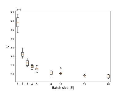
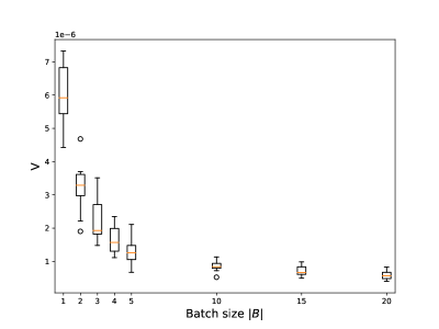
Figure 1: Variance $\mathsf{V}$ reduction of the fluctuation process with increasing mini-batch size. Left: Regression task on simulated data. $\mathsf{V}$ is an empirical estimation from $1000$ realisations of the variance of $\langle\|\cdot\|_{2},\mu_{t}^{N}\rangle$, where $N=800$ and $t=1.25$. The other parameters are $d=40$, $\alpha=0.1$, $\beta=1$, and the noise is $\varepsilon_{k}^{i}\sim\mathcal{N}(0,0.01I_{d})$. The boxplots are obtained with 10 samples of $\mathsf{V}$. Right: Classification task on MNIST dataset. $\mathsf{V}$ is an empirical estimation from $30$ realisations of the variance of $\frac{1}{N}\sum_{j=1}^{N}W^{\mathbf{o},0,j}_{k}$, where $N=10000$ and $k=3000$ ($t=0.3$). The boxplots are obtained with 10 samples of $\mathsf{V}.$

Central Limit Theorem. We focus here on the regression task. For different values of $\beta$, we plot in Figure 2 $\langle\mathsf{f}_{2},\eta_{t}^{N}\rangle$ for $0\leq t\leq 8$ (recall $\mathsf{f}_{2}(x)=|x|^{2}$), to show the agreement of $\langle\mathsf{f}_{2},\eta_{t}^{N}\rangle$ for different values of $\beta>3/4$, corresponding to the regime of (1.16), and the divergence from it when $\beta\leq 3/4$. For $\beta=3/4$, we also illustrate the regime derived in Proposition 1.1. The parameters chosen are $d=|B|=1$, $N=20000$, $\alpha=0.1$ and $\varepsilon_{k}^{i}\sim\mathcal{N}(0,0.01)$. The procedure to obtain the plots is as follows. We first compute $\langle\mathsf{f}_{2},\mu_{t}^{N}\rangle$ (we repeat this procedure 20000 times to get confidence intervals). Then, we approximate $\langle\mathsf{f}_{2},\bar{\mu}_{t}\rangle$ by $\langle\mathsf{f}_{2},\mu_{t}^{N^{\prime}}\rangle$ where $N^{\prime}=250000$. On Figure 2, we plot $\sqrt{N}(\langle\mathsf{f}_{2},\mu_{t}^{N}\rangle-\langle\mathsf{f}_{2},\mu_{t}^{N^{\prime}}\rangle)\simeq\langle\mathsf{f}_{2},\eta_{t}^{N}\rangle$ as a function of $t$.

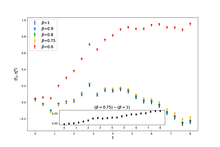
Figure 2: Time evolution of the fluctuation process for different values of $\beta$ on the regression task, with $\mathsf{f}_{2}:x\in\mathbf{R}\mapsto|x|^{2}$, $N=20000$, $d=|B|=1$, $\alpha=0.1$ and $\varepsilon_{k}^{i}\sim\mathcal{N}(0,0.01)$. Confidence intervals are obtained from $20000$ realisations. The case $\beta>3/4$ is driven by (1.16). The case $\beta=3/4$ is driven by (1.1). The case $\beta<3/4$ is not covered by our analysis. The inset exhibits the linear term in time appearing in (1.1).

Proof of Theorem 1

Pre-limit equation and remainder terms

In this section, we derive the so-called pre-limit equation (2.1.1). We then show that the remainder terms in this equation are negligible as $N\to+\infty$.

Pre-limit equation

In this section, we introduce several (random) operators acting on $\mathcal{C}^{2,\gamma_{*}}(\mathbf{R}^{d})$. Using A2 and A3, it is easy to check that all these operators belong a.s. to the dual of $\mathcal{C}^{2,\gamma_{*}}(\mathbf{R}^{d})$. The duality bracket we use in this section then is the one for the duality in $\mathcal{C}^{2,\gamma_{*}}(\mathbf{R}^{d})$. Let us consider $f\in\mathcal{C}^{2,\gamma_{*}}(\mathbf{R}^{d})$. The Taylor-Lagrange formula yields, for $N\geq 1$ and $k\in\textbf{N}$,

$$\langle f,\nu_{k+1}^{N}\rangle-\langle f,\nu_{k}^{N}\rangle =\frac{1}{N}\sum_{i=1}^{N}f(W_{k+1}^{i})-f(W_{k}^{i})$$

$$=\frac{1}{N}\sum_{i=1}^{N}\nabla f(W_{k}^{i})\cdot(W_{k+1}^{i}-W_{k}^{i})+\frac{1}{2N}\sum_{i=1}^{N}(W_{k+1}^{i}-W_{k}^{i})^{T}\nabla^{2}f(\widehat{W}_{k}^{i})(W_{k+1}^{i}-W_{k}^{i}),$$

where, for all $i\in\{1,\dots,N\}$, $\widehat{W}_{k}^{i}\in(W_{k}^{i},W_{k+1}^{i})$. Using (1.2), we have

$$\langle f,\nu_{k+1}^{N}\rangle-\langle f,\nu_{k}^{N}\rangle =\frac{1}{N}\sum_{i=1}^{N}\nabla f(W_{k}^{i})\cdot\left[\frac{\alpha}{N|B_{k}|}\sum_{(x,y)\in B_{k}}(y-g_{W^{k}}^{N}(x))\nabla_{W}\sigma_{*}(W_{k}^{i},x)+\frac{\varepsilon_{k}^{i}}{N^{\beta}}\right]+\langle f,R_{k}^{N}\rangle$$

$$=\frac{\alpha}{N|B_{k}|}\sum_{(x,y)\in B_{k}}(y-\langle\sigma_{*}(\cdot,x),\nu_{k}^{N}\rangle)\langle\nabla f\cdot\nabla\sigma_{*}(\cdot,x),\nu_{k}^{N}\rangle$$

$$\quad+\frac{1}{N^{1+\beta}}\sum_{i=1}^{N}\nabla f(W_{k}^{i})\cdot\varepsilon_{k}^{i}+\langle f,R_{k}^{N}\rangle,$$ (2.1)

where, for $N\geq 1$, $k\in\textbf{N}$ and $i=1,\dots,N$,

$$\langle f,R_{k}^{N}\rangle:=\frac{1}{2N}\sum_{i=1}^{N}(W_{k+1}^{i}-W_{k}^{i})^{T}\nabla^{2}f(\widehat{W}_{k}^{i})(W_{k+1}^{i}-W_{k}^{i}).$$ (2.2)

For $k\in\textbf{N}$, we define:

$$\langle f,D_{k}^{N}\rangle :=\frac{\alpha}{N}\int_{\mathcal{X}\times\mathcal{Y}}(y-\langle\sigma_{*}(\cdot,x),\nu_{k}^{N}\rangle\langle\nabla f\cdot\nabla\sigma_{*}(\cdot,x),\nu_{k}^{N}\rangle\pi(\mathrm{d}x,\mathrm{d}y),$$ (2.3)

$$\langle f,M_{k}^{N}\rangle :=\frac{\alpha}{N|B_{k}|}\sum_{(x,y)\in B_{k}}(y-\langle\sigma_{*}(\cdot,x),\nu_{k}^{N}\rangle)\langle\nabla f\cdot\nabla\sigma_{*}(\cdot,x),\nu_{k}^{N}\rangle-\langle f,D_{k}^{N}\rangle.$$ (2.4)

Equation (2.1.1) writes, for $k\in\textbf{N}$,

$$\langle f,\nu_{k+1}^{N}\rangle-\langle f,\nu_{k}^{N}\rangle=\langle f,D_{k}^{N}\rangle+\langle f,M_{k}^{N}\rangle+\langle f,R_{k}^{N}\rangle+\frac{1}{N^{1+\beta}}\sum_{i=1}^{N}\nabla f(W_{k}^{i})\cdot\varepsilon_{k}^{i}.$$ (2.5)

Define for $N\geq 1$ and $t\in\mathbf{R}_{+}$:

$$\langle f,D^{N}_{t}\rangle:=\sum_{k=0}^{\lfloor Nt\rfloor-1}\langle f,D_{k}^{N}\rangle\ \text{ and }\ \langle f,M^{N}_{t}\rangle:=\sum_{k=0}^{\lfloor Nt\rfloor-1}\langle f,M_{k}^{N}\rangle,$$ (2.6)

with the convention that $\sum_{0}^{-1}=0$ (which occurs if and only if $0\leq t<1/N$). It will be proved later that $\{t\mapsto\langle f,M_{t}^{N}\rangle,t\in\mathbf{R}_{+}\}$ is a martingale (see indeed Lemma 3.2), hence the notation. One has, for $t\in\mathbf{R}_{+}$,

$$\begin{split}\langle f,D^{N}_{t}\rangle&=\sum_{k=0}^{\lfloor Nt\rfloor-1}\int_{\frac{k}{N}}^{\frac{k+1}{N}}\int_{\mathcal{X}\times\mathcal{Y}}\alpha(y-\langle\sigma_{*}(\cdot,x),\nu_{k}^{N}\rangle)\langle\nabla f\cdot\nabla\sigma_{*}(\cdot,x),\nu_{k}^{N}\rangle\pi(\mathrm{d}x,\mathrm{d}y)\mathrm{d}s\\ &=\sum_{k=0}^{\lfloor Nt\rfloor-1}\int_{\frac{k}{N}}^{\frac{k+1}{N}}\int_{\mathcal{X}\times\mathcal{Y}}\alpha(y-\langle\sigma_{*}(\cdot,x),\mu_{s}^{N}\rangle)\langle\nabla f\cdot\nabla\sigma_{*}(\cdot,x),\mu_{s}^{N}\rangle\pi(\mathrm{d}x,\mathrm{d}y)\mathrm{d}s\\ &=\int_{0}^{t}\int_{\mathcal{X}\times\mathcal{Y}}\alpha(y-\langle\sigma_{*}(\cdot,x),\mu_{s}^{N}\rangle)\langle\nabla f\cdot\nabla\sigma_{*}(\cdot,x),\mu_{s}^{N}\rangle\pi(\mathrm{d}x,\mathrm{d}y)\mathrm{d}s+\langle f,V_{t}^{N}\rangle,\end{split}$$

where $\langle f,V_{t}^{N}\rangle$, for $t\in\mathbf{R}_{+}$:

$$\langle f,V_{t}^{N}\rangle:=-\int_{\frac{\lfloor Nt\rfloor}{N}}^{t}\int_{\mathcal{X}\times\mathcal{Y}}\alpha(y-\langle\sigma_{*}(\cdot,x),\mu_{s}^{N}\rangle)\langle\nabla f\cdot\nabla\sigma_{*}(\cdot,x),\mu_{s}^{N}\rangle\pi(\mathrm{d}x,\mathrm{d}y)\mathrm{d}s.$$ (2.7)

Therefore, using (2.5), we obtain that the scaled empirical measure process $\{t\mapsto\mu_{t}^{N},t\in\mathbf{R}_{+}\}$ satisfies the following pre-limit equation : for $f\in\mathcal{C}^{2,\gamma_{*}}(\mathbf{R}^{d})$, $N\geq 1$ and $t\in\mathbf{R}_{+}$,

$$\langle f,\mu_{t}^{N}\rangle-\langle f,\mu_{0}^{N}\rangle =\sum_{k=0}^{\lfloor Nt\rfloor-1}\langle f,\nu_{k+1}^{N}\rangle-\langle f,\nu_{k}^{N}\rangle$$

$$=\langle f,D^{N}_{t}\rangle+\langle f,M^{N}_{t}\rangle+\sum_{k=0}^{\lfloor Nt\rfloor-1}\langle f,R_{k}^{N}\rangle+\frac{1}{N^{1+\beta}}\sum_{k=0}^{\lfloor Nt\rfloor-1}\sum_{i=1}^{N}\nabla f(W_{k}^{i})\cdot\varepsilon_{k}^{i}$$

$$=\int_{0}^{t}\int_{\mathcal{X}\times\mathcal{Y}}\alpha(y-\langle\sigma_{*}(\cdot,x),\mu_{s}^{N}\rangle)\langle\nabla f\cdot\nabla\sigma_{*}(\cdot,x),\mu_{s}^{N}\rangle\pi(\mathrm{d}x,\mathrm{d}y)\mathrm{d}s$$

$$\quad+\langle f,M^{N}_{t}\rangle+\langle f,V_{t}^{N}\rangle+\sum_{k=0}^{\lfloor Nt\rfloor-1}\langle f,R_{k}^{N}\rangle+\frac{1}{N^{1+\beta}}\sum_{k=0}^{\lfloor Nt\rfloor-1}\sum_{i=1}^{N}\nabla f(W_{k}^{i})\cdot\varepsilon_{k}^{i}.$$ (2.8)

In the next section, we study the four last terms of (2.1.1).

The remainder terms in (2.1.1) are negligible

The aim of this section is to show that the last four terms of (2.1.1) vanish as $N\rightarrow+\infty$. This is the purpose of Lemma 2.2. The following result will be used several times in this work.

Lemma 2.1.

Let $\beta\geq 1/2$ and assume A1-A5. Then, for all $T>0$, there exists a constant $C<+\infty$ such that for all $N\geq 1,$ $i\in\{1,\dots,N\}$ and $k\in\{0,\dots,\lfloor NT\rfloor\}$,

$$\mathbf{E}\left[|W_{k}^{i}|^{8\gamma_{*}}\right]\leq C.$$

Proof.

Let us recall the following convexity inequality : for $m,p\geq 1$ and $x_{1},\dots,x_{p}\in\mathbf{R}_{+}$,

$$\Big{(}\sum_{l=1}^{m}x_{l}\Big{)}^{p}\leq m^{p-1}\sum_{l=1}^{m}x_{l}^{p}.$$ (2.9)

Let $C>0$ denotes a constant, independent of $i\in\{1,\dots,N\}$ and $0\leq k\leq\lfloor NT\rfloor$, which can change from one occurence to another. Set $p=8\gamma_{*}$. For $i\in\{1,\dots,N\}$ and $1\leq k\leq\lfloor NT\rfloor$, we have, using (1.2) and A2 :

$$|W_{k}^{i}| \leq|W_{0}^{i}|+\Big{|}\sum_{j=0}^{k-1}W_{j+1}^{i}-W_{j}^{i}\Big{|}\leq|W_{0}^{i}|+\frac{C}{N}\sum_{j=0}^{k-1}\frac{1}{|B_{j}|}\sum_{(x,y)\in B_{j}}(|y|+C)+\frac{1}{N^{\beta}}\Big{|}\sum_{j=0}^{k-1}\varepsilon_{j}^{i}\Big{|}.$$

Thus, by (2.9),

$$|W_{k}^{i}|^{p} \leq C\Big{[}|W_{0}^{i}|^{p}+\frac{1}{N}\sum_{j=0}^{k-1}\frac{1}{|B_{j}|^{p}}\Big{(}\sum_{(x,y)\in B_{j}}(|y|+C)\Big{)}^{p}+\frac{1}{N^{p\beta}}\Big{|}\sum_{j=0}^{k-1}\varepsilon_{j}^{i}\Big{|}^{p}\Big{]}$$

$$\leq C\Big{[}|W_{0}^{i}|^{p}+\frac{1}{N}\sum_{j=0}^{k-1}\frac{1}{|B_{j}|}\sum_{(x,y)\in B_{j}}(|y|+C)^{p}+\frac{1}{N^{p\beta}}\Big{|}\sum_{j=0}^{k-1}\varepsilon_{j}^{i}\Big{|}^{p}\Big{]}.$$

We have:

$$\textbf{E}\Big{[}\frac{1}{|B_{j}|}\sum_{(x,y)\in B_{j}}(|y|+C)^{p}\Big{]} \leq C\Big{[}\textbf{E}\Big{[}\frac{1}{|B_{j}|}\sum_{n=1}^{|B_{j}|}|y_{j}^{n}|^{p}\Big{]}+1\Big{]},$$

and, using A1 and (A3), it holds for $j\geq 0$:

$$\textbf{E}\Big{[}\frac{1}{|B_{j}|}\sum_{n=1}^{|B_{j}|}|y_{j}^{n}|^{p}\Big{]}=\sum_{q=1}^{+\infty}\,\textbf{E}\Big{[}\frac{\mathbf{1}_{|B_{j}|=q}}{q}\,\sum_{n=1}^{q}|y_{j}^{n}|^{p}\Big{]} =\sum_{q=1}^{+\infty}\,\frac{1}{q}\,\sum_{n=1}^{q}\,\textbf{E}\big{[}|y_{j}^{n}|^{p}\mathbf{1}_{|B_{j}|=q}\big{]}$$

$$=\sum_{q=1}^{+\infty}\,\frac{1}{q}\,\sum_{n=1}^{q}\,\textbf{E}\big{[}|y_{j}^{n}|^{p}\big{]}\,\textbf{E}\big{[}\mathbf{1}_{|B_{j}|=q}\big{]}$$

$$=\textbf{E}\big{[}|y_{1}^{1}|^{p}\big{]}<+\infty.$$ (2.10)

Thus, using the two previous inequalities, we deduce that:

$$\textbf{E}\Big{[}\frac{1}{N}\sum_{j=0}^{k-1}\frac{1}{|B_{j}|}\sum_{(x,y)\in B_{j}}(|y|+C)^{p}\Big{]}\leq C.$$

By A4, $\textbf{E}\left[|W_{0}^{i}|^{p}\right]\leq C$. In addition, we have that, for $i\in\{1,\dots,N\}$,

$$\Big{|}\sum_{j=0}^{k-1}\varepsilon_{j}^{i}\Big{|}^{p}\leq C\sum_{l=1}^{d}\Big{|}\sum_{j=0}^{k-1}\varepsilon_{j}^{i,l}\Big{|}^{p}$$

Since we deal with the sum of centered independent Gaussian random variables, we have that, for all $i\in\{1,\dots,N\}$ and $l\in\{1,\dots,d\}$,

$$\textbf{E}\Big{[}\Big{|}\sum_{j=0}^{k-1}\varepsilon_{j}^{i,l}\Big{|}^{p}\Big{]}\leq Ck^{p/2}\leq CN^{p/2}.$$

Putting all these inequalities together, we obtain that $\textbf{E}\left[|W_{k}^{i}|^{p}\right]\leq C\left[1+\frac{N^{p/2}}{N^{p\beta}}\right]\leq C$ (recall $\beta\geq 1/2)$. This concludes the proof of the lemma. ∎

Lemma 2.2.

Let $\beta\geq 1/2$ and assume A1-A5. Then, for all $T>0$ there exists $C<\infty$ such that for all $N\geq 1$ and $f\in\mathcal{C}^{2,\gamma_{*}}(\mathbf{R}^{d})$,

1. $\max_{0\leq k<\lfloor NT\rfloor}\mathbf{E}\left[|\langle f,R_{k}^{N}\rangle|\right]\leq C\|f\|_{\mathcal{C}^{2,\gamma_{*}}}\left[\frac{1}{N^{2}}+\frac{1}{N^{2\beta}}\right]$.

2. $\sup_{t\in[0,T]}\mathbf{E}\left[|\langle f,V_{t}^{N}\rangle|\right]\leq{C\|f\|_{\mathcal{C}^{2,\gamma_{*}}}}/{N}$.

3. $\sup_{t\in[0,T]}\mathbf{E}\left[|\langle f,M_{t}^{N}\rangle|^{2}\right]\leq{C\|f\|_{\mathcal{C}^{2,\gamma_{*}}}^{2}}/{N}$.

4. $\sup_{t\in[0,T]}\mathbf{E}\left[\left|\frac{1}{N^{1+\beta}}\sum_{k=0}^{\lfloor Nt\rfloor-1}\sum_{i=1}^{N}\nabla f(W_{k}^{i})\cdot\varepsilon_{k}^{i}\right|^{2}\right]\leq{C\|f\|_{\mathcal{C}^{2,\gamma_{*}}}^{2}}/{N^{2\beta}}$.

Proof.

Let $T>0$ and $f\in\mathcal{C}^{2,\gamma_{*}}(\mathbf{R}^{d})$. In what follows, $C>0$ is a constant, independent of $N\geq 1$, $t\in[0,T]$, $f$, and $k\in\{0,\dots,\lfloor NT\rfloor-1\}$, which can change from one line to another.

Proof of item (i). For $k\in\{0,\dots,\lfloor NT\rfloor-1\}$, by (2.2), we have

$$|\langle f,R_{k}^{N}\rangle|\leq\frac{C\|f\|_{\mathcal{C}^{2,\gamma_{*}}}}{N}\sum_{i=1}^{N}|W_{k+1}^{i}-W_{k}^{i}|^{2}(1+|\widehat{W}_{k}^{i}|^{\gamma_{*}}).$$ (2.11)

On the other hand, by (1.2), we have:

$$|W_{k+1}^{i}-W_{k}^{i}|\leq\frac{C}{N|B_{k}|}\sum_{(x,y)\in B_{k}}\big{(}|y|+|g_{W_{k}}^{N}(x)|\big{)}+\frac{|\varepsilon_{k}^{i}|}{N^{\beta}}.$$ (2.12)

By (2.9) and the triangle inequality, we deduce

$$|W_{k+1}^{i}-W_{k}^{i}|^{2}\leq C\Big{[}\frac{1}{N^{2}|B_{k}|}\sum_{(x,y)\in B_{k}}(|y|^{2}+|g_{W_{k}}^{N}(x)|^{2})+\frac{|\varepsilon_{k}^{i}|^{2}}{N^{2\beta}}\Big{]}.$$

By definition of $\widehat{W}_{k}^{i}$, there exists $\alpha_{k}^{i}\in(0,1)$ such that $\widehat{W}_{k}^{i}=\alpha_{k}^{i}W_{k}^{i}+(1-\alpha_{k}^{i})W_{k+1}^{i}$, leading, by (2.9), to $|\widehat{W}_{k}^{i}|^{\gamma_{*}}\leq C\left[|W_{k}^{i}|^{\gamma_{*}}+|W_{k+1}^{i}|^{\gamma_{*}}\right]$. Therefore,

$$|W_{k+1}^{i}-W_{k}^{i}|^{2}(1+|\widehat{W}_{k}^{i}|^{\gamma_{*}}) \leq C\Big{[}\frac{1}{N^{2}|B_{k}|}\sum_{(x,y)\in B_{k}}(|y|^{2}+|g_{W_{k}}^{N}(x)|^{2})+\frac{|\varepsilon_{k}^{i}|^{2}}{N^{2\beta}}\Big{]}(1+|W_{k}^{i}|^{\gamma_{*}}+|W_{k+1}^{i}|^{\gamma_{*}})$$

$$\leq\frac{C}{N^{2}}(1+|W_{k}^{i}|^{\gamma_{*}}+|W_{k+1}^{i}|^{\gamma_{*}})^{2}+\frac{C}{N^{2}|B_{k}|}\sum_{(x,y)\in B_{k}}(|y|^{4}+|g_{W_{k}}(x)|^{4})$$

$$\quad+\frac{C}{N^{2\beta}}\left[|\varepsilon_{k}^{i}|^{4}+(1+|W_{k}^{i}|^{\gamma_{*}}+|W_{k+1}^{i}|^{\gamma_{*}})^{2}\right].$$ (2.13)

Plugging (2.13) in (2.11), we obtain

$$|\langle f,R_{k}^{N}\rangle| \leq\frac{C\|f\|_{\mathcal{C}^{2,\gamma_{*}}}}{N}\sum_{i=1}^{N}\Big{[}\frac{1}{N^{2}}(1+|W_{k}^{i}|^{\gamma_{*}}+|W_{k+1}^{i}|^{\gamma_{*}})^{2}+\frac{1}{N^{2}|B_{k}|}\sum_{(x,y)\in B_{k}}(|y|^{4}+C)$$

$$\quad+\frac{1}{N^{2\beta}}\left[|\varepsilon_{k}^{i}|^{4}+(1+|W_{k}^{i}|^{\gamma_{*}}+|W_{k+1}^{i}|^{\gamma_{*}})^{2}\right]\Big{]}.$$ (2.14)

Finally, using Lemma 2.1, A3, and A5, one deduces that $\textbf{E}\left[|\langle f,R_{k}^{N}\rangle|\right]\leq C\|f\|_{\mathcal{C}^{2,\gamma_{*}}}({1}/{N^{2}}+{1}/{N^{2\beta}})$. This proves item (i).

Proof of item (ii). Let $t\in[0,T]$. Since $\sigma_{*}$ and all its derivatives are bounded (see A2), it holds for all $s\geq 0$:

$$|\langle\sigma_{*}(\cdot,x),\mu_{s}^{N}\rangle|=\Big{|}\frac{1}{N}\sum_{i=1}^{N}\sigma_{*}(W_{\lfloor Ns\rfloor}^{i},x)\Big{|}\leq C,$$ (2.15)

and

$$|\langle\nabla f\cdot\nabla\sigma_{*}(\cdot,x),\mu_{s}^{N}\rangle| =\Big{|}\frac{1}{N}\sum_{i=1}^{N}\nabla f(W_{\lfloor Ns\rfloor}^{i})\cdot\nabla_{W}\sigma_{*}(W_{\lfloor Ns\rfloor}^{i},x)\Big{|}\leq\frac{C\|f\|_{\mathcal{C}^{2,\gamma_{*}}}}{N}\sum_{i=1}^{N}(1+|W_{\lfloor Ns\rfloor}^{i}|^{\gamma_{*}}).$$ (2.16)

Notice that $C$ above is also independent of $x\in\mathcal{X}$. Since $\mathbf{E}[|y|]<+\infty$ (see (A3)), we obtain

$$\left|\int_{\mathcal{X}\times\mathcal{Y}}\alpha(y-\langle\sigma_{*}(\cdot,x),\mu_{s}^{N}\rangle)\langle\nabla f\cdot\nabla\sigma_{*}(\cdot,x),\mu_{s}^{N}\rangle\pi(\mathrm{d}x,\mathrm{d}y)\right|\leq\frac{C\|f\|_{\mathcal{C}^{2,\gamma_{*}}}}{N}\sum_{i=1}^{N}(1+|W_{\lfloor Ns\rfloor}^{i}|^{\gamma_{*}}).$$ (2.17)

Noticing that $s\in(\frac{\lfloor Nt\rfloor}{N},t)\Rightarrow\lfloor Ns\rfloor=\lfloor Nt\rfloor$, we obtain (see (2.7))

$$|\langle f,V_{t}^{N}\rangle|\leq\left(t-\frac{\lfloor Nt\rfloor}{N}\right)\frac{C\|f\|_{\mathcal{C}^{2,\gamma_{*}}}}{N}\sum_{i=1}^{N}(1+|W_{\lfloor Nt\rfloor}^{i}|^{\gamma_{*}}).$$ (2.18)

Then, by Lemma 2.1, $\textbf{E}\left[|\langle f,V_{t}^{N}\rangle|\right]\leq{C\|f\|_{\mathcal{C}^{2,\gamma_{*}}}}/{N}$. This proves item (ii).

Proof of item (iii). Let $t\in[0,T]$. Recall the definition of $\mathcal{F}_{k}^{N}$ in (1.9) and $\langle f,M_{k}^{N}\rangle$ in (2.4).

Step 1. In this step we prove that

$$\textbf{E}\left[|\langle f,M_{k}^{N}\rangle|^{2}\right]\leq{C\|f\|_{\mathcal{C}^{2,\gamma_{*}}}^{2}}/{N^{2}}.$$ (2.19)

With the same arguments as those used to get (2.15) and (2.16), we have

$$|\langle\sigma_{*}(\cdot,x),\nu_{k}^{N}\rangle|\leq C\quad\text{and}\quad|\langle\nabla f\cdot\nabla\sigma_{*}(\cdot,x),\nu_{k}^{N}\rangle|\leq\frac{C\|f\|_{\mathcal{C}^{2,\gamma_{*}}}}{N}\sum_{i=1}^{N}(1+|W_{k}^{i}|^{\gamma_{*}}).$$ (2.20)

Note that $C$ above is also independent of $x\in\mathcal{X}$. By (2.9) and (2.20), we have:

$$|\langle f,M_{k}^{N}\rangle|^{2} \leq\frac{C}{N^{2}|B_{k}|}\sum_{(x,y)\in B_{k}}(y-\langle\sigma_{*}(\cdot,x),\nu_{k}^{N}\rangle)^{2}\langle\nabla f\cdot\nabla\sigma_{*}(\cdot,x),\nu_{k}^{N}\rangle^{2}+C|\langle f,D_{k}^{N}\rangle|^{2}$$

$$\leq\frac{C}{N^{2}|B_{k}|}\sum_{(x,y)\in B_{k}}(|y|^{2}+C)\langle\nabla f\cdot\nabla\sigma_{*}(\cdot,x),\nu_{k}^{N}\rangle^{2}+C|\langle f,D_{k}^{N}\rangle|^{2}$$

$$\leq\frac{C\|f\|_{\mathcal{C}^{2,\gamma_{*}}}^{2}}{N^{3}|B_{k}|}\sum_{(x,y)\in B_{k}}(|y|^{2}+C)\sum_{i=1}^{N}(1+|W_{k}^{i}|^{\gamma_{*}})^{2}+C|\langle f,D_{k}^{N}\rangle|^{2}.$$ (2.21)

On the other hand, it holds since $(W_{k}^{1},\dots,W_{k}^{N})$ is $\mathcal{F}_{k}^{N}$-measurable and by A1:

$$\mathbf{E}\Big{[}\frac{1}{|B_{k}|}\sum_{(x,y)\in B_{k}}(|y|^{2}+C)\sum_{i=1}^{N}(1+|W_{k}^{i}|^{\gamma_{*}})^{2}\Big{]} =\sum_{q\geq 1}\,\frac{1}{q}\,\mathbf{E}\Big{[}\mathbf{1}_{|B_{k}|=q}\sum_{n=1}^{q}(|y_{k}^{n}|^{2}+C)\sum_{i=1}^{N}(1+|W_{k}^{i}|^{\gamma_{*}})^{2}\Big{]}$$

$$=\sum_{q\geq 1}\,\frac{1}{q}\,\mathbf{E}\Big{[}\mathbf{1}_{|B_{k}|=q}\sum_{n=1}^{q}(|y_{k}^{n}|^{2}+C)\Big{]}\mathbf{E}\Big{[}\sum_{i=1}^{N}(1+|W_{k}^{i}|^{\gamma_{*}})^{2}\Big{]}$$

$$=\sum_{q\geq 1}\,\frac{1}{q}\,\mathbf{E}\Big{[}\mathbf{1}_{|B_{k}|=q}\Big{]}\mathbf{E}\Big{[}\sum_{n=1}^{q}(|y_{k}^{n}|^{2}+C)\Big{]}\mathbf{E}\Big{[}\sum_{i=1}^{N}(1+|W_{k}^{i}|^{\gamma_{*}})^{2}\Big{]}$$

$$=\sum_{q\geq 1}\mathbf{E}\Big{[}\mathbf{1}_{|B_{k}|=q}\Big{]}\mathbf{E}\Big{[}|y_{1}^{1}|^{2}+C\Big{]}\mathbf{E}\Big{[}\sum_{i=1}^{N}(1+|W_{k}^{i}|^{\gamma_{*}})^{2}\Big{]}$$

$$=\mathbf{E}\Big{[}|y_{1}^{1}|^{2}+C\Big{]}\mathbf{E}\Big{[}\sum_{i=1}^{N}(1+|W_{k}^{i}|^{\gamma_{*}})^{2}\Big{]}\leq CN,$$ (2.22)

where we have used Lemma 2.1 and A3 for the last inequality. Consequently, one has:

$$\textbf{E}\left[|\langle f,M_{k}^{N}\rangle|^{2}\right]\leq\frac{C\|f\|_{\mathcal{C}^{2,\gamma_{*}}}^{2}}{N^{2}}+C\textbf{E}\left[\langle f,D_{k}^{N}\rangle^{2}\right].$$ (2.23)

On the other hand, we easily obtain with similar arguments that $\textbf{E}\left[|\langle f,D_{k}^{N}\rangle|^{2}\right]\leq{C\|f\|_{\mathcal{C}^{2,\gamma_{*}}}^{2}}/{N^{2}}$. Together with (2.23), this ends the proof of (2.19).

Step 2. In this step we prove that for all $k\geq 0$:

$$\textbf{E}\left[\langle f,M_{k}^{N}\rangle|\mathcal{F}_{k}^{N}\right]=0.$$ (2.24)

For ease of notation, we set

$$\mathrm{Q}^{N}[f](x,y,\{W_{k}^{i}\}_{i=1,\ldots,N})=\big{(}y-\langle\sigma_{*}(\cdot,x),\nu_{k}^{N}\rangle\big{)}\langle\nabla f\cdot\nabla\sigma_{*}(\cdot,x),\nu_{k}^{N}\rangle.$$ (2.25)

With this notation, we have (see (2.3)) $\langle f,D_{k}^{N}\rangle=\frac{\alpha}{N}\int_{\mathcal{X}\times\mathcal{Y}}\mathrm{Q}^{N}[f](x,y,\{W_{k}^{i}\}_{i=1,\ldots,N})\pi(\mathrm{d}x,\mathrm{d}y)$ and $\langle f,M_{k}^{N}\rangle=\frac{\alpha}{N|B_{k}|}\sum_{(x,y)\in B_{k}}\mathrm{Q}^{N}[f](x,y,\{W_{k}^{i}\}_{i=1,\ldots,N})-\langle f,D_{k}^{N}\rangle$. It then holds:

$$\mathbf{E}\Big{[}\frac{1}{|B_{k}|}\sum_{(x,y)\in B_{k}}\mathrm{Q}^{N}[f](x,y,\{W_{k}^{i}\}_{i=1,\ldots,N})\,\big{|}\,\mathcal{F}_{k}^{N}\Big{]} =\mathbf{E}\Big{[}\frac{1}{|B_{k}|}\sum_{n=1}^{|B_{k}|}\mathrm{Q}^{N}[f](x_{k}^{n},y_{k}^{n},\{W_{k}^{i}\}_{i=1,\ldots,N})\,\big{|}\,\mathcal{F}_{k}^{N}\Big{]}$$

$$=\sum_{q\geq 1}\frac{1}{q}\mathbf{E}\Big{[}\mathbf{1}_{|B_{k}|=q}\sum_{n=1}^{q}\mathrm{Q}^{N}[f](x_{k}^{n},y_{k}^{n},\{W_{k}^{i}\}_{i=1,\ldots,N})\,\big{|}\,\mathcal{F}_{k}^{N}\Big{]}.$$

Since $(W_{k}^{1},\dots,W_{k}^{N})$ is $\mathcal{F}_{k}^{N}$-measurable, $\big{(}|B_{k}|,((x_{k}^{n},y_{k}^{n}))_{n\geq 1}\big{)}\perp\!\!\!\perp\mathcal{F}_{k}^{N}$, and $|B_{k}|\perp\!\!\!\perp((x_{k}^{n},y_{k}^{n}))_{n\geq 1}$ (see A1), we deduce that

$$\mathbf{E}\Big{[}\mathbf{1}_{|B_{k}|=q}\sum_{n=1}^{q}\mathrm{Q}^{N}[f](x_{k}^{n},y_{k}^{n},\{W_{k}^{i}\}_{i=1,\ldots,N})\,\big{|}\,\mathcal{F}_{k}^{N}\Big{]}$$

$$=\mathbf{E}\Big{[}\mathbf{1}_{|B_{k}|=q}\sum_{n=1}^{q}\mathrm{Q}^{N}[f](x_{k}^{n},y_{k}^{n},\{w_{k}^{i}\}_{i=1,\ldots,N})\Big{]}\Big{|}_{\{w_{k}^{i}\}_{i}=\{W_{k}^{i}\}_{i}}$$

$$=\mathbf{E}\big{[}\mathbf{1}_{|B_{k}|=q}\big{]}\mathbf{E}\Big{[}\sum_{n=1}^{q}\mathrm{Q}^{N}[f](x_{k}^{n},y_{k}^{n},\{w_{k}^{i}\}_{i=1,\ldots,N})\Big{]}\Big{|}_{\{w_{k}^{i}\}_{i}=\{W_{k}^{i}\}_{i}}$$

$$=q\mathbf{E}\big{[}\mathbf{1}_{|B_{k}|=q}\big{]}\mathbf{E}\Big{[}\mathrm{Q}^{N}[f](x_{1}^{1},y_{1}^{1},\{w_{k}^{i}\}_{i=1,\ldots,N})\Big{]}\Big{|}_{\{w_{k}^{i}\}_{i}=\{W_{k}^{i}\}_{i}}$$

$$=q\,\frac{N}{\alpha}\mathbf{E}\big{[}\mathbf{1}_{|B_{k}|=q}\big{]}\,\langle f,D_{k}^{N}\rangle,$$

where we have used A3 to deduce the last two equalities. We have thus proved that

$$\mathbf{E}\Big{[}\frac{\alpha}{N|B_{k}|}\sum_{(x,y)\in B_{k}}\mathrm{Q}^{N}[f](x_{k}^{n},y_{k}^{n},\{W_{k}^{i}\}_{i=1,\ldots,N})\,\big{|}\,\mathcal{F}_{k}^{N}\Big{]}=\langle f,D_{k}^{N}\rangle.$$

Therefore, using in addition that $\mathbf{E}[\langle f,D_{k}^{N}\rangle|\,\mathcal{F}_{k}^{N}]=\langle f,D_{k}^{N}\rangle$ (because $(W_{k}^{1},\dots,W_{k}^{N})$ is $\mathcal{F}_{k}^{N}$-measurable), we finally deduce (2.24).

Step 3. We now end the proof of item (iii). If $j>k$, $\langle f,M_{k}^{N}\rangle$ is $\mathcal{F}_{j}^{N}$-measurable (because $\langle f,M_{k}^{N}\rangle$ is $\mathcal{F}_{k+1}^{N}$-measurable). Then, using also (2.24), one obtains that for $j>k$:

$$\textbf{E}\left[\langle f,M_{k}^{N}\rangle\langle f,M_{j}^{N}\rangle\right]=\textbf{E}\left[\langle f,M_{k}^{N}\rangle\textbf{E}\left[\langle f,M_{j}^{N}\rangle|\mathcal{F}_{j}^{N}\right]\right]=\textbf{E}\left[\langle f,M_{k}^{N}\rangle\times 0\right]=0.$$ (2.26)

We then have (see (2.6)):

$$\textbf{E}\left[|\langle f,M^{N}_{t}\rangle|^{2}\right] =\sum_{k=0}^{\lfloor Nt\rfloor-1}\textbf{E}\left[|\langle f,M_{k}^{N}\rangle|^{2}\right].$$ (2.27)

Plugging (2.19) in (2.27) implies item (iii).

Proof of item (iv). Let $t\in[0,T]$. By Lemma 2.1, $\nabla f(W_{k}^{i})\cdot\varepsilon_{k}^{i}$ is square-integrable for all $k\in\mathbf{N}$ and $i\in\{1,\ldots,N\}$. From the equality

$$\textbf{E}\Big{[}\Big{|}\sum_{k=0}^{\lfloor Nt\rfloor-1}\sum_{i=1}^{N}\nabla f(W_{k}^{i})\cdot\varepsilon_{k}^{i}\Big{|}^{2}\Big{]}=\sum_{j,k=0}^{\lfloor Nt\rfloor-1}\sum_{i,\ell=1}^{N}\textbf{E}\big{[}\nabla f(W_{k}^{i})\cdot\varepsilon_{k}^{i}\,\nabla f(W_{j}^{\ell})\cdot\varepsilon_{j}^{\ell}\big{]}.$$

Recall that $W_{a}^{b}$ is $\mathcal{F}_{a}^{N}$-measurable for all $a\in\mathbf{N}$ and $b\in\{1,\ldots,N\}$, and that $\varepsilon_{a}^{b}\perp\!\!\!\perp\mathcal{F}_{a}^{N}$ (see A5). Let $e_{q}$ denotes the $q$-th element of the canonical basis of $\mathbf{R}^{d}$ ($q\in\{1,\ldots,d\})$. Assume that $0\leq j<k\leq\lfloor Nt\rfloor-1$. Then, $\varepsilon_{j}^{\ell}$ is $\mathcal{F}_{k}^{N}$-measurable, and it holds for all $i,\ell\in\{1,\ldots,N\}$:

$$\textbf{E}\big{[}\nabla f(W_{k}^{i})\cdot\varepsilon_{k}^{i}\,\nabla f(W_{j}^{\ell})\cdot\varepsilon_{j}^{\ell}\big{]}=\sum_{n,m=1}^{d}\textbf{E}\Big{[}\partial_{e_{n}}f(W_{k}^{i})\,\partial_{e_{m}}f(W_{j}^{\ell})\,\varepsilon_{j}^{\ell}\cdot e_{m}\Big{]}\mathbf{E}\big{[}\varepsilon_{k}^{i}\cdot e_{n}\big{]}=0.$$ (2.28)

because $\varepsilon_{k}^{i}\sim\mathcal{N}(0,I_{d})$ (see A5). On the other hand, using A5, we have for all $0\leq k\leq\lfloor Nt\rfloor-1$ and when $i\neq\ell\in\{1,\ldots,N\}$:

$$\textbf{E}\big{[}\nabla f(W_{k}^{i})\cdot\varepsilon_{k}^{i}\,\nabla f(W_{k}^{\ell})\cdot\varepsilon_{k}^{\ell}\big{]} =\sum_{n,m=1}^{d}\textbf{E}\Big{[}\,\partial_{e_{n}}f(W_{k}^{i})\,\partial_{e_{m}}f(W_{k}^{\ell})\,\Big{]}\mathbf{E}\big{[}\varepsilon_{k}^{i}\cdot e_{n}\big{]}\mathbf{E}\big{[}\varepsilon_{k}^{\ell}\cdot e_{m}\big{]}=0.$$ (2.29)

Consequently, we have:

$$\textbf{E}\Big{[}\Big{|}\sum_{k=0}^{\lfloor Nt\rfloor-1}\sum_{i=1}^{N}\nabla f(W_{k}^{i})\cdot\varepsilon_{k}^{i}\Big{|}^{2}\Big{]}=\sum_{k=0}^{\lfloor Nt\rfloor-1}\sum_{i=1}^{N}\textbf{E}\big{[}|\nabla f(W_{k}^{i})\cdot\varepsilon_{k}^{i}|^{2}\big{]}.$$

Using the Cauchy-Schwarz inequality, we deduce, using also Lemma 2.1 and A5, that:

$$\textbf{E}\Big{[}\Big{|}\sum_{k=0}^{\lfloor Nt\rfloor-1}\sum_{i=1}^{N}\nabla f(W_{k}^{i})\cdot\varepsilon_{k}^{i}\Big{|}^{2}\Big{]} \leq\sum_{k=0}^{\lfloor Nt\rfloor-1}\sum_{i=1}^{N}\textbf{E}\left[|\nabla f(W_{k}^{i})|^{2}\right]\textbf{E}\left[|\varepsilon_{k}^{i}|^{2}\right]$$

$$\leq C\|f\|_{\mathcal{C}^{2,\gamma_{*}}}^{2}\sum_{k=0}^{\lfloor Nt\rfloor-1}\sum_{i=1}^{N}\textbf{E}\left[(1+|W_{k}^{i}|^{\gamma_{*}})^{2}\right]\leq C\|f\|_{\mathcal{C}^{2,\gamma_{*}}}^{2}N^{2}.$$ (2.30)

This proves (iv). The proof of Lemma 2.2 is complete. ∎

We now want to pass to the limit in (2.1.1). To this end, we first prove that $(\mu^{N})_{N\geq 1}$ is relatively compact in $\mathcal{D}(\mathbf{R}_{+},\mathcal{H}^{-L,\gamma}(\mathbf{R}^{d}))$. This is the purpose of the following section.

Relative compactness in $\mathcal{D}(\mathbf{R}_{+},\mathcal{P}_{\gamma}(\mathbf{R}^{d}))$ and convergence to the limit equation

In this section, we show that $(\mu^{N})_{N\geq 1}$ is relatively compact in $\mathcal{D}(\mathbf{R}_{+},\mathcal{P}_{\gamma}(\mathbf{R}^{d}))$. Then, we prove that any limit point of $(\mu^{N})_{N\geq 1}$ satisfies a.s. (1.10).

Relative compactness in $\mathcal{D}(\mathbf{R}_{+},\mathcal{P}_{\gamma}(\mathbf{R}^{d}))$

In this section we prove the following result.

Proposition 2.3.

Let $\beta\geq 1/2$ and assume that the conditions A1-A5 hold. Then, $(\mu^{N})_{N\geq 1}$ is relatively compact in in $\mathcal{D}(\mathbf{R}_{+},\mathcal{P}_{\gamma}(\mathbf{R}^{d}))$.

We first recall the following standard result.

Proposition 2.4.

Let $q>p\geq 1$ and $C>0$. The set $\mathscr{K}_{C}^{q}:=\{\mu\in\mathcal{P}_{p}(\mathbf{R}^{d}),\int_{\mathbf{R}^{d}}|x|^{q}\mu(\mathrm{d}x)\leq C\}$ is compact.

We have the following result.

Lemma 2.5.

Let $\beta\geq 1/2$ and assume that A1-A5 hold. Then, for every $T>0$, there exists $C>0$ such that for all $f\in\mathcal{C}^{2,\gamma_{*}}(\mathbf{R}^{d})$,

$$\sup_{N\geq 1}\mathbf{E}\Big{[}\sup_{t\in[0,T]}\langle f,\mu_{t}^{N}\rangle^{2}\Big{]}\leq C\|f\|_{\mathcal{C}^{2,\gamma_{*}}}^{2}.$$ (2.31)

Proof.

Let $T>0$ and $f\in\mathcal{C}^{2,\gamma_{*}}(\mathbf{R}^{d})$. All along the proof, $C<\infty$ denotes a constant independent of $t\in[0,T]$, $N\geq 1$, $k\in\{0,\ldots,\lfloor Nt\rfloor\}$, $i\in\{1,\ldots,N\}$, and $f\in\mathcal{C}^{2,\gamma_{*}}(\mathbf{R}^{d})$, which can change from one occurence to another. From (2.1.1), we have:

$$\sup_{t\in[0,T]}\langle f,\mu_{t}^{N}\rangle^{2} \leq C\Big{[}\langle f,\mu_{0}^{N}\rangle^{2}+\int_{0}^{T}\int_{\mathcal{X}\times\mathcal{Y}}(y-\langle\sigma_{*}(\cdot,x),\mu_{s}^{N}\rangle)^{2}\langle\nabla f\cdot\nabla\sigma_{*}(\cdot,x),\mu_{s}^{N}\rangle^{2}\pi(\mathrm{d}x,\mathrm{d}y)\mathrm{d}s$$

$$\quad+\sup_{t\in[0,T]}\langle f,M^{N}_{t}\rangle^{2}+\sup_{t\in[0,T]}|\langle f,V_{t}^{N}\rangle|^{2}+\sup_{t\in[0,T]}\Big{|}\sum_{k=0}^{\lfloor Nt\rfloor-1}\langle f,R_{k}^{N}\rangle\Big{|}^{2}$$

$$\quad+\frac{1}{N^{2+2\beta}}\sup_{t\in[0,T]}\Big{|}\sum_{k=0}^{\lfloor Nt\rfloor-1}\sum_{i=1}^{N}\nabla f(W_{k}^{i})\cdot\varepsilon_{k}^{i}\Big{|}^{2}\,\Big{]}.$$ (2.32)

We now study each term of the right-hand side of (2.2.1). Let us deal with the first term in the right-hand side of (2.2.1). Using A4 and (2.9), it holds:

$$\textbf{E}\left[\langle f,\mu_{0}^{N}\rangle^{2}\right]=\textbf{E}\left[\langle f,\nu_{0}^{N}\rangle^{2}\right]=\textbf{E}\Big{[}\Big{|}\frac{1}{N}\sum_{i=1}^{N}f(W_{0}^{i})\Big{|}^{2}\Big{]}\leq\frac{1}{N}\sum_{i=1}^{N}\textbf{E}\left[|f(W_{0}^{i})|^{2}\right] \leq\frac{\|f\|^{2}_{\mathcal{C}^{2,\gamma_{*}}}}{N}\sum_{i=1}^{N}\textbf{E}\left[(1+|W_{0}^{i}|^{\gamma_{*}})^{2}\right]$$

$$\leq C\|f\|^{2}_{\mathcal{C}^{2,\gamma_{*}}}.$$

For the second term in the right-hand side of (2.2.1), we have since $\mathbf{E}[|y|^{2}]<+\infty$ (see (A3)) and using (2.15), (2.16), and Lemma 2.1:

$$\textbf{E}\left[\int_{0}^{T}\int_{\mathcal{X}\times\mathcal{Y}}(y-\langle\sigma_{*}(\cdot,x),\mu_{s}^{N}\rangle)^{2}\langle\nabla f\cdot\nabla\sigma_{*}(\cdot,x),\mu_{s}^{N}\rangle^{2}\pi(\mathrm{d}x,\mathrm{d}y)\mathrm{d}s\right]\leq C\|f\|^{2}_{\mathcal{C}^{2,\gamma_{*}}}.$$

Let us deal with the third term in the right-hand side of (2.2.1). By (2.6) and (2.9), we have, for $t\in[0,T]$,

$$\sup_{t\in[0,T]}|\langle f,M_{t}^{N}\rangle|^{2}\leq\lfloor NT\rfloor\sum_{k=0}^{\lfloor NT\rfloor-1}\langle f,M_{k}^{N}\rangle^{2}.$$

Hence, using (2.19), we obtain that $\textbf{E}\big{[}\sup_{t\in[0,T]}\langle f,M_{t}^{N}\rangle^{2}\big{]}\leq C\|f\|_{\mathcal{C}^{2,\gamma_{*}}}^{2}$. Let us deal with the fourth term in the right-hand side of (2.2.1). From (2.9) and (2.18),

$$\sup_{t\in[0,T]}|\langle f,V_{t}^{N}\rangle|^{2}\leq\frac{C\|f\|_{\mathcal{C}^{2,\gamma_{*}}}^{2}}{N^{3}}\sum_{i=1}^{N}\max_{0\leq k\leq\lfloor NT\rfloor}(1+|W_{k}^{i}|^{\gamma_{*}})^{2},$$

which leads to

$$\textbf{E}\Big{[}\sup_{t\in[0,T]}|\langle f,V_{t}^{N}\rangle|^{2}\Big{]} \leq\frac{C\|f\|_{\mathcal{C}^{2,\gamma_{*}}}^{2}}{N^{3}}\sum_{i=1}^{N}\textbf{E}\left[\max_{0\leq k\leq\lfloor NT\rfloor}(1+|W_{k}^{i}|^{\gamma_{*}})^{2}\right]$$

$$\leq\frac{C\|f\|_{\mathcal{C}^{2,\gamma_{*}}}^{2}}{N^{3}}\sum_{i=1}^{N}\sqrt{\sum_{k=0}^{\lfloor NT\rfloor}\textbf{E}\left[(1+|W_{k}^{i}|^{\gamma_{*}})^{4}\right]}\leq\frac{C\|f\|_{\mathcal{C}^{2,\gamma_{*}}}^{2}}{N^{3/2}}.$$ (2.33)

Let us now consider the fifth term in the right-hand side of (2.2.1). From (2.1.2) and (2.9), we have

$$|\langle f,R_{k}^{N}\rangle|^{2} \leq\frac{C\|f\|^{2}_{\mathcal{C}^{2,\gamma_{*}}}}{N}\sum_{i=1}^{N}\Big{[}\frac{1}{N^{4}}(1+|W_{k}^{i}|^{\gamma_{*}}+|W_{k+1}^{i}|^{\gamma_{*}})^{4}+\frac{1}{N^{4}|B_{k}|}\sum_{(x,y)\in B_{k}}(|y|^{4}+C)^{2}$$

$$\quad+\frac{1}{N^{4\beta}}\left[|\varepsilon_{k}^{i}|^{8}+(1+|W_{k}^{i}|^{\gamma_{*}}+|W_{k+1}^{i}|^{\gamma_{*}})^{4}\right]\Big{]}.$$

Then, by A3 and A5 together with Lemma 2.1 and (2.10), we obtain

$$\textbf{E}\left[|\langle f,R_{k}^{N}\rangle|^{2}\right]\leq C\|f\|^{2}_{\mathcal{C}^{2,\gamma_{*}}}\Big{[}\frac{1}{N^{4}}+\frac{1}{N^{4\beta}}\Big{]}.$$ (2.34)

Therefore, using also (2.9), it holds:

$$\textbf{E}\Big{[}\sup_{t\in[0,T]}\Big{|}\sum_{k=0}^{\lfloor Nt\rfloor-1}\langle f,R_{k}^{N}\rangle\Big{|}^{2}\Big{]} \leq\lfloor NT\rfloor\sum_{k=0}^{\lfloor NT\rfloor-1}\textbf{E}\left[|\langle f,R_{k}^{N}\rangle|^{2}\right]\leq C\|f\|^{2}_{\mathcal{C}^{2,\gamma_{*}}}\Big{[}\frac{1}{N^{2}}+\frac{N^{2}}{N^{4\beta}}\Big{]}.$$ (2.35)

Let us deal with the last term in the right-hand side of (2.2.1). Using the same arguments leading to (2.1.2) together with (2.9) and (2.29) we have

$$\frac{1}{N^{2+2\beta}}\textbf{E}\Big{[}\sup_{t\in[0,T]}\Big{|}\sum_{k=0}^{\lfloor Nt\rfloor-1}\sum_{i=1}^{N}\nabla f(W_{k}^{i})\cdot\varepsilon_{k}^{i}\Big{|}^{2}\Big{]} \leq\frac{C}{N^{2+2\beta}}\textbf{E}\Big{[}\sup_{t\in[0,T]}\lfloor Nt\rfloor\sum_{k=0}^{\lfloor Nt\rfloor-1}\Big{|}\sum_{i=1}^{N}\nabla f(W_{k}^{i})\cdot\varepsilon_{k}^{i}\Big{|}^{2}\Big{]}$$

$$\leq\frac{C\lfloor NT\rfloor}{N^{2+2\beta}}\textbf{E}\Big{[}\sum_{k=0}^{\lfloor NT\rfloor-1}\Big{|}\sum_{i=1}^{N}\nabla f(W_{k}^{i})\cdot\varepsilon_{k}^{i}\Big{|}^{2}\Big{]}$$

$$\leq\frac{C}{N^{1+2\beta}}\sum_{k=0}^{\lfloor NT\rfloor-1}\textbf{E}\Big{[}\Big{|}\sum_{i=1}^{N}\nabla f(W_{k}^{i})\cdot\varepsilon_{k}^{i}\Big{|}^{2}\Big{]}$$

$$\leq\frac{C}{N^{1+2\beta}}\sum_{k=0}^{\lfloor NT\rfloor-1}\sum_{i=1}^{N}\textbf{E}\big{[}|\nabla f(W_{k}^{i})\cdot\varepsilon_{k}^{i}|^{2}\big{]}\leq\frac{C\|f\|^{2}_{\mathcal{C}^{2,\gamma_{*}}}}{N^{2\beta-1}}.$$ (2.36)

Plugging all these previous bounds in (2.2.1), we obtain (recall that $\beta\geq 1/2$), for all $f\in\mathcal{C}^{2,\gamma_{*}}(\mathbf{R}^{d})$, $\textbf{E}[\sup_{t\in[0,T]}\langle f,\mu_{t}^{N}\rangle^{2}]\leq C\|f\|_{\mathcal{C}^{2,\gamma_{*}}}^{2}$. This proves (2.31) and ends the proof of the lemma. ∎

Lemma 2.5 provides the following compact containment for $(\mu^{N})_{N\geq 1}$ in $\mathcal{D}(\mathbf{R}_{+},\mathcal{P}_{\gamma}(\mathbf{R}^{d}))$.

Corollary 2.1.

Assume $\beta\geq 1/2$ and A1-A5. Let $0<\epsilon<1$. For every $T>0$,

$$\sup_{N\geq 1}\mathbf{E}\Big{[}\sup_{t\in[0,T]}\int_{\mathbf{R}^{d}}|w|^{\gamma+\epsilon}\mu_{t}^{N}(\mathrm{d}w)\Big{]}<+\infty.$$ (2.37)

Proof.

Recall $\gamma_{*}-\gamma=1$. Thus, it holds $f:w\mapsto(1-\chi(w))|w|^{\gamma+\epsilon}\in\mathcal{C}^{2,\gamma_{*}}(\mathbf{R}^{d})$ since $\gamma_{*}>\gamma+\epsilon$. The result follows from Lemma 2.5. ∎

The following result will also be needed.

Lemma 2.6.

Assume A1-A5 and $\beta\geq 1/2$. For all $T>0$, there exists $C>0$ such that for all $\delta>0$ and $0\leq r<t\leq T$ such that $t-r\leq\delta$, one has for all $N\geq 1$ and $f\in\mathcal{C}^{2,\gamma_{*}}(\mathbf{R}^{d})$:

$$\mathbf{E}\left[|\langle f,\mu_{t}^{N}\rangle-\langle f,\mu_{r}^{N}\rangle|^{2}\right]\leq C\|f\|^{2}_{\mathcal{C}^{2,\gamma_{*}}}\left[\delta^{2}+\frac{1}{N}+\frac{1}{N^{2}}+(N\delta+1)\left[\frac{1}{N^{4}}+\frac{1}{N^{4\beta}}\right]+\frac{1}{N^{2\beta}}\right].$$ (2.38)

Proof.

Let $\delta>0$ and $0\leq r<t\leq T$ such that $t-r\leq\delta$. Let $f\in\mathcal{C}^{2,\gamma_{*}}(\mathbf{R}^{d})$. In the following, $C>0$ is a constant independent of $t$, $r$, $\delta$, $N$, and $f$, which can change from one occurence to another. From (2.1.1), we have

$$\langle f,\mu_{t}^{N}\rangle-\langle f,\mu_{r}^{N}\rangle =\int_{r}^{t}\int_{\mathcal{X}\times\mathcal{Y}}\alpha(y-\langle\sigma_{*}(\cdot,x),\mu_{s}^{N}\rangle)\langle\nabla f\cdot\nabla\sigma_{*}(\cdot,x),\mu_{s}^{N}\rangle\pi(\mathrm{d}x,\mathrm{d}y)\mathrm{d}s$$

$$\quad+\langle f,M_{t}^{N}\rangle-\langle f,M_{r}^{N}\rangle+\langle f,V_{t}^{N}\rangle-\langle f,V_{r}^{N}\rangle+\sum_{k=\lfloor Nr\rfloor}^{\lfloor Nt\rfloor-1}\langle f,R_{k}^{N}\rangle+\frac{1}{N^{1+\beta}}\sum_{k=\lfloor Nr\rfloor}^{\lfloor Nt\rfloor-1}\sum_{i=1}^{N}\nabla f(W_{k}^{i})\cdot\varepsilon_{k}^{i}.$$

Jensen’s inequality provides

$$|\langle f,\mu_{t}^{N}\rangle-\langle f,\mu_{r}^{N}\rangle|^{2} \leq C\Big{[}(t-r)\int_{r}^{t}\int_{\mathcal{X}\times\mathcal{Y}}\left|(y-\langle\sigma_{*}(\cdot,x),\mu_{s}^{N}\rangle)\langle\nabla f\cdot\nabla\sigma_{*}(\cdot,x),\mu_{s}^{N}\rangle\right|^{2}\pi(\mathrm{d}x,\mathrm{d}y)\mathrm{d}s$$

$$\quad+\left|\langle f,M_{t}^{N}\rangle-\langle f,M_{r}^{N}\rangle\right|^{2}+\left|\langle f,V_{t}^{N}\rangle-\langle f,V_{r}^{N}\rangle\right|^{2}+\Big{|}\sum_{k=\lfloor Nr\rfloor}^{\lfloor Nt\rfloor-1}\langle f,R_{k}^{N}\rangle\Big{|}^{2}$$

$$\quad+\frac{1}{N^{2+2\beta}}\Big{|}\sum_{k=\lfloor Nr\rfloor}^{\lfloor Nt\rfloor-1}\sum_{i=1}^{N}\nabla f(W_{k}^{i})\cdot\varepsilon_{k}^{i}\Big{|}^{2}\Big{]}.$$ (2.39)

We now study each term of the right-hand side of (2.2.1). Let us consider the first term in the right-hand side of (2.2.1). From (2.15), (2.16) and (2.9), we have:

$$\textbf{E}\left[|y-\langle\sigma_{*}(\cdot,x),\mu_{s}^{N}\rangle|^{2}|\langle\nabla f\cdot\nabla\sigma_{*}(\cdot,x),\mu_{s}^{N}\rangle|^{2}\right] \leq\frac{C\|f\|_{\mathcal{C}^{2,\gamma_{*}}}^{2}}{N}\textbf{E}\Big{[}(|y|^{2}+C)\sum_{i=1}^{N}(1+|W_{\lfloor Ns\rfloor}^{i}|^{\gamma_{*}})^{2}\Big{]}\leq C\|f\|_{\mathcal{C}^{2,\gamma_{*}}}^{2},$$

where the last inequality follows from A3 and Lemma 2.1. We then have:

$$\textbf{E}\left[(t-r)\int_{r}^{t}\int_{\mathcal{X}\times\mathcal{Y}}\left((y-\langle\sigma_{*}(\cdot,x),\mu_{s}^{N}\rangle)\langle\nabla f\cdot\nabla\sigma_{*}(\cdot,x),\mu_{s}^{N}\rangle\right)^{2}\pi(\mathrm{d}x,\mathrm{d}y)\mathrm{d}s\right] \leq C(t-r)^{2}\|f\|_{\mathcal{C}^{2,\gamma_{*}}}^{2}$$

$$\leq C\delta^{2}\|f\|_{\mathcal{C}^{2,\gamma_{*}}}^{2}.$$ (2.40)

Let us consider the second term in the right-hand side of (2.2.1). From item (iii) of Lemma 2.2, we have

$$\textbf{E}\left[\left(\langle f,M_{t}^{N}\rangle-\langle f,M_{r}^{N}\rangle\right)^{2}\right]\leq 2\textbf{E}\left[\langle f,M_{t}^{N}\rangle^{2}+\langle f,M_{r}^{N}\rangle^{2}\right]\leq\frac{C\|f\|_{\mathcal{C}^{2,\gamma_{*}}}^{2}}{N}.$$ (2.41)

Let us consider the third term in the right-hand side of (2.2.1). From (2.18) and (2.9), we have

$$|\langle f,V_{t}^{N}\rangle|^{2}\leq\frac{C\|f\|_{\mathcal{C}^{2,\gamma_{*}}}^{2}}{N^{3}}\sum_{i=1}^{N}(1+|W_{\lfloor Nt\rfloor}^{i}|^{\gamma_{*}})^{2}.$$

Therefore, by Lemma 2.1, we obtain that:

$$\textbf{E}\big{[}\big{|}\langle f,V_{t}^{N}\rangle-\langle f,V_{r}^{N}\rangle\big{|}^{2}\big{]}\leq 2\textbf{E}\left[|\langle f,V_{t}^{N}\rangle|^{2}+|\langle f,V_{r}^{N}\rangle|^{2}\right]\leq\frac{C\|f\|_{\mathcal{C}^{2,\gamma_{*}}}^{2}}{N^{2}}.$$ (2.42)

Let us consider the fourth term in the right-hand side of (2.2.1). By (2.34),

$$\textbf{E}\Big{[}\Big{|}\sum_{k=\lfloor Nr\rfloor}^{\lfloor Nt\rfloor-1}\langle f,R_{k}^{N}\rangle\Big{|}^{2}\Big{]} \leq C\|f\|^{2}_{\mathcal{C}^{2,\gamma_{*}}}(\lfloor Nt\rfloor-\lfloor Nr\rfloor)\left[\frac{1}{N^{4}}+\frac{1}{N^{4\beta}}\right]$$

$$\leq C\|f\|^{2}_{\mathcal{C}^{2,\gamma_{*}}}(N\delta+1)\left[\frac{1}{N^{4}}+\frac{1}{N^{4\beta}}\right].$$ (2.43)

Let us consider the last term in the right-hand side of (2.2.1). By item (iv) in Lemma 2.2,

$$\frac{1}{N^{2+2\beta}}\,\textbf{E}\Big{[}\Big{|}\sum_{k=\lfloor Nr\rfloor}^{\lfloor Nt\rfloor-1}\sum_{i=1}^{N}\nabla f(W_{k}^{i})\cdot\varepsilon_{k}^{i}\Big{|}^{2}\Big{]}$$

$$\leq\frac{2}{N^{2+2\beta}}\,\textbf{E}\Big{[}\Big{|}\sum_{k=0}^{\lfloor Nt\rfloor-1}\sum_{i=1}^{N}\nabla f(W_{k}^{i})\cdot\varepsilon_{k}^{i}\Big{|}^{2}+\Big{|}\sum_{k=0}^{\lfloor Nr\rfloor-1}\sum_{i=1}^{N}\nabla f(W_{k}^{i})\cdot\varepsilon_{k}^{i}\Big{|}^{2}\Big{]}\leq\frac{C\|f\|^{2}_{\mathcal{C}^{2,\gamma_{*}}}}{N^{2\beta}}.$$ (2.44)

Using (2.40), (2.41), (2.42), (2.2.1), (2.44), and  (2.2.1), we deduce (2.38). ∎

We now collect the results of the previous lemmata to prove Proposition 2.3.

Proof of Proposition 2.3.

To prove Proposition 2.3, we apply [Jak86, Theorem 4.6] with $E=\mathcal{P}_{\gamma}(\mathbf{R}^{d})$ and $\mathbb{F}=\{\mathsf{V}_{f},f\in\mathcal{C}^{\infty}_{c}(\mathbf{R}^{d})\}$ where

$$\mathsf{V}_{f}:\nu\in\mathcal{P}_{\gamma}(\mathbf{R}^{d})\mapsto\langle f,\nu\rangle.$$

The set $\mathbb{F}$ on $\mathcal{P}_{\gamma}(\mathbf{R}^{d})$ satisfies Conditions [Jak86, (3.1) and (3.2) in Theorem 3.1]. Condition (4.8) there is a consequence of Proposition 2.4, Corollary 2.1, together with Markov’s inequality. We now prove that [Jak86, Condition (4.9)] is verified, i.e. let us show that all $f\in\mathcal{C}^{\infty}_{c}(\mathbf{R}^{d})$, the sequence $(\langle f,\mu^{N}\rangle)_{N\geq 1}$ is relatively compact in $\mathcal{D}(\mathbf{R}_{+},\mathbf{R})$. To do so, it suffices to use Lemma 2.6 and Proposition A.1 below (with $\mathcal{H}_{1}=\mathcal{H}_{2}=\mathbf{R}$ there). In conclusion, according to [Jak86, Theorem 4.6], $(\mu^{N})_{N\geq 1}$ is relatively compact in $\mathcal{D}(\mathbf{R}_{+},\mathcal{P}_{\gamma}(\mathbf{R}^{d}))$. ∎

Limit points in $\mathcal{D}(\mathbf{R}_{+},\mathcal{P}_{\gamma}(\mathbf{R}^{d}))$ are continuous in time

In this section we show that any limit point of $(\mu^{N})_{N\geq 1}$ in $\mathcal{D}(\mathbf{R}_{+},\mathcal{P}_{\gamma}(\mathbf{R}^{d}))$ belongs a.s. to $\mathcal{C}(\mathbf{R}_{+},\mathcal{P}_{1}(\mathbf{R}^{d}))$.

Proposition 2.7.

Let $\beta>1/2$ and assume A1-A5. Consider $\mu^{*}\in\mathcal{D}(\mathbf{R}_{+},\mathcal{P}_{\gamma}(\mathbf{R}^{d}))$ a limit point of $(\mu^{N})_{N\geq 1}$ in $\mathcal{D}(\mathbf{R}_{+},\mathcal{P}_{\gamma}(\mathbf{R}^{d}))$. Then, a.s. $\mu^{*}\in\mathcal{C}(\mathbf{R}_{+},\mathcal{P}_{1}(\mathbf{R}^{d}))$.

Proof.

Let $N^{\prime}$ be a subsequence such that in distribution $\mu^{N^{\prime}}\to\mu^{*}$ in $\mathcal{D}(\mathbf{R}_{+},\mathcal{P}_{\gamma}(\mathbf{R}^{d}))$. Because $\mathsf{W}_{1}\leq\mathsf{W}_{\gamma}$, $\mu^{N^{\prime}}\to\mu^{*}$ in distribution also in $\mathcal{D}(\mathbf{R}_{+},\mathcal{P}_{1}(\mathbf{R}^{d}))$. By [JS87, Proposition 3.26 in Chapter VI], $\mu^{*}\in\mathcal{C}(\mathbf{R}_{+},\mathcal{P}_{1}(\mathbf{R}^{d}))$ a.s. if for all $T>0$, $\lim_{N\to+\infty}\mathbf{E}\big{[}\sup_{t\in[0,T]}\mathsf{W}_{1}(\mu^{N}_{t_{-}},\mu^{N}_{t})\big{]}=0$. According to the duality formula (1.8), this is equivalent to

$$\lim_{N\to+\infty}\mathbf{E}\Big{[}\sup_{t\in[0,T]}\sup_{\|f\|_{\text{Lip}}\leq 1}|\langle f,\mu^{N}_{t_{-}}\rangle-\langle f,\mu^{N}_{t}\rangle|\Big{]}=0.$$ (2.45)

Let $T>0$ and consider a Lipschitz function $f:\mathbf{R}^{d}\to\mathbf{R}$ such that $\|f\|_{\text{Lip}}\leq 1$. One has that $\langle f,\mu_{t}^{N}\rangle=\langle f,\mu_{0}^{N}\rangle+\sum_{k=0}^{\lfloor Nt\rfloor-1}\langle f,\nu_{k+1}^{N}\rangle-\langle f,\nu_{k}^{N}\rangle$ (with the convention $\sum_{0}^{-1}=0$). Therefore, the discontinuity points of $t\in[0,T]\mapsto\langle f,\mu_{t}^{N}\rangle$ are exactly $\{1/N,2/N,\ldots,\lfloor NT\rfloor/N\}$ and for all $t\in[0,T]$,

$$|\langle f,\mu^{N}_{t_{-}}\rangle-\langle f,\mu^{N}_{t}\rangle|\leq\max_{k=0,\ldots,\lfloor NT\rfloor-1}|\langle f,\nu_{k+1}^{N}\rangle-\langle f,\nu_{k}^{N}\rangle|.$$ (2.46)

Let $k\in\{0,\ldots,\lfloor NT\rfloor-1\}$. We have using (1.2) and A2:

$$|\langle f,\nu_{k+1}^{N}\rangle-\langle f,\nu_{k}^{N}\rangle| \leq\frac{1}{N}\sum_{i=1}^{N}|W_{k+1}^{i}-W_{k}^{i}|\leq\frac{C}{N}\sum_{i=1}^{N}\Big{[}\frac{1}{N|B_{k}|}\sum_{(x,y)\in B_{k}}(|y|+1)+\frac{|\varepsilon_{k}^{i}|}{N^{\beta}}\Big{]}=:\beta_{k}^{N}$$ (2.47)

Then, one deduces that

$$|\beta_{k}^{N}|^{2}\leq\frac{C}{N}\sum_{i=1}^{N}\Big{[}\frac{1}{N^{2}|B_{k}|}\sum_{(x,y)\in B_{k}}(|y|^{2}+1)+\frac{|\varepsilon_{k}^{i}|^{2}}{N^{2\beta}}\Big{]},$$

and hence that $\mathbf{E}[|\beta_{k}^{N}|^{2}]\leq C(1/N^{2}+1/N^{2\beta})$ where $C>0$ is independent of $N\geq 1$ and $k=0,\ldots,\lfloor NT\rfloor-1$. Then, using (2.46) and(2.47),

$$\mathbf{E}\Big{[}\sup_{t\in[0,T]}\sup_{\|f\|_{\text{Lip}}\leq 1}|\langle f,\mu^{N}_{t_{-}}\rangle-\langle f,\mu^{N}_{t}\rangle|\Big{]} \leq\mathbf{E}\Big{[}\sup_{\|f\|_{\text{Lip}}\leq 1}\max_{k=0,\ldots,\lfloor NT\rfloor-1}|\langle f,\nu_{k+1}^{N}\rangle-\langle f,\nu_{k}^{N}\rangle|\Big{]}$$

$$\leq\mathbf{E}\Big{[}\max_{k=0,\ldots,\lfloor NT\rfloor-1}\beta_{k}^{N}\Big{]}$$

$$\leq\mathbf{E}\Big{[}\sqrt{\sum_{k=0}^{\lfloor NT\rfloor-1}|\beta_{k}^{N}|^{2}}\Big{]}\leq\sqrt{\mathbf{E}\Big{[}\sum_{k=0}^{\lfloor NT\rfloor-1}|\beta_{k}^{N}|^{2}\Big{]}}\leq C\big{[}1/\sqrt{N}+\sqrt{N/N^{2\beta}}\big{]}.$$

This proves (2.45) since $\beta>1/2$. The proof of Proposition 2.7 is complete. ∎

We end this section with the following result which will be used later in the proof of Theorem 2.

Lemma 2.8.

Let $\beta\geq 1/2$ and assume A1-A5. Then, for all $T>0$ there exists $C>0$,

$$\mathbf{E}\Big{[}\sup_{t\in[0,T]}\langle f,\mu_{t}^{N}-\mu_{t^{-}}^{N}\rangle^{2}\Big{]}\leq C\|f\|^{2}_{\mathcal{C}^{2,\gamma_{*}}}\Big{[}\frac{1}{N^{3/2}}+\sqrt{\frac{1}{N^{7}}+\frac{1}{N^{8\beta-1}}}+\frac{\sqrt{N}}{N^{2\beta}}\Big{]},\ \forall f\in\mathcal{C}^{2,\gamma_{*}}(\mathbf{R}^{d}).$$ (2.48)

Proof.

The arguments used in the proof of Proposition 2.7 are not sufficient to prove (2.48). We will rather use (2.1.1). Let $T>0$ and $f\in\mathcal{C}^{2,\gamma_{*}}(\mathbf{R}^{d})$. In what follows, $C>0$ is a constant, independent of $N\geq 1$, $k=0,\dots\lfloor NT\rfloor-1$, and $f$, which can change from one occurence to another. Recall that $t\in[0,T]\mapsto\langle f,\mu_{t}^{N}\rangle\in\mathbf{R}$ has $\lfloor NT\rfloor$ discontinuities, located at the points $\frac{1}{N},\frac{2}{N},\dots,\frac{\lfloor NT\rfloor}{N}$. In addition, from (2.1.1), (2.7), and (2.6), for $k\in\{1,\dots,\lfloor NT\rfloor\}$, its $k$-th discontinuity is equal to

$$\mathbf{d}_{k}^{N}[f]:= \langle f,M_{k-1}^{N}\rangle+\int_{\frac{k-1}{N}}^{\frac{k}{N}}\int_{\mathcal{X}\times\mathcal{Y}}\alpha(y-\langle\sigma_{*}(\cdot,x),\mu_{s}^{N}\rangle)\langle\nabla f\cdot\nabla\sigma_{*}(\cdot,x),\mu_{s}^{N}\rangle\pi(\mathrm{d}x,\mathrm{d}y)\mathrm{d}s$$

$$+\langle f,R_{k-1}^{N}\rangle+\frac{1}{N^{1+\beta}}\sum_{i=1}^{N}\nabla f(W_{k-1}^{i})\cdot\varepsilon_{k-1}^{i}.$$ (2.49)

Thus,

$$\sup_{t\in[0,T]}|\langle f,\mu_{t}^{N}-\mu_{t^{-}}^{N}\rangle|^{2} \leq\max\big{\{}|\mathbf{d}_{k+1}^{N}[f]|^{2},\ 0\leq k<\lfloor NT\rfloor\big{\}}.$$ (2.50)

By (2.21) and (2.9), it holds:

$$|\langle f,M_{k}^{N}\rangle|^{4}\leq\frac{C\|f\|_{\mathcal{C}^{2,\gamma_{*}}}^{4}}{N^{5}|B_{k}|}\sum_{(x,y)\in B_{k}}\sum_{i=1}^{N}(y^{4}+C)(1+|W_{k}^{i}|^{\gamma_{*}})^{4}.$$

Then, using Lemma 2.1, we have with the same computations as the one made in (2.22):

$$\textbf{E}\left[|\langle f,M_{k}^{N}\rangle|^{4}\right] \leq\frac{C\|f\|^{4}_{\mathcal{C}^{2,\gamma_{*}}}}{N^{5}}\sum_{i=1}^{N}\textbf{E}\left[y^{4}+C\right]\textbf{E}\left[(1+|W_{k}^{i}|^{\gamma_{*}})^{4}\right]\leq\frac{C\|f\|^{4}_{\mathcal{C}^{2,\gamma_{*}}}}{N^{4}}.$$ (2.51)

Consequently, one has:

$$\textbf{E}\left[\max_{0\leq k<\lfloor NT\rfloor}\langle f,M_{k}^{N}\rangle^{2}\right] \leq\Big{|}\sum_{k=0}^{\lfloor NT\rfloor-1}\textbf{E}\left[\langle f,M_{k}^{N}\rangle^{4}\right]\Big{|}^{1/2}\leq\frac{C\|f\|^{2}_{\mathcal{C}^{2,\gamma_{*}}}}{N^{3/2}}.$$ (2.52)

By (2.15), (2.16) and since $\lfloor Ns\rfloor=k$ when $s\in[k/N,(k+1)/N]$, we have

$$\Big{|}\int_{\frac{k}{N}}^{\frac{k+1}{N}}\int_{\mathcal{X}\times\mathcal{Y}}\alpha(y-\langle\sigma_{*}(\cdot,x),\mu_{s}^{N}\rangle)\langle\nabla f\cdot\nabla\sigma_{*}(\cdot,x),\mu_{s}^{N}\rangle\,\pi(\mathrm{d}x,\mathrm{d}y)\,\mathrm{d}s\Big{|}$$

$$\leq\frac{C\|f\|_{\mathcal{C}^{2,\gamma_{*}}}}{N}\int_{\frac{k}{N}}^{\frac{k+1}{N}}\int_{\mathcal{X}\times\mathcal{Y}}(|y|+C)\sum_{i=1}^{N}(1+|W_{k}^{i}|^{\gamma_{*}})\,\pi(\mathrm{d}x,\mathrm{d}y)\,\mathrm{d}s$$

$$=\frac{C\|f\|_{\mathcal{C}^{2,\gamma_{*}}}}{N^{2}}\mathbf{E}[|y|+C]\sum_{i=1}^{N}(1+|W_{k}^{i}|^{\gamma_{*}})$$

$$\leq\frac{C\|f\|_{\mathcal{C}^{2,\gamma_{*}}}}{N^{2}}\sum_{i=1}^{N}(1+|W_{k}^{i}|^{\gamma_{*}}).$$

By (2.9) and Lemma 2.1, it then holds:

$$\textbf{E}\Big{[}\Big{|}\int_{\frac{k}{N}}^{\frac{k+1}{N}}\int_{\mathcal{X}\times\mathcal{Y}}\alpha(y-\langle\sigma_{*}(\cdot,x),\mu_{s}^{N}\rangle)\langle\nabla f\cdot\nabla\sigma_{*}(\cdot,x),\mu_{s}^{N}\rangle\,\pi(\mathrm{d}x,\mathrm{d}y)\,\mathrm{d}s\Big{|}^{4}\Big{]}$$

$$\leq\frac{C\|f\|^{4}_{\mathcal{C}^{2,\gamma_{*}}}N^{3}}{N^{8}}\textbf{E}\Big{[}\sum_{i=1}^{N}(1+|W_{k}^{i}|^{\gamma_{*}})^{4}\Big{]}\leq\frac{C\|f\|^{4}_{\mathcal{C}^{2,\gamma_{*}}}}{N^{4}}.$$

Thus, one has:

$$\textbf{E}\Big{[}\max_{0\leq k<\lfloor NT\rfloor}\Big{|}\int_{\frac{k}{N}}^{\frac{k+1}{N}}\int_{\mathcal{X}\times\mathcal{Y}}\alpha(y-\langle\sigma_{*}(\cdot,x),\mu_{s}^{N}\rangle)\langle\nabla f\cdot\nabla\sigma_{*}(\cdot,x),\mu_{s}^{N}\rangle\pi(\mathrm{d}x,\mathrm{d}y)\mathrm{d}s\Big{|}^{2}\Big{]}$$

$$\leq\Big{|}\sum_{k=0}^{\lfloor NT\rfloor-1}\textbf{E}\Big{[}\Big{|}\int_{\frac{k}{N}}^{\frac{k+1}{N}}\int_{\mathcal{X}\times\mathcal{Y}}\alpha(y-\langle\sigma_{*}(\cdot,x),\mu_{s}^{N}\rangle)\langle\nabla f\cdot\nabla\sigma_{*}(\cdot,x),\mu_{s}^{N}\rangle\pi(\mathrm{d}x,\mathrm{d}y)\mathrm{d}s\Big{|}^{4}\Big{]}\Big{|}^{1/2}\leq\frac{C\|f\|^{2}_{\mathcal{C}^{2,\gamma_{*}}}}{N^{3/2}}.$$

On the other hand, from (2.1.2) and (2.9), we have

$$|\langle f,R_{k}^{N}\rangle|^{4} \leq\frac{C\|f\|^{4}_{\mathcal{C}^{2,\gamma_{*}}}}{N}\sum_{i=1}^{N}\Bigg{[}\frac{1}{N^{8}}(1+|W_{k}^{i}|^{\gamma_{*}}+|W_{k+1}^{i}|^{\gamma_{*}})^{8}+\frac{1}{N^{8}|B_{k}|}\sum_{(x,y)\in B_{k}}(|y|^{4}+C)^{4}$$

$$\quad+\frac{C}{N^{8\beta}}\left[|\varepsilon_{k}^{i}|^{16}+(1+|W_{k}^{i}|^{\gamma}+|W_{k+1}^{i}|^{\gamma_{*}})^{8}\right]\Bigg{]}.$$

Using Lemma 2.1, A3, and the same computations as those made in (2.10), we deduce that:

$$\textbf{E}\left[|\langle f,R_{k}^{N}\rangle|^{4}\right]\leq C\|f\|^{4}_{\mathcal{C}^{2,\gamma}}\big{(}{1}/{N^{8}}+{1}/{N^{8\beta}}\big{)}.$$

Then, it holds:

$$\textbf{E}\Big{[}\max_{0\leq k<\lfloor NT\rfloor}|\langle f,R_{k}^{N}\rangle|^{2}\Big{]} \leq\Big{|}\sum_{k=0}^{\lfloor NT\rfloor-1}\textbf{E}\left[|\langle f,R_{k}^{N}\rangle|^{4}\right]\Big{|}^{1/2}\leq C\|f\|_{\mathcal{C}^{2,\gamma_{*}}}^{2}\Big{[}\frac{1}{N^{7}}+\frac{1}{N^{8\beta-1}}\Big{]}^{1/2}.$$

By (2.9), A5, and Lemma 2.1,

$$\textbf{E}\Big{[}\Big{|}\sum_{i=1}^{N}\nabla f(W_{k}^{i})\cdot\varepsilon_{k}^{i}\Big{|}^{4}\Big{]} \leq N^{3}\sum_{i=1}^{N}\textbf{E}\left[|\nabla f(W_{k}^{i})\cdot\varepsilon_{k}^{i}|^{4}\right]$$

$$\leq N^{3}\|f\|^{4}_{\mathcal{C}^{2,\gamma_{*}}}\sum_{i=1}^{N}\textbf{E}\left[(1+|W_{k}^{i}|^{\gamma_{*}})^{4}\right]\textbf{E}\left[|\varepsilon_{k}^{i}|^{4}\right]\leq C\|f\|^{4}_{\mathcal{C}^{2,\gamma_{*}}}N^{4}.$$

Thus, one deduces that

$$\textbf{E}\Big{[}\max_{0\leq k<\lfloor NT\rfloor}\Big{|}\frac{1}{N^{1+\beta}}\sum_{i=1}^{N}\nabla f(W_{k}^{i})\cdot\varepsilon_{k}^{i}\Big{|}^{2}\Big{]} \leq\Big{|}\sum_{k=0}^{\lfloor NT\rfloor-1}\textbf{E}\Big{[}\Big{|}\frac{1}{N^{1+\beta}}\sum_{i=1}^{N}\nabla f(W_{k}^{i})\cdot\varepsilon_{k}^{i}\Big{|}^{4}\Big{]}\Big{|}^{1/2}$$

$$\leq\Big{|}\frac{1}{N^{4+4\beta}}C\|f\|^{4}_{\mathcal{C}^{2,\gamma_{*}}}N^{5}\Big{|}^{1/2}\leq C\|f\|_{\mathcal{C}^{2,\gamma_{*}}}^{2}\frac{\sqrt{N}}{N^{2\beta}}.$$

Plugging all these previous bounds in (2.50) implies (2.48). ∎

Convergence to the limit equation (1.10)

This section is devoted to prove Proposition 2.10 where we show that any limit point of $(\mu^{N})_{N\geq 1}$ in $\mathcal{D}(\mathbf{R}_{+},\mathcal{P}_{\gamma}(\mathbf{R}^{d}))$ satisfies a.s. (1.10).

For $t\in\mathbf{R}_{+}$ and $f\in\mathcal{C}^{1,\gamma}(\mathbf{R}^{d})$, we introduce the function $\bm{\Lambda}_{t}[f]:\mathcal{D}(\mathbf{R}_{+},\mathcal{P}_{\gamma}(\mathbf{R}^{d}))\rightarrow\mathbf{R}$ defined by

$$\bm{\Lambda}_{t}[f]:m\mapsto\left|\langle f,m_{t}\rangle-\langle f,\mu_{0}\rangle-\int_{0}^{t}\int_{\mathcal{X}\times\mathcal{Y}}\alpha(y-\langle\sigma_{*}(\cdot,x),m_{s}\rangle)\langle\nabla f\cdot\nabla\sigma_{*}(\cdot,x),m_{s}\rangle\pi(\mathrm{d}x,\mathrm{d}y)\mathrm{d}s\right|.$$

To prove that any limit point of the sequence $(\mu^{N})_{N\geq 1}$ in the space $\mathcal{D}(\mathbf{R}_{+},\mathcal{P}_{\gamma}(\mathbf{R}^{d}))$ satisfies (1.10), we study the continuity of the function $\bm{\Lambda}_{t}[f]$. This is the purpose of Lemma 2.9.

Lemma 2.9.

For any $t\in\mathbf{R}_{+}$ and $f\in\mathcal{C}^{1,\gamma}(\mathbf{R}^{d})$, the function $\bm{\Lambda}_{t}[f]$ is well defined. In addition, let $(m^{N})_{N\geq 1}$ be such that $m^{N}\to m$ in $\mathcal{D}(\mathbf{R}_{+},\mathcal{P}_{\gamma}(\mathbf{R}^{d}))$. Then, for all continuity points $t\in\mathbf{R}_{+}$ of $m$, $\bm{\Lambda}_{t}[f](m^{N})\rightarrow\bm{\Lambda}_{t}[f](m)$ as $N\rightarrow+\infty$.

Proof.

In the following $C>0$ is a constant independent of $f\in\mathcal{C}^{1,\gamma}(\mathbf{R}^{d})$, $s\in[0,t]$, $x\in\mathcal{X}$, and $y\in\mathcal{Y}$, which can change from one occurence to another. By A4

$$|\langle f,\mu_{0}\rangle|=\big{|}\int_{\mathbf{R}^{d}}\frac{f(w)}{1+|w|^{\gamma}}(1+|w|^{\gamma})\mu_{0}(\mathrm{d}w)\big{|}\leq(1+\mathbf{E}[|W_{0}^{1}|^{\gamma}])\|f\|_{\mathcal{C}^{0,\gamma}}.$$ (2.53)

The following result [Vil09, Theorem 6.9] will be used many times in the following:

$$\mu_{n}\to\mu\text{ in $\mathcal{P}_{\gamma}(\mathbf{R}^{d})$ iff }\langle g,\mu_{n}\rangle\to\langle g,\mu\rangle\text{ for all $g:\mathbf{R}^{d}\to\mathbf{R}$ continuous s.t. $\frac{g}{1+|\cdot|^{\gamma}}$ is bounded.}$$ (2.54)

In particular $u\geq 0\mapsto\langle 1+|\cdot|^{\gamma},m_{u}\rangle\in\mathcal{D}(\mathbf{R}_{+},\mathbf{R})$ and thus $\sup_{u\in[0,t]}|\langle 1+|\cdot|^{\gamma},m_{u}\rangle|<+\infty$ for all $t\geq 0$. Define the function $\phi_{s}^{x,y}(m)=\alpha(y-\langle\sigma_{*}(\cdot,x),m_{s}\rangle)\langle\nabla f\cdot\nabla\sigma_{*}(\cdot,x),m_{s}\rangle$. Using A2, one has for $s\in[0,t]$:

$$|\phi_{s}^{x,y}(m)|\leq C(1+|y|)\sup_{u\in[0,t]}|\langle 1+|\cdot|^{\gamma},m_{u}\rangle|\|f\|_{\mathcal{C}^{1,\gamma}}.$$ (2.55)

Using also A3, this proves that $\bm{\Lambda}_{t}[f]$ is well defined.

Let us now consider $(m^{N})_{N\geq 1}$ such that $m^{N}\to m$ in $\mathcal{D}(\mathbf{R}_{+},\mathcal{P}_{\gamma}(\mathbf{R}^{d}))$. Denote by $\mathcal{C}(m)\subset\mathbf{R}_{+}$ the set of continuity points of $m$. From [EK09, Proposition 5.2 in Chapter 3], we have that for all $t\in\mathcal{C}(m)$, $m_{t}^{N}\rightarrow m_{t}$ in $\mathcal{P}_{\gamma}(\mathbf{R}^{d})$, and thus, for all $t\in\mathcal{C}(m)$, according to (2.54),

$$\langle f,m_{t}^{N}\rangle\underset{N\rightarrow\infty}{\longrightarrow}\langle f,m_{t}\rangle.$$

For the same reasons, for all $s\in[0,t]\cap\mathcal{C}(m)$ and $x\in\mathcal{X}$,

$$\langle\sigma_{*}(\cdot,x),m_{s}^{N}\rangle\underset{N\rightarrow\infty}{\longrightarrow}\langle\sigma_{*}(\cdot,x),m_{s}\rangle\quad\text{and}\quad\langle\nabla f\cdot\nabla\sigma_{*}(\cdot,x),m_{s}^{N}\rangle\underset{N\rightarrow\infty}{\longrightarrow}\langle\nabla f\cdot\nabla\sigma_{*}(\cdot,x),m_{s}\rangle.$$

Since $\mathbf{R}_{+}\backslash\mathcal{C}(m)$ is at most countable (see [EK09, Lemma 5.1 in Chapter 3]), it holds a.e. on $[0,t]\times\mathcal{X}\times\mathcal{Y}$, $\phi_{s}^{x,y}(m^{N})\to\phi_{s}^{x,y}(m)$. Note that using [EK09, Item (b) in Proposition 5.3 in Chapter 3] together with the triangular inequality:

$$\langle|\cdot|^{\gamma},m_{u}^{N}\rangle=\mathsf{W}_{\gamma}(\delta_{0},m_{u}^{N})\leq[\mathsf{W}_{\gamma}(\delta_{0},m_{\lambda^{N}_{u}})+\mathsf{W}_{\gamma}(m_{\lambda^{N}_{u}},m_{u}^{N})]^{\gamma},\,\lambda^{N}:\mathbf{R}_{+}\to\mathbf{R}_{+},\, u\geq 0,$$

one deduces that there exists $C>0$, for all $N\geq 1$ and $s\in[0,t]$, $|\langle 1+|\cdot|^{\gamma},m_{s}^{N}\rangle|\leq C$. Together with (2.55), one has using the dominated convergence theorem, $\int_{0}^{t}\int_{\mathcal{X}\times\mathcal{Y}}\phi_{s}^{x,y}(m^{N})\pi(\mathrm{d}x,\mathrm{d}y)\mathrm{d}s\to\int_{0}^{t}\int_{\mathcal{X}\times\mathcal{Y}}\phi_{s}^{x,y}(m)\pi(\mathrm{d}x,\mathrm{d}y)\mathrm{d}s$. This proves the desired result. ∎

We are now in position to prove that any limit point of the sequence $(\mu^{N})_{N\geq 1}$ in the space $\mathcal{D}(\mathbf{R}_{+},\mathcal{P}_{\gamma}(\mathbf{R}^{d}))$ satisfies (1.10).

Proposition 2.10.

Let $\beta>1/2$ and assume A1-A5. Let $\mu^{*}$ be a limit point of $(\mu^{N})_{N\geq 1}$ in $\mathcal{D}(\mathbf{R}_{+},\mathcal{P}_{\gamma}(\mathbf{R}^{d}))$. Then, a.s., $\mu^{*}$ satisfies (1.10).

Proof.

Up to extracting a subsequence, we assume that in distribution $\mu^{N}\to\mu^{*}$ in $\mathcal{D}(\mathbf{R}_{+},\mathcal{P}_{\gamma}(\mathbf{R}^{d}))$. Let $t\in\mathbf{R}_{+}$ and $f\in\mathcal{C}_{c}^{\infty}(\mathbf{R}^{d})$. By (2.1.1) and Lemma 2.2, we have:

$$\textbf{E}\left[\bm{\Lambda}_{t}[f](\mu^{N})\right]$$

$$=\textbf{E}\Big{[}\,\Big{|}\langle f,\mu_{0}^{N}\rangle-\langle f,\mu_{0}\rangle+\langle f,M_{t}^{N}\rangle+\langle f,V_{t}^{N}\rangle+\sum_{k=0}^{\lfloor Nt\rfloor-1}\langle f,R_{k}^{N}\rangle+\frac{1}{N^{1+\beta}}\sum_{k=0}^{\lfloor Nt\rfloor-1}\sum_{i=1}^{N}\nabla f(W_{k}^{i})\cdot\varepsilon_{k}^{i}\Big{|}\,\Big{]}$$

$$\leq\textbf{E}[\,|\langle f,\mu_{0}^{N}\rangle-\langle f,\mu_{0}\rangle|\,]+\textbf{E}[|\langle f,V_{t}^{N}\rangle|]+\sqrt{\textbf{E}[\langle f,M_{t}^{N}\rangle^{2}]}+\textbf{E}\Big{[}\Big{|}\sum_{k=0}^{\lfloor Nt\rfloor-1}\langle f,R_{k}^{N}\rangle\Big{|}\Big{]}$$

$$\quad+\sqrt{\textbf{E}\Big{[}\Big{|}\frac{1}{N^{1+\beta}}\sum_{k=0}^{\lfloor Nt\rfloor-1}\sum_{i=1}^{N}\nabla f(W_{k}^{i})\cdot\varepsilon_{k}^{i}\Big{|}^{2}\Big{]}}\leq C\|f\|_{\mathcal{C}^{2,\gamma_{*}}}\Big{[}\frac{1}{\sqrt{N}}+\frac{1}{N}+\frac{1}{N^{2\beta-1}}+\frac{1}{N^{\beta}}\Big{]},$$

where the bound $\textbf{E}[|\langle f,\mu_{0}^{N}\rangle-\langle f,\mu_{0}\rangle|]\leq C\|f\|_{\mathcal{C}^{2,\gamma_{*}}}/\sqrt{N}$ follows from (2.53) and the fact that the initial coefficients are i.i.d. (see A4). Therefore, since $\beta>1/2$, for all $t\in\mathbf{R}_{+}$ and $f\in\mathcal{C}_{c}^{\infty}(\mathbf{R}^{d})$,

$$\lim_{N\to+\infty}\textbf{E}\left[\bm{\Lambda}_{t}[f](\mu^{N})\right]=0.$$ (2.56)

By [EK09, Lemma 7.7 in Chapter 3], the complementary of the set

$$\mathcal{C}(\mu^{*})=\{t\geq 0,\,\mathbf{P}(\mu^{*}_{t^{-}}=\mu^{*}_{t})=1\}$$

is at most countable. Let $t_{*}\in\mathcal{C}(\mu^{*})$. Denoting by $\mathsf{D}({\bm{\Lambda}_{t_{*}}[f]})$ the set of discontinuity points of $\bm{\Lambda}_{t_{*}}[f]$, we recall that from Lemma 2.9, $m\notin\mathsf{D}({\bm{\Lambda}_{t_{*}}[f]})$ if $m$ is continuous at $t_{*}$. Then, we have:

$$\textbf{P}\big{(}\mu^{*}\in\mathsf{D}({\bm{\Lambda}_{t_{*}}[f]})\big{)}=0.$$

By [Bil99, Theorem 2.7], it then holds:

$$\lim_{N^{\prime}\to+\infty}\bm{\Lambda}_{t_{*}}[f](\mu^{N})=\bm{\Lambda}_{t_{*}}[f](\mu^{*})\text{ in distribution},\ \forall t_{*}\in\mathcal{C}(\mu^{*}).$$ (2.57)

By uniqueness of the limit in distribution, (2.56) and (2.57) imply that for all $t_{*}\in\mathcal{C}(\mu^{*})$ and $f\in\mathcal{C}_{c}^{\infty}(\mathbf{R}^{d})$, a.s. $\bm{\Lambda}_{t_{*}}[f](\mu^{*})=0$. It then remains to show that a.s. for all $t\in\mathbf{R}_{+}$ and $f\in\mathcal{C}_{c}^{\infty}(\mathbf{R}^{d})$, $\bm{\Lambda}_{t}[f](\mu^{*})=0$. To do so we use a standard continuity argument.

First of all, for all $m\in\mathcal{D}(\mathbf{R}_{+},\mathcal{P}_{\gamma}(\mathbf{R}^{d}))$ and $f\in\mathcal{C}_{c}^{\infty}(\mathbf{R}^{d})$, the function $t\in\mathbf{R}_{+}\mapsto\bm{\Lambda}_{t}[f](m)$ is right-continuous. Moreover, there exists a countable subset $\mathcal{R}_{\mu^{*}}$ of $\mathcal{C}(\mu^{*})$ such that for all $t\geq 0$ and $\epsilon>0$, there exists $s\in\mathcal{R}_{\mu^{*}}$, $s\in[t,t+\varepsilon]$. Thus, for all $f\in\mathcal{C}_{c}^{\infty}(\mathbf{R}^{d})$, it holds a.s. for all $t\in\mathbf{R}_{+}$ $\bm{\Lambda}_{t}[f](\mu^{*})=0$.

Secondly, for all $m\in\mathcal{D}(\mathbf{R}_{+},\mathcal{P}_{\gamma}(\mathbf{R}^{d}))$ and $t\geq 0$, using the dominated convergence theorem, the function $f\in\mathcal{H}^{L,\gamma}(\mathbf{R}^{d})\mapsto\bm{\Lambda}_{t}[f](m)$ is continuous (because $\mathcal{H}^{L,\gamma}(\mathbf{R}^{d})\hookrightarrow\mathcal{C}^{1,\gamma}(\mathbf{R}^{d})$, by (1.6)). Furthermore, $\mathcal{H}^{L,\gamma}(\mathbf{R}^{d})$ admits a dense and countable subset of elements in $\mathcal{C}_{c}^{\infty}(\mathbf{R}^{d})$. Thus, a.s. for all $f\in\mathcal{H}^{L,\gamma}(\mathbf{R}^{d})$ and all $t\in\mathbf{R}_{+}$ $\bm{\Lambda}_{t}[f](\mu^{*})=0$.

Note also that $\mathcal{C}^{\infty}_{b}(\mathbf{R}^{d})\subset\mathcal{H}^{L,\gamma}(\mathbf{R}^{d})$ since $2\gamma>d$. This ends the proof of the proposition. ∎

Note that we have not used Proposition 2.7 in the proof of Proposition 2.10.

Uniqueness of the limit equation in $\mathcal{C}(\mathbf{R}_{+},\mathcal{P}_{1}(\mathbf{R}^{d}))$ and proof of Theorem 1

Uniqueness of the limit equation in $\mathcal{C}(\mathbf{R}_{+},\mathcal{P}_{1}(\mathbf{R}^{d}))$

Proposition 2.11.

There exists a unique solution to (1.10) in the space $\mathcal{C}(\mathbf{R}_{+},\mathcal{P}_{1}(\mathbf{R}^{d}))$.

Proof.

We have already proved the existence. Let us now prove that there is at most one solution to (1.10) in $\mathcal{C}(\mathbf{R}_{+},\mathcal{P}_{1}(\mathbf{R}^{d}))$. The proof of the uniqueness of (1.10) relies on arguments developed in [PR16, PRT15] and is divided into several steps.

Step 1. Preliminary considerations.

If $\mu^{\star}$ is solution to (1.10), then for all $f\in\mathcal{C}^{\infty}_{b}(\mathbf{R}^{d})$, $s\geq 0\mapsto\int_{\mathcal{X}\times\mathcal{Y}}\alpha(y-\langle\sigma_{*}(\cdot,x),\mu^{\star}_{s}\rangle)\langle\nabla f\cdot\nabla\sigma_{*}(\cdot,x),\mu^{\star}_{s}\rangle\pi(\mathrm{d}x,\mathrm{d}y)$ is continuous (by the dominated convergence theorem). This implies that for all $f\in\mathcal{C}^{\infty}_{b}(\mathbf{R}^{d})$ and $t\in\mathbf{R}_{+}$,

$$\frac{\mathrm{d}}{\mathrm{d}t}\langle f,\mu^{\star}_{t}\rangle=\int_{\mathbf{R}^{d}}\nabla f(w)\cdot\mathbf{V}[\mu^{\star}_{t}](w)\mu^{\star}_{t}(\mathrm{d}w),$$

where $\mathbf{V}:\mu\in\mathcal{P}(\mathbf{R}^{d})\mapsto\mathbf{\mathbf{missing}}\mathbf{V}[\mu]$ is defined by

$$\mathbf{V}[\mu]:w\in\mathbf{R}^{d}\mapsto\int_{\mathcal{X}\times\mathcal{Y}}\alpha(y-\langle\sigma_{*}(\cdot,x),\mu\rangle)\nabla\sigma_{*}(w,x)\pi(\mathrm{d}x,\mathrm{d}y)\in\mathbf{R}^{d}.$$

Adopting the terminology of [San15, Section 4.1.2], $\mu^{\star}$ is thus a weak solution of the measure-valued equation

$$\begin{cases}\partial_{t}\mu^{\star}_{t}=\text{div}\left(\mathbf{V}[\mu^{\star}_{t}]\mu^{\star}_{t}\right)\\ \mu^{\star}_{0}=\mu_{0}.\end{cases}$$ (2.58)

Therefore, to prove the uniqueness result in Proposition 2.11, it is enough to show that (2.58) has a unique weak solution in $\mathcal{C}(\mathbf{R}_{+},\mathcal{P}_{1}(\mathbf{R}^{d}))$. To this end, we consider two solutions $\mu^{1}=\{t\mapsto\mu^{1}_{t},t\geq 0\}$ and $\mu^{2}=\{t\mapsto\mu^{2}_{t},t\geq 0\}$ of (2.58) in $\mathcal{C}(\mathbf{R}_{+},\mathcal{P}_{1}(\mathbf{R}^{d}))$, and we introduce the following mappings

$$\mathbf{v}^{1}:(t,x)\in\mathbf{R}_{+}\times\mathbf{R}^{d}\mapsto\mathbf{V}[\mu^{1}_{t}](x)\quad\text{and}\quad\mathbf{v}^{2}:(t,x)\in\mathbf{R}_{+}\times\mathbf{R}^{d}\mapsto\mathbf{V}[\mu^{2}_{t}](x).$$

Step 2. In this step, we prove some basic regularity properties of $\mathbf{V}$, $\mathbf{v}^{1}$, and $\mathbf{v}^{2}$.

Let us first prove that the velocity fields $\mathbf{v}^{1}$ and $\mathbf{v}^{2}$ are globally Lipschitz continuous over $\mathbf{R}_{+}\times\mathbf{R}^{d}$. Let $\mu\in\{\mu^{1},\mu^{2}\}$ and set $v(t,x)=\mathbf{V}[\mu_{t}](x)$. For $0\leq s\leq t$ and $w_{1},w_{2}\in\mathbf{R}^{d}$, we have

$$|v(t,w_{1})-v(s,w_{2})|\leq|v(t,w_{1})-v(t,w_{2})|+|v(t,w_{2})-v(s,w_{2})|.$$

By A2, the function $w\mapsto\mathbf{V}[\mu](w)$ is smooth and $|\nabla\mathbf{V}[\mu](w)|\leq C$ for some $C>0$ independent of $\mu$ and $w$. Thus, it holds

$$|v(t,w_{1})-v(t,w_{2})|=|\mathbf{V}[\mu_{t}](w_{1})-\mathbf{V}[\mu_{t}](w_{2})|\leq C|w_{1}-w_{2}|,$$

for some $C>0$ independent of $t$, $w_{1}$, and $w_{2}$. Secondly, for any $x\in\mathcal{X}$, considering (1.10) with $f=\sigma_{*}(\cdot,x)$, we obtain

$$|\langle\sigma_{*}(\cdot,x),\mu_{s}-\mu_{t}\rangle| \leq\int_{s}^{t}\int_{\mathcal{X}\times\mathcal{Y}}\left|\alpha(y-\langle\sigma_{*}(\cdot,x^{\prime}),\mu_{r}\rangle)\langle\nabla\sigma_{*}(\cdot,x)\cdot\nabla\sigma_{*}(\cdot,x^{\prime}),\mu_{r}\rangle\right|\pi(\mathrm{d}x^{\prime},\mathrm{d}y)\mathrm{d}r$$

$$\leq C|t-s|,$$

leading to

$$|v(t,w_{2})-v(s,w_{2})|=\left|\int_{\mathcal{X}\times\mathcal{Y}}\alpha\langle\sigma_{*}(\cdot,x),\mu_{s}-\mu_{t}\rangle\nabla\sigma_{*}(w_{2},x)\pi(\mathrm{d}x,\mathrm{d}y)\right|\leq C|t-s|.$$

Thus, there exists $C>0$ such that for $0\leq s\leq t$ and $w_{1},w_{2}\in\mathbf{R}^{d},$ $|v(t,w_{1})-v(s,w_{2})|\leq C(|t-s|+|w_{1}-w_{2}|)$, which proves that $v$ is globally Lipschitz. Now we claim that there exists $L^{\prime}>0$ such that for every $\mu,\nu\in\mathcal{P}_{1}(\mathbf{R}^{d})$,

$$\|\mathbf{V}[\mu]-\mathbf{V}[\nu]\|_{\infty}:=\sup_{w\in\mathbf{R}^{d}}|\mathbf{V}[\mu](w)-\mathbf{V}[\nu](w)|\leq L^{\prime}\mathsf{W}_{1}(\mu,\nu).$$ (2.59)

By A2, there exists $C>0$ such that for all $\mu,\nu\in\mathcal{P}_{1}(\mathbf{R}^{d})$ and all $w\in\mathbf{R}^{d}$,

$$|\mathbf{V}[\mu](w)-\mathbf{V}[\nu](w)| =\left|\int_{\mathcal{X}\times\mathcal{Y}}\alpha(\langle\sigma_{*}(\cdot,x),\nu\rangle-\langle\sigma_{*}(\cdot,x),\mu\rangle)\nabla_{W}\sigma_{*}(w,x)\pi(\mathrm{d}x,\mathrm{d}y)\right|$$

$$\leq C\int_{\mathcal{X}\times\mathcal{Y}}\left|\langle\sigma_{*}(\cdot,x),\nu\rangle-\langle\sigma_{*}(\cdot,x),\mu\rangle\right|\pi(\mathrm{d}x,\mathrm{d}y)\leq C\mathsf{W}_{1}(\mu,\nu),$$

where the last inequality is obtained by the Lipschitz continuity of $\sigma_{*}(\cdot,x)$ (which is uniform in $x\in\mathcal{X}$).

Step 3. End of the proof of Proposition 2.11.

Since $v$ is globally Lipschitz, we can introduce the flows $(\phi^{1}_{t})_{t\in[0,T]}$ and $(\phi^{2}_{t})_{t\in[0,T]}$ with respect to $\mu^{1}$ and $\mu^{2}$. By [Vil03, Theorem 5.34], one has

$$\mu^{1}_{t}=\phi^{1}_{t}\#\mu_{0},\quad\mu^{2}_{t}=\phi^{2}_{t}\#\mu_{0},\quad\forall t\geq 0.$$ (2.60)

The symbol $\#$ stands for the pushforward of a measure. Let $L>0$ be a constant such that $|v_{t}^{i}(w_{1})-v_{t}^{i}(w_{2})|\leq L|w_{1}-w_{2}|$ for all $i=1,2$, $t\in\mathbf{R}_{+}$ and $w_{1},w_{2}\in\mathbf{R}^{d}$ (which exists by the previous step). Then by [PR16, Proposition 4], it holds for all $\mu,\nu\in\mathcal{P}_{1}(\mathbf{R}^{d})$,

$$\mathsf{W}_{1}(\phi^{1}_{t}\#\mu,\phi^{2}_{t}\#\nu)\leq e^{Lt}\mathsf{W}_{1}(\mu,\nu)+\frac{e^{Lt}-1}{L}\ \sup_{0\leq s\leq t}\ \|v_{s}^{1}-v_{s}^{2}\|_{\infty}.$$ (2.61)

We are now in position to prove that $\mu^{1}=\mu^{2}$. We use the techniques introduced in [PRT15]. Let us now consider $T>0$, and introduce

$$t_{0}:=\inf\{t\in[0,T],\,\mathsf{W}_{1}(\mu^{1}_{t},\mu^{2}_{t})\neq 0\}.$$

We shall prove that $t_{0}=T$. Assume that $t_{0}<T$. By (2.60) and (2.61), we have, for $0\leq s\leq T-t_{0}$,

$$\mathsf{W}_{1}(\mu^{1}_{t_{0}+s},\mu^{2}_{t_{0}+s})\leq e^{Ls}\mathsf{W}_{1}(\mu^{1}_{t_{0}},\mu^{2}_{t_{0}})+\frac{e^{Ls}-1}{L}\ \sup_{t_{0}\leq\tau\leq t_{0}+s}\ \|v_{\tau}^{1}-v_{\tau}^{2}\|_{\infty}$$

By continuity, $\mathsf{W}_{1}(\mu^{1}_{t_{0}},\mu^{2}_{t_{0}})=0$. For $s$ small enough such that $e^{Ls}-1<2Ls$, we obtain, using (2.59),

$$\mathsf{W}_{1}(\mu^{1}_{t_{0}+s},\mu^{2}_{t_{0}+s})\leq 2sL^{\prime}\sup_{t_{0}\leq\tau\leq t_{0}+s}\ \mathsf{W}_{1}(\mu^{1}_{\tau},\mu^{2}_{\tau}).$$

Then, for $0\leq s^{\prime}\leq s<\min(1/2L^{\prime},T-t_{0})$, applying the last inequality for $s^{\prime}$ gives

$$\mathsf{W}_{1}(\mu^{1}_{t_{0}+s^{\prime}},\mu^{2}_{t_{0}+s^{\prime}})<\sup_{t_{0}\leq\tau\leq t_{0}+s}\ \mathsf{W}_{1}(\mu^{1}_{\tau},\mu^{2}_{\tau}),$$

which is not possible. Hence, $t_{0}=T$, and again, by continuity, we conclude that $\mathsf{W}_{1}(\mu^{1}_{t},\mu_{t}^{2})=0$, $\forall t\in[0,T]$. Therefore, $\mu^{1}=\mu^{2}$. We have thus proved that (1.10) admits a unique solution in $\mathcal{C}(\mathbf{R}_{+},\mathcal{P}_{1}(\mathbf{R}^{d}))$, which is the desired result. ∎

End of the proof of Theorem 1

We can now prove Theorem 1.

Proof of Theorem 1.

By Proposition 2.3, the sequence $(\mu^{N})_{N\geq 1}$ is relatively compact in $\mathcal{D}(\mathbf{R}_{+},\mathcal{P}_{\gamma}(\mathbf{R}^{d}))$. Let $\bar{\mu}^{1}$ and $\bar{\mu}^{2}$ be two limit points of $(\mu^{N})_{N\geq 1}$ in $\mathcal{D}(\mathbf{R}_{+},\mathcal{P}_{\gamma}(\mathbf{R}^{d}))$. Let $j\in\{1,2\}$. By Lemma 2.7, a.s. $\bar{\mu}^{j}\in\mathcal{C}(\mathbf{R}_{+},\mathcal{P}_{1}(\mathbf{R}^{d}))$. According to Proposition 2.10, $\bar{\mu}^{j}$ satisfies a.s. (1.10). Let $\mu^{\star}\in\mathcal{C}(\mathbf{R}_{+},\mathcal{P}_{1}(\mathbf{R}^{d}))$ be the unique solution of (1.10) (see Proposition 2.11). Therefore, one has that a.s. $\bar{\mu}^{j}=\mu^{\star}$ in $\mathcal{C}(\mathbf{R}_{+},\mathcal{P}_{1}(\mathbf{R}^{d}))$. Note that this implies also that $\mu^{\star}\in\mathcal{D}(\mathbf{R}_{+},\mathcal{P}_{\gamma}(\mathbf{R}^{d}))$ and then that a.s. $\bar{\mu}^{j}=\mu^{\star}$ in $\mathcal{D}(\mathbf{R}_{+},\mathcal{P}_{\gamma}(\mathbf{R}^{d}))$. Therefore, $(\mu^{N})_{N\geq 1}$ converges in distribution to ${\mu^{\star}}$ in $\mathcal{D}(\mathbf{R}_{+},\mathcal{P}_{\gamma}(\mathbf{R}^{d}))$ (and then the convergence holds in probability). This ends the proof of Theorem 1. ∎

Proof of Theorem 2

In this section, we prove Theorem 2. Recall that $\bar{\mu}\in\mathcal{C}(\mathbf{R}_{+},\mathcal{H}^{-L,\gamma}(\mathbf{R}^{d}))$ is given by Corollary 1.1 and that the fluctuation process is defined by (see (1.11)):

$$\eta^{N}=\sqrt{N}(\mu^{N}-\bar{\mu}),\ N\geq 1.$$

Throughout this section, we assume that A1-A7 hold.

Relative compactness of $(\eta^{N})_{N\geq 1}$ in $\mathcal{D}(\mathbf{R}_{+},\mathcal{H}^{-J_{0}+1,j_{0}}(\mathbf{R}^{d}))$

To prove the relative compactness of $(\eta^{N})_{N\geq 1}$ in $\mathcal{D}(\mathbf{R}_{+},\mathcal{H}^{-J_{0}+1,j_{0}}(\mathbf{R}^{d}))$, we will use Proposition A.1 with $\mathcal{H}_{1}=\mathcal{H}^{J_{0}-1,j_{0}}(\mathbf{R}^{d})$ and $\mathcal{H}_{2}=\mathcal{H}^{J_{2},j_{2}}(\mathbf{R}^{d})$. Mimicking the proof of [Szn91, Theorem 1.1], there exists a unique, trajectorial and in law, solution of

$$\begin{cases}\mathrm{d}X_{t}=\alpha\int_{\mathcal{X}\times\mathcal{Y}}(y-\langle\sigma_{*}(\cdot,x),\hat{\mu}_{t}\rangle)\nabla_{W}\sigma_{*}(X_{t},x)\pi(\mathrm{d}x,\mathrm{d}y)\mathrm{d}t,\\ X_{0}\sim\mu_{0},\ \ \ \hat{\mu}_{t}=\text{Law}(X_{t}).\end{cases}$$ (3.1)

Denote by $\hat{\mu}\in\mathcal{P}(\mathcal{C}(\mathbf{R}_{+},\mathbf{R}^{d}))$ this solution. The mapping $t\geq 0\mapsto\hat{\mu}_{t}$ satisfies Equation (1.10). In addition, using A2, it is straightforward to show that the function $t\mapsto\widetilde{\mu}_{t}$ lies in $\mathcal{C}(\mathbf{R}_{+},\mathcal{P}_{1}(\mathbf{R}^{d}))$. Since $\bar{\mu}$ is the unique solution of (1.10) (see Proposition 2.11), $\hat{\mu}=\bar{\mu}$. Therefore, we introduce, as it is customary, the particle system defined as follows: for $N\geq 1$, let $\bar{X}^{i}=\{t\mapsto\bar{X}^{i}_{t},t\in\mathbf{R}_{+}\}$ ($i\in\{1,\ldots,N\}$) be the $N$ independent processes satisfying:

$$\begin{cases}\bar{X}^{i}_{t}=W_{0}^{i}+\int_{0}^{t}\alpha\int_{\mathcal{X}\times\mathcal{Y}}(y-\langle\sigma_{*}(\cdot,x),\bar{\mu}_{s}\rangle)\nabla_{W}\sigma_{*}(\bar{X}_{s}^{i},x)\pi(\mathrm{d}x,\mathrm{d}y)\mathrm{d}s,\ t\in\mathbf{R}_{+}\\ \bar{\mu}_{t}=\text{Law}(\bar{X}_{t}^{i}).\end{cases}$$ (3.2)

We then introduce its empirical measure:

$$\bar{\mu}_{t}^{N}=\frac{1}{N}\sum_{i=1}^{N}\delta_{\bar{X}_{t}^{i}},\ N\geq 1,\ t\in\mathbf{R}_{+}.$$ (3.3)

By A2, there exists $C_{0}>0$ such that a.s. for all $0\leq s\leq t$, it holds for all $i\in\{1,\ldots,N\}$:

$$|\bar{X}_{t}^{i}-\bar{X}_{s}^{i}|\leq C_{0}(t-s).$$ (3.4)

In particular, $t\in\mathbf{R}_{+}\mapsto\bar{X}_{t}^{i}\in\mathbf{R}^{d}$ is a.s. continuous for all $i\in\{1,\ldots,N\}$. Because $\mu_{0}$ is compactly supported (see indeed A6), one deduces that there exists $C>0$ such that a.s. for all $T>0$ and for all $i\in\{1,\ldots,N\}$:

$$\sup_{t\in[0,T]}|\bar{X}_{t}^{i}|\leq C(1+T).$$ (3.5)

Thus, for any $\beta\geq 0$, a.s. $\bar{\mu}^{N}\in\mathcal{C}(\mathbf{R}_{+},\mathcal{C}^{1,\beta}(\mathbf{R}^{d})^{\prime})$. We now define, for $N\geq 1$,

$$\Upsilon^{N}:=\sqrt{N}(\mu^{N}-\bar{\mu}^{N})\ \text{ and }\ \Theta^{N}:=\sqrt{N}(\bar{\mu}^{N}-\bar{\mu}).$$ (3.6)

It then holds:

$$\eta^{N}=\Upsilon^{N}+\Theta^{N}.$$ (3.7)

For all $N\geq 1$ and for any $\beta\geq 0$, since a.s. $\mu^{N}\in\mathcal{D}(\mathbf{R}_{+},\mathcal{C}^{0,\beta}(\mathbf{R}^{d})^{\prime})$, one has

$$\text{a.s. }\Upsilon^{N}\in\mathcal{D}(\mathbf{R}_{+},\mathcal{C}^{1,\beta}(\mathbf{R}^{d})^{\prime}).$$

In particular a.s. $\Upsilon^{N}\in\mathcal{D}(\mathbf{R}_{+},\mathcal{H}^{1-J_{1},j_{1}}(\mathbf{R}^{d}))$ because $\mathcal{H}^{J_{1}-1,j_{1}}(\mathbf{R}^{d})\hookrightarrow\mathcal{C}^{1,j_{1}}(\mathbf{R}^{d})$ (according to (1.4) and since $J_{1}-1>d/2+1$). On the other hand, since $\bar{\mu}\in\mathcal{C}(\mathbf{R}_{+},\mathcal{H}^{-L,\gamma}(\mathbf{R}^{d}))$ (see Corollary 1.1) and since a.s. $\bar{\mu}^{N}\in\mathcal{C}(\mathbf{R}_{+},\mathcal{H}^{-L,\gamma}(\mathbf{R}^{d}))$, it holds for all $N\geq 1$:

$$\text{a.s. }\Theta^{N}\in\mathcal{C}(\mathbf{R}_{+},\mathcal{H}^{-L,\gamma}(\mathbf{R}^{d})).$$ (3.8)

We start with the following lemma.

Lemma 3.1.

Let $\beta\geq 3/4$ and assume A1-A7. Then, for all $T>0$, we have

$$\sup_{N\geq 1}\sup_{t\in[0,T]}\mathbf{E}\big{[}\|\Theta_{t}^{N}\|_{\mathcal{H}^{-J_{1},j_{1}}}^{2}+\|\Upsilon_{t}^{N}\|_{\mathcal{H}^{-J_{1},j_{1}}}^{2}\big{]}<+\infty.$$

In particular, $\sup_{N\geq 1}\sup_{t\in[0,T]}\mathbf{E}[\|\eta_{t}^{N}\|_{\mathcal{H}^{-J_{1},j_{1}}}^{2}]<+\infty$.

Proof.

Let $T>0$. In all this proof, $f\in\mathcal{H}^{J_{1},j_{1}}(\mathbf{R}^{d})$ and $\{f_{a}\}_{a\geq 1}$ is an orthonormal basis of $\mathcal{H}^{J_{1},j_{1}}(\mathbf{R}^{d})$. In the following, $C$ denotes a constant independent of $N\geq 1$, $t\in[0,T]$, $(x,y)\in\mathcal{X}\times\mathcal{Y}$, and the test function $f$, which can change from one occurence to another. The proof is divided into two steps.

Step 1. Upper bound on $\textbf{E}\left[\|\Theta_{t}^{N}\|^{2}_{\mathcal{H}^{-J_{1},j_{1}}}\right]$.

Since $\bar{X}_{s}^{1},\dots,\bar{X}_{s}^{N}$ are i.i.d. with law $\bar{\mu}_{s}$ (see (3.2)), using (3.5), the fact that $\bar{\mu}\in\mathcal{C}(\mathbf{R}_{+},\mathcal{H}^{-L,\gamma}(\mathbf{R}^{d}))$ (see Corollary 1.1), and $\mathcal{H}^{L,\gamma}(\mathbf{R}^{d})\hookrightarrow\mathcal{C}^{0,\gamma}(\mathbf{R}^{d})$, it holds for all $t\in[0,T]$:

$$\textbf{E}\left[\langle f,\Theta_{t}^{N}\rangle^{2}\right]=\textbf{E}\Big{[}\Big{\langle}f,\sqrt{N}(\bar{\mu}_{t}^{N}-\bar{\mu}_{t})\Big{\rangle}^{2}\Big{]} =\textbf{E}\Big{[}\Big{|}\frac{1}{\sqrt{N}}\sum_{i=1}^{N}\big{[}f(\bar{X}_{t}^{i})-\langle f,\bar{\mu}_{t}\rangle\big{]}\Big{|}^{2}\Big{]}$$

$$=\frac{1}{N}\sum_{i=1}^{N}\textbf{E}\Big{[}\Big{|}f(\bar{X}_{t}^{i})-\langle f,\bar{\mu}_{t}\rangle\Big{|}^{2}\Big{]}$$

$$\leq\frac{2}{N}\sum_{i=1}^{N}\textbf{E}\big{[}|f(\bar{X}_{t}^{i})|^{2}\big{]}+|\langle f,\bar{\mu}_{t}\rangle|^{2}\leq C\|f\|_{\mathcal{H}^{L,\gamma}}^{2}.$$

Taking $f=f_{a}$ in the previous inequality, summing over $a\in\mathbf{N}^{*}$, and using the fact that $\mathcal{H}^{J_{1},j_{1}}(\mathbf{R}^{d})\hookrightarrow_{\text{H.S.}}\mathcal{H}^{L,\gamma}(\mathbf{R}^{d})$, one deduces that:

$$\sup_{N\geq 1}\sup_{t\in[0,T]}\textbf{E}\left[\|\Theta_{t}^{N}\|^{2}_{\mathcal{H}^{-J_{1},j_{1}}}\right]\leq C.$$ (3.9)

Step 2. Upper bound on $\textbf{E}\left[\|\Upsilon_{t}^{N}\|^{2}_{\mathcal{H}^{-J_{1},j_{1}}}\right]$.

Recall that a.s. $\Upsilon^{N}\in\mathcal{D}(\mathbf{R}_{+},\mathcal{H}^{1-J_{1},j_{1}}(\mathbf{R}^{d}))$. Thus, a.s. $\Upsilon^{N}\in\mathcal{D}(\mathbf{R}_{+},\mathcal{H}^{-J_{1},j_{1}}(\mathbf{R}^{d}))$. We then have for all $t\in\mathbf{R}_{+}$,

$$\|\Upsilon_{t}^{N}\|_{\mathcal{H}^{-J_{1},j_{1}}}^{2}=\sum_{a=1}^{+\infty}\langle f_{a},\Upsilon_{t}^{N}\rangle^{2}.$$ (3.10)

For all $i\in\{1,\ldots,N\}$, a.s. $t\in\mathbf{R}_{+}\mapsto f(\bar{X}^{i}_{t})\in\mathcal{C}^{1}(\mathbf{R}_{+})$. Indeed, $f\in\mathcal{C}^{1}(\mathbf{R}^{d})$ and a.s. $t\in\mathbf{R}_{+}\mapsto\bar{X}^{i}_{t}$ (see (3.2)) is $\mathcal{C}^{1}$ (because a.s. $s\in\mathbf{R}_{+}\mapsto\alpha\int_{\mathcal{X}\times\mathcal{Y}}(y-\langle\sigma_{*}(\cdot,x),\bar{\mu}_{s}\rangle)\nabla_{W}\sigma_{*}(\bar{X}_{s}^{i},x)\pi(\mathrm{d}x,\mathrm{d}y)$ is continuous by the dominated convergence theorem). Therefore, it holds $\langle f,\bar{\mu}_{t}^{N}\rangle=\langle f,\bar{\mu}_{0}^{N}\rangle+\int_{0}^{t}\frac{\mathrm{d}}{\mathrm{d}s}\langle f,\bar{\mu}_{s}^{N}\rangle\mathrm{d}s$ and therefore,

$$\langle f,\bar{\mu}_{t}^{N}\rangle=\langle f,\bar{\mu}_{0}^{N}\rangle+\int_{0}^{t}\int_{\mathcal{X}\times\mathcal{Y}}\alpha(y-\langle\sigma_{*}(\cdot,x),\bar{\mu}_{s}\rangle)\langle\nabla f\cdot\nabla\sigma_{*}(\cdot,x),\bar{\mu}_{s}^{N}\rangle\pi(\mathrm{d}x,\mathrm{d}y)\mathrm{d}s.$$ (3.11)

Thus, by definition of $\Upsilon_{t}^{N}$ (see (3.6)) and using also (2.1.1), we have:

$$\langle f,\Upsilon_{t}^{N}\rangle =\sqrt{N}\underbrace{\langle f,(\mu_{0}^{N}-\bar{\mu}_{0}^{N})\rangle}_{=0}+\sqrt{N}\int_{0}^{t}\int_{\mathcal{X}\times\mathcal{Y}}\alpha(y-\langle\sigma_{*}(\cdot,x),\mu_{s}^{N}\rangle)\langle\nabla f\cdot\nabla\sigma_{*}(\cdot,x),\mu_{s}^{N}\rangle\pi(\mathrm{d}x,\mathrm{d}y)\mathrm{d}s$$

$$\quad-\sqrt{N}\int_{0}^{t}\int_{\mathcal{X}\times\mathcal{Y}}\alpha(y-\langle\sigma_{*}(\cdot,x),\bar{\mu}_{s}\rangle)\langle\nabla f\cdot\nabla\sigma_{*}(\cdot,x),\bar{\mu}_{s}^{N}\rangle\pi(\mathrm{d}x,\mathrm{d}y)\mathrm{d}s$$

$$\quad+\sqrt{N}\langle f,M_{t}^{N}\rangle+\sqrt{N}\langle f,V_{t}^{N}\rangle+\sqrt{N}\sum_{k=0}^{\lfloor Nt\rfloor-1}\langle f,R_{k}^{N}\rangle+\frac{\sqrt{N}}{N^{1+\beta}}\sum_{k=0}^{\lfloor Nt\rfloor-1}\sum_{i=1}^{N}\nabla f(W_{k}^{i})\cdot\varepsilon_{k}^{i}.$$ (3.12)

Furthermore, it holds,

$$\sqrt{N}(y-\langle\sigma_{*}(\cdot,x),\mu_{s}^{N}\rangle)\langle\nabla f\cdot\nabla\sigma_{*}(\cdot,x),\mu_{s}^{N}\rangle$$

$$=(y-\langle\sigma_{*}(\cdot,x),\mu_{s}^{N}\rangle)\langle\nabla f\cdot\nabla\sigma_{*}(\cdot,x),\Upsilon_{s}^{N}\rangle-\langle\sigma_{*}(\cdot,x),\Upsilon_{s}^{N}\rangle\langle\nabla f\cdot\nabla\sigma_{*}(\cdot,x),\bar{\mu}_{s}^{N}\rangle$$

$$\quad+\sqrt{N}(y-\langle\sigma_{*}(\cdot,x),\bar{\mu}_{s}\rangle-\langle\sigma_{*}(\cdot,x),\bar{\mu}_{s}^{N}-\bar{\mu}_{s}\rangle)\langle\nabla f\cdot\nabla\sigma_{*}(\cdot,x),\bar{\mu}_{s}^{N}\rangle.$$ (3.13)

Consequently, plugging (3.1) in (3.12), we obtain for $t\in\mathbf{R}_{+}$:

$$\langle f,\Upsilon_{t}^{N}\rangle =\int_{0}^{t}\int_{\mathcal{X}\times\mathcal{Y}}\alpha(y-\langle\sigma_{*}(\cdot,x),\mu_{s}^{N}\rangle)\langle\nabla f\cdot\nabla\sigma_{*}(\cdot,x),\Upsilon_{s}^{N}\rangle\pi(\mathrm{d}x,\mathrm{d}y)\mathrm{d}s$$

$$\quad-\int_{0}^{t}\int_{\mathcal{X}\times\mathcal{Y}}\alpha\langle\sigma_{*}(\cdot,x),\Upsilon_{s}^{N})\rangle\langle\nabla f\cdot\nabla\sigma_{*}(\cdot,x),\bar{\mu}_{s}^{N}\rangle\pi(\mathrm{d}x,\mathrm{d}y)\mathrm{d}s$$

$$\quad-\int_{0}^{t}\int_{\mathcal{X}\times\mathcal{Y}}\alpha\langle\sigma_{*}(\cdot,x),\sqrt{N}(\bar{\mu}_{s}^{N}-\bar{\mu}_{s})\rangle\langle\nabla f\cdot\nabla\sigma_{*}(\cdot,x),\bar{\mu}_{s}^{N}\rangle\pi(\mathrm{d}x,\mathrm{d}y)\mathrm{d}s$$

$$\quad+\sqrt{N}\langle f,M_{t}^{N}\rangle+\sqrt{N}\langle f,V_{t}^{N}\rangle+\sqrt{N}\sum_{k=0}^{\lfloor Nt\rfloor-1}\langle f,R_{k}^{N}\rangle+\frac{\sqrt{N}}{N^{1+\beta}}\sum_{k=0}^{\lfloor Nt\rfloor-1}\sum_{i=1}^{N}\nabla f(W_{k}^{i})\cdot\varepsilon_{k}^{i}.$$ (3.14)

By Lemma B.3 (in Appendix B, see also Remark 5), one then has for all $t\in\mathbf{R}_{+}$:

$$\langle f,\Upsilon_{t}^{N}\rangle^{2} \leq\textbf{A}^{N}_{t}[f]+\textbf{B}^{N}_{t}[f],$$ (3.15)

where

$$\textbf{A}^{N}_{t}[f] =2\int_{0}^{t}\int_{\mathcal{X}\times\mathcal{Y}}\alpha\langle f,\Upsilon_{s}^{N}\rangle(y-\langle\sigma_{*}(\cdot,x),\mu_{s}^{N}\rangle)\langle\nabla f\cdot\nabla\sigma_{*}(\cdot,x),\Upsilon_{s}^{N}\rangle\pi(\mathrm{d}x,\mathrm{d}y)\mathrm{d}s$$

$$\quad-2\int_{0}^{t}\int_{\mathcal{X}\times\mathcal{Y}}\alpha\langle f,\Upsilon_{s}^{N}\rangle\langle\sigma_{*}(\cdot,x),\Upsilon_{s}^{N})\rangle\langle\nabla f\cdot\nabla\sigma_{*}(\cdot,x),\bar{\mu}_{s}^{N}\rangle\pi(\mathrm{d}x,\mathrm{d}y)\mathrm{d}s$$

$$\quad-2\int_{0}^{t}\int_{\mathcal{X}\times\mathcal{Y}}\alpha\langle f,\Upsilon_{s}^{N}\rangle\langle\sigma_{*}(\cdot,x),\sqrt{N}(\bar{\mu}_{s}^{N}-\bar{\mu}_{s})\rangle\langle\nabla f\cdot\nabla\sigma_{*}(\cdot,x),\bar{\mu}_{s}^{N}\rangle\pi(\mathrm{d}x,\mathrm{d}y)\mathrm{d}s$$

$$=:\textbf{I}_{t}^{N}[f]+\textbf{J}_{t}^{N}[f]+\textbf{K}_{t}^{N}[f],$$

and

$$\textbf{B}^{N}_{t}[f] =\sum_{k=0}^{\lfloor Nt\rfloor-1}\Big{[}2\langle f,\Upsilon_{\frac{k+1}{N}^{-}}^{N}\rangle\sqrt{N}\langle f,M_{k}^{N}\rangle+4N\langle f,M_{k}^{N}\rangle^{2}\Big{]}+\sum_{k=0}^{\lfloor Nt\rfloor-1}\Big{[}2\langle f,\Upsilon_{\frac{k+1}{N}^{-}}^{N}\rangle\sqrt{N}\langle f,R_{k}^{N}\rangle+4N|\langle f,R_{k}^{N}\rangle|^{2}\Big{]}$$

$$\quad+\sum_{k=0}^{\lfloor Nt\rfloor-1}\Big{[}\frac{2\sqrt{N}}{N^{1+\beta}}\langle f,\Upsilon_{\frac{k+1}{N}^{-}}^{N}\rangle\sum_{i=1}^{N}\nabla f(W_{k}^{i})\cdot\varepsilon_{k}^{i}+\frac{4}{N^{1+2\beta}}\big{|}\sum_{i=1}^{N}\nabla f(W_{k}^{i})\cdot\varepsilon_{k}^{i}\big{|}^{2}\Big{]}$$

$$\quad+\sum_{k=0}^{\lfloor Nt\rfloor-1}\Big{[}2\langle f,\Upsilon_{\frac{k+1}{N}^{-}}^{N}\rangle\mathbf{a}_{k}^{N}[f]+4|\mathbf{a}_{k}^{N}[f]|^{2}\Big{]}-2\sqrt{N}\int_{0}^{t}\langle f,\Upsilon_{s}^{N}\rangle\mathbf{L}_{s}^{N}[f]\mathrm{d}s,$$

with

$$\mathbf{L}_{s}^{N}[f]=\int_{\mathcal{X}\times\mathcal{Y}}\!\!\!\!\!\alpha(y-\langle\sigma_{*}(\cdot,x),\mu_{s}^{N}\rangle)\langle\nabla f\cdot\nabla\sigma_{*}(\cdot,x),\mu_{s}^{N}\rangle\pi(\mathrm{d}x,\mathrm{d}y)\,\text{ and }\,\mathbf{a}_{k}^{N}[f]=\sqrt{N}\int_{\frac{k}{N}}^{\frac{k+1}{N}}\!\!\mathbf{L}_{s}^{N}[f]\mathrm{d}s.$$ (3.16)

Using (3.15) and (3.10),

$$\|\Upsilon_{t}^{N}\|_{\mathcal{H}^{-J_{1},j_{1}}}^{2}=\sum_{a=1}^{+\infty}\textbf{A}^{N}_{t}[f_{a}]+\sum_{a=1}^{+\infty}\textbf{B}^{N}_{t}[f_{a}].$$ (3.17)

By Lemma B.1, detailed in Appendix B, and since $\beta\geq 3/4$, one has for all $f\in\mathcal{H}^{J_{1},j_{1}}(\mathbf{R}^{d})$ and $t\in\mathbf{R}_{+}$,

$$\mathbf{E}\big{[}\textbf{B}^{N}_{t}[f]\big{]}\leq C\big{(}\|f\|_{\mathcal{H}^{L,\gamma}}^{2}+\mathbf{E}\left[\int_{0}^{t}\langle f,\Upsilon_{s}^{N}\rangle^{2}\mathrm{d}s\right]\big{)}.$$

Thus, recalling $\mathcal{H}^{J_{1},j_{1}}(\mathbf{R}^{d})\hookrightarrow_{\text{H.S.}}\mathcal{H}^{L,\gamma}(\mathbf{R}^{d})$ and (3.10), we obtain,

$$\sum_{a=1}^{+\infty}\mathbf{E}[\textbf{B}^{N}_{t}[f_{a}]]\leq C+C\int_{0}^{t}\textbf{E}\big{[}\|\Upsilon_{s}^{N}\|_{\mathcal{H}^{-J_{1},j_{1}}}^{2}\big{]}\mathrm{d}s.$$ (3.18)

Let us now provide a similar upper bound on $\sum_{a=1}^{+\infty}\textbf{A}^{N}_{t}[f_{a}]$. By (3.5) and because $\mathcal{H}^{L,\gamma}(\mathbf{R}^{d})\hookrightarrow\mathcal{C}^{2,\gamma_{*}}(\mathbf{R}^{d})$ (see (1.6)),

$$|\langle\nabla f\cdot\nabla\sigma_{*}(\cdot,x),\bar{\mu}_{s}^{N}\rangle|=\Big{|}\frac{1}{N}\sum_{i=1}^{N}\nabla f(\bar{X}_{s}^{i})\cdot\nabla\sigma_{*}(\bar{X}_{s}^{i},x)\Big{|} \leq\frac{C\|f\|_{\mathcal{C}^{2,\gamma_{*}}}}{N}\sum_{i=1}^{N}(1+|\bar{X}_{s}^{i}|^{\gamma_{*}})\leq C\|f\|_{\mathcal{H}^{L,\gamma}}.$$ (3.19)

Then, using A2 and since $j_{1}>d/2$, it holds: we have using (3.19):

$$-2\int_{0}^{t}\int_{\mathcal{X}\times\mathcal{Y}}\alpha\langle f,\Upsilon_{s}^{N}\rangle\langle\sigma_{*}(\cdot,x),\Upsilon_{s}^{N})\rangle\langle\nabla f\cdot\nabla\sigma_{*}(\cdot,x),\bar{\mu}_{s}^{N}\rangle\pi(\mathrm{d}x,\mathrm{d}y)\mathrm{d}s$$

$$\leq 4\alpha\int_{0}^{t}\int_{\mathcal{X}\times\mathcal{Y}}\left(\langle f,\Upsilon_{s}^{N}\rangle^{2}+C\|f\|_{\mathcal{H}^{L,\gamma}}^{2}\|\sigma_{*}(W,x)\|_{\mathcal{H}^{J_{1},j_{1}}}^{2}\|\Upsilon_{s}^{N}\|_{\mathcal{H}^{-J_{1},j_{1}}}^{2}\right)\pi(\mathrm{d}x,\mathrm{d}y)\mathrm{d}s$$

$$\leq C\int_{0}^{t}\left(\langle f,\Upsilon_{s}^{N}\rangle^{2}+C\|f\|_{\mathcal{H}^{L,\gamma}}^{2}\|\Upsilon_{s}^{N}\|_{\mathcal{H}^{-J_{1},j_{1}}}^{2}\right)\mathrm{d}s.$$

Thus, $\sum_{a=1}^{+\infty}\textbf{E}[\textbf{J}^{N}_{t}[f_{a}]]\leq C\int_{0}^{t}\textbf{E}\big{[}\|\Upsilon_{s}^{N}\|_{\mathcal{H}^{-J_{1},j_{1}}}^{2}\big{]}\mathrm{d}s$. Let us now study $\sum_{a=1}^{+\infty}\mathbf{K}^{N}_{t}[f_{a}]$. Since $\bar{X}_{s}^{1},\ldots,\bar{X}_{s}^{N}$ are i.i.d. with law $\bar{\mu}_{s}$ (see (3.2)) and because $\sigma_{*}$ is bounded (see A2), we have:

$$\textbf{E}\left[\left\langle\sigma_{*}(\cdot,x),\bar{\mu}_{s}^{N}-\bar{\mu}_{s}\right\rangle^{2}\right] =\textbf{E}\Big{[}\Big{|}\frac{1}{N}\sum_{i=1}^{N}\sigma_{*}(\bar{X}_{s}^{i},x)-\langle\sigma_{*}(\cdot,x),\bar{\mu}_{s}\rangle\Big{|}^{2}\Big{]}$$

$$=\frac{1}{N^{2}}\sum_{i=1}^{N}\textbf{E}\left[(\sigma_{*}(\bar{X}_{s}^{i},x)-\langle\sigma_{*}(\cdot,x),\bar{\mu}_{s}\rangle)^{2}\right]\leq\frac{C}{N}.$$ (3.20)

Hence, $\textbf{E}[\langle\sigma_{*}(\cdot,x),\sqrt{N}(\bar{\mu}_{s}^{N}-\bar{\mu}_{s})\rangle^{2}]\leq C$. Thus, using in addition (3.19), one deduces that

$$\textbf{E}\left[-2\int_{0}^{t}\int_{\mathcal{X}\times\mathcal{Y}}\alpha\langle f,\Upsilon_{s}^{N}\rangle\langle\sigma_{*}(\cdot,x),\sqrt{N}(\bar{\mu}_{s}^{N}-\bar{\mu}_{s})\rangle\langle\nabla f\cdot\nabla\sigma_{*}(\cdot,x),\bar{\mu}_{s}^{N}\rangle\pi(\mathrm{d}x,\mathrm{d}y)\mathrm{d}s\right]$$

$$\leq C\int_{0}^{t}\int_{\mathcal{X}\times\mathcal{Y}}\left\{\textbf{E}[\langle f,\Upsilon_{s}^{N}\rangle^{2}]+\textbf{E}\left[\langle\sigma_{*}(\cdot,x),\sqrt{N}(\bar{\mu}_{s}^{N}-\bar{\mu}_{s})\rangle^{2}\langle\nabla f\cdot\nabla\sigma_{*}(\cdot,x),\bar{\mu}_{s}^{N}\rangle^{2}\right]\right\}\pi(\mathrm{d}x,\mathrm{d}y)\mathrm{d}s$$

$$\leq C\int_{0}^{t}\int_{\mathcal{X}\times\mathcal{Y}}\left\{\textbf{E}[\langle f,\Upsilon_{s}^{N}\rangle^{2}]+\textbf{E}\left[\langle\sigma_{*}(\cdot,x),\sqrt{N}(\bar{\mu}_{s}^{N}-\bar{\mu}_{s})\rangle^{2}\right]\|f\|_{\mathcal{H}^{L,\gamma}}^{2}\right\}\pi(\mathrm{d}x,\mathrm{d}y)\mathrm{d}s$$

$$\leq C\int_{0}^{t}\left\{\textbf{E}[\langle f,\Upsilon_{s}^{N}\rangle^{2}]+\|f\|_{\mathcal{H}^{L,\gamma}}^{2}\right\}\mathrm{d}s.$$

Therefore, $\sum_{a=1}^{+\infty}\textbf{E}[\mathbf{K}^{N}_{t}[f_{a}]]\leq C+C\int_{0}^{t}\textbf{E}\big{[}\|\Upsilon_{s}^{N}\|_{\mathcal{H}^{-J_{1},j_{1}}}^{2}\big{]}\mathrm{d}s$. It remains to study $\sum_{a=1}^{+\infty}\textbf{I}^{N}_{t}[f_{a}]$. To this end, for $x\in\mathcal{X}$, introduce the bounded linear operator

$$\mathsf{T}_{x}:f\in\mathcal{H}^{J_{1},j_{1}}(\mathbf{R}^{d})\mapsto\nabla f\cdot\nabla\sigma_{*}(\cdot,x)\in\mathcal{H}^{J_{1}-1,j_{1}}(\mathbf{R}^{d}).$$ (3.21)

Then, one has:

$$\sum_{a=1}^{+\infty}\textbf{I}_{t}^{N}[f_{a}]= \sum_{a=1}^{+\infty}2\int_{0}^{t}\int_{\mathcal{X}\times\mathcal{Y}}\alpha\langle f_{a},\Upsilon_{s}^{N}\rangle(y-\langle\sigma_{*}(\cdot,x),\mu_{s}^{N}\rangle)\langle\mathsf{T}_{x}f_{a},\Upsilon_{s}^{N}\rangle\pi(\mathrm{d}x,\mathrm{d}y)\mathrm{d}s$$

$$=2\int_{0}^{t}\int_{\mathcal{X}\times\mathcal{Y}}\alpha(y-\langle\sigma_{*}(\cdot,x),\mu_{s}^{N}\rangle)\sum_{a=1}^{+\infty}\langle f_{a},\Upsilon_{s}^{N}\rangle\langle\mathsf{T}_{x}f_{a},\Upsilon_{s}^{N}\rangle\pi(\mathrm{d}x,\mathrm{d}y)\mathrm{d}s$$

$$=2\int_{0}^{t}\int_{\mathcal{X}\times\mathcal{Y}}\alpha(y-\langle\sigma_{*}(\cdot,x),\mu_{s}^{N}\rangle)\left\langle\Upsilon_{s}^{N},\mathsf{T}_{x}^{*}\Upsilon_{s}^{N}\right\rangle_{-J_{1},j_{1}}\pi(\mathrm{d}x,\mathrm{d}y)\mathrm{d}s.$$

Since $\sigma_{*}$ and $\mathcal{Y}$ are bounded, this implies that:

$$\sum_{a=1}^{+\infty}\textbf{E}[\textbf{I}^{N}_{t}[f_{a}]] \leq C\int_{0}^{t}\textbf{E}\Big{[}\int_{\mathcal{X}\times\mathcal{Y}}|y-\langle\sigma_{*}(\cdot,x),\mu_{s}^{N}\rangle|\,\big{|}\langle\Upsilon_{s}^{N},\mathsf{T}_{x}^{*}\Upsilon_{s}^{N}\rangle_{-J_{1},j_{1}}\big{|}\pi(\mathrm{d}x,\mathrm{d}y)\Big{]}\mathrm{d}s$$

$$\leq C\int_{0}^{t}\textbf{E}\Big{[}\int_{\mathcal{X}\times\mathcal{Y}}(|y|+C)\,|\langle\Upsilon_{s}^{N},\mathsf{T}_{x}^{*}\Upsilon_{s}^{N}\rangle_{-J_{1},j_{1}}|\pi(\mathrm{d}x,\mathrm{d}y)\Big{]}\mathrm{d}s$$

By Lemma B.2, detailed in Appendix B, and since a.s. $\Upsilon^{N}\in\mathcal{D}(\mathbf{R}_{+},\mathcal{H}^{1-J_{1},j_{1}}(\mathbf{R}^{d}))$, there exists $C>0$ such that for all $x\in\mathcal{X}$, $|\langle\Upsilon_{s}^{N},\mathsf{T}_{x}^{*}\Upsilon_{s}^{N}\rangle_{\mathcal{H}^{-J_{1},j_{1}}}|\leq C\|\Upsilon_{s}^{N}\|_{\mathcal{H}^{-J_{1},j_{1}}}^{2}$. Hence, since $\mathbf{E}[|y|]<+\infty$, we deduce that:

$$\sum_{a=1}^{+\infty}\textbf{E}[\textbf{I}^{N}_{t}[f_{a}]]\leq C\int_{0}^{t}\textbf{E}\left[\left\|\Upsilon_{s}^{N}\right\|_{\mathcal{H}^{-J_{1},j_{1}}}^{2}\right]\mathrm{d}s.$$

We have thus proved that $\sum_{a=1}^{+\infty}\textbf{E}[\textbf{A}^{N}_{t}[f_{a}]]\leq C+C\int_{0}^{t}\textbf{E}[\|\Upsilon_{s}^{N}\|_{\mathcal{H}^{-J_{1},j_{1}}}^{2}]\mathrm{d}s$. In conclusion, using also (3.18) and (3.17), we have $\textbf{E}[\|\Upsilon_{t}^{N}\|_{\mathcal{H}^{-J_{1},j_{1}}}^{2}]\leq C+C\int_{0}^{t}\textbf{E}[\|\Upsilon_{s}^{N}\|_{\mathcal{H}^{-J_{1},j_{1}}}^{2}]\mathrm{d}s$. By Gronwall’s Lemma, we get:

$$\sup_{N\geq 1}\sup_{t\in[0,T]}\mathbf{E}[\|\Upsilon_{t}^{N}\|_{\mathcal{H}^{-J_{1},j_{1}}}^{2}]<+\infty.$$

Together with the first step, this ends the proof of the Lemma (recall the decomposition $\eta^{N}=\Upsilon^{N}+\Theta^{N}$, see (3.7)). ∎

Lemma 3.2.

Assume A1-A7. Introduce the following $\bm{\sigma}$-algebra (see (1.9)):

$$\mathfrak{F}_{t}^{N}:=\mathcal{F}_{\lfloor Nt\rfloor}^{N},\ t\in\mathbf{R}_{+}.$$

Then, for all $f\in\mathcal{C}^{2,\gamma_{*}}(\mathbf{R}^{d})$, the two processes

$$\Big{\{}t\mapsto\sum_{k=0}^{\lfloor Nt\rfloor-1}\sum_{i=1}^{N}\nabla f(W_{k}^{i})\cdot\varepsilon_{k}^{i},\ t\in\mathbf{R}_{+}\Big{\}}\text{ and }\big{\{}t\mapsto\langle f,M_{t}^{N}\rangle,t\in\mathbf{R}_{+}\big{\}}\text{ are $\mathfrak{F}^{N}_{t}$-martingale.}$$ (3.22)

Proof.

Recall that by Lemma 2.1, the first process in (3.22) is integrable. By (2.19) and (2.6), the second process in (3.22) is integrable. For $0\leq s<t$, we write

$$\textbf{E}\Big{[}\sum_{k=0}^{\lfloor Nt\rfloor-1}\sum_{i=1}^{N}\nabla f(W_{k}^{i})\cdot\varepsilon_{k}^{i}|\mathfrak{F}_{s}^{N}\Big{]}=\sum_{k=0}^{\lfloor Ns\rfloor-1}\sum_{i=1}^{N}\textbf{E}\big{[}\nabla f(W_{k}^{i})\cdot\varepsilon_{k}^{i}|\mathcal{F}_{\lfloor Ns\rfloor}^{N}\big{]}+\mathfrak{R}^{N}_{t,s}[f],$$ (3.23)

where

$$\text{if $\lfloor Nt\rfloor=\lfloor Ns\rfloor$: $\,\mathfrak{R}^{N}_{t,s}[f]=0$, and if $\lfloor Nt\rfloor>\lfloor Ns\rfloor$: }\,\mathfrak{R}^{N}_{t,s}[f]=\sum_{k=\lfloor Ns\rfloor}^{\lfloor Nt\rfloor-1}\sum_{i=1}^{N}\textbf{E}[\nabla f(W_{k}^{i})\cdot\varepsilon_{k}^{i}|\mathcal{F}_{\lfloor Ns\rfloor}^{N}].$$

When $\lfloor Nt\rfloor>\lfloor Ns\rfloor$, since the $W_{k}^{i}$’s are $\mathcal{F}_{k}^{N}$-measurable (see (1.2) and (1.9)) and the $\varepsilon_{k}^{i}$’s are centered and independent of $\mathcal{F}_{k}^{N}$ (see A5), we have, for $k\geq\lfloor Ns\rfloor$ and $i\in\{1,\dots,N\}$:

$$\textbf{E}\big{[}\nabla f(W_{k}^{i})\cdot\varepsilon_{k}^{i}|\mathcal{F}_{\lfloor Ns\rfloor}^{N}\big{]}=\textbf{E}\Big{[}\nabla f(W_{k}^{i})\cdot\textbf{E}[\varepsilon_{k}^{i}|\mathcal{F}_{k}^{N}]\Big{|}\mathcal{F}_{\lfloor Ns\rfloor}^{N}\Big{]}=0.$$

Hence, for all $0\leq s<t$, $\mathfrak{R}^{N}_{t,s}[f]=0$. Furthermore, for $0\leq k\leq\lfloor Ns\rfloor-1$ and $i\in\{1,\dots,N\}$, $\nabla f(W_{k}^{i})\cdot\varepsilon_{k}^{i}$ is $\mathcal{F}_{k+1}^{N}$-measurable and thus is $\mathcal{F}_{\lfloor Ns\rfloor}^{N}$-measurable. Therefore, (3.23) reduces to

$$\textbf{E}\Big{[}\sum_{k=0}^{\lfloor Nt\rfloor-1}\sum_{i=1}^{N}\nabla f(W_{k}^{i})\cdot\varepsilon_{k}^{i}\Big{|}\mathfrak{F}_{s}^{N}\Big{]}=\sum_{k=0}^{\lfloor Ns\rfloor-1}\sum_{i=1}^{N}\nabla f(W_{k}^{i})\cdot\varepsilon_{k}^{i}.$$

This proves that $\{t\mapsto\sum_{k=0}^{\lfloor Nt\rfloor-1}\sum_{i=1}^{N}\nabla f(W_{k}^{i})\cdot\varepsilon_{k}^{i},\ t\in\mathbf{R}_{+}\}$ is a $\mathfrak{F}^{N}_{t}$-martingale. Let us now prove that the process $\big{\{}t\mapsto\langle f,M_{t}^{N}\rangle,t\in\mathbf{R}_{+}\big{\}}$ is a $\mathfrak{F}^{N}_{t}$-martingale (see (2.6)). We have, for $0\leq s<t$,

$$\textbf{E}\big{[}\langle f,M_{t}^{N}\rangle|\mathfrak{F}_{s}^{N}\big{]} =\sum_{k=0}^{\lfloor Ns\rfloor-1}\textbf{E}\big{[}\langle f,M_{k}^{N}\rangle\big{|}\mathcal{F}_{\lfloor Ns\rfloor}^{N}\big{]}+\mathfrak{E}^{N}_{t,s}[f],$$

where

$$\text{if $\lfloor Nt\rfloor=\lfloor Ns\rfloor$: $\,\mathfrak{E}^{N}_{t,s}[f]=0$, and if $\lfloor Nt\rfloor>\lfloor Ns\rfloor$: }\,\mathfrak{E}^{N}_{t,s}[f]=\sum_{k=\lfloor Ns\rfloor}^{\lfloor Nt\rfloor-1}\textbf{E}\big{[}\langle f,M_{k}^{N}\rangle|\mathcal{F}_{\lfloor Ns\rfloor}^{N}\big{]}.$$

When $\lfloor Nt\rfloor>\lfloor Ns\rfloor$, we have for $k\geq\lfloor Ns\rfloor$, by (2.24):

$$\textbf{E}\big{[}\langle f,M_{k}^{N}\rangle|\mathcal{F}_{\lfloor Ns\rfloor}^{N}\big{]}=\textbf{E}\Big{[}\textbf{E}\big{[}\langle f,M_{k}^{N}\rangle|\mathcal{F}_{k}^{N}\big{]}\Big{|}\mathcal{F}_{\lfloor Ns\rfloor}^{N}\Big{]}=0.$$

Hence, for all $0\leq s<t$, $\mathfrak{E}^{N}_{t,s}[f]=0$. In addition, for $k\leq\lfloor Ns\rfloor-1$, $\langle f,M_{k}^{N}\rangle$ is $\mathcal{F}_{k+1}^{N}$-measurable and thus is $\mathcal{F}_{\lfloor Ns\rfloor}^{N}$-measurable. In conclusion, $\big{\{}t\mapsto\langle f,M_{t}^{N}\rangle,t\in\mathbf{R}_{+}\big{\}}$ is a $\mathfrak{F}^{N}_{t}$-martingale. This ends the proof of Lemma 3.2. ∎

The following lemma provides the compact containment condition needed to prove that $(\eta^{N})_{N\geq 1}$ is relatively compact in $\mathcal{D}(\mathbf{R}_{+},\mathcal{H}^{-J_{0}+1,j_{0}}(\mathbf{R}^{d}))$.

Lemma 3.3.

Let $\beta\geq 3/4$ and assume A1-A7. Then, for all $T>0$,

$$\sup_{N\geq 1}\mathbf{E}\Big{[}\sup_{t\in[0,T]}\|\eta_{t}^{N}\|_{\mathcal{H}^{-J_{2},j_{2}}}^{2}\Big{]}<+\infty.$$ (3.24)

Proof.

Let $T>0$. All along the proof, $C>0$ denotes a constant indendent of $t\in[0,T]$ and $N\geq 1$, which can change from one occurence to another. Recall that $\eta^{N}=\Upsilon^{N}+\Theta^{N}$, see (3.7). By (3.14) and Jensen’s inequality, it holds for $f\in\mathcal{H}^{J_{2},j_{2}}(\mathbf{R}^{d})$ (recall $\mathcal{H}^{J_{2},j_{2}}(\mathbf{R}^{d})\hookrightarrow\mathcal{H}^{J_{1},j_{1}}(\mathbf{R}^{d})$, see (1.14)),

$$\begin{split}\sup_{t\in[0,T]}\langle f,\Upsilon_{t}^{N}\rangle^{2}&\leq C\Bigg{[}\int_{0}^{T}\int_{\mathcal{X}\times\mathcal{Y}}\left|(y-\langle\sigma_{*}(\cdot,x),\mu_{s}^{N}\rangle)\langle\nabla f\cdot\nabla\sigma_{*}(\cdot,x),\Upsilon_{s}^{N}\rangle\right|^{2}\pi(\mathrm{d}s,\mathrm{d}y)\mathrm{d}s\\ &\quad+\int_{0}^{T}\int_{\mathcal{X}\times\mathcal{Y}}\left|\langle\sigma_{*}(\cdot,x),\Upsilon_{s}^{N}\rangle\langle\nabla f\cdot\nabla\sigma_{*}(\cdot,x),\bar{\mu}_{s}^{N}\rangle\right|^{2}\pi(\mathrm{d}x,\mathrm{d}y)\mathrm{d}s\\ &\quad+\int_{0}^{T}\int_{\mathcal{X}\times\mathcal{Y}}\left|\langle\sigma_{*}(\cdot,x),\sqrt{N}(\bar{\mu}_{s}^{N}-\bar{\mu}_{s})\rangle\langle\nabla f\cdot\nabla\sigma_{*}(\cdot,x),\bar{\mu}_{s}^{N}\rangle\right|^{2}\pi(\mathrm{d}x,\mathrm{d}y)\mathrm{d}s\\ &\quad+{N\sup_{t\in[0,T]}|\langle f,M_{t}^{N}\rangle|^{2}}+N\sup_{t\in[0,T]}\left|\langle f,V_{t}^{N}\rangle\right|^{2}+N\sup_{t\in[0,T]}\Big{|}\sum_{k=0}^{\lfloor Nt\rfloor-1}\langle f,R_{k}^{N}\rangle\Big{|}^{2}\\ &\quad+\frac{1}{N^{1+2\beta}}\sup_{t\in[0,T]}\Big{|}\sum_{k=0}^{\lfloor Nt\rfloor-1}\sum_{i=1}^{N}\nabla f(W_{k}^{i})\cdot\varepsilon_{k}^{i}\Big{|}^{2}\Bigg{]}.\end{split}$$ (3.25)

We now consider successively each term in the right-hand-side of (3.25). By Lemma 3.1, for $0\leq s\leq T$, we have using also A2 and $\mathbf{E}[|y|^{2}]<+\infty$ (see A3):

$$\textbf{E}\Big{[}\int_{\mathcal{X}\times\mathcal{Y}}|y-\langle\sigma_{*}(\cdot,x),\mu_{s}^{N}\rangle|^{2}\langle\nabla f\cdot\nabla\sigma_{*}(\cdot,x),\Upsilon_{s}^{N}\rangle^{2}\pi(\mathrm{d}x,\mathrm{d}y)\Big{]}$$

$$\leq C\textbf{E}\Big{[}\int_{\mathcal{X}\times\mathcal{Y}}(|y|^{2}+1)\|\nabla f\cdot\nabla\sigma_{*}(\cdot,x)\|_{\mathcal{H}^{J_{1},j_{1}}}\|\Upsilon_{s}^{N}\|_{\mathcal{H}^{-J_{1},j_{1}}}^{2}\pi(\mathrm{d}x,\mathrm{d}y)\Big{]}$$

$$\leq C\|f\|_{\mathcal{H}^{J_{1}+1,j_{1}}}^{2}\textbf{E}[\|\Upsilon_{s}^{N}\|_{\mathcal{H}^{-J_{1},j_{1}}}^{2}]\leq C\|f\|_{\mathcal{H}^{J_{1}+1,j_{1}}}^{2}.$$ (3.26)

Let us now study the second term in (3.25). By (3.19) and since $\sup_{x\in\mathcal{X}}\|\sigma_{*}(\cdot,x)\|<+\infty$ (because $j_{1}>d/2$ and $\sigma_{*}\in\mathcal{C}^{\infty}_{b}(\mathbf{R}^{d}\times\mathcal{X})$ by A2), for $0\leq s\leq T$,

$$\textbf{E}\left[\left|\langle\sigma_{*}(\cdot,x),\Upsilon_{s}^{N}\rangle\langle\nabla f\cdot\nabla\sigma_{*}(\cdot,x),\bar{\mu}_{s}^{N}\rangle\right|^{2}\right]\leq C\|f\|_{\mathcal{H}^{L,\gamma}}^{2}\textbf{E}\left[\|\Upsilon_{s}^{N}\|_{\mathcal{H}^{-J_{1},j_{1}}}^{2}\right]\leq C\|f\|_{\mathcal{H}^{L,\gamma}}^{2}.$$ (3.27)

Let us now consider the third term in (3.25). By (3.19) and  (3.1), we have for $0\leq s\leq T$,

$$\textbf{E}\Big{[}\langle\sigma_{*}(\cdot,x),\sqrt{N}(\bar{\mu}_{s}^{N}-\bar{\mu}_{s})\rangle^{2}\langle\nabla f\cdot\nabla\sigma_{*}(\cdot,x),\bar{\mu}_{s}^{N}\rangle^{2}\Big{]}\leq C\|f\|_{\mathcal{H}^{L,\gamma}}^{2}.$$ (3.28)

Let us now deal with the fourth term in (3.25). By Lemma 3.2, we have using Doob’s maximal inequality, $\textbf{E}[\sup_{t\in[0,T]}\langle f,M_{t}^{N}\rangle^{2}]\leq C\textbf{E}[\langle f,M_{T}^{N}\rangle^{2}]$. Then by Lemma 2.2 and since $\mathcal{H}^{L,\gamma}(\mathbf{R}^{d})\hookrightarrow\mathcal{C}^{2,\gamma_{*}}(\mathbf{R}^{d})$ (recall indeed (1.6)), we obtain

$$N\textbf{E}\Big{[}\sup_{t\in[0,T]}\langle f,M_{t}^{N}\rangle^{2}\Big{]}\leq C\|f\|^{2}_{\mathcal{C}^{2,\gamma_{*}}}\leq C\|f\|^{2}_{\mathcal{H}^{L,\gamma}}.$$ (3.29)

Using (2.33) and again (1.6), the fifth term in (3.25) satisfies:

$$N\textbf{E}\Big{[}\sup_{t\in[0,T]}|\langle f,V_{t}^{N}\rangle|^{2}\Big{]}\leq CN^{-1/2}\|f\|_{\mathcal{H}^{L,\gamma}}^{2}.$$ (3.30)

Using (2.35), the sixth term in (3.25) satisfies:

$$\textbf{E}\Big{[}N{\sup}_{t\in[0,T]}\Big{|}\sum_{k=0}^{\lfloor Nt\rfloor-1}\langle f,R_{k}^{N}\rangle\Big{|}^{2}\Big{]}\leq C\|f\|^{2}_{\mathcal{H}^{L,\gamma}}(1/N+N^{3}/N^{4\beta}).$$

Let us deal with the last term in the right-hand side of (3.25) for which we need a more accurate upper bound than (2.36). By Lemma 3.2 and Doob’s maximal inequality, we have using (2.1.2) and $\mathcal{H}^{L,\gamma}(\mathbf{R}^{d})\hookrightarrow\mathcal{C}^{2,\gamma_{*}}(\mathbf{R}^{d})$,

$$\frac{1}{N^{1+2\beta}}\textbf{E}\Big{[}\sup_{t\in[0,T]}\!\Big{|}\sum_{k=0}^{\lfloor Nt\rfloor-1}\!\sum_{i=1}^{N}\nabla f(W_{k}^{i})\cdot\varepsilon_{k}^{i}\Big{|}^{2}\Big{]} \leq\!\!\frac{C}{N^{1+2\beta}}\textbf{E}\Big{[}\Big{|}\sum_{k=0}^{\lfloor NT\rfloor-1}\!\sum_{i=1}^{N}\nabla f(W_{k}^{i})\cdot\varepsilon_{k}^{i}\Big{|}^{2}\Big{]}$$

$$\leq C\|f\|^{2}_{\mathcal{H}^{L,\gamma}}N^{1-2\beta}.$$

Collecting these bounds, we obtain, from (3.25), for $f\in\mathcal{H}^{J_{2},j_{2}}(\mathbf{R}^{d})$,

$$\begin{split}\textbf{E}\Big{[}\sup_{t\in[0,T]}\langle f,\Upsilon_{t}^{N}\rangle^{2}\Big{]}&\leq C\left(\|f\|_{\mathcal{H}^{J_{1}+1,j_{1}}}^{2}+\|f\|_{\mathcal{H}^{L,\gamma}}^{2}\right).\end{split}$$ (3.31)

We now turn to the study of $\textbf{E}[\sup_{t\in[0,T]}\langle f,\Theta^{N}_{t}\rangle^{2}]$ for $f\in\mathcal{H}^{J_{2},j_{2}}(\mathbf{R}^{d})$. By (3.11) and Corollary 1.1, we have, for all $t\in[0,T]$ (recall that $\Theta_{t}^{N}=\sqrt{N}(\bar{\mu}_{t}^{N}-\bar{\mu}_{t})$, see (3.6)),

$$\langle f,\Theta_{t}^{N}\rangle=\langle f,\Theta_{0}^{N}\rangle+\int_{0}^{t}\int_{\mathcal{X}\times\mathcal{Y}}\alpha(y-\langle\sigma_{*}(\cdot,x),\bar{\mu}_{s}\rangle)\langle\nabla f\cdot\nabla\sigma_{*}(\cdot,x),\Theta_{s}^{N}\rangle\pi(\mathrm{d}x,\mathrm{d}y)\mathrm{d}s.$$ (3.32)

By Jensen’s inequality together with A2 and (3.9), one has:

$$\textbf{E}\Big{[}\sup_{t\in[0,T]}\langle f,\Theta_{t}^{N}\rangle^{2}\Big{]} \leq C\textbf{E}\big{[}|\langle f,\Theta_{0}^{N}\rangle|^{2}\big{]}+C\int_{0}^{T}\int_{\mathcal{X}\times\mathcal{Y}}(|y|^{2}+1)\textbf{E}\left[\langle\nabla f\cdot\nabla\sigma_{*}(\cdot,x),\Theta_{s}^{N}\rangle^{2}\right]\pi(\mathrm{d}x,\mathrm{d}y)\mathrm{d}s$$

$$\leq C\|f\|_{\mathcal{H}^{J_{1},j_{1}}}^{2}\textbf{E}\big{[}\|\Theta_{0}^{N}\|_{\mathcal{H}^{-J_{1},j_{1}}}^{2}\big{]}$$

$$\quad+C\int_{0}^{T}\int_{\mathcal{X}\times\mathcal{Y}}(|y|^{2}+1)\,\|\nabla f\cdot\nabla\sigma_{*}(\cdot,x)\|_{\mathcal{H}^{J_{1},j_{1}}}^{2}\,\textbf{E}\left[\|\Theta_{t}^{N}\|^{2}_{\mathcal{H}^{-J_{1},j_{1}}}\right]\pi(\mathrm{d}x,\mathrm{d}y)\mathrm{d}s$$

$$\leq C\|f\|_{\mathcal{H}^{J_{1}+1,j_{1}}}^{2}.$$ (3.33)

Let $\{f_{a}\}_{a\geq 1}$ be an orthonormal basis of $\mathcal{H}^{J_{2},j_{2}}(\mathbf{R}^{d})$. Let us recall that (see (1.14)) $\mathcal{H}^{J_{2},j_{2}}(\mathbf{R}^{d})\hookrightarrow_{\text{H.S.}}\mathcal{H}^{J_{1}+1,j_{1}}(\mathbf{R}^{d})$ and $\mathcal{H}^{J_{1}+1,j_{1}}(\mathbf{R}^{d})\hookrightarrow\mathcal{H}^{L,\gamma}(\mathbf{R}^{d})$. Then, by (3.31) and (3.33), we obtain, since $\beta\geq 3/4$,

$$\textbf{E}\Big{[}\sup_{t\in[0,T]}\|\eta_{t}^{N}\|^{2}_{\mathcal{H}^{-J_{2},j_{2}}}\Big{]}\!\! =\textbf{E}\Big{[}\sup_{t\in[0,T]}\sum_{a\geq 1}\langle f_{a},\eta_{t}^{N}\rangle^{2}\Big{]}\leq\sum_{a\geq 1}\textbf{E}\Big{[}\sup_{t\in[0,T]}\langle f_{a},\eta_{t}^{N}\rangle^{2}\Big{]}$$

$$\leq 2\sum_{a\geq 1}\Big{(}\textbf{E}\Big{[}\sup_{t\in[0,T]}\langle f_{a},\Upsilon_{t}^{N}\rangle^{2}\Big{]}+\textbf{E}\Big{[}\sup_{t\in[0,T]}\langle f_{a},\Theta_{t}^{N}\rangle^{2}\Big{]}\Big{)}$$

$$\leq C\sum_{a\geq 1}\left(\|f_{a}\|_{\mathcal{H}^{J_{1}+1,j_{1}}}^{2}+\|f_{a}\|_{\mathcal{H}^{L,\gamma}}^{2}\right)\leq C.$$

This concludes the proof of the lemma. ∎

The following result provides the regularity condition needed to prove that $(\eta^{N})_{N\geq 1}$ is relatively compact in $\mathcal{D}(\mathbf{R}_{+},\mathcal{H}^{-J_{0}+1,j_{0}}(\mathbf{R}^{d}))$.

Lemma 3.4.

Let $\beta\geq 3/4$ and assume A1-A7. Let $T>0$. Then, there exists $C>0$ such that for all $\delta>0$ and $0\leq r<t\leq T$ such that $t-r\leq\delta$, one has

$$\mathbf{E}\left[\left\|\eta_{t}^{N}-\eta_{r}^{N}\right\|_{\mathcal{H}^{-J_{2},j_{2}}}^{2}\right]\leq C\left[\delta^{2}+\frac{N\delta+1}{N}+\frac{1}{\sqrt{N}}+(N\delta+1)^{2}\Big{(}\frac{1}{N^{3}}+\frac{1}{N^{4\beta-1}}\Big{)}+\frac{N\delta+1}{N^{2\beta}}\right].$$ (3.34)

Proof.

Let $T>0$. In the following, $C>0$ is a constant independent of $\delta>0$, $0\leq r<t\leq T$, $N\geq 1$, and $f\in\mathcal{H}^{J_{2},j_{2}}(\mathbf{R}^{d})$ which can change from one occurence to another. In what follows $t-r\leq\delta$. Recall $\eta^{N}=\Upsilon^{N}+\Theta^{N}$, see (3.7). Using (3.14) and the Jensen’s inequality, one has:

$$\left|\langle f,\Upsilon_{t}^{N}\rangle-\langle f,\Upsilon_{r}^{N}\rangle\right|^{2} \leq C\Big{[}(t-r)\int_{r}^{t}\int_{\mathcal{X}\times\mathcal{Y}}\left|(y-\langle\sigma_{*}(\cdot,x),\mu_{s}^{N}\rangle)\langle\nabla f\cdot\nabla\sigma_{*}(\cdot,x),\Upsilon_{s}^{N}\rangle\right|^{2}\pi(\mathrm{d}s,\mathrm{d}y)\mathrm{d}s$$

$$+(t-r)\int_{r}^{t}\int_{\mathcal{X}\times\mathcal{Y}}\left|\langle\sigma_{*}(\cdot,x),\Upsilon_{s}^{N}\rangle\langle\nabla f\cdot\nabla\sigma_{*}(\cdot,x),\bar{\mu}_{s}^{N}\rangle\right|^{2}\pi(\mathrm{d}x,\mathrm{d}y)\mathrm{d}s$$

$$+(t-r)\int_{r}^{t}\int_{\mathcal{X}\times\mathcal{Y}}\left|\langle\sigma_{*}(\cdot,x),\sqrt{N}(\bar{\mu}_{s}^{N}-\bar{\mu}_{s})\rangle\langle\nabla f\cdot\nabla\sigma_{*}(\cdot,x),\bar{\mu}_{s}^{N}\rangle\right|^{2}\pi(\mathrm{d}x,\mathrm{d}y)\mathrm{d}s$$

$$+{N|\langle f,M_{t}^{N}-M_{r}^{N}\rangle|^{2}}+N\left|\langle f,V_{t}^{N}\rangle-\langle f,V_{r}^{N}\rangle\right|^{2}+N\Big{|}\sum_{k=\lfloor Nr\rfloor}^{\lfloor Nt\rfloor-1}\langle f,R_{k}^{N}\rangle\Big{|}^{2}$$

$$\quad+\frac{1}{N^{1+2\beta}}\Big{|}\sum_{k=\lfloor Nr\rfloor}^{\lfloor Nt\rfloor-1}\sum_{i=1}^{N}\nabla f(W_{k}^{i})\cdot\varepsilon_{k}^{i}\Big{|}^{2}\,\Big{]}.$$ (3.35)

We now study each term of the right-hand side of (3.35). By (3.26), we bound the first term in (3.35) as follows:

$$\textbf{E}\Big{[}(t-r)\int_{r}^{t}\int_{\mathcal{X}\times\mathcal{Y}}\left|(y-\langle\sigma_{*}(\cdot,x),\mu_{s}^{N}\rangle)\langle\nabla f\cdot\nabla\sigma_{*}(\cdot,x),\Upsilon_{s}^{N}\rangle\right|^{2}\pi(\mathrm{d}s,\mathrm{d}y)\mathrm{d}s\Big{]}\leq C\delta^{2}\|f\|_{\mathcal{H}^{J_{1}+1,j_{1}}}^{2}.$$

Using (3.27), we bound the second term of (3.35) as follows:

$$\textbf{E}\Big{[}(t-r)\int_{r}^{t}\int_{\mathcal{X}\times\mathcal{Y}}\left|\langle\sigma_{*}(\cdot,x),\Upsilon_{s}^{N}\rangle\langle\nabla f\cdot\nabla\sigma_{*}(\cdot,x),\bar{\mu}_{s}^{N}\rangle\right|^{2}\pi(\mathrm{d}x,\mathrm{d}y)\mathrm{d}s\Big{]}\leq C\delta^{2}\|f\|_{\mathcal{H}^{L,\gamma}}^{2}.$$

Using (3.28), we have the following bound on the third term of (3.35):

$$\textbf{E}\Big{[}(t-r)\int_{r}^{t}\int_{\mathcal{X}\times\mathcal{Y}}\left|\langle\sigma_{*}(\cdot,x),\sqrt{N}(\bar{\mu}_{s}^{N}-\bar{\mu}_{s})\rangle\langle\nabla f\cdot\nabla\sigma_{*}(\cdot,x),\bar{\mu}_{s}^{N}\rangle\right|^{2}\pi(\mathrm{d}x,\mathrm{d}y)\mathrm{d}s\Big{]}\leq C\delta^{2}\|f\|_{\mathcal{H}^{L,\gamma}}^{2}.$$

In addition, we have, using (2.26), (2.19), and $\mathcal{H}^{L,\gamma}(\mathbf{R}^{d})\hookrightarrow\mathcal{C}^{2,\gamma_{*}}(\mathbf{R}^{d})$ (see (1.6)),

$$N\textbf{E}[|\langle f,M_{t}^{N}-M_{r}^{N}\rangle|^{2}] =N\textbf{E}\Big{[}\Big{|}\sum_{k=\lfloor Nr\rfloor}^{\lfloor Nt\rfloor-1}\langle f,M_{k}^{N}\rangle\Big{|}^{2}\Big{]}=N\sum_{k=\lfloor Nr\rfloor}^{\lfloor Nt\rfloor-1}\textbf{E}\Big{[}\langle f,M_{k}^{N}\rangle^{2}\Big{]}$$

$$\leq CN(\lfloor Nt\rfloor-\lfloor Nr\rfloor)\|f\|_{\mathcal{C}^{2,\gamma_{*}}}^{2}/N^{2}\leq C(N\delta+1)\|f\|_{\mathcal{H}^{L,\gamma}}^{2}/N.$$ (3.36)

The fifth term of (3.35) is bounded as follows using (3.30):

$$\textbf{E}\left[N|\langle f,V_{t}^{N}\rangle-\langle f,V_{r}^{N}\rangle|^{2}\right]\leq 2N\textbf{E}[|\langle f,V_{t}^{N}\rangle|^{2}]+2N\textbf{E}[|V_{r}^{N}[f]|^{2}]\leq{C\|f\|_{\mathcal{H}^{L,\gamma}}^{2}}/{\sqrt{N}}.$$

Let us consider the sixth term in the right-hand side of (3.35). By (2.9), (2.34), and because $\mathcal{H}^{L,\gamma}(\mathbf{R}^{d})\hookrightarrow\mathcal{C}^{2,\gamma_{*}}(\mathbf{R}^{d})$, we have that:

$$\textbf{E}\Big{[}N\Big{|}\sum_{k=\lfloor Nr\rfloor}^{\lfloor Nt\rfloor-1}\langle f,R_{k}^{N}\rangle\Big{|}^{2}\Big{]}\leq N(\lfloor Nt\rfloor-\lfloor Nr\rfloor)\!\!\sum_{k=\lfloor Nr\rfloor}^{\lfloor Nt\rfloor-1}\!\!\!\!\textbf{E}\left[|\langle f,R_{k}^{N}\rangle|^{2}\right]\leq CN(N\delta+1)^{2}\|f\|^{2}_{\mathcal{H}^{L,\gamma}}(1/N^{4}+1/N^{4\beta}).$$

Let us consider the last term in the right-hand side of (3.35). Using (2.28) and (2.29), we have:

$$\textbf{E}\Big{[}\frac{1}{N^{1+2\beta}}\Big{|}\sum_{k=\lfloor Nr\rfloor}^{\lfloor Nt\rfloor-1}\sum_{i=1}^{N}\nabla f(W_{k}^{i})\cdot\varepsilon_{k}^{i}\Big{|}^{2}\Big{]}=\frac{1}{N^{1+2\beta}}\sum_{k=\lfloor Nr\rfloor}^{\lfloor Nt\rfloor-1}\sum_{i=1}^{N}\textbf{E}\left[|\nabla f(W_{k}^{i})\cdot\varepsilon_{k}^{i}|^{2}\right]$$

$$\leq\frac{1}{N^{1+2\beta}}\times C\|f\|^{2}_{\mathcal{H}^{L,\gamma}}N(N\delta+1)=\frac{C\|f\|^{2}_{\mathcal{H}^{L,\gamma}}}{N^{2\beta}}(N\delta+1).$$

Let $\{f_{a}\}_{a\geq 1}$ be an orthonormal basis of $\mathcal{H}^{J_{2},j_{2}}(\mathbf{R}^{d})$. Gathering the previous bounds, we obtain, using also (1.14),

$$\textbf{E}\big{[}\|\Upsilon_{t}^{N}-\Upsilon_{r}^{N}\|_{\mathcal{H}^{-J_{2},j_{2}}}^{2}\big{]} =\sum_{a=1}^{+\infty}\textbf{E}\left[\left|\langle f_{a},\Upsilon_{t}^{N}\rangle-\langle f_{a},\Upsilon_{r}^{N}\rangle\right|^{2}\right]$$

$$\leq C\left[\delta^{2}+\frac{N\delta+1}{N}+\frac{1}{\sqrt{N}}+(N\delta+1)^{2}\Big{(}\frac{1}{N^{3}}+\frac{1}{N^{4\beta-1}}\Big{)}+\frac{N\delta+1}{N^{2\beta}}\right].$$ (3.37)

By (3.32) and using the same arguments leading to (3.33), we obtain for $f\in\mathcal{H}^{J_{2},j_{2}}(\mathbf{R}^{d})$,

$$\textbf{E}\left[|\langle f,\Theta_{t}^{N}\rangle-\langle f,\Theta_{r}^{N}\rangle|^{2}\right]\leq C\delta\int_{r}^{t}\textbf{E}\left[\|\nabla f\|_{\mathcal{H}^{J_{1},j_{1}}}^{2}\|\Theta_{t}^{N}\|^{2}_{\mathcal{H}^{-J_{1},j_{1}}}\right]\mathrm{d}s\leq C\delta^{2}\|f\|^{2}_{\mathcal{H}^{J_{1}+1,j_{1}}}.$$

Considering an orthonormal basis of $\mathcal{H}^{J_{2},j_{2}}(\mathbf{R}^{d})$, and using the fact that $\mathcal{H}^{J_{2},j_{2}}(\mathbf{R}^{d})\hookrightarrow_{\text{H.S.}}\mathcal{H}^{J_{1}+1,j_{1}}(\mathbf{R}^{d})$, we obtain $\textbf{E}[\|\Theta_{t}^{N}-\Theta_{r}^{N}\|_{\mathcal{H}^{-J_{2},j_{2}}}^{2}]\leq C\delta^{2}$. Combining this result with (3.1), we obtain (3.34). This concludes the proof of the lemma. ∎

Now, we collect the results of Lemmata 3.3 and 3.4 to prove the following result.

Proposition 3.5.

Let $\beta\geq 3/4$ and assume A1-A7. Then, the sequence $(\eta^{N})_{N\geq 1}$ is relatively compact in $\mathcal{D}(\mathbf{R}_{+},\mathcal{H}^{-J_{0}+1,j_{0}}(\mathbf{R}^{d}))$.

Proof.

Recall $\mathcal{H}^{J_{0}-1,j_{0}}(\mathbf{R}^{d})\hookrightarrow_{\text{H.S.}}\mathcal{H}^{J_{2},j_{2}}(\mathbf{R}^{d})$ (by (1.14)). Using Markov’s inequality, Lemma 3.3 implies item 1 in Proposition A.1. In addition, according to Lemma 3.4, item 2 in Proposition A.1 is satisfied. Consequently, $(\eta^{N})_{N\geq 1}$ is relatively compact in $\mathcal{D}(\mathbf{R}_{+},\mathcal{H}^{-J_{0}+1,j_{0}}(\mathbf{R}^{d}))$. The result follows from Proposition A.1. ∎

To prove Proposition 3.5, we mention that one could also have used [Jak86, Theorem 4.6] with $E=\mathcal{H}^{-J_{0}+1,j_{0}}(\mathbf{R}^{d})$ and $\mathbb{F}=\{\mathsf{L}_{f},f\in\mathcal{C}^{\infty}_{c}(\mathbf{R}^{d})\}$ where $\mathsf{L}_{f}:\Phi\in\mathcal{H}^{-J_{0}+1,j_{0}}(\mathbf{R}^{d})\mapsto\langle f,\Phi\rangle_{J_{0}-1,j_{0}}$.

Relative compactness of $(\sqrt{N}M^{N})_{N\geq 1}$ in $\mathcal{D}(\mathbf{R}_{+},\mathcal{H}^{-J_{0},j_{0}}(\mathbf{R}^{d}))$

We begin this section with the compact containment condition on the sequence $\{t\mapsto\sqrt{N}M_{t}^{N},t\in\mathbf{R}_{+}\}_{N\geq 1}$ (see (2.4) and (2.6)).

Lemma 3.6.

Let $\beta\geq 3/4$ and assume A1-A7. Then, for all $T>0$,

$$\sup_{N\geq 1}\mathbf{E}\Big{[}\sup_{t\in[0,T]}\big{\|}\sqrt{N}M_{t}^{N}\big{\|}^{2}_{\mathcal{H}^{-J_{1},j_{1}}}\Big{]}<+\infty.$$

Proof.

Let $T>0$ and $f\in\mathcal{H}^{J_{1},j_{1}}(\mathbf{R}^{d})$. Then, according to (3.29), we have:

$$\textbf{E}\Big{[}\sup_{t\in[0,T]}\langle f,\sqrt{N}M_{t}^{N}\rangle^{2}\Big{]}\leq C\|f\|^{2}_{\mathcal{H}^{L,\gamma}}.$$

The proof of the lemma is complete considering an orthonormal basis $\{f_{a}\}_{a\geq 1}$ of $\mathcal{H}^{J_{1},j_{1}}(\mathbf{R}^{d})\hookrightarrow_{\text{H.S.}}\mathcal{H}^{L,\gamma}(\mathbf{R}^{d})$ (see (1.14)). ∎

Let us now turn to the regularity condition on the process $\{t\mapsto\sqrt{N}M_{t}^{N},t\in\mathbf{R}_{+}\}_{N\geq 1}$.

Lemma 3.7.

Let $\beta\geq 3/4$ and assume A1-A7. Fix $T>0$. Then, there exists $C>0$ such that for all $\delta>0$ and $0\leq r<t\leq T$ such that $t-r\leq\delta$, one has

$$\mathbf{E}\Big{[}\Big{\|}\sqrt{N}M_{t}^{N}-\sqrt{N}M_{r}^{N}\Big{\|}_{\mathcal{H}^{-J_{1},j_{1}}}^{2}\Big{]}\leq C\frac{N\delta+1}{N}.$$

Proof.

This lemma is a direct consequence of (3.36) (which also holds for $f\in\mathcal{H}^{J_{1},j_{1}}(\mathbf{R}^{d})$) together with the embedding $\mathcal{H}^{J_{1},j_{1}}(\mathbf{R}^{d})\hookrightarrow_{\text{H.S.}}\mathcal{H}^{L,\gamma}(\mathbf{R}^{d})$ (see (1.14)). ∎

Proposition 3.8.

Let $\beta\geq 3/4$ and assume A1-A7. Then, the sequence $\{t\mapsto\sqrt{N}M_{t}^{N},t\in\mathbf{R}_{+}\}_{N\geq 1}$ is relatively compact in $\mathcal{D}(\mathbf{R}_{+},\mathcal{H}^{-J_{0},j_{0}}(\mathbf{R}^{d}))$.

Proof.

It is a direct consequence of Proposition A.1, Lemmata 3.6 and 3.7, together with the embedding $\mathcal{H}^{J_{0},j_{0}}(\mathbf{R}^{d})\hookrightarrow_{\text{H.S.}}\mathcal{H}^{J_{1},j_{1}}(\mathbf{R}^{d})$ (see (1.14)). ∎

Regularity of the limit points

Lemma 3.9.

Let $\beta>3/4$ and assume A1-A7. Then, for all $T>0$,

$$\lim_{N\to+\infty}\mathbf{E}\Big{[}\sup_{t\in[0,T]}\big{\|}\eta_{t}^{N}-\eta_{t^{-}}^{N}\big{\|}_{\mathcal{H}^{-J_{0}+1,j_{0}}}^{2}\Big{]}=0.$$ (3.38)

In particular, any limit point of $(\eta^{N})_{N\geq 1}$ in $\mathcal{D}(\mathbf{R}_{+},\mathcal{H}^{-J_{0}+1,j_{0}}(\mathbf{R}^{d}))$ belongs a.s. to $\mathcal{C}(\mathbf{R}_{+},\mathcal{H}^{-J_{0}+1,j_{0}}(\mathbf{R}^{d}))$.

Proof.

Let $T>0$ and $f\in\mathcal{H}^{J_{0}-1,j_{0}}(\mathbf{R}^{d})$. We have (see (3.7)):

$$\sup_{t\in[0,T]}\|\eta_{t}^{N}-\eta_{t^{-}}^{N}\|_{\mathcal{H}^{-J_{0}+1,j_{0}}}^{2}\leq 2\ \sup_{t\in[0,T]}\|\Upsilon_{t}^{N}-\Upsilon_{t^{-}}^{N}\|_{\mathcal{H}^{-J_{0}+1,j_{0}}}^{2}+2\ \sup_{t\in[0,T]}\|\Theta_{t}^{N}-\Theta_{t^{-}}^{N}\|_{\mathcal{H}^{-J_{0}+1,j_{0}}}^{2}.$$

According to (3.8) and since $\mathcal{H}^{J_{0}-1,j_{0}}(\mathbf{R}^{d})\hookrightarrow\mathcal{H}^{L,\gamma}(\mathbf{R}^{d})$ (see (1.14)), one has a.s. for all $t\in\mathbf{R}_{+}$ and $N\geq 1$,

$$\|\Theta_{t}^{N}-\Theta_{t^{-}}^{N}\|_{\mathcal{H}^{-J_{0}+1,j_{0}}}=0.$$

Since a.s. $\bar{\mu}^{N}\in\mathcal{C}(\mathbf{R}_{+},\mathcal{H}^{-L,\gamma}(\mathbf{R}^{d}))$, by definition of $\Upsilon^{N}$ (see (3.6)), it follows that a.s. for all $N\geq 1$,

$$\sup_{t\in[0,T]}\langle f,\Upsilon_{t}^{N}-\Upsilon_{t^{-}}^{N}\rangle^{2} =N\sup_{t\in[0,T]}\langle f,\mu_{t}^{N}-\mu_{t^{-}}^{N}\rangle^{2}$$

From (2.48) and the fact that $\mathcal{H}^{L,\gamma}(\mathbf{R}^{d})\hookrightarrow\mathcal{C}^{2,\gamma_{*}}(\mathbf{R}^{d})$, we obtain

$$\textbf{E}\Big{[}\sup_{t\in[0,T]}\langle f,\Upsilon_{t}^{N}-\Upsilon_{t^{-}}^{N}\rangle^{2}\Big{]}\leq C\|f\|^{2}_{\mathcal{H}^{L,\gamma}}\Big{[}\frac{1}{\sqrt{N}}+\sqrt{\frac{1}{N^{5}}+\frac{1}{N^{8\beta-3}}}+N^{\frac{3}{2}-2\beta}\Big{]}.$$

Using $\mathcal{H}^{J_{0}-1,j_{0}}(\mathbf{R}^{d})\hookrightarrow_{\text{H.S.}}\mathcal{H}^{L,\gamma}(\mathbf{R}^{d})$ (see (1.14)), we deduce that

$$\textbf{E}\Big{[}\sup_{t\in[0,T]}\|\Upsilon_{t}^{N}-\Upsilon_{t^{-}}^{N}\|^{2}_{\mathcal{H}^{-J_{0}+1,j_{0}}}\Big{]}\leq C\Big{[}\frac{1}{\sqrt{N}}+\sqrt{\frac{1}{N^{5}}+\frac{1}{N^{8\beta-3}}}+N^{\frac{3}{2}-2\beta}\Big{]}.$$

Because $\beta>3/4$, this ends the proof of (3.38). The second statement in Lemma 3.9 follows from Proposition 3.5, (3.38), and [JS87, Condition 3.28 in Proposition 3.26]. The proof of Lemma 3.9 is complete. ∎

Lemma 3.10.

Let $\beta>3/4$ and assume A1-A7. Then, for all $T>0$:

$$\lim_{N\to+\infty}\mathbf{E}\Big{[}\sup_{t\in[0,T]}\|\sqrt{N}M_{t}^{N}-\sqrt{N}M_{t^{-}}^{N}\|_{\mathcal{H}^{-J_{0},j_{0}}}^{2}\Big{]}=0.$$ (3.39)

In particular, any limit point of $(\sqrt{N}M^{N})_{N\geq 1}$ in $\mathcal{D}(\mathbf{R}_{+},\mathcal{H}^{-J_{0},j_{0}}(\mathbf{R}^{d}))$ belongs a.s. to $\mathcal{C}(\mathbf{R}_{+},\mathcal{H}^{-J_{0},j_{0}}(\mathbf{R}^{d}))$.

Proof.

Let $T>0$ and $f\in\mathcal{H}^{J_{0},j_{0}}(\mathbf{R}^{d})$. The function $t\in[0,T]\mapsto\langle f,\sqrt{N}M_{t}^{N}\rangle\in\mathbf{R}$ has $\lfloor NT\rfloor$ discontinuities, located at the times $\frac{1}{N},\frac{2}{N},\dots,\frac{\lfloor NT\rfloor}{N}$. For $k\in\{1,\dots,\lfloor NT\rfloor\}$, its $k$-th discontinuity is equal to $\sqrt{N}\langle f,M_{k-1}^{N}\rangle$. Thus,

$$\sup_{t\in[0,T]}\langle f,\sqrt{N}M_{t^{-}}^{N}-\sqrt{N}M_{t}^{N}\rangle^{2}=N\max_{0\leq k<\lfloor NT\rfloor}\langle f,M_{k}^{N}\rangle^{2}.$$

Then, using (2.52) and because $\mathcal{H}^{L,\gamma}(\mathbf{R}^{d})\hookrightarrow\mathcal{C}^{2,\gamma_{*}}(\mathbf{R}^{d})$ (see indeed (1.6)),

$$\textbf{E}[\sup_{t\in[0,T]}\langle f,\sqrt{N}M_{t^{-}}^{N}-\sqrt{N}M_{t}^{N}\rangle^{2}]\leq C\|f\|^{2}_{\mathcal{C}^{2,\gamma_{*}}}/\sqrt{N}\leq C\|f\|^{2}_{\mathcal{H}^{L,\gamma}}/\sqrt{N}.$$ (3.40)

Considering an orthonormal basis of $\mathcal{H}^{J_{0},j_{0}}(\mathbf{R}^{d})$ and $\mathcal{H}^{J_{0},j_{0}}(\mathbf{R}^{d})\hookrightarrow_{\text{H.S.}}\mathcal{H}^{L,\gamma}(\mathbf{R}^{d})$ (by (1.14)), we obtain

$$\mathbf{E}\Big{[}\sup_{t\in[0,T]}\|\sqrt{N}M_{t}^{N}-\sqrt{N}M_{t^{-}}^{N}\|_{\mathcal{H}^{-J_{0},j_{0}}}^{2}\Big{]}\leq C/\sqrt{N},$$

for some $C>0$ independent of $N\geq 1$ and $f$. This proves (3.39). The second statement in Lemma 3.10 is a consequence of Proposition 3.8, (3.39), and condition 3.28 of [JS87, Proposition 3.26]. The proof of Lemma 3.10 is complete. ∎

Convergence of $(\sqrt{N}M^{N})_{N\geq 1}$ to a G-process

The aim of this section is to prove Proposition 3.13 below which states that $\{t\mapsto\sqrt{N}M_{t}^{N},t\in\mathbf{R}_{+}\}_{N\geq 1}$ (see (2.4) and (2.6)) converges towards a G-process (see Definition 1). To this end, we first show the convergence of this process against test functions.

Proposition 3.11.

Let $\beta>3/4$ and assume A1-A7. Then, for every $f\in\mathcal{C}^{2,\gamma}(\mathbf{R}^{d})$ the sequence $\{t\mapsto\sqrt{N}\langle f,M_{t}^{N}\rangle,t\in\mathbf{R}_{+}\}_{N\geq 1}$ (see (2.6)) converges in distribution in $\mathcal{D}(\mathbf{R}_{+},\mathbf{R})$ towards a process $X^{f}\in\mathcal{C}(\mathbf{R}_{+},\mathbf{R})$ that has independent Gaussian increments. Moreover, for all $t\in\mathbf{R}_{+}$,

$$\mathbf{E}[{X}^{f}_{t}]=0\ \text{ and }\ \operatorname{Var}(X^{f}_{t})=\alpha^{2}\mathbf{E}\left[\frac{1}{|B_{\infty}|}\right]\int_{0}^{t}\operatorname{Var}(\mathrm{Q}_{s}[f](x,y))\mathrm{d}s,$$

where we recall $\mathrm{Q}_{s}[f](x,y)=(y-\langle\sigma_{*}(\cdot,x),\bar{\mu}_{s}\rangle)\langle\nabla f\cdot\nabla\sigma_{*}(\cdot,x),\bar{\mu}_{s}\rangle$ (see Definition 1).

Proof.

Let $f\in\mathcal{C}^{2,\gamma}(\mathbf{R}^{d})$. Set for ease of notation

$$\mathfrak{m}_{t}^{N}[f]=\sqrt{N}\langle f,M_{t}^{N}\rangle.$$

To prove Proposition 3.12 we apply the martingale central limit theorem [EK09, Theorem 7.1.4] to the sequence $\{t\mapsto\mathfrak{m}_{t}^{N}[f],t\in\mathbf{R}_{+}\}_{N\geq 1}$. To this end, let $T>0$. Let us first show that Condition (a) in [EK09, Theorem 7.1.4] holds. First of all, by [EK09, Remark 7.1.5] and (2.6), the covariation matrix of $\mathfrak{m}_{t}^{N}[f]$ is $\mathfrak{a}^{N}_{t}[f]=N\sum_{k=0}^{\lfloor Nt\rfloor-1}\langle f,M_{k}^{N}\rangle^{2}$ and therefore $\mathfrak{a}^{N}_{t}[f]-\mathfrak{a}^{N}_{s}[f]\geq 0$ if $t\geq s$. On the other hand, by (3.40) and (1.6), we have:

$$\lim_{N\to\infty}\textbf{E}\Big{[}\sup_{t\in[0,T]}\big{|}\mathfrak{m}_{t}^{N}[f]-\mathfrak{m}_{t^{-}}^{N}[f]\big{|}\Big{]}=0.$$ (3.41)

Thus Condition (a) in [EK09, Theorem 7.1.4] holds. Let us now prove the last required condition in [EK09, Theorem 7.1.4], namely that for all $t\in\mathbf{R}_{+}$, $\mathfrak{a}^{N}_{t}[f]\overset{p}{\to}\mathfrak{c}_{t}[f]$ where $\mathfrak{c}$ satisfies the assumptions of [EK09, Theorem 7.1.1], i.e., $t\in\mathbf{R}_{+}\mapsto\mathfrak{c}_{t}[f]$ continuous, $\mathfrak{c}_{0}[f]=0$, and $\mathfrak{c}_{t}[f]-\mathfrak{c}_{s}[f]\geq 0$ if $t\geq s$. Recall the definition of the $\bm{\sigma}$-algebra $\mathcal{F}_{k}^{N}$ in (1.9). For $t\in\mathbf{R}_{+}$,

$$\mathfrak{a}^{N}_{t}[f] =N\sum_{k=0}^{\lfloor Nt\rfloor-1}\textbf{E}[\langle f,M_{k}^{N}\rangle^{2}|\mathcal{F}_{k}^{N}]+N\sum_{k=0}^{\lfloor Nt\rfloor-1}\left(\langle f,M_{k}^{N}\rangle^{2}-\textbf{E}[\langle f,M_{k}^{N}\rangle^{2}|\mathcal{F}_{k}^{N}]\right).$$ (3.42)

We start by studying the first term in the right-hand side of (3.42). Recall that (see (2.25))

$$\mathrm{Q}^{N}[f](x,y,\{W_{k}^{i}\}_{i})=(y-\langle\sigma_{*}(\cdot,x),\nu_{k}^{N}\rangle)\langle\nabla f\cdot\nabla\sigma_{*}(\cdot,x),\nu_{k}^{N}\rangle,$$

and set (see (2.3))

$$\bar{\mathrm{Q}}^{N}[f](\{W_{k}^{i}\}_{i}):=\int_{\mathcal{X}\times\mathcal{Y}}\mathrm{Q}^{N}[f](x,y,\{W_{k}^{i}\}_{i})\pi(\mathrm{d}x,\mathrm{d}y)=\frac{N}{\alpha}\langle f,D_{k}^{N}\rangle.$$

Using that $\big{(}|B_{k}|,((x_{k}^{n},y_{k}^{n}))_{n\geq 1}\big{)}\perp\!\!\!\perp\mathcal{F}_{k}^{N}$, $|B_{k}|\perp\!\!\!\perp((x_{k}^{n},y_{k}^{n}))_{n\geq 1}$ (see A1), and $(W_{k}^{1},\dots,W_{k}^{N})$ is $\mathcal{F}_{k}^{N}$-measurable, it holds:

$$\textbf{E}\Big{[}\frac{1}{|B_{k}|^{2}}\!\!\!\!\sum_{1\leq n<m\leq|B_{k}|}\!\!\!\!\!\!\Big{(}\mathrm{Q}^{N}[f](x_{k}^{n},y_{k}^{n},\{W_{k}^{i}\}_{i})-\bar{\mathrm{Q}}^{N}[f](\{W_{k}^{i}\}_{i})\Big{)}\Big{(}\mathrm{Q}^{N}[f](x_{k}^{m},y_{k}^{m},\{W_{k}^{i}\}_{i})-\bar{\mathrm{Q}}^{N}[f](\{W_{k}^{i}\}_{i})\Big{)}\Big{|}{\mathcal{F}}_{k}^{N}\Big{]}$$

$$=\sum_{q\geq 1}\frac{1}{q^{2}}\sum_{1\leq n<m\leq q}\textbf{E}\Big{[}\mathbf{1}_{|B_{k}|=q}\Big{(}\mathrm{Q}_{k}^{N}[f](x_{k}^{n},y_{k}^{n},\{W_{k}^{i}\}_{i})-\bar{\mathrm{Q}}^{N}[f](\{W_{k}^{i}\}_{i})\Big{)}$$

$$\quad\times\Big{(}\mathrm{Q}^{N}[f](x_{k}^{m},y_{k}^{m},\{W_{k}^{i}\}_{i})-\bar{\mathrm{Q}}^{N}[f](\{W_{k}^{i}\}_{i})\Big{)}\Big{|}{\mathcal{F}}_{k}^{N}\Big{]}$$

$$=\sum_{q\geq 1}\frac{1}{q^{2}}\sum_{1\leq n<m\leq q}\textbf{E}\Big{[}\mathbf{1}_{|B_{k}|=q}\Big{(}\mathrm{Q}^{N}[f](x_{k}^{n},y_{k}^{n},\{w_{k}^{i}\}_{i})-\bar{\mathrm{Q}}^{N}[f](\{w_{k}^{i}\}_{i})\Big{)}$$

$$\quad\times\Big{(}\mathrm{Q}_{k}^{N}[f](x_{k}^{m},y_{k}^{m},\{w_{k}^{i}\}_{i})-\bar{\mathrm{Q}}^{N}[f](\{w_{k}^{i}\}_{i})\Big{)}\Big{]}\Big{|}_{\{w_{k}^{i}\}_{i}=\{W_{k}^{i}\}_{i}}$$

$$=\sum_{q\geq 1}\frac{1}{q^{2}}\sum_{1\leq n<m\leq q}\textbf{E}[\mathbf{1}_{|B_{k}|=q}]\,$$

$$\quad\times\textbf{E}\Big{[}\Big{(}\mathrm{Q}^{N}[f](x_{k}^{n},y_{k}^{n},\{w_{k}^{i}\}_{i})-\bar{\mathrm{Q}}^{N}[f](\{w_{k}^{i}\}_{i})\Big{)}\Big{(}\mathrm{Q}^{N}[f](x_{k}^{m},y_{k}^{m},\{w_{k}^{i}\}_{i})-\bar{\mathrm{Q}}^{N}[f](\{w_{k}^{i}\}_{i})\Big{)}\Big{]}\Big{|}_{\{w_{k}^{i}\}_{i}=\{W_{k}^{i}\}_{i}}$$

$$=\sum_{q\geq 1}\frac{1}{q^{2}}\sum_{1\leq n<m\leq q}\textbf{E}[\mathbf{1}_{|B_{k}|=q}]$$

$$\quad\times\textbf{E}\Big{[}\mathrm{Q}^{N}[f](x_{k}^{n},y_{k}^{n},\{w_{k}^{i}\}_{i})-\bar{\mathrm{Q}}^{N}[f](\{w_{k}^{i}\}_{i})\Big{]}\Big{|}_{\{w_{k}^{i}\}_{i}=\{W_{k}^{i}\}_{i}}\textbf{E}\Big{[}\mathrm{Q}^{N}[f](x_{k}^{m},y_{k}^{m},\{w_{k}^{i}\}_{i})-\bar{\mathrm{Q}}^{N}[f](\{w_{k}^{i}\}_{i})\Big{]}\Big{|}_{\{w_{k}^{i}\}_{i}=\{W_{k}^{i}\}_{i}}$$

$$=0.$$

where we have used A3 at the two last equalities. We also have with the same arguments:

$$\textbf{E}\Big{[}\frac{1}{|B_{k}|^{2}}\sum_{n=1}^{|B_{k}|}\big{|}\mathrm{Q}_{k}^{N}[f](x_{k}^{n},y_{k}^{n})-\bar{\mathrm{Q}}^{N}[f](\{W_{k}^{i}\}_{i})\big{|}^{2}\Big{|}\mathcal{F}_{k}^{N}\Big{]}$$

$$=\sum_{q\geq 1}\frac{1}{q^{2}}\sum_{n=1}^{q}\textbf{E}[\mathbf{1}_{|B_{k}|=q}]\,\textbf{E}\Big{[}\big{|}\mathrm{Q}^{N}[f](x_{k}^{n},y_{k}^{n},\{w_{k}^{i}\}_{i})-\bar{\mathrm{Q}}^{N}[f](\{w_{k}^{i}\}_{i})\big{|}^{2}\Big{]}\Big{|}_{\{w_{k}^{i}\}_{i}=\{W_{k}^{i}\}_{i}}$$

$$=\sum_{q\geq 1}\frac{1}{q^{2}}\sum_{n=1}^{q}\textbf{E}[\mathbf{1}_{|B_{k}|=q}]\textbf{E}\Big{[}\big{|}\mathrm{Q}^{N}[f](x_{1}^{1},y_{1}^{1},\{w_{k}^{i}\}_{i})-\bar{\mathrm{Q}}^{N}[f](\{w_{k}^{i}\}_{i})\big{|}^{2}\Big{]}\Big{|}_{\{w_{k}^{i}\}_{i}=\{W_{k}^{i}\}_{i}}$$

$$=\textbf{E}\left[\frac{1}{|B_{k}|}\right]\operatorname{Var}_{\pi}\left(\mathrm{Q}^{N}[f](x,y,\{W_{k}^{i}\}_{i})\right).$$

The notation $\operatorname{Cov}_{\pi}$ means that we consider the expectation only w.r.t. $(x,y)\sim\pi$ (see A3) . We then have, for $k\geq 0$ (see (2.4)),

$$\textbf{E}[\langle f,M_{k}^{N}\rangle^{2}|\mathcal{F}_{k}^{N}] =\frac{\alpha^{2}}{N^{2}}\textbf{E}\Big{[}\Big{|}\frac{1}{|B_{k}|}\sum_{(x,y)\in B_{k}}\big{[}\mathrm{Q}_{k}^{N}[f](x,y)-\bar{\mathrm{Q}}^{N}[f](\{W_{k}^{i}\}_{i})\big{]}\Big{|}^{2}\Big{|}\mathcal{F}_{k}^{N}\Big{]}$$

$$=\frac{\alpha^{2}}{N^{2}}\textbf{E}\Big{[}\frac{1}{|B_{k}|^{2}}\sum_{n=1}^{|B_{k}|}\big{|}\mathrm{Q}_{k}^{N}[f](x_{k}^{n},y_{k}^{n})-\bar{\mathrm{Q}}^{N}[f](\{W_{k}^{i}\}_{i})\big{|}^{2}\Big{|}\mathcal{F}_{k}^{N}\Big{]}$$

$$=\frac{\alpha^{2}}{N^{2}}\textbf{E}\left[\frac{1}{|B_{k}|}\right]\operatorname{Var}_{\pi}\left(\mathrm{Q}_{k}^{N}[f](x,y,\{W_{k}^{i}\}_{i}))\right).$$

Then, one has:

$$N\sum_{k=0}^{\lfloor Nt\rfloor-1}\textbf{E}[\langle f,M_{k}^{N}\rangle^{2}|\mathcal{F}_{k}^{N}] =\alpha^{2}\sum_{k=0}^{\lfloor Nt\rfloor-1}\int_{\frac{k}{N}}^{\frac{k+1}{N}}\textbf{E}\left[\frac{1}{|B_{\lfloor Ns\rfloor}|}\right]\operatorname{Var}_{\pi}\big{(}\mathrm{Q}^{N}[f](x,y,\{W_{\lfloor Ns\rfloor}^{i}\}_{i})\big{)}\mathrm{d}s$$

$$=\alpha^{2}\int_{0}^{t}\textbf{E}\left[\frac{1}{|B_{\lfloor Ns\rfloor}|}\right]\operatorname{Var}_{\pi}\big{(}\mathrm{Q}^{N}[f](x,y,\{W_{\lfloor Ns\rfloor}^{i}\}_{i})\big{)}\mathrm{d}s$$

$$\quad-\alpha^{2}\int_{\frac{\lfloor Nt\rfloor}{N}}^{t}\textbf{E}\left[\frac{1}{|B_{\lfloor Ns\rfloor}|}\right]\operatorname{Var}_{\pi}\big{(}\mathrm{Q}^{N}[f](x,y,\{W_{\lfloor Ns\rfloor}^{i}\}_{i})\big{)}\mathrm{d}s.$$ (3.43)

Using A7, a dominated convergence theorem, and the same arguments as those used in the proof of Lemma 2.9, we prove that if $m^{N}\to m$ in $\mathcal{D}(\mathbf{R}_{+},\mathcal{P}_{\gamma}(\mathbf{R}^{d}))$, we have for all $f\in\mathcal{C}^{2,\gamma}(\mathbf{R}^{d})$ and $t\in\mathbf{R}_{+}$, as $N\to+\infty$,

$$\int_{0}^{t}\int_{\mathcal{X}\times\mathcal{Y}}\textbf{E}\left[\frac{1}{|B_{\lfloor Ns\rfloor}|}\right]\Big{[}(y-\langle\sigma_{*}(\cdot,x),m_{s}^{N}\rangle)\langle\nabla f\cdot\nabla\sigma_{*}(\cdot,x),m_{s}^{N}\rangle$$

$$\quad-\int_{\mathcal{X}\times\mathcal{Y}}(y^{\prime}-\langle\sigma_{*}(\cdot,x^{\prime}),m_{s}^{N}\rangle)\langle\nabla f\cdot\nabla\sigma_{*}(\cdot,x^{\prime}),m_{s}^{N}\rangle\pi(\mathrm{d}x^{\prime},\mathrm{d}y^{\prime})\Big{]}^{2}\pi(\mathrm{d}x,\mathrm{d}y)\mathrm{d}s$$

$$\to\int_{0}^{t}\int_{\mathcal{X}\times\mathcal{Y}}\textbf{E}\left[\frac{1}{|B_{\infty}|}\right]\Big{[}(y-\langle\sigma_{*}(\cdot,x),m_{s}\rangle)\langle\nabla f\cdot\nabla\sigma_{*}(\cdot,x),m_{s}\rangle$$

$$\quad-\int_{\mathcal{X}\times\mathcal{Y}}(y^{\prime}-\langle\sigma_{*}(\cdot,x^{\prime}),m_{s}\rangle)\langle\nabla f\cdot\nabla\sigma_{*}(\cdot,x^{\prime}),m_{s}\rangle\pi(\mathrm{d}x^{\prime},\mathrm{d}y^{\prime})\Big{]}^{2}\pi(\mathrm{d}x,\mathrm{d}y)\mathrm{d}s.$$

Recall that by Theorem 1, $\mu^{N}\overset{p}{\to}\bar{\mu}$ in $\mathcal{D}(\mathbf{R}_{+},\mathcal{P}_{\gamma}(\mathbf{R}^{d}))$. mapping theorem, we have for all $t\in\mathbf{R}_{+}$ and $f\in\mathcal{C}^{2,\gamma}(\mathbf{R}^{d})$:

$$\alpha^{2}\int_{0}^{t}\textbf{E}\left[\frac{1}{|B_{\lfloor Ns\rfloor}|}\right]\operatorname{Var}_{\pi}(\mathrm{Q}^{N}[f](x,y,\{W_{\lfloor Ns\rfloor}^{i}\}_{i}))\mathrm{d}s\ \overset{p}{\to}\ \mathfrak{c}_{t}[f]:=\alpha^{2}\int_{0}^{t}\textbf{E}\left[\frac{1}{|B_{\infty}|}\right]\operatorname{Var}(\mathrm{Q}_{s}[f](x,y))\mathrm{d}s.$$

Note that $t\in\mathbf{R}_{+}\mapsto\mathfrak{c}_{t}[f]$ is locally Lipschitz continuous since for all $s\in[0,t]$, $\operatorname{Var}(\mathrm{Q}_{s}[f](x,y))\leq C\int_{\mathcal{X}\times Y}(|y|^{2}+1)\pi(\mathrm{d}x,\mathrm{d}y)\|f\|^{2}_{\mathcal{C}^{1,\gamma}}\sup_{s\in[0,t]}|\langle(1+|\cdot|^{\gamma}),\bar{\mu}_{s}\rangle|^{2}$. Let us now consider the second term in the right-hand side of (3.43). Using (2.20) and Lemma 2.1, $\mathbf{E}[|\mathrm{Q}^{N}[f](x,y,\{W_{k}^{i}\}_{i})|^{2}]\leq C\|f\|_{\mathcal{C}^{2,\gamma}}^{2}$. Consequently, it holds:

$$\textbf{E}\Big{[}\Big{|}\alpha^{2}\int_{\frac{\lfloor Nt\rfloor}{N}}^{t}\textbf{E}\Big{[}\frac{1}{|B_{\lfloor Ns\rfloor}|}\Big{]}\operatorname{Var}_{\pi}\big{(}\mathrm{Q}^{N}[f](x,y,\{W_{\lfloor Ns\rfloor}^{i}\}_{i})\big{)}\mathrm{d}s\Big{|}\Big{]}\xrightarrow[N\to\infty]{}0.$$

We have thus shown that

$$N\sum_{k=0}^{\lfloor Nt\rfloor-1}\textbf{E}[\langle f,M_{k}^{N}\rangle^{2}|\mathcal{F}_{k}^{N}]\xrightarrow[N\to\infty]{p}\alpha^{2}\int_{0}^{t}\textbf{E}\left[\frac{1}{|B_{\infty}|}\right]\operatorname{Var}(\mathrm{Q}_{s}[f](x,y))\mathrm{d}s.$$

At this point, the study of the first term in the right-hand side of (3.42) is complete. It remains to study the second term in the right-hand side of (3.42). Using (2.51), we obtain:

$$N^{2}\textbf{E}\Big{[}\Big{|}\sum_{k=0}^{\lfloor Nt\rfloor-1}\langle f,M_{k}^{N}\rangle^{2}-\textbf{E}[\langle f,M_{k}^{N}\rangle^{2}|\mathcal{F}_{k}^{N}]\Big{|}^{2}\Big{]}=N^{2}\sum_{k=0}^{\lfloor Nt\rfloor-1}\textbf{E}\Big{[}\Big{|}\langle f,M_{k}^{N}\rangle^{2}-\textbf{E}[\langle f,M_{k}^{N}\rangle^{2}|\mathcal{F}_{k}^{N}]\Big{|}^{2}\Big{]}$$

$$\leq CN^{2}\sum_{k=0}^{\lfloor Nt\rfloor-1}\textbf{E}[\langle f,M_{k}^{N}\rangle^{4}]\leq CN^{2}\|f\|^{4}_{\mathcal{C}^{2,\gamma_{*}}}/N^{3}\to 0.$$

In conclusion, we have proved that for every $t\in\mathbf{R}_{+}$,

$$\mathfrak{a}^{N}_{t}[f]\overset{p}{\to}\mathfrak{c}_{t}[f] N\to+\infty$$ as . (3.44)

By [EK09, Theorem 7.1.4], the proof of Proposition 3.11 is complete.

∎

Proposition 3.12.

Let $\beta>3/4$ and assume A1-A7. Consider a family $\mathscr{F}=\{f_{a}\}_{a\geq 1}$ of elements of $\mathcal{C}^{2,\gamma}(\mathbf{R}^{d})$. Then, for $k\geq 1$, the sequence

$$\{t\mapsto(\sqrt{N}\langle f_{1},M_{t}^{N}\rangle,\dots,\sqrt{N}\langle f_{k},M_{t}^{N}\rangle)^{T},t\in\mathbf{R}_{+}\}_{N\geq 1}$$

converges in distribution in $\mathcal{D}(\mathbf{R}_{+},\mathbf{R}^{k})$ towards a process $Y_{k}^{\mathscr{F}}=\{t\mapsto({Y}_{t}^{1},\dots,{Y}_{t}^{k})^{T},t\in\mathbf{R}_{+}\}\in\mathcal{C}(\mathbf{R}_{+},\mathbf{R}^{k})$ with zero-mean and independent Gaussian increments (which is thus a martingale). In addition, for all $0\leq s\leq t$,

$$\operatorname{Cov}({Y}_{t}^{i},{Y}_{s}^{j})=\alpha^{2}\mathbf{E}\left[\frac{1}{|B_{\infty}|}\right]\int_{0}^{s}\operatorname{Cov}(\mathrm{Q}_{v}[f_{i}](x,y),\mathrm{Q}_{v}[f_{j}](x,y))\mathrm{d}v,\quad 1\leq i,j\leq{k}.$$ (3.45)

Notice that (3.45) is exactly (1.15).

Proof.

Set for ease of notation, $\mathscr{M}^{N}_{t}=(\sqrt{N}\langle f_{1},M_{t}^{N}\rangle,\dots,\sqrt{N}\langle f_{k},M_{t}^{N}\rangle)^{T}$, $t\in\mathbf{R}_{+}$. We have $\mathscr{M}^{N}_{t}=\sum_{q=0}^{\lfloor Nt\rfloor-1}\xi_{q}^{N}$, where $\xi_{q}^{N}=(\sqrt{N}\langle f_{1},M_{q}^{N}\rangle,\dots,\sqrt{N}\langle f_{k},M_{q}^{N}\rangle)^{T}$ (see indeed (2.6)). From [EK09, Remark 7.1.5], the covariation matrix of $\mathscr{M}^{N}_{t}$ is

$$\mathscr{A}^{N}_{t}[f_{1},\ldots,f_{k}]:=N\sum_{q=0}^{\lfloor Nt\rfloor-1}\xi_{q}^{N}(\xi_{q}^{N})^{T}=N\sum_{q=0}^{\lfloor Nt\rfloor-1}(\langle f_{i},M_{q}^{N}\rangle\langle f_{j},M_{q}^{N}\rangle)_{i,j=1,\ldots,k}.$$

If $t\geq s$, we have $\mathscr{A}^{N}_{t}[f_{1},\ldots,f_{k}]-\mathscr{A}^{N}_{s}[f_{1},\ldots,f_{k}]=N\sum_{q=\lfloor Ns\rfloor}^{\lfloor Nt\rfloor-1}\xi_{q}^{T}\xi_{q}\geq 0$. By (3.41), Condition (a) in [EK09, Theorem 7.1.4] is satisfied for $\mathscr{M}^{N}$. Secondly, condition (1.19) in [EK09, Theorem 7.1.4] is satisfied, using the decomposition

$$\mathscr{A}^{N}_{t}[f_{1},\ldots,f_{k}]_{i,j}=N\sum_{q=0}^{\lfloor Nt\rfloor-1}\langle f_{i},M_{q}^{N}\rangle\langle f_{j},M_{q}^{N}\rangle =N\sum_{q=0}^{\lfloor Nt\rfloor-1}\frac{1}{2}(\langle f_{i}+f_{j},M_{q}^{N}\rangle^{2}-\langle f_{i},M_{q}^{N}\rangle^{2}-\langle f_{j},M_{q}^{N}\rangle^{2})$$

$$=\frac{1}{2}\big{(}\mathfrak{a}^{N}_{t}[f_{i}+f_{j}]-\mathfrak{a}^{N}_{t}[f_{i}]-\mathfrak{a}^{N}_{t}[f_{j}]\big{)}$$

$$\overset{p}{\to}\frac{1}{2}\big{(}\mathfrak{c}_{t}[f_{i}+f_{j}]-\mathfrak{c}_{t}[f_{i}]-\mathfrak{c}_{t}[f_{j}]\big{)}\text{ (by~{}\eqref{eq.convAt})}$$

$$=\alpha^{2}\int_{0}^{t}\mathbf{E}\left[\frac{1}{|B_{\infty}|}\right]\operatorname{Cov}(\mathrm{Q}_{v}[f_{i}](x,y),\mathrm{Q}_{v}[f_{j}](x,y))\mathrm{d}v:=(\mathfrak{C}_{t})_{i,j}.$$

It remains to check that $\mathfrak{C}$ satisfies the assumptions of [EK09, Theorem 7.1.1]. Clearly $\mathfrak{C}(0)=0$ and $t\in\mathbf{R}_{+}\mapsto\mathfrak{C}_{t}$ is continuous. In addition, if $0\leq s\leq t$,

$$\mathfrak{C}_{t}-\mathfrak{C}_{s} =\alpha^{2}\Big{(}\int_{s}^{t}\mathbf{E}\left[\frac{1}{|B_{\infty}|}\right]\operatorname{Cov}(\mathrm{Q}_{v}[f_{i}](x,y),\mathrm{Q}_{v}[f_{j}](x,y))\mathrm{d}v\Big{)}_{i,j=1,\ldots,k}$$

$$=\alpha^{2}\int_{s}^{t}\mathbf{E}\left[\frac{1}{|B_{\infty}|}\right]\mathbf{E}[\Xi_{v}(x,y)\Xi_{v}^{T}(x,y)]\mathrm{d}v,$$

where $\Xi_{v}(x,y)_{i}=\mathrm{Q}_{v}[f_{i}](x,y)-\mathbf{E}[\mathrm{Q}_{v}[f_{i}](x,y)]$, $i\in\{1,\ldots,k\}$. Thus, $\mathfrak{C}_{t}-\mathfrak{C}_{s}$ is symmetric and non negative definite. The proof of Proposition 3.12 is complete. ∎

Proposition 3.13.

Let $\beta>3/4$ and assume that A1-A7 hold. Then, the sequence $(\sqrt{N}M^{N})_{N\geq 1}$ converges in distribution in $\mathcal{D}(\mathbf{R}_{+},\mathcal{H}^{-J_{0},j_{0}}(\mathbf{R}^{d}))$ to a G-process $\mathscr{G}\in\mathcal{C}(\mathbf{R}_{+},\mathcal{H}^{-J_{0},j_{0}}(\mathbf{R}^{d}))$ (see Definition 1).

To prove Proposition 3.13, we will prove that there is a unique limit point of the sequence $(\sqrt{N}M^{N})_{N\geq 1}$ in $\mathcal{D}(\mathbf{R}_{+},\mathcal{H}^{-J_{0},j_{0}}(\mathbf{R}^{d}))$ (recall that this sequence is relatively compact in this space, see Proposition 3.8), so that the whole sequence converges in distribution. Proposition 3.12 will then imply that this unique limit point is a G-process. Before, we need to introduce some definitions. For a family $\mathscr{F}=\{f_{a}\}_{a\geq 1}$ of elements of $\mathcal{H}^{J_{0},j_{0}}(\mathbf{R}^{d})$, we define, for $k\geq 1$, the projection

$$\pi_{k}^{\mathscr{F}}:\mathcal{D}(\mathbf{R}_{+},\mathcal{H}^{-J_{0},j_{0}}(\mathbf{R}^{d}))\to\mathcal{D}(\mathbf{R}_{+},\mathbf{R})^{k},\quad m\mapsto(\langle f_{1},m\rangle,\dots,\langle f_{k},m\rangle)^{T}.$$

The function $\pi_{k}^{\mathscr{F}}$ is continuous. In the following, $\mathscr{H}=\{h_{a}\}_{a\geq 1}$ is an orthonormal basis of $\mathcal{H}^{J_{0},j_{0}}(\mathbf{R}^{d})$. Let $d_{R}$ be a metric for the Skorohod topology on $\mathcal{D}(\mathbf{R}_{+},\mathbf{R})$. Introduce the space $\mathcal{D}(\mathbf{R}_{+},\mathbf{R})^{\infty}$ defined as the set of sequences taking values in $\mathcal{D}(\mathbf{R}_{+},\mathbf{R})$. We endow $\mathcal{D}(\mathbf{R}_{+},\mathbf{R})^{\infty}$ with the metric $\rho(u,v)=\sum_{a\geq 1}2^{-a}\min(1,d_{R}(u_{a},v_{a}))$. We consider on $\mathcal{D}(\mathbf{R}_{+},\mathbf{R})^{\infty}$ the topology associated with $\rho$. We have that $\rho(u^{N},u)\to 0$ if and only if $d_{R}(u_{a}^{N},u_{a})\to 0$ for all $a\geq 1$. Notice with that with this metric $\rho$, $\mathcal{D}(\mathbf{R}_{+},\mathbf{R})^{\infty}$ is separable, since $\mathcal{D}(\mathbf{R}_{+},\mathbf{R})$ is separable [EK09, Theorem 3.5.6]. We now define the map

$$\Pi:\mathcal{D}(\mathbf{R}_{+},\mathcal{H}^{-J_{0},j_{0}}(\mathbf{R}^{d}))\to\mathcal{D}(\mathbf{R}_{+},\mathbf{R})^{\infty},\quad m\mapsto(\langle h_{a},m\rangle)^{T}_{a\geq 1}.$$

This map is injective (because ${\mathscr{H}}$ is a basis of $\mathcal{H}^{J_{0},j_{0}}(\mathbf{R}^{d})$) and continuous. The map $\Pi$ depends on the orthonormal basis ${\mathscr{H}}$ but, for ease of notation, we have omitted to write it. Finally, we introduce the continuous function

$$p_{k}:\mathcal{D}(\mathbf{R}_{+},\mathbf{R})^{\infty}\to\mathcal{D}(\mathbf{R}_{+},\mathbf{R})^{k},\quad(m_{a})^{T}_{a\geq 1}\mapsto(m_{1},\dots,m_{k})^{T}.$$

It holds

$$\pi_{k}^{\mathscr{H}}=p_{k}\circ\Pi.$$

We now introduce the set

$$\mathcal{C}:=\big{\{}p_{k}^{-1}(H),\quad H\in\mathcal{B}(\mathcal{D}(\mathbf{R}_{+},\mathbf{R})^{k}),\ k\geq 1\big{\}}\subset\mathcal{D}(\mathbf{R}_{+},\mathbf{R})^{\infty},$$

where $\mathcal{B}(\mathcal{D}(\mathbf{R}_{+},\mathbf{R})^{k})$ denotes the Borel $\bm{\sigma}$-algebra of $\mathcal{D}(\mathbf{R}_{+},\mathbf{R})^{k}$. The continuity of $p_{k}$ implies that $\mathcal{C}\subset\mathcal{B}(\mathcal{D}(\mathbf{R}_{+},\mathbf{R})^{\infty})$. The following result shows that $\mathcal{C}$ is a separating class of $(\mathcal{D}(\mathbf{R}_{+},\mathbf{R})^{\infty},\mathcal{B}(\mathcal{D}(\mathbf{R}_{+},\mathbf{R})^{\infty}))$, where we recall that this means by definition that two probability measures on $\mathcal{B}(\mathcal{D}(\mathbf{R}_{+},\mathbf{R})^{\infty})$ which agree on $\mathcal{C}$ necessarily agree on $\mathcal{B}(\mathcal{D}(\mathbf{R}_{+},\mathbf{R})^{\infty})$.

Lemma 3.14.

The set $\mathcal{C}$ is a separating class of $(\mathcal{D}(\mathbf{R}_{+},\mathbf{R})^{\infty},\mathcal{B}(\mathcal{D}(\mathbf{R}_{+},\mathbf{R})^{\infty}))$.

Proof.

We recall that any subset of $\mathcal{B}(\mathcal{D}(\mathbf{R}_{+},\mathbf{R})^{\infty})$ which is a $\pi$-system (i.e. closed under finite intersection) and which generates the $\bm{\sigma}$-algebra $\mathcal{B}(\mathcal{D}(\mathbf{R}_{+},\mathbf{R})^{\infty})$ is a separating class (see [Bil99, Page 9]). Let us first prove that $\mathcal{C}$ is a $\pi$-system. Notice that it holds $p_{k}^{-1}(H)=p_{k+1}^{-1}(H\times\mathcal{D}(\mathbf{R}_{+},\mathbf{R}))$. Thus, if $A$ and $A^{\prime}\in\mathcal{C}$ (write $A=p_{k}^{-1}(H)$ and $A^{\prime}=p_{k^{\prime}}^{-1}(H^{\prime})$, and assume that $k^{\prime}\geq k$), then $A\cap A^{\prime}=p_{k^{\prime}}^{-1}((H\times\mathcal{D}(\mathbf{R}_{+},\mathbf{R})\ldots\times\mathcal{D}(\mathbf{R}_{+},\mathbf{R}))\cap H^{\prime})\in\mathcal{C}$. Consequently $\mathcal{C}$ is a $\pi$-system. It remains to show that the $\bm{\sigma}$-algebra generated by $\mathcal{C}$ is equal to $\mathcal{B}(\mathcal{D}(\mathbf{R}_{+},\mathbf{R})^{\infty})$. To prove it, it is sufficient to prove that any open set of $\mathcal{D}(\mathbf{R}_{+},\mathbf{R})^{\infty}$ is a countable union of sets in $\mathcal{C}$. Introduce, for $x\in\mathcal{D}(\mathbf{R}_{+},\mathbf{R})^{\infty}$, $k\geq 1$ and $\epsilon>0$,

$$\mathcal{N}_{k,\epsilon}(x):=\{y\in\mathcal{D}(\mathbf{R}_{+},\mathbf{R})^{\infty};\ d_{R}(x_{a},y_{a})<\epsilon,\ 1\leq a\leq k\}\subset\mathcal{C}.$$ (3.46)

By straightforward arguments $\mathcal{N}_{k,\epsilon}(x)$ is open in $(\mathcal{D}(\mathbf{R}_{+},\mathbf{R})^{\infty},\rho)$. Remark that for all $y\in\mathcal{N}_{k,\epsilon}(x)$, it holds $\rho(x,y)<\epsilon+2^{-k}$. Given $r>0$, choose $\epsilon>0$ and $k\geq 1$ such that $\epsilon+2^{-k}<r$. Then, $\mathcal{N}_{k,\epsilon}(x)\subset B_{\rho}(x,r)$ where $B_{\rho}(x,r)$ is the open ball of center $x$ and radius $r$ for the metric $\rho$ of $\mathcal{D}(\mathbf{R}_{+},\mathbf{R})^{\infty}$. The space $\mathcal{D}(\mathbf{R}_{+},\mathbf{R})^{\infty}$ is separable and we consider $\mathrm{D}$ a dense and countable subset of $(\mathcal{D}(\mathbf{R}_{+},\mathbf{R})^{\infty},\rho)$. Let $\mathcal{O}$ be an open subset of $(\mathcal{D}(\mathbf{R}_{+},\mathbf{R})^{\infty},\rho)$. We claim that

$$\mathcal{O}=\mathcal{N}_{\mathcal{O}}\text{ where }\mathcal{N}_{\mathcal{O}}:=\bigcup_{\begin{subarray}{c}x\in\mathrm{D}\cap{\mathcal{O}},\ k\geq 1\\ \epsilon\in\mathbf{Q}\cap\mathbf{R}_{+}^{*},\ \mathcal{N}_{k,\epsilon}(x)\subset\mathcal{O}\end{subarray}}\mathcal{N}_{k,\epsilon}(x).$$

We have $\mathcal{N}_{\mathcal{O}}\subset{\mathcal{O}}$. Let us now show that ${\mathcal{O}}\subset\mathcal{N}_{\mathcal{O}}$. To this end, pick $y\in{\mathcal{O}}$ and $r_{0}>0$ such that $B_{\rho}(y,r_{0})\subset{\mathcal{O}}$. Choose $k_{0}\geq 1$ such that

$$2^{-k_{0}}<\frac{r_{0}}{4}.$$

Consider, for $n\geq 1$, $x^{n}\in\mathrm{D}$ such that $\rho(y,x^{n})<1/n$. Choose $n\geq 1$ such that

$$\frac{1}{n}+\frac{r_{0}}{2}<r_{0}\text{ and }\frac{2^{k_{0}}}{n}<\frac{r_{0}}{4}.$$

Since for all $a\geq 1$, $d_{R}(y_{a},x^{n}_{a})\to 0$ as $n\to+\infty$ (by definition of $\rho$), we choose if necessary $n\geq 1$ larger so that $\min(1,d_{R}(y_{a},x^{n}_{a}))=d_{R}(y_{a},x^{n}_{a})$ for all $a=1,\ldots,k_{0}$. Finally, choose $\epsilon_{k_{0},n}={2^{k_{0}}}/n\in\mathbf{Q}$. We have for all $a=1,\ldots,k_{0}$, $d_{R}(x^{a}_{n},y_{a})\leq\rho(x^{n},y)2^{a}\leq\rho(x^{n},y)2^{k_{0}}<2^{k_{0}}/n=\epsilon_{k_{0},n}$, so that $y\in\mathcal{N}_{k_{0},\epsilon_{k_{0},n}}(x^{n})$. It just remains to check that $\mathcal{N}_{k_{0},\epsilon_{k_{0},n}}(x^{n})\subset\mathcal{O}$ to ensure that $\mathcal{N}_{k_{0},\epsilon_{k_{0},n}}(x^{n})\subset\mathcal{N}_{\mathcal{O}}$. We have $\rho(y,x^{n})<\epsilon_{k_{0},n}+2^{-k_{0}}<r_{0}/4+r_{0}/4=r_{0}/2$ and thus $\mathcal{N}_{k_{0},\epsilon_{k_{0},n}}(x^{n})\subset B_{\rho}(x^{n},r_{0}/2)$. Since $1/n+r_{0}/2<r_{0}$, by triangular inequality, $B_{\rho}(x^{n},r_{0}/2)\subset B_{\rho}(y,r_{0})\subset\mathcal{O}$. Thus, $\mathcal{N}_{k_{0},\epsilon_{k_{0},n}}(x^{n})\subset\mathcal{O}$, which proves that $\mathcal{N}_{k_{0},\epsilon_{k_{0},n}}(x^{n})\subset\mathcal{N}_{\mathcal{O}}$. Consequently, we have proved that $y\in\mathcal{N}_{k_{0},\epsilon_{k_{0},n}}(x^{n})\subset\mathcal{N}_{\mathcal{O}}$, and then that $\mathcal{O}\subset\mathcal{N}_{\mathcal{O}}$. Thus, $\mathcal{O}=\mathcal{N}_{\mathcal{O}}$. In conclusion, every open set $\mathcal{O}$ is a countable union of sets of the form (3.46). This implies that $\sigma(\mathcal{C})=\mathcal{B}(\mathcal{D}(\mathbf{R}_{+},\mathbf{R})^{\infty})$ and therefore $\mathcal{C}$ is a separating class. ∎

Proposition 3.15.

Let $P,Q$ be two probability measures on $\mathcal{D}(\mathbf{R}_{+},\mathcal{H}^{-J_{0},j_{0}}(\mathbf{R}^{d}))$ such that $\pi_{k}^{\mathscr{H}}P=\pi_{k}^{\mathscr{H}}Q$ for all $k\geq 1$. Then, $P=Q$.

Proof.

The equality $\pi_{k}^{\mathscr{H}}P=\pi_{k}^{\mathscr{H}}Q$ for all $k\geq 1$, writes $p_{k}\circ\Pi P=p_{k}\circ\Pi Q$. By Lemma 3.14, $\Pi P=\Pi Q$. Since $\Pi$ is injective it admits a left inverse $\Pi^{-1}$, and therefore $P=Q$. The proof is complete. ∎

We are now in position to prove Proposition 3.13.

Proof of Proposition 3.13.

By Proposition 3.8, $(\sqrt{N}M^{N})_{N\geq 1}$ is relatively compact in $\mathcal{D}(\mathbf{R}_{+},\mathcal{H}^{-J_{0},j_{0}}(\mathbf{R}^{d}))$. Let $\mathscr{M}^{*}$ be one of its limit point. Let us show that $\mathscr{M}^{*}$ is independent of the extracted subsequence, say of $N^{\prime}$. Since $\pi_{k}^{\mathscr{H}}$ is continuous for all $k\geq 1$, the continuous mapping theorem implies that in $\mathcal{D}(\mathbf{R}_{+},\mathbf{R})^{k}$,

$$\pi_{k}^{\mathscr{H}}(\sqrt{N^{\prime}}M^{N^{\prime}})\to\pi_{k}^{\mathscr{H}}(\mathscr{M}^{*})\text{ in distribution, as }N^{\prime}\to+\infty.$$

For $k\geq 1$, introduce the following continuous and bijective mapping $\mathscr{Q}_{k}:\mathcal{D}(\mathbf{R}_{+},\mathbf{R}^{k})\to\mathcal{D}(\mathbf{R}_{+},\mathbf{R})^{k}$ defined by: $m\mapsto(m\cdot e_{1},\ldots,m\cdot e_{k})^{T}$, where $\{e_{1},\ldots,e_{k}\}$ denotes the canonical basis of $\mathbf{R}^{k}$. By Proposition 3.12 applied with $f_{a}=h_{a}$, $a\in\{1,\ldots,k\}$ (recall $\mathcal{H}^{J_{0},j_{0}}(\mathbf{R}^{d})\subset\mathcal{C}^{2,\gamma}(\mathbf{R}^{d})$), it holds in $\mathcal{D}(\mathbf{R}_{+},\mathbf{R}^{k})$,

$$\forall k\geq 1,\ \mathscr{Q}_{k}^{-1}\circ\pi_{k}^{\mathscr{H}}(\sqrt{N^{\prime}}M^{N^{\prime}})\to Y_{k}^{\mathscr{H}}\text{ in distribution, as }N^{\prime}\to+\infty.$$

Since $\mathscr{Q}_{k}$ is continuous, one then has in $\mathcal{D}(\mathbf{R}_{+},\mathbf{R})^{k}$,

$$\forall k\geq 1,\ \pi_{k}^{\mathscr{H}}(\sqrt{N^{\prime}}M^{N^{\prime}})\to\mathscr{Q}_{k}(Y_{k}^{\mathscr{H}})\text{ in distribution, as }N^{\prime}\to+\infty.$$

It follows that $\pi_{k}^{\mathscr{H}}(\mathscr{M}^{*})=\mathscr{Q}_{k}(Y_{k}^{\mathscr{H}})$ in distribution. By Proposition 3.15, the distribution of $\mathscr{M}^{*}$ is fully determined by the collection of distributions of the processes $\pi_{k}^{\mathscr{H}}(\mathscr{M}^{*})$, for $k\geq 1$. Thus, $\mathscr{M}^{*}$ is independent of the subsequence, and therefore the whole sequence $(\sqrt{N}M^{N})_{N\geq 1}$ convergences to $\mathscr{M}^{*}$ in $\mathcal{D}(\mathbf{R}_{+},\mathcal{H}^{-J_{0},j_{0}}(\mathbf{R}^{d}))$. By Lemma 3.10, $\mathscr{M}^{*}\in\mathcal{C}(\mathbf{R}_{+},\mathcal{H}^{-J_{0},j_{0}}(\mathbf{R}^{d}))$. Let us now consider a family $\mathscr{F}=\{f_{a}\}_{a\geq 1}$ of elements of $\mathcal{H}^{J_{0},j_{0}}(\mathbf{R}^{d})$. Since $\mathscr{D}_{k}$ and $\pi_{k}^{\mathscr{F}}$ are continuous, and by Proposition 3.12, one has that $\mathscr{Q}_{k}^{-1}\circ\pi_{k}^{\mathscr{F}}(\mathscr{M}^{*})=Y_{k}^{\mathscr{F}}\in\mathcal{C}(\mathbf{R}_{+},\mathbf{R}^{k})$ in distribution. The proof of Proposition 3.13 is complete. ∎

Limit points of $(\eta^{N})_{N\geq 1}$ and end of the proof of Theorem 2

On the limit points of the sequence $(\eta^{N},\sqrt{N}M^{N})_{N\geq 1}$

Lemma 3.16.

Assume A1-A7. Then, the sequence $(\eta^{N}_{0})_{N\geq 1}$ converges in distribution in $\mathcal{H}^{-J_{0}+1,j_{0}}(\mathbf{R}^{d})$ towards a variable $\nu_{0}$ which is the unique (in distribution) $\mathcal{H}^{-J_{0}+1,j_{0}}(\mathbf{R}^{d})$-valued random variable such that for all $k\geq 1$ and $f_{1}\dots,f_{k}\in\mathcal{H}^{J_{0}-1,j_{0}}(\mathbf{R}^{d})$, $(\langle f_{1},\nu_{0}\rangle,\dots,\langle f_{k},\nu_{0}\rangle)^{T}\sim\mathcal{N}(0,\Gamma(f_{1},\ldots,f_{k}))$, where $\Gamma(f_{1},\ldots,f_{k})$ is the covariance matrix of the vector $(f_{1}(W_{0}^{1}),\dots,f_{k}(W_{0}^{1}))^{T}$.

Proof.

The sequence $(\eta^{N}_{0})_{N\geq 1}$ is tight in $\mathcal{H}^{-J_{0}+1,j_{0}}(\mathbf{R}^{d})$. Let $\mathscr{F}=\{f_{a}\}_{a\geq 1}$ be a family of elements of $\mathcal{H}^{J_{0}-1,j_{0}}(\mathbf{R}^{d})$. Define, for $k\geq 1$, the projection

$$\mathscr{P}_{k}^{\mathscr{F}}:\mathcal{H}^{-J_{0}+1,j_{0}}(\mathbf{R}^{d})\to\mathbf{R}^{k},\quad m\mapsto(\langle f_{1},m\rangle,\dots,\langle f_{k},m\rangle).$$

The map $\mathscr{P}_{k}^{\mathscr{F}}$ is continuous. By the standard vectorial central limit theorem, for $k\geq 1$, $\mathscr{P}_{k}^{\mathscr{F}}(\eta^{N}_{0})\to\mathcal{N}(0,\Gamma(f_{1},\ldots,f_{k}))$ in distribution. In addition, we show with the same arguments as those used to prove Lemma 3.14 and Proposition 3.15, that when $\mathscr{F}$ is an orthonormal basis of $\mathcal{H}^{J_{0}-1,j_{0}}(\mathbf{R}^{d})$, the distribution of a $\mathcal{H}^{-J_{0}+1,j_{0}}(\mathbf{R}^{d})$-valued random variable $\nu$ is fully determined by the collection of the distributions $\{\mathscr{P}_{k}^{\mathscr{F}}(\nu),k\geq 1\}$. Hence, $(\eta^{N}_{0})_{N\geq 1}$ has a unique limit point $\nu_{0}$ in distribution which is the unique (in distribution) $\mathcal{H}^{-J_{0}+1,j_{0}}(\mathbf{R}^{d})$-valued random variable such that for all $k\geq 1$, $\mathscr{P}_{k}^{\mathscr{F}}(\nu_{0})\sim\mathcal{N}(0,\Gamma(f_{1},\ldots,f_{k}))$. In particular, the whole sequence $(\eta^{N}_{0})_{N\geq 1}$ converges in distribution towards $\nu_{0}$. The proof of the lemma is complete. ∎

Set

$$\mathscr{E}:=\mathcal{D}(\mathbf{R}_{+},\mathcal{H}^{-J_{0}+1,j_{0}}(\mathbf{R}^{d}))\times\mathcal{D}(\mathbf{R}_{+},\mathcal{H}^{-J_{0},j_{0}}(\mathbf{R}^{d})).$$ (3.47)

According to Propositions 3.5 and 3.8, $(\eta^{N},\sqrt{N}\,M^{N})_{N\geq 1}$ is tight in $\mathscr{E}$. Let $(\eta^{*},\mathscr{G}^{*})$ be one of its limit point in $\mathscr{E}$. Along some subsequence, it holds:

$$(\eta^{N^{\prime}},\sqrt{N^{\prime}}\,M^{N^{\prime}})\to(\eta^{*},\mathscr{G}^{*}),\text{ as }N^{\prime}\to+\infty.$$

Considering the marginal distributions, and according to Lemmata 3.9 and 3.10, it holds a.s.

$$\eta^{*}\in\mathcal{C}(\mathbf{R}_{+},\mathcal{H}^{-J_{0}+1,j_{0}}(\mathbf{R}^{d}))\text{ and }\mathscr{G}^{*}\in\mathcal{C}(\mathbf{R}_{+},\mathcal{H}^{-J_{0},j_{0}}(\mathbf{R}^{d})).$$ (3.48)

By uniqueness of the limit in distribution, using Lemma 3.16 (together with the fact that the projection $m\in\mathcal{D}(\mathbf{R}_{+},\mathcal{H}^{-J_{0}+1,j_{0}}(\mathbf{R}^{d}))\mapsto m_{0}\in\mathcal{H}^{-J_{0}+1,j_{0}}(\mathbf{R}^{d})$ is continuous) and Proposition 3.13, it also holds:

$$\eta_{0}^{*}=\nu_{0}\text{ and }\mathscr{G}^{*}=\mathscr{G},\text{ in distribution}.$$ (3.49)

Proposition 3.17.

Let $\beta>3/4$ and assume A1-A7. Then, $\eta^{*}$ is a weak solution of (1.16) (see Definition 2) with initial distribution $\nu_{0}$ (see Lemma 3.16).

Proof.

Let us introduce, for $\Phi\in\mathcal{H}^{-J_{0}+1,j_{0}}(\mathbf{R}^{d})$, $f\in\mathcal{H}^{J_{0},j_{0}}(\mathbf{R}^{d})$, and $s\geq 0$:

$$\mathbf{U}_{s}[f](\Phi):=\int_{\mathcal{X}\times\mathcal{Y}}\alpha(y-\langle\sigma_{*}(\cdot,x),\bar{\mu}_{s}\rangle)\langle\nabla f\cdot\nabla\sigma_{*}(\cdot,x),\Phi\rangle\pi(\mathrm{d}x,\mathrm{d}y)$$ (3.50)

and

$$\mathbf{V}_{s}[f](\Phi):=\int_{\mathcal{X}\times\mathcal{Y}}\langle\sigma_{*}(\cdot,x),\Phi\rangle\langle\nabla f\cdot\nabla\sigma_{*}(\cdot,x),\bar{\mu}_{s}\rangle\pi(\mathrm{d}x,\mathrm{d}y).$$ (3.51)

Recall $\eta_{t}^{N}=\sqrt{N}(\mu_{t}^{N}-\bar{\mu}_{t})$ (see (1.11)). Using (2.1.1) and Corollary 1.1, it holds:

$$\langle f,\eta_{t}^{N}\rangle-\langle f,\eta_{0}^{N}\rangle-\int_{0}^{t}(\mathbf{U}_{s}[f](\eta^{N}_{s})-\mathbf{V}_{s}[f](\eta_{s}^{N}))\mathrm{d}s-\langle f,\sqrt{N}M^{N}_{t}\rangle=-\mathbf{e}^{N}_{t}[f],$$ (3.52)

where

$$\mathbf{e}^{N}_{t}[f]: =\frac{1}{\sqrt{N}}\int_{0}^{t}\int_{\mathcal{X}\times\mathcal{Y}}\alpha\langle\sigma_{*}(\cdot,x),\eta_{s}^{N}\rangle\langle\nabla f\cdot\nabla\sigma_{*}(\cdot,x),\eta_{s}^{N}\rangle\pi(\mathrm{d}x,\mathrm{d}y)\mathrm{d}s$$

$$\quad-\sqrt{N}\langle f,V_{t}^{N}\rangle-\sqrt{N}\sum_{k=0}^{\lfloor Nt\rfloor-1}\langle f,R_{k}^{N}\rangle-\frac{\sqrt{N}}{N^{1+\beta}}\sum_{k=0}^{\lfloor Nt\rfloor-1}\sum_{i=1}^{N}\nabla f(W_{k}^{i})\cdot\varepsilon_{k}^{i}.$$

In what follows, $f\in~{}\mathcal{H}^{J_{0},j_{0}}(\mathbf{R}^{d})$ and $t\in\mathbf{R}_{+}$ are fixed.

Step 1. In this step we study the continuity of the mapping

$$\mathbf{B}_{t}[f]:m\in\mathcal{D}(\mathbf{R}_{+},\mathcal{H}^{-J_{0}+1,j_{0}}(\mathbf{R}^{d}))\mapsto\langle f,m_{t}\rangle-\int_{0}^{t}(\mathbf{U}_{s}[f](m_{s})-\mathbf{V}_{s}[f](m_{s}))\mathrm{d}s\in\mathbf{R}.$$

Let $(m^{N})_{N\geq 1}$ such that $m^{N}\to m$ in $\mathcal{D}(\mathbf{R}_{+},\mathcal{H}^{-J_{0}+1,j_{0}}(\mathbf{R}^{d}))$. Recall that $\sup_{x\in\mathcal{X}}\|\sigma_{*}(\cdot,x)\|_{\mathcal{H}^{J_{0}-1,j_{0}}}<+\infty$ (by A2 and because $j_{0}>d/2$). Then, for all $N\geq 1$ and $s\in[0,t]$, it holds:

$$\big{|}(y-\langle\sigma_{*}(\cdot,x),\bar{\mu}_{s}\rangle)\langle\nabla f\cdot\nabla\sigma_{*}(\cdot,x),m_{s}^{N}\rangle\big{|} \leq C(|y|+1)\|f\|_{\mathcal{H}^{J_{0},j_{0}}}\sup_{N\geq 1}\sup_{s\in[0,t]}\|m_{s}^{N}\|_{\mathcal{H}^{-J_{0}+1,j_{0}}}<+\infty$$

and since $f\in\mathcal{H}^{J_{0},j_{0}}(\mathbf{R}^{d})\hookrightarrow\mathcal{C}^{1,\gamma}(\mathbf{R}^{d})$,

$$|\langle\sigma_{*}(\cdot,x),m_{s}^{N}\rangle\langle\nabla f\cdot\nabla\sigma_{*}(\cdot,x),\bar{\mu}_{s}\rangle\big{|} \leq C\sup_{N\geq 1}\sup_{s\in[0,t]}\|m_{s}^{N}\|_{\mathcal{H}^{-J_{0}+1,j_{0}}}$$

$$\quad\times\|f\|_{\mathcal{H}^{J_{0},j_{0}}}{\sup}_{s\in[0,t]}|\langle(1+|\cdot|^{\gamma}),\bar{\mu}_{s}\rangle|<+\infty,$$

for some $C>0$ independent of $N\geq 1$, $f\in\mathcal{H}^{J_{0},j_{0}}(\mathbf{R}^{d})$, $s\geq 0$, and $(x,y)\in\mathcal{X}\times\mathcal{Y}$. With these two upper bounds, and using the same arguments as those used in the proof of Lemma 2.9, one deduces that for all continuity points $t\in\mathbf{R}_{+}$ of $\{t\mapsto m_{t},t\in\mathbf{R}_{+}\}$, we have $\mathbf{B}_{t}[f](m^{N})\rightarrow\mathbf{B}_{t}[f](m)$ as $N\rightarrow+\infty$. Consequently, using (3.48) and the continuous mapping theorem [Bil99, Theorem 2.7], for all $f\in\mathcal{H}^{J_{0},j_{0}}(\mathbf{R}^{d})$ and $t\in\mathbf{R}_{+}$, it holds in distribution and as $N^{\prime}\to+\infty$:

$$\mathbf{B}_{t}[f](\eta^{N^{\prime}})-\langle f,\eta_{0}^{N^{\prime}}\rangle-\langle f,\sqrt{N^{\prime}}M_{t}^{N^{\prime}}\rangle\to\mathbf{B}_{t}[f](\eta^{*})-{\langle f,\eta_{0}^{*}\rangle}-\langle f,\mathscr{G}_{t}^{*}\rangle.$$ (3.53)

Step 2. In this step we prove that for any $t\in\mathbf{R}_{+}$ and $f\in\mathcal{H}^{J_{0},j_{0}}(\mathbf{R}^{d})$:

$$\mathbf{E}\big{[}\big{|}\mathbf{e}^{N}_{t}[f]\big{|}\big{]}\to 0\text{ as }N\to+\infty.$$ (3.54)

By (3.24), we have since $f\in\mathcal{H}^{J_{0},j_{0}}(\mathbf{R}^{d})\hookrightarrow\mathcal{H}^{J_{2}+1,j_{2}}(\mathbf{R}^{d})$ (because $J_{0}\geq J_{2}+1$ and $j_{2}\geq j_{0}$, see (1.12) and (1.13)),

$$\frac{1}{\sqrt{N}}\mathbf{E}\Big{[}\int_{0}^{t}\int_{\mathcal{X}\times\mathcal{Y}}\alpha|\langle\sigma_{*}(\cdot,x),\eta_{s}^{N}\rangle||\langle\nabla f\cdot\nabla\sigma_{*}(\cdot,x),\eta_{s}^{N}\rangle|\pi(\mathrm{d}x,\mathrm{d}y)\mathrm{d}s\Big{]} \leq\frac{Ct\|\nabla f\|_{\mathcal{H}^{J_{2},j_{2}}}}{\sqrt{N}}\mathbf{E}\Big{[}\sup_{t\in[0,T]}\|\eta_{t}^{N}\|_{\mathcal{H}^{-J_{2},j_{2}}}^{2}\Big{]}$$

$$\leq\frac{Ct\|f\|_{\mathcal{H}^{J_{2}+1,j_{2}}}}{\sqrt{N}}\to 0\text{ as }N\to+\infty.$$

Using Lemma 2.2, we also have since $f\in\mathcal{H}^{J_{0},j_{0}}(\mathbf{R}^{d})\hookrightarrow\mathcal{C}^{2,\gamma_{*}}(\mathbf{R}^{d})$,

$$\mathbf{E}\Big{[}\Big{|}\sqrt{N}\langle f,V_{t}^{N}\rangle-\sqrt{N}\sum_{k=0}^{\lfloor Nt\rfloor-1}\langle f,R_{k}^{N}\rangle-\frac{\sqrt{N}}{N^{1+\beta}}\sum_{k=0}^{\lfloor Nt\rfloor-1}\sum_{i=1}^{N}\nabla f(W_{k}^{i})\cdot\varepsilon_{k}^{i}\Big{|}\Big{]} \leq C\|f\|_{\mathcal{C}^{2,\gamma_{*}}}\Big{[}\frac{\sqrt{N}}{N}$$

$$\quad+\sqrt{N}N\big{[}\frac{1}{N^{2}}+\frac{1}{N^{2\beta}}\big{]}+\frac{\sqrt{N}}{N^{\beta}}\Big{]}.$$

The right-hand-side of the previous term goes to $0$ as $N\to+\infty$, since $\beta>3/4$. This proves (3.54).

Step 3. End of the proof of Proposition 3.17. By (3.53), (3.54), and (3.52), we deduce that for all $f\in\mathcal{H}^{J_{0},j_{0}}(\mathbf{R}^{d})$ and $t\in\mathbf{R}^{+}$, it holds a.s. $\mathbf{B}_{t}[f](\eta^{*})-\langle f,\eta_{0}^{*}\rangle-\langle f,\mathscr{G}^{*}_{t}\rangle=0$. Since $\mathcal{H}^{J_{0},j_{0}}(\mathbf{R}^{d})$ and $\mathbf{R}_{+}$ are separable, we conclude by a standard continuity argument that a.s. for all $f\in\mathcal{H}^{J_{0},j_{0}}(\mathbf{R}^{d})$ and $t\in\mathbf{R}^{+}$, $\mathbf{B}_{t}[f](\eta^{*})-\langle f,\eta_{0}^{*}\rangle-\langle f,\mathscr{G}^{*}_{t}\rangle=0$. Hence, $\eta^{*}$ is a weak solution of (1.16) (see Definition 2) with initial distribution $\nu_{0}$ (see (3.49)). This ends the proof of Proposition 3.17. ∎

Inspired by the proof of [DLR19, Corollary 5.7] (see also [KX04]), to end the proof of Theorem 2, we will show that (1.16) has a unique strong solution. This is the purpose of the next section, where we also conclude the proof of Theorem 2.

Pathwise uniqueness

Proposition 3.18.

Let $\beta>3/4$ and assume A1-A7. Then strong uniqueness holds for (1.16), namely, on a fixed probability space, given a $\mathcal{H}^{-J_{0}+1,j_{0}}(\mathbf{R}^{d})$-valued random variable $\nu$ and a G-process $\mathscr{G}\in\mathcal{C}(\mathbf{R}_{+},\mathcal{H}^{-J_{0},j_{0}}(\mathbf{R}^{d}))$, there exists at most one $\mathcal{C}(\mathbf{R}_{+},\mathcal{H}^{-J_{0}+1,j_{0}}(\mathbf{R}^{d}))$-valued process $\eta$ solution to (1.16) with $\eta_{0}=\nu$ almost surely.

Proof.

By linearity of the involved operators in (1.16), it is enough to consider a $\mathcal{C}(\mathbf{R}_{+},\mathcal{H}^{-J_{0}+1,j_{0}}(\mathbf{R}^{d}))$-valued process $\eta$ solution to (1.16) when a.s. $\nu=0$ and $\mathscr{G}=0$, i.e., for every $f\in\mathcal{H}^{J_{0},j_{0}}(\mathbf{R}^{d})$ and $t\in\mathbf{R}_{+}$:

$$\begin{cases}\langle f,\eta_{t}\rangle-\int_{0}^{t}(\mathbf{U}_{s}[f](\eta_{s})-\mathbf{V}_{s}[f](\eta_{s}))\mathrm{d}s=0,\\ \langle f,\eta_{0}\rangle=0,\end{cases}$$ (3.55)

where $\mathbf{U}$ and $\mathbf{V}$ are defined respectively in (3.50) and (3.51). Pick $T>0$. By (3.55), a.s. for all $f\in\mathcal{H}^{J_{0},j_{0}}(\mathbf{R}^{d})$ and $t\in[0,T]$, we have $\langle f,\eta_{t}\rangle^{2}=2\int_{0}^{t}(\mathbf{U}_{s}[f](\eta_{s})-\mathbf{V}_{s}[f](\eta_{s}))\langle f,\eta_{s}\rangle\mathrm{d}s$. Recall ${\sup}_{s\in[0,T]}|\langle(1+|\cdot|^{\gamma}),\bar{\mu}_{s}\rangle|<+\infty$ (because $\bar{\mu}\in\mathcal{D}(\mathbf{R}_{+},\mathcal{P}_{\gamma}(\mathbf{R}^{d}))$) and $\mathcal{H}^{L,\gamma}(\mathbf{R}^{d})\hookrightarrow\mathcal{C}^{1,\gamma}(\mathbf{R}^{d})$. Then, by Cauchy-Schwarz inequality, a.s. for all $f\in\mathcal{H}^{J_{0},j_{0}}(\mathbf{R}^{d})$ and $t\in[0,T]$:

$$-\int_{0}^{t}\mathbf{V}_{s}[f](\eta_{s})\langle f,\eta_{s}\rangle\mathrm{d}s \leq\alpha\int_{0}^{t}\Big{[}\langle f,\eta_{s}\rangle^{2}+\int_{\mathcal{X}\times\mathcal{Y}}\langle\sigma_{*}(\cdot,x),\eta_{s}\rangle^{2}\langle\nabla f\cdot\nabla\sigma_{*}(\cdot,x),\bar{\mu}_{s}\rangle^{2}\pi(\mathrm{d}x,\mathrm{d}y)\Big{]}\mathrm{d}s$$

$$\leq C\int_{0}^{t}\Big{[}\langle f,\eta_{s}\rangle^{2}+\|\eta_{s}\|_{\mathcal{H}^{-J_{0},j_{0}}}^{2}\|f\|_{{\mathcal{H}^{L,\gamma}}}^{2}\Big{]}\mathrm{d}s.$$ (3.56)

Let $\{f_{a}\}_{a\geq 1}$ be an orthonormal basis of $\mathcal{H}^{J_{0},j_{0}}(\mathbf{R}^{d})$. Using the operator $\mathsf{T}_{x}:f\in\mathcal{H}^{J_{0},j_{0}}(\mathbf{R}^{d})\mapsto\nabla f\cdot\nabla\sigma(\cdot,x)\in\mathcal{H}^{J_{0}-1,j_{0}}(\mathbf{R}^{d})$ defined for all $x\in\mathcal{X}$ and Lemma B.2, we have a.s. for all $t\in[0,T]$:

$$\sum_{a\geq 1}\int_{0}^{t}\mathbf{U}_{s}[f_{a}](\eta_{s})\langle f_{a},\eta_{s}\rangle\mathrm{d}s =\int_{0}^{t}\int_{\mathcal{X}\times\mathcal{Y}}(y-\langle\sigma_{*}(\cdot,x),\bar{\mu}_{s}\rangle)\Big{(}\sum_{a\geq 1}\langle f_{a},\eta_{s}\rangle\langle\mathsf{T}_{x}f_{a},\eta_{s}\rangle\Big{)}\pi(\mathrm{d}x,\mathrm{d}y)\mathrm{d}s$$

$$=\int_{0}^{t}\int_{\mathcal{X}\times\mathcal{Y}}(y-\langle\sigma_{*}(\cdot,x),\bar{\mu}_{s}\rangle)\langle\eta_{s},\mathsf{T}_{x}^{*}\eta_{s}\rangle_{\mathcal{H}^{-J_{0},j_{0}}}\pi(\mathrm{d}x,\mathrm{d}y)\mathrm{d}s$$

$$\leq C\int_{0}^{t}\|\eta_{s}\|^{2}_{\mathcal{H}^{-J_{0},j_{0}}}\mathrm{d}s.$$ (3.57)

Therefore, using the bounds (3.56) and (3.5.2), together with $\mathcal{H}^{J_{0},j_{0}}(\mathbf{R}^{d})\hookrightarrow_{\text{H.S.}}\mathcal{H}^{L,\gamma}(\mathbf{R}^{d})$, we have a.s. for all $t\in[0,T]$:

$$\|\eta_{t}\|_{\mathcal{H}^{-J_{0},j_{0}}}^{2}=\sum_{a\geq 1}\langle f_{a},\eta_{t}\rangle^{2}\leq C\int_{0}^{t}\|\eta_{s}\|^{2}_{\mathcal{H}^{-J_{0},j_{0}}}\mathrm{d}s.$$

By Gronwall’s lemma, a.s. $\|\eta_{t}\|_{\mathcal{H}^{-J_{0},j_{0}}}=0$ for all $t\in[0,T]$. This concludes the proof of Proposition 3.18. ∎

End of the proof of Theorem 2

Proof of Theorem 2.

Let $\ell\in\{1,2\}$ and $N_{\ell}$ be such that in distribution $\eta^{N_{\ell}}\to\eta^{\ell}$ in $\mathcal{D}(\mathbf{R}_{+},\mathcal{H}^{-J_{0}+1,j_{0}}(\mathbf{R}^{d}))$ (see Proposition 3.5). By Lemma 3.9, a.s. $\eta^{\ell}\in\mathcal{C}(\mathbf{R}_{+},\mathcal{H}^{-J_{0}+1,j_{0}}(\mathbf{R}^{d}))$. Consider now $(\eta^{\ell,*},\mathscr{G}^{\ell,*})$ a limit point of $(\eta^{N_{\ell}},\sqrt{N_{\ell}}\,M^{N_{\ell}})_{N_{\ell}\geq 1}$ in $\mathscr{E}$. Up to extracting a subsequence from $N_{\ell}$, we assume that in distribution and as $N_{\ell}\to+\infty$,

$$(\eta^{N_{\ell}},\sqrt{N_{\ell}}\,M^{N_{\ell}})\to(\eta^{\ell,*},\mathscr{G}^{\ell,*})\text{ in }\mathscr{E}.$$

Considering the marginal distributions, we then have by uniqueness of the limit in distribution, for $\ell=1,2$ (see also Proposition 3.13):

$$\eta^{\ell,*}=\eta^{\ell},\text{ and }\mathscr{G}^{\ell,*}=\mathscr{G}\text{ in distribution}.$$ (3.58)

By Proposition 3.17, $\eta^{1,*}$ and $\eta^{2,*}$ are two weak solutions of (1.16) with initial distribution $\nu_{0}$ (see also Lemma 3.16). Since strong uniqueness for (1.16) (see Proposition 3.18) implies weak uniqueness for (1.16), we deduce that $\eta^{1,*}=\eta^{2,*}$ in distribution. By (3.58), this implies that $\eta^{1}=\eta^{2}$ in distribution and then, that the whole sequence $(\eta^{N})_{N\geq 1}$ converges in distribution in $\mathcal{D}(\mathbf{R}_{+},\mathcal{H}^{-J_{0}+1,j_{0}}(\mathbf{R}^{d}))$. Denoting by $\eta^{*}$ its limit, we have proved that $\eta^{*}$ has the same distribution as the unique weak solution $\eta^{\star}$ of (1.16) with initial distribution $\nu_{0}$. This concludes the proof of Theorem 2.

∎

The case when $\beta=3/4$

In this section, we assume that $d=1$. Recall $\mathsf{f}_{2}:x\in\mathbf{R}\mapsto|x|^{2}$, which belongs to $\mathcal{H}^{J_{0},j_{0}}(\mathbf{R})$ because $j_{0}-2=3-2>1/2$ (see (1.12)).

Proof of Proposition 1.1.

Assume $\beta=3/4$. The proof of Proposition 1.1 is divided into two steps.

Step 1. Let $f\in\mathcal{H}^{J_{0},j_{0}}(\mathbf{R})$. When $\beta=3/4$, it appears that for non affine test functions $f$, the term $\langle f,R_{k}^{N}\rangle$ is not negligible any more. In this step we simply rewrite (3.52) by decomposing the term $\langle f,R_{k}^{N}\rangle$ into two terms: $\langle f,R_{k}^{N}\rangle=\langle f,\mathscr{R}_{k}^{N}\rangle+\langle f,\mathscr{B}_{k}^{N}\rangle$ where $\langle f,\mathscr{R}_{k}^{N}\rangle$ will be negligible and $\langle f,\mathscr{B}_{k}^{N}\rangle$ will not be negligible. More precisely, by (2.2) and (1.2), it holds

$$\langle f,R_{k}^{N}\rangle =\frac{1}{2N}\sum_{i=1}^{N}(W_{k+1}^{i}-W_{k}^{i})^{2}f(\widehat{W}_{k}^{i})$$

$$=\frac{1}{2N}\sum_{i=1}^{N}\Big{|}\frac{\alpha}{N|B_{k}|}\sum_{(x,y)\in B_{k}}(y-g_{W_{k}}^{N}(x))\nabla_{W}\sigma_{*}(W_{k}^{i},x)+\frac{\varepsilon_{k}^{i}}{N^{3/4}}\Big{|}^{2}f^{\prime\prime}(\widehat{W}_{k}^{i})$$

$$=\langle f,\mathscr{R}_{k}^{N}\rangle+\langle f,\mathscr{B}_{k}^{N}\rangle,$$

where

$$\langle f,\mathscr{R}_{k}^{N}\rangle =\frac{1}{2N}\sum_{i=1}^{N}\Big{|}\frac{\alpha}{N|B_{k}|}\sum_{(x,y)\in B_{k}}(y-g_{W_{k}}^{N}(x))\nabla_{W}\sigma_{*}(W_{k}^{i},x)\Big{|}^{2}f^{\prime\prime}(\widehat{W}_{k}^{i})$$

$$\quad+\frac{1}{N}\sum_{i=1}^{N}\frac{\alpha}{N|B_{k}|}\sum_{(x,y)\in B_{k}}(y-g_{W_{k}}^{N}(x))\nabla_{W}\sigma_{*}(W_{k}^{i},x)\frac{\varepsilon_{k}^{i}}{N^{3/4}}f^{\prime\prime}(\widehat{W}_{k}^{i})$$

and

$$\langle f,\mathscr{B}_{k}^{N}\rangle=\frac{1}{2N^{5/2}}\sum_{i=1}^{N}|\varepsilon_{k}^{i}|^{2}f^{\prime\prime}(\widehat{W}_{k}^{i}).$$

From (3.52), one then has:

$$\langle f,\eta_{t}^{N}\rangle-\langle f,\eta_{0}^{N}\rangle-\int_{0}^{t}(\mathbf{U}_{s}[f](\eta^{N}_{s})-\mathbf{V}_{s}[f](\eta_{s}^{N}))\mathrm{d}s-\langle f,\sqrt{N}M^{N}_{t}\rangle=-\mathbf{\tilde{e}}^{N}_{t}[f]+\sqrt{N}\sum_{k=0}^{\lfloor Nt\rfloor-1}\langle f,\mathscr{B}_{k}^{N}\rangle,$$ (3.59)

where

$$\mathbf{\tilde{e}}^{N}_{t}[f]: =\frac{1}{\sqrt{N}}\int_{0}^{t}\int_{\mathcal{X}\times\mathcal{Y}}\alpha\langle\sigma_{*}(\cdot,x),\eta_{s}^{N}\rangle\langle\nabla f\cdot\nabla\sigma_{*}(\cdot,x),\eta_{s}^{N}\rangle\pi(\mathrm{d}x,\mathrm{d}y)\mathrm{d}s$$

$$\quad-\sqrt{N}\langle f,V_{t}^{N}\rangle-\sqrt{N}\sum_{k=0}^{\lfloor Nt\rfloor-1}\langle f,\mathscr{R}_{k}^{N}\rangle-\frac{\sqrt{N}}{N^{1+\beta}}\sum_{k=0}^{\lfloor Nt\rfloor-1}\sum_{i=1}^{N}\nabla f(W_{k}^{i})\,\varepsilon_{k}^{i}.$$

Step 2. Let $\eta$ be a limit point of $(\eta^{N})_{N\geq 1}$ in $\mathcal{D}(\mathbf{R}_{+},\mathcal{H}^{-J_{0}+1,j_{0}}(\mathbf{R}))$. Let $N^{\prime}$ be such that in distribution $\eta^{N^{\prime}}\to\eta$ as $N^{\prime}\to+\infty$. In this step, we pass to the limit in (3.59) with the test function $\mathsf{f}_{2}:x\in\mathbf{R}\mapsto|x|^{2}$. By Propositions 3.5 and 3.8, the sequence $(\eta^{N^{\prime}},\sqrt{N^{\prime}}M^{N^{\prime}})_{N^{\prime}\geq 1}$ is tight in $\mathscr{E}$ (see (3.47)). Let $(\eta^{*},\mathscr{G}^{*})$ be one of its limit point in $\mathscr{E}$. Up to extracting a subsequence from $N^{\prime}$, it holds:

$$(\eta^{N^{\prime}},\sqrt{N^{\prime}}\,M^{N^{\prime}})\to(\eta^{*},\mathscr{G}^{*}),\text{ as }N^{\prime}\to+\infty.$$

Considering the marginal distributions, it holds in distribution,

$$\eta^{*}=\eta\text{ and }\mathscr{G}^{*}=\mathscr{G}\in\mathcal{C}(\mathbf{R}_{+},\mathcal{H}^{-J_{0},j_{0}}(\mathbf{R})).$$

Introduce $\mathcal{C}(\eta^{*})\subset\mathbf{R}_{+}$, whose complementary in $\mathbf{R}_{+}$ is at most countable, such that for all $u\in\mathcal{C}(\eta^{*})$ , $s\in\mathbf{R}_{+}\mapsto\eta^{*}_{s}\in\mathcal{H}^{-J_{0}+1,j_{0}}(\mathbf{R})$ is a.s. continuous at $u$. Then, with the same arguments as those used to derive (3.53) and using also the fact that $0\in\mathcal{C}(\eta^{*})$, one has for all $t\in\mathcal{C}(\eta^{*})$ and in distribution,

$$\mathbf{B}_{t}[f](\eta^{N^{\prime}})-\langle f,\eta_{0}^{N^{\prime}}\rangle-\langle f,\sqrt{N^{\prime}}M_{t}^{N^{\prime}}\rangle\to\mathbf{B}_{t}[f](\eta^{*})-\langle f,\eta_{0}^{*}\rangle-\langle f,\mathscr{G}_{t}^{*}\rangle\text{ as }N^{\prime}\to+\infty.$$ (3.60)

Let us now deal with the two terms in the right-hand side of (3.59). Using (2.9), (2.10) and A3,

$$\mathbf{E}\Big{[}\frac{1}{|B_{k}|}\Big{|}\sum_{(x,y)\in B_{k}}(y-g_{W_{k}}^{N}(x))\nabla_{W}\sigma_{*}(W_{k}^{i},x)\varepsilon_{k}^{i}\Big{|}\Big{]} \leq 2\mathbf{E}\Big{[}\frac{1}{|B_{k}|}\sum_{(x,y)\in B_{k}}\left|(y-g_{W_{k}}^{N}(x))\nabla_{W}\sigma_{*}(W_{k}^{i},x)\right|^{2}\Big{]}$$

$$\quad+2\mathbf{E}\Big{[}|\varepsilon_{k}^{i}|^{2}\Big{]}$$

$$\leq C\Big{[}\mathbf{E}\Big{[}\frac{1}{|B_{k}|}\sum_{(x,y)\in B_{k}}(|y|^{2}+1)\Big{]}+1\Big{]}\leq C.$$

We now set $f=\mathsf{f}_{2}$. Then, we have $\mathbf{E}\big{[}|\langle\mathsf{f}_{2},\mathscr{R}_{k}^{N}\rangle|\big{]}\leq C(N^{-2}+N^{-7/4})$. Using also the lines below (3.54) and Lemma 2.2, it holds:

$$\mathbf{E}\big{[}|\mathbf{\tilde{e}}^{N}_{t}[\mathsf{f}_{2}]|\big{]}\leq C\Big{[}\frac{1}{\sqrt{N}}+N^{3/2}\Big{(}\frac{1}{N^{2}}+\frac{1}{N^{7/4}}\Big{)}+\frac{1}{N^{1/4}}\Big{]}.$$ (3.61)

On the other hand, using A5 and the law of large number, it holds a.s. as $N\to+\infty$,

$$\sqrt{N}\sum_{k=0}^{\lfloor Nt\rfloor-1}\langle\mathsf{f}_{2},\mathscr{B}_{k}^{N}\rangle=\frac{1}{2N^{2}}\sum_{k=0}^{\lfloor Nt\rfloor-1}\sum_{i=1}^{N}|\varepsilon_{k}^{i}|^{2}\mathsf{f}_{2}^{\prime\prime}(\widehat{W}_{k}^{i})=\frac{1}{N^{2}}\sum_{k=0}^{\lfloor Nt\rfloor-1}\sum_{i=1}^{N}|\varepsilon_{k}^{i}|^{2}\to t\textbf{E}[|\varepsilon_{1}^{1}|^{2}].$$ (3.62)

Therefore, using (3.60),(3.61) and (3.62), it holds for all $t\in\mathcal{C}(\eta^{*})$, a.s. $\mathbf{B}_{t}[\mathsf{f}_{2}](\eta^{*})-\langle\mathsf{f}_{2},\eta_{0}^{*}\rangle-\langle\mathsf{f}_{2},\mathscr{G}^{*}_{t}\rangle=t\textbf{E}[|\varepsilon_{1}^{1}|^{2}]$. The mapping $s\in\mathbf{R}_{+}\mapsto\mathbf{B}_{s}[\mathsf{f}_{2}](\eta^{*})$ is right continuous and $s\mapsto\langle\mathsf{f}_{2},\mathscr{G}^{*}_{s}\rangle$ is continuous. By a standard continuity argument (the same as the one used in Proposition 2.10), it holds a.s. for all $t\in\mathbf{R}_{+}$, $\mathbf{B}_{t}[\mathsf{f}_{2}](\eta^{*})-\langle\mathsf{f}_{2},\eta_{0}^{*}\rangle-\langle\mathsf{f}_{2},\mathscr{G}^{*}_{t}\rangle=t\textbf{E}[|\varepsilon_{1}^{1}|^{2}]$. The proof of Proposition 1.1 is complete. ∎

Acknowledgment. The authors are grateful to Benoît Bonnet for fruitful discussions about the proof of Proposition 2.11. A.D. is grateful for the support received from the Agence Nationale de la Recherche (ANR) of the French government through the program ”Investissements d’Avenir” (16-IDEX-0001 CAP 20-25). A.G. is supported by the French ANR under the grant ANR-17-CE40-0030 (project EFI) and the Institut Universtaire de France. M.M. acknowledges the support of the the French ANR under the grant ANR-20-CE46-0007 (SuSa project). B.N. is supported by the grant IA20Nectoux from the Projet I-SITE Clermont CAP 20-25.

Appendix A A note on relative compactness

In this section, we prove, in our Hilbert setting, that the condition (4.21) in [Kur75, Theorem (4.20)] can be replaced by the slightly modified condition, namely the regularity condition of item 2 in Proposition A.1 below.

In the following $\mathcal{H}_{1}$ and $\mathcal{H}_{2}$ are two Hilbert spaces (whose duals are respectively denoted by $\mathcal{H}_{1}^{-1}$ and $\mathcal{H}_{2}^{-1}$) such that $\mathcal{H}_{1}\hookrightarrow_{\text{H.S.}}\mathcal{H}_{2}$.

Proposition A.1.

Let $(\mu^{N})_{N\geq 1}\subset\mathcal{D}(\mathbf{R}_{+},\mathcal{H}_{2}^{-1})$ be a sequence of processes satisfying the following two conditions:

1. Compact containment condition : for every $T>0$ and $\eta>0$, there exists $C>0$ such that

   $$\sup_{N\geq 1}\ \mathbf{P}\big{(}{\sup}_{t\in[0,T]}\|\mu_{t}^{N}\|_{\mathcal{H}_{2}^{-1}}^{2}>C\big{)}\leq\eta.$$

2. Regularity condition : for every $\delta>0$, $N\geq 1,\ 0\leq t\leq T$ and $0\leq u\leq(T-t)\wedge\delta$, there exists $F_{N}(\delta)<\infty$ such that

   $$\mathbf{E}\left[\|\mu_{t+u}^{N}-\mu_{t}^{N}\|_{\mathcal{H}_{2}^{-1}}^{2}\right]\leq F_{N}(\delta),$$

   with $\underset{\delta\rightarrow 0}{\lim}\ \underset{N\geq 1}{\limsup}\ F_{N}(\delta)=0$.

Then, the sequence $(\mu^{N})_{N\geq 1}\subset\mathcal{D}(\mathbf{R}_{+},\mathcal{H}_{1}^{-1})$ is relatively compact.

Proof.

To prove this result, we follow the proof of [Kur75, Theorem (4.20)]. More precisely, we show that the assumptions of [Kur75, Theorem 1] are satisfied (namely conditions (4.2) and (4.3) there), when $E=\mathcal{H}_{1}^{-1}$ there.

Step 1. The condition (4.2) in [Kur75, Theorem 1] is satisfied (when $E=\mathcal{H}_{1}^{-1}$ there).

We have that $\mathcal{H}_{1}$ is compactly embedded in $\mathcal{H}_{2}$ (since a Hilbert-Schmidt embedding is compact). By Schauder’s theorem, $\mathcal{H}_{2}^{-1}$ is compactly embedded in $\mathcal{H}_{1}^{-1}$. Thus, for all $C>0$, the set $\{\phi\in\mathcal{H}_{1}^{-1},\ \|\phi\|_{\mathcal{H}_{2}^{-1}}\leq C\}$ is compact. Therefore, the condition (4.2) in [Kur75] is satisfied.

Step 2. The condition (4.3) in [Kur75, Theorem 1] is satisfied (when $E=\mathcal{H}_{1}^{-1}$ there).

By [Kur75, Lemma 4.4], $\{t\mapsto\mu_{t}^{N},t\in\mathbf{R}_{+}\}_{N\geq 1}$ is relatively compact in $\mathcal{D}(\mathbf{R}_{+},\mathcal{H}_{1}^{-1})$ if for all $\varepsilon>0$, there exists a tight sequence $\{t\mapsto\mu_{t}^{N,\varepsilon},t\in\mathbf{R}_{+}\}_{N\geq 1}\subset\mathcal{D}(\mathbf{R}_{+},\mathcal{H}_{1}^{-1})$ which is $\varepsilon$-close to $\{t\mapsto\mu_{t}^{N},t\in\mathbf{R}_{+}\}_{N\geq 1}$. Following [Kur75], we define, for $\varepsilon>0$, the sequence $\{t\mapsto\mu_{t}^{N,\varepsilon},t\in\mathbf{R}_{+}\}_{N\geq 1}\subset\mathcal{D}(\mathbf{R}_{+},\mathcal{H}_{1}^{-1})$ in $\mathcal{D}(\mathbf{R}_{+},\mathcal{H}_{2}^{-1})$ of pure jump processes as follows. Let us first introduce, for $N\geq 1$ and $\varepsilon>0$, $\tau_{0}^{N,\varepsilon}:=0$ and, for $k>0:$

$$\begin{split}\tau_{k}^{N,\varepsilon}&:=\inf\{t>\tau_{k-1}^{N,\varepsilon}:\|\mu_{t}^{N}-\mu^{N}_{\tau_{k-1}^{N,\varepsilon}}\|_{\mathcal{H}_{2}^{-1}}>\varepsilon\},\\ s_{k}^{N,\varepsilon}&:=\sup\{t<\tau_{k}^{N,\varepsilon}:\|\mu^{N}_{t}-\mu^{N}_{\tau_{k}^{N,\varepsilon}}\|_{\mathcal{H}_{2}^{-1}}\geq\varepsilon\}.\end{split}$$

Then we define, for $\varepsilon>0$,

$$\mu_{t}^{N,\varepsilon}:=\left\{\begin{array}[]{ll}\mu^{N}_{0}&\mbox{for}\quad t<\frac{1}{2}(s_{1}^{N,\varepsilon}+\tau_{1}^{N,\varepsilon})\\ \mu_{\tau_{k}^{N,\varepsilon}}^{N}&\text{for}\ \frac{1}{2}(s_{k}^{N,\varepsilon}+\tau_{k}^{N,\varepsilon})\leq t<\frac{1}{2}(s_{k+1}^{N,\varepsilon}+\tau_{k+1}^{N,\varepsilon}).\\ \end{array}\right.$$

We claim that for any $\varepsilon>0$, the sequence $\{t\mapsto\mu_{t}^{N,\varepsilon},t\in\mathbf{R}_{+}\}_{N\geq 1}$ verifies condition (4.2) of [Kur75, Theorem 4.1] when $E=\mathcal{H}_{1}^{-1}$ there. Indeed, by the discussion in the first step above, this follows from the compact containment condition verified by $\{t\mapsto\mu_{t}^{N},t\in\mathbf{R}_{+}\}_{N\geq 1}$ in $\mathcal{D}(\mathbf{R}_{+},\mathcal{H}_{2}^{-1})$ (see item 1 in Proposition A.1) together with the fact that ${\sup}_{t\in\mathbf{R}_{+}}\|\mu_{t}^{N}-\mu_{t}^{N,\varepsilon}\|_{\mathcal{H}_{2}^{-1}}\leq C_{0}\varepsilon$, where the constant $C_{0}>0$ is independent of $N$ and $\varepsilon$.

It remains to prove that for any $\varepsilon>0$, $\{t\mapsto\mu_{t}^{N,\varepsilon},t\in\mathbf{R}_{+}\}_{N\geq 1}$ satisfies the condition (4.3) in [Kur75, Theorem 4.1] when $E=\mathcal{H}_{1}^{-1}$ there (so that it will be tight for each $\varepsilon>0$). Since $\mathcal{H}_{2}^{-1}\hookrightarrow\mathcal{H}_{1}^{-1}$, it is enough to show that for any $\varepsilon>0$, $\{t\mapsto\mu_{t}^{N,\varepsilon},t\in\mathbf{R}_{+}\}_{N\geq 1}$ satisfies the condition (4.3) in [Kur75, Theorem 4.1] when $E=\mathcal{H}_{2}^{-1}$ there. By [Kur75, Lemma 4.5] (and its note) and the construction of $\{t\mapsto\mu_{t}^{N,\varepsilon},t\in\mathbf{R}_{+}\}_{N\geq 1}$, it is sufficient to bound $\delta\mapsto\textbf{P}(\tau_{1}^{N,\varepsilon}\leq\delta)$ and $\delta\mapsto\textbf{P}(\tau_{k+1}^{N,\varepsilon}-s_{k}^{N,\varepsilon}\leq\delta)$ by a function $\delta\mapsto G_{N}^{\varepsilon}(\delta)$ such that for every $\varepsilon>0,$

$$\underset{\delta\rightarrow 0}{\lim}\ \underset{N}{\limsup}\ G_{N}^{\varepsilon}(\delta)=0.$$ (A.1)

Let us prove that we can indeed bound these two terms by such $G_{N}^{\varepsilon}(\delta)$ satisfying (A.1). Recall that by item 2 in Proposition A.1, for every $\delta>0$, $N\geq 1,\ 0\leq t\leq T$ and $0\leq u\leq(T-t)\wedge\delta$,

$$\textbf{E}\left[\|\mu_{t+u}^{N}-\mu^{N}_{t}\|_{\mathcal{H}_{2}^{-1}}^{2}\right]\leq F_{N}(\delta),\text{ with $\underset{\delta\rightarrow 0}{\lim}\ \underset{N\geq 1}{\limsup}\ F_{N}(\delta)=0$. }$$

Now, introduce as in [Kur75], the distance $r$ on $\mathcal{H}_{2}^{-1}$ defined by $r(\varphi^{1},\varphi^{2})=\min(1,\|\varphi^{1}-\varphi^{2}\|_{\mathcal{H}^{-1}_{2}})$. We thus have:

$$\textbf{E}\left[r\left(\mu^{N}_{t+u},\mu^{N}_{t}\right)^{2}\right]\leq F_{N}(\delta),$$ (A.2)

On the one hand, we have, for $0<\varepsilon<1$,

$$\textbf{P}(\tau_{1}^{N,\varepsilon}\leq\delta) =\textbf{P}\big{(}\|\mu^{N}_{\tau_{1}^{N,\varepsilon}\wedge\delta}-\mu^{N}_{0}\|_{\mathcal{H}_{2}^{-1}}>\varepsilon\big{)}=\textbf{P}\big{(}r\big{(}\mu^{N}_{\tau_{1}^{N,\varepsilon}\wedge\delta},\mu^{N}_{0}\big{)}>\varepsilon\big{)}\leq\frac{1}{\varepsilon^{2}}\textbf{E}\big{[}r\big{(}\mu^{N}_{\tau_{1}^{N,\varepsilon}\wedge\delta},\mu^{N}_{0}\big{)}^{2}\big{]}.$$ (A.3)

On the other hand, we have, for $k\geq 1$ and $0<\varepsilon<1$,

$$\textbf{P}(\tau_{k+1}^{N,\varepsilon}-s_{k}^{N,\varepsilon}\leq\delta)\leq\textbf{P}(\tau_{k+1}^{N,\varepsilon}-\tau_{k}^{N,\varepsilon}\leq\delta) =\textbf{P}\big{(}r(\mu^{N}_{\tau_{k+1}^{N,\varepsilon}\wedge(\tau_{k}^{N,\varepsilon}+\delta)},\mu^{N}_{\tau_{k}^{N,\varepsilon}})>\varepsilon\big{)}$$

$$\leq\frac{1}{\varepsilon^{2}}\textbf{E}\big{[}r\big{(}\mu^{N}_{\tau_{k+1}^{N,\varepsilon}\wedge(\tau_{k}^{N,\varepsilon}+\delta)},\mu^{N}_{\tau_{k}^{N,\varepsilon}}\big{)}^{2}\big{]}.$$ (A.4)

From (A.2), and because the stopping times appearing in (A.3) and (A) can be approximated by sequences of decreasing discrete stopping times, we can indeed bound $\delta\mapsto\textbf{P}(\tau_{1}^{N,\varepsilon}\leq\delta)$ and $\delta\mapsto\textbf{P}(\tau_{k+1}^{N,\varepsilon}-s_{k}^{N,\varepsilon}\leq\delta)$ by $F_{N}(\delta)$ which satisfies (A.1). Consequently, for each $0<\varepsilon<1$, the condition (4.3) in [Kur75, Theorem 4.1] is satisfied for the sequence $\{t\mapsto\mu_{t}^{N,\varepsilon},t\in\mathbf{R}_{+}\}_{N\geq 1}$ when $E=\mathcal{H}_{2}^{-1}$ there. We can thus apply [Kur75, Theorem 4.1] to $\{t\mapsto\mu_{t}^{N,\varepsilon},t\in\mathbf{R}_{+}\}_{N\geq 1}$, which is therefore tight in $\mathcal{D}(\mathbf{R}_{+},\mathcal{H}_{1}^{-1})$ for each $0<\varepsilon<1$. Using [Kur75, Lemma 4.4] (with $E=\mathcal{H}_{1}^{-1}$ there), this concludes the proof of the lemma. ∎

Appendix B Technical lemmata

In this section we state and prove Lemma B.1, Lemma B.2 and Lemma B.3.

Lemma B.1.

Let $\beta\geq 1/2$ and assume A1-A7. Recall $\mathcal{H}^{J_{1},j_{1}}(\mathbf{R}^{d})\hookrightarrow\mathcal{H}^{L,\gamma}(\mathbf{R}^{d})$ (see (1.14)). Then, for all $T>0$, there exists $C>0$ such that for all $f\in\mathcal{H}^{J_{1},j_{1}}(\mathbf{R}^{d})$, $N\geq 1$, and $t\in[0,T]$, it holds:

1. $\mathbf{E}\left[\sum_{k=0}^{\lfloor Nt\rfloor-1}2\langle f,\Upsilon_{\frac{k+1}{N}^{-}}^{N}\rangle\sqrt{N}\langle f,M_{k}^{N}\rangle+4N\langle f,M_{k}^{N}\rangle^{2}\right]\leq C\|f\|_{\mathcal{H}^{L,\gamma}}^{2}$.

2. $\mathbf{E}\left[\sum_{k=0}^{\lfloor Nt\rfloor-1}\frac{2\sqrt{N}}{N^{1+\beta}}\langle f,\Upsilon_{\frac{k+1}{N}^{-}}^{N}\rangle\sum_{i=1}^{N}\nabla f(W_{k}^{i})\cdot\varepsilon_{k}^{i}+\frac{4}{N^{1+2\beta}}\Big{|}\sum_{i=1}^{N}\nabla f(W_{k}^{i})\cdot\varepsilon_{k}^{i}\Big{|}^{2}\right]\leq\frac{C}{N^{2\beta-1}}\|f\|_{\mathcal{H}^{L,\gamma}}^{2}$.

3. $\mathbf{E}\left[\sum_{k=0}^{\lfloor Nt\rfloor-1}N|\langle f,R_{k}^{N}\rangle|^{2}\right]\leq C\|f\|_{\mathcal{H}^{L,\gamma}}^{2}\left[\frac{1}{N^{2}}+\frac{N^{2}}{N^{4\beta}}\right]$.

4. $\mathbf{E}\left[\sum_{k=0}^{\lfloor Nt\rfloor-1}\langle f,\Upsilon_{\frac{k+1}{N}^{-}}\rangle\sqrt{N}\langle f,R_{k}^{N}\rangle\right]\leq C\|f\|_{\mathcal{H}^{L,\gamma}}^{2}\left[1+\frac{1}{N}+\frac{N^{3}}{N^{4\beta}}\right]+\mathbf{E}\left[\int_{0}^{t}\langle f,\Upsilon_{s}^{N}\rangle^{2}\mathrm{d}s\right]$.

5. $\mathbf{E}\left[\big{|}\sum_{k=0}^{\lfloor Nt\rfloor-1}\langle f,\Upsilon_{\frac{k+1}{N}^{-}}^{N}\rangle\mathbf{a}_{k}^{N}[f]-\sqrt{N}\int_{0}^{t}\langle f,\Upsilon_{s}^{N}\rangle\mathbf{L}_{s}^{N}[f]\mathrm{d}s\big{|}\right]\leq C\|f\|_{\mathcal{H}^{L,\gamma}}^{2}$.

6. $\mathbf{E}\left[\sum_{k=0}^{\lfloor Nt\rfloor-1}|\mathbf{a}_{k}^{N}[f]|^{2}\right]\leq C\|f\|_{\mathcal{H}^{L,\gamma}}^{2}$.

Proof.

Let $T>0$ and $f\in\mathcal{H}^{J_{1},j_{1}}(\mathbf{R}^{d})$. In what follows, $C>0$ is a constant, independent of $N\geq 1$, $t\in[0,T]$, $f$, and $k\in\{0,\dots,\lfloor NT\rfloor-1\}$ which can change from one occurence to another. We recall that for $N\geq 1$ and $k\geq 1$, $\mathcal{F}_{k}^{N}$ is the $\bm{\sigma}$-algebra generated by $\{W_{0}^{i}\}_{i=1}^{N}$, $B_{j}$ and $(\varepsilon_{j}^{i})_{i=1}^{N}$ for $j=0,\dots,k-1$, and that $\mathcal{F}_{0}^{N}:=\bm{\sigma}\{\{W_{0}^{i}\}_{i=1}^{N}\}$, see (1.9). Recall also the definitions of $M_{k}^{N}$ and $R_{k}^{N}$ in (2.4) and (2.2) respectively, of $\mathbf{a}_{s}^{N}$ and $\mathbf{L}_{s}^{N}$ in (3.16), and that for $N\geq 1$ and $t\in\mathbf{R}_{+}$, $\Upsilon_{t}^{N}=\sqrt{N}(\mu_{t}^{N}-\bar{\mu}_{t}^{N})$ (see also (3.3)). We start by proving item (i) in Lemma B.1. For all $t\in[0,T]$, because for all $a\in\mathbf{N}$ and $b\in\{1,\ldots,N\}$, $W_{a}^{b}$ is $\mathcal{F}_{a}^{N}$-measurable and $\varepsilon_{a}^{b}\perp\!\!\!\perp\mathcal{F}_{a}^{N}$ (see A5) together with the fact that $\bar{X}_{s}^{b}$ is $\mathcal{F}_{0}^{N}$-measurable (for all $s\geq 0$), one has using also (2.24):

$$\mathbf{E}\Big{[}\sum_{k=0}^{\lfloor Nt\rfloor-1}\langle f,\Upsilon_{\frac{k+1}{N}^{-}}^{N}\rangle\sqrt{N}\langle f,M_{k}^{N}\rangle\Big{]} =N\sum_{k=0}^{\lfloor Nt\rfloor-1}\textbf{E}\Big{[}\big{\langle}f,\mu_{\frac{k+1}{N}^{-}}^{N}-\bar{\mu}_{\frac{k+1}{N}}^{N}\big{\rangle}\langle f,M_{k}^{N}\rangle\Big{]}$$

$$=N\sum_{k=0}^{\lfloor Nt\rfloor-1}\textbf{E}\big{[}\langle f,\nu_{k}^{N}\rangle\textbf{E}\left[\left.\langle f,M_{k}^{N}\rangle\right|\mathcal{F}_{k}^{N}\right]\big{]}$$

$$\quad-N\sum_{k=0}^{\lfloor Nt\rfloor-1}\textbf{E}\Big{[}\langle f,\bar{\mu}_{\frac{k+1}{N}}^{N}\rangle\textbf{E}\Big{[}\langle f,M_{k}^{N}\rangle\big{|}\mathcal{F}_{k}^{N}\Big{]}\Big{]}=0.$$ (B.1)

By (2.19) $\textbf{E}\left[\langle f,M_{k}^{N}\rangle^{2}\right]\leq C\|f\|_{\mathcal{H}^{L,\gamma}}^{2}/N^{2}$. Together with (B), we deduce item (i).

Let us now prove item (ii). We have, using A5,

$$\begin{split}\textbf{E}\big{[}\langle f,\Upsilon_{\frac{k+1}{N}^{-}}^{N}\rangle\sum_{i=1}^{N}\nabla f(W_{k}^{i})\cdot\varepsilon_{k}^{i}\big{]}&=\sqrt{N}\,\textbf{E}\Big{[}(\langle f,\nu_{k}^{N}\rangle-\langle f,\bar{\mu}_{\frac{k+1}{N}}^{N}\rangle)\sum_{i=1}^{N}\nabla f(W_{k}^{i})\cdot\varepsilon_{k}^{i}\Big{]}\\ &=\sqrt{N}\,\sum_{i=1}^{N}\textbf{E}\left[(\langle f,\nu_{k}^{N}\rangle-\langle f,\bar{\mu}_{\frac{k+1}{N}}^{N}\rangle)\nabla f(W_{k}^{i})\right]\cdot\textbf{E}[\varepsilon_{k}^{i}]=0.\end{split}$$

On the other hand, using (2.29), $\mathcal{H}^{L,\gamma}(\mathbf{R}^{d})\hookrightarrow\mathcal{C}^{2,\gamma_{*}}(\mathbf{R}^{d})$ (see (1.6)), and the same arguments as those used in (2.1.2), it holds:

$$\textbf{E}\big{[}\big{|}\sum_{i=1}^{N}\nabla f(W_{k}^{i})\cdot\varepsilon_{k}^{i}\big{|}^{2}\big{]}=\sum_{i=1}^{N}\textbf{E}\big{[}\big{|}\nabla f(W_{k}^{i})\cdot\varepsilon_{k}^{i}\big{|}^{2}\big{]}\leq CN\|f\|_{\mathcal{C}^{2,\gamma_{*}}}^{2}\leq CN\|f\|_{\mathcal{H}^{L,\gamma}}^{2}.$$

This ends the proof of item (ii). Item (iii) is a direct consequence of (2.34) and $\mathcal{H}^{L,\gamma}(\mathbf{R}^{d})\hookrightarrow\mathcal{C}^{2,\gamma_{*}}(\mathbf{R}^{d})$.

Let us now prove item (iv). We have that

$$\sum_{k=0}^{\lfloor Nt\rfloor-1}\langle f,\Upsilon_{\frac{k+1}{N}^{-}}\rangle\sqrt{N}\langle f,R_{k}^{N}\rangle\leq\sum_{k=0}^{\lfloor Nt\rfloor-1}\frac{1}{N}\langle f,\Upsilon_{\frac{k+1}{N}^{-}}\rangle^{2}+\sum_{k=0}^{\lfloor Nt\rfloor-1}N^{2}|\langle f,R_{k}^{N}\rangle|^{2}.$$ (B.2)

On the one hand, by item (iii),

$$\mathbf{E}\Big{[}\sum_{k=0}^{\lfloor Nt\rfloor-1}N^{2}|\langle f,R_{k}^{N}\rangle|^{2}\Big{]}\leq C\|f\|_{\mathcal{H}^{L,\gamma}}^{2}\Big{[}\frac{1}{N}+\frac{N^{3}}{N^{4\beta}}\Big{]}.$$ (B.3)

On the other hand, we have

$$\begin{split}\Big{|}\int_{0}^{\frac{\lfloor Nt\rfloor}{N}}\langle f,\Upsilon_{s}^{N}\rangle^{2}\mathrm{d}s-\sum_{k=0}^{\lfloor Nt\rfloor-1}\frac{1}{N}\langle f,\Upsilon_{\frac{k+1}{N}^{-}}^{N}\rangle^{2}\Big{|}&=\Big{|}\sum_{k=0}^{\lfloor Nt\rfloor-1}\int_{\frac{k}{N}}^{\frac{k+1}{N}}\Big{(}\langle f,\Upsilon_{s}^{N}\rangle^{2}-\langle f,\Upsilon_{\frac{k+1}{N}^{-}}^{N}\rangle^{2}\Big{)}\mathrm{d}s\Big{|}\\ &\leq\sum_{k=0}^{\lfloor Nt\rfloor-1}\int_{\frac{k}{N}}^{\frac{k+1}{N}}\Big{|}\langle f,\Upsilon_{s}^{N}\rangle^{2}-\langle f,\Upsilon_{\frac{k+1}{N}^{-}}^{N}\rangle^{2}\Big{|}\mathrm{d}s.\end{split}$$

Let $0\leq k<\lfloor Nt\rfloor$ and $s\in\left(\frac{k}{N},\frac{k+1}{N}\right)$. We have

$$\langle f,\Upsilon_{s}^{N}\rangle^{2}-\langle f,\Upsilon_{\frac{k+1}{N}^{-}}^{N}\rangle^{2} =N\left[\left(\langle f,\nu_{k}^{N}\rangle-\langle f,\bar{\mu}_{s}^{N}\rangle\right)^{2}-\big{(}\langle f,\nu_{k}^{N}\rangle-\langle f,\bar{\mu}_{\frac{k+1}{N}}^{N}\rangle\big{)}^{2}\right]$$

$$=N\left[2\langle f,\nu_{k}^{N}\rangle(\langle f,\bar{\mu}_{\frac{k+1}{N}}^{N}\rangle-\langle f,\bar{\mu}_{s}^{N}\rangle)+\langle f,\bar{\mu}_{s}^{N}\rangle^{2}-\langle f,\bar{\mu}_{\frac{k+1}{N}}^{N}\rangle^{2}\right]$$

$$=N\Big{[}2\langle f,\nu_{k}^{N}\rangle\left(\langle f,\bar{\mu}_{\frac{k+1}{N}}^{N}\rangle-\langle f,\bar{\mu}_{s}^{N}\rangle\right)$$

$$\quad+\big{(}\langle f,\bar{\mu}_{s}^{N}\rangle-\langle f,\bar{\mu}_{\frac{k+1}{N}}^{N}\rangle\big{)}\big{(}\langle f,\bar{\mu}_{s}^{N}\rangle+\langle f,\bar{\mu}_{\frac{k+1}{N}}^{N}\rangle\big{)}\Big{]}.$$ (B.4)

It holds using (3.5) and that $|\bar{X}_{\frac{k+1}{N}}-\bar{X}_{s}|\leq C/N$ (by (3.4)):

$$|\langle f,\bar{\mu}_{\frac{k+1}{N}}^{N}\rangle-\langle f,\bar{\mu}_{s}^{N}\rangle|=\Big{|}\frac{1}{N}\sum_{i=1}^{N}f(\bar{X}_{\frac{k+1}{N}}^{i})-f(\bar{X}^{i}_{s})\Big{|}$$

$$\leq\frac{1}{N}\Big{[}\sum_{i=1}^{N}|\bar{X}^{i}_{\frac{k+1}{N}}-\bar{X}^{i}_{s}||\nabla f(\bar{X}^{i}_{s})|+C|\bar{X}^{i}_{\frac{k+1}{N}}-\bar{X}^{i}_{s}|^{2}\,\sup_{t\in(0,1)}|\nabla^{2}f|(t\bar{X}^{i}_{\frac{k+1}{N}}+(1-t)\bar{X}^{i}_{s})\Big{]}$$

$$\leq\frac{C}{N}\|f\|_{\mathcal{C}^{2,\gamma_{*}}}\sum_{i=1}^{N}|\bar{X}^{i}_{\frac{k+1}{N}}-\bar{X}^{i}_{s}|+|\bar{X}^{i}_{\frac{k+1}{N}}-\bar{X}^{i}_{s}|^{2}\leq\frac{C}{N}\|f\|_{\mathcal{H}^{L,\gamma}}.$$ (B.5)

Going back to (B.4), and using also (3.5), we have:

$$\begin{split}\Big{|}\langle f,\Upsilon_{s}^{N}\rangle^{2}-\langle f,\Upsilon_{\frac{k+1}{N}^{-}}^{N}\rangle^{2}\Big{|}&\leq C\|f\|_{\mathcal{H}^{L,\gamma}}\left(|\langle f,\nu_{k}^{N}\rangle|+\left|\langle f,\bar{\mu}_{s}^{N}\rangle+\langle f,\bar{\mu}_{\frac{k+1}{N}}^{N}\rangle\right|\right)\\ &\leq C\|f\|_{\mathcal{H}^{L,\gamma}}\Big{(}\frac{\|f\|_{\mathcal{C}^{2,\gamma_{*}}}}{N}\sum_{i=1}^{N}(1+|W_{k}^{i}|^{\gamma_{*}})+C\|f\|_{\mathcal{C}^{2,\gamma_{*}}}\Big{)}.\end{split}$$

Therefore, using Lemma 2.1, we have shown that

$$\begin{split}\textbf{E}\Big{[}\Big{|}\int_{0}^{\frac{\lfloor Nt\rfloor}{N}}\langle f,\Upsilon_{s}^{N}\rangle^{2}\mathrm{d}s-\sum_{k=0}^{\lfloor Nt\rfloor-1}\frac{1}{N}\langle f,\Upsilon_{\frac{k+1}{N}^{-}}^{N}\rangle^{2}\Big{|}\Big{]}&\leq\sum_{k=0}^{\lfloor Nt\rfloor-1}\int_{\frac{k}{N}}^{\frac{k+1}{N}}\textbf{E}\Big{[}\Big{|}\langle f,\Upsilon_{s}^{N}\rangle^{2}-\langle f,\Upsilon_{\frac{k+1}{N}^{-}}^{N}\rangle^{2}\Big{|}\Big{]}\mathrm{d}s\\ &\leq C\|f\|_{\mathcal{H}^{L,\gamma}}^{2},\end{split}$$

so that

$$\textbf{E}\Big{[}\sum_{k=0}^{\lfloor Nt\rfloor-1}\frac{1}{N}\langle f,\Upsilon_{\frac{k+1}{N}^{-}}^{N}\rangle^{2}\Big{]}\leq C\|f\|_{\mathcal{H}^{L,\gamma}}^{2}+\textbf{E}\Big{[}\int_{0}^{\frac{\lfloor Nt\rfloor}{N}}\langle f,\Upsilon_{s}^{N}\rangle^{2}\mathrm{d}s\Big{]}.$$

On the other hand, using (2.31), (3.5), and $\mathcal{H}^{L,\gamma}(\mathbf{R}^{d})\hookrightarrow\mathcal{C}^{2,\gamma_{*}}(\mathbf{R}^{d})$,

$$\mathbf{E}[\langle f,\Upsilon_{s}^{N}\rangle^{2}]\leq CN\Big{[}\mathbf{E}\big{[}\langle f,\mu_{s}^{N}\rangle^{2}\big{]}+\mathbf{E}\big{[}\langle f,\bar{\mu}_{s}^{N}\rangle^{2}\big{]}\Big{]} \leq CN\Big{[}\|f\|_{\mathcal{C}^{2,\gamma_{*}}}^{2}+\frac{1}{N^{2}}\mathbf{E}\big{[}\big{|}\sum_{i=1}^{N}f(\bar{X}_{t}^{i})\big{|}^{2}\big{]}\Big{]}$$

$$\leq CN\Big{[}\|f\|_{\mathcal{C}^{2,\gamma_{*}}}^{2}+\frac{1}{N}\mathbf{E}\big{[}\sum_{i=1}^{N}|f(\bar{X}_{t}^{i})|^{2}\big{]}\Big{]}$$

$$\leq CN\|f\|_{\mathcal{H}^{L,\gamma}}^{2}.$$

Therefore, it holds: $\textbf{E[}\int_{\frac{\lfloor Nt\rfloor}{N}}^{t}\langle f,\Upsilon_{s}^{N}\rangle^{2}\mathrm{d}s]\leq C\|f\|_{\mathcal{H}^{L,\gamma}}^{2}$. Hence,

$$\textbf{E}\Big{[}\sum_{k=0}^{\lfloor Nt\rfloor-1}\frac{1}{N}\langle f,\Upsilon_{\frac{k+1}{N}^{-}}^{N}\rangle^{2}\Big{]}\leq C\|f\|_{\mathcal{H}^{L,\gamma}}^{2}+\textbf{E}\Big{[}\int_{0}^{t}\langle f,\Upsilon_{s}^{N}\rangle^{2}\mathrm{d}s\Big{]}$$ (B.6)

Item (iv) is then a consequence of (B.2), (B.3), and (B.6).

Let us now prove item (v). We have (see (3.16))

$$\begin{split}\mathbf{E}\Big{[}\sum_{k=0}^{\lfloor Nt\rfloor-1}\langle f,\Upsilon_{\frac{k+1}{N}^{-}}^{N}\rangle\mathbf{a}_{k}^{N}[f]&-\sqrt{N}\int_{0}^{\frac{\lfloor Nt\rfloor}{N}}\!\!\!\langle f,\Upsilon_{s}^{N}\rangle\mathbf{L}_{s}^{N}[f]\mathrm{d}s\Big{]}\\ &=\sqrt{N}\sum_{k=0}^{\lfloor Nt\rfloor-1}\int_{\frac{k}{N}}^{\frac{k+1}{N}}\!\!\!\textbf{E}\Big{[}\Big{(}\langle f,\Upsilon_{\frac{k+1}{N}^{-}}^{N}\rangle-\langle f,\Upsilon_{s}^{N}\rangle\Big{)}\mathbf{L}_{s}^{N}[f]\Big{]}\mathrm{d}s.\end{split}$$

Using (B), for $s\in\left(\frac{k}{N},\frac{k+1}{N}\right)$, it holds:

$$\big{|}\langle f,\Upsilon_{\frac{k+1}{N}^{-}}^{N}\rangle-\langle f,\Upsilon_{s}^{N}\rangle\big{|}=\sqrt{N}\,\big{|}\langle f,\bar{\mu}_{s}^{N}\rangle-\langle f,\bar{\mu}_{\frac{k+1}{N}}^{N}\rangle\big{|}\leq C\frac{\|f\|_{\mathcal{H}^{L,\gamma}}}{\sqrt{N}},$$

and using (2.17), Lemma 2.1, and $\mathcal{H}^{L,\gamma}(\mathbf{R}^{d})\hookrightarrow\mathcal{C}^{2,\gamma_{*}}(\mathbf{R}^{d})$, one deduces that:

$$\ \textbf{E}\big{[}\left|\mathbf{L}_{s}^{N}[f]\right|^{2}\big{]}\leq C\|f\|^{2}_{\mathcal{H}^{L,\gamma}}.$$

Thus,

$$\begin{split}\mathbf{E}\Big{[}\Big{|}\sum_{k=0}^{\lfloor Nt\rfloor-1}\langle f,\Upsilon_{\frac{k+1}{N}^{-}}^{N}\rangle\mathbf{a}_{k}^{N}[f]-\sqrt{N}\int_{0}^{\frac{\lfloor Nt\rfloor}{N}}\langle f,\Upsilon_{s}^{N}\rangle\mathbf{L}_{s}^{N}[f]\mathrm{d}s\Big{|}\Big{]}\leq\sqrt{N}\sum_{k=0}^{\lfloor Nt\rfloor-1}\int_{\frac{k}{N}}^{\frac{k+1}{N}}C\frac{\|f\|_{\mathcal{H}^{L,\gamma}}^{2}}{\sqrt{N}}\mathrm{d}s\leq C\|f\|_{\mathcal{H}^{L,\gamma}}^{2}.\end{split}$$

In addition we have:

$$\textbf{E}\Big{[}\sqrt{N}\Big{|}\int_{\frac{\lfloor Nt\rfloor}{N}}^{t}\langle f,\Upsilon_{s}^{N}\rangle\mathbf{L}_{s}^{N}[f]\mathrm{d}s\Big{|}\Big{]} \leq\ \sqrt{N}\int_{\frac{\lfloor Nt\rfloor}{N}}^{t}\sqrt{\textbf{E}[|\langle f,\Upsilon_{s}^{N}\rangle|^{2}\big{]}}\sqrt{\textbf{E}[|\mathbf{L}_{s}^{N}[f]|^{2}\big{]}}\mathrm{d}s$$

$$\leq C\|f\|_{\mathcal{H}^{L,\gamma}}^{2}.$$

We have thus proved item (v).

Finally,

$$\begin{split}\textbf{E}\Big{[}\sum_{k=0}^{\lfloor Nt\rfloor-1}|\mathbf{a}_{k}^{N}[f]|^{2}\Big{]}=N\textbf{E}\Big{[}\sum_{k=0}^{\lfloor Nt\rfloor-1}\Big{|}\int_{\frac{k}{N}}^{\frac{k+1}{N}}\mathbf{L}_{s}^{N}[f]\mathrm{d}s\Big{|}^{2}\Big{]}\leq\sum_{k=0}^{\lfloor Nt\rfloor-1}\int_{\frac{k}{N}}^{\frac{k+1}{N}}\textbf{E}[|\mathbf{L}_{s}^{N}[f]|^{2}]\mathrm{d}s\leq C\|f\|_{\mathcal{H}^{L,\gamma}}^{2},\end{split}$$

which proves item (vi). This ends the proof of the lemma. ∎

Lemma B.2.

Let $J\geq 1$ and $\gamma\geq 0$. For $x\in\mathcal{X}$, recall the definition of $\mathsf{T}_{x}$ (see (3.21)), $\mathsf{T}_{x}:f\in\mathcal{H}^{J,\gamma}(\mathbf{R}^{d})\mapsto\nabla f\cdot\nabla\sigma_{*}(\cdot,x)\in\mathcal{H}^{J-1,\gamma}(\mathbf{R}^{d})$. Then, there exists $C>0$ such that for any $\Upsilon\in\mathcal{H}^{-J+1,\gamma}(\mathbf{R}^{d})$ and $x\in\mathcal{X}$,

$$|\langle\Upsilon,\mathsf{T}_{x}^{*}\Upsilon\rangle_{\mathcal{H}^{-J,\gamma}}|\leq C\|\Upsilon\|_{\mathcal{H}^{-J,\gamma}}^{2}.$$ (B.7)

This result is stronger than what one obtains with the Cauchy-Schwarz inequality. Indeed, the Cauchy-Schwarz inequality only implies

$$|\langle\Upsilon,\mathsf{T}_{x}^{*}\Upsilon\rangle_{\mathcal{H}^{-J,\gamma}}|\leq\|\Upsilon\|_{\mathcal{H}^{-J,\gamma}}\|\mathsf{T}_{x}^{*}\Upsilon\|_{\mathcal{H}^{-J,\gamma}}\leq C\|\Upsilon\|_{\mathcal{H}^{-J,\gamma}}\|\Upsilon\|_{\mathcal{H}^{-J+1,\gamma}}.$$

Let us mention that Lemma B.2 extends [SS20a, Lemma B.1] to the non compact and weighted case.

Proof.

Let $x\in\mathcal{X}$ and $\Upsilon\in\mathcal{H}^{-J+1,\gamma}(\mathbf{R}^{d})\hookrightarrow\mathcal{H}^{-J,\gamma}(\mathbf{R}^{d})$. By the Riesz representation theorem, there exists a unique $\Psi\in\mathcal{H}^{J,\gamma}(\mathbf{R}^{d})$ such that,

$$\langle f,\Upsilon\rangle=\langle f,\Psi\rangle_{\mathcal{H}^{J,\gamma}},\ \text{for}\ f\in\mathcal{H}^{J,\gamma}(\mathbf{R}^{d}).$$

We set $F(\Upsilon)=\Psi$. The density of $\mathcal{C}_{c}^{\infty}(\mathbf{R}^{d})$ in $\mathcal{H}^{J,\gamma}(\mathbf{R}^{d})$ implies that $\{\Upsilon\in\mathcal{H}^{-J,\gamma}(\mathbf{R}^{d}):F(\Upsilon)\in\mathcal{C}_{c}^{\infty}(\mathbf{R}^{d})\}$ is dense in $\mathcal{H}^{-J,\gamma}(\mathbf{R}^{d})$. It is thus sufficient to show (B.7) for $\Upsilon$ such that $\Psi=F(\Upsilon)\in\mathcal{C}_{c}^{\infty}(\mathbf{R}^{d})$. We have

$$\langle\Upsilon,\mathsf{T}_{x}^{*}\Upsilon\rangle_{\mathcal{H}^{-J,\gamma}}=\langle\Psi,\mathsf{T}_{x}^{*}\Upsilon\rangle=\langle\mathsf{T}_{x}\Psi,\Upsilon\rangle=\langle\mathsf{T}_{x}\Psi,\Psi\rangle_{\mathcal{H}^{J,\gamma}}.$$ (B.8)

Let us prove that $\left|\langle\mathsf{T}_{x}\Psi,\Psi\rangle_{J,\gamma}\right|\leq C\|\Psi\|_{\mathcal{H}^{J,\gamma}}^{2}$ for $\Psi\in\mathcal{C}_{c}^{\infty}(\mathbf{R}^{d})$. By definition, we have

$$\langle\mathsf{T}_{x}\Psi,\Psi\rangle_{J,\gamma}=\sum_{|k|\leq J}\int_{\mathbf{R}^{d}}\left[D^{k}(\nabla\Psi(w)\cdot\nabla\sigma_{*}(w,x))D^{k}\Psi(w)\right]\times\frac{1}{1+|w|^{2\gamma}}\mathrm{d}w.$$

In the previous sum, the only terms involving derivatives of $\Psi$ of order greater than $J$ are the terms for which $|k|=J$. Therefore, it is sufficient to only deal with such $k$. Pick a multi-index $k$ such that $|k|=J$. For all $x\in\mathcal{X}$, we have

$$\int_{\mathbf{R}^{d}}\!\!\big{[}D^{k}(\nabla\Psi(w)\cdot\nabla\sigma_{*}(w,x))D^{k}\Psi(w)\big{]}\times\frac{\mathrm{d}w}{1+|w|^{2\gamma}} =\int_{\mathbf{R}^{d}}\!\!D^{k}\Big{(}\sum_{i=1}^{d}\partial_{i}\Psi(w)\partial_{i}\sigma_{*}(w,x)\Big{)}\times\frac{D^{k}\Psi(w)}{1+|w|^{2\gamma}}\mathrm{d}w$$

$$=\sum_{i=1}^{d}\int_{\mathbf{R}^{d}}D^{k}\left(\partial_{i}\Psi(w)\partial_{i}\sigma_{*}(w,x)\right)\times\frac{D^{k}\Psi(w)}{1+|w|^{2\gamma}}\mathrm{d}w.$$

Let us consider the case when $i=1$ and $k=(J,0\dots,0)$. The other cases can be treated similarly. For all $x\in\mathcal{X}$,

$$\int_{\mathbf{R}^{d}}D^{k}\left(\partial_{1}\Psi(w)\partial_{1}\sigma_{*}(w,x)\right)\times\frac{D^{k}\Psi(w)}{1+|w|^{2\gamma}}\mathrm{d}w =\int_{\mathbf{R}^{d}}\partial_{1}^{J}\left(\partial_{1}\Psi(w)\partial_{1}\sigma_{*}(w,x)\right)\times\frac{\partial_{1}^{J}\Psi(w)}{1+|w|^{2\gamma}}\mathrm{d}w$$

$$=\int_{\mathbf{R}^{d}}\partial_{1}^{J+1}\Psi(w)\partial_{1}\sigma_{*}(w,x)\times\frac{\partial_{1}^{J}\Psi(w)}{1+|w|^{2\gamma}}\mathrm{d}w$$

$$\quad+\sum_{j=0}^{J-1}\binom{J}{j}\int_{\mathbf{R}^{d}}\partial_{1}^{j+1}\Psi(w)\partial_{1}^{J-j+1}\sigma_{*}(w,x)\times\frac{\partial_{1}^{J}\Psi(w)}{1+|w|^{2\gamma}}\mathrm{d}w.$$ (B.9)

Since $\sigma_{*}$ and all its derivatives are bounded, one has:

$$\begin{split}\sum_{j=0}^{J-1}\binom{J}{j}\int_{\mathbf{R}^{d}}\left|\partial_{1}^{j+1}\Psi(w)\partial_{1}^{J-j+1}\sigma_{*}(w,x)\times\frac{\partial_{1}^{J}\Psi(w)}{1+|w|^{2\gamma}}\right|\mathrm{d}w&\leq C\|\Psi\|_{\mathcal{H}^{J,\gamma}}.\end{split}$$

Let us now deal with the first term in the right-hand side of (B.9). By Fubini’s theorem :

$$\int_{\mathbf{R}^{d}}\partial_{1}^{J+1}\Psi(w)\partial_{1}\sigma_{*}(w,x)\times\frac{\partial_{1}^{J}\Psi(w)}{1+|w|^{2\gamma}}\mathrm{d}w=\int_{\mathbf{R}^{d-1}}\int_{\mathbf{R}}\partial_{1}^{J+1}\Psi(z,w^{\prime})\partial_{1}\sigma_{*}(z,w^{\prime},x)\times\frac{\partial_{1}^{J}\Psi(z,w^{\prime})}{1+|(z,w^{\prime})|^{2\gamma}}\mathrm{d}z\mathrm{d}w^{\prime}.$$

An integration by parts yields, for all $w^{\prime}\in\mathbf{R}^{d-1}$, using that $\Psi$ is compactly supported,

$$\begin{split}&2\int_{\mathbf{R}}\partial_{1}^{J+1}\Psi(z,w^{\prime})\partial_{1}\sigma_{*}(z,w^{\prime},x)\times\frac{\partial_{1}^{J}\Psi(z,w^{\prime})}{1+|(z,w^{\prime})|^{2\gamma}}\mathrm{d}z\\ &=\left[|\partial_{1}^{J}\Psi(z,w^{\prime})|^{2}\frac{\partial_{1}\sigma_{*}(z,w^{\prime},x)}{1+|(z,w^{\prime})|^{2\gamma}}\right]_{-\infty}^{+\infty}-\int_{\mathbf{R}}|\partial_{1}^{J}\Psi(z,w^{\prime})|^{2}\partial_{1}\left(\frac{\partial_{1}\sigma_{*}(z,w^{\prime},x)}{1+|(z,w^{\prime})|^{2\gamma}}\right)\mathrm{d}z\\ &=\int_{\mathbf{R}}|\partial_{1}^{J}\Psi(z,w^{\prime})|^{2}\times\frac{2\gamma z|(z,w^{\prime})|^{2\gamma-2}\partial_{1}\sigma_{*}(z,w^{\prime},x)-\partial_{1}^{2}\sigma_{*}(z,w^{\prime},x)(1+|(z,w^{\prime})|^{2\gamma})}{\left(1+|(z,w^{\prime})|^{2\gamma}\right)^{2}}\mathrm{d}z.\end{split}$$

Therefore,

$$\begin{split}&\left|\int_{\mathbf{R}^{d}}\partial_{1}^{J+1}\Psi(w)\partial_{1}\sigma_{*}(w,x)\times\frac{\partial_{1}^{J}\Psi(w)}{1+|w|^{2\gamma}}\mathrm{d}w\right|\\ &=\frac{1}{2}\left|\int_{\mathbf{R}^{d-1}}\int_{\mathbf{R}}|\partial_{1}^{J}\Psi(z,w^{\prime})|^{2}\times\frac{2\gamma w|(z,w^{\prime})|^{2\gamma-2}\partial_{1}\sigma_{*}(z,w^{\prime},x)-\partial_{1}^{2}\sigma_{*}(z,w^{\prime},x)(1+|(z,w^{\prime})|^{2\gamma})}{\left(1+|(z,w^{\prime})|^{2\gamma}\right)^{2}}\mathrm{d}z\mathrm{d}w^{\prime}\right|\\ &\leq C\int_{\mathbf{R}^{d-1}}\int_{\mathbf{R}}\frac{|\partial_{1}^{J}\Psi(z,w^{\prime})|^{2}}{1+|(z,w^{\prime})|^{2\gamma}}\times\mathrm{d}z\mathrm{d}w^{\prime}\leq C\|\Psi\|_{\mathcal{H}^{J,\gamma}}^{2}.\end{split}$$

To summarize, we have shown the existence of $C<\infty$ (independent of $x$) such that for any $\Psi\in\mathcal{C}^{\infty}_{c}(\mathbf{R}^{d})$, $\left|\langle\mathsf{T}_{x}\Psi,\Psi\rangle_{J,\gamma}\right|\leq C\|\Psi\|_{\mathcal{H}^{J,\gamma}}^{2}$. Consequently, by (B.8), $\left|\langle\Upsilon,\mathsf{T}_{x}^{*}\Upsilon\rangle_{-J,\gamma}\right|\leq C\|\Upsilon\|_{\mathcal{H}^{J,\gamma}}^{2}$. This completes the proof of the lemma. ∎

Lemma B.3.

Let $N\geq 1$ and $f:\mathbf{R}_{+}\to\mathbf{R}$ be a piecewise continuous function whose jumps occur only at the times $k/N$, $k\geq 1$. Introduce the function $g:\mathbf{R}_{+}\to\mathbf{R}$ defined by, for all $t\geq 0$, $g(t)=\sum_{k=0}^{\lfloor Nt\rfloor-1}\alpha_{k}$ where for all $k\geq 0$, $\alpha_{k}\in\mathbf{R}$ (recall the convention $\sum_{k=0}^{-1}=0$). Set for $t\geq 0$,

$$F(t)=\int_{0}^{t}f(s)\mathrm{d}s\text{ and }\psi(t)=F(t)+g(t).$$

Then, for all $t\geq 0$,

$$\psi(t)^{2}=2\int_{0}^{t}f(s)\psi(s)\mathrm{d}s+\sum_{k=0}^{\lfloor Nt\rfloor-1}|\alpha_{k}|^{2}+2\sum_{k=0}^{\lfloor Nt\rfloor-1}\psi\Big{(}\frac{k+1}{N}^{-}\Big{)}\Big{(}\underbrace{g\Big{(}\frac{k+1}{N}\Big{)}-g\Big{(}\frac{k}{N}\Big{)}}_{=\alpha_{k}}\Big{)}.$$

Proof.

For all $k\geq 0$ and $t\in[\frac{k}{N},\frac{k+1}{N})$, it holds $\psi(t)^{2}-\psi(\frac{k}{N})^{2}=2\int_{\frac{k}{N}}^{t}\psi^{\prime}(s)\psi(s)\mathrm{d}s$. Letting $t\to\frac{k+1}{N}^{-}$, we obtain

$$\psi\Big{(}\frac{k+1}{N}^{-}\Big{)}^{2}-\psi\Big{(}\frac{k}{N}\Big{)}^{2}=2\int_{\frac{k}{N}}^{\frac{k+1}{N}}\psi^{\prime}(s)\psi(s)\mathrm{d}s.$$ (B.10)

Since $F$ is continuous and by definition of $g$, it holds $\psi(\frac{k+1}{N}^{-})^{2}=(F(\frac{k+1}{N})+g(\frac{k}{N}))^{2}$. Hence,

$$\psi\Big{(}\frac{k+1}{N}^{-}\Big{)}^{2}-\psi\Big{(}\frac{k}{N}\Big{)}^{2}=F\Big{(}\frac{k+1}{N}\Big{)}^{2}-F\Big{(}\frac{k}{N}\Big{)}^{2}+2g\Big{(}\frac{k}{N}\Big{)}\Big{(}F\Big{(}\frac{k+1}{N}\Big{)}-F\Big{(}\frac{k}{N}\Big{)}\Big{)}.$$

Therefore, (B.10) reads (using also that $g^{\prime}(s)=0$ for all $s\in(\frac{k}{N},\frac{k+1}{N})$)

$$F\Big{(}\frac{k+1}{N}\Big{)}^{2}-F\Big{(}\frac{k}{N}\Big{)}^{2}+2g\Big{(}\frac{k}{N}\Big{)}\Big{(}F\Big{(}\frac{k+1}{N}\Big{)}-F\Big{(}\frac{k}{N}\Big{)}\Big{)}=2\int_{\frac{k}{N}}^{\frac{k+1}{N}}f(s)\psi(s)\mathrm{d}s.$$

Now, for all $t\geq 0$, denoting $k=\lfloor Nt\rfloor$,

$$2\int_{0}^{t}f(s)\psi(s)\mathrm{d}s =\sum_{j=0}^{k-1}2\int_{\frac{j}{N}}^{\frac{j+1}{N}}f(s)\psi(s)\mathrm{d}s+2\int_{\frac{k}{N}}^{t}f(s)\psi(s)\mathrm{d}s$$

$$=\sum_{j=0}^{k-1}F\Big{(}\frac{j+1}{N}\Big{)}^{2}-F\Big{(}\frac{j}{N}\Big{)}^{2}+2g\Big{(}\frac{j}{N}\Big{)}\Big{(}F\Big{(}\frac{j+1}{N}\Big{)}-F\Big{(}\frac{j}{N}\Big{)}\Big{)}+\psi(t)^{2}-\psi\Big{(}\frac{k}{N}\Big{)}^{2}$$

$$=F\Big{(}\frac{k}{N}\Big{)}^{2}+\sum_{j=0}^{k-1}2g\Big{(}\frac{j}{N}\Big{)}\Big{(}F\Big{(}\frac{j+1}{N}\Big{)}-F\Big{(}\frac{j}{N}\Big{)}\Big{)}+\psi(t)^{2}-\psi\Big{(}\frac{k}{N}\Big{)}^{2}$$

$$=F\Big{(}\frac{k}{N}\Big{)}^{2}+\sum_{j=0}^{k-2}2F\Big{(}\frac{j+1}{N}\Big{)}\Big{(}g\Big{(}\frac{j}{N}\Big{)}-g\Big{(}\frac{j+1}{N}\Big{)}\Big{)}+2g\Big{(}\frac{k-1}{N}\Big{)}F\Big{(}\frac{k}{N}\Big{)}+\psi(t)^{2}-\psi\Big{(}\frac{k}{N}\Big{)}^{2}$$

$$=-g\Big{(}\frac{k}{N}\Big{)}^{2}+\sum_{j=0}^{k-1}2F\Big{(}\frac{j+1}{N}\Big{)}\Big{(}g\Big{(}\frac{j}{N}\Big{)}-g\Big{(}\frac{j+1}{N}\Big{)}\Big{)}+\psi(t)^{2}.$$

Hence,

$$\psi(t)^{2}=2\int_{0}^{t}f(s)\psi(s)\mathrm{d}s+g\Big{(}\frac{k}{N}\Big{)}^{2}+2\sum_{j=0}^{k-1}F\Big{(}\frac{j+1}{N}\Big{)}\Big{(}g\Big{(}\frac{j+1}{N}\Big{)}-g\Big{(}\frac{j}{N}\Big{)}\Big{)}.$$

Using that $g(0)=0$, one can write $g(\frac{k}{N})^{2}=\sum_{j=0}^{k-1}|\alpha_{k}|^{2}+2\sum_{j=0}^{k-1}(g(\frac{j+1}{N})-g(\frac{j}{N}))g(\frac{j}{N})$. This yields,

$$\psi(t)^{2} =2\int_{0}^{t}f(s)\psi(s)\mathrm{d}s+\sum_{j=0}^{k-1}|\alpha_{k}|^{2}+2\sum_{j=0}^{k-1}\Big{(}F\Big{(}\frac{j+1}{N}\Big{)}+g\Big{(}\frac{j}{N}\Big{)}\Big{)}\Big{(}g\Big{(}\frac{j+1}{N}\Big{)}-g\Big{(}\frac{j}{N}\Big{)}\Big{)}$$

$$=2\int_{0}^{t}f(s)\psi(s)\mathrm{d}s+\sum_{j=0}^{k-1}|\alpha_{k}|^{2}+2\sum_{j=0}^{k-1}\psi\Big{(}\frac{j+1}{N}^{-}\Big{)}\Big{(}g\Big{(}\frac{j+1}{N}\Big{)}-g\Big{(}\frac{j}{N}\Big{)}\Big{)},$$

which is the desired formula. ∎

Remark 5.

Notice by Lemma B.3 and (2.9) (with $m=4$ there), if $\alpha_{k}=\alpha^{1}_{k}+\alpha^{2}_{k}+\alpha^{3}_{k}+\alpha^{4}_{k}$, it holds

$$\psi(t)^{2}\leq 2\int_{0}^{t}f(s)\psi(s)\mathrm{d}s+4\sum_{\ell=1}^{4}\sum_{k=0}^{\lfloor Nt\rfloor-1}|\alpha^{\ell}_{k}|^{2}+2\sum_{\ell=1}^{4}\sum_{k=0}^{\lfloor Nt\rfloor-1}\alpha_{k}^{\ell}\,\psi\Big{(}\frac{k+1}{N}^{-}\Big{)}.$$

References

- [AF03] R. Adams and J. Fournier. Sobolev Spaces. Elsevier, 2003.
- [BCN18] L. Bottou, F. E. Curtis, and J. Nocedal. Optimization methods for large-scale machine learning. SIAM Review, 60(2):223–311, 2018.
- [Bil99] P. Billingsley. Convergence of Probability Measures. John Wiley & Sons, 2nd edition, 1999.
- [CB18] L. Chizat and F. Bach. On the global convergence of gradient descent for over-parameterized models using optimal transport. In S. Bengio, H. Wallach, H. Larochelle, K. Grauman, N. Cesa-Bianchi, and R. Garnett, editors, Advances in Neural Information Processing Systems, volume 31. Curran Associates, Inc., 2018.
- [CRBVE20] Z. Chen, G.M. Rotskoff, J. Bruna, and E. Vanden-Eijnden. A dynamical central limit theorem for shallow neural networks. In H. Larochelle, M. Ranzato, R. Hadsell, M.F. Balcan, and H. Lin, editors, Advances in Neural Information Processing Systems, volume 33, pages 22217–22230. Curran Associates, Inc., 2020.
- [DBDFS20] V. De Bortoli, A. Durmus, X. Fontaine, and U. Simsekli. Quantitative propagation of chaos for SGD in wide neural networks. In H. Larochelle, M. Ranzato, R. Hadsell, M.F. Balcan, and H. Lin, editors, Advances in Neural Information Processing Systems, volume 33, pages 278–288. Curran Associates, Inc., 2020.
- [DLR19] F. Delarue, D. Lacker, and K. Ramanan. From the master equation to mean field game limit theory: a central limit theorem. Electronic Journal of Probability, 24:1–54, 2019.
- [DMG99] P. Del Moral and A. Guionnet. Central limit theorem for nonlinear filtering and interacting particle systems. The Annals of Applied Probability, 9(2):275–297, 1999.
- [E20] W. E. Machine learning and computational mathematics. Communications in Computational Physics, 28(5):1639–1670, 2020.
- [EK09] S. Ethier and T. Kurtz. Markov Processes: Characterization and Convergence, volume 282. John Wiley & Sons, 2009.
- [FM97] B. Fernandez and S. Méléard. A Hilbertian approach for fluctuations on the Mckean-Vlasov model. Stochastic Processes and their Applications, 71(1):33–53, 1997.
- [GBC16] I. Goodfellow, Y. Bengio, and A. Courville. Deep Learning. MIT press, 2016.
- [GLQ+19] R.M. Gower, N. Loizou, X. Qian, A. Sailanbayev, E. Shulgin, and P. Richtárik. SGD: General analysis and improved rates. In Kamalika Chaudhuri and Ruslan Salakhutdinov, editors, Proceedings of the 36th International Conference on Machine Learning, volume 97 of Proceedings of Machine Learning Research, pages 5200–5209. PMLR, 09–15 Jun 2019.
- [HM86] M. Hitsuda and I. Mitoma. Tightness problem and stochastic evolution equation arising from fluctuation phenomena for interacting diffusions. Journal of Multivariate Analysis, 19(2):311–328, 1986.
- [Jak86] A. Jakubowski. On the skorokhod topology. In Annales de l’IHP Probabilités et statistiques, volume 22, pages 263–285, 1986.
- [JM98] B. Jourdain and S. Méléard. Propagation of chaos and fluctuations for a moderate model with smooth initial data. Annales de l’Institut Henri Poincare (B) Probability and Statistics, 34(6):727–766, 1998.
- [JNG+21] C. Jin, P. Netrapalli, R. Ge, S. Kakade, and M. Jordan. On nonconvex optimization for machine learning: Gradients, stochasticity, and saddle points. Journal of the ACM (JACM), 68(2):1–29, 2021.
- [JS87] J. Jacod and A. Shiryaev. Skorokhod Topology and Convergence of Processes. Springer, 1987.
- [KMN+17] N. S. Keskar, D. Mudigere, J. Nocedal, M. Smelyanskiy, and P. Tang. On large-batch training for deep learning: Generalization gap and sharp minima. In 5th International Conference on Learning Representations, ICLR 2017, Toulon, France, April 24-26, 2017, Conference Track Proceedings. OpenReview.net, 2017.
- [Kur75] T. Kurtz. Semigroups of conditioned shifts and approximation of Markov processes. The Annals of Probability, pages 618–642, 1975.
- [KX04] T. Kurtz and J. Xiong. A stochastic evolution equation arising from the fluctuations of a class of interacting particle systems. Communications in Mathematical Sciences, 2(3):325–358, 2004.
- [MMM19] S. Mei, T. Misiakiewicz, and A. Montanari. Mean-field theory of two-layers neural networks: dimension-free bounds and kernel limit. In Conference on Learning Theory, pages 2388–2464. PMLR, 2019.
- [MMN18] S. Mei, A. Montanari, and P-M. Nguyen. A mean field view of the landscape of two-layer neural networks. Proceedings of the National Academy of Sciences, 115(33):E7665–E7671, 2018.
- [MWW+20] C. Ma, S. Wojtowytsch, L. Wu, et al. Towards a mathematical understanding of neural network-based machine learning: what we know and what we don’t. CSIAM Transactions on Applied Mathematics, 1(4):561–615, 2020.
- [PR16] B. Piccoli and F. Rossi. On properties of the generalized Wasserstein distance. Archive for Rational Mechanics and Analysis, 222(3):1339–1365, 2016.
- [PRT15] B. Piccoli, F. Rossi, and E. Trélat. Control to flocking of the kinetic Cucker–Smale model. SIAM Journal on Mathematical Analysis, 47(6):4685–4719, 2015.
- [RVE18] G.M. Rotskoff and E. Vanden-Eijnden. Trainability and accuracy of neural networks: An interacting particle system approach. Preprint arXiv:1805.00915, to appear in Comm. Pure App. Math., 2018.
- [San15] F. Santambrogio. Optimal Transport for Applied Mathematicians, volume 55. Springer, 2015.
- [SGN+19] U. Simsekli, M. Gurbuzbalaban, T. Nguyen, G. Richard, and L. Sagun. On the heavy-tailed theory of stochastic gradient descent for deep neural networks, 2019.
- [SL18] S. L. Smith and Q. V. Le. A bayesian perspective on generalization and stochastic gradient descent. In 6th International Conference on Learning Representations, ICLR 2018, Vancouver, BC, Canada, April 30 - May 3, 2018, Conference Track Proceedings. OpenReview.net, 2018.
- [SS20a] J. Sirignano and K. Spiliopoulos. Mean field analysis of neural networks: A central limit theorem. Stochastic Processes and their Applications, 130(3):1820–1852, 2020.
- [SS20b] J. Sirignano and K. Spiliopoulos. Mean field analysis of neural networks: A law of large numbers. SIAM Journal on Applied Mathematics, 80(2):725–752, 2020.
- [Szn91] A-S. Sznitman. Topics in propagation of chaos. In Ecole d’Eté de Probabilités de Saint-Flour XIX — 1989, pages 165–251. Springer, 1991.
- [Vil03] C. Villani. Topics in Optimal Transportation, volume 58 of Graduate Studies in Mathematics. American Mathematical Society, Providence, RI, 2003.
- [Vil09] C. Villani. Optimal transport: old and new, volume 338. Springer, 2009.
- [WHX+20] J. Wu, W. Hu, H. Xiong, J. Huan, V. Braverman, and Z. Zhu. On the noisy gradient descent that generalizes as SGD. In Hal Daumé III and Aarti Singh, editors, Proceedings of the 37th International Conference on Machine Learning, volume 119 of Proceedings of Machine Learning Research, pages 10367–10376. PMLR, 13–18 Jul 2020.
- [Yur03] A. Yurachkivsky. A criterion for relative compactness of a sequence of measure-valued random processes. Acta Applicandae Mathematicae, 79(1-2):157, 2003.